Proof-of-Work Cryptocurrencies:
Does Mining Technology Undermine Decentralization?

Abstract

Does the proof-of-work protocol serve its intended purpose of supporting decentralized cryptocurrency mining? To address this question, we develop a game-theoretical model where miners first invest in hardware to improve the efficiency of their operations, and then compete for mining rewards in a rent-seeking game. We argue that because of capacity constraints faced by miners, centralization in mining is lower than indicated by both public discourse and recent academic work. We show that advancements in hardware efficiency do not necessarily lead to larger miners increasing their advantage, but rather allow smaller miners to expand and new miners to enter the competition. Our calibrated model illustrates that hardware efficiency has a small impact on the cost of attacking a network, while the mining reward has a significant impact. This highlights the vulnerability of smaller and emerging cryptocurrencies, as well as of established cryptocurrencies transitioning to a fee-based mining reward scheme.

1 Introduction

Since the introduction of Bitcoin in 2009, cryptocurrencies have gained widespread popularity and adoption, to the point of being acknowledged as a permanent asset class in diversified investment portfolios. In June 2021, the market capitalization of cryptocurrencies was over $1.5 trillion, after reaching $1 trillion for the first time in January 2021. While Bitcoin is the best known and most widely used cryptocurrency, there are thousands of alternative cryptocurrencies in existence, collectively known as altcoins. Altcoins with a sizable market capitalization are Ethereum, Binance Coin, Tether, and Cardano Coin.

A defining characteristic of cryptocurrencies is that no central authority supervises the integrity of transactions. Rather, a decentralized ledger technology, typically a blockchain, is used to maintain the transaction history, and thus to keep track of coin ownership. This blockchain is managed by a peer-to-peer network of computers, referred to as nodes, that validate transactions and host a copy of the blockchain. Validation of transactions is referred to as mining, and nodes that participate in mining are referred to as miners.

A consensus protocol is used to achieve agreement about the state of the blockchain and to produce new blocks. The most common protocol is proof-of-work, where miners compete to solve a computationally costly problem, and the winner has the right to update the chain by appending a new block of transactions. Concretely, a miner generates a block by repeatedly modifying the input to a cryptographic hash function, until the output, referred to as a hash, is small enough. A miner who successfully generates a block is rewarded with newly minted coins, known as the block reward. Additionally, the miner gets to keep the fees paid by users to get their transactions processed. The mining process is also referred to as hashing, and the rate at which a miner can generate hashes is referred to as its hash rate.

The original Bitcoin white paper of Nakamoto (2008) envisions a world where mining is feasible to practically anyone using off-the-shelf computers. However, the increased adoption and price appreciation of Bitcoin led to the development of ASIC chips optimized for mining (Taylor (2013)). Since the emergence of ASIC mining hardware in 2013, there has been a consistent increase in its efficiency (see, e.g., Table 2 in Aste and Song (2020)). These advancements in technology transformed Bitcoin mining into a highly specialized and energy-intensive endeavor, making it largely unprofitable for individual miners using home computers.

According to cryptocurrency studies carried out by the Cambridge Center for Alternative Finance, a relatively small number of large mining organizations appear to cover the majority of the mining sector in terms of applied hash rate (Hileman and Rauchs (2017); Rauchs et al. (2018)). These studies also indicate that there is little vertical integration between hardware manufacturing and actual mining. In fact, the official policy of prominent hardware manufacturers, such as the publicly traded companies Canaan and Ebang, is to not participate in proprietary self-mining. While the two largest manufacturers, Bitmain and MicroBT, are privately held, they seem to take a similar stance. Bitmain’s IPO prospectus from September 2018 indicates that 95% of its revenue comes from sales of mining hardware, and there is no evidence of MicroBT being involved in significant mining operations.

Cryptocurrencies are only as secure as their networks. Most users of cryptocurrency take the actual network protocol and its implementation for granted, and are not necessarily aware of the network’s vulnerabilities. For Bitcoin and other proof-of-work cryptocurrencies, the security of the network relies on mining decentralization, which is higher if the distribution of hash rate among miners is more even; if an attacker can gain control of a majority share of the network hash rate, they can perform double-spending attacks. The rapid developments in mining technology bring up the question of whether the proof-of-work protocol will be able to serve its intended purpose of being the backbone of a decentralized, and thus secure, network. Going forward, another concern is whether network security can be sustained as the mining reward gradually switches from being primarily based on new coins to relying on transaction fees, which so far have been a small component of the mining revenue. Answering these questions is critical to assess the ability of the proof-of-work protocol to support decentralized cryptocurrency networks.

We consider a cryptocurrency ecosystem consisting of a finite number of miners. Each miner is characterized by its cost of hashing, which depends on the efficiency of its mining hardware and its price of electricity. Typically, miners have limited access to low-cost electricity to run their operations. Because of the large amounts of energy required, mining organizations need to secure wholesale agreements with energy providers, which specify a fixed production cap. Miners in our model thus face a capacity constraint which prevents them from increasing their hash rates unboundedly.

We formalize the competition between miners via a two-stage game. In the first stage of the game, miners decide whether and how much to invest in state-of-the-art mining equipment to improve the efficiency of their operations. In the second stage, miners simultaneously decide on hash rates to exert in the mining competition in order to maximize their profits. Our model of the mining competition is designed to capture two key properties of the proof-of-work protocol: (i) the total reward from mining is independent of the network hash rate, and (ii) the expected share of reward attained by a miner is proportional to its hash rate share, i.e., the fraction of the network hash rate it contributes. The first property is a consequence of the adaptive difficulty level of the hashing problem, which ensures a fixed rate of mined blocks. The second property captures the nature of cryptographic hashing functions, which are chosen to guarantee that a miner’s probability of generating a valid hash is linearly increasing in its hash rate.

We show that positive hash rates are applied only by a subset of miners. A miner is active if and only if its cost-per-hash is smaller than the equilibrium reward-per-hash, which is consistent with existing practices. This result also suggests that centralization is, to some extent, intrinsic to the mining competition, because inefficient miners are forced out of the market. Miners can be thought of entering the competition in order of increasing cost. In the absence of capacity constraints, a miner is unable to enter if its cost is only slightly greater than the average cost of more efficient miners, i.e., those who are already active. However, the entry condition becomes weaker if we account for the capacity constraint faced by miners. Limited capacity prevents the most efficient miners from taking full advantage of their lower costs. This, in turn, allows smaller miners to expand and new miners to enter.

We show that there exists a sublinear relation between the mining reward and the network hash rate. Active miners are not able to increase their hash rates at the same rate as the mining reward, because they become increasingly capacity constrained. We provide empirical support for this implication by identifying a statistically significant sublinear relationship between mining reward and the network hash rate for the Bitcoin network. Furthermore, our result is supported by the study of Rauchs et al. (2018), where it is reported that miners are commonly operating at full capacity and thus limited in how much they can increase their hash rates in response to an increase in mining reward.

In the first stage of the game, miners invest in new, more efficient mining hardware to replace a portion of their old, less efficient hardware. When choosing their investment levels, miners account for the fact that more efficient hardware lowers the cost of mining and thus impacts the outcome of the subsequent mining competition. Miners face adjustment costs, which prevent them from quickly improving their efficiency by upgrading their stock of hardware through investment. We show the existence of a unique equilibrium investment, and characterize explicitly its effect on the mining competition. Whether a miner is able to capture the benefits of its investment depends on the miner’s initial cost of hashing. Specifically, the change in a miner’s hash rate share and profit due to hardware investment are both increasing in the miner’s initial cost of mining. This implies that smaller miners are able to overcome the negative externality imposed by the investment of other miners, and increase their share of the network’s hash rate. Larger miners are more efficient to begin with, relative to smaller miners, and therefore gain less from investment. Hence, the effect of investment is to push the mining network towards decentralization, because a larger number of miners is required to control any given fraction of the network hash rate. Although Bitcoin mining has undeniably turned into an activity dominated by relatively large mining operations, our model implies that advancements in hardware technology do not necessarily lead to a consistently higher level of centralization. This is because less efficient miners are able to catch up by upgrading their hardware, and new miners can enter the mining competition through investment. These findings are consistent with the fact that Bitcoin mining appears to be less concentrated, both geographically and in terms of hash rate ownership, than commonly indicated by public discourse (see Section 7 in Rauchs et al. (2018)).

It is well known that proof-of-work mining can be modeled as a rent-seeking contest where miners trade valuable resources for the chance of earning rent in the form of block rewards; see for instance Budish (2018). However, in the works referenced therein, rent is completely dissipated, as in the classical rent-seeking model of Tullock (1967). In our framework, miners use cost advantages to extract profits in a Cournot-Nash type equilibrium - in a model with an infinite number of identical miners, profits would be driven to zero. A key insight from the rent-seeking contest is that the mining difficulty increases when a miner increases its hash rate, which imposes a negative externality on other miners. To the best of our knowledge, we are the first to explicitly characterize how these externalities impact the equilibrium hash rates. Specifically, we show that the strategic behavior of a miner depends on its size, i.e., its share of the network hash rate. A miner generally takes advantage of cost increases of other miners to increase its own hash rate, and thus manages to capture a larger share of the mining reward. However, a large enough miner reduces its hash rate as other miners become less efficient, while still managing to capture a larger share of the mining reward. This means that miners generally behave aggressively and fill in the void left by other miners, but a large enough miner manages its hash rate passively to fend off competition.

We calibrate our model using data from the Bitcoin network, and further study measures of mining centralization and network security. We argue that if the market capitalization of a coin increases, mining is not deemed to become increasingly centralized, i.e., exhibit “the rich getting richer” phenomenon. The rationale offered by our model is that existing mining facilities are not able to increase their hash rate indefinitely in response to a higher mining reward, which allows smaller miners to grow and new miners to enter. This result can also be understood by considering the nature of the mining competition. Specifically, the proof-of-work protocol implies that there are limited economies of scale when it comes to opening new mining facilities - doubling the hash rate simply doubles of the expected reward. This means that as the market capitalization of a coin grows, existing miners do not have an inherent advantage over new miners when it comes to opening new mining facilities.

As decentralization increases, the network becomes more secure. Potential collusion between miners aimed at capturing a given hash rate share would require the participation of a larger number of miners. The network security also increases with the cost of attacks, i.e., the cost of capturing a large hash rate share. We show that the degree of investment in mining hardware has a limited impact on the cost of attacks, because of two opposing effects. On the one hand, investment leads to a larger network hash rate, which makes a given fraction of the hash rate larger in absolute terms, and thus more expensive to generate. On the other hand, investment makes the cost of hashing lower, which largely neutralizes the first effect.

Unlike hardware investment, which we have argued to only have a mild effect on the cost of attacks, we show that mining reward has a significant impact on such costs. This is consequential for smaller and emerging cryptocurrencies, which have smaller market capitalizations and thus attract lower hash rates. A small proportion of miners from a large coin’s network is sufficient to successfully attack a smaller coin’s network and thus hinder its growth. Sufficient hash rate to attack smaller coins can also be rented from cloud-mining services, allowing non-mining entities to implement attacks. This result also stresses that a significant threat to security is built into the network protocol itself, i.e., its gradual transition to a fee-based mining reward system. The network can only remain secure during this transition if a robust transaction fee market develops to compensate miners for their efforts, and thus keep them committed to the network. Such a market has yet to materialize for Bitcoin.

The rest of the paper is organized as follows. Section 2 reviews existing related literature. In Section 3, we present our model and define the equilibrium of the game. In Section 4, we study the competition between miners given a prespecified hardware investment profile. In Section 5, we determine the optimal investment profile and its impact on the mining competition. In Section 6, we calibrate the model and study measures of mining centralization and network security. In Section 7, we study stylized features of cryptocurrency mining, and test the empirical implications of our model. Section 8 concludes. In Appendix A, we verify the accuracy of approximations introduced to analyze the equilibrium of the game. All proofs are deferred to Appendix B and Appendix C.

2 Literature Review

The Bitcoin white paper by Nakamoto (2008) was the first to outline the conceptual and technical details of decentralized digital currencies, also referred to as cryptocurrencies. Since then, the study of cryptocurrencies has attracted significant attention from academics, practitioners, and policy makers. We refer the reader to Böhme et al. (2015), Halaburda and Sarvary (2016), and Narayanan et al. (2016), for comprehensive introductions to cryptocurrencies, the underlying technology, and the economic incentives driving their creators and users.

Cryptocurrencies are a relatively recent invention, and their design principles are not set in stone. A number of studies have considered the optimal design of cryptocurrencies as well as variations and alternatives to the widely used proof-of-work protocol (see, e.g., Chiu and Koeppl (2017) and Saleh (2021)). Cryptocurrency as an asset class has also received attention. Fang et al. (2021) provide a comprehensive survey of 126 papers studying cryptocurrency trading and risk management. Methodological contributions in this direction include Biais et al. (2018) and Pagnotta (2021), who study equilibrium models for pricing of Bitcoin and other decentralized network assets.

In recent years, there has been significant interest in studying the operational side of proof-of-work blockchains by analyzing the incentives of its key participants: miners and users seeking transaction processing. Biais et al. (2019) and Abadi and Brunnermeier (2018) study the emergence of forks, i.e., competing branches of the blockchain. Huberman et al. (2021) and Easley et al. (2019) study the determinants of transaction fees paid by users to avoid transaction-processing delays. Garratt and van Oordt (2020) propose a model where the initial equipment investment of miners is a sunk cost, and study how this impacts their response to fluctuations in mining reward. Their study is partly motivated by the work of Prat and Walter (2021), who calibrate a structural model and find that fixed costs account for a significant portion of the total mining cost.

Essential to the results in the papers surveyed above is free entry of miners - for homogeneous miners this is equivalent to the expected profit of each miner being zero. A separate stream of literature analyzes the economic incentives of profit-maximizing miners in a Cournot competition framework. Dimitri (2017) models Bitcoin mining as a static game where each miner decides on the hash rate to exert. He characterizes the equilibrium hash rate profile, and shows that the special structure of the Bitcoin system prevents the formation of a monopoly. In a similar framework, Biais et al. (2019) show that if miners are homogeneous, the network equilibrium hash rate is higher than the socially optimal level, i.e., the one which maximizes the aggregate mining profit. Building on the framework of Dimitri (2017), Arnosti and Weinberg (2021) assume that each miner is also a producer of mining hardware. In a two-stage game, they show that production of mining hardware is dominated by a single miner who supplies all other miners; the subsequent mining equilibrium is the same as in Dimitri (2017). The model of Arnosti and Weinberg (2021) closely resembles the setup in Ferreira et al. (2019), who study the formation of “conglomerates” in the blockchain ecosystem, capturing the governance of the blockchain. Their model implies that a single firm dominates the market for mining equipment and employs the same pricing strategy as in Arnosti and Weinberg (2021).

Our study extends the above stream of literature on oligopolistic mining in a number of important ways. First, mining and hardware production are separate economic activities in our model - we endogenize the decision of miners to invest in new hardware, which is developed by an exogenously specified manufacturing sector. Second, miners incur a fixed cost for setting up their operations, as in Garratt and van Oordt (2020), and account for this cost when they deciding whether to invest in hardware to enter the mining competition. Third, we account for the fact that mining facilities have bounded capacity. These modeling choices yield a mining equilibrium drastically different from that obtained in Dimitri (2017), Biais et al. (2019), and Arnosti and Weinberg (2021). In their studies, equilibrium quantities such as the set of active miners and their hash rate shares are independent of the mining reward, which is in stark contrast to what is observed empirically. Such an independence result also implies that the mining reward has no impact on mining centralization. In contrast, our work sheds light on the crucial role of mining reward in determining equilibrium hash rates. It also provides insights on the impact of gradual technological advancements on the mining equilibrium, above and beyond what can be deduced from a static Cournot competition between miners. Additionally, we are able to assess the sustainability of the equilibrium outcome by considering the effect of both investment and mining reward on centralization and network security.

In addition to centralization at the mining level, concentration of mining power can also occur among mining pool operators. Cong et al. (2021) study mining pool centralization where the initial pool sizes are determined by “passive hash rates” that may not be optimally allocated, for example due to miners’ inattention, and the transfer of “active hash rate” between pools is interpreted as growth. They argue that a single mining pool will not dominate, as a larger size allows the pool operator to charge higher fees, which in turn hinders the pool’s growth. However, their results do not have direct implications for actual mining centralization. Specifically, Cong et al. (2021) assume a homogeneous mass of infinitesimal miners, and are not concerned with the distribution of mining power among actual miners. In particular, they do not capture the important fact that mining pools allow for the inclusion of small miners that would otherwise find mining infeasible. In regards to mining pool centralization, their study does not account for the fact that miners have an incentive to leave large mining pools for the good of the network, because their income and net worth is tied to the network’s health. Miners’ ability to switch between pools thus alleviates the potential adverse effects of mining pool centralization. Additionally, it should be noted that significant restrictions have been placed on the ability of mining pool operators to control the hash rate directed to their pools. In contrast to Cong et al. (2021), we study centralization at the mining level. We model the initial hash rates is terms of exogenously determined mining costs, and interpret changes in hash rates due to investment as growth.

3 Model of Cryptocurrency Mining

We model cryptocurrency mining as a two-stage game. First, $N\geq 2$ miners choose their levels of investment in new mining hardware to increase the efficiency of their operations. Then, they decide on hash rates to exert during the mining competition.

We use $\tilde{c}_{i}>0$ to denote the initial cost-per-hash of miner $i$, and $\tilde{c}_{0}\leq\min_{1\leq i\leq N}\tilde{c}_{i}$ to denote the cost-per-hash of the most recently introduced hardware. Each miner can invest in the latest hardware to replace a fraction $0\leq\beta_{i}\leq 1$ of its hardware stock. The cost-per-hash of miner $i$ is

$$c_{i}:=c_{i}(\beta_{i}):=\tilde{c}_{i}-\beta_{i}(\tilde{c}_{i}-\tilde{c}_{0})+\frac{\eta_{i}}{2}\beta_{i}^{2},$$ (3.1)

where the linear component quantifies how the cost-per-hash of miner $i$ is reduced with investment. The case $\beta_{i}=0$ corresponds to no upgrading, in which case the cost of miner $i$ stays unchanged, and the upper bound $\beta_{i}=1$ corresponds to full upgrading, which pushes the cost of miner $i$ down to $\tilde{c}_{0}$. The final term in (3.1) captures adjustment costs faced by miners - we follow existing literature and assume it to be convex and quadratic in the level of investment (Hamermesh and Pfann (1996)). For a fixed level of investment, the parameter $\eta_{i}\geq 0$ quantifies the magnitude of adjustment costs for miner $i$. Smaller miners, i.e., those who face higher initial cost-per-hash, typically also incur higher adjustment costs (see Remark 3.1). To capture this stylized feature, we use the following parametric specification,

$$\eta_{i}:=\eta(\tilde{c}_{i}-\tilde{c}_{0}),$$ (3.2)

where $\eta\geq 0$. Such a specification also captures potential price discrimination, with larger miners being charged on average less because of bulk discounts and greater bargaining power.

Remark 3.1.

In the Global Cryptocurrency Benchmarking Study (Hileman and Rauchs (2017)) conducted by The Cambridge Center for Alternative Finance (CCAF) the section on “Mining” is based on a sample of 48 mining organizations, classified as “small miners” and “large miners” based on their hash rate levels. The study lists a number of operational risk factors that can have a negative impact on both the operational functioning and profitability of mining activities. Miners were asked to rate those factors according to the risk they might pose to their daily operations. The largest discrepancy between small and large miners was observed with regards to “insufficient availability of capital that is needed to continually upgrade and/or replace mining equipment”. This represents a serious concern for small miners, unlike large mining organizations which have easier access to capital to invest in their mining infrastructure. The CCAF’s 2nd Global Cryptoasset Benchmarking Study (Rauchs et al. (2018)) further reinforces this point. Therein, the section on mining is structured in the same way, based on public and private data on 128 mining facilities around the globe. Small miners raise concerns over growing difficulties in accessing state-of-the-art hardware equipment in a timely fashion. ∎

Denote by $\beta:=(\beta_{i})_{1\leq i\leq N}$ the investment level of each miner, and by $h:=(h_{i})_{1\leq i\leq N}$ the hash rates exerted at the mining stage. The hash rates may depend on the investment profile $\beta$, and we emphasize this dependence by writing

$$h:=h(\beta),\qquad h_{i}:=h_{i}(\beta)=h_{i}(\beta_{i},\beta_{-i}).$$

The hash rate of miner $i$ is nonnegative, i.e., $h_{i}\geq 0$, and we denote by

$$A:=A(\beta):=\{1\leq i\leq N:h_{i}>0\}$$ (3.3)

the set of active miners, i.e., the subset of miners with strictly positive hash rates. The objective function of miner $i$ is then given by

$$\pi_{i}:=\pi_{i}(\beta_{i},h_{i};\beta_{-i},h_{-i}):=\left\{\begin{array}[]{ll}\frac{h_{i}}{H}R-c_{i}h_{i}-\frac{\gamma}{2}h_{i}^{2}-K{\bf 1}_{\{i\notin A(0),\,\beta_{i}>0\}},&\;H>0,\\ 0,&\;H=0,\end{array}\right.$$ (3.6)

where $R>0$ is the total reward from mining, and $H:=\sum_{j=1}^{N}h_{j}$ is the aggregate hash rate of all miners. The quadratic cost term $(\gamma/2)h_{i}^{2}$ captures the limited hashing capacity of miner $i$, for instance due to a bounded supply of low cost electricity - a larger value of $\gamma\geq 0$ corresponds to smaller capacity. It is worth observing that a convex cost function has a qualitatively similar effect to imposing a capacity constraint. However, the constraint is soft, because production can be increased at an increasing marginal cost. The last term in (3.6) is the fixed cost $K>0$ incurred by new miners when setting up mining operations. In our framework, miner $i$ is said to have set up new a mining operation if it is not active without investment, i.e., $i\notin A(0)$, but invests in new mining hardware, i.e., $\beta_{i}>0$. Therefore, entry through investment in new mining hardware does not occur unless the revenue from mining exceeds the incurred cost (cf. Garratt and van Oordt (2020)).

We conclude this section by defining the Nash equilibrium of the investment and mining stages of the game.

Definition 3.2.

• For a fixed $\beta\in[0,1]^{N}$, an equilibrium hash rate profile is a vector $h^{*}\in[0,\infty)^{N}$ such that, for $1\leq i\leq N$,

  $$\pi_{i}(\beta_{i},h_{i}^{*},\beta_{-i},h_{-i}^{*}) =\sup_{h_{i}\geq 0}\pi_{i}(\beta_{i},h_{i};\beta_{-i},h_{-i}^{*}).$$ (3.7)

• An equilibrium investment is a vector $\beta^{*}\in[0,1]^{N}$ such that, for $1\leq i\leq N$,

  $$\pi_{i}\big{(}\beta_{i}^{*},h_{i}^{*}(\beta^{*});\beta_{-i}^{*},h_{-i}^{*}(\beta^{*})\big{)}=\sup_{0\leq\beta_{i}\leq 1}\pi_{i}\big{(}\beta_{i},h_{i}^{*}(\beta_{i},\beta_{-i}^{*});\beta_{-i}^{*},h_{-i}^{*}(\beta_{i},\beta_{-i}^{*})\big{)},$$ (3.8)

  where $h^{*}(\beta^{*})=(h_{i}^{*}(\beta^{*}))_{1\leq i\leq N}$ is an equilibrium hash rate profile corresponding to the investment $\beta^{*}$. ∎

Note that in the definition of an equilibrium investment, each miner internalizes that investment lowers the cost of mining and thus impacts the reward captured in the subsequent mining competition. A full Nash equilibrium of the game is a tuple

$$(\beta^{*},h^{*}):=(\beta^{*},h^{*}(\beta^{*})),$$ (3.9)

satisfying equations (3.7)-(3.8), and

$$\pi_{i}^{*}:=\pi_{i}^{*}(\beta_{i}^{*},h_{i}^{*};\beta_{-i}^{*},h_{-i}^{*}),$$ (3.10)

is the corresponding equilibrium profit of miner $i$.

Remark 3.3.

Block generation is a random process, and $h_{i}/H$ is the expected share of reward earned by miner $i$. The objective function (3.6) is thus based on the assumption that miners are risk-neutral. An alternative interpretation can be obtained by observing that, in practice, the vast majority of hash rate belongs to mining pools that combine the hash rate of a large number of miners, and allow them to earn a steady rather than an uneven revenue stream from mining blocks at random times. The objective function (3.6) can therefore also be obtained without making assumptions about the risk aversion of miners, and instead assuming that all miners direct their hash rate to mining pools, and thus earn a reward in proportion to their hash rate share. In this case, the parameter $R$ can be considered to be the mining reward net of fees charged by pool operators. ∎

4 Mining Competition

In this section, we study the second stage of the game where miners compete for rewards by solving a computationally costly hashing problem. In Section 4.1, we establish the existence of a unique mining equilibrium. In Section 4.2, we characterize the set of miners who are active in equilibrium. In Section 4.3, we analyze the sensitivities of equilibrium hash rates to changes in the model parameters.

4.1 Equilibrium Hash Rates and Profits

We take the miners’ investment profile $\beta$ as given, and thus treat the cost-per-hash $(c_{i})_{1\leq i\leq N}$ of all miners as exogenous. Without loss of generality, we assume miners to be sorted in order of increasing cost-per-hash, i.e., $c_{i}\leq c_{i+1}$, and denote by

$$c^{(n)}:=c^{(n)}(\beta):=\sum_{i=1}^{n}c_{i}(\beta_{i})$$ (4.1)

the cumulative cost of the first $n$ miners. The following proposition establishes the existence of a unique equilibrium hash rate profile.

Proposition 4.1.

For any $\beta\in[0,1]^{N}$, there exists a unique equilibrium hash rate profile $h^{*}$. The equilibrium hash rate of miner $i$ satisfies

$$h_{i}^{*}=\left\{\begin{array}[]{ll}\frac{H^{*}(R-c_{i}H^{*})}{R+\gamma(H^{*})^{2}},&\;1\leq i\leq n,\\ 0,&\;n<i\leq N,\end{array}\right.$$ (4.4)

for some $2\leq n\leq N$, and the equilibrium aggregate hash rate is

$$H^{*}=\left\{\begin{array}[]{ll}\frac{\sqrt{(c^{(n)})^{2}+4(n-1)R\gamma}-c^{(n)}}{2\gamma},&\;\gamma>0,\\ \frac{(n-1)R}{c^{(n)}},&\;\gamma=0.\end{array}\right.$$ (4.7)

The set of active miners consists of the $n$ most efficient miners, and their hash rates are decreasing in the cost parameter $c_{i}$. Hence, miners with lower costs are larger in the sense that they have higher hash rates. It follows that the marginal active miner, i.e, miner $n$, is both the least efficient miner and the miner with the smallest nonzero hash rate. Note that there are at least two active miners. This can be understood by observing that if no miner exerts a positive hash rate, then each miner has an incentive to marginally increase its hash rate and earn a positive profit. Similarly, if only a single miner has a positive hash rate, then a marginal reduction in its hash rate will increase its profit.

The equilibrium hash rates are obtained using the first-order condition for the objective function (3.6), which equates marginal gain to marginal cost. For an active miner $i$, this condition is given by

$$\frac{R}{H^{*}}\Big{(}1-\frac{h_{i}^{*}}{H^{*}}\Big{)}=c_{i}+\gamma h_{i}^{*}.$$ (4.8)

Observe that the equilibrium marginal gain is smaller than the equilibrium reward-per-hash, $R/H^{*}$. This is because the marginal probability of earning the reward is decreasing in the exerted hash rate, i.e., each additional unit of hash rate has a smaller impact on the probability of earning the reward (see Appendix C for details). The next proposition provides a decomposition of the marginal cost of miners.

Proposition 4.2.

The marginal cost of miner $i$ in equilibrium is given by

$$MC_{i}^{*}:=c_{i}+\gamma h_{i}^{*},$$ (4.9)

and $(MC_{i}^{*})_{1\leq i\leq N}$ is a increasing sequence. Furthermore,

$$MC_{i}^{*}<\frac{R}{H^{*}}\quad\Longleftrightarrow\quad c_{i}<\frac{R}{H^{*}}\quad\Longleftrightarrow\quad 1\leq i\leq n.$$ (4.10)

The sequences $({c_{i}}/{MC_{i}^{*}})_{1\leq i\leq N}$ and $({\gamma h_{i}^{*}}/{MC_{i}^{*}})_{1\leq i\leq N}$ are increasing and decreasing, respectively.

The marginal cost of miners consists of two components. The first component, $c_{i}$, depends on the miner’s efficiency and is independent of its hash rate. The second component, $\gamma h_{i}^{*}$, reflects that a higher hash comes with a larger cost due to the limited miner’s capacity. For smaller (and inactive) miners, the first component accounts for a larger fraction of the marginal cost. These miners have a high cost of hashing and a less binding capacity constraint because they exert low hash rates. For larger miners, instead, the cost of hashing is lower but the capacity constraint is more binding. These features are formalized through the monotonicity properties of the sequences given in Proposition (4.2).

We conclude this section by analyzing the profits of miners in equilibrium.

Proposition 4.3.

The equilibrium mining profits $(\pi_{i}^{*})_{1\leq i\leq N}$ form a decreasing sequence, such that $\pi_{i}^{*}>0$ for $1\leq i\leq n$, and $\pi_{i}^{*}=0$ for $n<i\leq N$. Moreover, the profit-per-hash of active miners, $(\pi_{i}^{*}/h_{i}^{*})_{1\leq i\leq n}$, is a decreasing sequence.

As expected, an active miners makes a profit that is increasing in its mining efficiency. Interestingly, the same holds true for its profit-per-hash. That is, not only do more efficient miners apply larger hash rates (see Prop. 4.1), but their profit-per-hash is also higher. Observe that, in this system, profitability arises because of miners’ heterogeneity and the oligopolistic nature of the mining competition. In a system with homogeneous costs, free entry of miners would make total expenditures equal to the total reward, as in the classical rent-seeking model of Tullock (1967). Hence, the profit of each miner would be driven to zero.

4.2 Set of Active Miners

We study the set of miners who are active in equilibrium. It follows from Equation (4.10) that miner $i$ is active if and only if its cost-per-hash is lower than the reward-per-hash. Note that given the equilibrium reward-per-hash, the set of active miners can be deduced from the miners’ cost-per-hash parameters, i.e., it is independent of their mining capacity. This is because a miner decides to be active based on the cost it incurs from applying an infinitesimal hash rate, in which case limited capacity is not an impediment. That is, if $h_{i}^{*}=0$, the marginal cost in (4.9) is equal to the cost-per-hash $c_{i}$.

Observe that the aggregate hash rate $H^{*}$ depends on the number of active miners, thus the reward-per-hash is not an exogenous quantity. In the following proposition, we provide a condition to determine the set of active miners only in terms of the model parameters.

Proposition 4.4.

The number of active miners in equilibrium is given by the largest $2\leq n\leq N$ such that

$$c_{n}<\frac{c^{(n)}+R\gamma/c_{n}}{n-1}.$$ (4.11)

The value of $n$ is increasing in $R$ and $\gamma$.

The above proposition states that whether a miner is active depends on its cost relative to that of other miners. Specifically, the higher the average cost of the first $n-1$ miners, the weaker the participation condition for miner $n$ becomes. Hence, less heterogeneity in mining costs leads to a higher number of active miners. If miners are fully homogeneous, they are all active regardless of their cost.

The value of $\gamma$ plays a key role in determining the number of active miners. If $\gamma=0$, then the cost of the marginal miner satisfies

$$c_{n}<\frac{n}{n-1}\frac{c^{(n)}}{n}.$$

This means that in equilibrium, the cost of the marginal miner can only be slightly greater than the average cost of all active miners. This stringent condition highlights how vulnerable the mining competition is to centralization. For instance, if the number of active miners is $n=20$, then the marginal miner’s cost is at most 5% higher than the average cost of all active miners, because $n/(n-1)\approx 1.05$. Observe that the above participation condition is independent of $R$. This is intuitive because if miners have unbounded capacity, the marginal cost of hashing is independent of the exerted hash rate, and the number of active miners becomes independent of the reward. For example, if the reward doubles, the most efficient miners simply expand their operations by a factor of two while less efficient miners remain inactive.

If $\gamma>0$, the number of active miners increases relative to the case $\gamma=0$. This is because the capacity constraint prevents the most efficient miners from expanding their operations infinitely, as the marginal cost of hashing grows with the exerted hash rate. The effect of a larger mining reward $R$ can be similarly analyzed. A larger reward increases the marginal gain of hashing, so active miners increase their hash rates. However, their ability to do so is limited from the capacity constraint, which thus allows a greater number of miners to apply positive hash rates. This finding is consistent with events observed after the Bitcoin halving event in 2020 - when the reward for mining a block was halved, many smaller and less efficient mining farms went out of operation (see Remark 4.5 for additional details).

At the beginning of this section, we stated that miner $i$ is active in equilibrium if and only if its cost $c_{i}$ is smaller than the break-even cost of mining $R/H^{*}$. It follows from Proposition 4.4 that larger values of $R$ and $\gamma$ raise the break-even cost of mining, making these two quantities key determinants of mining centralization. In particular, if $\gamma$ is large enough, limited mining capacity becomes such a restraint that even the least efficient miners have become active. If, instead, $\gamma$ is sufficiently small, the capacity constraint is so soft that a small set of efficient miners manages to crowd out all less efficient miners.

Remark 4.5.

In the Global Cryptocurrency Benchmarking Study (see Remark 3.1), large miners considered “fierce competition among miners of the same cryptocurrency” to pose the highest risk to their operations, while small miners deemed a “sudden large price drop (e.g., 25%)” to be the primary risk factor. The latter is representative of small miners being concerned that low mining rewards would prevent them from being able to mine at all, consistent with the analysis in this section. ∎

4.3 Comparative Statics of Mining Equilibrium

We perform a comparative statics analysis of the mining equilibrium, i.e., analyze its dependence on the underlying model parameters. We consider states of the system where small changes in model parameters do not alter the number of active miners. The signs of all sensitivities are summarized in Table 1.

	$c_{i}$	$c_{j}$	$\gamma$	$R$
$H^{*}$	$-$	$-$	$-$	$+$
$h_{i}^{*}$	$-$	$+/-$	$+/-$	$+$
$h_{i}^{*}/H^{*}$	$-$	$+$	$+/-$	$+/-$

Table 1: Sensitivities of equilibrium hash rates to model parameters. The first row shows the signs of the aggregate hash rate’s sensitivities to $c_{i}$, $c_{j}$, $\gamma$, and $R$. The second and third rows, respectively, show the signs of the sensitivities of miner $i$’s hash rate and hash rate share to these parameters. The sign “$+$” (“$-$”) indicates that the derivative of the equilibrium quantity with respect to the model parameter is positive (negative). The sign “$+/-$” means that the sign can be either positive or negative. Explicit expressions for the sensitivities are provided in equations (B.6), (B.11), and (B.34) of the Appendix.

4.3.1 Sensitivities of Aggregate Hash Rate to Model Parameters

The sensitivities of the aggregate hash rate $H^{*}$ to the model parameters are consistent with intuition. First, $H^{*}$ gets smaller if mining becomes more costly, either due to an increase in the cost-per-hash of a miner, or because of the capacity constraint becoming tighter. Second, $H^{*}$ gets larger if the mining reward $R$ increases.

We next analyze in more detail the relationship between $H^{*}$ and $R$, which takes a different form depending on the miners’ capacity constraint. If miners have unbounded capacity, i.e., $\gamma=0$, the aggregate hash rate $H^{*}$ is directly proportional to $R$. This is because an increase in the mining reward leads to a proportional increase in each miner’s hash rate, as discussed in Section 4.2, and thus also in the aggregate hash rate. Formally, the fact that $H^{*}/R$ is constant can be seen from Proposition 4.1 and that the number of active miners $n$ is independent of $R$ (see Prop. 4.4). If $\gamma>0$, and the increase in $R$ is small enough to leave the number of active miners unchanged, the aggregate hash rate $H^{*}$ increases like the square root of $R$ (see Proposition 4.1). The reason for this sublinear growth is that active miners are not able to increase their hash rates at the same rate as the mining reward, because they become increasingly capacity constrained.

4.3.2 Sensitivity of Individual Hash Rates to Mining Costs

The sensitivity of a miner’s hash rate to its own cost-per-hash parameter consists of two terms. The first term captures the direct dependence on the parameter, while the second term captures an indirect dependence through the aggregate hash rate. The indirect dependence is also equal to the sensitivity of the miner’s hash rate to the cost-per-hash parameter of other miners. Analogous decompositions hold true for the sensitivity of a miner’s hash rate share to the cost of mining. These relations are formalized in the following proposition; explicit expressions for all components are provided in equations (B.11) and (B.34) of Appendix B.

Proposition 4.6.

For active miners $i$ and $j$, the sensitivities of $h_{i}^{*}$ to $c_{i}$ and $c_{j}$ are of the form

$$\frac{\partial h_{i}^{*}}{\partial c_{i}} =\Delta_{i,1}+\Delta_{i,2}<0,\qquad\frac{\partial h_{i}^{*}}{\partial c_{j}}=\Delta_{i,2},$$ (4.12)

where $\Delta_{i,1}<0$, and

$$\Delta_{i,2}>0\quad \Longleftrightarrow\quad\frac{h_{i}^{*}}{H^{*}}<\frac{1}{2}.$$ (4.13)

Furthermore, the sensitivities of miner $i$’s hash rate share to $c_{i}$ and $c_{j}$ satisfy

$$\frac{\partial}{\partial c_{i}}\frac{h_{i}^{*}}{H^{*}}=\widetilde{\Delta}_{i,1}+\widetilde{\Delta}_{i,2}<0,\qquad\frac{\partial}{\partial c_{j}}\frac{h_{i}^{*}}{H^{*}}=\widetilde{\Delta}_{i,2}>0.$$ (4.14)

where $\widetilde{\Delta}_{i,1}<0$ and $\widetilde{\Delta}_{i,2}>0$.

In the derivative of $h_{i}^{*}$ with respect to $c_{i}$, the direct sensitivity $\Delta_{i,1}$ is negative, because the marginal cost of mining is increasing in $c_{i}$. The indirect sensitivity $\Delta_{i,2}$ arises because the aggregate hash rate $H^{*}$ changes if $h_{i}^{*}$ changes, which in turn impacts the marginal gain of hashing. If $h_{i}^{*}/H^{*}<1/2$, the indirect sensitivity is positive which alleviates the hash rate reduction from the direct sensitivity when $c_{i}$ increases. If $h_{i}^{*}/H^{*}>1/2$, the indirect sensitivity is negative which causes a reduction in hash rate beyond that implied by the direct sensitivity. Regardless of miner $i$’s hash rate share, the net effect is that $h_{i}^{*}$ gets smaller as miner $i$’s cost of hashing increases.

Observe that the indirect sensitivity $\Delta_{i,2}$ is exactly equal to the sensitivity of $h_{i}^{*}$ to the cost-per-hash $c_{j}$ of another miner. Intuitively, this is because both quantities capture the sensitivity of miner $i$’s hash rate to changes in the aggregate hash rate $H^{*}$. The only difference is that in the first case, the change in $H^{*}$ is caused by a change in $h_{i}^{*}$, but in the latter case it is caused by a change in $h_{j}^{*}$.

Next, we discuss the condition which determines the sign of the indirect sensitivity in (4.13), and provide intuition for how equilibrium hash rates are impacted by heterogeneity in mining costs. We begin by considering a system of $N=2$ miners, whose response functions are visualized in the left panel of Figure 1. For miner $i$, the response function gives its profit-maximizing hash rate, given the hash rate of the other miner, i.e.,

$$\mathcal{R}_{i}(h_{-i}):=\operatorname*{arg\,max}_{h_{i}\geq 0}\pi_{i}(h_{i};h_{-i}).$$ (4.15)

It is clear from the figure that if mining is more costly for the second miner, i.e., $c_{2}>c_{1}$, then this miner exerts a lower equilibrium hash rate relative to the one exerted if $c_{1}=c_{2}$. Surprisingly, the first miner also exert a lower hash rate if $c_{2}>c_{1}$. The underlying reason is that the larger miner (i.e., the one with a lower cost) has an incentive to reduce its hash rate if the cost of the smaller miner increases, while the incentive of the smaller miner is to increase its hash rate if the cost of the larger miner increases. This pattern is reflected in the right panel of Figure 1.

Because we can view each miner as competing against the cumulative hash rate of all other miners, the above reasoning can be generalized to a system consisting of more than two active miners: if the hash rate of miner $i$ satisfies $h_{i}^{*}/H^{*}>1/2$, then this miner responds to cost increases of other miners by reducing its hash rate. Put differently, this means that if a miner controls less than half of the aggregate hash rate, i.e., less than the hash rate of all other miners combined, then this miner behaves aggressively and attempts to gain hash rate share by filling in the void left by competing miners. If, instead, the miner already controls more than half of the system hash rate, then it becomes passive and manages its hash rate to fend off competition.

To understand this phase transition in the largest miner’s behavior, observe that miner $i$ is impacted by a change in the cost of miner $j$ through the aggregate hash rate. Proposition 4.6 shows that, all else being equal, an increase in the cost of miner $j$ implies a decrease in its hash rate, which lowers the aggregate hash rate $H^{*}$. A smaller $H^{*}$, in turn, impacts the marginal gain of miner $i$ in two different ways. First, it implies that each unit of hash in the system corresponds to a larger fraction of the mining reward, which increases the marginal probability of earning the reward for all miners. Second, a smaller $H^{*}$ implies an increase in the aggregate hash rate share captured by miner $i$, which lowers its marginal probability of earning the reward. These two effects offset each other if $h_{i}^{*}/H^{*}=1/2$, leaving the equilibrium hash rate of miner $i$ unchanged (i.e., $\Delta_{i,2}=0$). If $h_{i}^{*}/H^{*}<1/2$, the first effect is stronger, resulting in a higher marginal gain for miner $i$ and an increase in its hash rate $h_{i}^{*}$ (i.e., $\Delta_{i,2}>0$). The opposite happens if $h_{i}^{*}/H^{*}>1/2$, leading to a decrease in $h_{i}^{*}$ (i.e., $\Delta_{i,2}<0$). We refer to Appendix C for the mathematical details.

It is also informative to consider the implications of very small or very large values of the cost parameter $c_{2}$. If $c_{2}\to\infty$, the hash rate of the first miner vanishes. The intuition is that the second miner becomes so inefficient that its competitor can earn the entire mining reward by exerting minimal hash rate. If instead $c_{2}$ is very small, i.e., $c_{2}\to 0$, the hash rate of the first miner may not be pushed to zero (see the right panel of Figure 1). The reason is that the capacity constraint prevents the second miner from exerting hash rates large enough to crowd out its competitor, even if its cost of hashing is very low.

Remark 4.7.

In the context of blockchain-based cryptocurrency mining, the condition $h_{i}^{*}/H^{*}<1/2$ admits the following interpretation. If a mining organization were to control the majority of the system hash rate, it can effectively implement the so-called 51% attacks. Such attacks include preventing transactions between users of the network, and reversing transactions in order to double-spend coins. ∎

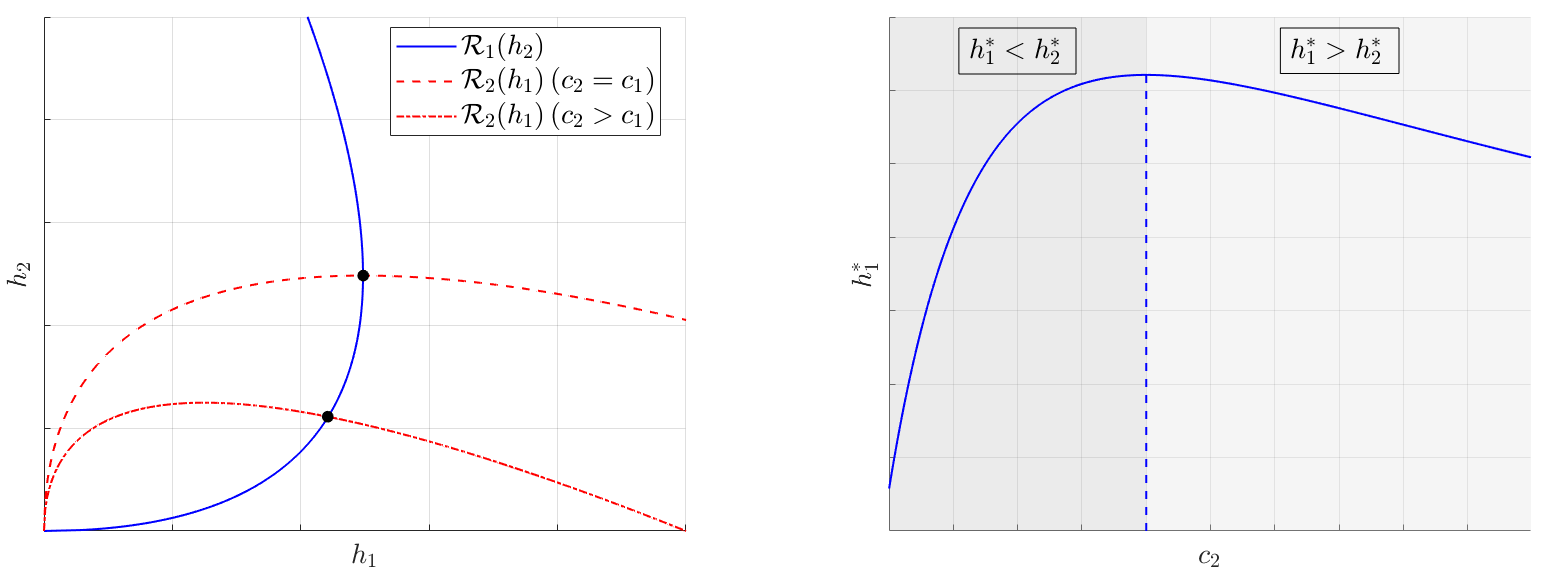
Figure 1: Conceptual visualization of equilibrium hash rates in a system consisting of $N=2$ miners. Left panel: Response functions. Solid blue curve is the response function of miner $1$ with cost $c_{1}>0$. Red curves are the response functions of miner $2$ for the symmetric case $c_{2}=c_{1}$ (dashed line), and for the case $c_{2}>c_{1}$ (dash-dotted line). The equilibrium hash rates, characterized in Proposition 4.1, are determined by the point of intersection of the two curves. Right panel: Equilibrium hash rate $h_{1}^{*}$ of miner $1$ as a function of the cost $c_{2}$ of miner $2$. The dashed line corresponds to the hash rate exerted at the point $c_{2}=c_{1}$, in which case $h_{1}^{*}=h_{2}^{*}$. The hash rate $h_{1}^{*}$ is decreasing in $c_{2}$ to the right of this point, but increasing in $c_{2}$ to the left of this point.

The last part of Proposition 4.6 shows how a change in the cost-per-hash of a given miner imposes an externality on the hash rate shares of its competitors. In this case, the sign of the indirect sensitivity $\widetilde{\Delta}_{i,2}$ is always positive: if the cost of miner $j$ increases, the hash rate share of miner $i$ get larger, even if its hash rate goes down. In other words, if the cost-per-hash of miner $j$ increases, the share of the mining reward earned by all other miners increase at the expense of miner $j$.

These findings have implications for mining centralization. First, we already know that a higher homogeneity among miners results in more of them being active in equilibrium, and thus increases mining decentralization (see Prop. 4.4). Proposition 4.6 additionally shows that increased homogeneity contributes to decentralization, once the set of active miners is fixed. For example, if miner $i$ has a relatively low mining cost, and thus a relatively large hash rate share, then an increase in its cost transfers hash rate share from miner $i$ to other miners. Similarly, if miner $i$ has a relatively high mining cost, and thus a relatively small hash rate share, then this miner would gain hash rate share from other miners if its cost were to decrease.

4.3.3 Sensitivity of Individual Hash Rates to Mining Reward and Mining Capacity

In the previous section, we have argued that a miner’s hash rate depends both directly and indirectly on mining costs. The same holds true for the dependence of hash rates on mining reward and mining capacity, where an indirect dependence again arises through the aggregate hash rate. These dependences are formulated in the following proposition; explicit expressions for all components are provided in equations (B.11) and (B.34) of Appendix B.

Proposition 4.8.

The sensitivities of an active miner’s hash rate $h_{i}^{*}$ to $\gamma$ and $R$ admit the following decompositions,

$$\frac{\partial h_{i}^{*}}{\partial\gamma} =\Delta_{i,1}^{(\gamma)}+\Delta_{i,2}^{(\gamma)},\mkern-36.0mu\mkern-36.0mu \Delta_{i,1}^{(\gamma)} <0,\mkern-36.0mu\mkern-36.0mu \Delta_{i,2}^{(\gamma)}>0\;\; \Longleftrightarrow\;\;\frac{h_{i}^{*}}{H^{*}}<\frac{1}{2},$$ (4.16)

$$\frac{\partial h_{i}^{*}}{\partial R} =\Delta_{i,1}^{(R)}+\Delta_{i,2}^{(R)}>0,\mkern-36.0mu\mkern-36.0mu \Delta_{i,1}^{(R)} >0,\mkern-36.0mu\mkern-36.0mu \Delta_{i,2}^{(R)}<0\;\; \Longleftrightarrow\;\;\frac{h_{i}^{*}}{H^{*}}<\frac{1}{2}.$$ (4.17)

Furthermore, the derivatives of $h_{i}^{*}/H^{*}$ with respect to $\gamma$ and $R$ are increasing in $i$, for $1\leq i\leq n$.

The impact of $\gamma$ on a miner’s hash rate depends on the miner’s size. First, the direct sensitivity $\Delta_{i,1}^{(\gamma)}$ is negative for all miners, because a higher value of $\gamma$ increases the marginal cost of hashing. However, the explicit expression provided in Equation (B.11) for $\Delta_{i,1}^{(\gamma)}$ and $\Delta_{i,2}^{(\gamma)}$ shows that for small enough miners, the indirect sensitivity is positive and large enough to outweigh the direct sensitivity. Intuitively, this is because miners who exert large hash rates, and are thus capacity constrained, are forced to reduce their hash rates. This, in turn, increases the marginal gain of mining, and allows smaller miners who are not capacity constrained to expand. Observe from Table 1 that the net effect of an increase in $\gamma$ on the aggregate hash rate is negative. That is, increased hashing of smaller miners does not fully compensate for the reduction in hash rates by larger miners.

From the above analysis it follows that a tighter capacity constraint (i.e., higher $\gamma$) increases decentralization - smaller miners gain hash rate share at the expense of larger miners. The proposition shows that a larger mining reward has the same effect, even though the hash rate of each miner increases. This can again be understood in terms of the capacity constraint. Specifically, a larger mining reward increases the marginal gain of hashing, leading to larger hash rates, but smaller miners are able to raise their hash rates more than larger miners. Hence, a reduced mining capacity and an increased mining reward not only improves decentralization by increasing the number of active miners (as shown in Section 4.2), but also creates a second decentralization effect by reducing the hash rate of large miners and increasing the hash rate of small miners. This second decentralization effect is material, considering that a fair amount of time and planning is needed to establish new mining operations, so the total number of active miners stays unchanged over short periods of time (see also the discussion in Section 7.1).

5 Miners’ Hardware Investment

In this section, we study the investment in hardware made by miners before participating in the mining competition. We characterize the equilibrium investment profile in Section 5.1. We study how investment affects the mining equilibrium in Section 5.2.

5.1 Equilibrium Investment Profile

We begin by showing the existence of an equilibrium investment $\beta^{*}$, i.e, such that $(\beta^{*},h^{*}(\beta^{*}))$ satisfies equations (3.7)-(3.8), where $h^{*}(\beta^{*})$ is the unique equilibrium hash rate profile corresponding to investment $\beta^{*}$, characterized in Proposition 4.1.

Proposition 5.1.

There exists a unique equilibrium investment $\beta^{*}$ given by

$$\beta_{i}^{*}=\left\{\begin{array}[]{ll}\min\big{\{}\frac{1}{\eta},1\big{\}},&\;1\leq i\leq n,\\ 0,&\;n<i\leq N,\end{array}\right.$$ (5.3)

for some $2\leq n\leq N$. The equilibrium set of active miners defined in Eq. (3.3) is such that $A(0)\subseteq A(\beta_{i}^{*})$. Furthermore, the number $n$ of active miners is decreasing in the fixed cost $K$ incurred by miners.

Observe that the equilibrium number $n$ of active miners depends on the investment profile $\beta^{*}$, and is thus an endogenous quantity. However, this number can be characterized in terms of model primitives as the largest $i\geq|A(0)|$ such that miner $i$ is active in the mining equilibrium corresponding to the investment profile $\beta^{(i)}$ given by $\beta_{j}^{(i)}=\min\{1/\eta,1\}$ for $1\leq j\leq i$, and $\beta_{j}^{(i)}=0$ for $i<j\leq N$.

With investment, the number of active miners either increases or stays the same as without investment. Because of gains in efficiency, miners who already were active without investment remain active after investment, although their shares of the aggregate hash rate may change. Inactive miners, instead, may not be able to benefit sufficiently from investment to enter the mining competition, either because of too high initial costs, or because of the fixed cost incurred by entry (see Eq. (3.6)).

An active miner $i$ chooses a level of investment $\beta_{i}^{*}$ which minimizes its cost-per-hash $c_{i}(\beta_{i})$. This follows from the fact that the profit of miner $i$ is decreasing in its cost of mining (see Prop. B.1). As a result, the investment of miner $j\neq i$ does not impose an externality on the investment of miner $i$.

The absence of these investment externalities is consistent with existing practices, where each miner aims to maximize its own efficiency to remain competitive. Namely, while the overall system hash rate is readily observed, each miner does not observe the hash rates and mining costs of its competitors, or even the number of active miners. This is reflected in the objective function of miner $i$, where the only quantity that depends on the actions of other miners is the aggregate hash rate.

It follows directly from equation (3.1) that the reduction in cost-per-hash of an active miner $i$ because of investment is

$$I_{i}:=c_{i}(0)-c_{i}(\beta_{i}^{*})=\left\{\begin{array}[]{ll}\frac{1}{2\eta}(\tilde{c}_{i}-\tilde{c}_{0}),&\;\eta>1,\\ \big{(}1-\frac{\eta}{2}\big{)}(\tilde{c}_{i}-\tilde{c}_{0}),&\;\eta\leq 1.\end{array}\right.$$ (5.6)

The above formula highlights how initial mining efficiencies and adjustment costs impact the efficiency gains from investment. First, the cost reduction is greater if the miner is less efficient to begin with. Second, the cost reduction is decreasing in the adjustment cost parameter $\eta$, which reflects frictions faced by miners when it comes to investing in new hardware. Overall, the intuition is that for miners with a low initial cost, the cost reduction from investing in new hardware is limited, as they are already highly efficient. Hence, investment reduces the technological gap between miners.

5.2 Investment and Mining Equilibrium

In this section, we study how the mining equilibrium changes with low levels of investment. Miners make small investments if the adjustment cost is sufficiently convex, i.e., if $\eta$ is large. Specifically, it can be seen from (5.3) that $\beta^{*}$ is decreasing in $\eta$. It follows that if $\eta$ is sufficiently large, the set of active miners remains the same after investment, i.e., $A(\beta^{*})=A(0)$.

We use $\bar{I}:=\sum_{i=1}^{n}I_{i}$ to denote the aggregate cost reduction for all active miners, where $I_{i}$ is given by (5.6), and we denote by $I_{-i}:=\bar{I}-I_{i}$ the cost reduction of all miners except $i$. We also recall that $c^{(n)}(0)$ is the cumulative cost-per-hash of all active miners without any investment.

The following propositions provide approximate formulas for how hash rate levels, hash rate shares, and profits change with investment. The accuracy of these approximations is theoretically guaranteed when the adjustment costs are large. In Appendix A, we verify numerically that they remain accurate for small adjustment costs.

Proposition 5.2.

The aggregate hash rate in equilibrium, with and without investment, satisfies

$$H^{*}(\beta^{*}) =H^{*}(0)+aH^{*}(0)\bar{I}+O(\bar{I}^{2}).$$ (5.7)

The coefficient $a>0$ admits an explicit expression given in (B.82). Furthermore, $a$ is increasing in $c^{(n)}(0)$, and decreasing in $\gamma$.

The proposition shows that the investment of each miner increases the aggregate hash rate, and that the relative increase $H^{*}(\beta^{*})/H^{*}(0)$ is larger if miners are collectively less efficient to begin with, i.e., if $c^{(n)}(0)$ is large. The reason is that the reduction in mining costs is increasing in the miners’ initial costs; thus, investment has a stronger impact if the initial costs are large. Moreover, investment has a greater impact on the aggregate hash rate if $\gamma$ is small, because less capacity constrained miners are able to increase their hash rates more.

Proposition 5.3.

The relation between the hash rate of miner $i$, with and without investment, is as follows,

$$h_{i}^{*}(\beta^{*}) =h_{i}^{*}(0)+a_{i}I_{i}+a_{-i}\bar{I}_{-i}+O(\bar{I}^{2}),$$ (5.8)

where the coefficients $a_{i}$ and $a_{-i}$ are given explicitly in (B.99), and satisfy

$$a_{i}>0,\qquad a_{-i}<0\;\;\Longleftrightarrow\;\;\frac{h_{i}^{*}(0)}{H^{*}(0)}<\frac{1}{2}.$$ (5.9)

The equilibrium hash rate share of an active miner $i$, with and without investment, satisfies

$$\frac{h_{i}^{*}(\beta^{*})}{H^{*}(\beta^{*})} =\frac{h_{i}^{*}(0)}{H^{*}(0)}+\alpha_{0}\big{(}(1-\alpha_{i})I_{i}-\alpha_{i}\bar{I}_{-i}\big{)}+O(\bar{I}^{2}),$$ (5.10)

where the coefficients $\alpha_{0}>0$ and $\alpha_{i}\in(0,1)$ are given explicitly in (B.89). Furthermore, $(1-\alpha_{i})I_{i}-\alpha_{i}$ is increasing in the initial cost $\tilde{c}_{i}$ of miner $i$.

The investment of miner $i$ leads to an increase of its own hash rate. However, there is an externality equal to $a_{-i}\bar{I}_{-i}$ imposed by the investment of other miners on the hash rate of miner $i$ (see Section 4.3.2 for a discussion of the condition on $h_{i}^{*}(0)/H^{*}(0)$). Since other miners also invest to become more competitive, miner $i$ is unable to capture the full benefit of his investment.

In accordance with intuition, the hash rate share of each miner does not change with investment if miners are initially equally efficient. However, this is no longer the case if there is heterogeneity in the miners’ initial costs. It then follows from the proposition that the change in hash rate share is larger for miners with higher initial costs. Hence, investment leads to greater decentralization, i.e., the hash rate share of smaller miners increases while that of larger miners decrease. The mining capacity constraint plays a key role in producing this effect. Because smaller miners are less capacity constrained to begin with, the efficiency gains from their investment allows them to overcome the negative externalities imposed by the investment of other miners. As the capacity constraint becomes less binding, i.e., as $\gamma$ gets smaller, this advantage is reduced and minimized in the limiting case of $\gamma=0$, i.e., when all miners have unbounded capacity.

Next, we analyze the impact of investment on mining profits. We denote by $\pi_{i}^{*}(\beta)$ the profit of miner $i$ in the mining equilibrium corresponding to the investment profile $\beta$.

Proposition 5.4.

The relation between the profit of miner $i$, with and without investment, is as follows,

$${\pi^{*}_{i}(\beta^{*})} =\pi^{*}_{i}(0)+h_{i}^{*}(0)\big{(}b_{i}I_{i}+b_{-i}\bar{I}_{-i}\big{)}+O(\bar{I}^{2}),$$ (5.11)

where the coefficients $b_{i}>0$ and $b_{-i}<0$ are given explicitly in (B.115). Furthermore, $b_{i}I_{i}+b_{-i}\bar{I}_{-i}$ is increasing in the initial cost $\tilde{c}_{i}$ of miner $i$, and negative for small enough values of $\tilde{c}_{i}$.

Investment impacts the profit of a miner similarly to how it affects its hash rates. In Proposition 5.3, we argue that smaller miners are able to gain hash rate share at the expense of larger miners. Proposition 5.4 additionally states that smaller miners are those who increase their profits the most, while the profits of larger miners can even decrease. These theoretical findings are supported by the global cryptocurrency studies discussed in Remark 3.1, where it is reported that the primary concern of large miners is earning lower profits due to increased competition.

Next, we study welfare in the mining ecosystem, defined as the sum of all miners’ profits. We denote by $\Pi^{*}(\beta):=\sum_{i=1}^{n}\pi_{i}^{*}(\beta)$ the aggregate profit in the mining equilibrium corresponding to the investment profile $\beta$. As we show in the next proposition, welfare increases with investment in a homogeneous system.

Proposition 5.5.

If miners are homogeneous in their costs, then the relation between the aggregate profit of all miners, with and without investment, is as follows,

$$\Pi^{*}(\beta^{*})=\Pi^{*}(0)+bH^{*}(0)\bar{I}+O(\bar{I}^{2}),$$ (5.12)

where the coefficient $b>0$ is given explicitly in (B.125). Furthermore, $b$ converges to zero as $\gamma\to 0$.

The above proposition implies that more efficient mining allows capacity constrained miners to reap the benefit of their investment. However, as mining capacity grows unbounded, i.e., as $\gamma\to 0$, the profit becomes independent of investment. That is, with unbounded capacity, the benefits of a higher mining efficiency are exactly offset by the costs of a higher aggregate hash rate.

If miners are heterogeneous in their initial hashing costs, the aggregate profit may either increase or decrease with investment. If there is little heterogeneity, then the profit increases, as in the fully homogeneous case discussed above. However, if there is significant heterogeneity, the profit may decrease. The intuition is that while smaller miners are able to increase their profits, the scale of their operations is smaller. Hence, the increase in their profits does not fully compensate for the profit reduction of larger miners - such miners do not benefit as much from investment, either because they are already very efficient in their mining, or because they are too capacity constrained. Formally, this can be seen from the profit formula (5.11), where small and negative values of the term $b_{i}I_{i}+b_{-i}\bar{I}_{-i}$ are associated with smaller values of $\tilde{c}_{i}$, and thus multiplied by larger values of $h_{i}^{*}(0)$.

6 Mining Centralization and Network Security

In this section, we construct measures of mining centralization and network security. We then evaluate these measures at the mining equilibrium, and discuss how they depend on investment, mining reward, and mining capacity.

We begin by estimating the model parameters based on statistics from the Bitcoin network and using the model’s equilibrium solution.

(i) Mining reward:

We set $R=\$20\times 10^{6}$, which is the average daily Bitcoin mining reward in the period from January 1st, 2020, to April 30th, 2021 (see Fig. 4).

(ii) System hash rate:

We estimate $H$ by taking the average Bitcoin network hash rate in the period from January 1st, 2020, to April 30th, 2021. This yields $H=120$ million TH/s (see Fig. 4).

(iii) Number of miners:

We base our estimate on the Global Cryptocurrency Benchmarking Study (Hileman and Rauchs (2017)), where 11 of the participants are designated as large mining organizations, and estimated to cover over 50% of the total professional mining sector in terms of hash rate. Hence, we approximate the number of miners to $N=20$.

(iv) Mining costs:

We measure the cost-per-hash of a single miner as the cost of generating one million TH/s for one day (24 hours). We base our estimates on the power consumption of AntMiner S19 Pro, which is Bitmain’s latest model, released in May 2020. As of April 2021, it is the most energy efficient commercially available mining hardware, together with MicroBT’s WhatsMiner M30S$++$. AntMiner S19 Pro has an energy efficiency of 29.5 J/TH, and we assume an electricity cost of $0.05 per kWh. The latter is a standard estimate of the average electricity cost incurred by large miners. Altogether, this yields a cost of $0.0295\times 0.05\times 24=\$0.0355$ per TH/s for one day. We set the cost of the most efficient miner to this value, i.e., $c_{1}=0.0355$.

Recall from Section 4.2 that miner $i$ exerts a positive hash rate in equilibrium if its cost $c_{i}$ is lower than the break-even cost $R/H^{*}$. We set the mining costs $(c_{i})_{1\leq i\leq N}$ as $N$ evenly spaced points between $c_{1}$, as estimated above, and $R/H$, where $H$ is estimated as in (ii).

(v) Capacity constraint:

We invert the formula for the equilibrium hash rate $H^{*}$, given in equation (4.7), and imply the parameter value

$$\gamma=\frac{1}{H^{*}}\Big{(}\frac{(n-1)R}{H^{*}}-c^{(n)}\Big{)}.$$ (6.1)

We set $H^{*}$ to the value estimated in (ii). If all miners are active, i.e., $n=N=20$, then $\gamma=0.0095\times 10^{6}$.

(vi) Adjustment costs:

Recall that the adjustment costs are of the form (3.2), and $\eta\geq 0$ governs how much miners are able to increase their efficiency. It follows from formula (5.6) that

$$c_{i}(\beta^{*}_{i})=\tilde{c}_{i}-\frac{\tilde{c}_{i}-\tilde{c}_{0}}{2}\quad\Longleftrightarrow\quad\eta=1.$$ (6.2)

That is, less than half (more than half) of the efficiency gap $\tilde{c}_{i}-\tilde{c}_{0}$ is bridged by investment if $\eta>1$ ($\eta<1$). A reasonable lower bound for the value of $\eta$ is therefore given by $\eta=1$, as in that case $\beta_{i}^{*}=1$ and miner $i$ upgrades its entire stock of hardware.

We next develop and analyze the measure of mining centralization and network security. For Bitcoin and other proof-of-work cryptocurrencies, the security of the network depends on the distribution of hashrate among miners, i.e., the level of decentralization. To quantify the implications of investment on mining centralization, we defining the following function,

$$F(k):=\left\{\begin{array}[]{ll}0,&\;k=0,\\ \sum_{i=1}^{k}\frac{h_{i}^{*}}{H^{*}},&\;k=1,2\ldots,n,\\ 1,&\;k=n.\end{array}\right.$$ (6.6)

It follows directly from the definition that $F(k)$ is the total hash rate share of the $k$ largest miners. The domain of the function $F$ can be extended to non-integer values via linear interpolation. The resulting function is increasing and concave, and degenerates to a straight line if and only if miners are homogeneous and thus all exert the same hash rate. The steeper the function $F$ is for small values of $k$, the greater the extent of mining centralization.

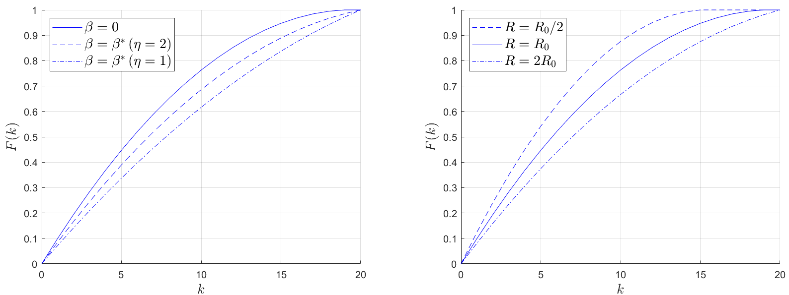
Figure 2: Plot of the hash rate function in (6.6). Left panel: Effect of investment on mining centralization. The solid line correspond to the mining equilibrium without investment ($\beta=0$), and the dashed and dash-dotted lines correspond to mining equilibria with investment ($\beta=\beta^{*}$). We set the model parameters as described in Section 6. Right panel: Effect of mining reward on mining centralization. The model parameters are chosen as described in Section 6, with $R_{0}=20\times 10^{6}$ as in part (i) therein.

It is evident from the left panel of Figure 2 that $F$ is closer to a straight line if the equilibrium hash rates account for investment, and more so if adjustment costs are smaller. This confirms the implications of our model highlighted in Section 5.2, i.e., that investment steers the mining system towards decentralization - a larger number of miners controls any given fraction of the overall hash rate.

The right panel of Figure 2 shows that a higher mining reward also leads to greater decentralization, consistent with our analysis in Section 4.3.3. This implies that if the market capitalization of a coin increases, mining would not become increasingly centralized, i.e., exhibit “the rich getting richer” phenomenon. The rationale offered by our model is that existing mining facilities are not able to increase their hash rate indefinitely, which allows smaller miners to grow and new miners to enter. This is consistent with the fact that Bitcoin mining seems to be less concentrated, both geographically and in terms of hash rate ownership, than commonly indicated by public discourse (see Rauchs et al. (2018)).

Remark 6.1.

As the Bitcoin network has grown larger, the cost of getting anywhere close to the 51% attack threshold has become out of reach for most entities. In addition to the network consuming as much electricity as a small country, the sheer amount of mining hardware required, which is in short supply, is all but impossible to obtain. This is consistent with our model, where a miner with zero cost-per-hash still does not manage to dominate the mining competition, because of limited capacity.

In practice, a small number of large mining pools commonly accounts for over 50% of the Bitcoin network hash rate, but this is unlikely to lead to an attack. Even if a mining pool operator with malicious intent were to successfully implement a 51% attack, such an event would be discovered quickly, and be self-destructive for the mining pool because miners, whose business model is tied to the success of Bitcoin, would quickly switch to other mining pools. In fact, the mining pool Ghash.io came close to the 51% threshold in 2014, seemingly with no intent to attack, but this still prompted miners to voice their concerns and leave the mining pool. ∎

The security of proof-of-work cryptocurrencies relies not only on the network hash rate being distributed among multiple miners, but also on how expensive it is to gain control of a large hash rate share. In fact, the main benefit of a high network hash rate is that it makes the network more secure from attacks. We have seen that technological advancements and investment lead to a higher network hash rate (see Table 1). However, more efficient hardware also leads to lower cost of hashing. To study the net effect of investment on the cost of attacks, observe that $C_{k}:=\sum_{i=1}^{k}(c_{i}h_{i}^{*}+\frac{\gamma}{2}(h_{i}^{*})^{2})$ is the cost of capturing a fraction $p_{k}:=\sum_{i=1}^{k}h^{*}_{i}/{H^{*}}$ of the network hash rate. We then define the cost-of-attack function $TC:[0,1]\mapsto[0,\infty)$ by

$${TC(p_{k})=C_{k},\quad 1\leq k\leq n,}$$ (6.7)

and by linear interpolation for $p\notin\{p_{k},\;1\leq k\leq n\}$. The left panel of Figure 3 shows that investment has a small impact on this function. However, the right panel shows that the value of the mining reward has a significant impact. Intuitively, this is because a higher mining reward leads to a higher hash rate, just like investment does, but the cost of mining stays the same, resulting in larger values of the function $TC$.

Since a smaller mining reward goes hand in hand with a smaller hash rate, this supports the common belief that coins with low hash rates are susceptible to cheap 51% attacks - only a small number of miners from larger coins need to switch to a smaller coin in order to control 51% of the smaller coin’s network hash rate (see also Remark 6.2). In particular, this means that emerging coins with low market capitalization are less secure. It is also worth noting that concentration of hash rate below the 51% barrier also presents danger to the network, for example due to selfish mining attacks (see, e.g., Eyal and Sirer (2014)).

The effect of mining reward on the cost of attacks also has implications for more mature cryptocurrencies like Bitcoin. To see that, first note that transaction fees and block rewards represent the security spending of the network, which is paid for by users of the network, through transaction fees, and by holders of coins, through inflationary block rewards. In principle, the security spending of the network should be large enough in absolute terms to deter attacks, i.e., make them expensive, but also large enough as a percentage of the market capitalization because the damage of a successful attack varies with the market value of Bitcoin. In coming years, Bitcoin will continue its gradual shift from paying miners primarily through block reward to paying miners primarily through transaction fees. With diminishing block rewards, Bitcoin therefore needs to develop a persistent fee market structure to sustain the mining reward and maintain security (see Figure 5). Whether that will happen largely depends on the eventual level of Bitcoin adoption. If fees are not sufficient to sustain the mining reward, our results indicate that the network becomes vulnerable to attacks. This rhymes with one of Nakamoto’s original propositions regarding the future of Bitcoin: “When the reward gets too small, the transaction fee will become the main compensation for nodes. I’m sure that in 20 years there will either be very large transaction volume or no volume”. An alternative view is that security spending should be proportional to transactional volume, i.e., a flow variable rather than a stock variable (Budish (2018)). This is based on the notion that 51% attacks can only endanger the last few blocks appended to the blockchain, so the reward from such an attack is proportional to the value of recent transactions. In this case, the same principle applies, i.e., that transaction fees have to grow to sustain the mining reward, as the network transitions to a fee-based reward system.

Remark 6.2.

The function $TC$ in (6.7) gives the cost, for existing miners, of generating a given share of the network hash rate. In addition to this cost, rational self-interest can be considered a backup defense for attacks. Miners invest large amounts of capital into mining facilities whose profitability is tied to the success of the network. Hence, even if miners were to achieve a successful attack, it would likely damage the market capitalization of the network, and thus their own income and net worth.

However, attacks from entities outside of the network have become of increased concern with the emergence of cloud mining services that offer customers the possibility to participate in mining without having to own hardware themselves. That is, the attacker is not exposed to the opportunity cost of future revenue generated by the hardware. For many smaller coins, there is hash rate available to rent that is orders of magnitude larger than their network hash rates. As part of the Digital Currency Initiative, launched by the MIT Media Lab, a system was constructed to actively monitor proof-of-work cryptocurrencies with the goal of detecting 51% attacks. Since launching the system in June 2019, over 40 successful attacks have been detected, with evidence that hash rate rental markets have been used to perform some of them. ∎

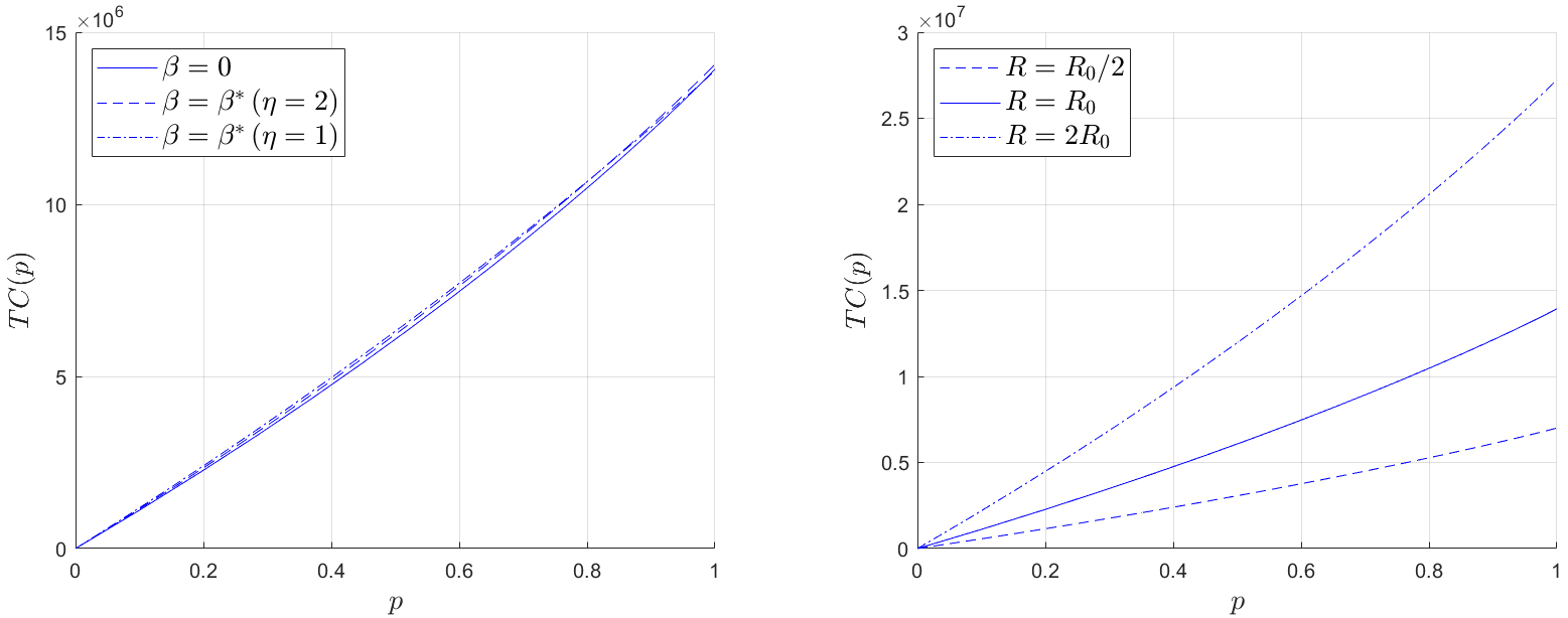
Figure 3: Plot of the total cost function in (6.7). Left panel: Effect of investment on the cost of attacks. Right panel: Effect of mining reward on the cost of attacks. The model parameters are chosen as in Figure 2.

7 Empirical Analysis

In this section, we provide empirical support for the most significant equilibrium implications of our model. In Section 7.1, we present empirical patterns of the Bitcoin mining network. In Section 7.2, we provide statistical evidence for the predicted relationship between mining reward and the aggregate hash rate. All data used in this section is obtained from https://www.blockchain.com/.

7.1 Empirical Patterns of Cryptocurrency Mining

The mining reward, i.e., the revenue from mining, consists of coinbase block rewards plus transaction fees paid to miners. These fees are voluntarily attached by users to increase the probability that their transactions are included in mined blocks appended to the ledger. It is evident from Figure 4 that transaction fees are a small component of the mining reward, and that there is a strong positive co-movement between the mining reward and the price of Bitcoin. We also observe a positive relation between the value of transaction fees and the price of Bitcoin. Intuitively, a higher price is the result of increasing demand for Bitcoin, which in turn implies a larger number of transactions. Hence, higher fees are required to incentivize miners to include a given transaction in a block.

The evidence provided above indicates that transaction fees have so far had a limited impact on the incentives of miners, and that both coinbase block rewards and fees are primarily driven by a common factor - the price of Bitcoin. A notable exception is the dramatic increase in transaction fees observed in December 2017. The subsequent decline in fees is largely attributed to increased adoption of the so-called SegWit update to the Bitcoin protocol, which effectively acted as a block-size increase and thus allowed more transactions to be processed per block. While Bitcoin has been in existence for over a decade, and around 90% of its 21 million coins have already been mined, transaction fees still constitute a small component of mining revenues. As pointed out in Easley et al. (2019), the growing market capitalization of a coin can delay the point where transaction fees take over, and this has been the case for Bitcoin.

Figure 5 shows that as Bitcoin’s market capitalization has grown, the security spending (see Section 6) has grown as well, but the percentage of the market capitalization spent on security has declined. Observe that there is a noticeable drop in this percentage around the Bitcoin halving events in November 2012, July 2016, and May 2020, when the reward for mining a block was halved. Figure 5 shows that security spending was large in the early days relative to market capitalization, which is expected for emerging coins. Since then it has tapered off and was largely constant between the 2016 and 2020 halving events.

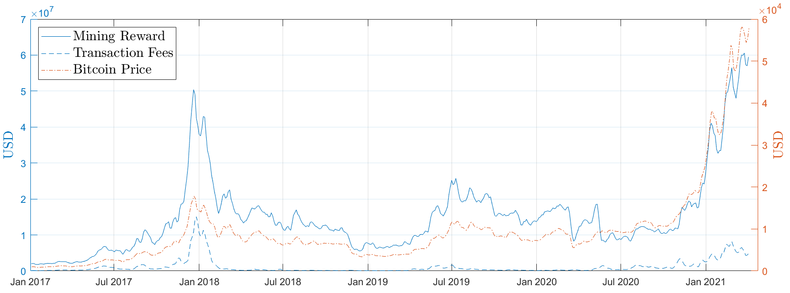
Figure 4: Left y-axis: the total reward earned by miners (coinbase block rewards and transaction fees), and the component of total reward due to transaction fees. Right y-axis: price of Bitcoin. The plot shows seven-day averages, computed every three days between January 2017 and April 2021.

Figure 6 shows that there exists an overall positive relationship between the system hash rate and the Bitcoin price, but with a few notable discrepancies. For example, in the first half of 2018, there was a significant drop in the price of Bitcoin, but the hash rate kept climbing until finally dipping at the end of that year. Importantly, this period was preceded by an unprecedented Bitcoin boom. Such periods of Bitcoin mania are likely to trigger significant investments in mining facilities, which then become operational with a time lag. In this specific case, the effect was to raise the system hash rate during the market drop in 2018. The same pattern is observed in the second half of 2019, where the Bitcoin price trended downwards while the hash rate kept climbing. Again, this occurred following a rally in the first half of 2019, leading to investments that contributed to increasing the hash rate during a time when the Bitcoin price was dropping. The third, and perhaps best representation of the above pattern, is the extreme surge in the price of Bitcoin during the second half of 2020, which has not yet been associated with an equally large increase in the system hash rate. This can be explained by the inability of miners to expand their operations immediately, and suggests that the hash rate may keep rising in the second half of 2021, even if the price of Bitcoin starts falling. The above argument is supported by the 2nd Global Cryptoasset Benchmarking Study (Rauchs et al. (2018)). Based on proprietary data covering six major proof-of-work cryptocurrencies, including Bitcoin and Ethereum, it is reported that “hashers often cannot immediately increase production when running at full capacity”, resulting in hash rate growth lagging behind market price growth.

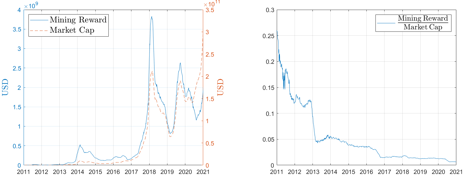
Figure 5: Left panel: Solid line plots total mining reward earned by miners, computed as the annualized sum of mining reward over a running three-month window. Dashed line shows the Bitcoin market capitalization, computed as the average market capitalization over a running three-month window. Right panel: Mining reward as a proportion of Bitcoin market capitalization, with both quantities computed as in the left panel.

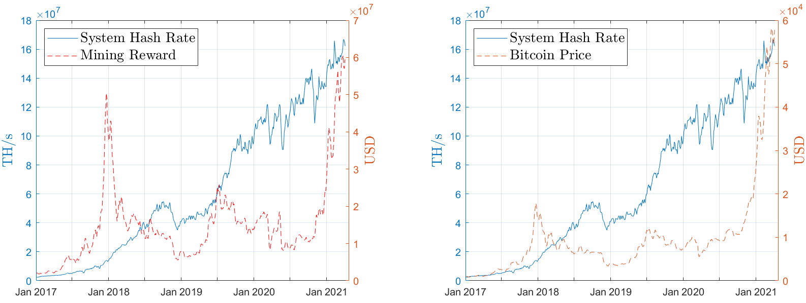
Figure 6: Left panel: System hash rate (left y-axis) and total reward earned by miners per day (right y-axis). Right panel: System hash rate (left y-axis) and price of Bitcoin (right y-axis). The plots show seven-day averages, computed every three days between January 2017 and April 2021.

7.2 Hash Rate vs. Mining Reward: Statistical Evidence

In Proposition 4.1, we have shown that if $\gamma>0$, the equilibrium hash rate $H^{*}$ increases like the square root of the mining reward $R$ (see also discussion in Section 4.3.1). It follows that

$$1+r_{H^{*}}(t)\approx\sqrt{1+r_{R}(t)},$$ (7.1)

where $r_{H^{*}}(t)$ and $r_{R}(t)$ are equilibrium hash rate and mining reward returns between times $t-1$ and $t$. More generally, if $H^{*}$ increases like a power $\beta$ of $R$, we have

$$1+r_{H^{*}}(t)\approx(1+r_{R}(t))^{\beta}.$$ (7.2)

To statistically test this relationship, we consider the linear regression model

$$\log\big{(}1+r_{H}(t)\big{)}=\alpha+\beta\log\big{(}1+r_{R}(t-1)\big{)}+\epsilon(t),$$ (7.3)

where $\epsilon$ is a vector of idiosyncratic errors and $r_{H}(t)$ and $r_{R}(t)$ are, respectively, historical three-month hash rate and mining reward returns. We compute these returns using monthly averages of hash rates and mining rewards. For example, if $t$ is equal to July 15, then $r_{H}(t)$ is the simple return between the average hash rate in April and the average hash rate in July, and $r_{R}(t-1)$ is the simple return between the average mining reward in January and the average mining reward in April. We use lagged values for mining reward, because hash rates typically respond with a lag to changes in the mining reward, as documented in Section 7.1.

It is evident from Figure 7 that there exists a sublinear relationship between $r_{H}(t)$ and $r_{R}(t-1)$. This pattern is statistically confirmed by our regression analysis, which yields the estimate $\hat{\beta}=0.34$ (see Table 2). These findings are consistent with the equilibrium hash rates when $\gamma>0$, given in Proposition 4.1, and also reflect economic intuition. That is, we expect capacity constraints to prevent miners from increasing their hash rates proportionally to increases in the mining reward, as the marginal cost of mining becomes higher as the exerted hash rate increases.

Remark 7.1.

The objective function (3.6) can be generalized to

$$\pi_{i}=\frac{R}{H}h_{i}-c_{i}h_{i}-\frac{\gamma}{1+\delta}h_{i}^{1+\delta},$$ (7.4)

where $\delta>0$, and the expression in (3.6) is then recovered if $\delta=1$. For $\delta\neq 1$, the aggregate hash rate $H^{*}$ does not admit a closed-form representation. However, we can mimic the steps in the proof of Proposition 4.1, and show that if miner heterogeneity is low, then $H^{*}$ behaves approximately like a power $1/(1+\delta)$ of the mining reward $R$. Hence, it follows from (7.2)-(7.3) that the regression estimate $\hat{\beta}\approx 1/3$ in Table 2 is consistent with a coefficient $\delta=2$. This corresponds to a convex capacity constraint which is cubic rather than quadratic. Using the objective function (7.4) would produce results qualitatively similar to those obtained with a quadratic objective function (3.6), the key point being that the marginal cost of mining is increasing in both cases. ∎

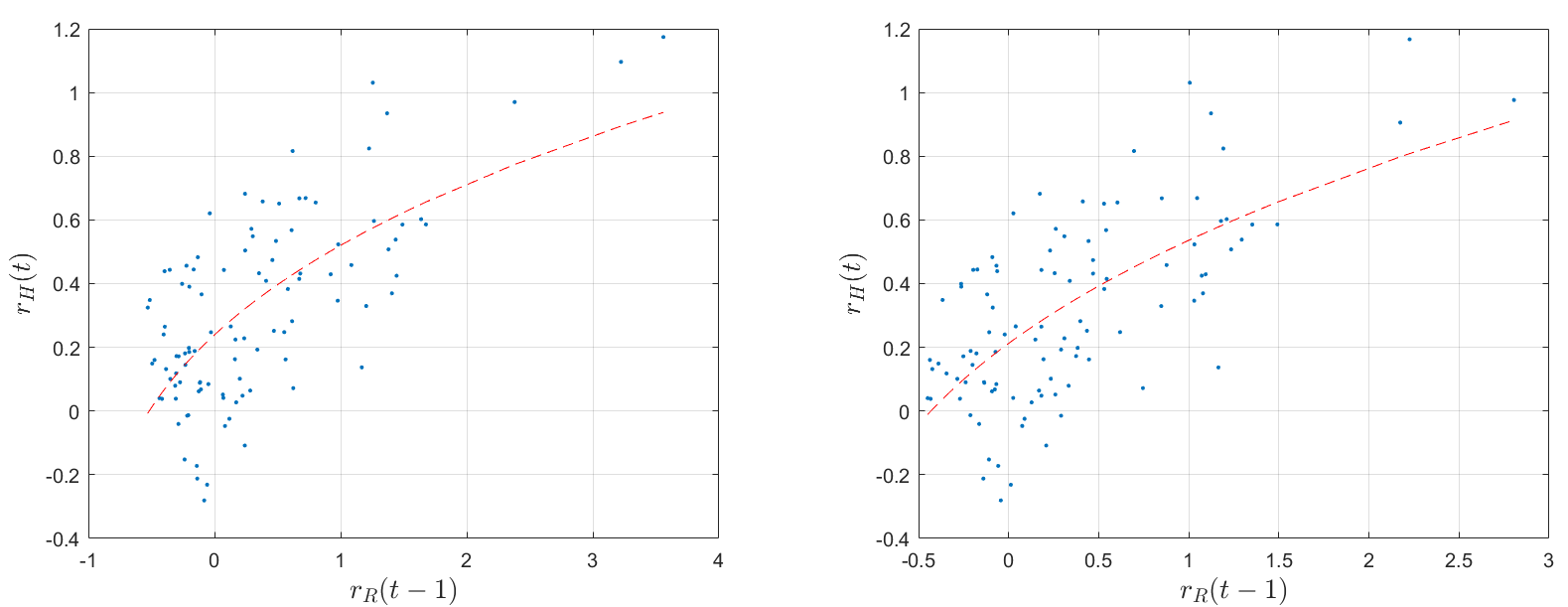
Figure 7: Left panel: Scatter plot of three-month system hash rate returns (y-axis) against lagged three-month mining reward returns (x-axis), computed for biweekly time points between January 2017 and April 2021. The dotted line corresponds to the best fit of the linear model (7.3) - the regression statistics are reported in Table 2. Right panel: Same plot as in the left panel, but with the returns $r_{R}(t-1)$ computed using Bitcoin prices rather than mining rewards. The patterns in both panels are similar, consistently with the fact that the Bitcoin price is a good proxy for the mining reward (see also Fig. 4).

	$\hat{\alpha}$	$\hat{\beta}$	$R^{2}$
$R$	$0.22$	0.29	0.44
$P$	0.19	0.34	0.43

Table 2: Regression estimates for the linear model in Equation (7.3). In the first row of the table ($R$), $r_{R}(t-1)$ is computed using mining rewards. In the second row of the table ($P$), $r_{R}(t-1)$ is computed using Bitcoin prices. The number of observations is $102$, and all parameter estimates are statistically significant with $p$-values smaller than 0.001. Because the Bitcoin price is a good proxy for the mining reward (see Fig.  4), the regression estimates in the two rows of the table are similar.

8 Conclusions

We develop a model of cryptocurrency mining where miners invest in new hardware to improve the efficiency of their operations in a subsequent proof-of-work mining competition. We demonstrate that the nature of the mining competition excludes inefficient miners from participating, in contrast to the original vision of Nakamoto. We argue that mining centralization is lower than indicated by earlier research due to capacity constraints faced by miners. Additionally, we show that the ability of miners to invest in new technology leads to greater decentralization in mining. Hence, while the emergence of specialized mining hardware has resulted in individual miners being replaced by relatively large mining operations, larger miners do not inherently increase their advantage over smaller ones. As advancements in ASIC mining hardware slow down, our model suggests that mining will become a race for access to low-cost electricity.

Our model indicates that investment in new hardware may not have a large impact on the cost of attacking a cryptocurrency network, even though it increases the aggregate hash rate in the network. In contrast, a higher mining reward significantly increases both mining decentralization and network security, which confirms the common wisdom that smaller coins are more vulnerable to attacks. These findings imply that the majority of coins in existence may not be long-lived. They also raise concerns regarding whether transaction fees will be sufficient to sustain mining reward, and thus network security, for maturing cryptocurrencies.

Our study focuses on the behavior of miners and takes other components of the mining value chain as given. We do not directly model the activities of hardware manufacturers, but rather assume the existence of a monopolistic manufacturer that supplies miners with new hardware. From the miners’ point of view, the ASIC hardware industry has been dominated by a single firm, Bitmain, and the hardware of other prominent manufacturers can safely be treated as a substitute good. We also remark that our implicit assumption of a monopolistic manufacturer is consistent with Ferreira et al. (2019), who argue that a single manufacturer will dominate in the blockchain ecosystem.

We also do not consider mining pools in our analysis. Empirical evidence indicates that the size of mining pools is mean-reverting, with honest miners leaving a mining pool that becomes too large (see also Cong et al. (2021)). Additionally, significant constraints have been placed on the ability of pool managers to act in bad faith (see Remark 6.1). When it comes to actual mining, the availability of mining pools is likely to contribute to decentralization. This is because their absence would be more detrimental to smaller miners, who are likely to be worse equipped to face a high variance in their mining revenue, and for which the average time between mined blocks is larger.

Alternatives to the proof-of-work protocol have been proposed, most prominently the proof-of-stake protocol, where miners do not use computational resources to compete for the right to validate transactions, but rather are chosen in proportion to their ownership of the underlying coin. This implies a clear path to centralization in mining: a miner who starts with a larger number of coins has a higher probability of further increase its advantage than a smaller miner has of reducing the initial gap. Our model can be extended to such a proof-of-stake setting where the miners’ initial probabilities of mining a block are determined by their initial coin holdings, and the hardware investment stage is replaced by a stage where miners invest in the underlying coin.

While the size of the Bitcoin network currently dwarfs the size of other networks, there are by now multiple established cryptocurrencies that miners can move their hash rate between. Arguably, for a given level of mining power, only a finite number of networks of significant size can be secured. However, most existing research focuses on a single network, and it remains an open question to understand how allocation of mining power between different networks will impact centralization in individual networks.

In a dynamic extension of our model, we expect the equilibrium hash rate shares of miners to converge over time. A dynamic model would provide a deeper understanding of centralization forces in cryptocurrency mining. For example, the effect of investment is to some extent permanent, and its benefit is path-dependent. Investment thus effectively allows miners to remain competitive over time and protected against a significant drop in the mining reward, which could otherwise force them out of business. Finally, an important factor to consider is how volatility of mining reward affects mining centralization. Cryptocurrencies are a highly volatile asset class, and, as mentioned above, fluctuations in mining revenue may present greater challenges for smaller miners. We leave these questions for future research.

Appendix A Accuracy of Approximation Formulas in Section 5.2

We verify the accuracy of the approximation formulas used to analyze the effect of investment on equilibrium hash rates and mining profits. Figure 8 confirms our analytical findings from Section 5.2, i.e., that smaller miners gain hash rate shares and increase their profits, while the opposite is true for larger miners. It is also evident from the figure that these trends magnified for smaller values of $\eta$, i.e., lower adjustment costs, which leads to larger investment levels.

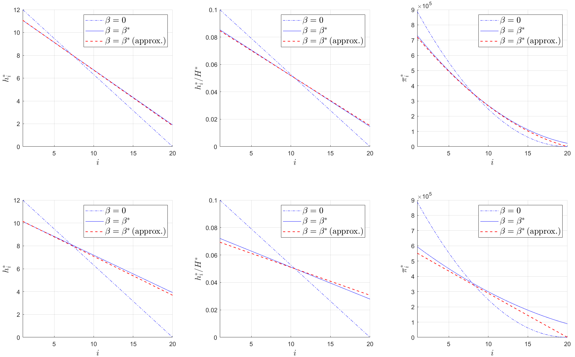
Figure 8: The left and middle panels plot the hash rates and hash rate shares of miners, indexed by $i$, with and without investment (i.e., $\beta=\beta^{*}$ and $\beta=0$). The red dotted lines show the approximations in Proposition 5.3. The right panels plot the profits of miners with and without investment. The red dotted lines plot the approximation in Proposition 5.4. The model parameters are set as described in Section 6, with $\eta=2$ (upper panels) and $\eta=1$ (lower panels).

Noticeably, the approximation formulas for both hash rates and profits, given in Propositions 5.2 and 5.4, closely resemble their exact counterparts. The accuracy of the approximations increases as $\eta$ gets larger, but it remains good for both hash rates and hash rate shares if $\eta$ is small, and within acceptable levels for mining profits. It is worth observing that $\eta=1$ corresponds to a reasonable lower bound for the value of $\eta$ (see Section 6).

Appendix B Proofs of Propositions

Proof of Proposition 4.1:

Sufficient conditions for the existence of a pure-strategy equilibrium are (i) concavity of $\pi_{i}$ in $h_{i}$, (ii) continuity of $\pi_{i}$ in $h_{i}$ and $h_{-i}$, and (iii) the strategy space of miner $i$ being compact and convex. For the concavity of $\pi_{i}$ we have

$$\frac{\partial\pi_{i}}{\partial h_{i}}=\frac{H-h_{i}}{H^{2}}R-c_{i}-\gamma_{i}h_{i},\qquad\frac{\partial^{2}\pi_{i}}{\partial h_{i}^{2}}=-2\frac{H-h_{i}}{H^{3}}R-\gamma_{i}<0.$$ (B.1)

For the continuity properties it is easy to see that for any given $h_{-i}$ (resp., $h_{i}$), the objective function $\pi_{i}$ is continuous in $h_{i}$ (resp., $h_{-i}$). The strategy space of miner $i$ is $[0,\infty)$, which is unbounded. However, since $\pi_{i}<0$ for $h_{i}>R/c_{i}$, the strategy space of miner $i$ can be restricted to the compact and convex set $[0,R/c_{i}]$.

To show uniqueness, first observe that any equilibrium will consist of at least two active miners. Namely, if only a single miner applies a positive hash rate, then a marginal reduction in its hash rate will increase the value of its objective function. Similarly, if no miner applies a positive hash rate, then each miner has an incentive to marginally increase its hash rate. In both cases we have a contradiction. Next, observe that if miner $k+1$ is active in equilibrium, then miner $k$ cannot be inactive, because in that case we would have

$$MG_{k}:=\frac{R}{H}>\frac{R}{H}\Big{(}1-\frac{h_{k+1}}{H}\Big{)}=MG_{k+1}=MC_{k+1}=c_{k+1}+\gamma_{k+1}h_{k+1}>c_{k}=:MC_{k},$$ (B.2)

which is a contradiction. Using these two facts, it is easy to show inductively that in a game consisting of a total of $N_{0}$ miners, where $2\leq N_{0}\leq N$, the equilibrium must be unique. When showing the result for $N_{0}+1$, given that the results holds for $N_{0}$, we must consider two cases. First, if miner $N_{0}$ is not active in the unique equilibrium with a total of $N_{0}$ miners, then the same equilibrium is also unique in a game with a total of $N_{0}+1$ miners. Second, if miner $N_{0}$ is active, then miner $N_{0}+1$ is active if and only if $c_{N_{0}+1}<R/H_{N_{0}}$, where $H_{N_{0}}$ is the overall hash rate in the equilibrium with a total of $N_{0}$ miners. It follows that the equilibrium is unique in a game of $N_{0}+1$ miners.

We now derive the equations for the unique equilibrium hash rates. Summing over the first-order condition (4.8) of active miners gives

$$0=\frac{n-1}{H}R-c^{(n)}-\gamma H=\frac{1}{H}\big{(}(n-1)R-c^{(n)}H-\gamma H^{2}\big{)}.$$ (B.3)

The aggregate equilibrium hash rate $H^{*}$ is then given by (4.7), where the case $\gamma>0$ requires solving a second order polynomial which can be shown to have a unique positive solution. The equation for the hash rate $h_{i}^{*}$ then follows from the first-order condition (4.8) of miner $i$. ∎

Proof of Proposition 4.3:

The profit-per-hash of an active miner $i$ is

$$\frac{\pi_{i}^{*}}{h_{i}^{*}}=\frac{R}{H^{*}}-c_{i}-\frac{\gamma}{2}h_{i}^{*}=\frac{R}{H^{*}}-(c_{i}+\gamma h_{i}^{*})+\frac{\gamma}{2}h_{i}^{*},$$ (B.4)

which is decreasing in $i$ because $c_{i}+\gamma h_{i}^{*}$ is increasing in $i$, by Proposition 4.2, and $h_{i}^{*}$ is decreasing in $i$, by Proposition 4.1. It follows that the profit $\pi_{i}^{*}$ is also decreasing in $i$. ∎

Proof of Proposition 4.4:

From Proposition 4.1 it follows that miner $i$ is active in equilibrium if and only if $R/H^{*}>c_{i}$. Thus,

$$h_{i}^{*}>0\quad\Longleftrightarrow\quad R-c_{i}H^{*}>0 \quad\Longleftrightarrow\quad 2\frac{R\gamma}{c_{i}}+c^{(i)}>\sqrt{(c^{(i)})^{2}+4(i-1)R\gamma}\quad\Longleftrightarrow\quad c_{i}<\frac{c^{(i)}+R\gamma/c_{i}}{i-1}.$$ (B.5)

The number of active miners is the largest value of $i$ satisfying this equation, since, in equilibrium, miner $i+1$ cannot be active if miner $i$ is not active. ∎

Proof of Proposition 4.6 and Proposition 4.8:

We split the proof up into three parts.

(i) Aggregate hash rate: For $H^{*}$ we use equation (4.7) to obtain

$$\frac{\partial H^{*}}{\partial c_{i}} =\frac{1}{2\gamma}\Big{(}\frac{c^{(n)}}{\sqrt{(c^{(n)})^{2}+4(n-1)R\gamma}}-1\Big{)}=-\frac{H^{*}}{c^{(n)}+2\gamma H^{*}}<0,$$ (B.6)

$$\frac{\partial H^{*}}{\partial\gamma} =-\frac{(c^{(n)})^{2}+2(n-1)R\gamma-c^{(n)}\sqrt{(c^{(n)})^{2}+4(n-1)R\gamma}}{2\gamma^{2}\sqrt{(c^{(n)})^{2}+4(n-1)R\gamma}}=-\frac{(H^{*})^{2}}{c^{(n)}+2\gamma H^{*}}<0,$$ (B.7)

$$\frac{\partial H^{*}}{\partial R} =\frac{n-1}{\sqrt{(c^{(n)})^{2}+4(n-1)R\gamma}}=\frac{n-1}{c^{(n)}+2\gamma H^{*}}>0,$$ (B.8)

where we used (B.3) and that $\sqrt{(c^{(n)})^{2}+4(n-1)R\gamma}=c^{(n)}+2\gamma H^{*}$.

(ii) Individual hash rates: From Proposition 4.1, it follows that for an active miner $i$ we can write

$$h_{i}^{*} =f_{i}(c_{1},\dots,c_{n},\gamma,R):=g\frac{R-c_{i}g}{R+\gamma g^{2}},$$ (B.9)

$$g :=g(c_{1},\dots,c_{n},\gamma,R):=\frac{\sqrt{(c^{(n)})^{2}+4(n-1)R\gamma}-c^{(n)}}{2\gamma},$$ (B.10)

and we now show that the derivatives of $h_{i}^{*}$ satisfy

$$\frac{\partial h_{i}^{*}}{\partial c_{i}} =\frac{\partial f_{i}}{\partial c_{i}}+\frac{\partial f_{i}}{\partial g}\frac{\partial g}{\partial c_{i}}=:\Delta_{i,1}+\Delta_{i,2}=-\frac{g^{2}}{R+\gamma g^{2}}\Big{(}1+\frac{\frac{R}{g}-2(c_{i}+\gamma f_{i})}{c^{(n)}+2\gamma g}\Big{)},$$ (B.11)

$$\frac{\partial h_{i}^{*}}{\partial c_{j}} =\frac{\partial f_{i}}{\partial g}\frac{\partial g}{\partial c_{j}}=\Delta_{i,2}=-\frac{g^{2}}{R+\gamma g^{2}}\frac{\frac{R}{g}-2(c_{i}+\gamma f_{i})}{c^{(n)}+2\gamma g},$$ (B.12)

$$\frac{\partial h_{i}^{*}}{\partial\gamma} =\frac{\partial f_{i}}{\partial\gamma}+\frac{\partial f_{i}}{\partial g}\frac{\partial g}{\partial\gamma}=:\Delta_{i,1}^{(\gamma)}+\Delta_{i,2}^{(\gamma)}=-\frac{f_{i}g^{2}}{R+\gamma g^{2}}\Big{(}1+\frac{g}{f_{i}}\frac{\frac{R}{g}-2(c_{i}+\gamma f_{i})}{c^{(n)}+2\gamma g}\Big{)},$$ (B.13)

$$\frac{\partial h_{i}^{*}}{\partial R} =\frac{\partial f_{i}}{\partial R}+\frac{\partial f_{i}}{\partial g}\frac{\partial g}{\partial R}=:\Delta_{i,1}^{(R)}+\Delta_{i,2}^{(R)}=\frac{g^{2}(c_{i}+\gamma f_{i})}{R(R+\gamma g^{2})}\Big{(}1+\frac{\frac{R}{g}-2(c_{i}+\gamma f_{i})}{c_{i}+\gamma f_{i}}\frac{c^{(n)}+\gamma g}{c^{(n)}+2\gamma g}\Big{)}.$$ (B.14)

To obtain the condition for the sign of $\Delta_{i,2}$, we use Proposition 4.2 to write

$$\Delta_{i,2}>0\quad\Longleftrightarrow\quad c_{i}+\gamma f_{i}=\frac{R}{g}\Big{(}1-\frac{f_{i}}{g}\Big{)}>\frac{1}{2}\frac{R}{g}\quad\Longleftrightarrow\quad\frac{f_{i}}{g}<\frac{1}{2}.$$ (B.15)

The signs of $\Delta_{i,2}^{(\gamma)}$ and $\Delta_{i,2}^{(R)}$ are analyzed in the same way.

To show (B.11), first note that simple calculations give

$$\frac{\partial f_{i}}{\partial c_{i}} =-\frac{g^{2}}{R+\gamma g^{2}}<0,\qquad\frac{\partial f_{i}}{\partial\gamma}=-g^{3}\frac{R-c_{i}g}{(R+\gamma g^{2})^{2}}<0,\qquad\frac{\partial f_{i}}{\partial R}=g^{2}\frac{c_{i}+\gamma g}{(R+\gamma g^{2})^{2}}>0,$$ (B.16)

and

$$\frac{\partial f_{i}}{\partial g}=\frac{R-c_{i}g}{R+\gamma g^{2}}+g\frac{-c_{i}R-2\gamma Rg+\gamma c_{i}g^{2}}{(R+\gamma g^{2})^{2}} =\frac{1}{R+\gamma g^{2}}\Big{(}R-c_{i}g+g\frac{-\gamma g(R-c_{i}g)-c_{i}R-\gamma Rg}{R+\gamma g^{2}}\Big{)}$$ (B.17)

$$=\frac{g}{R+\gamma g^{2}}\Big{(}\frac{R}{g}-(c_{i}+\gamma f_{i})-R\frac{c_{i}+\gamma g}{R+\gamma g^{2}}\Big{)}$$ (B.18)

$$=\frac{g}{R+\gamma g^{2}}\Big{(}\frac{R}{g}-2(c_{i}+\gamma f_{i})\Big{)},$$ (B.19)

where the final equality uses that

$$R\frac{c_{i}+\gamma g}{R+\gamma g^{2}}=c_{i}-\gamma g\frac{R-c_{i}g}{R+\gamma g^{2}}=c_{i}+\gamma f_{i}.$$ (B.20)

For the $c_{i}$-derivative of $h_{i}^{*}$, we have

$$\frac{\partial h_{i}^{*}}{\partial c_{i}} =-\frac{g^{2}}{R+\gamma g^{2}}-\frac{g^{2}}{R+\gamma g^{2}}\frac{\frac{R}{g}-2(c_{i}+\gamma f_{i})}{\sqrt{(c^{(n)})^{2}+4(n-1)R\gamma}}=-\frac{g^{2}}{R+\gamma g^{2}}\Big{(}1+\frac{\frac{R}{g}-2(c_{i}+\gamma f_{i})}{c^{(n)}+2\gamma g}\Big{)}<0.$$ (B.21)

The sign of the derivative is negative because, using $R/g>c_{i}+\gamma f_{i}$ from Proposition 4.2, we have

$$\frac{\frac{R}{g}-2(c_{i}+\gamma f_{i})}{c^{(n)}+2\gamma g} =\frac{\frac{R}{g}-(c_{i}+\gamma f_{i})}{c^{(n)}+2\gamma g}-\frac{c_{i}+\gamma f_{i}}{c^{(n)}+2\gamma g}>-\frac{c_{i}+\gamma f_{i}}{c^{(n)}+2\gamma g}>-1.$$ (B.22)

The equation for ${\partial h_{i}^{*}}/{\partial c_{j}}$ is obtained in the same way. Next, for the $\gamma$-derivative of $h_{i}^{*}$ we have

$$\frac{\partial h_{i}^{*}}{\partial\gamma} =-g^{3}\frac{R-c_{i}g}{(R+\gamma g^{2})^{2}}+\frac{g}{R+\gamma g^{2}}\Big{(}\frac{R}{g}-2(c_{i}+\gamma f_{i})\Big{)}\Big{(}-\frac{1}{\gamma}\frac{(n-1)R-c^{(n)}g}{c^{(n)}+2\gamma g}\Big{)}$$ (B.23)

$$=-g^{3}\frac{R-c_{i}g}{(R+\gamma g^{2})^{2}}\Big{(}1+\frac{R+\gamma g^{2}}{H^{2}(R-c_{i}g)}\Big{(}\frac{R}{g}-2(c_{i}+\gamma f_{i})\Big{)}\frac{1}{\gamma}\frac{(n-1)R-c^{(n)}g}{c^{(n)}+2\gamma g}\Big{)}$$ (B.24)

$$=-g^{3}\frac{R-c_{i}g}{(R+\gamma g^{2})^{2}}\Big{(}1+\frac{1}{\gamma}\frac{1}{f_{i}g}\Big{(}\frac{R}{g}-2(c_{i}+\gamma f_{i})\Big{)}\frac{(n-1)R-c^{(n)}g}{c^{(n)}+2\gamma g}\Big{)}$$ (B.25)

$$=-\frac{f_{i}g^{2}}{R+\gamma g^{2}}\Big{(}1+\frac{g}{f_{i}}\frac{\frac{R}{g}-2(c_{i}+\gamma f_{i})}{c^{(n)}+2\gamma g}\Big{)},$$ (B.26)

where we have used (B.3). Finally, for the $R$-derivative of $h_{i}^{*}$, we have

$$\frac{\partial h^{*}_{i}}{\partial R} =g^{2}\frac{c_{i}+\gamma g}{(R+\gamma g^{2})^{2}}+\frac{g}{R+\gamma g^{2}}\Big{(}\frac{R}{g}-2(c_{i}+\gamma f_{i})\Big{)}\frac{n-1}{c^{(n)}+2\gamma g}$$ (B.27)

$$=g^{2}\frac{c_{i}+\gamma g}{(R+\gamma g^{2})^{2}}\Big{(}1+\frac{1}{g}\frac{R+\gamma g^{2}}{c_{i}+\gamma g}\Big{(}\frac{R}{g}-2(c_{i}+\gamma f_{i})\Big{)}\frac{n-1}{c^{(n)}+2\gamma g}\Big{)}$$ (B.28)

$$=g^{2}\frac{c_{i}+\gamma g}{(R+\gamma g^{2})^{2}}\Big{(}1+\frac{n-1}{g}\frac{R+\gamma g^{2}}{c_{i}+\gamma g}\frac{\frac{R}{g}-2(c_{i}+\gamma f_{i})}{c^{(n)}+2\gamma g}\Big{)}$$ (B.29)

$$=\frac{g^{2}(c_{i}+\gamma f_{i})}{R(R+\gamma g^{2})}\Big{(}1+\frac{\frac{R}{g}-2(c_{i}+\gamma f_{i})}{c_{i}+\gamma f_{i}}\frac{c^{(n)}+\gamma g}{c^{(n)}+2\gamma g}\Big{)}>0,$$ (B.30)

where we used (B.3) and (B.20). The sign of the derivative is positive because

$$\frac{n-1}{g}\frac{R+\gamma g^{2}}{c_{i}+\gamma g}\frac{\frac{R}{g}-2(c_{i}+\gamma f_{i})}{c^{(n)}+2\gamma g} =\frac{1}{g}\frac{R+\gamma g^{2}}{c_{i}+\gamma g}\Big{(}\frac{R}{g}-(c_{i}+\gamma f_{i})\Big{)}\frac{n-1}{c^{(n)}+2\gamma g}-\frac{n-1}{g}\frac{R+\gamma g^{2}}{c_{i}+\gamma g}\frac{c_{i}+\gamma f_{i}}{c^{(n)}+2\gamma g}$$ (B.31)

$$=\frac{1}{g}\frac{R+\gamma g^{2}}{c_{i}+\gamma g}\Big{(}\frac{R}{g}-(c_{i}+\gamma f_{i})\Big{)}\frac{n-1}{c^{(n)}+2\gamma g}-(n-1)\frac{R}{g}\frac{1}{c^{(n)}+2\gamma g}$$ (B.32)

$$=\frac{1}{g}\frac{R+\gamma g^{2}}{c_{i}+\gamma g}\Big{(}\frac{R}{g}-(c_{i}+\gamma f_{i})\Big{)}\frac{n-1}{c^{(n)}+2\gamma g}-\frac{c^{(n)}+\gamma g}{c^{(n)}+2\gamma g}>-1,$$ (B.33)

where, again, we have used (B.3) and (B.20). The final inequality follows from $R/g>c_{i}+\gamma f_{i}$.

(iii) Hash rate shares: We will show that the hash rate share of miner $i$ satisfies

$$\frac{\partial}{\partial c_{i}}\frac{h_{i}^{*}}{H^{*}} =-\frac{g}{R+\gamma g^{2}}\Big{(}1-\frac{c_{i}+2\gamma f_{i}}{c^{(n)}+2\gamma g}\Big{)}<0,$$ (B.34)

$$\frac{\partial}{\partial c_{j}}\frac{h_{i}^{*}}{H^{*}} =\frac{g}{R+\gamma g^{2}}\frac{c_{i}+2\gamma f_{i}}{c^{(n)}+2\gamma g}>0,$$ (B.35)

$$\frac{\partial}{\partial\gamma}\frac{h_{i}^{*}}{H^{*}} =-\frac{1}{R+\gamma g^{2}}\Big{(}f_{i}g-\frac{g^{2}}{c^{(n)}+2\gamma g}(c_{i}+2\gamma f_{i})\Big{)},$$ (B.36)

$$\frac{\partial}{\partial R}\frac{h_{i}^{*}}{H^{*}} =\frac{1}{R+\gamma g^{2}}\Big{(}\frac{g}{R}(c_{i}+\gamma f_{i})-(n-1)\frac{c_{i}+2\gamma f_{i}}{c^{(n)}+2\gamma g}\Big{)},$$ (B.37)

where $f_{i}$ and $g$ are defined in (B.9). First, for the $c_{i}$-derivative we have

$$\frac{\partial}{\partial c_{i}}\frac{h_{i}^{*}}{H^{*}}=\frac{\partial}{\partial c_{i}}\frac{f_{i}}{g} =\frac{1}{g}\frac{\partial f_{i}}{\partial c_{i}}-\frac{f_{i}}{g^{2}}\frac{\partial g}{\partial c_{i}}=\frac{1}{g}\Big{(}\frac{\partial f_{i}}{\partial c_{i}}+\frac{\partial f_{i}}{\partial g}\frac{\partial g}{\partial c_{i}}\Big{)}-\frac{f_{i}}{g^{2}}\frac{\partial g}{\partial c_{i}}=\frac{1}{g}\Big{(}\frac{\partial f_{i}}{\partial c_{i}}+\frac{\partial g}{\partial c_{i}}\Big{(}\frac{\partial f_{i}}{\partial g}-\frac{f_{i}}{g}\Big{)}\Big{)}.$$ (B.38)

Using our previous results for the partial derivatives, we then obtain

$$\frac{\partial}{\partial c_{i}}\frac{h_{i}^{*}}{H^{*}} =\frac{1}{g}\Big{(}-\frac{g^{2}}{R+\gamma g^{2}}-\frac{g}{2\gamma g+c^{(n)}}\Big{(}\frac{g}{R+\gamma g^{2}}\Big{(}\frac{R}{g}-2(c_{i}+\gamma f_{i})\Big{)}-\frac{f_{i}}{g}\Big{)}\Big{)}$$ (B.39)

$$=\frac{1}{g}\Big{(}-\frac{g^{2}}{R+\gamma g^{2}}-\frac{g}{2\gamma g+c^{(n)}}\frac{1}{R+\gamma g^{2}}\Big{(}R-2g(c_{i}+\gamma f_{i})-(R-c_{i}g)\Big{)}\Big{)}$$ (B.40)

$$=\frac{1}{g}\Big{(}-\frac{g^{2}}{R+\gamma g^{2}}-\frac{g^{2}}{2\gamma g+c^{(n)}}\frac{1}{R+\gamma g^{2}}(-2(c_{i}+\gamma f_{i})+c_{i})\Big{)}$$ (B.41)

$$=-\frac{g}{R+\gamma g^{2}}\Big{(}1-\frac{2\gamma f_{i}+c_{i}}{2\gamma g+c^{(n)}}\Big{)}<0.$$ (B.42)

We can also prove the following inequality:

$$\frac{\partial}{\partial c_{j}}\frac{h_{i}^{*}}{H^{*}}=\frac{\partial}{\partial c_{j}}\frac{f_{i}}{g}=\frac{1}{g}\frac{\partial f_{i}}{\partial c_{j}}-\frac{f_{i}}{g^{2}}\frac{\partial g}{\partial c_{j}} =-\frac{1}{g}\frac{g^{2}}{R+\gamma g^{2}}\frac{\frac{R}{g}-2(c_{i}+\gamma f_{i})}{c^{(n)}+2\gamma g}+\frac{f_{i}}{g^{2}}\frac{g}{c^{(n)}+2\gamma g}$$ (B.43)

$$=\frac{1}{c^{(n)}+2\gamma g}\Big{(}-\frac{g}{R+\gamma g^{2}}\Big{(}\frac{R}{g}-2(c_{i}+\gamma f_{i})\Big{)}+\frac{f_{i}}{g}\Big{)}$$ (B.44)

$$=\frac{1}{R+\gamma g^{2}}\frac{1}{c^{(n)}+2\gamma g}(-(R-2g(c_{i}+\gamma f_{i}))+R-c_{i}g)$$ (B.45)

$$=\frac{g}{R+\gamma g^{2}}\frac{c_{i}+2\gamma f_{i}}{c^{(n)}+2\gamma g}>0.$$ (B.46)

In the same way, we deduce

$$\frac{\partial}{\partial\gamma}\frac{h_{i}^{*}}{H^{*}}=\frac{1}{g}\Big{(}\frac{\partial f_{i}}{\partial\gamma}+\frac{\partial g}{\partial\gamma}\Big{(}\frac{\partial f_{i}}{\partial g}-\frac{f_{i}}{g}\Big{)}\Big{)},\qquad\frac{\partial}{\partial R}\frac{h_{i}^{*}}{H^{*}}=\frac{1}{g}\Big{(}\frac{\partial f_{i}}{\partial R}+\frac{\partial g}{\partial R}\Big{(}\frac{\partial f_{i}}{\partial g}-\frac{f_{i}}{g}\Big{)}\Big{)}.$$ (B.47)

Computation of the $\gamma$-derivative yields

$$\frac{\partial}{\partial\gamma}\frac{h_{i}^{*}}{g} =\frac{1}{g}\Big{(}-g^{3}\frac{R-c_{i}g}{(R+\gamma g^{2})^{2}}-\frac{g^{2}}{c^{(n)}+2\gamma g}\Big{(}\frac{g}{R+\gamma g^{2}}\Big{(}\frac{R}{g}-2(c_{i}+\gamma f_{i})\Big{)}-\frac{f_{i}}{g}\Big{)}\Big{)}$$ (B.48)

$$=\frac{1}{g}\Big{(}-g^{3}\frac{R-c_{i}g}{(R+\gamma g^{2})^{2}}-\frac{g^{2}}{c^{(n)}+2\gamma g}\frac{1}{R+\gamma g^{2}}\Big{(}R-2g(c_{i}+\gamma f_{i})-(R-c_{i}g)\Big{)}\Big{)}$$ (B.49)

$$=-\frac{1}{R+\gamma g^{2}}\Big{(}g^{2}\frac{R-c_{i}g}{R+\gamma g^{2}}-\frac{g^{2}}{c^{(n)}+2\gamma g}(c_{i}+2\gamma f_{i})\Big{)}$$ (B.50)

$$=-\frac{1}{R+\gamma g^{2}}\Big{(}f_{i}g-\frac{g^{2}}{c^{(n)}+2\gamma g}(c_{i}+2\gamma f_{i})\Big{)}$$ (B.51)

$$=-\frac{1}{R+\gamma g^{2}}\Big{(}f_{i}\Big{(}g-\frac{\gamma g^{2}}{c^{(n)}+2\gamma g}\Big{)}-\frac{g^{2}}{c^{(n)}+2\gamma g}(c_{i}+\gamma f_{i})\Big{)}.$$ (B.52)

The above expression is decreasing in $i$ because $f_{i}$ is increasing in $i$, $c_{i}+\gamma f_{i}$ is increasing in $i$ by Prop. 4.2, and the factor multiplying $f_{i}$ is positive by (B.3). For the $R$-derivative, we have

$$\frac{\partial}{\partial R}\frac{h_{i}^{*}}{H^{*}} =\frac{1}{g}\Big{(}g^{2}\frac{c_{i}+\gamma g}{(R+\gamma g^{2})^{2}}+\frac{n-1}{c^{(n)}+2\gamma g}\Big{(}\frac{g}{R+\gamma g^{2}}\Big{(}\frac{R}{g}-2(c_{i}+\gamma f_{i})\Big{)}-\frac{f_{i}}{g}\Big{)}\Big{)}$$ (B.53)

$$=\frac{1}{g}\Big{(}g^{2}\frac{c_{i}+\gamma g}{(R+\gamma g^{2})^{2}}+\frac{n-1}{c^{(n)}+2\gamma g}\frac{g}{R+\gamma g^{2}}(-2(c_{i}+\gamma f_{i})+c_{i})\Big{)}$$ (B.54)

$$=\frac{1}{R+\gamma g^{2}}\Big{(}g\frac{c_{i}+\gamma g}{R+\gamma g^{2}}-(n-1)\frac{c_{i}+2\gamma f_{i}}{c^{(n)}+2\gamma g}\Big{)}$$ (B.55)

$$=\frac{1}{R+\gamma g^{2}}\Big{(}\frac{g}{R}(c_{i}+\gamma f_{i})-(n-1)\frac{c_{i}+2\gamma f_{i}}{c^{(n)}+2\gamma g}\Big{)}$$ (B.56)

$$=\frac{1}{R+\gamma g^{2}}\Big{(}(c_{i}+\gamma f_{i})\Big{(}\frac{g}{R}-\frac{n-1}{c^{(n)}+2\gamma g}\Big{)}-(n-1)\frac{\gamma f_{i}}{c^{(n)}+2\gamma g}\Big{)},$$ (B.57)

where we have used (B.20). The above expression is decreasing in $i$ because $c_{i}+\gamma f_{i}$ is increasing in $i$, $f_{i}$ is decreasing in $i$, and the factor multiplying $c_{i}+\gamma f_{i}$ is positive by (B.3). ∎

Proposition B.1.

For active miners $i$ and $j$, the sensitivities of miner $i$’s profit to $c_{i}$ and $c_{j}$ satisfy

$$\frac{\partial\pi^{*}_{i}}{\partial c_{i}}<0,\qquad\frac{\partial\pi_{i}^{*}}{\partial c_{j}}>0.$$ (B.58)

Proof:

Using the notation in (B.9), we have the following inequality for the $c_{i}$-derivative of the profit:

$$\frac{\partial\pi^{*}_{i}}{\partial c_{i}}=\frac{\partial}{\partial c_{i}}\Big{(}\frac{R}{g}f_{i}-c_{i}f_{i}-\frac{\gamma}{2}f_{i}^{2}\Big{)} =R\Big{(}\frac{1}{g}\frac{\partial f_{i}}{\partial c_{i}}-\frac{f_{i}}{g^{2}}\frac{\partial g}{\partial c_{i}}\Big{)}-f_{i}-c_{i}\frac{\partial f_{i}}{\partial c_{i}}-\gamma f_{i}\frac{\partial f_{i}}{\partial c_{i}}$$ (B.59)

$$=f_{i}\Big{(}-\frac{R}{g^{2}}\frac{\partial g}{\partial c_{i}}-1\Big{)}+\frac{\partial f_{i}}{\partial c_{i}}\Big{(}\frac{R}{g}-c_{i}-\gamma f_{i}\Big{)}$$ (B.60)

$$=f_{i}\Big{(}\frac{R}{g}\frac{1}{2\gamma g+c^{(n)}}-1\Big{)}+\frac{\partial f_{i}}{\partial c_{i}}\Big{(}\frac{R}{g}-c_{i}-\gamma f_{i}\Big{)}<0.$$ (B.61)

This sign of the derivative is negative because ${\partial f_{i}}/{\partial c_{i}}<0$, $R/g>c_{i}+\gamma f_{i}$, and, using (B.3),

$$2\gamma g+c^{(n)}>\gamma g+c^{(n)}=(n-1)\frac{R}{g}\geq\frac{R}{g}.$$ (B.62)

For the $c_{j}$-derivative, we have

$$\frac{\partial\pi^{*}_{i}}{\partial c_{j}}=\frac{\partial}{\partial c_{j}}\Big{(}\frac{R}{g}f_{i}-c_{i}f_{i}-\frac{\gamma}{2}f_{i}^{2}\Big{)} =R\Big{(}\frac{1}{g}\frac{\partial f_{i}}{\partial c_{j}}-\frac{f_{i}}{g^{2}}\frac{\partial g}{\partial c_{j}}\Big{)}-c_{i}\frac{\partial f_{i}}{\partial c_{j}}-\gamma f_{i}\frac{\partial f_{i}}{\partial c_{j}}$$ (B.63)

$$=f_{i}\Big{(}-\frac{R}{g^{2}}\frac{\partial g}{\partial c_{j}}\Big{)}+\frac{\partial f_{i}}{\partial c_{j}}\Big{(}\frac{R}{g}-c_{i}-\gamma f_{i}\Big{)}$$ (B.64)

$$=f_{i}\frac{R}{g}\frac{1}{2\gamma g+c^{(n)}}-\frac{g^{2}}{R+\gamma g^{2}}\frac{\frac{R}{g}-2(c_{i}+\gamma f_{i})}{c^{(n)}+2\gamma g}\Big{(}\frac{R}{g}-c_{i}-\gamma f_{i}\Big{)}.$$ (B.65)

The above expression can be further rewritten as

$$\frac{\partial\pi^{*}_{i}}{\partial c_{j}} =\frac{R}{g}\frac{1}{2\gamma g+c^{(n)}}\Big{(}f_{i}-\frac{g^{2}}{R+\gamma g^{2}}\Big{(}\frac{R}{g}-c_{i}-\gamma f_{i}\Big{)}\Big{)}+\frac{g^{2}}{R+\gamma g^{2}}\frac{2(c_{i}+\gamma f_{i})}{c^{(n)}+2\gamma g}\Big{(}\frac{R}{g}-c_{i}-\gamma f_{i}\Big{)}>0,$$ (B.66)

which is positive because $R/g-c_{i}-\gamma f_{i}>0$, and

$$f_{i}-\frac{g^{2}}{R+\gamma g^{2}}\Big{(}\frac{R}{g}-c_{i}-\gamma f_{i}\Big{)}>0 \quad\Longleftrightarrow\quad\frac{f_{i}(R+\gamma g^{2})}{g^{2}}=\frac{R-c_{i}g}{g}=\frac{R}{g}-c_{i}>\frac{R}{g}-c_{i}-\gamma f_{i},$$ (B.67)

which is trivially satisfied. ∎

Proof of Proposition 5.1:

It follows from Proposition B.1 that the profit of an active miner $i$ is decreasing in its cost parameter $c_{i}$, irrespective of the cost parameters of other miners. Hence, for any value of $\beta_{-i}$, i.e., the investment of other miners, the optimal investment of an active miner $i$ is obtained by minimizing the cost $c_{i}(\beta_{i})$. This implies that any potential equilibrium investment $\beta^{*}$ is such that $\beta_{i}^{*}=\min\{1/\eta,1\}$ for $i\in A(\beta_{i}^{*})$, and $\beta_{i}^{*}=0$ for $i\notin A(\beta_{i}^{*})$.

We begin by showing that if all miners have a positive investment level, then the order of miners in terms of their mining efficiency remains the same as without investment. From (5.6), we have that the cost-per-hash of miner $i$ with $\beta_{i}^{*}=\min\{1/\eta,1\}$ is

$$c_{i}(\beta_{i}^{*}) =\left\{\begin{array}[]{ll}\tilde{c}_{i}-\frac{1}{2}\frac{u_{i}}{\eta},&\;\eta>1,\\ \tilde{c}_{i}-u_{i}\big{(}1-\frac{\eta}{2}\big{)},&\;\eta\leq 1.\end{array}\right.$$ (B.70)

If $\eta>1$, we have

$$c_{i+1}(\beta_{i+1}^{*})\leq c_{i}(\beta_{i}^{*})\quad\Longleftrightarrow\quad\tilde{c}_{i+1}-\tilde{c}_{i}\leq\frac{u_{i+1}-u_{i}}{2\eta}=\frac{\tilde{c}_{i+1}-\tilde{c}_{i}}{2\eta}\quad\Longleftrightarrow\quad\eta\leq\frac{1}{2},$$ (B.71)

which cannot hold if $\eta>1$. If $\eta\leq 1$, then

$$c_{i+1}(\beta_{i+1}^{*})\leq c_{i}(\beta_{i}^{*})\quad\Longleftrightarrow\quad\tilde{c}_{i+1}-\tilde{c}_{i}\leq(u_{i+1}-u_{i})\Big{(}1-\frac{\eta}{2}\Big{)}=(\tilde{c}_{i+1}-\tilde{c}_{i})\Big{(}1-\frac{\eta}{2}\Big{)}\quad\Longleftrightarrow\quad\eta\leq 0,$$ (B.72)

which can only hold if $\eta=0$, in which case the cost of all miners becomes $\tilde{c}_{0}$. It follows from the above argument that the order of miners remains the same if all miners have a positive investment level. Using this results, it is then easy to see that for $i$ and $i^{\prime}$ such that $\tilde{c}_{i}\leq\tilde{c}_{i^{\prime}}$, miner $i^{\prime}$ cannot have a positive equilibrium investment if miner $i$ has zero investment.

The unique equilibrium $\beta^{*}$ is therefore obtained by finding the largest $1\leq n\leq N$ such that if $\beta_{i}^{*}=\min\{1/\eta,1\}$ for $i\leq n$, and $\beta_{i}^{*}=0$ for $n<i\leq N$, then $\pi_{n}>0$. To show that this value is at least equal to $|A(0)|$, it is sufficient to show that the participation condition in Proposition 4.4 is satisfied for miner $i=|A(0)|$, assuming that miners $j=1,\dots,i$ have positive investment levels. In what follows we write $c_{i}$ for $c_{i}(\beta_{i}^{*})$. The participation condition can then be rewritten as

$${c_{i}}<\frac{c^{(i)}+\frac{R\gamma}{c_{i}}}{i-1}\quad\Longleftrightarrow\quad c_{i}<\frac{i-1}{i-2}\frac{c^{(i-1)}}{i-1}+\frac{R\gamma}{(i-2)c_{i}},$$ (B.73)

where, from (5.6), the cost of miner $i$ is

$$c_{i}=\left\{\begin{array}[]{ll}\tilde{c}_{i}\big{(}1-\frac{1}{2\eta}\big{)}+\tilde{c}_{0}\frac{1}{2\eta},&\;\eta>1,\\ \tilde{c}_{0}\frac{\eta}{2}+\tilde{c}_{0}\big{(}1-\frac{\eta}{2}\big{)},&\;\eta\leq 1.\end{array}\right.$$ (B.76)

Hence, $c_{i}=\kappa\tilde{c}_{i}+(1-\kappa)\tilde{c}_{0}$, for some $0<\kappa<1$, and the participation above becomes

$$\kappa\tilde{c}_{i}+(1-\kappa)\tilde{c}_{0} <\kappa\frac{i-1}{i-2}\frac{\tilde{c}^{(i-1)}}{i-1}+\frac{i-1}{i-2}(1-\kappa)\tilde{c}_{0}+\frac{R\gamma}{(i-2)c_{i}}.$$ (B.77)

This is satisfied because

$$\kappa\tilde{c}_{i}<\kappa\frac{i-1}{i-2}\frac{\tilde{c}^{(i-1)}}{i-1}+\kappa\frac{R\gamma}{(i-2)\tilde{c}_{i}}<\kappa\frac{i-1}{i-2}\frac{\tilde{c}^{(i-1)}}{i-1}+\frac{R\gamma}{(i-2)c_{i}},\qquad(1-\kappa)\tilde{c}_{0}<\frac{i-1}{i-2}(1-\kappa)\tilde{c}_{0},$$ (B.78)

The first inequality uses that the participation condition is satisfied for miner $i$ before investment, in addition to using $\kappa<1$ and $c_{i}\leq\tilde{c}_{i}$. The second inequality follows from the fact that $(i-1)/(i-2)>1$. ∎

Proof of Proposition 5.2:

We begin by introducing the notation

$$H^{*} :=H^{*}(\beta^{*}),\mkern-36.0mu h_{i}^{*} :=h_{i}^{*}(\beta^{*}),\mkern-36.0mu H^{*}_{0} :=H^{*}(0),\mkern-36.0mu h^{*}_{i,0} :=h_{i}^{*}(0),$$ (B.79)

$$c^{(n)} :=c^{(n)}(\beta^{*}),\mkern-36.0mu c^{(n)}_{0} :=c^{(n)}(0),\mkern-36.0mu K :=4(n-1)R\gamma.\mkern-36.0mu$$ (B.80)

The derivative of $H^{*}$ with respect to $c^{(n)}$ is given by

$$\frac{\partial H^{*}}{\partial\bar{I}}=\frac{1}{2\gamma}\Big{(}\frac{c^{(n)}}{\sqrt{(c^{(n)})^{2}+K}}-1\Big{)}=-\frac{1}{2\gamma}\Big{(}1-\frac{c^{(n)}}{\sqrt{(c^{(n)})^{2}+K}}\Big{)}=-\frac{H^{*}}{\sqrt{(c^{(n)})^{2}+K}}.$$ (B.81)

Using that $c^{(n)}=c^{(n)}_{0}-\bar{I}$ we then obtain the first-order Taylor expansion

$$H^{*}=H_{0}^{*}+\frac{H_{0}^{*}}{\sqrt{(c_{0}^{(n)})^{2}+K}}\bar{I}+O(\bar{I}^{2})=H_{0}^{*}+\frac{H_{0}^{*}}{2\gamma H_{0}^{*}+c_{0}^{(n)}}\bar{I}+O(\bar{I}^{2})=:H_{0}^{*}+a\bar{I}+O(\bar{\beta}^{2}).$$ (B.82)

Using $a={H_{0}^{*}}/{\sqrt{(c_{0}^{(n)})^{2}+K}}$, and that $\bar{I}=uc^{(n)}_{0}-v$ for some $u,v>0$ (see (5.6)), simple calculations show that $a\bar{I}$ is increasing in $c_{0}^{(n)}$. Moreover, $a\bar{I}$ is clearly decreasing in $\gamma$ since $\bar{I}$ is independent of $\gamma$. ∎

Proof of Proposition 5.3:

Using the relation $c_{i}=c_{i,0}-I_{i}$, we can decompose the hash rate share of miner $i$ as

$$\frac{h_{i}^{*}}{H^{*}}=\frac{R-c_{i}H^{*}}{R+\gamma(H^{*})^{2}}=\frac{R-c_{i,0}H^{*}}{R+\gamma(H^{*})^{2}}+\frac{H^{*}}{R+\gamma(H^{*})^{2}}I_{i}.$$ (B.83)

Using (B.82), the first term can be written as

$$\frac{R-c_{i,0}H^{*}}{R+\gamma(H^{*})^{2}} =\frac{h_{i,0}^{*}}{H_{0}^{*}}-\frac{c_{i,0}(R+\gamma(H_{0}^{*})^{2})+2\gamma H_{0}^{*}(R-c_{i}H_{0}^{*})}{(R+\gamma(H_{0}^{*})^{2})^{2}}\frac{H_{0}^{*}}{\sqrt{(c_{0}^{(n)})^{2}+K}}\bar{I}+O(\bar{I}^{2}),$$ (B.84)

and the second one as

$$\frac{H^{*}}{R+\gamma(H^{*})^{2}} =\frac{H_{0}^{*}}{R+\gamma(H_{0}^{*})^{2}}+\frac{R-\gamma(H_{0}^{*})^{2}}{(R+\gamma(H_{0}^{*})^{2})^{2}}\frac{H_{0}^{*}}{\sqrt{(c_{0}^{(n)})^{2}+K}}\bar{I}+O(\bar{I}^{2}).$$ (B.85)

It follows that

$$\frac{h_{i}^{*}}{H^{*}} =\frac{h_{i,0}^{*}}{H_{0}^{*}}+\frac{H_{0}^{*}}{R+\gamma(H_{0}^{*})^{2}}I_{i}-\frac{c_{i,0}(R+\gamma(H_{0}^{*})^{2})+2\gamma H_{0}^{*}(R-c_{i,0}H_{0}^{*})}{(R+\gamma(H_{0}^{*})^{2})^{2}}\frac{H_{0}^{*}}{\sqrt{(c_{0}^{(n)})^{2}+K}}\bar{I}+O(\bar{I}^{2})$$ (B.86)

$$=\frac{h_{i,0}^{*}}{H_{0}^{*}}+\frac{H_{0}^{*}}{R+\gamma(H_{0}^{*})^{2}}\Big{(}I_{i}-\frac{c_{i,0}+2\gamma h^{*}_{i,0}}{c_{0}^{(n)}+2\gamma H^{*}_{0}}\bar{I}\Big{)}+O(\bar{I}^{2})$$ (B.87)

$$=\frac{h_{i,0}^{*}}{H_{0}^{*}}+\alpha_{0}\big{(}(1-\alpha_{i})I_{i}-\alpha_{i}\bar{I}_{-i}\big{)}+O(I^{2}),$$ (B.88)

where

$$\alpha_{0}:=\frac{H_{0}^{*}}{R+\gamma(H_{0}^{*})^{2}},\qquad\alpha_{i}:=\frac{c_{i,0}+2\gamma h_{i,0}^{*}}{c_{0}^{(n)}+2\gamma H_{0}^{*}}.$$ (B.89)

Let $u_{i}:=\tilde{c}_{i}-\tilde{c}_{0}$ and $u^{(n)}:=\sum_{i=1}^{n}u_{i}$. We then have

$$(1-\alpha_{i})I_{i}-\alpha_{i}\bar{I}_{-i}=I_{i}-\alpha_{i}\bar{I} =\frac{1}{2}\frac{u_{i}}{\eta}-\frac{1}{2}\frac{u^{(n)}}{\eta}\frac{c_{i,0}+2\gamma h^{*}_{i,0}}{c_{0}^{(n)}+2\gamma H^{*}_{0}}$$ (B.90)

$$=\frac{1}{2\eta}\Big{(}u_{i}-u^{(n)}\frac{c_{i,0}+2\gamma h^{*}_{i,0}}{c_{0}^{(n)}+2\gamma H^{*}_{0}}\Big{)}$$ (B.91)

$$=\frac{1}{2\eta}\Big{(}\tilde{c}_{i}\Big{(}1-\frac{u^{(n)}}{c_{0}^{(n)}+2\gamma H^{*}_{0}}\Big{)}-\tilde{c}_{0}-u^{(n)}\frac{2\gamma h^{*}_{i,0}}{c_{0}^{(n)}+2\gamma H^{*}_{0}}\Big{)}.$$ (B.92)

The above expression is increasing in $i$, because $\tilde{c}_{i}$ is increasing in $i$, $h_{i,0}^{*}$ is decreasing in $i$, and

$$\frac{u^{(n)}}{c_{0}^{(n)}+2\gamma H^{*}_{0}}<\frac{c_{0}^{(n)}}{c_{0}^{(n)}+2\gamma H^{*}_{0}}<1.$$

To analyze the value of $h_{i}^{*}$, we introduce the notation

$$\kappa_{1}:=\frac{H_{0}^{*}}{\sqrt{(c_{0}^{(n)})^{2}+K}}=\frac{H_{0}^{*}}{2\gamma H_{0}^{*}+c_{0}^{(n)}},\qquad\kappa_{2}:=\frac{H_{0}^{*}}{R+\gamma(H_{0}^{*})^{2}},\qquad\xi_{i}:=\frac{c_{i,0}+2\gamma h^{*}_{i,0}}{c_{0}^{(n)}+2\gamma H_{0}^{*}},$$ (B.93)

so the expansions for $H^{*}$ and $h_{i}^{*}/H^{*}$ become

$$H^{*} =H_{0}^{*}+\kappa_{1}\bar{I}+O(\bar{I}^{2}),\qquad\frac{h_{i}^{*}}{H^{*}}=\frac{h_{i,0}^{*}}{H_{0}^{*}}+\kappa_{2}I_{i}-\kappa_{2}\xi_{i}\bar{I}+O(\bar{I}^{2}).$$ (B.94)

For the hash rate of miner $i$, we then have

$$h_{i}^{*}=\frac{h_{i}^{*}}{H^{*}}H^{*} =\frac{h_{i,0}^{*}}{H_{0}^{*}}(H_{0}^{*}+\kappa_{1}\bar{I})+\kappa_{2}H_{0}^{*}I_{i}-\kappa_{2}H_{0}^{*}\xi_{i}\bar{I}+O(\bar{I}^{2})$$ (B.95)

$$=h_{i,0}^{*}+\frac{h_{i,0}^{*}}{2\gamma H_{0}^{*}+c_{0}^{(n)}}\bar{I}+\frac{(H_{0}^{*})^{2}}{R+\gamma(H_{0}^{*})^{2}}I_{i}-\frac{(H_{0}^{*})^{2}}{R+\gamma(H_{0}^{*})^{2}}\xi_{i}\bar{I}+O(\bar{I}^{2})$$ (B.96)

$$=h_{i,0}^{*}+\frac{(H_{0}^{*})^{2}}{R+\gamma(H_{0}^{*})^{2}}I_{i}+\frac{h_{i,0}^{*}}{c_{0}^{(n)}+2\gamma H_{0}^{*}}\Big{(}1-\frac{(H_{0}^{*})^{2}}{R+\gamma(H_{0}^{*})^{2}}\frac{c_{i,0}+2\gamma h_{i,0}^{*}}{h_{i,0}^{*}}\Big{)}\bar{I}+O(\bar{I}^{2})$$ (B.97)

$$=h_{i,0}^{*}+a_{i}I_{i}+a_{-i}\bar{I}_{-i}+O(\bar{I}^{2}),$$ (B.98)

where

$$a_{i} :=\frac{(H_{0}^{*})^{2}}{R+\gamma(H_{0}^{*})^{2}}+a_{-i}>0,$$ (B.99)

$$a_{-i} :=\frac{h_{i,0}^{*}}{c_{0}^{(n)}+2\gamma H_{0}^{*}}\Big{(}1-\frac{(H_{0}^{*})^{2}}{R+\gamma(H_{0}^{*})^{2}}\frac{c_{i,0}+2\gamma h_{i,0}^{*}}{h_{i,0}^{*}}\Big{)}<0\quad\Longleftrightarrow\quad\frac{h_{i,0}^{*}}{H_{0}^{*}}<\frac{1}{2}.$$ (B.100)

The equivalence relation for $a_{-i}$ follows from

$$\frac{(H_{0}^{*})^{2}}{R+\gamma(H_{0}^{*})^{2}}\frac{c_{i,0}+2\gamma h^{*}_{i,0}}{h^{*}_{i,0}}>1 \quad\Longleftrightarrow\quad\frac{R-c_{i,0}H_{0}^{*}}{R+\gamma(H_{0}^{*})^{2}}+\frac{2H_{0}^{*}(c_{i,0}+\gamma h^{*}_{i,0})-R}{R+\gamma(H_{0}^{*})^{2}}>\frac{h^{*}_{i,0}}{H^{*}_{0}}$$ (B.101)

$$\quad\Longleftrightarrow\quad\frac{h^{*}_{i,0}}{H^{*}_{0}}+\frac{2H^{*}_{0}\frac{R}{H^{*}_{0}}\Big{(}1-\frac{h^{*}_{i,0}}{H^{*}_{0}}\Big{)}-R}{R+\gamma(H_{0}^{*})^{2}}>\frac{h^{*}_{i,0}}{H^{*}_{0}}$$ (B.102)

$$\quad\Longleftrightarrow\quad\frac{h^{*}_{i,0}}{H^{*}_{0}}<\frac{1}{2},$$ (B.103)

where we have used (4.8) in the second equivalence relation. ∎

Proof of Proposition 5.4:

Using the expression (B.95), we have

$$(h_{i}^{*})^{2} =\Big{(}\frac{h^{*}_{i,0}}{H^{*}_{0}}\Big{)}^{2}((H_{0}^{*})^{2}+2H_{0}^{*}\kappa_{1}\bar{I})+2h^{*}_{i,0}\kappa_{2}H^{*}_{0}(I_{i}-\xi_{i}\bar{I})+O(\bar{I}^{2}).$$ (B.104)

Using the expressions for $h_{i}^{*}/H^{*}$, $h_{i}^{*}$, and $(h_{i}^{*})^{2}$, the profit of miner $i$ becomes

$$\pi_{i}^{*}:=\pi_{i}^{*}(\beta^{*}) =\frac{h_{i}^{*}}{H^{*}}R-c_{i}h_{i}^{*}-\frac{\gamma}{2}(h_{i,0}^{*})^{2}$$ (B.105)

$$=R\Big{(}\frac{h^{*}_{i,0}}{H_{0}^{*}}+\kappa_{2}I_{i}-\kappa_{2}\xi_{i}\bar{I}\Big{)}-(c_{i,0}-I_{i})\Big{(}\frac{h^{*}_{i,0}}{H^{*}_{0}}(H^{*}_{0}+\kappa_{1}\bar{I})+aH^{*}_{0}I_{i}-\kappa_{2}H_{0}^{*}\xi_{i}\bar{I}\Big{)}$$ (B.106)

$$\quad-\frac{\gamma}{2}\Big{(}\Big{(}\frac{h^{*}_{i,0}}{H^{*}_{0}}\Big{)}^{2}((H_{0}^{*})^{2}+2H_{0}^{*}\kappa_{1}\bar{I})+2h^{*}_{i,0}\kappa_{2}H^{*}_{0}(I_{i}-\xi_{i}\bar{I})\Big{)}+O(\bar{I}^{2})$$ (B.107)

$$=R\frac{h_{i,0}^{*}}{H_{0}^{*}}-c_{i,0}h_{i,0}^{*}-\frac{\gamma}{2}(h_{i,0}^{*})^{2}+I_{i}h_{i,0}^{*}+R\kappa_{2}(I_{i}-\xi_{i}\bar{I})$$ (B.108)

$$\quad-c_{i,0}\Big{(}\frac{h^{*}_{i,0}}{H^{*}_{0}}\kappa_{1}\bar{I}+\kappa_{2}H_{0}^{*}(I_{i}-\xi_{i}\bar{I})\Big{)}-\gamma\Big{(}\Big{(}\frac{h_{i,0}^{*}}{H_{0}^{*}}\Big{)}^{2}H_{0}^{*}\kappa_{1}\bar{I}+\kappa_{2}h_{i,0}^{*}H_{0}^{*}(I_{i}-\xi_{i}\bar{I})\Big{)}+O(\bar{I}^{2}).$$ (B.109)

Writing $\pi_{i,0}^{*}:=\pi_{i}^{*}(0)$, the change in profit due to investment is

$$\pi_{i}^{*}-\pi_{i,0}^{*} =I_{i}h_{i,0}^{*}+\kappa_{2}H_{0}^{*}(I_{i}-\xi_{i}\bar{I})\Big{(}\frac{R}{H_{0}^{*}}-c_{i,0}-\gamma h_{i,0}^{*}\Big{)}-\frac{h_{i,0}^{*}}{H_{0}^{*}}\kappa_{1}\bar{I}(c_{i,0}+\gamma h_{i,0}^{*})+O(\bar{I}^{2})$$ (B.110)

$$=I_{i}\Big{(}h_{i,0}^{*}+\kappa_{2}H_{0}^{*}\Big{(}\frac{R}{H_{0}^{*}}-c_{i,0}-\gamma h_{i,0}^{*}\Big{)}\Big{)}-\bar{I}\Big{(}\kappa_{2}H_{0}^{*}\xi_{i}\Big{(}\frac{R}{H_{0}^{*}}-c_{i,0}-\gamma h_{i,0}^{*}\Big{)}+\frac{h_{i,0}^{*}}{H_{0}^{*}}\kappa_{1}(c_{i,0}+\gamma h_{i,0}^{*})\Big{)}+O(\bar{I}^{2})$$ (B.111)

$$=I_{i}\Big{(}h_{i,0}^{*}+\kappa_{2}H_{0}^{*}\frac{h_{i,0}^{*}}{H_{0}^{*}}\frac{R}{H_{0}^{*}}\Big{)}-\bar{I}\Big{(}\frac{(H_{0}^{*})^{2}}{R+\gamma(H_{0}^{*})^{2}}\frac{c_{i,0}+2\gamma h_{i,0}^{*}}{c_{0}^{(n)}+2\gamma H_{0}^{*}}\frac{h_{i,0}^{*}}{H_{0}^{*}}\frac{R}{H_{0}^{*}}+\frac{h_{i,0}^{*}}{c_{0}^{(n)}+2\gamma H_{0}^{*}}(c_{i,0}+\gamma h_{i,0}^{*})\Big{)}+O(\bar{I}^{2})$$ (B.112)

$$=I_{i}h_{i,0}^{*}\Big{(}1+\frac{R}{R+\gamma(H_{0}^{*})^{2}}\Big{)}-\bar{I}h^{*}_{i,0}\frac{c_{i,0}+2\gamma h^{*}_{i,0}}{c_{0}^{(n)}+2\gamma H^{*}_{0}}\Big{(}\frac{R}{R+\gamma(H_{0}^{*})^{2}}+\frac{c_{i,0}+\gamma h^{*}_{i,0}}{c_{i,0}+2\gamma h^{*}_{i,0}}\Big{)}+O(\bar{I}^{2}),$$ (B.113)

where we used the first-order condition (4.8) for miner $i$. This can also be written as

$${\pi^{*}_{i}-\pi^{*}_{i,0}} =h^{*}_{i,0}(b_{i}I_{i}+b_{-i}\bar{I}_{-i})+O(\bar{I}^{2}),$$ (B.114)

where

$$b_{i} :=\Big{(}1+\frac{R}{R+\gamma(H^{*}_{0})^{2}}\Big{)}+b_{-i}>0,$$ (B.115)

$$b_{-i} :=-\frac{c_{i,0}+2\gamma h^{*}_{i,0}}{c_{0}^{(n)}+2\gamma H_{0}^{*}}\Big{(}\frac{R}{R+\gamma(H_{0}^{*})^{2}}+\frac{c_{i,0}+\gamma h^{*}_{i,0}}{c_{i,0}+2\gamma h^{*}_{i,0}}\Big{)}<0.$$ (B.116)

Using the notation $u_{i}:=\tilde{c}_{i}-\tilde{c}_{0}$ and $u^{(n)}:=\sum_{i=1}^{n}u_{i}$, the profit of miner $i$ can be written as

$$\frac{\pi_{i}^{*}-\pi^{*}_{i,0}}{h^{*}_{i,0}} =\Big{(}1+\frac{R}{R+\gamma(H_{0}^{*})^{2}}\Big{)}I_{i}-\frac{c_{i,0}+2\gamma h^{*}_{i,0}}{c_{0}^{(n)}+2\gamma H_{0}^{*}}\Big{(}\frac{R}{R+\gamma(H_{0}^{*})^{2}}+\frac{c_{i,0}+\gamma h^{*}_{i,0}}{c_{i,0}+2\gamma h^{*}_{i,0}}\Big{)}\bar{I}+O(\bar{I}^{2})$$ (B.117)

$$=\frac{1}{2\eta}\Big{(}u_{i}-\frac{c_{i,0}+\gamma h^{*}_{i,0}}{c_{0}^{(n)}+2\gamma H_{0}^{*}}u^{(n)}+\frac{R}{R+\gamma(H_{0}^{*})^{2}}\Big{(}u_{i}-\frac{c_{i,0}+2\gamma h_{i,0}^{*}}{c_{0}^{(n)}+2\gamma H_{0}^{*}}u^{(n)}\Big{)}\Big{)}+O(\bar{I}^{2})$$ (B.118)

$$=:\frac{1}{2\eta}\Big{(}x_{i,1}+\frac{R}{R+\gamma(H_{0}^{*})^{2}}x_{2,i}\Big{)}+O(\bar{I}^{2}).$$ (B.119)

In the proof of Proposition 5.3 (see (B.90)), we have shown that $x_{2,i}$ is increasing in $i$. Equivalently, $x_{i,2}$ is increasing in $c_{i,0}$. We also have

$$x_{2,i}>0 \quad\Longleftrightarrow\quad\frac{u_{i}}{c_{i,0}+2\gamma h^{*}_{i,0}}>\frac{u_{0}^{(n)}}{c_{0}^{(n)}+2\gamma H_{0}^{*}}.$$ (B.120)

The right-hand side is independent of $i$, but the left-hand side of the inequality is increasing in $i$, because $u_{i}=c_{i,0}-c_{0}$, $c_{i,0}$ is increasing in $i$, and $h_{i,0}^{*}$ is decreasing in $i$. Furthermore,

$$\frac{u_{i}}{c_{i,0}+2\gamma h^{*}_{i,0}}>\frac{u_{0}^{(n)}}{c_{0}^{(n)}+2\gamma H_{0}^{*}}\quad\Longleftrightarrow\quad{u_{i}(c_{0}^{(n)}+2\gamma H_{0}^{*})}>{u_{0}^{(n)}}(c_{i,0}+2\gamma h^{*}_{i,0}),$$ (B.121)

and summing the left- and right-hands sides of the inequality for $i=1,\dots,n$ yields the same result. From the above, it follows that $x_{2,i}>0$ only holds for large enough values of $i$. Similar steps can be used to show that $x_{1,i}$ is increasing in $i$, and can be negative for small enough values of $i$. ∎

Proof of Proposition 5.5:

We use that $I_{i}$ is independent of $i$, $c_{0}^{(n)}=nc_{i,0}$, and $H_{0}^{*}=nh_{i,0}^{*}$, to write

$$\pi_{i}^{*}-\pi_{i,0}^{*} ={h_{i,0}^{*}}I_{i}\Big{(}1+\frac{R}{R+\gamma(H_{0}^{*})^{2}}\Big{)}-{h_{i,0}^{*}}I_{i}\Big{(}\frac{R}{R+\gamma(H_{0}^{*})^{2}}+\frac{c_{0}^{(n)}+\gamma H^{*}_{0}}{c_{0}^{(n)}+2\gamma H^{*}_{0}}\Big{)}+O(\bar{I}^{2})$$ (B.122)

$$={h_{i,0}^{*}}\frac{1}{n}\Big{(}1-\frac{c^{(n)}_{0}+\gamma H^{*}_{0}}{c^{(n)}_{0}+2\gamma H^{*}_{0}}\Big{)}\bar{I}+O(\bar{I}^{2})$$ (B.123)

$$=:{h^{*}_{i,0}}b\bar{I}+O(\bar{I}^{2}).$$ (B.124)

We have that $b$ is decreasing in $n$ because $1/n$ is decreasing in $n$, and

$$\frac{c^{(n)}_{0}+\gamma H^{*}_{0}}{c^{(n)}_{0}+2\gamma H^{*}_{0}} =\frac{nc+\frac{1}{2}(\sqrt{(nc)^{2}+4(n-1)R\gamma}-nc)}{nc+\sqrt{(nc)^{2}+4(n-1)R\gamma}-nc}=\frac{1}{2}\Big{(}1+\frac{1}{\sqrt{1+4\frac{n-1}{n^{2}}\frac{R\gamma}{c^{2}}}}\Big{)},$$ (B.125)

is decreasing in $n$. It also follows that $b$ is increasing in $\gamma$, and that $b\to 0$ as $n\to\infty$ or $\gamma\to 0$. ∎

Appendix C Additional Proofs

Proof related to Equation (4.8):

From the first-order condition (4.8) it can be seen directly that the equilibrium marginal gain of an active miner is smaller than the equilibrium reward-per-hash. Intuitively, this is because each additional unit of hash contributes to the aggregate hash rate, and thus reduces the reward-per-hash. The underlying mathematical reason is that, given a hash rate profile $h$,

$$\frac{\partial}{\partial h_{i}}\frac{h_{i}}{H}=\frac{H-h_{i}}{H^{2}}>0,\qquad\frac{\partial^{2}}{\partial h_{i}^{2}}\frac{h_{i}}{H} =-2\frac{H-h_{i}}{H^{3}}<0.$$ (C.1)

That is, the probability $h_{i}/H$ of a miner earning the reward is an increasing but concave function of the miner’s hash rate. In other words, the marginal probability of earning the reward is decreasing. ∎

Proof related to Section 4.3.2:

We show that the effect of an increase in the cost $c_{j}$ on the hash rate $h_{i}^{*}$ depends on the value of $h_{i}^{*}/H^{*}$. Define the marginal gain and marginal cost functions

$$MG_{i}(h_{i},H):=\frac{R}{H}\Big{(}1-\frac{h_{i}}{H}\Big{)},\qquad MC_{i}(h_{i},H):=c_{i}+\gamma h_{i}.$$ (C.2)

It is then easy to see that

$$\text{(i)}\;\;\frac{\partial MG_{i}}{\partial h_{i}}<0,\quad\frac{\partial MC_{i}}{\partial h_{i}}>0,\qquad\text{(ii)}\;\;\frac{\partial MG_{i}}{\partial H}>0\;\;\Longleftrightarrow\;\;\frac{h_{i}}{H}>\frac{1}{2}.$$ (C.3)

In equilibrium, marginal gain equals marginal cost for each active miner. Denote the “initial” equilibrium hash rate of miner $i$ by $h_{i,0}^{*}$ and the “initial” aggregate hash rate by $H^{*}_{0}$. From equation (B.6) it follows that an increase in the cost $c_{j}$ results in aggregate hash rate $H^{*}$ such that $H^{*}<H^{*}_{0}$. From (C.3)-(ii), $MG_{i}(h_{i,0}^{*},H_{0}^{*})=MC_{i}(h_{i,0}^{*},H_{0}^{*})$, and $MC_{i}(h_{i,0}^{*},H^{*})=MC_{i}(h_{i,0}^{*},H_{0}^{*})$, it then follows that

$$MG_{i}(h_{i,0}^{*},H^{*})<MC_{i}(h_{i,0}^{*},H^{*})\quad\Longleftrightarrow\quad\frac{h_{i,0}^{*}}{H_{0}^{*}}>1/2.$$

Using (C.3)-(i), we then see that if $h_{i,0}^{*}/H_{0}^{*}>1/2$, the equilibrium value $h_{i}^{*}$ needs to be smaller than the initial value $h_{i,0}^{*}$. The opposite happens if $h_{i,0}^{*}/H_{0}^{*}<1/2$, in which case $h_{i}^{*}$ needs to be greater than $h_{i,0}^{*}$. Finally, if $h_{i,0}^{*}/H_{0}^{*}=1/2$, then $h_{i}^{*}$ equals $h_{i,0}^{*}$. ∎

References

- Abadi and Brunnermeier (2018) J. Abadi and M. Brunnermeier. Blockchain Economics. NBER Working Paper, 2018. Available at https://www.nber.org/papers/w25407.
- Arnosti and Weinberg (2021) N. Arnosti and M. Weinberg. Bitcoin: A Natural Oligopoly. Management Science, Forthcoming, 2021.
- Aste and Song (2020) T. Aste and Y. Song. The Cost of Bitcoin Mining Has Never Really Increased. Frontiers in Blockchain, 3, 2020.
- Biais et al. (2019) B. Biais, C. Bisière, M. Bouvard, and C. Casamatta. The Blockchain Folk Theorem. The Review of Financial Studies, 32(5), 1662–1715, 2019.
- Biais et al. (2018) B. Biais, C. Bisiere, M. Bouvard, C. Casamatta, and A. Menkveld. Equilibrium Bitcoin Pricing. Working paper, 2018. Available at https://ssrn.com/abstract=3261063.
- Böhme et al. (2015) R. Böhme, N. Christin, B. Edelman, and T. Moore. Bitcoin: Economics, technology, and governance. Journal of Economic Perspectives, 29(2), 213–238, 2015.
- Budish (2018) E. Budish. The Economic Limits of Bitcoin and the Blockchain. NBER Working Paper No. 24717, 2018.
- Chiu and Koeppl (2017) J. Chiu and T. Koeppl. The economics of Cryptocurrencies – Bitcoin and Beyond. Bank of Canada Working Paper, 2017. Available at https://ssrn.com/abstract=3048124.
- CoinShares Research (2019) CoinShares Research. The Bitoin Mining Network: Trends, Average Creative Costs, Electricity Consumption & Sources, 2019. Available at: https://coinshares.com/assets/resources/Research/bitcoin-mining-network-december-2019.pdf.
- Cong et al. (2021) L. Cong, Z. He, and J. Li. Decentralized Mining in Centralized Pools. Review of Financial Studies, 34(3), 1191–1235, 2021.
- Dimitri (2017) N. Dimitri. Bitcoin mining as a contest. Ledger, 2, 31–37, 2017.
- Easley et al. (2019) D. Easley, M. O’Hara, and S. Basu. From Mining to Markets: The Evolution of Bitcoin Transaction Fees. Journal of Financial Economics, 134(1), 91–109, 2019.
- Eisner and Strotz (1963) R. Eisner and R.H. Strotz. Determinants of Business Investment. In: Commission on Money and Credit, Impacts of Monetary Policy. Prentice-Hall, NJ, 1963.
- Eyal and Sirer (2014) I. Eyal and E. Sirer. Majority is Not Enough: Bitcoin Mining is Vulnerable. In: Financial Cryptography and Data Security, Springer, 436–454, 2014.
- Fang et al. (2021) F. Fang, C. Ventre, M. Basios, H. Kong, L. Kanthan, L. Li, D. Martinez-Regoband, and F. Wu. Cryptocurrency Trading: A Comprehensive Survey. Available at arXiv:2003.11352, 2021.
- Ferreira et al. (2019) D. Ferreira, J. Li, and R. Nikolowa. Corporate Capture of Blockchain Governance. European Corporate Governance Institute (ECGI) - Finance Working Paper No. 593/2019.
- Garratt and van Oordt (2020) R. Garatt and M. van Oordt. Why Fixed Costs Matter for Proof-of-Work Based Cryptocurrencies. Bank of Canada Working Paper, 2020. Available at: https://papers.ssrn.com/sol3/papers.cfm?abstract_id=3572400.
- Halaburda and Sarvary (2016) H. Halaburda and M. Sarvary. Beyond Bitcoin: The Economics of Digital Currencies, Palgrave Macmillan US, 2016.
- Hamermesh and Pfann (1996) D. Hamermesh and G. Pfann. Adjustment Costs in Factor Demand. Journal of Economic Literature, 34(3), 1264–1292, 1996.
- Hileman and Rauchs (2017) G. Hileman and M. Rauchs. Global Cryptocurrency Benchmarking Study. Cambridge Center for Alternative Finance, 2017. Available at: https://papers.ssrn.com/sol3/papers.cfm?abstract_id=2965436.
- Huberman et al. (2021) G. Huberman, J. Leshno, and C. Moallemi. Monopoly without a Monopolist: An Economic Analysis of the Bitcoin Payment System. The Review of Economic Studies, Forthcoming, 2021.
- Lucas (1967) R. Lucas. Optimal Investment Policy and the Flexible Accelerator. International Economic Review, 8(1), 78–85, 1967.
- Narayanan et al. (2016) A. Narayanan, J. Bonneau, E. Felton, A. Miller, and S. Goldfeder. Bitcoin and Cryptocurrency Technologies: A Comprehensive Introduction, Princeton University Press, 2016.
- Nitzan (1994) S. Nitzan. Modelling Rent-Seeking Contests. European Journal of Political Economy, 10(1), 41–60, 1994.
- Pagnotta (2021) E. Pagnotta. Decentralizing Money: Bitcoin Prices and Blockchain Security. The Review of Financial Studies, Forthcoming, 2021. Available at https://papers.ssrn.com/abstract_id=3264448.
- Prat and Walter (2021) J. Prat and B. Walter. An Equilibrium Model of the Market for Bitcoin Mining. Journal of Political Economy, Forthcoming, 2021.
- Rauchs et al. (2018) M. Rauchs, A. Blandin, K. Klein, G. Pieters, M. Recanatini, and B. Zhang. 2nd Global Cryptoasset Benchmarking Study. Cambridge Center for Alternative Finance, 2018. Available at: https://papers.ssrn.com/sol3/papers.cfm?abstract_id=3306125.
- Nakamoto (2008) N. Satoshi. Bitcoin: A Peer-to-Peer Electronic Cash System. White Paper, 2008. Available at https://bitcoin.org/bitcoin.pdf.
- Saleh (2021) F. Saleh. Blockchain Without Waste: Proof-of-Stake. The Review of Financial Studies, 34(3), 1156–1190, 2021.
- Taylor (2013) M. Taylor. Bitcoin and the Age of Bespoke Silicon. 2013 International Conference on Compilers, Architecture and Synthesis for Embedded Systems (CASES), 1-10, 2013. Available at: https://bsg.ai/papers/bitcoin_taylor_cases_2013.pdf.
- Tullock (1967) G. Tullock. The Welfare Costs of Tariffs, Monopolies, and Theft. Western Economic Journal, 5(3), 224–232, 1967.