Feedback-stabilized dynamical steady states in the Bose-Hubbard model
Abstract
The implementation of a combination of continuous weak measurement and classical feedback provides a powerful tool for controlling the evolution of quantum systems. In this work, we investigate the potential of this approach from three perspectives. First, we consider a double-well system in the classical large-atom-number limit, deriving the exact equations of motion in the presence of feedback. Second, we consider the same system in the limit of small atom number, revealing the effect that quantum fluctuations have on the feedback scheme. Finally, we explore the behavior of modest sized Hubbard chains using exact numerics, demonstrating the near-deterministic preparation of number states, a tradeoff between local and non-local feedback for state preparation, and evidence of a feedback-driven symmetry-breaking phase transition.
Equilibrium is a concept central to many-body physics, both classical and quantum. It is not surprising then, that understanding new kinds of equilibrium and discovering breakdowns to equilibration are driving significant progress in physics. Recent examples include the generalized Gibbs ensemble describing the limited equilibration possible for integrable quantum systems [1, 2, 3, 4, 5, 6, 7, 8, 9], many-body states in driven-dissipative quantum systems [10, 11, 12, 13, 14, 15, 16, 17, 18, 19, 20, 21], while quantum glasses exhibit extremely long relaxation times [22, 23] and many-body localized systems never equilibrate [24, 25, 26, 27, 28, 29, 30, 31, 32, 33]. Here we focus instead on many-body quantum systems maintained in dynamical steady state—a kind of generalized equilibrium—stabilized by the interplay of unitary dynamics, minimally destructive quantum measurement, and classical feedback [34, 35, 36, 37, 38, 39, 40, 41, 42, 43, 44, 45, 46, 47, 48, 49].
Statistical mechanical equilibrium is based on the straightforward observation that a system’s eigenstates are probabilistically occupied according to the thermal Boltzmann distribution, subject to any relevant constraints. The resulting density operator affords a time-independent description of the system as a thermal-equilibrium steady state. Conversely, any system described by a time-independent density operator may be associated with thermal equilibrium, for an effective Hamiltonian proportional to the logarithm of that density operator, although detailed balance may not necessarily be satisfied. In this sense then, is it possible to identify and explore systems maintained in low-entropy steady states associated with exotic effective Hamiltonians with highly non-local or -body interactions? Optical pumping [50] and laser cooling [51]—both described by the physics of open quantum systems—are iconic examples where large ensembles of atoms enter low-entropy steady states well described by single-atom physics with little correlation between atoms.
In contrast, quantum error correction (QEC) codes are highly specialized and sophisticated examples of measurement-feedback systems that can dynamically stabilize strongly entangled arrays of qubits [52, 53]. A digital quantum computation device consists of an interconnected collection of qubits, and QEC utilizes multi-qubit syndrome measurements, often realized via “ancilla” qubits that are first coupled to the error-prone qubits and then measured. The coupling and measurement are designed to be sensitive to select errors, but not to the quantum state involved in computation. In some forms of QEC [54], the classical information resulting from measuring the ancilla can inform subsequent error-correcting feedback stages, thereby maintaining the quantum computation device in a type of dynamical steady state.
Quantum state preparation is closely related to QEC: both attempt to drive a system towards a particular state. In the case of QEC, this is the state prior to an error; in the case of state preparation, it is a particular state of interest. State preparation is particularly important in the field of metrology [55, 56]. By preparing highly entangled states, such as squeezed states [57, 58, 35, 59, 60, 61, 36], it becomes possible to make measurements that are far more accurate than in an unentangled classical system. While a variety of sophisticated techniques have resulted in experimental measurements with incredible accuracy, incoherent effects often provide a fundamental limitation. Like with typical QEC for quantum computation, measurement and feedback may provide a means of reducing the problems introduced by incoherent processes [62, 63, 64, 65, 66, 67, 68, 69, 70, 71, 72].
Here, we study this problem from three perspectives progressively increasing in complexity. (I) we begin by considering a minimal two-site system in the large-atom-number classical limit—a type of non-linear top—and derive the exact equations of motion including feedback. This model predicts what types of feedback can drive the system into different fixed points, providing guidance for what type of quantum states will appear. (II) We then consider a stochastic Schrödinger equation description of the same double well. By investigating both the classical large-atom limit and the quantum small-atom limit, we connect the classical fixed points to their associated quantum dynamical steady states. (III) We conclude with the numerically exact time dynamics for modest sized Hubbard chains in the quantum low-density limit (see Refs. [40] and [41] for investigations in the more classical high-density limit) and show that nearly arbitrary distributions of number states can be near-deterministically prepared, and that non-local feedback algorithms can both improve fidelity and accelerate state preparation. Moreover, we show that the corresponding feedback can be modified in a simple way to realize a symmetry breaking transition.
From a broader perspective, this manuscripts shows that straightforward feedback derived from highly idealized continuous quantum measurements can stabilize low-entropy dynamical steady states. It is the task of future work to expand upon the impact of increasingly realistic experimental parameters.
I Model
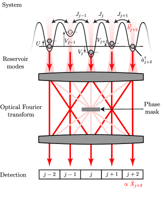
Here we focus on the idealized 1D Bose-Hubbard model subjected to continuous weak measurement [73, 74] to illustrate the possible dynamical steady states in many-body quantum systems. As depicted in Fig. 1 this model consists of: a 1D Bose-Hubbard chain (the system) dispersedly coupled to a transverse laser field (reservoir); measured via phase contrast imaging (optical homodyne detection); and with local tunneling strengths and on-site potentials that are dynamically adjusted based upon the measurement outcome (feedback). At time , the Bose-Hubbard chain is governed by the system Hamiltonian
expressed in terms of the bosonic field operators describing the creation of an atom at site and the number operator at site ; with positive real-valued tunneling strength between sites and ; on-site energy ; and interaction strength . The chemical potential is absent in this microcanonical ensemble study.
Measurement model. The system is coupled to the reservoir by the system-reservoir Hamiltonian
that describes a dispersive off-resonance interaction of light with two-level atoms, detected by homodyne measurement [75] or equivalently phase contrast imaging, shown in Fig. 1. Here, the bosonic field operator describes the addition of a photon into mode associated with lattice site (here we focus on an idealized case with mode functions associated one-to-one with lattice sites); captures the strength of the system-reservoir coupling; and the reservoir modes are each in the coherent state prior to interacting with the system. Physically this operator describes rotations in the - quadrature plane for each reservoir mode, in proportion to the local number of atoms. After interacting with the system for a time , the reservoir modes are projectively measured by optical homodyne measurement (in practice implemented by phase contrast imaging) giving access to the quadrature observables.
A strong measurement on the reservoir in effect affords a single weak measurement of the system observables with strength governed by , the reservoir field amplitude , and the measurement time . A measurement outcome
| (1) |
at time contains a contribution from the system observable’s instantaneous expectation value , along with a noise contribution from projectively measuring the reservoir coherent state . Here is a classical random variable with zero mean and variance . We consider an optical mode function consisting of a traveling pulse of light with extent , where is the speed of light. Converting from the continuum mode functions to this compact function introduces a factor of into the definition of the generalized measurement strength parameter. This leads to the generalized measurement strength parameter , defining the measurement noise and the back-action of this measurement on the system as described by the Kraus operator [76]
| (2) |
conditioned on the measurement outcomes . Given an initial state and a measurement outcome , the post-measurement state of the system is given by . As one might intuitively expect from a simple classical measurement, this gives a distribution of measurement outcomes with a width that decreases linearly with the system-reservoir coupling but as the square root of the measurement time and intensity of the probe field . In the following analysis, we consider the continuous limit of many such weak measurements, taking the time between subsequent measurements to be and applying measurements with a strength associated with a measurement time .
Feedback model. For sufficiently weak measurements, the quantum projection noise present in any individual measurement can greatly exceed the contribution of the instantaneous expectation value . As a result, we borrow from classical control theory [77], and derive an error signal from a temporal low-pass filter
| (3) |
applied to the direct measurement outcomes. This consists of an integrator with a low-frequency gain limit, with time constant . This filter retains the low frequency components of (containing contributions from both system dynamics and projection noise), but rejects the high frequency components (dominated by projection noise). Here we assume that the measurement time , implicitly making Eq. (3) a stochastic differential equation, see Ref. [41] for a more detailed discussion. The resulting error signal thus approximates the continuous measurement limit of a sequence of weak measurements of with measurement times regardless of the physical measurement time . Note that because this filter is applied in real time, will lag behind by , and we take in our simulations. Because the goal is neither to perform quantum state estimation nor to drive the system into a predefined state, we do not employ Kalman filter techniques [78].
Here we focus on possible dynamical steady states when this classical information is then fed back into the Hamiltonian in one of two ways. We shift either the on-site energy
| (4) |
in proportion to the local feedback signal (with gain ), or the tunneling
| (5) |
based on the difference along that link (with gain ). These two forms of feedback are the most simple physically realistic options: the potential simply shifts in proportion to the error signal; however, because negative tunneling is difficult to achieve, quadratic feedback is the most simple realistic feedback to the tunneling term. Both of these can be realized using quantum gas microscopes [79, 80] where a digital mirror device can locally control both the intensity of the lattice light (increasing or decreasing tunneling [81]) as well as changing the intensity on the lattice sites (altering the on-site potential [30]).
II Two-site lattice
The two-site Bose-Hubbard model with atoms can be recast as an angular momentum system with mappings , , and , that obey a dimensionless angular momentum commutation relation . This gives the Hamiltonian
| (6) |
where we have absorbed constant terms into an overall shift in the zero of energy and defined . This also results in the single filter equation
| (7) |
for and feedback equations
| (8) |
which are slightly adjusted with an additional factor of on the right-hand side of the filter equation, resulting from the details of the angular momentum mapping.
The on-site measurement outcomes at time can be re-expressed as
| (9) |
with contribution 111The factor of derives from combining two measurements of density into a single measurement of . from the instantaneous expectation value . As before, the noise is defined by a classical random variable with zero average , and variance . Back-action is described by the Kraus operator
| (10) |
Taken together, these expressions provide an equivalent formulation of the two-site system in the language of angular momentum.
Classical limit. The Heisenberg equations of motion in the large- limit (i.e., ignoring quantum fluctuations and thus measurement uncertainty) reduce to the classical equations of motion
| (14) |
where denotes the classical angular momentum vector, ignoring quantum fluctuations. Note that because the interaction enters via a quartic term in the Hamiltonian, it enters the classical equations of motion nonlinearly. Thus in order to properly compare systems with different , we keep fixed to a constant value. Similarly, since the potential and tunneling feedback terms behave like effective fourth- and sixth-order terms in the Hamiltonian, respectively, we must also keep and fixed to constant values.
Tunneling causes the macroscopic spin vector to precess around ; a potential imbalance leads to precession around ; and the non-linear interaction term effectively drives precession around with angular frequency in proportion to . Figure 2(a) plots the energy [from Eq. (6)] and trajectories [from Eq. (14)] for , as a function of the polar angles and with respect to an aligned spherical coordinate system ( in the -direction). The displayed trajectories illustrate the two classes of orbits. (1) Near (i.e., ), the phase exhibits running solutions [83, 84] orbiting around : Josephson oscillations (JO). (2) For larger , closed orbits around , and correspond to oscillations about a density imbalanced excited state [85]: macroscopic self trapping (MST), present only for . For the two MST solutions merge to form a second stable JO fixed point at .
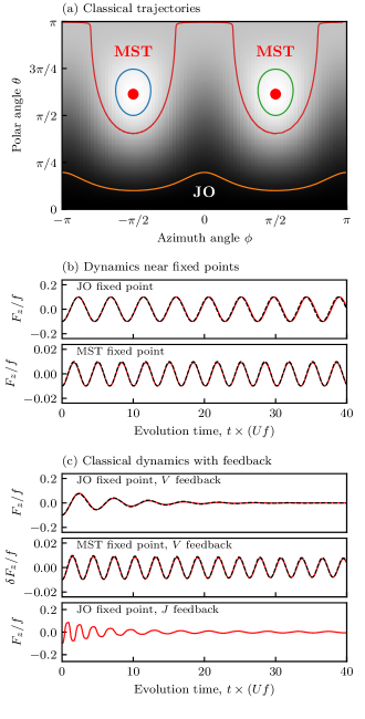
Linearized dynamics. The impact of feedback is most clearly understood by first linearizing the dynamics around each of the stable fixed points of the JO and MST orbits, in general giving elliptical orbits. The displacements each obey second-order differential equations such as
| (15) |
describing motion in an effective harmonic potential, with angular frequencies
for the JO and MST points respectively. For , the feedback described by Eq. (8) becomes proportional to and shifts the location of the fixed points (potentially even eliminating them entirely), as well as altering the frequency and ellipticity of the orbits. Still, the form of the differential equations is unchanged: no damping. In the above example, conventional damping would arise from an additional friction term , and more generally damping (or anti-damping) will occur only when odd and even derivatives are mixed. In our case, mixes these derivatives when , changing the relationship between and according to Eq. (7), thus changing the effect of on Eqs. (8,14). The effect of feedback can be quantified in linear response about both the JO and the MST fixed points, allowing us to derive a damping rate in each case, in the limit of weak damping , where is the angular frequency of the relevant fixed point. In this limit, the damping rates are , with the most effective damping when , and where the strength governs the system dependence of the feedback. For feedback in the potential, the resulting strengths are
showing that, depending on the sign of , the system can be damped effectively. Focusing on the case of positive interactions and positive base tunneling , either only the JO fixed point is stable (), only the MST fixed points are stable (), or both types of fixed points are stable ().
In contrast, for feedback in the tunneling channel, the quadratic response leads to very slow damping as the density-balanced JO fixed point is approached, i.e., at the JO fixed point, , and the linear contribution to is zero. Thus, only the MST state has damping or anti-damping in linear response, and for the physical sign of the gain coefficient , this results in anti-damping.
Fluctuations. Although the classical limit omits quantum fluctuations (by assuming a spin-coherent state), it need not omit measurement back action. A prescription similar to that of Ref. [40] for coherent states gives a final state conditioned on the random variable
| (16) |
for measurements of described by Eq. (9), where is defined with respect to . This prescription takes an initial spin coherent state, then applies the Kraus operator; because the resulting state is not necessarily a spin-coherent state, we find the coherent state with the largest overlap as the updated state. The core message of this expression is that is updated as informed by the measurement outcome, but for initial states nearly polarized along , the state is nearly unaltered. Physically, this is expected because we are working at fixed total angular momentum , and a state already polarized along cannot become more polarized.
Lastly, equating Eqs. (9) and (16) suggests an optimal measurement strength for which the true value of following the measurement [Eq. (9)] is equal to the measurement outcome [Eq. (16)], i.e., the measurement outcome accurately reflects the new state of the system. This occurs only for an optimal measurement strength , that would be selected to yield optimal performance near the desired fixed point. We also note that with Eqs. (9) and (16), this implies that for the optimal measurement strength, the measurement noise and back-action both scale like , fractionally going to zero in the limit as one would expect.
The low-pass filter from which we derive the error signal has time-constant , which plays the role of an effective measurement time. Assuming no delay between measurements, this implies an individual-measurement coupling , so that the measurements which take place in the time interval give a single average outcome with the optimal strength .
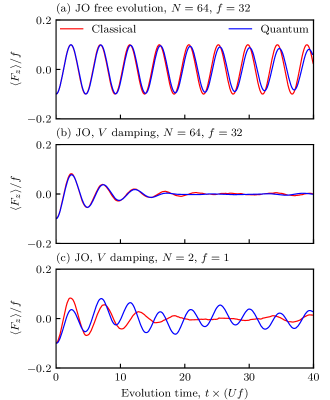
Quantum double well. With these basic insights from the classical model in mind, we compare to a quantum-trajectories stochastic Schrödinger equation simulation of this double-well problem, including all effects of back-action resulting from measurement to the classical spin model, including measurement noise and back-action. Figure 3(a) shows the coherent evolution of a spin coherent state with or , according to the classical spin model (red) and the quantum simulation (blue), with nearly perfect overlap. The agreement continues to improve with increasing , as neglecting quantum fluctuations becomes an increasingly good approximation. This overlap persists in Fig. 3(b) which includes the effects of measurement, back-action, and feedback, again showing good correspondence between the classical and quantum models. Lastly, as the number is reduced from to (and is correspondingly increased by a factor of to keep ), neglecting fluctuations becomes a very poor approximation, and the classical and quantum trajectories deviate.
The classical-limit modeling provided valuable insight in guiding parameter selection even for quantum systems: (1) feedback can change the dynamical steady state by introducing effective potentials; and (2) the optimal filter time is inversely proportional to the dynamical time scale of excitations in the measurement channel. A basic intuition for the latter point comes from a continuously monitored classical harmonic oscillator. The measured position converts into knowledge of momentum one-quarter period later, allowing a time-delayed feedback force to reduce that known velocity. In the present case, in the lowpass filter gives the same outcome by introducing a phase shift for signals with angular frequency . We certainly expect that more complex filters, proportional-integral-differential (PID) or Kalman [78] filters for example, would give improved performance.
III Extended lattice
In this section, we extend our analysis to the case of small one-dimensional Bose-Hubbard chains. Unlike the case of two sites, there is no angular momentum map, and the appropriate mean-field description is a discrete Gross-Pitaevskii equation, similar to that discussed in Refs. [40, 41]. Here, we focus on the quantum region by considering states with mean densities of just a few particles per-site and studying the system’s behavior numerically using a quantum trajectories approach [86, 87, 88]. Correspondingly, the fluctuations in all figures are a result of sampling error. We will also consider a range of target density distributions, in which the error signal derives from the difference between the observation and the target. Throughout, we will express everything in units where the interaction strength . Recent closely-related work investigates preparing similar Mott-like states via global measurements rather than the local measurements considered here [39].
Feedback models. We consider two possible tunneling feedback schemes. The first is the nearest-neighbor approach introduced in Eq. (5). The second, the “imbalance approach”, uses highly non-local information, and relies instead on imbalances between the left and right sides of the system. For the double-well system considered earlier, these two schemes are identical. The tunneling strengths are, respectively,
| (17) |
| (18) |
where
| (19) | |||||
and indicates the target occupation number of site . Since the tunneling strength without feedback is and measurement occurs in the number basis, this means that the target state will be an evolution-free fixed point in the absence of feedback induced by noise from the measurements. Given the structure of the imbalance approach, which entails separating the system into left and right sides, we will consider open boundary conditions when discussing state preparation.
The purpose of the imbalance approach is to take advantage of the global knowledge of the target state, knowledge that is not used in the nearest-neighbor approach. For example, consider the scenario in which the target state is and the system is in the state . In this case, the nearest-neighbor approach will only initially turn on the tunneling between the first two sites and gradually turn on the other tunneling terms from left to right as the bosons move to the left. In contrast, the imbalance approach will turn on all tunneling terms and begin to transfer atoms from the right side of the system to the left. However, the use of this more global knowledge comes at a cost to the feedback uncertainty. Since involves a sum of different measurement records, the resulting uncertainty will be enhanced by a factor of . As a result, there is a trade-off between using global knowledge and the uncertainty in the feedback. Finally, we will discuss these two feedback approaches in terms of a continuous measurement rate , where and we use in our numerical simulations.
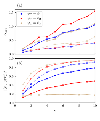
State preparation. We compare the performance of these two approaches for three different target states: , and . We fix the filter time and the evolution time 222The extra time is to allow for an initialization of before the feedback starts being applied at . in units of and examine the behavior of the final target state overlap as a function of and . For each trajectory, we initialize the system in a Haar random state. While we could consider the steady-state behavior of this system, from the perspective of creating a target state in a physical system, it is more useful to consider the finite-time behavior.
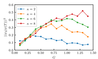
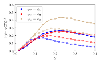
Fig. 4 illustrates the target state overlap for at different values of and using the nearest-neighbor approach. The behavior for other target states and the imbalance approach are qualitatively similar. For all values of the measurement strength , we see that there is an optimal choice of the gain for which the overlap is maximized. This optimal value of the gain represents a balance between the need to direct the system to the desired target state quickly and the fact that measurement uncertainty can lead to “errors” in the application of the feedback. We identify the optimal value of the gain and the corresponding target state overlap for the different target states and measurement strengths in Fig. 5. Several trends can be identified in the optimal feedback behavior.
The first trend is that the optimal gain grows linearly with the measurement strength. This reflects the fact that stronger measurements correspond to more accurate knowledge of the system’s state, so the system can be more strongly driven to the target state without making errors due to the measurement uncertainty. Additionally, the gain must increase with the measurement strength to avoid quantum Zeno effects, i.e., the dynamics due to the feedback must become sufficiently fast so that the repeated weak measurements do not effectively become a strong measurement before the system can evolve coherently.
The second trend is that optimal gain is larger for the nearest-neighbor approach than the imbalance approach. This is most likely a result of the fact that the uncertainty is larger for the imbalance approach. Since the imbalance approach uses 5 measurements for each tunneling link while the nearest-neighbor approach uses 2, the relative uncertainties in the tunneling strength differ by roughly a factor of 2.5 333for white noise with standard deviation , the mean and standard deviation of are and , respectively, hence the factor of rather than , which is consistent with the observed behavior.
The third trend is that for the parameters and target states considered, the imbalance approach performs much better than the nearest-neighbor approach. The nearest-neighbor approach performs better the more homogeneous the target state is. However, this begins to change at lower values of the measurement strength, where the target state overlap sharply begins to fall. This is a consequence of the fact that, at sufficiently small measurement strengths, the uncertainty in the measurement—and therefore the feedback signal—overwhelms the useful information. Since the imbalance approach involves more measurements, this behavior occurs earlier than for the nearest-neighbor approach.
Nearby state preparation. For larger systems, the effect of the increased uncertainty that comes with the imbalance approach becomes far more important. A natural approach to avoid this issue is to use a more hierarchical approach to the application of feedback. When the system starts initially far from the desired target state, a more global approach to feedback should be used. As the system gets closer to the target state according to the measurement record, then increasingly local feedback approaches can be used.
While the systems we can consider numerically are too small to apply such a hierarchical feedback approach, we can explore how the performance of the two feedback approaches can change if the system is already closer to the target state. To do so, we consider initial states whose only difference from the target state is that a single boson has been moved one site away. Additionally, we allow the feedback to be applied for only one unit of time after the initialization of the measurement record (which requires time ), reflecting the fact that the local feedback would be applied for a shorter time in this hierarchical approach. The results of our numerics are shown in Fig. 6 for , demonstrating that the nearest-neighbor approach performs better when the system is already close to the desired state due to the reduced uncertainty in the feedback. Note that this is in spite of the fact that the nearest-neighbor approach will initially turn on three coupling terms while the imbalance approach will turn on only one in the absence of measurement uncertainty.
Symmetry-breaking transition. The emergence of phase transitions via feedback has been investigated in a variety of diverse contexts [42, 43, 44, 45, 46, 41, 47, 48, 49], and here we explore a symmetry-breaking transition in an extended Hubbard chain. To observe this, we will consider a six-site lattice with periodic boundaries whose tunneling feedback drives the system towards the states or . Due to the periodic boundary conditions and type of symmetry breaking, the left-right imbalance approach is not applicable, so we consider a generalization of the nearest-neighbor feedback. In particular, the tunneling feedback is
| (20a) | |||
| (20b) |
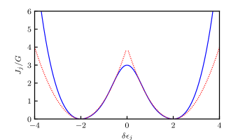
with . This is essentially a product of the tunneling feedback in Eq. (18) for . The Gaussian term is included in order to increase the tunneling for compared to just the quartic potential so that it is comparable to the corresponding tunneling when only one of the two aforementioned states is a target state. This will serve as a barrier which hinders the system from moving from to and vice-versa (see Fig. 7).
An additional important feature to note for this choice of feedback is that these are not the only two states which will lead to small tunneling. States of the form can also be relatively stable. While there is one pair of sites with large tunneling, this pair of sites has no bosons, so the large hopping is not sufficient on its own to change the state. However, there are two factors that can make such states unfavorable. The first is that the creation of these states requires four bosons on a single site, which is energetically unfavorable. The second is that once measurement-induced fluctuations cause one of the bosons at sites with two bosons to move into an empty site, the boson will quickly move to the next site.
In order to investigate the symmetry-breaking behavior of this feedback, we consider the behavior of the steady-state density matrix for fixed as a function of , which we obtain via a combination of ensemble and ergodic averaging. Additionally, we define an effective Hamiltonian according to . In analogy to equilibrium systems, a symmetry breaking phase will occur when the two lowest energy levels of become gapped from the rest of the spectrum. In terms of , the two corresponding states will have a much larger probability than the rest of the eigenstates, and the gap in describes the exponential suppression in probability of these other eigenstates. Hence in the absence of a gap, no particular configuration is favored, and the system appears disordered.
Fig. 8 plots the eigenvalues of as a function of for using the initial state , which will prefer both symmetry-breaking states equally, although we expect the same steady state for Haar random initial states. We see that an effective gap opens for a range of , with two effective energies much smaller than the rest. As expected, these two eigenvectors correspond approximately to and , while the other possible stable states (e.g., ) are not strongly occupied. Additionally, as this gap increases, the auto-correlation times increase, necessitating more sampling for larger gaps. This corresponds to the fact that when the system is in either of the two symmetry-broken states, the feedback makes it difficult to leave this state, so the system spends a long time in the same state, thus slowing down the ergodic sampling of . In the limit of large , even small fluctuations will drastically modify , preventing the system from preferring any particular state and causing the gap to close.
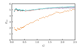
As is increased, this gap eventually closes and does not reopen. Physically, this is because in the limit of large , the hopping becomes very large, so small fluctuations in the measurements lead to large fluctuations in the hopping, preventing the system from preferring any given state. This is qualitatively similar to an infinite temperature limit in which no particular state is energetically preferred. In the limit of small , the gap similarly closes because the measurement strength overwhelms the feedback, causing the system to relax to a random number state. The start of this closure can be observed in Fig. 8, although due to the quantum Zeno effect, identifying the steady state for smaller values of becomes numerically prohibitive as it requires increasingly long relaxation times.
IV Outlook
This study combines concepts from many-body physics with the techniques of quantum control and feedback to create and characterize low entropy many-body dynamical steady states. Creating such dynamical steady state in the laboratory environment hinges on exploring the implication of experimental realities, for example: What are the consequences of imperfect detection? Of limited spatial resolution? What is the impact of limited feedback bandwidth? Real implementation must face these questions head-on.
From a foundational perspective, it remains to be seen if there exist dynamical steady states which are forbidden in associated thermal equilibrium systems. For example, nonreciprocal couplings can be realized using feedback, which can lead to rich non-equilibrium phenomena [91, 92, 93, 94]. Alternatively, feedback that is non-local in time can be used to engineer non-Markovian baths even though the measurements themselves are Markovian. Similarly, even with local measurements of density, non-local feedback can emulate aspects of long-range potentials [37]. Stochastic descriptions such as ours can be reframed in terms of the so-called feedback master equation [95], in which the time delay introduced by the low pass filter introduces non-Markovian terms that cannot be described in a Lindblad form. This at least provides the opportunity for creating dynamics and steady states that are not achievable using realistic Lindblad terms. Moreover, even if the steady state may look thermal, its linear response may still violate the fluctuation-dissipation theorem [96, 97], indicating the persistence of non-equilibrium features. Additionally, new types of dynamics are possible when the bosons include a spin degree of freedom, such as quantum Zeno-like effects which can emerge if one spin state is subjected to stronger measurements than the other.
While we have demonstrated how the use of non-local feedback can be employed to prepare desired target states more efficiently than local feedback, this was done for the relatively simple case of Mott-like number states. An interesting next direction, then, is to consider preparing more complex states, such as superfluid-like states with long-range coherences. By adding density modulations through the use of non-local feedback as we did for the number states, this opens the possibility of preparing supersolid and supersolid-like states [98, 99, 100, 101]. More broadly, this would provide further insight into how the use of measurement and feedback affects the ability to realize intrinsically quantum dynamics.
Although we have illustrated how a symmetry-breaking phase transition may in principal emerge due to measurement and feedback in a many-body quantum system, several open questions remain. Here, our analysis has been restricted to small 1D chains, so an important question is whether this corresponds to a phase transition in the thermodynamic limit. Even if it does not exist in 1D, an analogous transition may exist in higher-dimensional systems. Additionally, understanding the behavior of critical phenomena in these systems is another important direction, such as whether they are equivalent to a quantum phase transition, a classical phase transition, or something entirely different. In Ref. [46], it was shown that in zero-dimensional systems, modifying the form of non-Markovian feedback can lead to changes in the critical exponents of the phase transition, so similar phenomena may arise in a many-body context as well.
A natural direction to explore in order to investigate these questions are measurement-induced phase transitions, which have been the subject of intense theoretical research in recent years and are defined by the scaling behavior of the entanglement entropy [102, 103, 104, 105, 106, 107, 108, 109, 110, 111, 112, 113, 114, 115, 116, 117, 118], with recent initial experimental evidence [119]. Aside from the key difference that these systems are not subject to feedback, these often involve coherent evolution defined by random unitary circuits and strong measurements, although similar behavior has been shown to emerge for weak measurements as well [114, 115, 116, 117, 118]. A natural question is how these phase transitions can be modified through different applications of feedback; will the phase transition only shift, or can qualitatively new physics emerge?
Another promising approach to exploring the above questions is to investigate the similarities that systems subject to measurement and feedback have with driven-dissipative systems, which are systems that are subjected to coherent drive and incoherent dissipation that have been studied extensively in a variety of contexts [10, 11, 12, 13, 14, 15, 16, 18, 19, 20, 17, 120, 121, 122, 123, 124, 125, 126, 127, 128, 129, 130, 131, 132, 133, 134, 93, 135, 21, 136]. From an abstract standpoint, these two types of systems are very similar, with dissipation playing a role analogous to continuous measurements and drive playing a role analogous to the feedback. As a result, insights or techniques from studying one type of system can lead to insights in the other. For example, phase transitions in driven-dissipative systems have been studied extensively using a Keldysh-Schwinger and functional integral formalism [122, 123, 124, 125, 126, 127, 128, 129, 130, 93, 131], so it is important to explore how these same techniques can be applied to systems subject to measurement and feedback. Similarly, effective classical equilibrium criticality is observed generically in many driven-dissipative phase transitions [127, 128, 129], with some important exceptions [130, 132, 93, 131], so measurement-feedback systems may provide new avenues to realize novel forms of non-equilibrium criticality and quantum criticality. Moreover, recent research indicates that dissipative phase transitions and measurement-induced phase transitions need not coincide [136], which means that measurement-feedback phase transitions may similarly lead to distinctive forms of criticality.
Acknowledgements.
We benefited greatly from conversations with H. M. Hurst, J. K. Thompson, J. Ye, L. Walker, R. Lena, A. Daley, L. P. García-Pintos, S. Guo, and E. Altuntas. We appreciate the careful reading from S. Lieu and D. Barberena. J.T.Y. was supported by the NIST NRC Research Postdoctoral Associateship Award. A.V.G. acknowledges funding by DARPA SAVaNT ADVENT, AFOSR, ARO MURI, AFOSR MURI, U.S. Department of Energy Award No. DE-SC0019449, NSF PFCQC program, DoE ASCR Accelerated Research in Quantum Computing program (Award No. DE-SC0020312), and DoE ASCR Quantum Testbed Pathfinder program (Award No. DE-SC0019040). This work was supported by NIST. Analysis was performed in part on the NIST Raritan HPC cluster.References
- Cassidy et al. [2011] A. C. Cassidy, C. W. Clark, and M. Rigol, Generalized Thermalization in an Integrable Lattice System, Phys. Rev. Lett. 106, 140405 (2011).
- Langen et al. [2015] T. Langen, S. Erne, R. Geiger, B. Rauer, T. Schweigler, M. Kuhnert, W. Rohringer, I. E. Mazets, T. Gasenzer, and J. Schmiedmayer, Experimental observation of a generalized Gibbs ensemble, Science 348, 207 (2015).
- Ilievski et al. [2016] E. Ilievski, M. Medenjak, T. Prosen, and L. Zadnik, Quasilocal charges in integrable lattice systems, Journal of Statistical Mechanics: Theory and Experiment 2016, 064008 (2016).
- Calabrese et al. [2016] P. Calabrese, F. H. L. Essler, and G. Mussardo, Introduction to ‘quantum integrability in out of equilibrium systems’, Journal of Statistical Mechanics: Theory and Experiment 2016, 064001 (2016).
- Vidmar and Rigol [2016] L. Vidmar and M. Rigol, Generalized Gibbs ensemble in integrable lattice models, Journal of Statistical Mechanics: Theory and Experiment 2016, 064007 (2016).
- Mori et al. [2018] T. Mori, T. N. Ikeda, E. Kaminishi, and M. Ueda, Thermalization and prethermalization in isolated quantum systems: a theoretical overview, Journal of Physics B: Atomic, Molecular and Optical Physics 51, 112001 (2018).
- Kinoshita et al. [2006] T. Kinoshita, T. Wenger, and D. S. Weiss, A quantum Newton’s cradle, Nature 440, 900 (2006).
- Gring et al. [2012] M. Gring, M. Kuhnert, T. Langen, T. Kitagawa, B. Rauer, M. Schreitl, I. Mazets, D. A. Smith, E. Demler, and J. Schmiedmayer, Relaxation and Prethermalization in an Isolated Quantum System, Science 337, 1318 (2012).
- Tang et al. [2018] Y. Tang, W. Kao, K.-Y. Li, S. Seo, K. Mallayya, M. Rigol, S. Gopalakrishnan, and B. L. Lev, Thermalization near Integrability in a Dipolar Quantum Newton’s Cradle, Phys. Rev. X 8, 021030 (2018).
- Diehl et al. [2008] S. Diehl, A. Micheli, A. Kantian, B. Kraus, H. P. Büchler, and P. Zoller, Quantum states and phases in driven open quantum systems with cold atoms, Nat. Phys. 4, 878 (2008).
- Szymańska et al. [2007] M. H. Szymańska, J. Keeling, and P. B. Littlewood, Mean-field theory and fluctuation spectrum of a pumped decaying Bose-Fermi system across the quantum condensation transition, Phys. Rev. B 75, 195331 (2007).
- Yi et al. [2012] W. Yi, S. Diehl, A. J. Daley, and P. Zoller, Driven-dissipative many-body pairing states for cold fermionic atoms in an optical lattice, New J. Phys. 14, 055002 (2012).
- Bardyn et al. [2013] C.-E. Bardyn, M. A. Baranov, C. V. Kraus, E. Rico, A. İmamoğlu, P. Zoller, and S. Diehl, Topology by dissipation, New J. Phys. 15, 085001 (2013).
- Baumann et al. [2010] K. Baumann, C. Guerlin, F. Brennecke, and T. Esslinger, Dicke quantum phase transition with a superfluid gas in an optical cavity, Nature (London) 464, 1301 (2010).
- Carr et al. [2013] C. Carr, R. Ritter, C. G. Wade, C. S. Adams, and K. J. Weatherill, Nonequilibrium Phase Transition in a Dilute Rydberg Ensemble, Phys. Rev. Lett. 111, 113901 (2013).
- Malossi et al. [2014] N. Malossi, M. M. Valado, S. Scotto, P. Huillery, P. Pillet, D. Ciampini, E. Arimondo, and O. Morsch, Full Counting Statistics and Phase Diagram of a Dissipative Rydberg Gas, Phys. Rev. Lett. 113, 023006 (2014).
- Jin et al. [2016] J. Jin, A. Biella, O. Viyuela, L. Mazza, J. Keeling, R. Fazio, and D. Rossini, Cluster Mean-Field Approach to the Steady-State Phase Diagram of Dissipative Spin Systems, Phys. Rev. X 6, 031011 (2016).
- Rodriguez et al. [2017] S. R. K. Rodriguez, W. Casteels, F. Storme, N. Carlon Zambon, I. Sagnes, L. Le Gratiet, E. Galopin, A. Lemaître, A. Amo, C. Ciuti, and J. Bloch, Probing a Dissipative Phase Transition via Dynamical Optical Hysteresis, Phys. Rev. Lett. 118, 247402 (2017).
- Fitzpatrick et al. [2017] M. Fitzpatrick, N. M. Sundaresan, A. C. Y. Li, J. Koch, and A. A. Houck, Observation of a Dissipative Phase Transition in a One-Dimensional Circuit QED Lattice, Phys. Rev. X 7, 011016 (2017).
- Dogra et al. [2019] N. Dogra, M. Landini, K. Kroeger, L. Hruby, T. Donner, and T. Esslinger, Dissipation-induced structural instability and chiral dynamics in a quantum gas, Science 366, 1496 (2019).
- Scarlatella et al. [2021] O. Scarlatella, A. A. Clerk, R. Fazio, and M. Schiró, Dynamical Mean-Field Theory for Markovian Open Quantum Many-Body Systems, Phys. Rev. X 11, 031018 (2021).
- Wu et al. [1991] W. Wu, B. Ellman, T. F. Rosenbaum, G. Aeppli, and D. H. Reich, From classical to quantum glass, Phys. Rev. Lett. 67, 2076 (1991).
- Gopalakrishnan et al. [2011] S. Gopalakrishnan, B. L. Lev, and P. M. Goldbart, Frustration and Glassiness in Spin Models with Cavity-Mediated Interactions, Phys. Rev. Lett. 107, 277201 (2011).
- Altman and Vosk [2015] E. Altman and R. Vosk, Universal Dynamics and Renormalization in Many-Body-Localized Systems, Annual Review of Condensed Matter Physics 6, 383 (2015).
- Nandkishore and Huse [2015] R. Nandkishore and D. A. Huse, Many-Body Localization and Thermalization in Quantum Statistical Mechanics, Annu. Rev. Condens. Matter Phys. 6, 15 (2015).
- Gogolin and Eisert [2016] C. Gogolin and J. Eisert, Equilibration, thermalisation, and the emergence of statistical mechanics in closed quantum systems, Reports on Progress in Physics 79, 056001 (2016).
- Alet and Laflorencie [2018] F. Alet and N. Laflorencie, Many-body localization: An introduction and selected topics, Comptes Rendus Physique 19, 498 (2018).
- Abanin et al. [2019] D. A. Abanin, E. Altman, I. Bloch, and M. Serbyn, Colloquium: Many-body localization, thermalization, and entanglement, Rev. Mod. Phys. 91, 021001 (2019).
- Schreiber et al. [2015] M. Schreiber, S. S. Hodgman, P. Bordia, H. P. Luschen, M. H. Fischer, R. Vosk, E. Altman, U. Schneider, and I. Bloch, Observation of many-body localization of interacting fermions in a quasirandom optical lattice, Science 349, 842 (2015).
- Choi et al. [2016] J.-y. Choi, S. Hild, J. Zeiher, P. Schauß, A. Rubio-Abadal, T. Yefsah, V. Khemani, D. A. Huse, I. Bloch, and C. Gross, Exploring the many-body localization transition in two dimensions, Science 352, 1547 (2016).
- Smith et al. [2016] J. Smith, A. Lee, P. Richerme, B. Neyenhuis, P. W. Hess, P. Hauke, M. Heyl, D. A. Huse, and C. Monroe, Many-body localization in a quantum simulator with programmable random disorder, Nat. Phys. 12, 907 (2016).
- Roushan et al. [2017] P. Roushan, C. Neill, J. Tangpanitanon, V. M. Bastidas, A. Megrant, R. Barends, Y. Chen, Z. Chen, B. Chiaro, A. Dunsworth, A. Fowler, B. Foxen, M. Giustina, E. Jeffrey, J. Kelly, E. Lucero, J. Mutus, M. Neeley, C. Quintana, D. Sank, A. Vainsencher, J. Wenner, T. White, H. Neven, D. G. Angelakis, and J. Martinis, Spectroscopic signatures of localization with interacting photons in superconducting qubits, Science 358, 1175 (2017).
- Guo et al. [2021] Q. Guo, C. Cheng, Z.-H. S. Z. Song, H. Li, Z. Wang, W. Ren, H. Dong, D. Zheng, Y.-R. Zhang, R. Mondaini, H. Fan, and H. Wang, Observation of energy-resolved many-body localization, Nat. Phys. 17, 234 (2021).
- Lloyd and Slotine [2000] S. Lloyd and J.-J. E. Slotine, Quantum feedback with weak measurements, Phys. Rev. A 62, 012307 (2000).
- Thomsen et al. [2002] L. K. Thomsen, S. Mancini, and H. M. Wiseman, Spin squeezing via quantum feedback, Phys. Rev. A 65, 061801(R) (2002).
- Shankar et al. [2019] A. Shankar, G. P. Greve, B. Wu, J. K. Thompson, and M. Holland, Continuous Real-Time Tracking of a Quantum Phase Below the Standard Quantum Limit, Phys. Rev. Lett. 122, 233602 (2019).
- Muschik et al. [2013] C. A. Muschik, K. Hammerer, E. S. Polzik, and I. J. Cirac, Quantum Teleportation of Dynamics and Effective Interactions between Remote Systems, Phys. Rev. Lett. 111, 020501 (2013).
- Muñoz-Arias et al. [2020a] M. H. Muñoz-Arias, P. M. Poggi, P. S. Jessen, and I. H. Deutsch, Simulating Nonlinear Dynamics of Collective Spins via Quantum Measurement and Feedback, Phys. Rev. Lett. 124, 110503 (2020a).
- Wu and Eckardt [2021] L.-N. Wu and A. Eckardt, Cooling and state preparation in an optical lattice via Markovian feedback control (2021), arXiv:2106.03883 [cond-mat.quant-gas] .
- Hurst and Spielman [2019] H. M. Hurst and I. B. Spielman, Measurement-induced dynamics and stabilization of spinor-condensate domain walls, Phys. Rev. A 99, 053612 (2019).
- Hurst et al. [2020] H. M. Hurst, S. Guo, and I. B. Spielman, Feedback induced magnetic phases in binary Bose-Einstein condensates, Phys. Rev. Research 2, 043325 (2020).
- Grimsmo et al. [2014] A. L. Grimsmo, A. S. Parkins, and B.-S. Skagerstam, Rapid steady-state convergence for quantum systems using time-delayed feedback control, New Journal of Physics 16, 065004 (2014).
- Kopylov et al. [2015] W. Kopylov, C. Emary, E. Schöll, and T. Brandes, Time-delayed feedback control of the dicke–hepp–lieb superradiant quantum phase transition, New Journal of Physics 17, 013040 (2015).
- Mazzucchi et al. [2016] G. Mazzucchi, S. F. Caballero-Benitez, D. A. Ivanov, and I. B. Mekhov, Quantum optical feedback control for creating strong correlations in many-body systems, Optica 3, 1213 (2016).
- Muñoz-Arias et al. [2020b] M. H. Muñoz-Arias, I. H. Deutsch, P. S. Jessen, and P. M. Poggi, Simulation of the complex dynamics of mean-field -spin models using measurement-based quantum feedback control, Phys. Rev. A 102, 022610 (2020b).
- Ivanov et al. [2020a] D. A. Ivanov, T. Y. Ivanova, S. F. Caballero-Benitez, and I. B. Mekhov, Feedback-Induced Quantum Phase Transitions Using Weak Measurements, Phys. Rev. Lett. 124, 010603 (2020a).
- Kroeger et al. [2020] K. Kroeger, N. Dogra, R. Rosa-Medina, M. Paluch, F. Ferri, T. Donner, and T. Esslinger, Continuous feedback on a quantum gas coupled to an optical cavity, New Journal of Physics 22, 033020 (2020).
- Ivanov et al. [2020b] D. A. Ivanov, T. Y. Ivanova, S. F. Caballero-Benitez, and I. B. Mekhov, Cavityless self-organization of ultracold atoms due to the feedback-induced phase transition, Sci. Rep. 10, 10550 (2020b).
- Ivanov et al. [2021] D. A. Ivanov, T. Y. Ivanova, S. F. Caballero-Benitez, and I. B. Mekhov, Tuning the universality class of phase transitions by feedback: Open quantum systems beyond dissipation, Phys. Rev. A 104, 033719 (2021).
- Happer [1972] W. Happer, Optical Pumping, Rev. Mod. Phys. 44, 169 (1972).
- Lett et al. [1988] P. D. Lett, R. N. Watts, C. I. Westbrook, W. D. Phillips, P. L. Gould, and H. J. Metcalf, Observation of Atoms Laser Cooled below the Doppler Limit, Phys. Rev. Lett. 61, 169 (1988).
- Shor [1995] P. W. Shor, Scheme for reducing decoherence in quantum computer memory, Phys. Rev. A 52, R2493 (1995).
- Terhal [2015] B. M. Terhal, Quantum error correction for quantum memories, Rev. Mod. Phys. 87, 307 (2015).
- Devitt et al. [2013] S. J. Devitt, W. J. Munro, and K. Nemoto, Quantum error correction for beginners, Reports Prog. Phys. 76, 076001 (2013).
- Giovannetti et al. [2011] V. Giovannetti, S. Lloyd, and L. Maccone, Advances in quantum metrology, Nat. Photonics 5, 222 (2011).
- Degen et al. [2017] C. L. Degen, F. Reinhard, and P. Cappellaro, Quantum sensing, Rev. Mod. Phys. 89, 035002 (2017).
- Walls [1983] D. F. Walls, Squeezed states of light, Nature (London) 306, 141 (1983).
- Kitagawa and Ueda [1993] M. Kitagawa and M. Ueda, Squeezed spin states, Phys. Rev. A 47, 5138 (1993).
- Schleier-Smith et al. [2010] M. H. Schleier-Smith, I. D. Leroux, and V. Vuletić, States of an Ensemble of Two-Level Atoms with Reduced Quantum Uncertainty, Phys. Rev. Lett. 104, 073604 (2010).
- Hosten et al. [2016] O. Hosten, N. J. Engelsen, R. Krishnakumar, and M. A. Kasevich, Measurement noise 100 times lower than the quantum-projection limit using entangled atoms, Nature 529, 505 (2016).
- Cox et al. [2016] K. C. Cox, G. P. Greve, J. M. Weiner, and J. K. Thompson, Deterministic Squeezed States with Collective Measurements and Feedback, Phys. Rev. Lett. 116, 093602 (2016).
- Korotkov [2001] A. N. Korotkov, Selective quantum evolution of a qubit state due to continuous measurement, Phys. Rev. B 63, 115403 (2001).
- Ahn et al. [2002] C. Ahn, A. C. Doherty, and A. J. Landahl, Continuous quantum error correction via quantum feedback control, Phys. Rev. A 65, 042301 (2002).
- Sarovar et al. [2004] M. Sarovar, C. Ahn, K. Jacobs, and G. J. Milburn, Practical scheme for error control using feedback, Phys. Rev. A 69, 052324 (2004).
- Dür et al. [2014] W. Dür, M. Skotiniotis, F. Fröwis, and B. Kraus, Improved Quantum Metrology Using Quantum Error Correction, Phys. Rev. Lett. 112, 080801 (2014).
- Kessler et al. [2014] E. M. Kessler, I. Lovchinsky, A. O. Sushkov, and M. D. Lukin, Quantum Error Correction for Metrology, Phys. Rev. Lett. 112, 150802 (2014).
- Arrad et al. [2014] G. Arrad, Y. Vinkler, D. Aharonov, and A. Retzker, Increasing Sensing Resolution with Error Correction, Phys. Rev. Lett. 112, 150801 (2014).
- Unden et al. [2016] T. Unden, P. Balasubramanian, D. Louzon, Y. Vinkler, M. B. Plenio, M. Markham, D. Twitchen, A. Stacey, I. Lovchinsky, A. O. Sushkov, M. D. Lukin, A. Retzker, B. Naydenov, L. P. McGuinness, and F. Jelezko, Quantum Metrology Enhanced by Repetitive Quantum Error Correction, Phys. Rev. Lett. 116, 230502 (2016).
- Sekatski et al. [2017] P. Sekatski, M. Skotiniotis, J. Kołodyński, and W. Dür, Quantum metrology with full and fast quantum control, Quantum 1, 27 (2017).
- Reiter et al. [2017] F. Reiter, A. S. Sørensen, P. Zoller, and C. A. Muschik, Dissipative quantum error correction and application to quantum sensing with trapped ions, Nat. Commun. 8, 1822 (2017).
- Zhou et al. [2018] S. Zhou, M. Zhang, J. Preskill, and L. Jiang, Achieving the Heisenberg limit in quantum metrology using quantum error correction, Nat. Commun. 9, 78 (2018).
- Layden et al. [2019] D. Layden, S. Zhou, P. Cappellaro, and L. Jiang, Ancilla-Free Quantum Error Correction Codes for Quantum Metrology, Phys. Rev. Lett. 122, 040502 (2019).
- Jacobs and Steck [2006] K. Jacobs and D. A. Steck, A straightforward introduction to continuous quantum measurement, Contemp. Phys. 47, 279 (2006).
- Clerk et al. [2010] A. A. Clerk, M. H. Devoret, S. M. Girvin, F. Marquardt, and R. J. Schoelkopf, Introduction to quantum noise, measurement, and amplification, Rev. Mod. Phys. 82, 1155 (2010).
- Hush et al. [2013] M. R. Hush, S. S. Szigeti, A. R. R. Carvalho, and J. J. Hope, Controlling spontaneous-emission noise in measurement-based feedback cooling of a Bose–Einstein condensate, New Journal of Physics 15, 113060 (2013).
- Nielsen and Chuang [2010] M. A. Nielsen and I. L. Chuang, Quantum Computation and Quantum Information (Cambridge University Press, Cambridge, 2010).
- Van de Vegte [1994] J. Van de Vegte, Feedback Control Systems, 3rd ed., Prentice Hall International editions (Prentice Hall, 1994).
- Kalman [1960] R. E. Kalman, A New Approach to Linear Filtering and Prediction Problems, Transactions of the ASME–Journal of Basic Engineering 82, 35 (1960).
- Bakr et al. [2009] W. S. Bakr, J. I. Gillen, A. Peng, S. Fölling, and M. Greiner, A quantum gas microscope for detecting single atoms in a Hubbard-regime optical lattice, Nature 462, 74 (2009).
- Sherson et al. [2010] J. F. Sherson, C. Weitenberg, M. Endres, M. Cheneau, I. Bloch, and S. Kuhr, Single-atom-resolved fluorescense imaging of an atomic Mott insulator, Nature 467, 68 (2010).
- Islam et al. [2015] R. Islam, R. Ma, P. M. Preiss, M. Eric Tai, A. Lukin, M. Rispoli, and M. Greiner, Measuring entanglement entropy in a quantum many-body system, Nature 528, 77 (2015).
- Note [1] The factor of derives from combining two measurements of density into a single measurement of .
- Levy et al. [2007] S. Levy, E. Lahoud, I. Shomroni, and J. Steinhauer, The a.c. and d.c. Josephson effects in a Bose-Einstein condensate, Nature (London) 449, 579 (2007).
- Gati and Oberthaler [2007] R. Gati and M. K. Oberthaler, A bosonic Josephson junction, J. Phys. B 40, R61 (2007).
- Albiez et al. [2005] M. Albiez, R. Gati, J. Fölling, S. Hunsmann, M. Cristiani, and M. K. Oberthaler, Direct Observation of Tunneling and Nonlinear Self-Trapping in a Single Bosonic Josephson Junction, Phys. Rev. Lett. 95, 010402 (2005).
- Dalibard et al. [1992] J. Dalibard, Y. Castin, and K. Mølmer, Wave-function approach to dissipative processes in quantum optics, Phys. Rev. Lett. 68, 580 (1992).
- Plenio and Knight [1998] M. B. Plenio and P. L. Knight, The quantum-jump approach to dissipative dynamics in quantum optics, Rev. Mod. Phys. 70, 101 (1998).
- Dum et al. [1992] R. Dum, P. Zoller, and H. Ritsch, Monte Carlo simulation of the atomic master equation for spontaneous emission, Phys. Rev. A 45, 4879 (1992).
- Note [2] The extra time is to allow for an initialization of before the feedback starts being applied at .
- Note [3] For white noise with standard deviation , the mean and standard deviation of are and , respectively, hence the factor of rather than .
- Metelmann and Clerk [2015] A. Metelmann and A. A. Clerk, Nonreciprocal Photon Transmission and Amplification via Reservoir Engineering, Phys. Rev. X 5, 021025 (2015).
- Metelmann and Clerk [2017] A. Metelmann and A. A. Clerk, Nonreciprocal quantum interactions and devices via autonomous feedforward, Phys. Rev. A 95, 013837 (2017).
- Young et al. [2020] J. T. Young, A. V. Gorshkov, M. Foss-Feig, and M. F. Maghrebi, Non-equilibrium fixed points of coupled Ising models, Phys. Rev. X 10, 011039 (2020).
- Fruchart et al. [2021] M. Fruchart, R. Hanai, P. B. Littlewood, and V. Vitelli, Non-reciprocal phase transitions, Nature (London) 592, 363 (2021).
- Wiseman and Milburn [2009] H. M. Wiseman and G. J. Milburn, Quantum Measurement and Control (Cambridge University Press, 2009).
- Callen and Welton [1951] H. B. Callen and T. A. Welton, Irreversibility and Generalized Noise, Phys. Rev. 83, 34 (1951).
- Kubo [1966] R. Kubo, The fluctuation-dissipation theorem, Reports Prog. Phys. 29, 306 (1966).
- Chester [1970] G. V. Chester, Speculations on Bose-Einstein Condensation and Quantum Crystals, Phys. Rev. A 2, 256 (1970).
- Boninsegni and Prokof’ev [2012] M. Boninsegni and N. V. Prokof’ev, Colloquium : Supersolids: What and where are they?, Rev. Mod. Phys. 84, 759 (2012).
- Léonard et al. [2017] J. Léonard, A. Morales, P. Zupancic, T. Esslinger, and T. Donner, Supersolid formation in a quantum gas breaking a continuous translational symmetry, Nature (London) 543, 87 (2017).
- Li et al. [2017] J.-r. Li, J. Lee, W. Huang, S. Burchesky, B. Shteynas, F. Ç. Top, A. O. Jamison, and W. Ketterle, A stripe phase with supersolid properties in spin–orbit-coupled Bose–Einstein condensates, Nature (London) 543, 91 (2017).
- Li et al. [2018] Y. Li, X. Chen, and M. P. A. Fisher, Quantum Zeno effect and the many-body entanglement transition, Phys. Rev. B 98, 205136 (2018).
- Li et al. [2019] Y. Li, X. Chen, and M. P. A. Fisher, Measurement-driven entanglement transition in hybrid quantum circuits, Phys. Rev. B 100, 134306 (2019).
- Skinner et al. [2019] B. Skinner, J. Ruhman, and A. Nahum, Measurement-Induced Phase Transitions in the Dynamics of Entanglement, Phys. Rev. X 9, 031009 (2019).
- Chan et al. [2019] A. Chan, R. M. Nandkishore, M. Pretko, and G. Smith, Unitary-projective entanglement dynamics, Phys. Rev. B 99, 224307 (2019).
- Choi et al. [2020] S. Choi, Y. Bao, X.-L. Qi, and E. Altman, Quantum Error Correction in Scrambling Dynamics and Measurement-Induced Phase Transition, Phys. Rev. Lett. 125, 030505 (2020).
- Jian et al. [2020] C.-M. Jian, Y.-Z. You, R. Vasseur, and A. W. W. Ludwig, Measurement-induced criticality in random quantum circuits, Phys. Rev. B 101, 104302 (2020).
- Turkeshi et al. [2020] X. Turkeshi, R. Fazio, and M. Dalmonte, Measurement-induced criticality in -dimensional hybrid quantum circuits, Phys. Rev. B 102, 014315 (2020).
- Gullans and Huse [2020] M. J. Gullans and D. A. Huse, Dynamical Purification Phase Transition Induced by Quantum Measurements, Phys. Rev. X 10, 041020 (2020).
- Ippoliti et al. [2021] M. Ippoliti, M. J. Gullans, S. Gopalakrishnan, D. A. Huse, and V. Khemani, Entanglement Phase Transitions in Measurement-Only Dynamics, Phys. Rev. X 11, 011030 (2021).
- Lavasani et al. [2021] A. Lavasani, Y. Alavirad, and M. Barkeshli, Measurement-induced topological entanglement transitions in symmetric random quantum circuits, Nat. Phys. 17, 342 (2021).
- Nahum et al. [2021] A. Nahum, S. Roy, B. Skinner, and J. Ruhman, Measurement and Entanglement Phase Transitions in All-To-All Quantum Circuits, on Quantum Trees, and in Landau-Ginsburg Theory, PRX Quantum 2, 010352 (2021).
- Minato et al. [2021] T. Minato, K. Sugimoto, T. Kuwahara, and K. Saito, Fate of measurement-induced phase transition in long-range interactions (2021), arXiv:2104.09118 [quant-ph] .
- Cao et al. [2019] X. Cao, A. Tilloy, and A. D. Luca, Entanglement in a fermion chain under continuous monitoring, SciPost Phys. 7, 24 (2019).
- Szyniszewski et al. [2019] M. Szyniszewski, A. Romito, and H. Schomerus, Entanglement transition from variable-strength weak measurements, Phys. Rev. B 100, 064204 (2019).
- Bao et al. [2020] Y. Bao, S. Choi, and E. Altman, Theory of the phase transition in random unitary circuits with measurements, Phys. Rev. B 101, 104301 (2020).
- Goto and Danshita [2020] S. Goto and I. Danshita, Measurement-induced transitions of the entanglement scaling law in ultracold gases with controllable dissipation, Phys. Rev. A 102, 033316 (2020).
- Alberton et al. [2021] O. Alberton, M. Buchhold, and S. Diehl, Entanglement Transition in a Monitored Free-Fermion Chain: From Extended Criticality to Area Law, Phys. Rev. Lett. 126, 170602 (2021).
- Noel et al. [2021] C. Noel, P. Niroula, D. Zhu, A. Risinger, L. Egan, D. Biswas, M. Cetina, A. V. Gorshkov, M. J. Gullans, D. A. Huse, and C. Monroe, Observation of measurement-induced quantum phases in a trapped-ion quantum computer (2021), arXiv:2106.05881 [quant-ph] .
- Minganti et al. [2018] F. Minganti, A. Biella, N. Bartolo, and C. Ciuti, Spectral theory of Liouvillians for dissipative phase transitions, Phys. Rev. A 98, 042118 (2018).
- Soriente et al. [2018] M. Soriente, T. Donner, R. Chitra, and O. Zilberberg, Dissipation-Induced Anomalous Multicritical Phenomena, Phys. Rev. Lett. 120, 183603 (2018).
- Dalla Torre et al. [2010] E. G. Dalla Torre, E. Demler, T. Giamarchi, and E. Altman, Quantum critical states and phase transitions in the presence of non-equilibrium noise, Nat. Phys. 6, 806 (2010).
- Gopalakrishnan et al. [2010] S. Gopalakrishnan, B. L. Lev, and P. M. Goldbart, Atom-light crystallization of Bose-Einstein condensates in multimode cavities: Nonequilibrium classical and quantum phase transitions, emergent lattices, supersolidity, and frustration, Phys. Rev. A 82, 043612 (2010).
- Täuber and Diehl [2014] U. C. Täuber and S. Diehl, Perturbative Field-Theoretical Renormalization Group Approach to Driven-Dissipative Bose-Einstein Criticality, Phys. Rev. X 4, 021010 (2014).
- Altman et al. [2015] E. Altman, L. M. Sieberer, L. Chen, S. Diehl, and J. Toner, Two-Dimensional Superfluidity of Exciton Polaritons Requires Strong Anisotropy, Phys. Rev. X 5, 011017 (2015).
- Sieberer et al. [2016] L. M. Sieberer, M. Buchhold, and S. Diehl, Keldysh field theory for driven open quantum systems, Reports Prog. Phys. 79, 096001 (2016).
- Dalla Torre et al. [2013] E. G. Dalla Torre, S. Diehl, M. D. Lukin, S. Sachdev, and P. Strack, Keldysh approach for nonequilibrium phase transitions in quantum optics: Beyond the Dicke model in optical cavities, Phys. Rev. A 87, 023831 (2013).
- Maghrebi and Gorshkov [2016] M. F. Maghrebi and A. V. Gorshkov, Nonequilibrium many-body steady states via Keldysh formalism, Phys. Rev. B 93, 014307 (2016).
- Foss-Feig et al. [2017] M. Foss-Feig, P. Niroula, J. T. Young, M. Hafezi, A. V. Gorshkov, R. M. Wilson, and M. F. Maghrebi, Emergent equilibrium in many-body optical bistability, Phys. Rev. A 95, 043826 (2017).
- Marino and Diehl [2016] J. Marino and S. Diehl, Driven Markovian Quantum Criticality, Phys. Rev. Lett. 116, 070407 (2016).
- Paz and Maghrebi [2021] D. A. Paz and M. F. Maghrebi, Driven-dissipative ising model: An exact field-theoretical analysis, Phys. Rev. A 104, 023713 (2021).
- Rota et al. [2019] R. Rota, F. Minganti, C. Ciuti, and V. Savona, Quantum Critical Regime in a Quadratically Driven Nonlinear Photonic Lattice, Phys. Rev. Lett. 122, 110405 (2019).
- Iemini et al. [2018] F. Iemini, A. Russomanno, J. Keeling, M. Schirò, M. Dalmonte, and R. Fazio, Boundary Time Crystals, Phys. Rev. Lett. 121, 035301 (2018).
- Nagy and Savona [2019] A. Nagy and V. Savona, Variational Quantum Monte Carlo Method with a Neural-Network Ansatz for Open Quantum Systems, Phys. Rev. Lett. 122, 250501 (2019).
- Roberts and Clerk [2020] D. Roberts and A. A. Clerk, Driven-Dissipative Quantum Kerr Resonators: New Exact Solutions, Photon Blockade and Quantum Bistability, Phys. Rev. X 10, 021022 (2020).
- Sierant et al. [2021] P. Sierant, G. Chiriacò, F. M. Surace, S. Sharma, X. Turkeshi, M. Dalmonte, R. Fazio, and G. Pagano, Dissipative floquet dynamics: from steady state to measurement induced criticality in trapped-ion chains (2021), arXiv:2107.05669 [quant-ph] .