AdS₂ geometries and non-Abelian T-duality in non-compact spaces

Anayeli Ramirez

Department of Physics, University of Oviedo,
Avda. Federico Garcia Lorca s/n, 33007 Oviedo, Spain

Abstract

We obtain an AdS₂ solution to Type IIA supergravity with 4 Poincaré supersymmetries, via non-Abelian T-duality with respect to a freely acting SL(2,$\mathbf{R}$) isometry group, operating on the AdS${}_{3}\times$S${}^{3}\times$CY₂ solution to Type IIB. That is, non-Abelian T-duality on AdS₃. The dual background obtained fits in the class of AdS${}_{2}\times$S${}^{3}\times$CY₂ solutions to massive Type IIA constructed in [1]. We propose and study a quiver quantum mechanics dual to this solution that we interpret as describing the backreaction of the baryon vertex of a D4-D8 brane intersection.

1 Introduction

Our understanding of four- and five-dimensional extremal black holes has extended our knowledge of supergravity backgrounds involving AdS₂ and AdS₃ geometries. For instance, an infinitely deep AdS₂ throat arises as the near horizon geometry of 4d extremal black holes that have associated an SL$(2,\mathbf{R})\times$U$(1)$ isometry, which includes the conformal group in 1d. Even if this limit is clear geometrically a microscopic understanding remains a demanding task [2, 3, 4]. Via the AdS/CFT correspondence [5] one might presume that there is a conformal quantum mechanics dual to these AdS₂ geometries. Nevertheless, AdS₂/CFT₁ pairs pose important conceptual puzzles [6, 7, 8, 9] originated from the boundary of AdS₂ being non-connected [10].

Partial attempts at studying AdS₂ and AdS₃ solutions in 10 and 11 dimensions, with vast and rich structures coming from the high dimensionality of the internal space, admitting many possible geometries, topologies and amounts of supersymmetry, have been carried out, [11, 12, 13, 14, 15, 16, 17, 18, 19, 20, 21, 22, 23, 24, 25, 26, 27, 28, 29, 30, 31, 32, 33, 34, 35, 36, 37, 38, 1, 39, 40, 41, 42, 43]. In particular, recent progress has been reported on the construction of new AdS₃ solutions with four Poincaré supersymmetries [18, 24, 26, 34, 37] as well as on the identification of their 2d (half-maximal BPS) dual CFTs [27, 28, 29, 34, 37, 44]. In the same vein, AdS₂/CFT₁ pairs have been explored as a natural extension of AdS₃/CFT₂ pairs through T-duality [38] and double analytical continuation, [1, 41], in each case, providing different families of quiver quantum mechanics with four Poincaré supersymmetries.

Part of the motivation for this work is to construct AdS₂ solutions through non-Abelian T-duality acting on AdS₃ spaces. Non-Abelian T-duality (NATD) was introduced in the 90´s [45] as a transformation of the string $\sigma$-model, generalising to non-Abelian isometry groups the path integral approach to Abelian T-duality put forward in [46]. From these studies other important groundwork arose, see for example [47, 48, 49, 50, 51]. In spite of this initial progress and unlike its Abelian counterpart, the NATD transformation did not reach the status of a string theory symmetry [52, 48, 53, 54, 55, 50, 51], due to two main difficulties. Firstly, NATD has only been worked out as a transformation in the worldsheet for spherical topologies (namely, at tree level in string perturbation theory) and second, the conformal symmetry of the string $\sigma$-model is only known to survive the NATD transformation at first order in $\alpha^{\prime}$.

Sfetsos and Thompson [56] reignited the interest in NATD by showing that it can be successfully used as a solution generating technique in supergravity, with the derivation of the transformation rules of the RR sector. This study was initiated with the dualisation of the AdS${}_{5}\times$S⁵ and AdS${}_{3}\times$S${}^{3}\times$CY₂ backgrounds with respect to a freely acting SU(2) isometry group (SU(2)-NATD). This work was of particular interest to tackle the rôle NATD might have in the context of AdS/CFT correspondence. In this vein, interesting examples of AdS spacetimes generated through NATD in different contexts have been constructed to date [56, 57, 58, 59, 60, 61, 62, 63, 64, 65, 66, 67, 68, 69, 70, 71, 72, 73]. Holographically, the field theoretical interpretation of NATD was first addressed in [74, 75, 76, 77, 29], where the main conclusion is that NATD changes the field theory dual to the original theory. Remarkably, in all examples so far of NATD in supergravity –in the context of holography– the dualisation took place with respect to a freely acting SU(2) subgroup of the entire symmetry group of the solutions.

The main purpose of this work is to construct an AdS₂ solution to massive Type IIA supergravity acting with NATD on the well-known D1-D5 near horizon system. Here the dualisation is performed with respect to a freely acting SL(2,$\mathbf{R}$) group (SL(2,$\mathbf{R}$)-NATD). Second, we give a proposal for its dual superconformal quantum mechanics, in terms of D0 and D4 colour branes coupled to D4^′ and D8 flavour branes, inspired by the results in [1].

The organisation of the paper is as follows. In section 2, we develop the technology necessary to construct solutions through SL(2,$\mathbf{R}$)-NATD. In the same section we apply these results to the D1-D5 near horizon system, generating a new AdS${}_{2}\times$S${}^{3}\times$CY₂ geometry foliated over an interval. The brane set-up, charges and holographic central charge are carefully studied. Section 3 contains a summary of the infinite family of AdS₂ solutions to massive Type IIA supergravity with four Poincaré supersymmetries constructed in [1], as well as of the quiver quantum mechanics proposed there as duals to these geometries. In section 4, we show that our SL(2,$\mathbf{R}$)-NATD solution provides an explicit example in the classification in [1]. At the end of this section we study an explicit completion of this solution and propose a quiver quantum mechanics that admits a description in terms of interactions between Wilson lines and D0 and D4 instantons in the world-volumes of the D4^′ and D8 branes. Our conclusions are contained in Section 5.

2 NATD of AdS${}_{3}\times$S${}^{3}\times$CY₂ with respect to a freely acting SL$(2,\mathbf{R})$

In this section we review the dualisation procedure and apply it to the AdS${}_{3}\times$S${}^{3}\times$CY₂ solution of Type IIB supergravity. We address the construction of the brane set-up, Page charges and holographic central charge of the resulting background and propose a quiver quantum mechanics that flows in the IR to the superconformal quantum mechanics dual to our solution.

2.1 NATD with respect to SL$(2,\mathbf{R})_{L}$

The study of NATD as a solution generating technique in supergravity was initiated in [56], where the dualisation was carried out with respect to a freely acting SU(2) isometry group. Since then, several works have taken advantage of this technology to generate new AdS solutions, some of which avoiding previously existing classifications (see for instance [58, 78, 69, 79]). Most of these examples possess rich isometry groups containing at least an SU(2) factor that can be used to dualise. Instead, in this work we will use a non-compact, freely acting, SL(2,$\mathbf{R}$) group to dualise. This is the first time that NATD with respect to a non-compact isometry group has been applied as a solution generating technique in supergravity. Following [52] we perform the NATD transformation with respect to one of the freely acting SL$(2,\mathbf{R})$ isometry groups of the AdS₃ subspace of the AdS${}_{3}\times$S${}^{3}\times$CY₂ solution of Type IIB supergravity. We start reviewing the necessary technology.

Consider a bosonic string $\sigma$-model that supports an SL$(2,\mathbf{R})$ isometry, such that the NS-NS fields can be written as,

$$\begin{split}&ds^{2}=\frac{1}{4}g_{\mu\nu}(x)L^{\mu}L^{\nu}+G_{i\mu}(x)dx^{i}L^{\mu}+G_{ij}(x)dx^{i}dx^{j},\\ B_{2}=\frac{1}{8}b_{\mu\nu}(x)&L^{\mu}\wedge L^{\nu}+\frac{1}{2}B_{i\mu}(x)dx^{i}\wedge L^{\mu}+B_{ij}(x)dx^{i}\wedge dx^{j},\qquad\Phi=\Phi(x),\end{split}$$ (2.1)

where $x^{i}$ are the coordinates in the internal manifold, for $i,j=1,2,...,7$, and $L^{\mu}$ are the SL$(2,\mathbf{R})$ left-invariant Maurer-Cartan forms,

$$L^{\mu}=-i\textrm{Tr}(t^{\mu}g^{-1}\text{d}g),\qquad\textrm{which obey},\quad\textrm{d}L^{\mu}=\frac{1}{2}{f^{\mu}}_{\alpha\nu}L^{\alpha}\wedge L^{\nu},$$ (2.2)

where ${f^{\mu}}_{\alpha\nu}$ are the structure constants of SL(2,$\mathbf{R}$). The generators of the $sl(2,\mathbf{R})$ algebra can be obtained by analytically continuing the $su(2)$ generators as,

$$t^{a}=\frac{\tau_{a}}{\sqrt{2}},\qquad\textrm{with}\quad\tau_{1}=\left(\begin{matrix}&0&i\\ &i&0\end{matrix}\;\;\right),\quad\tau_{2}=\left(\begin{matrix}&0&-i\\ &i&0\end{matrix}\;\;\right),\quad\tau_{3}=\left(\begin{matrix}&i&0\\ &0&-i\end{matrix}\;\;\right).$$ (2.3)

These generators satisfy,

$$\text{Tr}(t^{a}t^{b})=(-1)^{a}\delta^{ab},\quad\quad\quad[t^{1},t^{2}]=i\sqrt{2}t^{3},\quad[t^{2},t^{3}]=i\sqrt{2}t^{1},\quad[t^{3},t^{1}]=-i\sqrt{2}t^{2}.$$ (2.4)

The group element $g\in$ SL(2,$\mathbf{R}$) depends on the target space isometry directions, realising an SL(2,$\mathbf{R}$) group manifold. Here the group manifold is an AdS₃ space. The geometry described by (2.1) is then manifestly invariant under $g\to\lambda^{-1}g$ for $\lambda\in$ SL(2,$\mathbf{R}$). We parametrise an SL(2,$\mathbf{R}$) group element in the following fashion,

$$g=e^{\frac{i}{2}t\tau_{3}}e^{\frac{i}{2}\theta\tau_{2}}e^{\frac{i}{2}\eta\tau_{3}},\qquad\text{with}\qquad 0\leq\theta\leq\pi,\;\;0\leq t<\infty,\;\;0\leq\eta<\infty,$$ (2.5)

which is closely related to the Euler angles parametrising SU(2). Thus, the left-invariant forms (2.2) are given by,

$$\begin{split}L^{1}=\sinh{\eta}\text{d}\theta-\cosh{\eta}&\sin{\theta}\text{d}t,\qquad L^{2}=\cosh{\eta}\text{d}\theta-\sinh{\eta}\sin{\theta}\text{d}t,\\ &L^{3}=-\cos{\theta}\text{d}t-\text{d}\eta.\end{split}$$ (2.6)

A string propagating in the geometry given by (2.1) is described by the non-linear $\sigma$-model,

$$S=\int\textrm{d}\sigma^{2}\left(E_{\mu\nu}L_{+}^{\mu}L_{-}^{\nu}+Q_{i\mu}\partial_{+}x^{i}L_{-}^{\mu}+Q_{\mu i}L_{+}^{\mu}\partial_{-}x^{i}+Q_{ij}\partial_{+}x^{i}\partial_{-}x^{j}\right),$$ (2.7)

$$\textrm{with}\qquad E_{\mu\nu}=g_{\mu\nu}+b_{\mu\nu},\qquad Q_{i\mu}=G_{i\mu}+B_{i\mu},\qquad Q_{\mu i}=G_{\mu i}+B_{\mu i},\qquad Q_{ij}=G_{ij}+B_{ij}.$$

and $L_{\pm}^{\mu}$ are the left-invariant forms pulled back to the worldsheet. This $\sigma$-model is also invariant under $g\to\lambda^{-1}g$ for $\lambda\in$ SL(2,$\mathbf{R}$).

The SL(2,$\mathbf{R}$) non-Abelian T-dual solution for the $\sigma$-model (2.7) is constructed as in [45], introducing covariant derivatives, $\partial_{\pm}g\to D_{\pm}g=\partial_{\pm}g-A_{\pm}g$, in the Maurer-Cartan forms but enforcing the condition that the gauge field is non-dynamical with the addition to the action of a Lagrange multiplier term,

$$-i\textrm{Tr}(vF_{\pm}),$$ (2.8)

where $F_{\pm}=\partial_{+}A_{-}-\partial_{-}A_{+}-[A_{+},A_{-}]$ is the field strength for the gauged fields $A_{\pm}$. $v$ is a vector that takes values in the Lie algebra of the SL(2,$\mathbf{R}$) group and it is coupled to the field strength, $F_{\pm}$. In this way, the total action is invariant under,

$$g\to\lambda^{-1}g,\quad A_{\pm}\to\lambda^{-1}(A_{\pm}\lambda-\partial_{\pm}\lambda),\quad v\to\lambda^{-1}v\lambda,\quad\text{with}\quad\lambda(\sigma^{+},\sigma^{-})\in\text{SL}(2,\mathbf{R}).$$ (2.9)

After integrating out the Lagrange multiplier and fixing the gauge, we recover the original non-linear $\sigma$-model. On the other hand, by integrating by parts the Lagrange multiplier term one can solve for the gauge fields and obtain the dual $\sigma$-model, that still relies on the parameters $t,\theta,\eta$ and the Lagrange multipliers. In order to preserve the number of degrees of freedom, the redundancy is fixed by choosing a gauge fixing condition, for instance $g=\mathbb{I}$, which implies $t=\theta=\eta=0$. The resulting action reads,

$$\hat{S}=\int\textrm{d}\sigma^{2}\left[Q_{ij}\partial_{+}x^{i}\partial_{-}x^{j}+(\partial_{+}v_{\mu}+\partial_{+}x^{i}Q_{i\mu})M_{\mu\nu}^{-1}(\partial_{-}v_{\nu}-Q_{\nu i}\partial_{+}x^{i})\right],$$ (2.10)

$$\textrm{with}\qquad M_{\mu\nu}=E_{\mu\nu}+{f^{\alpha}}_{\mu\nu}v_{\alpha}.$$

In this action the parameters $t,\theta,\eta$ have been replaced by the Lagrange multipliers $v_{i}$, $i=1,2,3$, which live in the Lie algebra of SL(2,$\mathbf{R}$), this is non-compact, by its construction as a vector space.

In particular, the solutions generated by SU(2)-NATD are non-compact manifolds even if the group used in the dualisation procedure is compact, this is because the new variables live in the Lie algebra of the dualisation group. As we see, the SL(2,$\mathbf{R}$)-NATD solution generating technique inherits this non-compactness. At the level of the metric and using the following parametrisation for the Lagrange multipliers,

$$v=(\rho\cos\tau\cosh\xi,\rho\sinh\xi,\rho\sin\tau\cosh\xi),$$ (2.11)

the original AdS₃ space is replaced by an AdS${}_{2}\times\mathbf{R}^{+}$ space, where besides the AdS₂ factor (in which the remaining SL(2,$\mathbf{R}$) symmetry is reflected) a non-compact radial direction is generated in the internal space.

Furthermore, from the path integral derivation the dilaton receives a 1-loop shift, leading to a non-trivial dilaton in the dual theory, given by,

$$\hat{\Phi}(x,v)=\Phi(x)-\frac{1}{2}\log(\det M).$$ (2.12)

A similar shift in the dilaton was obtained in Abelian T-duality [45], in such a case $M$ is the metric component in the direction where the dualisation is carried out.

The transformation rules for the RR fields was the new input in [56] which allowed to use NATD as a solution generating technique in supergravity. This was done using a spinor representation approach. The derivation relied on the fact that left and right movers transform differently under NATD, and therefore lead to two different sets of frame fields for the dual geometry. In the SL(2,$\mathbf{R}$)-NATD case, we also have two different sets of frame fields, which define the same dual metric obtained from (2.10), and must therefore be related by a Lorentz transformation, ${\Lambda^{\alpha}}_{\beta}$. In turn, this Lorentz transformation acts on spinors through a matrix $\Omega$, defined by the invariance property of gamma matrices,

$$\Omega^{-1}\Gamma^{\alpha}\Omega={\Lambda^{\alpha}}_{\beta}\Gamma^{\beta},$$ (2.13)

and given that the RR fluxes can be combined to form bispinors,

$$\begin{split}P=&\frac{e^{\Phi}}{2}\sum_{n=0}^{4}\cancel{F}_{2n+1},\qquad\hat{P}=\frac{e^{\hat{\Phi}}}{2}\sum_{n=0}^{5}\cancel{\hat{F}}_{2n},\qquad\text{with}\quad\cancel{F}_{p}=\frac{1}{p!}\Gamma_{\nu_{1}...m_{p}}F_{p}^{\nu_{1}\nu_{2}...m_{p}},\end{split}$$ (2.14)

one can finally extract their transformation rules by right multiplication with the $\Omega^{-1}$ matrix on the RR bispinors,

$$\hat{P}=P\cdot\Omega^{-1},$$ (2.15)

where $\hat{P}$ are the dual RR bispinors. Notice that the action (2.15) on the RR sector is from a Type IIB to a IIA solution. If starting from a Type IIA to a IIB solution instead, the rôle of $P$ and $\hat{P}$ is swapped. The knowledge of the transformation rules for the RR sector guarantees that starting with a solution to Type II supergravity the dual background is also a solution.

The technology reviewed in this section allows us to consider a non-compact space like AdS₃, which posses an SO$(2,2)\cong\textrm{SL}(2,\mathbf{R})_{L}\times\textrm{SL}(2,\mathbf{R})_{R}$ isometry group. After performing the dualisation with respect to a freely acting $\textrm{SL}(2,\mathbf{R})$ group the isometry gets reduced to just $\textrm{SL}(2,\mathbf{R})$, which is geometrically realised by an AdS₂ factor in the dual geometry. Further, as we explained before, the dual geometry acquires a non-compact direction, that now belongs to the internal space.

In the next section we will apply this technology to the AdS${}_{3}\times$S${}^{3}\times$CY₂ geometry to produce an AdS${}_{2}\times$S${}^{3}\times$CY${}_{2}\times$I solution in massive Type IIA supergravity, which fits in the classification in [1].

2.2 Dualisation of the AdS${}_{3}\times$S${}^{3}\times$CY₂ background

We consider IIB string theory on $\mathbf{R}^{1,1}\times\mathbf{R}^{4}\times$CY₂ where we include $Q_{\text{D}1}$ D1-branes and $Q_{\text{D}5}$ D5-branes as is shown in the brane set-up depicted in Table 1.

	$x^{0}$	$x^{1}$	$x^{2}$	$x^{3}$	$x^{4}$	$x^{5}$	$x^{6}$	$x^{7}$	$x^{8}$	$x^{9}$
D1	x					x
D5	x	x	x	x	x	x

Table 1: The set-up for $Q_{\text{D}1}$ D1-branes wrapped on $x^{5}$ and $Q_{\text{D}5}$ D5-branes wrapped on $x^{5}$ and CY₂. This system preserves (4,4) supersymmetry. The field theory lives in the $x^{0}$ and $x^{5}$ directions and $x^{1},x^{2},x^{3},x^{4}$ parameterise the CY₂. The SO(4) R-symmetry is geometrically realised in the $x^{6},x^{7},x^{8},x^{9}$ directions.

The AdS${}_{3}\times$S${}^{3}\times$CY₂ background arising in the near horizon limit of the D1-D5 system depicted in Table 1 is,

$$\begin{split}&ds_{10}^{2}=4L^{2}ds^{2}_{\text{AdS}_{3}}+M^{2}ds^{2}_{\text{CY}_{2}}+4L^{2}ds^{2}_{\text{S}^{3}},\qquad\qquad e^{2\Phi}=1,\\ F_{3}=8L^{2}&(\text{vol}_{\text{S}^{3}}+\text{vol}_{\text{AdS}_{3}}),\qquad\qquad F_{7}=-8L^{2}M^{4}(\text{vol}_{\text{S}^{3}}+\text{vol}_{\text{AdS}_{3}})\wedge\text{vol}_{\text{CY}_{2}}\,.\end{split}$$ (2.16)

Here we will use Vol${}_{\text{CY}_{2}}=(2\pi)^{4}$.

Following the rules explained in the previous section, the SL$(2,\mathbf{R})$-NATD transformation of the background (LABEL:AdS3S3T4) gives rise to the following geometry,

$$\begin{split}ds_{10}^{2}&=\frac{L^{2}\rho^{2}}{\rho^{2}-4L^{4}}ds^{2}_{\text{AdS}_{2}}+4L^{2}ds^{2}_{\text{S}^{3}}+M^{2}ds^{2}_{\text{CY}_{2}}+\frac{d\rho^{2}}{4L^{2}},\\ e^{2\Phi}&=\frac{4}{L^{2}(\rho^{2}-4L^{4})},\qquad\qquad B_{2}=-\frac{\rho^{3}}{2(\rho^{2}-4L^{4})}\text{vol}_{\text{AdS}_{2}},\\ F_{0}&=L^{2},\qquad F_{2}=-\frac{L^{2}\rho^{3}}{2(\rho^{2}-4L^{4})}\text{vol}_{\text{AdS}_{2}},\qquad F_{4}=-L^{2}(M^{4}\text{vol}_{\text{CY}_{2}}-2\rho\;\text{d}\rho\wedge\text{vol}_{\text{S}^{3}}),\\ F_{6}&=\frac{L^{2}\rho^{2}}{2(\rho^{2}-4L^{4})}(\rho M^{4}\text{vol}_{\text{CY}_{2}}-8L^{4}\text{d}\rho\wedge\text{vol}_{\text{S}^{3}})\wedge\text{vol}_{\text{AdS}_{2}},\\ F_{8}&=2L^{2}M^{4}\rho\;\text{vol}_{\text{S}^{3}}\wedge\text{vol}_{\text{CY}_{2}}\wedge\text{d}\rho,\quad F_{10}=-\frac{4L^{6}\rho^{2}M^{4}}{\rho^{2}-4L^{4}}\text{vol}_{\text{AdS}_{2}}\wedge\text{vol}_{\text{S}^{3}}\wedge\text{vol}_{\text{CY}_{2}}\wedge\text{d}\rho.\end{split}$$ (2.17)

Here we have parametrised the Lagrange multipliers as in (2.11) in order to manifestly realise the SL(2,$\mathbf{R}$) residual global symmetries. Indeed, from the original SO$(2,2)$ isometry group, after the dualisation, an SL(2,$\mathbf{R}$) subgroup survives, which is geometrically realised by a warped AdS${}_{2}\times\mathbf{R}^{+}$ subspace.

The background (2.17) is a solution to the massive Type IIA supergravity EOMs. As we will see in Section 4, it is an explicit solution in the classification provided in [1]. In order to have the right signature and avoid singularities we are forced to set $\rho^{2}-4L^{4}>0$. Namely, we get a well-defined geometry for,

$$\rho>\rho_{0}=2L^{2},$$ (2.18)

where the $\rho$ coordinate begins.

The asymptotic behaviour of the metric and dilaton in (2.17) at the beginning of the space, around $\rho=\rho_{0}$ is,

$$ds^{2}\sim\frac{a_{1}}{x}ds^{2}_{\text{AdS}_{2}}+a_{2}ds^{2}_{\text{S}^{3}}+M^{2}ds^{2}_{\text{CY}_{2}}+a_{3}dx^{2},\qquad\qquad e^{\Phi}\sim a_{4}x^{-1/2},$$ (2.19)

with $x=\rho-\rho_{0}>0$ and $a_{i}$ are constants. Here the warp factor reproduces the behaviour of an OF1 plane extended in AdS₂ and smeared over S³, this is also consistent with additional coincident fundamental strings if they are smeared on the S³ and the CY₂. Further, in Section 4.1, we will provide a concrete completion for the background (2.17), where at both ends of the space the behaviour given in (2.19) is identified.

We conclude this section with some comments about the supersymmetry of the solution (2.17). On one hand, as we mentioned before (and we will show in Section 4) the background (2.17) fits in the class of AdS${}_{2}\times$S${}^{3}\times$CY${}_{2}\times$I solutions to massive Type IIA constructed in [1], which contain eight supersymmetries, four Poincaré and four conformal. Second, it is well established by now [56, 60] that performing non-Abelian T-duality on a round 3-sphere projects out the spinors charged under either the SU(2)_L or SU(2)_R subgroup of the global SO(4) factor of S³, leaving the rest intact. This amounts to a halving of supersymmetry in the non-Abelian T-dual of AdS${}_{3}\times$S${}^{3}\times$CY₂ [56]. The SL(2,$\mathbf{R}$)-NATD works analogously, this time one projects out the spinors charged under one of the SL(2,$\mathbf{R}$) factors of the global SO$(2,2)\cong\textrm{SL}(2,\mathbf{R})_{L}\times\textrm{SL}(2,\mathbf{R})_{R}$ isometry, keeping the rest intact. As such SL(2,$\mathbf{R}$)-NATD on the AdS${}_{3}\times$S${}^{3}\times$CY₂ solution also reduces the supersymmetry by half. That this mirrors the halving of the supersymmetries as in the SU(2)-NATD case is hardly surprising, the solutions are after all related by a double analytic continuation (as we will explain around the equation (4.2)).

2.3 Brane set-up and charges

Non-Abelian T-dualisation under a freely acting SU(2) subgroup of an $\text{SO}(4)$ symmetry reduces the isometry group to $\text{SU}(2)$. Geometrically, the S³ is replaced by its Lie algebra, $\mathbf{R}^{3}$, which is locally $\mathbf{R}\times$S². This isometry is reflected in the dual fields, for instance a $B_{2}$ over the S² is generated after the dualisation, which is $\rho$ dependent (like the $B_{2}$ in (2.17)). This $\rho$ dependence in $B_{2}$ implies that large gauge transformations must be included such that $\frac{1}{4\pi^{2}}|\int B_{2}|$ remains in the fundamental region as we move in the $\rho$ direction. This argument was developed in [64, 66, 74] where the non-compactness in the $\rho$ coordinate –in backgrounds like (2.17)– was addressed with the introduction of large gauge transformations in the dual geometry.

The SL$(2,\mathbf{R})$-NATD, as shown in the previous section, produces an antisymmetric Kalb-Ramond tensor over the AdS₂ directions, signaling the presence of fundamental strings in the solution. We use the same argument as in the SU(2)-NATD case to determine the range of the $\rho$ coordinate, (see [1] for more details). Namely, we impose that the quantity,

$$\frac{1}{4\pi^{2}}|\int_{\text{AdS}_{2}}B_{2}|\in[0,1),$$ (2.20)

is bounded and use a regularised volume for AdS₂,

$$\text{Vol}_{\text{AdS}_{2}}=4\pi^{2}.$$ (2.21)

For $B_{2}$ in (2.17) to satisfy (2.20) a large gauge transformation is needed as we move along $\rho$. Namely, for $\rho\in[\rho_{k},\rho_{k+1}]$ we need to perform $B_{2}\to B_{2}+\pi k\text{vol}_{\text{AdS}_{2}}$, with

$$\frac{\rho_{k}^{3}}{\rho_{k}^{2}-\rho_{0}^{2}}=2\pi k.$$ (2.22)

We continue the study of the background (2.17) by computing the associated charges, obtained from the Page fluxes, defined by $\hat{F}=e^{-B_{2}}\wedge F$, given by,

$$\begin{split}\hat{F}_{0}=&L^{2},\quad\quad\quad\hat{F}_{2}=-L^{2}k\pi\text{vol}_{\text{AdS}_{2}},\quad\quad\quad\quad\hat{F}_{4}=-L^{2}(M^{4}\text{vol}_{\text{CY}_{2}}-2\rho\;\text{d}\rho\wedge\text{vol}_{\text{S}^{3}}),\\ \hat{F}_{6}=&L^{2}(\pi kM^{4}\text{vol}_{\text{CY}_{2}}+\rho(\rho-2\pi k)\;\text{d}\rho\wedge\text{vol}_{\text{S}^{3}})\wedge\text{vol}_{\text{AdS}_{2}},\\ \hat{F}_{8}=&2L^{2}M^{4}\rho\;\text{vol}_{\text{S}^{3}}\wedge\text{vol}_{\text{CY}_{2}}\wedge\text{d}\rho,\\ \hat{F}_{10}=&L^{2}M^{4}\rho(\rho-2\pi k)\text{vol}_{\text{AdS}_{2}}\wedge\text{vol}_{\text{S}^{3}}\wedge\text{vol}_{\text{CY}_{2}}\wedge\text{d}\rho,\end{split}$$ (2.23)

where we have taken into account the large gauge transformations $B_{2}\to B_{2}+\pi k\text{vol}_{\text{AdS}_{2}}$. Inspecting the Page fluxes (2.23), we determine the type of branes that we have in the system. This is the D0-D4-D$4^{\prime}$-D8-F1 brane intersection depicted in Table 2.

	$x^{0}$	$x^{1}$	$x^{2}$	$x^{3}$	$x^{4}$	$x^{5}$	$x^{6}$	$x^{7}$	$x^{8}$	$x^{9}$
D0	x
D4	x	x	x	x	x
D$4^{\prime}$	x						x	x	x	x
D8	x	x	x	x	x		x	x	x	x
F1	x					x

Table 2: Brane set-up associated to our solution. Here x denotes the spacetime directions spanned by the various branes. $x^{0}$ corresponds to the time direction of the ten dimensional spacetime, $x^{1},\dots,x^{4}$ are the coordinates spanned by the CY₂, $x^{5}$ is the direction where the F1-strings are stretched, and $x^{6},x^{7},x^{8},x^{9}$ are the coordinates where the SO$(4)$ symmetry is realised.

Using the expressions for the Page fluxes (2.23) we compute the magnetic charges of Dp-branes using,

$$Q_{\text{Dp}}^{m}=\frac{1}{(2\pi)^{7-p}}\int_{\Sigma_{8-p}}\hat{F}_{8-p},$$ (2.24)

where $\Sigma_{8-p}$ is a $(8-p)$-dimensional manifold transverse to the directions of the Dp-brane. Furthermore, we define the electric charge of a Dp-brane as follows,

$$Q_{\text{Dp}}^{e}=\frac{1}{(2\pi)^{p+1}}\int_{\text{AdS}_{2}\times\tilde{\Sigma}_{p}}\hat{F}_{p+2},$$ (2.25)

here $\tilde{\Sigma}_{p}$ is defined as a $p-$dimensional manifold on which the brane extends. Both expressions, (2.24) and (2.25) are written in units of $\alpha^{\prime}=g_{s}=1$.

As we anticipated, the background (2.17) fits in the class of solutions presented in [1], that we briefly summarise in the next section. In such geometries, the D0 and D4-branes are interpreted in the dual field theory as instantons carrying electric charge. In turn, the D$4^{\prime}$ and D8-branes have an interpretation as magnetically charged branes where the instantons lie. In the interval $[\rho_{k},\rho_{k+1}]$, these charges look in the following fashion,

$$\begin{split}Q_{\text{D}8}^{m}&=2\pi\hat{F}_{0}=2\pi L^{2},\\ Q_{\text{D}4^{\prime}}^{m}&=\frac{1}{(2\pi)^{3}}\int_{\text{CY}_{2}}\hat{F}_{4}=2\pi L^{2}M^{4},\\ Q_{\text{D}0}^{e}&=\frac{1}{2\pi}\int_{\text{AdS}_{2}}\hat{F}_{2}=2\pi kL^{2}=k\;Q_{\text{D}8}^{m},\\ Q_{\text{D}4}^{e}&=\frac{1}{(2\pi)^{5}}\int_{\text{AdS}_{2}\times\text{CY}_{2}}\hat{F}_{6}=2\pi kL^{2}M^{4}=k\;Q_{\text{D}4^{\prime}}^{m}\;,\end{split}$$ (2.26)

where we have used Vol${}_{{\textrm{CY}}_{2}}=16\pi^{4}$. Furthermore, the fundamental strings are electrically charged with respect to the 3-form $H_{3}$,

$$Q_{\text{F1}}^{e}=\frac{1}{(2\pi)^{2}}\int_{\text{AdS}_{2}\times\text{I}_{\rho}}H_{3}=\left.\frac{1}{\pi}B_{2}\;\right|_{\rho_{k}}^{\rho_{k+1}}=1.$$ (2.27)

One fundamental string is produced every time we cross the value $\rho=\rho_{k}$. Therefore in the interval $[0,\rho_{k}]$ there are $k$ F1-strings.

2.4 Holographic Central Charge

In the spirit of the AdS/CFT correspondence, the study of AdS₂ geometries leads to consider one-dimensional dual field theories, where the definition of the central charge is subtle. In a conformal quantum mechanics the energy momentum tensor has only one component, and as the theory is conformal, it must vanish. We will interpret the central charge as counting the number of vacuum states in the dual superconformal quantum mechanics, along the lines of [38, 1, 41].

We compute the holographic central charge following the prescription in [69, 79], where this quantity is obtained from the volume of the internal manifold, accounting for a non-trivial dilaton,

$$\begin{split}&V_{int}=\int d^{8}x\;e^{-2\Phi}\sqrt{\det g_{8,ind}}=2^{5}\pi^{6}L^{4}M^{4}\int_{\text{I}_{\rho}}(\rho^{2}-4L^{4})\;\text{d}\rho,\\ &c_{\text{hol}}=\frac{3V_{int}}{4\pi G_{N}}=\frac{3L^{4}M^{4}}{\pi}\int_{\text{I}_{\rho}}(\rho^{2}-4L^{4})\;\text{d}\rho,\end{split}$$ (2.28)

where $G_{N}=8\pi^{6}$ in units $g_{s}=\alpha^{\prime}=1$. Since the dual manifold is non-compact the new background has an internal space of infinite volume that leads to an infinite holographic central charge, which points the solution needs a completion, as is shown in expression (LABEL:hcc-NATD1).

In the next section, we review the solutions constructed in [1] in order to see that the background (2.17) fits in that class of solutions. In turn, using the developments of [1], a concrete completion to the background (2.17) generated by SL(2,$\mathbf{R}$)-NATD is proposed. Such completion in the geometry implies also a completion in the quiver, letting us to describe a well-defined CFT.

3 The AdS${}_{2}\times$S${}^{3}\times$CY₂ solutions to massive IIA and their dual SCQM

In [26] a classification of AdS${}_{3}\times$S² solutions to massive IIA supergravity with small (0,4) supersymmetry and SU(2)-structure was obtained. These solutions are warped products of the form AdS${}_{3}\times$S${}^{2}\times$M${}_{4}\times$I preserving an SU(2) structure on the internal five-dimensional space. The M₄ is either a CY₂ or a 4d Kähler manifold. The respective classes of solutions are referred as class I and class II. In this section we briefly discuss the AdS${}_{2}\times$S${}^{3}\times$CY₂ solutions obtained via a double analytical continuation of the class I solutions above. These solutions were first constructed in [34] and then studied in detail in [1]. These backgrounds are dual to SCQMs which were also studied in [1], and that we also review. The study of the solutions constructed in [34, 1] allows us to propose a concrete completion for the solution (2.17) and therefore a well-defined central charge. We present the details of this completion in Section 4.

A subset of the backgrounds studied in [34, 1] –where we assume that the symmetries of the CY₂ are respected by the full solution– read,

$$\begin{split}&\text{d}s^{2}=\frac{u}{\sqrt{h_{4}h_{8}}}\left(\frac{h_{4}h_{8}}{\Delta}\text{d}s^{2}_{\text{AdS}_{2}}+\text{d}s^{2}_{\text{S}^{3}}\right)+\sqrt{\frac{h_{4}}{h_{8}}}\text{d}s^{2}_{\text{CY}_{2}}+\frac{\sqrt{h_{4}h_{8}}}{u}\text{d}\rho^{2}\,,\quad\Delta=4h_{4}h_{8}-(u^{\prime})^{2},\\ &e^{-2\Phi}=\frac{h_{8}^{3/2}\Delta}{4h_{4}^{1/2}u}\,,\qquad\qquad B_{2}=-\frac{1}{2}\bigg{(}\rho-2\pi k+\frac{uu^{\prime}}{\Delta}\bigg{)}\text{vol}_{\text{AdS${}_{2}$}},\,\\ &\hat{F}_{0}=h_{8}^{\prime}\,,\qquad\qquad\hat{F}_{2}=-\frac{1}{2}\Big{(}h_{8}-h_{8}^{\prime}(\rho-2\pi k)\Big{)}\text{vol}_{\text{AdS${}_{2}$}}\,,\\ &\hat{F}_{4}=\left(2h_{8}\text{d}\rho-\text{d}\bigg{(}\frac{u^{\prime}u}{2h_{4}}\bigg{)}\right)\wedge\text{vol}_{\text{S${}^{3}$}}-\partial_{\rho}h_{4}\text{vol}_{\text{CY${}_{2}$}}\,.\end{split}$$ (3.1)

Here $\Phi$ is the dilaton and $B_{2}$ is the Kalb-Ramond field. The warping functions $h_{8}$, $h_{4}$ and $u$ have support on $\rho$, with $u^{\prime}=\partial_{\rho}u$. We have quoted the Page fluxes, $\hat{F}=e^{-B_{2}}\wedge F$, and included large gauge transformations of $B_{2}$ of parameter $k$, $B_{2}\to B_{2}+\pi k\text{vol}_{\text{AdS}_{2}}$. The higher dimensional fluxes can be obtained as $F_{p}=(-1)^{[p/2]}\star_{10}F_{10-p}$. Note that $\Delta>0$, in order to guarantee a real dilaton and a metric with the correct signature.

Supersymmetry holds whenever $u^{\prime\prime}=0$. In turn, the Bianchi identities of the fluxes impose,

$$\begin{split}h_{8}^{\prime\prime}=0\,,\qquad h_{4}^{\prime\prime}=0,\end{split}$$ (3.2)

away from localised sources, which makes $h_{8}$ and $h_{4}$ are piecewise linear functions of $\rho$.

Particular solutions were studied in [1] where the functions $h_{4}$ and $h_{8}$ are piecewise continuous as follows,

$$h_{4}(\rho)\!=\left\{\begin{array}[]{cccrcl}\frac{\beta_{0}}{2\pi}\rho&0\leq\rho\leq 2\pi,&\\ \alpha_{k}\!+\!\frac{\beta_{k}}{2\pi}(\rho-2\pi k)&~{}~{}2\pi k\leq\rho\leq 2\pi(k+1),&~{}~{}k=1,...,P-1\\ \alpha_{P}-\frac{\alpha_{P}}{2\pi}(\rho-2\pi P)&~{}~{}2\pi P\leq\rho\leq 2\pi(P+1),&\end{array}\right.$$ (3.6)

$$h_{8}(\rho)=\left\{\begin{array}[]{cccrcl}\frac{\nu_{0}}{2\pi}\rho&0\leq\rho\leq 2\pi,&\\ \mu_{k}+\frac{\nu_{k}}{2\pi}(\rho-2\pi k)&~{}~{}2\pi k\leq\rho\leq 2\pi(k+1),&~{}~{}k=1,...,P-1\\ \mu_{P}-\frac{\mu_{P}}{2\pi}(\rho-2\pi P)&~{}~{}2\pi P\leq\rho\leq 2\pi(P+1).&\end{array}\right.$$ (3.10)

For $u^{\prime}=0$ the previous functions vanish at $\rho=0$ and $\rho=2\pi(P+1)$, where the space begins and ends. The $\alpha_{k}$, $\beta_{k}$, $\mu_{k}$ and $\nu_{k}$ are integration constants, which are determined by imposing continuity of the NS sector as,

$$\begin{split}\mu_{k}=\sum_{j=0}^{k-1}\nu_{j},\qquad\qquad&\alpha_{k}=\sum_{j=0}^{k-1}\beta_{j}.\\ \end{split}$$ (3.11)

Using the piecewise functions (3.6) and (3.10) in the $[\rho_{k},\rho_{k+1}]$ interval and the definitions (2.24)-(2.25), the expressions for the charges are,

$$\begin{split}Q_{\text{D0}}^{e}=h_{8}-(\rho-2\pi k)h_{8}^{\prime}=\mu_{k},\qquad\qquad&Q_{\text{D4}}^{e}=h_{4}-(\rho-2\pi k)h_{4}^{\prime}=\alpha_{k},\\ Q_{\text{D4}^{\prime}}^{m}=2\pi h_{4}^{\prime}=\beta_{k},\qquad\qquad&Q_{\text{D8}}^{m}=2\pi h_{8}^{\prime}=\nu_{k},\\ \end{split}$$ (3.12)

and given that,

$$\begin{split}\text{d}\hat{F}_{0}=h_{8}^{\prime\prime}\text{d}\rho,\qquad\qquad&\text{d}\hat{F}_{4}=h_{4}^{\prime\prime}\text{d}\rho\wedge\text{vol}_{\text{AdS}_{2}},\end{split}$$ (3.13)

with,

$$h_{8}^{\prime\prime}=\frac{1}{2\pi}\sum_{j=1}^{P}(\nu_{j-1}-\nu_{j})\delta(\rho-2\pi j),\qquad h_{4}^{\prime\prime}=\frac{1}{2\pi}\sum_{j=1}^{P}(\beta_{j-1}-\beta_{j})\delta(\rho-2\pi j),$$ (3.14)

there are D8 and D4^′ brane sources localised in the $\rho$ direction. In turn, both d$\hat{F}_{8}$ and the vol${}_{\text{S}^{3}}$ component of d$\hat{F}_{4}$ vanish identically, which implies that D0 and D4 branes play the rôle of colour branes. The brane set-up associated to the solution (3.1) consists of a D0-F1-D4-D$4^{\prime}$-D8 brane intersection, as depicted in Table 2.

In addition, in [1] the number of vacua was computed. For the solutions defined by the above functions, it was shown that the holographic central charge is given by,

$$c_{\text{hol,1d}}=\frac{3V_{int}}{4\pi G_{N}}=\frac{3}{4\pi}\frac{\text{Vol}_{\text{CY}_{2}}}{(2\pi)^{4}}\int_{0}^{2\pi(P+1)}(4h_{4}h_{8}-(u^{\prime})^{2})\;\text{d}\rho.$$ (3.15)

In the next section we briefly describe the SCQM proposed in [1] in order to extract information about the field theory associated to the background (2.17).

3.1 The dual superconformal quantum mechanics

In [1], a proposal for the quantum mechanics living on the D0-D4-D$4^{\prime}$-D8-F1 brane intersection was given in terms of an ADHM quantum mechanics that generalises the one discussed in [80]. This quantum mechanics was interpreted as describing the interactions between instantons and Wilson lines in 5d gauge theories with 8 Poincaré supersymmetries living in D4-D8 intersections. The complete D0-D4-D$4^{\prime}$-D8-F1 brane intersection was split into two subsystems, D4-D$4^{\prime}$-F1 and D0-D8-F1, that were first studied independently.

Let us start considering the D4-D$4^{\prime}$-F1 brane subsystem. This subsystem was interpreted as a BPS Wilson line in the 5d theory living on the D4-branes. When probing the D4-branes with fundamental strings, D$4^{\prime}$-branes transverse to the D4-branes are originated. These orthogonal D$4^{\prime}$-branes carry a magnetic charge $Q_{\text{D}4^{\prime}}^{m}=2\pi h_{4}^{\prime}$ proportional to the number of fundamental strings dissolved in the world-volume of the D4^′-branes. Additionally, the D4-branes can be seen as instantons in the world-volume of the D8-branes [81], where the D4-brane wrapped on the CY₂ can be absorbed by a D8-brane and converted into an instanton.

The D0-D8-F1 brane subsystem is distributed as the D4-D$4^{\prime}$-F1 previous case. Here a Wilson line is introduced into the QM living on the D0-branes, in this case D8-branes are originated by probing D0-branes with fundamental strings. The number of fundamental strings dissolved in the worlvolume of D8-branes is in correspondence with the magnetic charge of the D8-branes, $Q_{\text{D}8}^{m}=2\pi h_{8}^{\prime}$. In terms of instantons, the D0-brane is absorbed by a D$4^{\prime}$-brane and converted into an instanton.

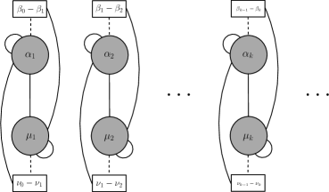
Figure 1: A generic one dimensional quiver field theory whose IR limit is dual to the AdS₂ backgrounds given in [1].

The proposal in [1] is that the one dimensional $\mathcal{N}=4$ quantum mechanics living on the complete D0-D4-D$4^{\prime}$-D8-F1 brane intersection describes the interactions between the two types of instantons and two types of Wilson loops in the $Q_{\text{D}4^{\prime}}^{m}\times Q_{\text{D}8}^{m}$ antisymmetric representation of $\text{U}(Q_{\text{D}4}^{e})\times\text{U}(Q_{\text{D}0}^{e})$.

The SCQMs that live on these brane set-ups were analysed in [1]. They are described in terms of a set of disconnected quivers as shown in Figure 1, with gauge groups associated to the colour D0 and D4 branes (the latter wrapped on the CY₂) coupled to the D$4^{\prime}$ and D8 flavour branes. The dynamics is described in terms of (4,4) vector multiplets, associated to gauge nodes (circles); (4,4) hypermultiplets in the adjoint representation connecting one gauge node to itself (semicircles in black lines); and (4,4) hypermultiplets in the bifundamental representation of the two gauge groups (vertical black lines). The connection with the flavour groups is through twisted (4,4) bifundamental hypermultiplets, connecting the D0-branes with the D$4^{\prime}$-branes and the D4-branes with the D8-branes (bent black lines), and (0,2) bifundamental Fermi multiplets, connecting the D4-branes with the D$4^{\prime}$-branes and the D0-branes with the D8-branes (dashed lines) –see [1] for more details.

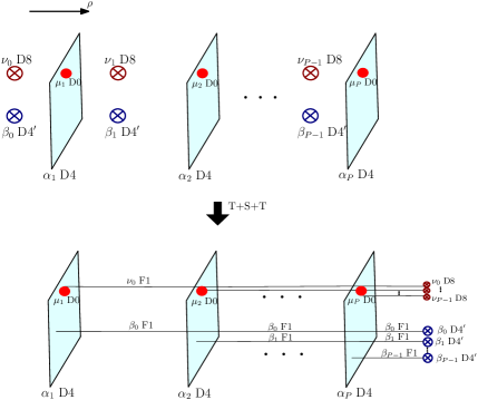
Figure 2: (Top) Hanany-Witten like brane set-up associated with the quivers depicted in Figure 1. Brane set-up equivalent to the previous one after a T+S+T duality transformation and Hanany-Witten moves (bottom).

Such quivers, depicted in Figure 1, can be read from the Hanany-Witten like brane set-up depicted at the top of Figure 2. Here in each $[\rho_{k},\rho_{k+1}]$ interval there are $\mu_{k}$ D0-branes and $\alpha_{k}$ D4-branes, playing the rôle of colour branes. Orthogonal to them there are $\nu_{k}$ D8-branes and $\beta_{k}$ D$4^{\prime}$-branes, interpreted as flavour branes. In order to see the interpretation as Wilson lines one can proceed as follows (see [1]). The D0-D4-D$4^{\prime}$-D8-F1 brane set-up is taken to an F1-D3-NS5-NS7-D1 system in Type IIB through a T+S duality transformation. In this set-up, Hanany-Witten moves can be performed, which upon T-duality give the Type IIA configuration depicted at the bottom of Figure 2. This configuration consists of $\nu_{k}$ coincident stacks of D8-branes and $\beta_{k}$ coincident stacks of D$4^{\prime}$-branes, with $\mu_{k}$ and $\alpha_{k}$ F1-strings originating in the different $(\nu_{0},\nu_{1},...\nu_{k-1};\beta_{0},\beta_{1},...,\beta_{k-1})$ coincident stacks of D8- and D$4^{\prime}$-branes. The other endpoint of the F1-strings is on each stack of $\mu_{k}$ D0-branes and $\alpha_{k}$ D4-branes. From this picture the description of Wilson loops in the $(\nu_{0},\nu_{1},...\nu_{k-1};\beta_{0},\beta_{1},...,\beta_{k-1})$ completely antisymmetric representation of U$(\mu_{k})$ and U$(\alpha_{k})$, respectively, is recovered. In [1], this was interpreted as describing Wilson lines for each of the D0 and D4 gauge groups, given that they are in the completely antisymmetric representation they actually described backreacted D4-D0 baryon vertices [82] within the 5d CFT living in D4^′-D8 brane intersections. The reader is referred to [1] for more details on this construction.

In [1], it was shown that the holographic central charge (given by (3.15)), matches the field theory central charge, computed using the expression,

$$c_{ft}=6(n_{hyp}-n_{vec}),$$ (3.16)

where $n_{hyp}$ counts the number of bifundamental, fundamental and adjoint (0,4) hypermultiplets and $n_{vec}$ counts the number of (0,4) vector multiplets, both in the UV description. The equation (3.16) was obtained in [83] for two-dimensional conformal field theories, and was determined by identifying the right-handed central charge with the U$(1)_{R}$ current two-point function. With the expression (3.16), both results, holographic and field theory central charge have been shown to agree for the 2d $\mathcal{N}=(0,4)$ quiver CFTs constructed in [27, 28, 29], as well as for the AdS₂/SCQM pairs proposed in [1, 38, 41]. In [38], the agreement is kept since the one-dimensional quiver QMs are originated from the two-dimensional $\mathcal{N}=(0,4)$ CFTs upon dimensional reduction. However, in [1, 41], the equation (3.16) matches with the holographic result even though the 1d CFTs have not originated from the 2d “mother” CFTs.

As we anticipated, the background (2.17) belongs to the classification provided in [1]. Therefore, we will use the expression (3.16) to obtain the number of vacua of the superconformal quantum mechanics dual to our solution. The previous analysis guarantees its agreement with the holographic result.

After this summary, we turn to the solution (2.17), the main focus of this paper and show that it fits locally in the previous class of AdS${}_{2}\times$S${}^{3}\times$CY${}_{2}\times$I solutions to Type IIA supergravity constructed in [1].

4 SCQM dual to the non-Abelian T-dual solution

In this section we show that the solution (2.17), obtained as the SL($2,\mathbf{R}$)-NATD of the AdS${}_{3}\times$S${}^{3}\times$CY₂ solution to Type IIB supergravity, fits in the class of geometries constructed in [1], that we have just reviewed. We will also provide a global completion to this solution by glueing it to itself.

Consider the backgrounds (3.1). It is easy to see that the background (2.17) fits locally in this class of solutions, with the simple choices,

$$\begin{split}u=4L^{4}M^{2}\rho,\qquad h_{4}=L^{2}M^{4}\rho,\qquad h_{8}=F_{0}\rho\,.\end{split}$$ (4.1)

In [29], it was studied that the AdS${}_{3}\times$S${}^{2}\times$CY${}_{2}\times$I solution constructed in [56], by acting SU(2)-NATD on the near horizon limit of the D1-D5 system, belongs to a subset of the geometries classified in [26]. Therefore, since both classifications, [26] and [34, 1], are related by a double analytical continuation, this fact strongly suggests that the background (2.17) should be related to the solution obtained in [56], upon an analytical continuation prescription.

This double analytical continuation works as follows, we focus on the Type IIA background given by (2.17) and the AdS₂ and S₃ factors are interchanged as,

$$\begin{split}&\text{d}s_{\text{AdS}_{2}}^{2}\to-\text{d}s_{\text{S}^{2}}^{2},\qquad\text{d}s_{\text{S}^{3}}^{2}\to-\text{d}s_{\text{AdS}_{3}}^{2}.\end{split}$$ (4.2)

In order to get well-defined supergravity fields, we also need to analytically continue the following terms,

$$\begin{split}\rho\to i\rho,\qquad L\to iL,\qquad F_{i}\to-F_{i},\end{split}$$ (4.3)

where $F_{i}$ are the RR fluxes. Thus, applying this set of transformations one finds the AdS${}_{3}\times$S${}^{2}\times$ CY${}_{2}\times$I solution to massive Type IIA supergravity with four Poincaré supersymmetries constructed for the first time in [56]. We summarise these connexions in Figure 3.

Figure 3: Relation between the solution (2.17) and the solution obtained in [56] through SU(2)-NATD.

4.1 Completed NATD solution

According to (3.6)-(3.10) one can choose a profile for the piecewise linear functions $h_{4}$, $h_{8}$ and propose a concrete way to complete the solution (2.17). In turn, completing the geometry implies a completion in the quiver, allowing us to match between holographic and field theory computations.

We can complete the solution (2.17) by terminating the $\rho$ interval at a certain value $\rho_{2P}$ with $P\in\mathbb{Z}$. Then, the piecewise functions (3.6)-(3.10) read,

$$u=4L^{4}M^{2}\rho,$$ (4.4)

$$h_{4}(\rho)\!=\!\!L^{2}M^{4}\;\!\!\left\{\begin{array}[]{cccrcl}\rho&\rho_{0}\leq\rho\leq\rho_{P}\;,&\\ \rho_{0}-(\rho-\rho_{2P})&~{}~{}\rho_{P}\leq\rho\leq\rho_{2P},&\end{array}\right.$$ (4.7)

$$h_{8}(\rho)=\!\!L^{2}\;\!\!\left\{\begin{array}[]{cccrcl}\rho&\rho_{0}\leq\rho\leq{\rho_{P}},&\\ {\rho_{0}}-(\rho-\rho_{2P})&~{}~{}{\rho_{P}}\leq\rho\leq\rho_{2P}.&\end{array}\right.$$ (4.10)

The previous functions reproduce the behaviour (2.19) for the metric and dilaton at both ends of the space and one can check that the NS sector is continuous at $\rho_{P}$ when $\rho_{P}=\frac{\rho_{0}+\rho_{2P}}{2}$. Hereinafter, we take the value $\rho_{2P}=\rho_{0}\;(2P-1)$ and use $\frac{\rho_{0}}{2\pi}$ dimensionless, namely $\frac{\rho_{0}}{2\pi}\to 1$, in order to obtain well-quantised charges. Thus, we get $\rho_{P}=2\pi P$.

Notice that the functions (4.7)-(4.10) are a simple example, with $\beta_{k}=\beta$ and $\nu_{k}=\nu$, for all intervals. This implies there are no flavour branes at the different intervals –with the exception of the [$\rho_{P-1},\rho_{P}$] interval, that we will analyse later.

The Page fluxes (2.23) in each $[\rho_{k},\rho_{k+1}]$ interval then read as follows,

$$\hat{F}_{0} \!=\!\!L^{2}\;\!\!\left\{\begin{array}[]{cccrcl}1&k=0,...,P-1,&\\ -1&~{}~{}~{}~{}k=P,...,(2P-1),&\end{array}\right.$$ (4.13)

$$\hat{F}_{2} =\!\!\pi L^{2}\text{vol}_{\text{AdS}_{2}}\;\!\!\left\{\begin{array}[]{cccrcl}-k&k=0,...,P-1,&\\ -(2P-k)&~{}~{}~{}~{}k=P,...,(2P-1),&\end{array}\right.$$ (4.16)

$$\hat{F}_{4}^{\text{CY}_{2}} =\!\!L^{2}M^{4}\text{vol}_{\text{CY}_{2}}\;\!\!\left\{\begin{array}[]{cccrcl}-1&~{}~{}~{}~{}k=0,...,P-1,&\\ 1&~{}~{}~{}~{}~{}~{}~{}~{}k=P,...,(2P-1),&\end{array}\right.$$ (4.19)

$$\hat{F}_{6}^{\text{CY}_{2}} =\!\!\pi L^{2}M^{4}\text{vol}_{\text{AdS}_{2}}\wedge\text{vol}_{\text{CY}_{2}}\;\!\!\left\{\begin{array}[]{cccrcl}k&k=0,...,P-1,&\\ (2P-k)&~{}~{}~{}~{}k=P,...,(2P-1),&\end{array}\right.$$ (4.22)

Here we show the component over CY₂ for $\hat{F}_{4}$ and $\hat{F}_{6}$. The 2-form and 6-form Page fluxes are continuous at $\rho_{P}$ and the change of sign in the 0-form and 4-form Page fluxes is due to the presence of D8 and D$4^{\prime}$ flavour branes at [$\rho_{P-1},\rho_{P}$] interval.

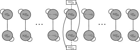
Figure 4: Symmetric completed quiver associated to the NATD solution.

The corresponding quantised charges read,

$$Q_{\text{D8}}^{m}\! =\!\!2\pi L^{2}\;\!\!\left\{\begin{array}[]{cccrcl}1&k=0,...,P-1,&\\ -1&~{}~{}~{}~{}k=P,...,(2P-1),&\end{array}\right.$$ (4.25)

$$Q_{\text{D0}}^{e} =\!\!Q_{\text{D8}}^{m}\;\!\!\left\{\begin{array}[]{cccrcl}-k&k=0,...,P-1,&\\ -(2P-k)&~{}~{}~{}~{}k=P,...,(2P-1),&\end{array}\right.$$ (4.28)

$$Q_{\text{D4}^{\prime}}^{m} =\!\!2\pi L^{2}M^{4}\;\!\!\left\{\begin{array}[]{cccrcl}-1&k=0,...,P-1,&\\ 1&~{}~{}~{}~{}k={P},...,(2P-1),&\end{array}\right.$$ (4.31)

$$Q_{\text{D4}}^{e} =\!\!Q_{\text{D$4^{\prime}$}}^{m}\;\!\!\left\{\begin{array}[]{cccrcl}k&k=0,...,P-1,&\\ (2P-k)&~{}~{}~{}~{}k=P,...,(2P-1).&\end{array}\right.$$ (4.34)

Thus, the D0 and D4 brane charges increase linearly in the $0\leq k\leq P$ region, and decrease linearly in the $P+1\leq k\leq 2P-1$ region, until the value $k=2P-1$ is reached. Here the minus sign in the charges denotes anti-Dp brane charge. The quiver for the configuration (4.7)-(4.10) is depicted in Figure 4.

The discontinuities at $\rho_{P}$ are translated into $2Q_{\text{D$4^{\prime}$}}^{m}$ and $2Q_{\text{D8}}^{m}$ flavour groups according to,

$$N_{\text{D4}^{\prime}}^{\left[P-1,P\right]} = \frac{1}{(2\pi)^{3}}\int_{\text{CY}_{2}}\hat{F}_{4}=\frac{1}{(2\pi)^{3}}\int_{\text{CY}_{2}\times\text{I}_{\rho}}\text{d}\hat{F}_{4}=\beta_{P-1}-\beta_{P}=2Q_{\text{D$4^{\prime}$}}^{m}$$ (4.35)

$$N_{\text{D8}}^{\left[P-1,P\right]} = 2\pi\hat{F}_{0}=2\pi\int_{\text{I}_{\rho}}\text{d}\hat{F}_{0}=\nu_{P-1}-\nu_{P}=2Q_{\text{D8}}^{m}$$ (4.36)

where we used the expressions (3.13)-(3.14) with $\beta_{P-1}=2\pi L^{2}M^{4}$, $\beta_{P}=-2\pi L^{2}M^{4}$, $\nu_{P-1}=2\pi L^{2}$ and $\nu_{P}=-2\pi L^{2}$.

The quiver shown in Figure 4 can be translated to the description reviewed in Section 3.1. The Hanany-Witten like brane set-up is shown in Figure 5. In each $[\rho_{k},\rho_{k+1}]$ interval, for $k=0,...,P-1$, we have $kQ_{\textrm{D8}}^{m}$ D0-branes and $kQ_{\textrm{D4}^{\prime}}^{m}$ D4-branes. For $k=P,...,2P-1$ we have $(2P-k)Q_{\textrm{D8}}^{m}$ D0-branes and $(2P-k)Q_{\textrm{D4}^{\prime}}^{m}$ D4-branes. Orthogonal to them, in each interval, there are $Q_{\textrm{D8}}^{m}$ D8-branes and $Q_{\textrm{D4}^{\prime}}^{m}$ D4^′-branes, playing the rôle of flavour branes.

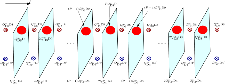
Figure 5: The Hanany-Witten like brane set-up for the completed non-Abelian T-dual solution, underlying the quiver depicted in Figure 4.

As proposed in [1] and we reviewed in Section 3.1, one can perform a T-S-T duality transformation to the D0-D4-D4^′-D8-F1 system. Consider the left-hand side of the Hanany-Witten like brane set-up shown in Figure 5, from the first $Q_{\textrm{D8}}^{m}\text{D}8$- and $Q_{\textrm{D4}^{\prime}}^{m}\text{D}4^{\prime}$-branes until the $PQ_{\textrm{D8}}^{m}\text{D}0$- and $PQ_{\textrm{D4}^{\prime}}^{m}\text{D}4$-branes. It is easy to see that this subsystem is equivalent to the brane set-up depicted on the top of Figure 2 (with $\nu_{i}=Q_{\textrm{D8}}^{m}$, $\beta_{i}=Q_{\textrm{D4}^{\prime}}^{m}$, $\mu_{j}=jQ_{\textrm{D8}}^{m}$ and $\alpha_{j}=jQ_{\textrm{D4}^{\prime}}^{m}$, for $i=0,1,...,P-1$ and $j=1,...,P$). When we perform the T+S+T transformation on the left-hand configuration an equivalent system to the bottom in Figure 2 is obtained. This is depicted on the left-hand side in Figure 6, here the now coincident D8-branes and D4^′-branes are to the right of the $PQ_{\textrm{D8}}^{m}$D0 and $PQ_{\textrm{D4}^{\prime}}^{m}$D4 stacks. On the right-hand side of the Hanany-Witten like brane set-ups, shown in Figure 5 and Figure 6, we have the same configuration that on the left-hand side, since the right-hand side is the symmetric part of the left-hand side. That is, the complete configuration is the left-hand side glued to itself.

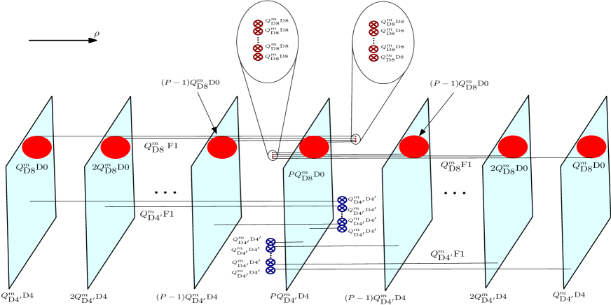
Figure 6: Symmetric brane set-up after a T+S+T duality transformation and Hanany-Witten moves from the brane set-up depicted in Figure 5.

Let us focus on the D0-D8-F1 system on the left-hand side of the Hanany-Witten like brane set-up shown in Figure 6 (from $Q_{\textrm{D8}}^{m}\text{D}0$ until $PQ_{\textrm{D8}}^{m}\text{D}0$). After the T+S+T transformation, we obtain $P$ stacks of $Q_{\textrm{D8}}^{m}$D8-branes –depicted in Figure 6 to the right of the $PQ_{\textrm{D8}}^{m}$D0-branes– with $PQ_{\textrm{D8}}^{m}$F1-strings originating in the different coincident stacks of D8-branes. The other endpoint of the F1-strings is on each stack of $kQ_{\textrm{D8}}^{m}$D0-branes. For the D4-D4^′-F1 system we have a similar configuration, namely $P$ stacks of $Q_{\textrm{D4}^{\prime}}^{m}$D4^′-branes, with $PQ_{\textrm{D4}^{\prime}}^{m}$F1-strings attached to them. These F1-strings have the other end point on the different $kQ_{\textrm{D4}^{\prime}}^{m}$ stacks of D4-branes. Thus, as we reviewed in Section 3.1, the system can be interpreted as Wilson loops in the $Q_{\textrm{D8}}^{m}\times Q_{\textrm{D4}^{\prime}}^{m}$ completely antisymmetric representation of the gauge groups U$(kQ_{\textrm{D8}}^{m})\times$U$(kQ_{\textrm{D4}^{\prime}}^{m})$, that we interpret as describing the backreaction of the D4-D0 baryon vertices of a D4^′-D8 brane intersection.

To be concrete, consider the SCQM that arises in the very low energy limit of a D4^′-D8 brane intersection, dual to a 5d QFT, where D4- and D0-brane baryon vertices are introduced. Namely, D4-brane (D0-brane) baryon vertices are linked to D4^′-branes (D8-branes) with fundamental strings. In the IR these branes change their rôle, that is the gauge symmetry on both D4^′- and D8-branes becomes global, shifting D4^′ and D8 from colour to flavour branes and the D0- and D4-branes play now the rôle of colour branes of the backreacted geometry.

Furthermore, with the piecewise linear functions (4.4), (4.7) and (4.10) we can compute the holographic central charge,

$$\begin{split}c_{hol}&=\frac{3}{\pi}L^{4}M^{4}\left(\int_{\rho_{0}}^{\rho_{P}}(\rho^{2}-\rho_{0}^{2})\;\text{d}\rho+\int_{\rho_{P}}^{\rho_{2P}}\left(\left(\rho_{0}-(\rho-\rho_{2P})\right)^{2}-\rho_{0}^{2}\right)\;\text{d}\rho\right)\\ &=Q_{\text{D4}^{\prime}}^{m}Q_{\text{D8}}^{m}(4P^{3}-12P+8).\end{split}$$ (4.37)

In order to compare this result with the field theory computation in (3.16), we need to compute the number of hypermultiplets and vector multiplets. For the quiver in Figure 4 we obtain,

$$\begin{split}n_{hyp}&=\left((Q_{\text{D$4^{\prime}$}}^{m})^{2}+(Q_{\text{D8}}^{m})^{2}+Q_{\text{D4}^{\prime}}^{m}Q_{\text{D8}}^{m}\right)\left(P^{2}+2\sum_{i=1}^{P-1}i^{2}\right),\\ n_{vec}&=\left((Q_{\text{D$4^{\prime}$}}^{m})^{2}+(Q_{\text{D8}}^{m})^{2}\right)\left(P^{2}+2\sum_{i=1}^{P-1}i^{2}\right).\end{split}$$ (4.38)

Thus, when the sums are performed we get the following expression for the field theory central charge,

$$\begin{split}c_{ft}=6(n_{hyp}-n_{vec})&=6Q_{\text{D4}^{\prime}}^{m}Q_{\text{D8}}^{m}\left(P^{2}+2\sum_{i=1}^{P-1}i^{2}\right)\\ &=Q_{\text{D4}^{\prime}}^{m}Q_{\text{D8}}^{m}(4P^{3}+2P).\end{split}$$ (4.39)

We see that at large $Q_{\text{D8}}^{m}$, $Q_{\text{D4}^{\prime}}^{m}$ and $P$ (in the holographic limit, which is long quivers with large ranks) the results (4.37) and (4.39) coincide.

5 Conclusions

In this paper we developed the implementation of NATD in supergravity backgrounds supporting an SL(2,$\mathbf{R}$) subgroup as part of their full isometry group. Namely, we implemented the solution generating technique in non-compact spaces exhibiting an SO(2,2) $\cong$ SL(2,$\mathbf{R})_{L}\times$SL(2,$\mathbf{R})_{R}$ isometry group geometrically realised by an AdS₃ space. After the dualisation, the resultant dual geometry exhibits an SL(2,$\mathbf{R}$) isometry reflected geometrically as an AdS₂ space plus a non-compact new direction in the internal space. This non-compact direction arises since the Lagrange multipliers live in the Lie algebra of the SL(2,$\mathbf{R}$) group, which is by construction a vector space, $\mathbf{R}^{3}$. That is, the space dual to AdS₃ is locally AdS${}_{2}\times\mathbf{R}^{+}$.

We worked out in detail the SL(2,$\mathbf{R}$)-NATD solution of the AdS${}_{3}\times$S${}^{3}\times$CY₂ solution that arises in the near horizon limit of the D1-D5 brane intersection. We found that the SL(2,$\mathbf{R}$)-NATD solution is a simple example in the classification constructed in [1]. Further, our background (2.17) is related through an analytic continuation prescription to the AdS${}_{3}\times$S${}^{2}\times$CY${}_{2}\times$I solution obtained in [56], as one of the first examples of AdS backgrounds generated through SU(2) non-Abelian T-duality.

An important drawback of non-Abelian T-duality is the lack of global information about the dual geometry, which cannot be inferred from the transformation itself. For this we used the fact that our solution (2.17) fits in the classification constructed in [1] which allowed us to propose an explicit completion for the geometry. Unlike the two completions worked out in [29] for the SU(2)-NATD solution constructed therein, continuity of the NS sector allows only one possible completion for the geometry given in (2.17). Our completion, shown in Section 4.1, is obtained by glueing the SL(2,$\mathbf{R}$)-NATD solution to itself. We proposed a well-defined quiver quantum mechanics, dual to our AdS₂ solution, that flows in the IR to a superconformal quantum mechanics (based on the Hanany-Witten brane set-ups and Page charges), which admits an interpretation in terms of backreacted D4-D0 baryon vertices within the 5d QFT living in a D4^′-D8 brane intersection. In support of our proposal we checked the agreement between the holographic and field theory central charges.

References

- [1] Y. Lozano, C. Nunez, A. Ramirez, and S. Speziali, “AdS2 duals to ADHM quivers with Wilson lines,” JHEP 03 (2021) 145, arXiv:2011.13932 [hep-th].
- [2] F. Benini, K. Hristov, and A. Zaffaroni, “Black hole microstates in AdS4 from supersymmetric localization,” JHEP 05 (2016) 054, arXiv:1511.04085 [hep-th].
- [3] F. Benini, K. Hristov, and A. Zaffaroni, “Exact microstate counting for dyonic black holes in AdS4,” Phys. Lett. B 771 (2017) 462–466, arXiv:1608.07294 [hep-th].
- [4] A. Cabo-Bizet, V. I. Giraldo-Rivera, and L. A. Pando Zayas, “Microstate counting of AdS4 hyperbolic black hole entropy via the topologically twisted index,” JHEP 08 (2017) 023, arXiv:1701.07893 [hep-th].
- [5] J. M. Maldacena, “The Large N limit of superconformal field theories and supergravity,” Int. J. Theor. Phys. 38 (1999) 1113–1133, arXiv:hep-th/9711200 [hep-th]. [Adv. Theor. Math. Phys.2,231(1998)].
- [6] J. M. Maldacena, J. Michelson, and A. Strominger, “Anti-de Sitter fragmentation,” JHEP 02 (1999) 011, arXiv:hep-th/9812073.
- [7] F. Denef, D. Gaiotto, A. Strominger, D. Van den Bleeken, and X. Yin, “Black Hole Deconstruction,” JHEP 03 (2012) 071, arXiv:hep-th/0703252.
- [8] J. Maldacena and D. Stanford, “Remarks on the Sachdev-Ye-Kitaev model,” Phys. Rev. D 94 no. 10, (2016) 106002, arXiv:1604.07818 [hep-th].
- [9] J. Maldacena, D. Stanford, and Z. Yang, “Conformal symmetry and its breaking in two dimensional Nearly Anti-de-Sitter space,” PTEP 2016 no. 12, (2016) 12C104, arXiv:1606.01857 [hep-th].
- [10] D. Harlow and D. Jafferis, “The Factorization Problem in Jackiw-Teitelboim Gravity,” JHEP 02 (2020) 177, arXiv:1804.01081 [hep-th].
- [11] M. Cvetic, H. Lu, C. Pope, and J. F. Vazquez-Poritz, “AdS in warped space-times,” Phys. Rev. D 62 (2000) 122003, arXiv:hep-th/0005246.
- [12] J. P. Gauntlett, N. Kim, and D. Waldram, “Supersymmetric AdS(3), AdS(2) and Bubble Solutions,” JHEP 04 (2007) 005, arXiv:hep-th/0612253.
- [13] E. D’Hoker, J. Estes, and M. Gutperle, “Gravity duals of half-BPS Wilson loops,” JHEP 06 (2007) 063, arXiv:0705.1004 [hep-th].
- [14] M. Chiodaroli, M. Gutperle, and D. Krym, “Half-BPS Solutions locally asymptotic to AdS(3) x S**3 and interface conformal field theories,” JHEP 02 (2010) 066, arXiv:0910.0466 [hep-th].
- [15] M. Chiodaroli, E. D’Hoker, and M. Gutperle, “Open Worldsheets for Holographic Interfaces,” JHEP 03 (2010) 060, arXiv:0912.4679 [hep-th].
- [16] N. Kim, “Comments on solutions from M2-branes on complex curves and the backreacted Kähler geometry,” Eur. Phys. J. C 74 no. 2, (2014) 2778, arXiv:1311.7372 [hep-th].
- [17] O. Kelekci, Y. Lozano, J. Montero, E. Colgáin, and M. Park, “Large superconformal near-horizons from M-theory,” Phys. Rev. D 93 no. 8, (2016) 086010, arXiv:1602.02802 [hep-th].
- [18] C. Couzens, C. Lawrie, D. Martelli, S. Schafer-Nameki, and J.-M. Wong, “F-theory and AdS3/CFT2,” JHEP 08 (2017) 043, arXiv:1705.04679 [hep-th].
- [19] G. Dibitetto and N. Petri, “6d surface defects from massive type IIA,” JHEP 01 (2018) 039, arXiv:1707.06154 [hep-th].
- [20] D. Corbino, E. D’Hoker, and C. F. Uhlemann, “AdS S6 versus AdS S2 in Type IIB supergravity,” JHEP 03 (2018) 120, arXiv:1712.04463 [hep-th].
- [21] G. Dibitetto and N. Petri, “Surface defects in the D4 D8 brane system,” JHEP 01 (2019) 193, arXiv:1807.07768 [hep-th].
- [22] G. Dibitetto and N. Petri, “AdS2 solutions and their massive IIA origin,” JHEP 05 (2019) 107, arXiv:1811.11572 [hep-th].
- [23] D. Corbino, E. D’Hoker, J. Kaidi, and C. F. Uhlemann, “Global half-BPS solutions in Type IIB,” JHEP 03 (2019) 039, arXiv:1812.10206 [hep-th].
- [24] N. T. Macpherson, “Type II solutions on AdS S S3 with large superconformal symmetry,” JHEP 05 (2019) 089, arXiv:1812.10172 [hep-th].
- [25] J. Hong, N. T. Macpherson, and L. A. Pando Zayas, “Aspects of AdS2 classification in M-theory: solutions with mesonic and baryonic charges,” JHEP 11 (2019) 127, arXiv:1908.08518 [hep-th].
- [26] Y. Lozano, N. T. Macpherson, C. Nunez, and A. Ramirez, “AdS3 solutions in Massive IIA with small supersymmetry,” arXiv:1908.09851 [hep-th].
- [27] Y. Lozano, N. T. Macpherson, C. Nunez, and A. Ramirez, “1/4 BPS solutions and the AdS3/CFT2 correspondence,” Phys. Rev. D 101 no. 2, (2020) 026014, arXiv:1909.09636 [hep-th].
- [28] Y. Lozano, N. T. Macpherson, C. Nunez, and A. Ramirez, “Two dimensional quivers dual to AdS3 solutions in massive IIA,” JHEP 01 (2020) 140, arXiv:1909.10510 [hep-th].
- [29] Y. Lozano, N. T. Macpherson, C. Nunez, and A. Ramirez, “AdS3 solutions in massive IIA, defect CFTs and T-duality,” JHEP 12 (2019) 013, arXiv:1909.11669 [hep-th].
- [30] A. Legramandi and N. T. Macpherson, “AdS3 solutions with from from SS3 fibrations,” Fortsch. Phys. 68 no. 3-4, (2020) 2000014, arXiv:1912.10509 [hep-th].
- [31] G. Dibitetto, Y. Lozano, N. Petri, and A. Ramirez, “Holographic description of M-branes via AdS2,” JHEP 04 (2020) 037, arXiv:1912.09932 [hep-th].
- [32] D. Lüst and D. Tsimpis, “AdS2 type-IIA solutions and scale separation,” JHEP 07 (2020) 060, arXiv:2004.07582 [hep-th].
- [33] D. Corbino, “Warped and symmetry in Type IIB,” arXiv:2004.12613 [hep-th].
- [34] Y. Lozano, C. Nunez, A. Ramirez, and S. Speziali, “-strings and AdS3 solutions to M-theory with small supersymmetry,” JHEP 08 (2020) 118, arXiv:2005.06561 [hep-th].
- [35] K. Chen, M. Gutperle, and M. Vicino, “Holographic Line Defects in , Gauged Supergravity,” Phys. Rev. D 102 no. 2, (2020) 026025, arXiv:2005.03046 [hep-th].
- [36] F. Faedo, Y. Lozano, and N. Petri, “New AdS3 near-horizons in Type IIB,” arXiv:2012.07148 [hep-th].
- [37] F. Faedo, Y. Lozano, and N. Petri, “Searching for surface defect CFTs within AdS3,” arXiv:2007.16167 [hep-th].
- [38] Y. Lozano, C. Nunez, A. Ramirez, and S. Speziali, “New AdS2 backgrounds and Conformal Quantum Mechanics,” JHEP 03 (2021) 277, arXiv:2011.00005 [hep-th].
- [39] A. Passias and D. Prins, “On supersymmetric AdS3 solutions of Type II,” arXiv:2011.00008 [hep-th].
- [40] A. Legramandi, G. Lo Monaco, and N. T. Macpherson, “All AdS3 solutions in 10 and 11 dimensions,” JHEP 05 (2021) 263, arXiv:2012.10507 [hep-th].
- [41] Y. Lozano, C. Nunez, and A. Ramirez, “ solutions in Type IIB with 8 supersymmetries,” JHEP 04 (2021) 110, arXiv:2101.04682 [hep-th].
- [42] J. R. Balaguer, G. Dibitetto, and J. J. Fernández-Melgarejo, “New IIB intersecting brane solutions yielding supersymmetric AdS3 vacua,” arXiv:2104.03970 [hep-th].
- [43] S. Zacarias, “Marginal deformations of a class of AdS3 holographic backgrounds,” arXiv:2102.05681 [hep-th].
- [44] D. Roychowdhury, “Fragmentation and defragmentation of strings in type IIA and their holographic duals,” arXiv:2104.11953 [hep-th].
- [45] X. C. de la Ossa and F. Quevedo, “Duality symmetries from nonAbelian isometries in string theory,” Nucl. Phys. B 403 (1993) 377–394, arXiv:hep-th/9210021.
- [46] M. Rocek and E. P. Verlinde, “Duality, quotients, and currents,” Nucl. Phys. B 373 (1992) 630–646, arXiv:hep-th/9110053.
- [47] A. Giveon and M. Rocek, “On nonAbelian duality,” Nucl. Phys. B 421 (1994) 173–190, arXiv:hep-th/9308154.
- [48] E. Alvarez, L. Alvarez-Gaume, and Y. Lozano, “On nonAbelian duality,” Nucl. Phys. B 424 (1994) 155–183, arXiv:hep-th/9403155.
- [49] K. Sfetsos, “Gauged WZW models and nonAbelian duality,” Phys. Rev. D 50 (1994) 2784–2798, arXiv:hep-th/9402031.
- [50] Y. Lozano, “NonAbelian duality and canonical transformations,” Phys. Lett. B 355 (1995) 165–170, arXiv:hep-th/9503045.
- [51] K. Sfetsos, “NonAbelian duality, parafermions and supersymmetry,” Phys. Rev. D 54 (1996) 1682–1695, arXiv:hep-th/9602179.
- [52] E. Alvarez, L. Alvarez-Gaume, J. Barbon, and Y. Lozano, “Some global aspects of duality in string theory,” Nucl. Phys. B 415 (1994) 71–100, arXiv:hep-th/9309039.
- [53] E. Alvarez, L. Alvarez-Gaume, and Y. Lozano, “A Canonical approach to duality transformations,” Phys. Lett. B 336 (1994) 183–189, arXiv:hep-th/9406206.
- [54] S. Elitzur, A. Giveon, E. Rabinovici, A. Schwimmer, and G. Veneziano, “Remarks on nonAbelian duality,” Nucl. Phys. B 435 (1995) 147–171, arXiv:hep-th/9409011.
- [55] C. Klimcik and P. Severa, “Dual nonAbelian duality and the Drinfeld double,” Phys. Lett. B 351 (1995) 455–462, arXiv:hep-th/9502122.
- [56] K. Sfetsos and D. C. Thompson, “On non-abelian T-dual geometries with Ramond fluxes,” Nucl. Phys. B 846 (2011) 21–42, arXiv:1012.1320 [hep-th].
- [57] Y. Lozano, E. O Colgain, K. Sfetsos, and D. C. Thompson, “Non-abelian T-duality, Ramond Fields and Coset Geometries,” JHEP 06 (2011) 106, arXiv:1104.5196 [hep-th].
- [58] Y. Lozano, E. Ó Colgáin, D. Rodríguez-Gómez, and K. Sfetsos, “Supersymmetric via T Duality,” Phys. Rev. Lett. 110 no. 23, (2013) 231601, arXiv:1212.1043 [hep-th].
- [59] G. Itsios, C. Nunez, K. Sfetsos, and D. C. Thompson, “On Non-Abelian T-Duality and new N=1 backgrounds,” Phys. Lett. B 721 (2013) 342–346, arXiv:1212.4840 [hep-th].
- [60] G. Itsios, Y. Lozano, E. O Colgain, and K. Sfetsos, “Non-Abelian T-duality and consistent truncations in type-II supergravity,” JHEP 08 (2012) 132, arXiv:1205.2274 [hep-th].
- [61] G. Itsios, C. Nunez, K. Sfetsos, and D. C. Thompson, “Non-Abelian T-duality and the AdS/CFT correspondence:new N=1 backgrounds,” Nucl. Phys. B 873 (2013) 1–64, arXiv:1301.6755 [hep-th].
- [62] A. Barranco, J. Gaillard, N. T. Macpherson, C. Núñez, and D. C. Thompson, “G-structures and Flavouring non-Abelian T-duality,” JHEP 08 (2013) 018, arXiv:1305.7229 [hep-th].
- [63] N. T. Macpherson, “Non-Abelian T-duality, -structure rotation and holographic duals of Chern-Simons theories,” JHEP 11 (2013) 137, arXiv:1310.1609 [hep-th].
- [64] Y. Lozano, E. Ó Colgáin, and D. Rodríguez-Gómez, “Hints of 5d Fixed Point Theories from Non-Abelian T-duality,” JHEP 05 (2014) 009, arXiv:1311.4842 [hep-th].
- [65] S. Zacarías, “Semiclassical strings and Non-Abelian T-duality,” Phys. Lett. B 737 (2014) 90–97, arXiv:1401.7618 [hep-th].
- [66] Y. Lozano and N. T. Macpherson, “A new AdS4/CFT3 dual with extended SUSY and a spectral flow,” JHEP 11 (2014) 115, arXiv:1408.0912 [hep-th].
- [67] K. Sfetsos and D. C. Thompson, “New supersymmetric backgrounds in Type IIA supergravity,” JHEP 11 (2014) 006, arXiv:1408.6545 [hep-th].
- [68] O. Kelekci, Y. Lozano, N. T. Macpherson, and E. O. Colgáin, “Supersymmetry and non-Abelian T-duality in type II supergravity,” Class. Quant. Grav. 32 no. 3, (2015) 035014, arXiv:1409.7406 [hep-th].
- [69] N. T. Macpherson, C. Núñez, L. A. Pando Zayas, V. G. J. Rodgers, and C. A. Whiting, “Type IIB supergravity solutions with AdS5 from Abelian and non-Abelian T dualities,” JHEP 02 (2015) 040, arXiv:1410.2650 [hep-th].
- [70] K. S. Kooner and S. Zacarías, “Non-Abelian T-Dualizing the Resolved Conifold with Regular and Fractional D3-Branes,” JHEP 08 (2015) 143, arXiv:1411.7433 [hep-th].
- [71] Y. Lozano, N. T. Macpherson, and J. Montero, “A supersymmetric AdS4 solution in M-theory with purely magnetic flux,” JHEP 10 (2015) 004, arXiv:1507.02660 [hep-th].
- [72] N. T. Macpherson, C. Nunez, D. C. Thompson, and S. Zacarias, “Holographic Flows in non-Abelian T-dual Geometries,” JHEP 11 (2015) 212, arXiv:1509.04286 [hep-th].
- [73] J. van Gorsel and S. Zacarías, “A Type IIB Matrix Model via non-Abelian T-dualities,” JHEP 12 (2017) 101, arXiv:1711.03419 [hep-th].
- [74] Y. Lozano and C. Núñez, “Field theory aspects of non-Abelian T-duality and 2 linear quivers,” JHEP 05 (2016) 107, arXiv:1603.04440 [hep-th].
- [75] Y. Lozano, N. T. Macpherson, J. Montero, and C. Nunez, “Three-dimensional linear quivers and non-Abelian T-duals,” JHEP 11 (2016) 133, arXiv:1609.09061 [hep-th].
- [76] Y. Lozano, C. Nunez, and S. Zacarias, “BMN Vacua, Superstars and Non-Abelian T-duality,” JHEP 09 (2017) 008, arXiv:1703.00417 [hep-th].
- [77] G. Itsios, Y. Lozano, J. Montero, and C. Nunez, “The AdS5 non-Abelian T-dual of Klebanov-Witten as a linear quiver from M5-branes,” JHEP 09 (2017) 038, arXiv:1705.09661 [hep-th].
- [78] Y. Lozano, N. T. Macpherson, J. Montero, and E. O. Colgáin, “New T-duals with supersymmetry,” JHEP 08 (2015) 121, arXiv:1507.02659 [hep-th].
- [79] Y. Bea, J. D. Edelstein, G. Itsios, K. S. Kooner, C. Nunez, D. Schofield, and J. A. Sierra-Garcia, “Compactifications of the Klebanov-Witten CFT and new AdS3 backgrounds,” JHEP 05 (2015) 062, arXiv:1503.07527 [hep-th].
- [80] H.-C. Kim, “Line defects and 5d instanton partition functions,” JHEP 03 (2016) 199, arXiv:1601.06841 [hep-th].
- [81] M. R. Douglas, “Branes within branes,” NATO Sci. Ser. C 520 (1999) 267–275, arXiv:hep-th/9512077.
- [82] E. Witten, “Baryons and branes in anti-de Sitter space,” JHEP 07 (1998) 006, arXiv:hep-th/9805112.
- [83] P. Putrov, J. Song, and W. Yan, “(0,4) dualities,” JHEP 03 (2016) 185, arXiv:1505.07110 [hep-th].