Impurity-induced increase in the thermal quantum correlations and teleportation in an Ising-$XXZ$ diamond chain

Abstract

In this work we analyze the quantum correlations in a spin-$1/2$ Ising-$XXZ$ diamond chain with one plaquette distorted impurity. We have shown that the introduction of impurity into the chain can significantly increase entanglement as well as quantum correlations compared to the original model, without impurity. Due to the great flexibility in the choice of impurity parameters, the model presented is very general and this fact can be very useful for future experimental measurements. In addition to entanglement and quantum coherence, we studied quantum teleportation through a quantum channel composed by a coupled of Heisenberg dimers with distorted impurity in an Ising-$XXZ$ diamond chain, as well as fidelity in teleportation. Our analysis shows that the appropriate choice of parameters can greatly increase all the measures analyzed. For comparison purposes, we present all our results together with the results of the measurements made for the original model, without impurity, studied in previous works.

I Introduction

Quantum correlations not only has interesting properties of quantum mechanics but also is very important due to the powerful applications in quantum information process and quantum computing Ben1 ; Ben2 ; lamico ; cirac .

In the last decades, the spin chains with Heisenberg interaction have received attention due to the fact that they are promising candidates for physical implementation of quantum information processing loss ; apo-1 ; ame ; divi ; bose ; kam ; zhou .

On the other hand, quantum coherence that originates from the superposition principles states is one of the central concepts in quantum mechanical systems levi ; stre ; winter . Recently various approaches have been put forward to develop a resource theory of coherence on Heisenberg spin models kar ; wu . Several measures of coherence have been proposed, and their properties have been investigated in detail baum ; Hu ; xi ; tan .

Recently, the spin-1/2 Heisenberg diamond chain, as well as an exactly solvable Ising-Heisenberg have been largely explored. The motivation to research the Ising-Heisenberg diamond chain model is based in fact that over-simplification, the generalization version of the spin-1/2 ising-Heisenberg diamond chain qualitatively reproduces thermodynamics data reported on the real material $\mathrm{Cu_{3}\left(CO_{3}\right)_{2}\left(OH\right)_{2}}$ known as azurite. Owing to this fact, a lot of attention has been paid to a rigorous treatment of various versions of the Ising-Heisenberg diamond chain kiku ; cano ; boh ; val . Furthermore, the thermal entanglement of the Ising-Heisenberg diamond chain was studied in moi ; moi2 ; moi3 ; moi4 ; gao ; cheng . Rojas et. al. used the standard teleportation protocol to study an arbitrary entangled state teleportation through a couple of Heisenberg dimers in an infinite Ising-$XXZ$ diamond chain tele .

The impurity plays an important role in solid state physics fal ; apo . The impurities can be understood by a local bound disorder of the interchain exchange coupling and this changes in the structure affects strongly the quantum correlations. The impurity effects on quantum entanglement have been considered in Heisenberg spin chain sale ; osen ; solano ; sun ; fub . Recently, the quantum discord gon and dissipative effects ming based in Heisenberg chain with impurities has also been studied. More recently, the research in this field was extended to the undestanding of thermal quantum entanglement mr and quantum correlations in Ising-Heisenberg diamond chain with impurities mro . Besides spin impurity is possible to include a variety of spin chains with magnetic impurities fu ; gal ; brene .

In this sense, the main goal of this work is the investigate the thermal entanglement and quantum coherence on exactly solvable spin-1/2 Ising-$XXZ$ diamond chain with one distorted impurity plaquette inserted in the structure. We will examine in detail the thermal entanglement and quantum coherence, which exhibits a clear performance improvement when manipulate the impurity compared to the original model without impurity. On the other hand, our results show the impurity are helpful not only for improving the quality of teleportation, but also for enhancing the critical temperature for valid teleportation.

This paper is organized as follows. In Section II we describe the physical model and the method of its exact treatment. In Section III, is given a brief review concerning the definition of concurrence $\mathcal{C}$ as well as the quantum coherence quantifier $l_{1}$-norm, and next analytical expression is found for the concurrence and $l_{1}$-norm, respectively. We analyzed the effects of impurity parameters and several parameter of the model on thermal entanglement and $l_{1}$-norm. In Section IV, we briefly review the protocol of the quantum teleportation. Then the average fidelity behavior our distorted diamond chain model with impurity and of the original model without are investigated detailed. Finally, in Section V, we summarize our conclusions.

II The model and Approach

Our model consists of a infinite spin-1/2 Ising-$XXZ$ diamond chain with one distorted impurity plaquette under an external magnetic field $B$, which is schematically depicted in Fig.1. The total hamiltonian is given by

$$\mathcal{H}=\sum_{i=1}^{N}\mathcal{H}_{i},$$ (1)

where

$$\mathcal{H}_{i}=\mathcal{H}_{i}^{host}+\mathcal{H}_{i}^{imp},$$

whith

$$\begin{array}[]{cl}\mathcal{H}_{i}^{host}=&J\left(\mathbf{S}_{a,i},\mathbf{S}_{b,i}\right)_{\Delta}+J_{0}\left(S_{a,i}^{z}+S_{b,i}^{z}\right)\left(\mu_{i}+\mu_{i+1}\right)\\ &-B\left(S_{a,i}^{z}+S_{b,i}^{z}\right)-\frac{B}{2}\left(\mu_{i}+\mu_{i+1}\right),\\ &\mathrm{for}\>i=1,2,\ldots,r-1,r+1,\ldots,N\end{array}$$

where $\left(\mathbf{S}_{a,i},\mathbf{S}_{b,i}\right)_{\Delta}=S_{a,i}^{x}S_{b,i}^{x}+S_{a,i}^{y}S_{b,i}^{y}+\Delta S_{a,i}^{z}S_{b,i}^{z}$, corresponds to the interstitial anisotropic Heisenberg spins coupling ($J$ and $\Delta$), while the nodal-interstitial (dimer-monomer) spins $\mu_{i}=\pm 1/2$ are representing the Ising-type exchanges ($J_{0}$).
And

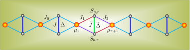
Figure 1: Schematic representation of the spin-1/2 Ising-$XXZ$ diamond chain with distorted impurity. The Ising spins are denoted by $\mu_{i}$ and the Heisenberg spins are represented by $S_{a(b),i}$

$$\begin{array}[]{cl}\mathcal{H}_{i}^{imp}=&\widetilde{J}\left(\mathbf{S}_{a,i},\mathbf{S}_{b,i}\right)_{\widetilde{\Delta}}+\left(J_{1}\mu_{i}+J_{2}\mu_{i+1}\right)S_{a,i}^{z}+\left(J_{1}\mu_{i+1}+J_{2}\mu_{i}\right)S_{b,i}^{z}\\ &-B\left(S_{a,i}^{z}+S_{a,i}^{z}\right)-\frac{B}{2}\left(\mu_{i}+\mu_{i+1}\right),\\ &\mathrm{for}\>i=r,\end{array}$$

is the Hamiltonian of the impurity. Here $J_{1}=J_{0}(1+\eta)$, $J_{2}=J_{0}(1.0+\gamma)$, $\widetilde{J}=J(1.0+\alpha)$, $\widetilde{\Delta}=\Delta(1.0+\Omega)$ represents the impurity parameters. Throughout the text, the symbol   $\widetilde{}$   on the parameter indicates that this parameter is related to impurity in the chain.

The eigenvalues of $\mathcal{H}_{i}^{host}$ is given by

$$\begin{array}[]{cl}\varepsilon_{1,4}=&\frac{J\Delta}{4}\pm\left(J_{0}\mp\frac{B}{2}\right)\left(\mu_{i}+\mu_{i+1}\right)\mp\frac{B}{2},\\ \varepsilon_{2,3}=&-\frac{J\Delta}{4}\pm\frac{J}{2}-\frac{B}{2}\left(\mu_{i}+\mu_{i+1}\right),\end{array}$$

and the corresponding eigenvectors are

$$|\varphi_{i1}\rangle = |00\rangle_{i},$$ (2)

$$|\varphi_{i2,i3}\rangle = \frac{1}{\sqrt{2}}\left(|01\rangle_{i}\pm|10\rangle_{i}\right),$$ (3)

$$|\varphi_{i1}\rangle = |11\rangle_{i}.$$ (4)

Likewise eigenvalues of $\mathcal{H}_{i}^{imp}$ is given by

$$\begin{array}[]{cl}\widetilde{\varepsilon}_{1,4}=&\frac{\widetilde{J}\widetilde{\Delta}}{4}\pm\left(\frac{(J_{1}+J_{2})}{2}\mp\frac{B}{2}\right)\left(\mu_{r}+\mu_{r+1}\right)\mp B,\\ \widetilde{\varepsilon}_{2,3}=&-\frac{\widetilde{J}\widetilde{\Delta}}{4}-\frac{B}{2}\left(\mu_{r}+\mu_{r+1}\right)\pm\frac{1}{2}\sqrt{\Sigma^{2}+\widetilde{J}^{2}},\end{array}$$

where $\Sigma=\left(J_{1}-J_{2}\right)\left(\mu_{r}-\mu_{r+1}\right)$. The corresponding eigenvectors are given by

$$|\widetilde{\varphi}_{r1}\rangle = |00\rangle_{r},$$ (5)

$$|\widetilde{\varphi}_{r2,r3}\rangle = M_{\pm}|01\rangle_{r}+N_{\pm}|10\rangle_{r},$$ (6)

$$|\widetilde{\varphi}_{r4}\rangle = |11\rangle_{r},$$ (7)

where

$$M_{\pm}=\frac{\widetilde{J}}{\sqrt{2\widetilde{J}^{2}+2\Sigma^{2}\mp 2\Sigma\sqrt{\Sigma^{2}+\widetilde{J}^{2}}}},$$

and

$$N_{\pm}=\frac{-\Sigma\pm\sqrt{\Sigma^{2}+\widetilde{J}^{2}}}{\sqrt{2\widetilde{J}^{2}+2\Sigma^{2}\mp 2\Sigma\sqrt{\Sigma^{2}+\widetilde{J}^{2}}}}.$$

Notice that, in general $J_{1}\neq J_{2}$, therefore $\mathcal{H}_{i}^{imp}$ has diferent eigenvector from $\mathcal{H}_{i}^{host}.$ In addition, the probabilities of obtaining $|01\rangle_{r}$ and $|10\rangle_{r}$ are different in eigenstate $|\widetilde{\varphi}_{r2,r3}\rangle$. This is the main difference between our results and those presented in previous works moi ; mr ; mro .

II.1 The partition function

The state at thermal equilibrium can be described by the Gibb’s density operators $\rho(T)=\frac{\exp(-\beta\mathcal{H})}{Z}$, where $\beta=1/k_{B}T$, with $k_{B}$ being the Boltzmann’s constant, $T$ is the absolute temperature, whereas the partition function of the system is defined by $Z=Tr\left[\exp(-\beta\mathcal{H})\right]$. Similarly to that made by Freitas $\mathit{et\,al}$ mro we consider the chain with periodic boundary condition and use the transfer-matrix notation to obtain the partition function. Thus

$$\begin{array}[]{cl}Z=&\sum_{\{\mu\}}w(\mu_{1},\mu_{2})...w(\mu_{r-1},\mu{r})\widetilde{w}(\mu_{r},\mu_{r+1})w(\mu_{r+1},\mu_{r+2})...w(\mu_{N},\mu_{1}),\end{array}$$

where

$$w(\mu_{i},\mu_{i+1})=\sum_{j=1}^{4}e^{-\beta\epsilon_{ij}(\mu_{i},\mu_{i+1})},$$ (8)

and

$$\widetilde{w}(\mu_{i},\mu_{i+1})=\sum_{j=1}^{4}e^{-\beta\widetilde{\epsilon}_{ij}(\mu_{i},\mu_{i+1})}.$$ (9)

The partition function can be simplified by taking $Z=\mathrm{Tr}(\widetilde{W}W^{N-1})$, in such a way that

$$W=\left[\begin{array}[]{cc}w(\frac{1}{2},\frac{1}{2})&w(\frac{1}{2},-\frac{1}{2})\\ w(-\frac{1}{2},\frac{1}{2})&w(-\frac{1}{2},-\frac{1}{2})\end{array}\right],$$

and

$$\widetilde{W}=\left[\begin{array}[]{cc}\widetilde{w}(\frac{1}{2},\frac{1}{2})&\widetilde{w}(\frac{1}{2},-\frac{1}{2})\\ \widetilde{w}(-\frac{1}{2},\frac{1}{2})&\widetilde{w}(-\frac{1}{2},-\frac{1}{2})\end{array}\right].$$

In order to simplify the notation we will start to denote $w_{\pm\pm}\equiv w(\pm\frac{1}{2},\pm\frac{1}{2})$ and $w_{\pm\mp}\equiv w(\pm\frac{1}{2},\mp\frac{1}{2})$. Through the diagonalization of the transfer-matrix we obtain

$$Z=a\Lambda_{+}^{N-1}+d\Lambda_{-}^{N-1},$$ (10)

where

$$\Lambda_{\pm}=\frac{w_{++}+w_{--}\pm Q}{2}$$

with $Q=\sqrt{(w_{++}-w_{--})^{2}+4w_{+-}^{2}}$ are the eigenvalues associated with the matrix W. Furthermore

$$a=\frac{4w_{+-}\widetilde{w}_{+-}+(w_{++}-w{--})(\widetilde{w}_{++}-\widetilde{w}_{--})+Q(\widetilde{w}_{++}+\widetilde{w}_{--})}{2Q},$$ (11)

and

$$d=\frac{-4w_{+-}\widetilde{w}_{+-}-(w_{++}-w{--})(\widetilde{w}_{++}-\widetilde{w}_{--})+Q(\widetilde{w}_{++}+\widetilde{w}_{--})}{2Q}.$$ (12)

At the thermodynamic limit, $N\rightarrow\infty$, we have

$$Z=a\Lambda_{+}^{N-1},$$

since $a\Lambda_{+}^{N-1}>d\Lambda_{-}^{N-1}.$

II.2 Average reduced density operator

In order to obtain the reduced density matrix let’s take the thermal average for each two-qubit Heisenbergmr ; mro ,. We start by defining the operator as a function of spin particles $\mu_{i}$ and $\mu_{i+1}$

$$\varrho(\mu_{i},\mu_{i+1})=\sum_{i=1}^{4}e^{-\beta\epsilon_{i,j}}|\phi_{i,j}\rangle\langle\phi_{i,j}|.$$ (13)

For impurity we define the operator $\widetilde{\varrho}$ of the two-qubit Heisenberg operator

$$\widetilde{\varrho}(\mu_{r},\mu_{r+1})=\left[\begin{array}[]{cccc}\widetilde{\varrho}_{1,1}&0&0&0\\ 0&\widetilde{\varrho}_{2,2}&\widetilde{\varrho}_{2,3}&0\\ 0&\widetilde{\varrho}_{3,2}&\widetilde{\varrho}_{3,3}&0\\ 0&0&0&\widetilde{\varrho}_{4,4}\end{array}\right],$$

where

$$\begin{array}[]{cl}\widetilde{\varrho}_{1,1}(\mu_{r},\mu_{r+1})=&\mathrm{e}^{-\beta\widetilde{\varepsilon}_{r1}},\\ \widetilde{\varrho}_{2,2}(\mu_{r},\mu_{r+1})=&\mathrm{e}^{-\beta\widetilde{\varepsilon}_{r2}}M_{+}^{2}+\mathrm{e}^{-\beta\widetilde{\varepsilon}_{r3}}M_{-}^{2},\\ \widetilde{\varrho}_{2,3}(\mu_{r},\mu_{r+1})=&\mathrm{e}^{-\beta\widetilde{\varepsilon}_{r2}}M_{+}N_{+}+\mathrm{e}^{-\beta\widetilde{\varepsilon}_{r3}}M_{-}N_{-},\\ \widetilde{\varrho}_{4,4}(\mu_{r},\mu_{r+1})=&\mathrm{e}^{-\beta\widetilde{\varepsilon}_{r4}}.\end{array}$$

Using the transfer-matrix approach we can write the elements of the density matrix for impurity $\widetilde{\rho}_{k,l}$ in the form mro

$$\widetilde{\rho}_{k,l}=\frac{1}{Z}\mathrm{Tr}\left(\widetilde{P}_{k,l}W^{N-1}\right),$$ (14)

where

$$\widetilde{P}_{k,l}=\left[\begin{array}[]{cc}\widetilde{\rho}_{k,l}(\frac{1}{2},\frac{1}{2})&\widetilde{\rho}_{k,l}(\frac{1}{2},-\frac{1}{2})\\ \widetilde{\rho}_{k,l}(-\frac{1}{2},\frac{1}{2})&\widetilde{\rho}_{k,l}(-\frac{1}{2},-\frac{1}{2})\end{array}\right],$$

consider $\widetilde{\rho}_{k,l}(\pm\pm)\equiv\widetilde{\rho}_{k,l}(\pm\frac{1}{2},\pm\frac{1}{2})$ and $\widetilde{\rho}_{k,l}(\pm\mp)\equiv\widetilde{\rho}_{k,l}(\pm\frac{1}{2},\mp\frac{1}{2})$. Being $U$ the matrix that diagonalizes $W$ we can rewrite Eq. (14) in the form

$$\begin{array}[]{ccc}\widetilde{\rho}_{k,l}&=&\frac{\mathrm{Tr}\left(U^{-1}\widetilde{P}_{k,l}U\left[\begin{array}[]{cc}\Lambda_{+}^{N-1}&0\\ 0&\Lambda_{-}^{N-1}\end{array}\right]\right)}{a\Lambda_{+}^{N-1}+d\Lambda_{-}^{N-1}},\end{array}$$

that at the thermodynamic limit, $N\rightarrow\infty$, it reduces to

$$\begin{array}[]{ccc}\widetilde{\rho}_{k,l}&=&\frac{\mathcal{A}_{k,l}+\mathcal{B}_{k,l}}{\mathcal{M}_{k,l}},\end{array}$$

where

$$\begin{array}[]{cl}\mathcal{A}_{k,l}=&Q\left[\widetilde{\varrho}_{k,l}(++)+\widetilde{\varrho}_{k,l}(--)\right]+4w_{+-}\widetilde{\varrho}_{k,l}(+-)\\ \mathcal{B}_{k,l}=&\left[\widetilde{\varrho}_{k,l}(++)-\widetilde{\varrho}_{k,l}(--)\right]\left(w_{++}-w_{--}\right)\\ \mathcal{M}=&Q\left(\widetilde{w}_{++}+\widetilde{w}_{--}\right)+4w_{+-}\widetilde{w}_{+-}+\left(\widetilde{w}_{++}-\widetilde{w}_{--}\right)\left(w_{++}-w_{--}\right).\end{array}$$

Finally, we conclude that the elements of the reduced density matrix take the form

$$\widetilde{\rho}(T)=\left[\begin{array}[]{cccc}\widetilde{\rho}_{11}&0&0&0\\ 0&\widetilde{\rho}_{22}&\widetilde{\rho}_{23}&0\\ 0&\widetilde{\rho}_{23}&\widetilde{\rho}_{33}&0\\ 0&0&0&\widetilde{\rho}_{44}\end{array}\right].$$ (15)

The state at thermal equilibrium can be described by the Gibb’s density operators $\rho(T)$ represents a thermal density operator, the entanglement in the thermal state is simply called thermal entanglement.

III Quantum Correlations

In order to describe the thermal entanglement of two-qubit system, the concurrence is used as a measure of the entanglement. The concurrence $\mathcal{C}$ is defined as wootters

$$\mathcal{C}={\rm{max}\left\{0,\sqrt{\lambda_{1}}-\sqrt{\lambda_{2}}-\sqrt{\lambda_{3}}-\sqrt{\lambda_{4}}\right\},}$$

where $\lambda_{i}\>(i=1,2,3,4)$ are the eigenvalues in decreasing order of the matrix

$$R=\rho\left(\sigma^{y}\otimes\sigma^{y}\right)\rho^{\ast}\left(\sigma^{y}\otimes\sigma^{y}\right),$$

with $\sigma^{y}$ being the Pauli matrix. We will explore the thermal entanglement of the model. To this end, we should obtain the eigenvalues of $R$. Thus, the concurrence $\mathcal{C}$ can be written as

$$\mathcal{C}(\widetilde{\rho})=2\mathrm{max}\{|\widetilde{\rho}_{2,3}|-\sqrt{\widetilde{\rho}_{1,1}\widetilde{\rho}_{4,4}},0\}\;.$$

In this case, the analytical expression of the thermal concurrence is too large to be explicitly provided in this paper.

In addition to entanglement, the system may also have other quantum correlations, such as quantum discord. Quantum coherence is more robust than entanglement, so it can be a key ingredient in the development of quantum information. We calculate the quantum coherence by the $l_{1}$-norm defined by the sum of the absolute values of the elements off the main diagonal of the reduced density operator of the system baum . So

$$\mathcal{C}_{l_{1}}(\rho)=\sum_{i\neq j}|\langle i|\rho|j\rangle|.$$

III.1 Concurrence

In our model $J_{1}$ and $J_{2}$ they can be taken independently. This guarantees a much greater generality of this model in relation to those previously studied moi ; mr ; mro . This greater generality is of great interest in experimental measurements since it allows greater flexibility in modeling.

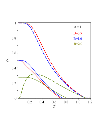
Figure 2: The concurrence $\mathcal{C}$ as a function of temperature $T$ for $J_{0}/J=1.0$, $\Delta=1.0$, $\alpha=0.0$, solid curve ($\eta=0.0$, $\gamma=0.0$, $\Omega=0.0$), dashed curve ($\eta=-0.5$, $\gamma=-0.6$, $\Omega=0.8$).

With an appropriate choice of parameters, we can obtain optimal entanglement results. In Fig. 2, we show the concurrence $\mathcal{C}$ as a function of temperature $T$ and for different values of magnetic field. The solid curve indicates the original model (without impurity) while the dashed curve indicates the model with impurity described by the Hamiltonian $\mathcal{H}$. In addition, the red curve refers to a magnetic field $B=1.0$ and the blue curve refers to $B=2.0$. For the impurity model, the adopted parameters were ($\eta=-0.5$, $\gamma=-0.6$, $\Omega=0.8$). In relation to the original model moi , we can clearly see the advantage of the model with impurity. The impurity model presents greater entanglement and also a greater critical entanglement temperature. For higher fields we can observe a different behavior for the two models. In this case, the entanglement in the model with impurity is zero for $T=0.0$ and different from zero for higher temperatures, until it becomes null at the critical entanglement temperature. In this case, the triplet splits and $|\widetilde{\varphi}_{r_{1},r_{2}}\rangle$ becames the ground states. In this case there is no entanglement at $T=0.0$. But the increase in temperature increases entanglement by bringing in some singlet component into the mixture.

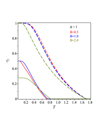
Figure 3: The concurrence $\mathcal{C}$ as a function of the temperature $T$, $J_{0}/J=1.0$ , $\Delta=1.0$, solid curve(original model), dashed curve ($\alpha=0.5$, $\eta=-0.5$, $\gamma=-0.6$, $\Omega=0.8$).

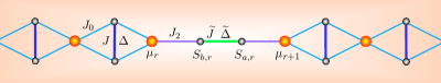
Figure 4: Schematic representation of the form taken by the impurity when we take $\eta=-1.0$ ($J_{1}=0.0$). Note that instead of the diamond shape, the impurity structure now takes on a horizontal shape.

In Figure 3 we analyze how a change in the interaction between the spins of the impurity affects the entanglement. This interaction is represented by $\widetilde{J}$ and was obtained by taking $\alpha=0.5$. In other words, the interaction between the Heisenberg spins in the impurity was greater than between the Heisenberg spins in the rest of the chain. The advantage of this small modification is evident in relation to the situation analyzed in Figure 2. In this case we can see that the entanglement is different from zero even for high field. In addition, the increase in the critical entanglement temperature was very significant compared to the original model (solid curve).

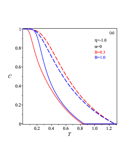
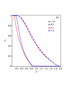
Figure 5: The concurrence $\mathcal{C}$ as a function of the temperature $T$, we set $J_{0}/J=1.0$, $\Delta=1.3$, $\eta=-1.0$, (a) dashed curve ($\alpha=0.0$, $\gamma=-0.8$, $\Omega=0.8$), (b) dashed curve ($\alpha=0.5$, $\gamma=-0.8$, $\Omega=0.8$)

We observe an interesting behavior in the system when we take $J_{1}=0.0$ or $\eta=-1.0$. This condition is equivalent to a change in the structure of the impurity. Instead of the diamond shape shown in Figure 1, the impurity term have a horizontal interaction as shown in Figure 4. This situation is analyzed in Figure 5 with the following parameters $J_{0}/J=1.0$, $\Delta=1.3$, $\eta=-1.0$. In Figure 5(a) we considered $\alpha=0.0$ ($J=\widetilde{J}$) and we observed entanglement and critical entanglement temperature higher than the original model (solid curve). In Figure 3 we see an increase in entanglement with $\alpha=0.5$, the same we observed in this case. In Figure 5 (b) is possible observe the entanglement gain in relation to the original model (solid curve), both for low and high fields.

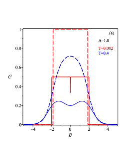
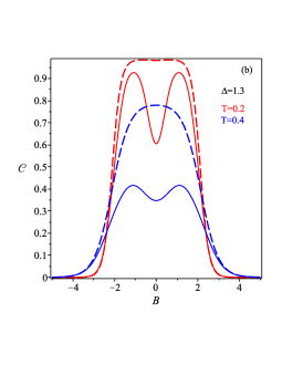
Figure 6: The concurrence $\mathcal{C}$ as a function of the magnetic field $B$, we set $J_{0}/J=1.0$, $\alpha=0.0$, $\eta=-0.5$, $\gamma=-0.6$, $\Omega=0.8$. (a) dashed curve ($\Delta=1.0$, $T=0.002$, $T=0.400$), (b) dashed curve ($\Delta=1.3$, $T=0.200$, $T=0.400$)

Our results also show that with an appropriate choice of parameters our model presents more robust entanglement for application of magnetic field than the original model. In figure 6 we present some curves of the concurrence as a function of the magnetic field. As before, here solid curves refer to the original model and the dashed curves refer to the current model. Although the critical magnetic field (above which the entanglement is zero) is the same for both models, the entanglement is significantly greater in the current model.

III.2 $l_{1}$-norm

Here we will discuss the results regarding the calculation of quantum coherence using the $l_{1}$-norm. In Figure 7 we adopt the same parameters adopted in Figure 2. The comparison between the two Figures is instructive. The behavior of the curves is similar in the two Figures. Again there is a clear advantage of the model with impurity (dashed curve) compared to the original model(solid curve). The main difference is in the scale of magnitude. Quantum coherence $\mathcal{C}_{l_{1}}$ is significantly greater than concurrence. This result is not surprising since coherence measures, in addition to entanglement, other quantum correlations. Coherence is a basis-dependent measure and states without any quantum correlations can be fully coherent on an orthogonal basis. In addition, coherence is present also in single pure quantum systems which does not share any correlation with other systems.

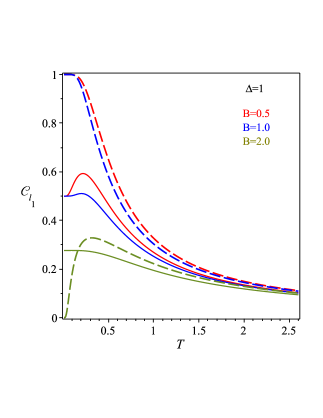
Figure 7: The quantum coherence $\mathcal{C}_{l_{1}}$ as a function of temperature $T$ for $J_{0}/J=1.0$, $\Delta=1.0$, $\alpha=0.0$, solid curve (original model), dashed curve ($\eta=-0.5$, $\gamma=-0.6$, $\Omega=0.8$).

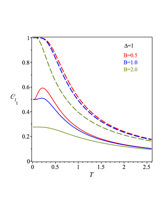
Figure 8: The quantum coherence $\mathcal{C}_{l_{1}}$ as a function of temperature $T$ for $J_{0}/J=1.0$, $\Delta=1.0$, solid curve (original model), dashed curve ($\alpha=0.5$, $\eta=-0.5$, $\gamma=-0.6$, $\Omega=0.8$).

Analogous to what was done in Figure 3, in Figure 8 we analyze how a change in the interaction between the spins of the impurity affects the coherence $\mathcal{C}_{l_{1}}$. As with concurrence, the increase in coherence with this small change was very significant. The coherence of the impurity is greater than $0.2$ up to the temperature of $2.5$ for all fields presented. The change in $\widetilde{J}$ provides considerable gain in both concurrence and coherence.

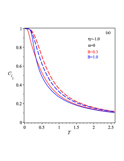
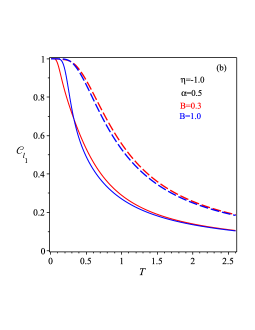
Figure 9: The concurrence $\mathcal{C}_{l_{1}}$ as a function of the temperature $T$, we set $J_{0}/J=1.0$, $\Delta=1.3$, $\eta=-1.0$, (a) dashed curve ($\alpha=0.0$, $\gamma=-0.8$, $\Omega=0.8$), (b) dashed curve ($\alpha=0.5$, $\gamma=-0.8$, $\Omega=0.8$)

In Figure 9 we will analyze the coherence by taking the parameter $J_{1}=0.0$. It is interesting to note that in this case the coherence of the original model and the model with impurity are close when we take the parameter $\alpha=0.0$ (Figure 9(a)). From Figure 5 it is evident that the same does not occur with concurrence. This allows us to conclude that in this case the coherence is proportionally greater than the concurrence in the original model than in the model with impurity. In Figure 9(b) we can see the gain in coherence in relation to the original model increasing the interaction between Heisenberg spins in impurity ($\alpha=0.5$).

IV Quantum teleportation

In this section, we study the quantum teleportation via a distorted Ising-$XXZ$ diamond chain using the standard teleportation protocol. By means of an entangled mixed state as resource, the standard teleportation can be regarded as a general depolarizing channel peres with probabilities given by the maximally entangled components of the resource. An unknown two-qubit pure state to be teleported can be written as $|\psi_{in}\rangle=\cos\left(\frac{\theta}{2}\right)|10\rangle+e^{i\phi}\sin\left(\frac{\theta}{2}\right)|01\rangle\;$, where $0\leq\theta\leq\pi$ and $0\leq\phi\leq 2\pi$. In the density operator formalism, the concurrence $\mathcal{C}_{in}$ of the input state, can be written as

$$\mathcal{C}_{in}=2|e^{i\phi}\sin\left(\frac{\theta}{2}\right)\cos\left(\frac{\theta}{2}\right)|=|\sin(\theta)|\;.$$

When a two-qubit state $\rho_{in}$ is teleported via the mixed channel $\widetilde{\rho}_{ch}$, then the output state $\widetilde{\rho}_{out}$ is given by peres

$$\widetilde{\rho}_{out}=\sum_{i,j=\left\{0,x,y,z\right\}}p_{i}p_{j}\left(\sigma_{i}\otimes\sigma_{j}\right)\rho_{in}\left(\sigma_{i}\otimes\sigma_{j}\right)\;,$$

in which $p_{i}=tr\left[E^{i}\widetilde{\rho}_{ch}\right]$, $E^{0}=|\Psi^{-}\rangle\langle\Psi^{-}|$, $E^{1}=|\Phi^{-}\rangle\langle\Phi^{-}|$, $E^{2}=|\Phi^{+}\rangle\langle\Phi^{+}|$ and $E^{3}=|\Psi^{+}\rangle\langle\Psi^{+}|$, where $|\Phi^{\pm}\rangle=\frac{1}{\sqrt{2}}\left(|00\rangle\pm|11\rangle\right)$ and $|\Psi^{\pm}\rangle=\frac{1}{\sqrt{2}}\left(|01\rangle\pm|10\rangle\right)$ are Bell states. Here, we consider the density operator channel as $\widetilde{\rho}_{ch}\equiv\widetilde{\rho}(T)$. Then the output density operator $\widetilde{\rho}_{out}$ is given by

$$\widetilde{\rho}_{out}=\left[\begin{array}[]{cccc}c&0&0&0\\ 0&f&\chi&0\\ 0&\chi&g&0\\ 0&0&0&c\end{array}\right]\;.$$ (16)

The elements of the operators can be expressed as

$$\begin{array}[]{cl}c=&\left(\widetilde{\rho}_{2,2}+\widetilde{\rho}_{3,3}\right)\left(\widetilde{\rho}_{1,1}+\widetilde{\rho}_{4,4}\right),\\ f=&\left(\widetilde{\rho}_{1,1}+\widetilde{\rho}_{4,4}\right)^{2}\cos^{2}\left(\frac{\theta}{2}\right)+\left(\widetilde{\rho}_{2,2}+\widetilde{\rho}_{3,3}\right)^{2}\sin^{2}\left(\frac{\theta}{2}\right),\\ g=&\left(\widetilde{\rho}_{2,2}+\widetilde{\rho}_{3,3}\right)^{2}\cos^{2}\left(\frac{\theta}{2}\right)+\left(\widetilde{\rho}_{1,1}+\widetilde{\rho}_{4,4}\right)^{2}\sin^{2}\left(\frac{\theta}{2}\right),\\ \chi=&2e^{i\phi}\widetilde{\rho}_{2,3}^{\,2}\sin\theta.\end{array}$$

According to the definition, the concurrence of the input state is given as $\mathcal{C}_{in}=\sin(\frac{\theta}{2})$, and the output one follows by

$$\mathcal{C}_{out}(\widetilde{\rho})=2max\left\{2\widetilde{\rho}_{2,3}^{\,2}\mathcal{C}_{in}-2|\widetilde{\rho}_{2,2}||\widetilde{\rho}_{1,1}-\widetilde{\rho}_{4,4}|,0\right\}.$$

More recently, the teleportation of the same entangled state was studies in this model without impurities tele and with impurities mro .

V Average fidelity of teleportation

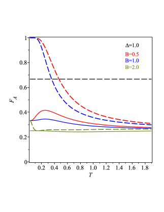
Figure 10: The average fidelity $F_{A}$ as a function of temperature $T$ for $J_{0}/J=1.0$, $\Delta=1.0$, solid curve (original model), dashed curve ($\alpha=0.0$, $\eta=-0.5$, $\gamma=-0.6$, $\Omega=0.8$).

In the following discussion, we turn our attention to the quality of the entanglement teleportation. The quality of the teleportation is measurement by the fidelity between the input state $\rho_{in}$ and the output state $\rho_{out}$. If the input state is pure, the fidelity can be written as

$$F=\langle\psi_{in}|\rho_{out}|\psi_{in}\rangle\;.$$

For this model $F$ can be written as

$$\begin{array}[]{cl}F=&\frac{\sin^{2}\theta}{2}\left[\left(\widetilde{\rho}_{1,1}+\widetilde{\rho}_{4,4}\right)^{2}+4\widetilde{\rho}_{2,3}^{\,2}-\left(\widetilde{\rho}_{2,2}+\widetilde{\rho}_{3,3}\right)^{\,2}\right]+\left(\widetilde{\rho}_{2,2}+\widetilde{\rho}_{3,3}\right)^{\,2}.\end{array}$$

In general the state to be teleported is unknown, it is more useful to calculate the average fidelity. Thus the average fidelity of teleportation can be formulated as

$$F_{A}=\frac{1}{4\pi}\intop_{0}^{2\pi}d\phi\intop_{0}^{\pi}F\sin\theta d\theta\;.$$

The average fidelity of teleportation can be written as

$$\begin{array}[]{cl}F_{A}=&\frac{1}{3}\left[\left(\widetilde{\rho}_{1,1}+\widetilde{\rho}_{4,4}\right)^{2}+4\widetilde{\rho}_{2,3}^{\,2}-\left(\widetilde{\rho}_{2,2}+\widetilde{\rho}_{3,3}\right)^{\,2}\right]+\left(\widetilde{\rho}_{2,2}+\widetilde{\rho}_{3,3}\right)^{\,2}.\end{array}$$

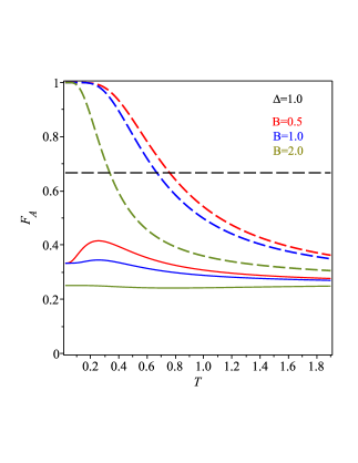
Figure 11: The average fidelity ${F}_{A}$ as a function of temperature $T$ for $J_{0}/J=1.0$, $\Delta=1.0$, solid curve (original model), dashed curve ($\alpha=0.5$, $\eta=-0.5$, $\gamma=-0.6$, $\Omega=0.8$).

To transmit a quantum state $|\psi_{in}\rangle\;$ better than any classical communication protocol, $F_{A}$ must be great than $\frac{2}{3}$ which is the best fidelity in the classical world joz . To demonstrate the effects of the impurity on the average fidelity, we plot the behavior of average fidelity. In Fig. 10, we show the average teleportation $F_{A}$ as a function of temperature $T$ for $J_{0}/J=1.0$, $\Delta=1.0$ and several values of magnetic field. For the model with impurity, we set $\alpha=0.5$, $\eta=-0.5$, $\gamma=-0.6$, $\Omega=0.8$. The horizontal dashed lines at $F_{A}=\frac{2}{3}$ denote the limit of quantum fidelities. We can see that in the original model the average fidelity is below $\frac{2}{3}$, signaling that it is not possible to teleport information. Meanwhile, when consider the impurity, we have a considerable improvement in quantum teleportation. For weak magnetic field, the average fidelity reaches maximum value at low temperatures as the temperature increases, the average fidelity decays up to the critical temperature, beyond which the teleportation of information is no longer valid. On the other hand, for strong magnetic field, the effect of the impurity on the quantum teleportation does not occurs. It means that, average fidelity remains below $\frac{2}{3}$ regardless of the temperature rise.

In Fig. 11, the behavior of the average fidelity as a function of temperature $T$ with fixed parameters values, $J_{0}/J=1.0$, $\Delta=1.0$ $\eta=-0.5$, $\gamma=-0.6$, $\Omega=0.8$ and different values of magnetic field $B$ is depicted. In this figure, we also consider the impurity in the parameter $\alpha$ of Heisenberg exchange interaction, we select $\alpha=0.5$, under this condition a considerable increase in average fidelity is observed, reaching its maximum value $F_{A}=1$ for several values of magnetic field, including strong magnetic fields (dashed curves). After that, it gradually decreases with increase the temperature. However, the average fidelity is always less than $F_{A}<\frac{2}{3}$ for original model (solid curves), that is, in this case the quantum teleportation fails. All these show again that considerable enhancement of teleportation can be achieved by tuning the strenght of impurity parameters.

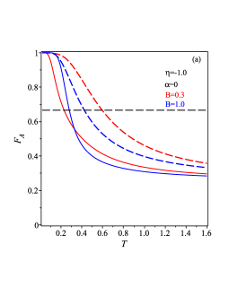
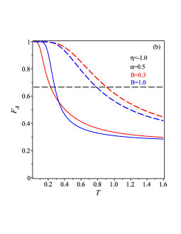
Figure 12: The average fidelity $F_{A}$ as a function of the temperature $T$, we set $J_{0}/J=1.0$, $\Delta=1.3$, $\eta=-1.0$, (a) dashed curve ($\alpha=0.0$, $\gamma=-0.8$, $\Omega=0.8$), (b) dashed curve ($\alpha=0.5$, $\gamma=-0.8$, $\Omega=0.8$)

Finally, in Fig. 12, let us study the behavior of the system in extreme cases. We analyze the case when $J_{1}=0.0$ or $\eta=-1.0$ which corresponds to collapse of one of the impurities of the Ising-like interaction, as depicted in Fig. 4. We set $J_{0}/J=1.0$, $\Delta=1.3$. In Fig. 12(a), we illustrate the average fidelity as a function of temperature $T$ for different values of the magnetic field and the fixed values of impurities parameters $\alpha=0.0$, $\gamma=-0.8$, $\Omega=0.8$. As can be seen, the results of $F_{A}$ indicate that, for low temperatures, the average fidelity is maximum, that is, $F_{A}=1$, for both models. However, for the higher temperature, average fidelity with impurity is more robust in comparison to that without it.

On the other hand, Fig. 12(b) shows the average fidelity for two values of magnetic field and we fixed $\alpha=0.5$, $\gamma=-0.8$, $\Omega=0.8$. This figure shows clearly that the behavior the average fidelity is even more robust when we consider the impurity in the Heisenberg spin exchange parameter $\alpha=0.5$, allowing the teleportation of information at higher temperature. Altogether, it could be concluded that impurity generated by a local bound disorder of the interchain exchange coupling affects strongly the quantum correlations, which generates a considerable increase in the teleportation of information.

VI Conclusions

In summary, we have investigated the effects due to the inclusion of an distorted impurity plaquette on the spin-1/2 Ising-$XXZ$ diamond chain. Next, the quantum correlations and teleportation of the model under investigation have been exactly calculated using the transfer-matrix technique. In particular, our attention has been paid to a rigorous analysis of the quantum correlations of the interstitial distorted impurity Heisenberg dimers through the concurrence and norm-$l_{1}$. We observed that the impurity strongly influence at the behavior of the entanglement and quantum coherence. More specifically, the results show the existence of the thermal entanglement and quantum thermal coherence in regions beyond the reach of the original model. One of our notable results is that quantum correlations can be controlled and tuned by Ising and Heisenberg parameters into model.

In addition, we have also discussed the teleportation of the two-qubits in an arbitrary state through a quantum channel composed by a couple of Heisenberg dimers with distorted impurity in an Ising-$XXZ$ diamond chain structure. We have found that, the quantum teleportation increases when increases some suitable impurity parameters. The influence of impurity is more evident in the average fidelity when we consider the impurity in the Heisenberg parameter.

Finally, our results show that the impurities can be manipulated to locally control the thermal quantum correlations, unlike the original model where it is done globally.

References

• (1) C. H. Bennett, G. Brassard, C. CrΓ©peau, R. Jozsa, A. Peres, W. K. Wootters, Phys. Rev. Lett. 70, 1895 (1993).
• (2) C. H. Bennett, H. J. Bernstein $\mathit{et\,al}$, Phys. Rev. A 53, 2046 (1996).
• (3) L. Amico, R. Fazio, A. Osterloh and V. Vedral, Rev. Mod. Phys. 80, 517 (2008).
• (4) J. I. Cirac, P. Zoller, Nature, 404, 579 (2000).
• (5) D. Loss, D. P. DiVincenzo, Phys. Rev. A 57, 120 (1998).
• (6) T. J. G. Apollaro, G. M. A. Almeida, S. Lorenzo, A. Ferraro, S. Piganelli, Phys. Rev A 100, 052308 (2019).
• (7) M. C. Amesen, S. Bose, V. Vedral, Phys. Rev. Lett. 87, 017901 (2001).
• (8) D. P. DiVincenzo, D. Bacon, J. Kempe, G. Burkard and K. B. Whaley, Nature, 408, 339 (2000).
• (9) S. Bose, Phys. Rev. Lett. 91, 207901 (2003).
• (10) G. L. Kamta, A. F. Starace, Phys. Rev. Lett. 88, 107901 (2002).
• (11) L. Zhou, H. S. Song, Y. Q. Guo, C. Li, Phys. Rev. Lett. 68, 024301 (2003).
• (12) F. Levi, F. Mintert, New J. Phys. 16, 033007 (2014).
• (13) A. Streltsov, G. Adesso, M. B. Plenio, Rev. Mod. Phys. 89, 041003 (2017).
• (14) A. Winter, D. Yang, Phys. Rev. Lett. 116, 120404 (2016).
• (15) G. Karpat, B. Γ‡akmak, F. Fanchini, Phys. Rev. B 90, 104431 (2014).
• (16) W. Wu, J. Xu, Phys. Lett. A 381, 239 (2017).
• (17) T. Baumgratz, M. Cramer, M. B. Plenio, Phys. Rev. Lett. 113, 140401 (2014).
• (18) M. L. Hu, X. Hu, J. C. Wang, Y. Peng, Y. R. Zhang, H. Fan, Phys. Rep. 762, 1 (2018).
• (19) Z. Xi, Y. Li, H. Fan, Sci. Rep. 5, 10922 (2015).
• (20) K. C. Tan, H. Kwon, C. -Y. Park, H. Jeong, Phys. Rev. A 94, 022329 (2016).
• (21) H. Kikuchi, Y. Fujii, M. Chiba, S. Mitsudo, T. Idehara, Phys. B 329, 967 (2003).
• (22) L. CanovΓ‘, J. Strecka, M. Jascur, J. Phys.: Condens. Matter 18, 4967 (2006).
• (23) B. Lisnyi, J. Strecka, Phys. Status Solidi B 251, 1083 (2014).
• (24) J. S. Valverde, O. Rojas, S. M. de Souza, J. Phys.: Condens. Matter 20, 345208 (2008).
• (25) O. Rojas, M. Rojas, N. S. Ananikian, S. M. de Souza, Phys. Rev. A 86, 042330 (2012).
• (26) J. Torrico, M. Rojas, S. M. de Souza, Onofre Rojas, N. S. Ananikian, Europhys. Lett. 108, 50007 (2014).
• (27) J. Torrico, M. Rojas, M. S. S. Pereira, J. Strecka, M. L. Lyra, Phys. Rev. B 93, 014428 (2016).
• (28) I. M. Carvalho, J. Torrico, S. M. de Souza, M. Rojas, O. Rojas, J. Magn. Magn. Matter. 465, 323 (2018).
• (29) K. Gao, Y.-L. Xu, X.-M. Kong, Z.-Q. Liu, Physica A 429, 10 (2015).
• (30) W. W. Cheng, X. Y. Wang, Y. B. Sheng, L. Y. Gong, S. M. Yhao, J. M. Liu, Sci. Rep. 7, 42360 (2017).
• (31) M. Rojas, S. M. de Souza, O. Rojas, Ann. Phys. 377, 506 (2017).
• (32) H. Falk, Phys. Rev. 151, 304 (1966).
• (33) T. J. G. Apollaro, F. Plastina, L. Banchi, A. Cuccoli, R. Vaia, P. Verrucchi, M. Paternostro, Phys. Rev. A 88, 052336 (2013).
• (34) H. Saleur, P. Schmitteckert, R. Vasseur, Phys. Rev. B 88, 085413 (2013).
• (35) O. Osenda, Z. Huang, S. Kais, Phys. Rev. A 67, 062321 (2003).
• (36) E. Solano-Carrillo, R. Franco, J. Silva-Valencia, Physica A 390, 2208 (2011).
• (37) Y. Sun, X. Huang, G. Min, Phys. Lett. A 381, 387 (2017).
• (38) T. J. Apollaro, A. Cuccoli, A. Fubini, F. Plastina, P. Verrucchi, Phys. Rev. A 77, 062314 (2008).
• (39) J. -M. Gong, Z. -Q. Hui, Physica B 444, 40 (2014).
• (40) M. -L. Hu, X. -Q. Xi, Opt. Commun. 282, 4819 (2009).
• (41) I. M. Carvalho, O. Rojas, S. M. de Souza, M. Rojas, Quantum Inf. Process. 18, 134 (2019).
• (42) M. Freitas, C. Filgueiras, M. Rojas, Ann. Phys. (Berlin) 531, 1900261 (2019).
• (43) H. Fu, A. I. Salomon, X. Wang, J. Phys. A 35, 4293 (2002).
• (44) A. Galindo, M. A. Martin-Delgado, Rev. Mod. Phys. 74, 347 (2002).
• (45) M. Brenes, E. Mascarenhas, M. Rigol, J. Goold, Phys. Rev. B 98, 235128 (2018).
• (46) G. F. Zhang, S. S. Li, Phys. Rev. A 72, 034302 (2005); M. C. Amesen, S. Bose, V. Vedral, Phys. Rev. Lett. 87, 017901 (2001).
• (47) W. K. Wootters. Phys. Rev. Lett. 80, 2245 (1998).
• (48) A. Peres. Phys. Rev. Lett. 77, 1413 (1996).
• (49) R. Jozsa. J. Mod. Opt. 41, 2315 (1994).