Abstract

We study the tachyon inflation in the presence of the superpotential as an inflationary potential. We study the primordial perturbations and their non-gaussian feature in the equilateral configuration. We use the Planck2018 TT, TE, EE+lowE+lensing+BK14+BAO joint data at $68\%$ CL and $95\%$ CL, to perform numerical analysis on the scalar perturbations and seek for the observational viability of the tachyon inflation with superpotential. We also check the observational viability of the model by studying the tensor part of the perturbations and comparing the results with Planck2018 TT, TE, EE+lowE+lensing+BK14+BAO+ LIGO$\&$Virgo2016 joint data at $68\%$ CL and $95\%$ CL. By studying the phase space of the model’s parameters, we predict the amplitude of the equilateral non-gaussianity in this model. The reheating phase after inflation is another issue that is explored in this paper. We show that, in some ranges of the model’s parameters, it is possible to have an observationally viable tachyon model with superpotential.

1 Introduction

Although the simple inflation model is the one driven by a canonical single scalar field [1, 2, 3, 4, 5, 6, 7, 8, 9], it is possible that a non-canonical scalar field be the field responsible for driving the initial inflationary expansion of the universe. These models, which contain the scalar field with non-canonical kinetic energy, are usually named as $k$-inflation. The interesting point about the $k$-inflation models is that these models predict the scale-dependent and non-gaussian distributed primordial perturbations. Tachyon inflation is one of the $k$-inflation models with some interesting cosmological results which has attained a lot of attention. In fact, by slow rolling of the tachyon field, associated with the D-branes in string theory, down its potential, the universe experiences the smooth evolution from the accelerating phase of the expansion to the era dominated by the non-relativistic fluid [10, 11, 12, 13, Gar04]. Note that, although there is no experimental evidence for the existence of the tachyon field, there are also no indefeasible arguments against it. On the other hand, since the inflation phase occurred around Planck scale, it seems logical that the M-String theory inspired fields could have an important role in that phase. The tachyon field as the field running the inflation has some interesting physical features and cosmological consequences that expand our physical perspective.

In this regard, some authors have studied inflation in the models with the tachyon field. For instance, the author of [14] has studied the power-law inflation with the tachyon field and found an exact solution for the flat universe. Also, the authors of [15] have studied the intermediate inflation in the presence of the tachyon field. The authors of [16] have studied the inflation in both the minimally and non-minimally coupled tachyon field and compared the results with observational data. In [17] the authors have studied the tachyon inflation based on the large-$N$ formalism and by comparing the results with the observational data, they have shown the viability of the model. To study some more interesting works on the tachyon inflation see [18, 19, 20, 21, 33].

An interesting aspect of studying the inflation model is the perturbation and non-gaussian feature of its amplitude. The prediction of the simple single field inflation with the canonical scalar field is the almost scale-independent and gaussian perturbations [1, 2, 3, 4, 5, 6, 7, 8, 9]. In fact, with the standard canonical scalar field or Higgs and with potentials such as $\phi$, $\phi^{2}$, $\phi^{\frac{4}{3}}$, and so on, the behavior of the tensor-to-scalar ratio versus the scalar spectral index is not consistent with Planck2018 TT, TE, EE +lowE +lensing +BK14+BAO datasets. In recent years some cosmologist have shown interest in the inflation models predicting the scale dependent and large non-gaussian distributed perturbations and have presented some interesting works on this issue [9, 22, 23, 24, 25, 26, 27, 28, 29, 30, 32, 31, 33]. In this way, by considering the nonminimal or modified gravity models, authors have tried to propose the models of inflation leading to the observationally viable perturbation parameters. Also, one may think about other scalar fields. The phantom field has negative energy density and although the negative energy density has been predicted in some realizations of the relativistic quantum field theories, it is less favorable to consider it. However, with a tachyon field, it is possible to have an inflation model with observationally viable values of the scalar spectral index and tensor-to-scalar ratio. Also, its equation of state parameter can be $-1$ (corresponding to dark energy and early time inflationary expanding universe) and $0$ (corresponding to dust or dark matter components). In this way, the tachyonic field can run the inflationary phase, and after generating a non-relativistic fluid dominated phase, could be considered as the dark matter [13]. Another interesting property of the tachyon field is that in the tachyon model, it is possible to have the amplitude of the non-gaussianity of the order of $10^{1}$ and even more (see section 4).

It should be noticed that the current observational data also have released somewhat scale dependence of the primordial perturbation and corresponding amplitudes of the non-gaussianity. In fact, the scale dependence of the perturbation, presented by the scalar spectral index, has been released as $n_{s}=0.9658\pm 0.0038$ implied by Planck2018 TT, TE, EE+lowE+lensing+BAO+BK14 data by considering $\Lambda CDM+r+\frac{dn_{s}}{d\ln k}$ model [34, 35]. The mentioned data have also set a constraint on the tensor-to-scalar ratio as $r<0.072$. Another important perturbation parameter in studying the perturbation in the inflation models is the tensor spectral index which shows the scale dependence of the tensor perturbations. The observational constraint on this perturbation parameter is as $-0.62<n_{T}<0.53$, obtained from Planck2018 TT, TE, EE +lowE+lensing+BK14+BAO+LIGO and Virgo2016 data [34, 35]. Planck2018 team has also released some constraints on the amplitudes of the non-gaussianity. The released constraint on the equilateral configurations of the non-gaussianity is as $f_{NL}^{equil}=-26\pm 47$ [36]. In this regard, by considering the tachyon field as the field responsible for the inflation, it is possible to check the observational viability of this inflation model.

An important phase after the end of the inflation era is the reheating process. Inflationary expansion of the universe continues as long as $\mid\epsilon,\eta\mid\ll 1$ (corresponding to the flat potential). As soon as $\epsilon$ or $\eta$ reaches unity, meaning that the potential is no longer flat, the inflationary expansion ends. Then, the inflaton reaches the minimum of the potential, where it oscillates, loses its energy, and decays into the plasma of the relativistic particles. By this process, the radiation component dominates the energy density of the universe [37, 38, 39]. In fact, by considering the reheating phase, it is possible to explain the cosmic origin of the production of the matter component in the universe [40, 41]. It has also been shown that, the production of the cosmic relics (for instance, photons and neutrinos) and matter-antimatter asymmetry observed in the universe, can be explained by considering the reheating process after inflation [42, 43, 44, 45]. During this era, the effective equation of state parameter (for the massive inflaton) can be $-1$, corresponding to the domination of the potential energy over the kinetic energy, and $+1$, corresponding to the domination of the kinetic energy over the potential energy. Other important parameters in studying the reheating process are the e-folds number and the temperature during this phase, which give some information about this process. In Ref. [46] one can find a review on the reheating.

In this paper, we study inflation with a special type of potential, named superpotential. The idea of superpotential has been introduced in [47] (see also [48, 49]). In Refs [16, 50, 51, 52], the authors have used the idea of superpotential to obtain some cosmological solutions. In our previous work, we have used the superpotential as the potential driving the inflation in a nonminimally coupled canonical scalar field model. However, in this work, we study the tachyon inflation with a superpotential given by

$$V(\phi)=\frac{\kappa^{2}}{6}\Big{(}W(\phi)\Big{)}^{2}-\frac{1}{8}\left(\frac{dW(\phi)}{d\phi}\right)^{2}\,,$$ (1)

where $W(\phi)$ is an arbitrary function of the scalar field. Note that, we didn’t involve any supersymmetry here. However, since the form of the potential (1) is similar to the one in the supergravity theories, this potential has been named superpotential. In this regard, the paper is organized as follows. In section 2, we study the inflation in the tachyon model with superpotential and obtain the main inflation parameters in terms of the superpotential. In section 3, we present both the linear and non-linear perturbations. We obtain the scalar and tensor spectral indices, tensor-to-scalar ratio and the non-linearity parameter in the equilateral configuration of the non-gaussianity. The observational viability of the model in confrontation with the Planck2018 data set is studied in section 4. In this way, we obtain some constraints on the model’s parameters. We study the reheating phase after inflation in section 5 and show that, in some ranges of the model’s parameters, it is possible to have instantaneous reheating.

2 Tachyon Inflation with Superpotential

2.1 Tachyon Model

To study the tachyon inflation with superpotential, we start with the following action

$$S=\int d^{4}x\,\sqrt{-g}\Bigg{[}\frac{1}{2\kappa^{4}}R-V(\phi)\,\sqrt{1-2\,\lambda\,X}\Bigg{]}\,.$$ (2)

In the above action, $\kappa$ is the gravitational constant, $R$ is the Ricci scalar, $V(\phi)$ is the potential of the tachyon field which we assume to be the superpotential. The parameter $\lambda$ is the warp factor which is a constant and also we define $X=-\frac{1}{2}\,\partial_{\mu}\phi,\partial^{\mu}\phi$. To find the Einstein’s field equation, we vary action (2) and get

$$G_{\mu\nu}=\kappa^{2}\Bigg{[}-g_{\mu\nu}V(\phi)\sqrt{1-2\,\lambda X}+\frac{\lambda\,V(\phi)\partial_{\mu}\phi\,\partial_{\nu}\phi}{\sqrt{1-2\,\lambda X}}\Bigg{]}\,,$$ (3)

which with the FRW metric as

$$ds^{2}=-dt^{2}+a^{2}(t)\delta_{ij}dx^{i}dx^{j}\,,$$ (4)

leads to the following Friedmann equation for the tachyon model

$$3H^{2}=\frac{\kappa^{2}\,V(\phi)}{\sqrt{1-\lambda\,\dot{\phi}^{2}}}\,.$$ (5)

Note that, from now on, a dot shows the derivative of the parameter with respect to the time and a prime shows the derivative of the parameter with respect to the tachyon field. We also find the second Friedmann equation as follows

$$2\dot{H}+3H^{2}=\kappa^{2}\bigg{[}V(\phi)\,\sqrt{1-\lambda\,\dot{\phi}^{2}}\,\bigg{]}\,.$$ (6)

By varying action (2) with respect to the tachyon field, $\phi$, the equation of motion of this field is obtained as

$$\frac{\lambda\,\ddot{\phi}}{1-\lambda\,\dot{\phi}^{2}}+3\,\lambda\,H\dot{\phi}+\frac{V^{\prime}(\phi)}{V(\phi)}=0\,.$$ (7)

To proceed, considering that the scalar field is a function of time, we assume the tachyon field as $\phi\equiv\phi(a)$. In this regard, the Friedmann equations (5) and (6) take the following forms

$$3H^{2}=\frac{\kappa^{2}\,V(\phi)}{\sqrt{1-\lambda\,H^{2}\,\Big{(}a\frac{d\phi}{da}\Big{)}^{2}}}\,,$$ (8)

$$2H\,H^{\prime}\,a\,\frac{d\phi}{da}+3H^{2}=\kappa^{2}\bigg{[}V(\phi)\,\sqrt{1-\lambda\,H^{2}\,\Big{(}a\frac{d\phi}{da}\Big{)}^{2}}\,\bigg{]}\,.$$ (9)

Also, the equation of motion of the tachyon field becomes as

$$\lambda\,\Bigg{(}\ddot{a}\,\frac{d\phi}{da}+\dot{a}^{2}\,\frac{d^{2}\phi}{d\phi^{2}}\Bigg{)}+3\,\lambda\,H^{2}\,a\,\frac{d\phi}{da}\Bigg{(}1-\lambda\,H^{2}\,\Big{(}a\,\frac{d\phi}{da}\Big{)}^{2}\Bigg{)}+\frac{V^{\prime}(\phi)}{V(\phi)}\Bigg{(}1-\lambda\,H^{2}\,\Big{(}a\,\frac{d\phi}{da}\Big{)}^{2}\Bigg{)}=0\,.$$ (10)

To study the inflation in this model, it is needed to calculate the slow-roll parameters. The definition of the slow-roll parameters are given by

$$\epsilon=-\frac{\dot{H}}{H^{2}}=-\frac{H}{H^{\prime}}\,a\,\frac{d\phi}{da}\,,$$ (11)

$$\eta=\frac{1}{H}\frac{\dot{\epsilon}}{\epsilon}=\frac{\epsilon^{\prime}}{\epsilon}\,a\,\frac{d\phi}{da}\,,$$ (12)

$$s=\frac{1}{H}\frac{\dot{c_{s}}}{c_{s}}=\frac{c^{\prime}_{s}}{c_{s}}\,a\,\frac{d\phi}{da}\,.$$ (13)

In the last equation, the parameter $c_{s}$, defined as $c_{s}^{2}\equiv\frac{P_{,X}}{\rho_{,X}}$, is the sound speed of the perturbations where _,X shows the derivative of the parameter with respect to $X$. Considering that in the tachyon model we have $P=-V(\phi)\sqrt{1-2\,\lambda\,X}$, we find the following expression for the sound speed

$$c_{s}=\sqrt{1-\lambda\,H^{2}\,\Big{(}a\frac{d\phi}{da}\Big{)}^{2}}\,.$$ (14)

Another important parameter during inflation is the e-folds number, which in this case is given by

$$N=\int H\,dt=\int\frac{d\phi}{H\,a\,\frac{d\phi}{da}}\,.$$ (15)

2.2 Superpotential

In this subsection, we consider the potential defined in equation (1) and study the tachyon inflation. In this respect, to equations (8)-(10) be satisfied, we should have the following expressions

$$\left(\frac{\dot{a}}{a}\right)=\kappa^{4}\,W^{2}\,,$$ (16)

$$a\,\frac{d\phi}{da}={\frac{\sqrt{\lambda\,W\left(5168\,{\kappa}^{4}\,{W}^{4}+24\,{W}^{2}{{\it W^{\prime}}}^{2}{\kappa}^{2}-9\,{{\it W^{\prime}}}^{4}\right)}}{72\,\lambda\,{W}^{3}{\kappa}^{3}}}\,.$$ (17)

Now, by using the above equations, we can obtain equations (11)-(13) as follows

$$\epsilon=-{\frac{W^{\prime}\,\sqrt{\lambda\,W\,\Big{(}5168\,{\kappa}^{4}\,W^{4}+24\,W^{2}\,W^{\prime 2}{\kappa}^{2}-9\,W^{4}\Big{)}}}{72\,{\kappa}^{3}\,W^{4}}}\,,$$ (18)

$$\eta=\frac{\sqrt{\left(5168\,{\kappa}^{4}-9\right)W^{2}+24\,{\kappa}^{2}\,W^{\prime 2}}}{W^{\frac{5}{2}}}\Bigg{[}\sqrt{\lambda}\Big{(}10336\,W^{3}{\kappa}^{4}+96\,W^{\prime 2}\,W\,{\kappa}^{2}-18\,W^{3}\Big{)}W^{\prime\prime}$$

$$-120\,\sqrt{\lambda}{\kappa}^{2}W^{\prime 4}-15504\,\left({\kappa}^{4}-{\frac{9}{5168}}\right)\sqrt{\lambda}\,W^{2}\,W^{\prime 2}\Bigg{]}$$

$$\Bigg{[}3456\,{\kappa}^{5}W^{\prime 3}+744192\,\left({\kappa}^{4}-{\frac{9}{5168}}\right){\kappa}^{3}\,W^{2}\,W^{\prime}\Bigg{]}^{-1}\,,$$ (19)

$$s=\frac{\Big{(}48\,W^{\prime}\,{\kappa}^{2}\,W\,W^{\prime\prime}-24\,{\kappa}^{2}\,W^{\prime 3}+W^{2}\left(5168\,{\kappa}^{4}-9\right)W^{\prime}\Big{)}{\lambda}^{\frac{5}{2}}\sqrt{24\,{\kappa}^{2}W^{\prime 2}+W^{2}\left(5168\,{\kappa}^{4}-9\right)}}{W^{\frac{5}{2}}\,\left(3456\,{\kappa}^{5}{\lambda}^{2}\,W^{\prime 2}+744192\,{\kappa}^{3}\left({\kappa}^{4}-{\frac{9}{5168}}\right){\lambda}^{2}W^{2}-746496\,{\kappa}^{5}W\right)}\,.$$

We also find the following expression for the square of the sound speed of the primordial perturbation in the tachyon model

$$c_{s}^{2}={\frac{1}{72}\sqrt{-{\frac{{\lambda}^{2}\left(5168\,{\kappa}^{4}\,W^{4}+24\,W^{2}\,W^{\prime 2}\,{\kappa}^{2}-9\,W^{4}\right)}{W^{3}\,{\kappa}^{2}}}+5184}}\,.$$ (21)

To use these equations and perform numerical analysis on the model, we should adopt some specific function for $W(\phi)$. In this paper, we choose the following form for $W(\phi)$

$$W(\phi)=c\Bigg{(}\frac{e^{\alpha_{1}\,\phi}}{\alpha_{1}}-\frac{e^{\alpha_{2}\,\phi}}{\alpha_{2}}\Bigg{)}\,,$$ (22)

where the parameters $c$, $\alpha_{1}$ and $\alpha_{2}$ are some arbitrary constants. Note that, these parameters can be negative or positive, however, in our model we consider the positive values of these parameters. We also choose these parameters in the way that at $\phi\rightarrow 0$, we have $H\rightarrow 1$. Therefore, the following relation between the constant parameters is applied

$$\alpha_{1}=\frac{c\,\kappa^{2}\,\alpha_{2}}{c\,\kappa^{2}+\alpha_{2}}\,.$$ (23)

By having the required relations, in the next section, we study the perturbations in the tachyon model with superpotential to seek for the observational viability of this model.

3 Perturbations in the Tachyon Model with Superpotential

3.1 Linear Perturbations

In this subsection, by considering the following perturbed ADM line element

$$ds^{2}=-(1+2{\cal{R}})dt^{2}+2a(t){\cal{M}}_{i}\,dt\,dx^{i}+a^{2}(t)\left[(1-2{\Phi})\delta_{ij}+2{\Theta}_{ij}\right]dx^{i}dx^{j}\,,$$ (24)

we study the linear perturbation in this setup. In perturbed metric (24), the parameter ${\cal{M}}^{i}$ is defined as ${\cal{M}}^{i}=\delta^{ij}\partial_{j}{\cal{M}}+v^{i}$. The condition $v^{i}_{,i}=0$ is satisfied by vector $v^{i}$. Also the parameters ${\cal{R}}$ and ${\cal{M}}$ are 3-scalars [53]. In this perturbed metric, we have used the parameter $\Phi$ to denote the spatial curvature perturbation and the parameter ${\Theta}_{ij}$ to show the spatial symmetric and traceless shear 3-tensor. By using the scalar part of the metric (24) as

$$ds^{2}=-(1+2{\cal{R}})dt^{2}+2a(t){\cal{M}}_{,i}\,dt\,dx^{i}+a^{2}(t)(1-2{\Phi})\delta_{ij}dx^{i}dx^{j}\,,$$ (25)

written in the uniform-field gauge ($\delta\phi=0$) at the linear level of the perturbations, we can explore the scalar perturbations in this setup. To this end, and by using equation (25), we find the quadratic action as follows

$$S_{2}=\int dt\,d^{3}x\,a^{3}{\cal{Q}}\left[\bigg{(}\kappa^{2}\,W\,a\,\frac{d\Phi}{da}\bigg{)}^{2}-\frac{c_{s}^{2}}{a^{2}}(\partial{\Phi})^{2}\right],$$ (26)

which is obtained by expanding action (2) up to the second-order of the small perturbations. In the above quadratic action, the parameter ${\cal{Q}}$ is defined as

$${\cal{Q}}={\frac{V\,\lambda\,\dot{\phi}^{2}}{2\,H^{2}\left(1-\lambda\,\dot{\phi}^{2}\right)^{\frac{3}{2}}}}\hskip 256.0748pt$$

$$=\frac{\Big{(}-\frac{1}{8}\,W^{\prime 2}+\frac{1}{6}\,{\kappa}^{2}\,{W}^{2}\Big{)}{\lambda}^{2}\Big{(}5168\,{\kappa}^{4}\,W^{4}+24\,W^{2}\,W^{\prime 2}\,{\kappa}^{2}-9\,W^{4}\Big{)}}{10368\,\left(W\left(\phi\right)\right)^{7}{\kappa}^{10}}$$

$$\times\Bigg{[}-{\frac{{\lambda}^{2}\Big{(}5168\,{\kappa}^{4}W^{4}+24\,W^{2},W^{\prime 2}\,{\kappa}^{2}-9\,W^{4}\Big{)}}{5184\,W^{5}\,{\kappa}^{6}}}+1\Bigg{]}^{-\frac{3}{2}}\,.$$ (27)

Also, the sound speed squared is given by equation (21). To find more information about obtaining the higher-order actions, see [24, 25, 26]. One important parameter in studying the scalar part of the perturbation is the scalar spectral index and to obtain this parameter, we should use the following two-point correlation function

$$\langle 0|{\Phi}(0,\textbf{k}_{1}){\Phi}(0,\textbf{k}_{2})|0\rangle=(2\pi)^{3}\delta^{(3)}(\textbf{k}_{1}+\textbf{k}_{2})\frac{2\pi^{2}}{k^{3}}{\cal{A}}_{s}\,,$$ (28)

with

$${\cal{A}}_{s}=\frac{H^{2}}{8\pi^{2}{\cal{Q}}c_{s}^{3}}\,,$$ (29)

which is named the power spectrum. The power spectrum gives the scalar spectral index as

$$n_{s}-1=\frac{d\ln{\cal{A}}_{s}}{d\ln k}\Bigg{|}_{c_{s}k=aH}\,.$$ (30)

The following expression gives the scalar spectral index in terms of the slow-roll parameters

$$n_{s}=1-2\epsilon-\eta-s\,.$$ (31)

The second-order action of the tensor mode is obtained as

$$S_{T}=\int dt\,d^{3}x\,\frac{a^{3}}{4\kappa^{2}}\Bigg{[}\dot{\Theta}_{+}^{2}-\frac{1}{a^{2}}(\partial{\Theta}_{+})^{2}+\dot{\Theta}_{\times}^{2}-\frac{1}{a^{2}}(\partial{\Theta}_{\times})^{2}\Bigg{]}\,,$$ (32)

where we have used two polarization tensors $\vartheta_{ij}^{(+,\times)}$, to rewrite the 3-tensor ${\Theta}_{ij}$ as ${\Theta}_{ij}={\Theta}_{+}\vartheta_{ij}^{+}+{\Theta}_{\times}\vartheta_{ij}^{\times}$. The amplitude of the tensor perturbations is obtained by following the method used in the scalar part as follows

$${\cal{A}}_{T}=\frac{2\kappa^{2}H^{2}}{\pi^{2}}\,,$$ (33)

giving the following tensor spectral index in this model

$$n_{T}=\frac{d\ln{\cal{A}}_{T}}{d\ln k}=-2\epsilon\,.$$ (34)

The ratio between the amplitude of the tensor spectral index and the amplitude of the scalar spectral index gives another important parameter as

$$r=\frac{{\cal{A}}_{T}}{{\cal{A}}_{s}}=16\,c_{s}\,\epsilon\,,$$ (35)

named the tensor-to-scalar ratio. Note that, in equations (31), (33) and (35), the slow-roll parameters are given by equations (18)-(2.2).

The perturbations parameters obtained in this subsection, are important in studying the linear perturbations. To find more information about the perturbations, it is useful to study the non-linear level of the perturbation. In this regard, in the next subsection, we explore the non-linear perturbations to get some information about the non-gaussian feature of the primordial perturbations in the tachyon model with superpotential.

3.2 Non-linear Perturbations

In this subsection, we go to the non-linear level of the perturbations to study the non-gaussianity in this model. By introducing the new parameter $\Upsilon$ which satisfies the following relations

$${\cal{M}}=\frac{{\Phi}}{\kappa^{2}\,W}+\kappa^{2}a^{2}\Upsilon\,,$$ (36)

and

$$\partial^{2}\Upsilon={\cal{Q}}\,\kappa^{2}\,W\,a\frac{d\Phi}{da}\,,$$ (37)

and expanding action (2) up to the third order in the perturbations, we get

$$S_{3}=\int dt\,d^{3}x\,\Bigg{\{}\Bigg{[}\frac{3a^{3}}{\kappa^{2}c_{s}^{2}}\,\Bigg{(}1-\frac{1}{c_{s}^{2}}\Bigg{)}\epsilon\Bigg{]}{\Phi}\,\bigg{(}\kappa^{2}\,W\,a\frac{d\Phi}{da}\bigg{)}^{2}+\Bigg{[}\frac{a}{\kappa^{2}}\Bigg{(}\frac{1}{c_{s}^{2}}-1\Bigg{)}\epsilon\Bigg{]}{\Phi}\,(\partial{\Phi})^{2}$$

$$+\Bigg{[}\frac{a^{3}}{\kappa^{2}}\,\Bigg{(}\frac{1}{c_{s}^{2}\,H}\Bigg{)}\Bigg{(}\frac{1}{c_{s}^{2}}-1\Bigg{)}\epsilon\Bigg{]}\bigg{(}\kappa^{2}\,W\,a\frac{d\Phi}{da}\bigg{)}^{3}-\Bigg{[}a^{3}\,\frac{2}{c_{s}^{2}}\epsilon\,\bigg{(}\kappa^{2}\,W\,a\frac{d\Phi}{da}\bigg{)}(\partial_{i}{\Phi})(\partial_{i}\Upsilon)\Bigg{]}\Bigg{\}}\,,$$ (38)

which is dubbed the cubic action and is written up to the leading order in the slow-roll parameters of the model. Now, we use the three-point correlation function for the spatial curvature perturbation in the interaction picture as [9, 54]

$$\langle{\Phi}(\textbf{k}_{1})\,{\Phi}(\textbf{k}_{2})\,{\Phi}(\textbf{k}_{3})\rangle=(2\pi)^{3}\delta^{3}(\textbf{k}_{1}+\textbf{k}_{2}+\textbf{k}_{3}){\cal{B}}_{\Phi}(\textbf{k}_{1},\textbf{k}_{2},\textbf{k}_{3})\,,$$ (39)

with following definition for ${\cal{B}}_{\Phi}$

$${\cal{B}}_{\Phi}(\textbf{k}_{1},\textbf{k}_{2},\textbf{k}_{3})=\frac{(2\pi)^{4}{\cal{A}}_{s}^{2}}{\prod_{i=1}^{3}k_{i}^{3}}\,{\cal{G}}_{\Phi}(\textbf{k}_{1},\textbf{k}_{2},\textbf{k}_{3})\,.$$ (40)

Also, the parameter ${\cal{G}}_{\Phi}$ in equation (40) is given by the following expression

$${\cal{G}}_{\Phi}=\Bigg{(}1-\frac{1}{c_{s}^{2}}\Bigg{)}\Bigg{[}\frac{3}{4}\Bigg{(}\frac{2\sum_{i>j}k_{i}^{2}\,k_{j}^{2}}{k_{1}+k_{2}+k_{3}}-\frac{\sum_{i\neq j}k_{i}^{2}\,k_{j}^{3}}{(k_{1}+k_{2}+k_{3})^{2}}\Bigg{)}-\frac{3}{2}\Bigg{(}\frac{\left(k_{1}\,k_{2}\,k_{3}\right)^{2}}{(k_{1}+k_{2}+k_{3})^{3}}\Bigg{)}$$

$$-\frac{1}{4}\Bigg{(}\frac{2\sum_{i>j}k_{i}^{2}\,k_{j}^{2}}{k_{1}+k_{2}+k_{3}}-\frac{\sum_{i\neq j}k_{i}^{2}\,k_{j}^{3}}{(k_{1}+k_{2}+k_{3})^{2}}+\frac{1}{2}\sum_{i}k_{i}^{3}\Bigg{)}\Bigg{]}\,.$$ (41)

In studying the non-gaussian feature of the primordial perturbations, it is useful to introduce the so-called “non-linearity parameter”. This parameter is defined by using the parameter ${\cal{G}}_{\Phi}$ as follows

$$f_{NL}=\frac{10}{3}\frac{{\cal{G}}_{\Phi}}{\sum_{i=1}^{3}k_{i}^{3}}\,.$$ (42)

As it is clear from equation (42), the non-linearity parameter depends on the values of different momenta $k_{1}$, $k_{2}$ and $k_{3}$, which lead to different shapes of the primordial non-gaussianity with the different maximal signal of their amplitudes. Considering that the signal of the amplitude of the non-gaussianity in the $k$-inflation and higher-order derivative models becomes maximal at the equilateral configuration, in this paper we consider $k_{1}=k_{2}=k_{3}$ [55, 56, 57, 58]. By adopting the equilateral configuration, we find

$${\cal{G}}_{\Phi}^{equil}=\frac{17}{72}k^{3}\left(1-\frac{1}{c_{s}^{2}}\right)\,,$$ (43)

and therefore

$$f^{equil}_{NL}=\frac{85}{324}\left(1-\frac{1}{c_{s}^{2}}\right)\,,$$ (44)

where $c_{s}^{2}$ is given by equation (21). Now that we have the important parameters in both linear and non-linear levels, we can seek for the observational viability of the tachyon inflation with superpotential. In this regard, in the next section, we present the numerical analysis of this setup.

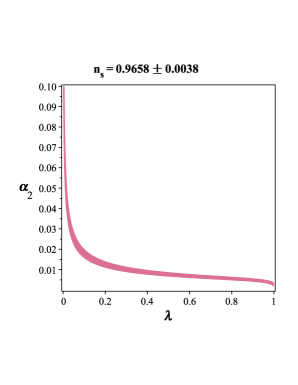
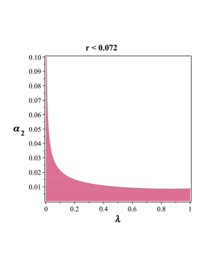
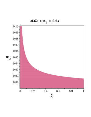
Figure 1: Ranges of the parameters $\alpha_{2}$ and $\lambda$ leading to the observationally viable values of the scalar spectral index (upper-left panel), tensor-to-scalar ratio (upper-right panel) and the tensor spectral index (lower panel) in the tachyon model with the superpotential.

4 Observational Viability

To study the observational viability of this model and find some constraints on the model’s parameters, we use the superpotential given in the equation (22). By this superpotential, we obtain slow-roll parameters (18)-(2.2) and therefore the perturbations parameters (scalar spectral index, tensor spectral index, and tensor-to-scalar ratio) in terms of the scalar fields and model’s parameters. Also, by using equations (15)-(17), we find the value of $\phi$ in terms of the e-folds number and model’s parameters and substitute it in the perturbations parameters. Now, we can compare the values of these parameters with observational data and obtain some constraints on the parameter $\alpha_{2}$ for some values of $\lambda$. As we have mentioned in the Introduction, from Planck2018 TT, TE, EE+lowE+lensing+BAO+BK14 data and by considering $\Lambda CDM+r+\frac{dn_{s}}{d\ln k}$ model, we have $n_{s}=0.9658\pm 0.0038$ at $68\%$ CL [34, 35]. By using this constraint, we have obtained the range of the parameters $\alpha_{2}$ and $\lambda$ leading to the observationally viable values of the scalar spectral index. The result is shown in the upper-left panel of figure 1. The upper-right panel of figure 1 shows the range of the parameters $\alpha_{2}$ and $\lambda$ which leads to $r<0.072$, obtained from Planck2018 TT, TE, EE+lowE+lensing+BAO+BK14 data at $68\%$ CL. Also, the lower panel of figure 1 shows the range of the parameters $\alpha_{2}$ and $\lambda$ leading to $-0.62<n_{T}<0.53$, obtained from Planck2018 TT, TE, EE +lowE+lensing+BK14+BAO+LIGO and Virgo2016 data at $68\%$ CL [34, 35]. To plot these figures, we have adopted $N=60$, $0<\alpha_{2}\leq 0.1$ and $0<\lambda\leq 1$.

To obtain some constraints on the model’s parameters space, we have plotted the evolution of the tensor-to-scalar ratio in the background of the Planck2018 TT, TE, EE+lowE+lensing+BAO+BK14 data. The result is shown in figure 2. As the figure shows, the tachyon inflation with superpotential in some ranges of the model’s parameter is consistent with observational data. We also have plotted the evolution of the tensor-to-scalar ratio versus the tensor spectral index in the background of the Planck2018 TT, TE, EE +lowE+lensing+BK14+BAO+LIGO and Virgo2016 data set in figure 3. Note that, as equation (35) and figure 3 show, the consistency relation in this setup is satisfied. By Using the numerical analysis, we have obtained some constraints on the parameter $\alpha_{2}$, for some sample values of $\lambda$ as $0.1$, $0.3$, $0.6$ and $0.9$, which have been summarized in table 1. Also, by using the constraints that Planck2018 TT, TE, EE+lowE+lensing+BAO+BK14 data at $68\%$ CL and $95\%$ CL set on the scalar spectral index and the tensor-to-scalar ratio, it is possible to obtain the ranges of the sound speed and $\lambda$ which fulfill the mentioned data. In this respect, figure 4 shows the observationally viable ranges of $\lambda$ and $c_{s}$ at $68\%$ CL (yellow region) and $95\%$ CL (magenta region).

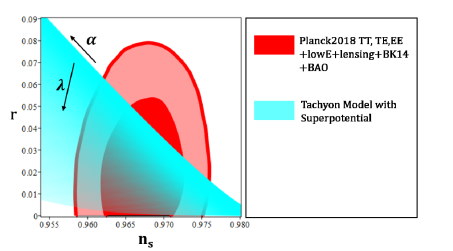
Figure 2: Tensor-to-scalar ratio versus the scalar spectral index in the tachyon model with superpotential. The arrows show the direction in which the parameters increase.

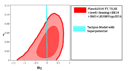
Figure 3: Tensor-to-scalar ratio versus the tensor spectral index in the tachyon model with superpotential.

Table 1: Ranges of the parameter $\alpha_{2}$ in which the tensor-to-scalar ratio, the scalar spectral index and the tensor spectral index of the tachyon inflation with superpotential are consistent with different data sets.

	Planck2018 TT,TE,EE+lowE	Planck2018 TT,TE,EE+lowE	Planck2018 TT,TE,EE+lowE	Planck2018 TT,TE,EE+lowE
	+lensing+BK14+BAO	+lensing+BK14+BAO	lensing+BK14+BAO	lensing+BK14+BAO
			+LIGO$\&$Virgo2016	LIGO$\&$Virgo2016
$\lambda$	$68\%$ CL	$95\%$ CL	$68\%$ CL	$95\%$ CL
$0.1$	$1.41\times 10^{-2}<\alpha_{2}<1.83\times 10^{-2}$	$1.11\times 10^{-2}<\alpha_{2}<1.98\times 10^{-2}$	$0.65\times 10^{-2}<\alpha_{2}<2.0.2\times 10^{-2}$	$0<\alpha_{2}<2.25\times 10^{-2}$
$0.4$	$0.68\times 10^{-2}<\alpha_{2}<0.91\times 10^{-2}$	$0.55\times 10^{-2}<\alpha_{2}<0.98\times 10^{-2}$	$0.35\times 10^{-2}<\alpha_{2}<1.03\times 10^{-2}$	$0<\alpha_{2}<1.15\times 10^{-2}$
$0.7$	$0.48\times 10^{-2}<\alpha_{2}<0.68\times 10^{-2}$	$0.39\times 10^{-2}<\alpha_{2}<0.73\times 10^{-2}$	$0.28\times 10^{-2}<\alpha_{2}<0.83\times 10^{-2}$	$0<\alpha_{2}<0.92\times 10^{-2}$
$0.9$	$0.17\times 10^{-2}<\alpha_{2}<0.55\times 10^{-2}$	$0.12\times 10^{-2}<\alpha_{2}<0.40\times 10^{-2}$	$0.43\times 10^{-2}<\alpha_{2}<0.84\times 10^{-2}$	$0<\alpha_{2}<0.90\times 10^{-2}$

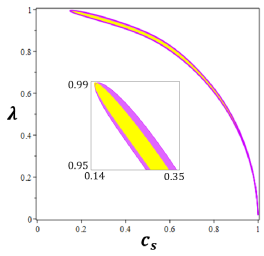
Figure 4: Ranges of the parameters $\lambda$ and $c_{s}$ leading to the observationally viable values of the scalar spectral index and the tensor-to-scalar ratio, obtained from Planck2018 TT, TE, EE+lowE+lensing+BAO+BK14 data at $68\%$ CL (yellow region) and $95\%$ CL (magenta region).

To study the non-gaussian feature of the primordial perturbations numerically, we consider equation (44) with the sound speed given in equation (21) and the superpotential (22). In fact, we seek for the prediction of the model about the amplitude of the non-gaussianity in the tachyon model with superpotential. In this regard, in figure 6 we have plotted the phase space of the parameters $\alpha_{2}$ and $\lambda$ and also the corresponding predicted values of the amplitude of the equilateral configuration of the non-gaussianity. As the figure shows, for most ranges of the parameter space, the tachyon model with superpotential predicts small non-gaussianity. In fact, if we consider $\lambda\leq 0.9$, for all values of $\alpha_{2}$, the amplitude of the equilateral non-gaussianity in the tachyon model is consistent with Planck2018 TTT, EEE, TTE and EET data at $68\%$ CL. However, if we consider $\lambda>0.9$, there would be some constraints on the parameter $\alpha_{2}$ in confrontation with Planck2018 TTT, EEE, TTE and EET data at $68\%$ CL. We have obtained some of these constraints which have been summarized in table 2. Also, from the constraints obtained by comparing the $r-n_{s}$ and $r-n_{T}$ behavior in the background of Planck2018 TT, TE, EE+lowE+lensing+BAO+BK14 data, it is possible to find the observationally viable values of the sound speed and the amplitude of the equilateral configuration of the non-gaussianity. The results of this numerical analysis have been summarized in table 3.

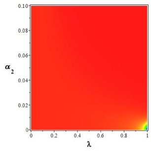
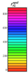
Figure 5: Space of the parameters $\alpha_{2}$ and $\lambda$ (left panel) and the corresponding predicted values of the amplitude of the equilateral non-gaussianity (right panel) in the tachyon model with superpotential.

Table 2: Ranges of the parameters $\alpha_{2}$ and $\lambda$ leading to the observationally viable values of the equilateral configuration of the non-gaussianity in the tachyon model with superpotential, in confrontation with the Planck2018 TTT, EEE, TTE and EET data at $68\%$ CL.

$0<\lambda\leq 0.9$	$\lambda=0.93$	$\lambda=0.96$	$\lambda=0.99$
$0<\alpha_{2}<0.1$	$0.004<\alpha_{2}<0.1$	$0.006<\alpha_{2}<0.1$	$0.008<\alpha_{2}<0.1$

Table 3: The observationally viable ranges of the sound speed and the amplitude of the equilateral configuration of the non-gaussianity in the tachyon inflation with superpotential, in confrontation with Planck2018 TT, TE, EE+lowE+lensing+BAO+BK14 data at $68\%$ CL.

$\lambda$		$c_{s}$		$f_{NL}^{equil}$
$0.1$		$0.994<c_{s}<0.995$		$0.039<f_{NL}^{equil}<0.040$
$0.4$		$0.920<c_{s}<0.923$		$0.727<f_{NL}^{equil}<0.759$
$0.7$		$0.727<c_{s}<0.740$		$3.47<f_{NL}^{equil}<3.74$
$0.9$		$0.464<c_{s}<0.493$		$13.0<f_{NL}^{equil}<15.2$

5 Reheating Phase after Inflation

After ending the inflationary expansion, the universe should be reheated for subsequent evolution. This process is named reheating phase of the universe which studying it gives us some more information about the model. In this regard, following [59, 60, 61, 62, 63], in this section we obtain some expressions for the e-folds number during the reheating, $N_{rh}$, (the subscript “$rh$” stands for the reheating) and temperature during this era, $T_{rh}$. Considering that these reheating parameters are expressed in terms of the scalar spectral index, it is possible to explore their observational viability.

We start with the following equation

$$N_{hc}=\ln\left(\frac{a_{e}}{a_{hc}}\right)\,,$$ (45)

defining the e-folds number between the time where physical scales cross the horizon and the time where the inflation epoch ends. By the subscript “$e$” we mean the end of inflation and by the subscript “$hc$” we show the horizon crossing. Note that, the relation $\rho\sim a^{-3(1+\omega_{eff})}$ for the energy density is satisfied during the reheating process. In this relation, the effective equation of state, corresponding to the dominant energy density of the universe, is shown by the parameter $\omega_{eff}$. By using this relation between the energy density and the equation of state parameter, we can find the e-folds number during reheating as follows

$$N_{rh}=\ln\left(\frac{a_{rh}}{a_{e}}\right)=-\frac{1}{3(1+\omega_{eff})}\ln\left(\frac{\rho_{rh}}{\rho_{e}}\right)\,.$$ (46)

On the other hand, at the horizon crossing of the physical scales we have

$$0=\ln\left(\frac{k_{hc}}{a_{hc}H_{hc}}\right)=\ln\left(\frac{a_{e}}{a_{hc}}\frac{a_{rh}}{a_{e}}\frac{a_{0}}{a_{rh}}\frac{k_{hc}}{a_{0}H_{hc}}\right)\,,$$ (47)

with subscript “$0$” being the current value of the corresponding parameter. Now, equations (45)-(47) give

$$N_{hc}+N_{rh}+\ln\left(\frac{k_{hc}}{a_{0}H_{hc}}\right)+\ln\left(\frac{a_{0}}{a_{rh}}\right)=0\,.$$ (48)

Now, we express $\frac{a_{0}}{a}$ in terms of the temperature and density. To this end, we use the following relation between the energy density and temperature during the reheating [61, 63]

$$\rho_{rh}=\frac{\pi^{2}g_{rh}}{30}T_{rh}^{4}\,.$$ (49)

In the above equation, the parameter $g_{rh}$ is the effective number of the relativistic species at the reheating era. Also, the conservation of the entropy gives the following equation [61, 63]

$$\frac{a_{0}}{a_{rh}}=\left(\frac{43}{11g_{rh}}\right)^{-\frac{1}{3}}\frac{T_{rh}}{T_{0}}\,.$$ (50)

From equations (49) and (50) we get

$$\frac{a_{0}}{a_{rh}}=\left(\frac{43}{11g_{rh}}\right)^{-\frac{1}{3}}T_{0}^{-1}\left(\frac{\pi^{2}g_{rh}}{30\rho_{rh}}\right)^{-\frac{1}{4}}\,.$$ (51)

In the tachyon model with superpotential, the energy density in terms of the slow-roll parameter $\epsilon$ is given by

$$\rho=\frac{\frac{\kappa^{2}}{6}W^{2}-\frac{1}{8}W^{\prime 2}}{\sqrt{1-\frac{2}{3}\epsilon}}\,.$$ (52)

At the end of inflation, where we have $\epsilon=1$, the energy density takes the following form

$$\rho_{e}=\sqrt{3}\,\bigg{(}\frac{\kappa^{2}}{6}W_{e}^{2}-\frac{1}{8}W_{e}^{\prime 2}\bigg{)}\,.$$ (53)

The energy density during the reheating era is obtained from equations (46) and (53) as follows

$$\rho_{rh}=\sqrt{3}\,\bigg{(}\frac{\kappa^{2}}{6}W_{e}^{2}-\frac{1}{8}W_{e}^{\prime 2}\bigg{)}\,\exp\Big{[}-3N_{rh}(1+\omega_{eff})\Big{]}.$$ (54)

Now, equations (51) and (53) give

$$\ln\left(\frac{a_{0}}{a_{rh}}\right)=-\frac{1}{3}\ln\left(\frac{43}{11g_{rh}}\right)-\frac{1}{4}\ln\left(\frac{\pi^{2}g_{rh}}{30\rho_{rh}}\right)-\ln T_{0}+\frac{1}{4}\ln\Bigg{(}\sqrt{3}\,\bigg{(}\frac{\kappa^{2}}{6}W_{e}^{2}-\frac{1}{8}W_{e}^{\prime 2}\bigg{)}\Bigg{)}$$

$$-\frac{3}{4}N_{rh}(1+\omega_{eff})\,.$$ (55)

By using equations (29), (48) and (5), we find the e-folds number during reheating as follows

$$N_{rh}=\frac{4}{1-3\omega_{eff}}\Bigg{[}-N_{hc}-\ln\Big{(}\frac{k_{hc}}{a_{0}T_{0}}\Big{)}-\frac{1}{4}\ln\Big{(}\frac{40}{\pi^{2}g_{rh}}\Big{)}-\frac{1}{3}\ln\Big{(}\frac{11g_{rh}}{43}\Big{)}$$

$$+\frac{1}{2}\ln\Big{(}8\pi^{2}{\cal{A}}_{s}{\cal{Q}}_{s}c_{s}^{3}\Big{)}-\frac{1}{4}\ln\Bigg{(}\sqrt{3}\,\bigg{(}\frac{\kappa^{2}}{6}W_{e}^{2}-\frac{1}{8}W_{e}^{\prime 2}\bigg{)}\Bigg{)}\Bigg{]}.$$ (56)

We can also find the temperature during reheating from equations (46), (50) and (53) as follows

$$T_{rh}=\bigg{(}\frac{30}{\pi^{2}g_{rh}}\bigg{)}^{\frac{1}{4}}\,\bigg{[}\sqrt{3}\,\bigg{(}\frac{\kappa^{2}}{6}W_{e}^{2}-\frac{1}{8}W_{e}^{\prime 2}\bigg{)}\bigg{]}^{\frac{1}{4}}\,\exp\bigg{[}-\frac{3}{4}N_{rh}(1+\omega_{eff})\bigg{]}\,.$$ (57)

Now, we study the reheating process numerically. To this end, by using equation (2), we obtain equations (5) and (57) in terms of the tachyon field $\phi$. After that, we use equations (18), (2.2), (2.2) and (31) to find the value of the tachyon field in terms of the scalar spectral index. In this way, we get the e-folds number and the temperature during the reheating phase in terms of $n_{s}$. By using the observational constraint on the scalar spectral index, obtained from Planck2018 TT, TE, EE+lowE+lensing+BK14+BAO joint data, we can find some constraints on $n_{rh}$ and $T_{rh}$. In this regard, in figure 6 we have plotted the e-fold number during reheating versus the effective equation of state. This figure has been plotted for some sample values of the parameters $\lambda$ and $\alpha_{2}$ which have been adopted from the constraints presented in table 1. Also, to plot this figure we have used the constraint on the scalar spectral index as $n_{s}=0.9658\pm 0.0038$. The range used for the effective equation of state is $-1\leq\omega_{eff}\leq 1$. In fact, at the end of the inflationary expansion, we have $\omega_{eff}=-\frac{1}{3}$ and at the beginning of the radiation dominated era $\omega_{eff}=\frac{1}{3}$. Therefore, the adopted range for the effective equation of state seems suitable for consideration. As the figure shows, the value of e-folds number during reheating increases by changing the value of the effective equation of state from $-1$ to $\frac{1}{3}$. Also, our numerical analysis shows that for $\lambda<0.2$ and $\alpha_{2}<1.53\times 10^{-2}$, it is possible to have instantaneous reheating. However, for $\lambda\geq 0.2$ and $\alpha_{2}\geq 1.53\times 10^{-2}$, a few e-folds number are needed for the reheating process to be completed. We have also plotted the behavior of $N_{rh}$ versus $n_{s}$, for some sample values of $\lambda$ and $\alpha_{2}$, in figure 7. In this figure, we have also adopted three values of the effective equation of state as $\omega_{eff}=-1,-\frac{1}{3}$ and $0$. The behavior of the temperature during the reheating versus the scalar spectral index is shown in figure 8. This figure has been plotted for the same values of the parameters as figure 7. By performing these numerical analyses, we have obtained some constraints on the important reheating parameters $N_{rh}$ and $T_{rh}$, summarized in tables 4 and 5.

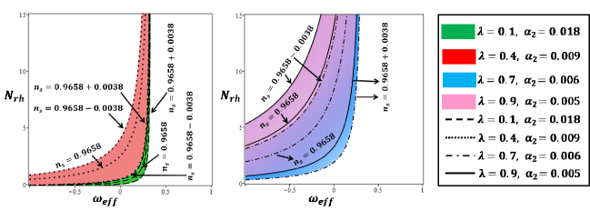
Figure 6: Ranges of the e-folds number and the effective equation of state parameter during the reheating phase for the tachyon model with superpotential, leading to the observationally viable values of the scalar spectral index.

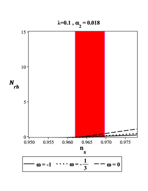
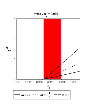
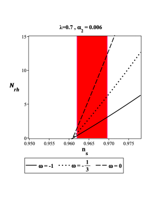
Figure 7: The behavior of the e-folds number during the reheating phase versus the scalar spectral index, for the tachyon model with superpotential. The red region shows the values of the scalar spectral index released by Planck2018 TT, TE, EE+lowE+lensing+BK14+BAO joint data at $68\%$ CL.

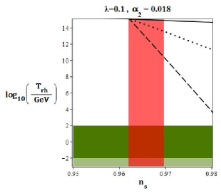
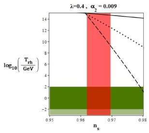
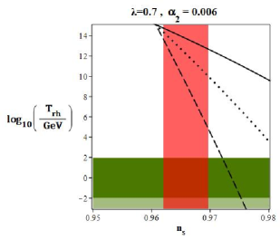
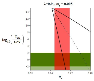
Figure 8: The behavior of the temperature during the reheating phase versus the scalar spectral index, for the tachyon model with superpotential. The dark green region shows the temperatures below the electroweak scale, $T<100$ GeV, and the light green region corresponds to the temperatures below the big bang nucleosynthesis scale, $T<10$ MeV.

Table 4: Constraints on the e-folds number during reheating in the tachyon model with superpotentail, obtained from Planck2018 TT, TE, EE+lowE+lensing+BK14+BAO joint data at $68\%$ CL.

$\lambda$	$\alpha_{2}$	$\omega=-1$	$\omega=-\frac{1}{3}$	$\omega=0$
$0.1$	$1.41\times 10^{-2}<\alpha_{2}<1.83\times 10^{-2}$	$0\leq N_{rh}\leq 0.134$	$0\leq N_{rh}\leq 0.181$	$0.012\leq N_{rh}\leq 0.513$
$0.4$	$0.68\times 10^{-2}<\alpha_{2}<0.91\times 10^{-2}$	$0.010\leq N_{rh}\leq 0.883$	$0.197\leq N_{rh}\leq 1.22$	$0.514\leq N_{rh}\leq 4.31$
$0.7$	$0.48\times 10^{-2}<\alpha_{2}<0.68\times 10^{-2}$	$0.201\leq N_{rh}\leq 3.32$	$0.862\leq N_{rh}\leq 6.67$	$1.72\leq N_{rh}\leq 15.6$
$0.9$	$0.17\times 10^{-2}<\alpha_{2}<0.33\times 10^{-2}$	$0.541\leq N_{rh}\leq 5.81$	$1.404\leq N_{rh}\leq 7.66$	$2.89\leq N_{rh}\leq 22.2$

Table 5: Constraints on the temperature during reheating in the tachyon model with superpotentail, obtained from Planck2018 TT, TE, EE+lowE+lensing+BK14+BAO joint data at $68\%$ CL.

$\lambda$	$\alpha_{2}$	$\omega=-1$	$\omega=-\frac{1}{3}$	$\omega=0$
$0.1$	$1.41\times 10^{-2}<\alpha_{2}<1.83\times 10^{-2}$	$14.6\leq\log_{10}\left(\frac{T_{rh}}{GeV}\right)$	$13.3\leq\log_{10}\left(\frac{T_{rh}}{GeV}\right)$	$9.91\leq\log_{10}\left(\frac{T_{rh}}{GeV}\right)$
$0.4$	$0.68\times 10^{-2}<\alpha_{2}<0.91\times 10^{-2}$	$14.3\leq\log_{10}\left(\frac{T_{rh}}{GeV}\right)\leq 14.9$	$12.2\leq\log_{10}\left(\frac{T_{rh}}{GeV}\right)\leq 14.6$	$8.69\leq\log_{10}\left(\frac{T_{rh}}{GeV}\right)\leq 14.2$
$0.7$	$0.48\times 10^{-2}<\alpha_{2}<0.68\times 10^{-2}$	$12.3\leq\log_{10}\left(\frac{T_{rh}}{GeV}\right)\leq 14.5$	$9.43\leq\log_{10}\left(\frac{T_{rh}}{GeV}\right)\leq 13.9$	$4.03\leq\log_{10}\left(\frac{T_{rh}}{GeV}\right)\leq 13.1$
$0.9$	$0.17\times 10^{-2}<\alpha_{2}<0.33\times 10^{-2}$	$11.5\leq\log_{10}\left(\frac{T_{rh}}{GeV}\right)\leq 14.3$	$6.32\leq\log_{10}\left(\frac{T_{rh}}{GeV}\right)\leq 12.9$	$\log_{10}\left(\frac{T_{rh}}{GeV}\right)\leq 10.8$

6 A Short Discussion on the Case with Quantum Effects

In this section, we study the consequence of presenting the quantum effects on the tachyon’s dynamics in the early universe. To this end, following Ref. [64], we include the quantum effect by considering the conformal anomaly. By considering ${\cal{N}}$ scalar, ${\cal{N}}_{1}$ vector fields, ${\cal{N}}_{2}$ gravitons, ${\cal{N}}_{\frac{1}{2}}$ spinor and ${\cal{N}}_{hd}$ higher-derivative conformal scalars, we have the anomalous trace of the stress tensor as [65, 66, 64]

$${\cal{T}}=b\left(\Upsilon+\frac{2}{3}\Box R\right)+b^{\prime}\,G\,,$$ (58)

wehere

$$b=\frac{{\cal{N}}+6{\cal{N}}_{\frac{1}{2}}+12{\cal{N}}_{1}+611{\cal{N}}_{2}-8{\cal{N}}_{hd}}{120(4\pi)^{2}}\,,$$ (59)

and

$$b^{\prime}=-\frac{{\cal{N}}+11{\cal{N}}_{\frac{1}{2}}+62{\cal{N}}_{1}+1411{\cal{N}}_{2}-28{\cal{N}}_{hd}}{360(4\pi)^{2}}\,.$$ (60)

If we consider a warped de-Sitter space-time with a scale factor as $a=e^{\frac{t}{L}}$ ($L$ is the curvature radius of the space-time), the energy density and pressure corresponding to the quantum effects are given by (see Refs. [66, 67])

$$\rho_{q}=-p_{q}=-\frac{6b^{\prime}}{L^{4}}\,.$$ (61)

Therefore, by considering the quantum effects and the tachyon field, the Friedmann equations (5) and (6) take the following forms

$$\frac{3}{L^{2}}=\frac{\kappa^{2}\,V(\phi)}{\sqrt{1-\lambda\,\dot{\phi}^{2}}}-\frac{6\kappa^{2}\,b^{\prime}}{L^{4}}\,,$$ (62)

$$\frac{3}{L^{2}}=\kappa^{2}\,V(\phi)\,\sqrt{1-\lambda\,\dot{\phi}^{2}}-\frac{6\kappa^{2}\,b^{\prime}}{L^{4}}\,.$$ (63)

Equations (62) and (63) are satisfied if $\dot{\phi}=0$ or $\phi=\phi_{0}=constant$. Also, from equation of motion (7) we find $V^{\prime}=0$. This means that in the presence of the quantum effects, the potential of the tachyon field becomes constant. We name this constant potential as $V_{0}$. Now, from equation (62) we have

$$\frac{1}{L^{2}}=-{\frac{1}{{4\,b^{\prime}}\,{\kappa}^{2}}}\pm\sqrt{{\frac{V_{0}}{6b^{\prime}}}+{\frac{1}{16\,{b^{\prime}}^{2}{\kappa}^{4}}}}\,.$$ (64)

Considering that $b^{\prime}$ is constant, equation (64) give us constant Hubble parameter. The constant Hubble parameter means $\epsilon=\eta=0$. Even we consider small potential (as the case in Ref. [64]) and consider the quantum effect as the running of inflation, there is still a problem. With a constant Hubble parameter, the inflation phase would never have a graceful exit. This problem remains even we assume the tachyon/phantom filed or a canonical scalar field. If we insist to account for the quantum effect in the inflation epoch, we may consider models with two scalar fields with quantum effects (as has been done in Ref. [64]) or maybe nonminimal coupling models.

7 Summary

In this paper, we have studied the tachyon inflation with the superpotential as an inflationary potential. In this regard, without including any supersymmetry, we have used a form of the potential which is similar to the one in the supergravity. By studying the inflation in this model, we have obtained the slow-roll parameters in terms of the superpotential. We have also explored the perturbations in this model at both the linear and non-linear levels. At the linear level, we have obtained the important perturbation parameters, such as the scalar spectral index, the tensor spectral index and the tensor-to-scalar ratio. At the non-linear level, we have obtained a parameter named non-linearity parameter which gives the amplitude of the non-gaussianity. Considering that the amplitude of the non-gaussianity in the tachyon model has a peak at the equilateral configuration, we have obtained the non-linearity parameter in this configuration.

After that, we have sought for the observational viability of the tachyon model with superpotential. In this regard, we have focused on the model’s parameters $\lambda$ and $\alpha_{2}$. By using the observational constraints on the perturbations parameters, obtained from Planck2018 TT, TE, EE+lowE+lensing+BAO+BK14 and Planck2018 TT, TE, EE +lowE+lensing+BK14+BAO+LIGO and Virgo2016 data at $68\%$ CL, we have obtained the observationally viable regions of the parameters $\lambda$ and $\alpha_{2}$. We have also studied the behavior of $r-n_{s}$ and $r-n_{T}$, in the background of Planck2018 TT, TE, EE+lowE+lensing+BAO+BK14 and Planck2018 TT, TE, EE +lowE+lensing+BK14+BAO+LIGO and Virgo2016 data, respectively, at $68\%$ CL and $95\%$ CL. Also, by using the observational constraints on the scalar spectral index at $68\%$ CL and $95\%$ CL, we have plotted the observationally viable ranges of the sound speed and $\lambda$ which fulfill the constraints. By these numerical analyses, we have obtained some constraints on the parameter $\alpha_{2}$ for some sample values of $\lambda$ as $\lambda=0.1,0.4,0.7$ and $0.9$. Our numerical analysis on the perturbations parameters shows that, depending on the values of $\lambda$, the tachyon model with superpotential is observationally viable if $0.040\times 10^{-2}\leq\alpha_{2}<0.1$ at $68\%$ CL and $0.021\times 10^{-2}\leq\alpha_{2}<0.1$ at $95\%$ CL. We have also studied the non-gaussian feature of the primordial perturbations numerically. By plotting the phase space of the parameters $\lambda$ and $\alpha_{2}$, we have presented the prediction of the tachyon model with superpotential for the amplitude of the equilateral non-gaussianity. We have shown that, for $\lambda>0.9$, to the amplitude of the primordial non-gaussianity be consistent with Planck2018 TTT, EEE, TTE and EET data, there are some constraints on the parameter $\alpha_{2}$. Note that, for $\lambda\leq 0.9$, all values of $\alpha_{2}$ lead to the observationally viable values of $f_{NL}^{equil}$.

Another issue that has been studied in this paper, is the reheating process after inflation by assuming the superpotential. To study this process, we have found the e-folds number and temperature during the reheating era in terms of the superpotential. Then, given the relation between these parameters and scalar spectral, by using the observational constraints on $n_{s}$, we have studied the parameters $N_{rh}$ and $T_{rh}$ numerically. We have shown that, by increasing the values of the e-folds number during the reheating phase, the effective equation of state in the tachyon model with superpotential increases from $-1$ to $\frac{1}{3}$ (corresponding to the radiation dominated universe). We have also, studied the behavior of the parameters $N_{rh}$ and $T_{rh}$ versus $n_{s}$ for some sample values of $\lambda$ and $\alpha_{2}$. Our numerical analysis shows that, in the tachyon model with superpotential, the reheating is instantaneous for $\lambda<0.2$ and $\alpha_{2}<1.53\times 10^{-2}$. In other cases, the reheating process needs a few e-folds number to be completed. We have also shortly discussed the case with presenting the quantum effects. It seems that if we consider the models with single scalar fields, the presence of quantum corrections makes the inflation phase permanent. To have a graceful exit from inflation, we may consider the quantum effects in two-field or nonminimal models.

Acknowledgement
I thank the referee for the very insightful comments that have improved the quality of the paper considerably.

References

• [1] A. Guth, Phys. Rev. D, 23, 347 (1981).
• [2] A. D. Linde, Physics Letters B 108, 389 (1982).
• [3] A. Albrecht & P. Steinhard, Phys. Rev. D 48, 1220 (1982).
• [4] A. D. Linde, Particle Physics and Inflationary Cosmology (Harwood Academic Publishers, Chur, Switzerland) (1990).
• [5] A. R. Liddle & D. Lyth, Cosmological Inflation and Large-Scale Structure, (Cambridge University Press) (2000).
• [6] J. E. Lidsey, A. R. Liddle, E. W. Kolb, E. J. Copeland, T. Barreiro & M. Abney, Rev. Mod. Phys. 69, 373 (1997).
• [7] A. Riotto, [arXiv:hep-ph/0210162] (2002).
• [8] D. H. Lyth & A. R. Liddle, The Primordial Density Perturbation (Cambridge University Press) (2009).
• [9] J. M. Maldacena, JHEP 0305, 013 (2003).
• [10] A. Sen, JHEP 10, 008 (1999).
• [11] A. Sen, JHEP 07, 065 (2002).
• [12] A. Sen, Modern Physics Letters A 17, 1797 (2002).
• [13] G.W. Gibbons, Phys. Lett. B 537, 1 (2002).
• [14] A. Feinstein, Phys. Rev. D 66, 063511 (2002).
• [15] S. del Campo, R. Herrera & A. Toloza, Phys. Rev. D 79, 083507 (2009).
• [16] K. Nozari & N. Rashidi, Phys. Rev. D 88, 023519 (2013).
• [17] N. Barbosa-Cendejas, J. De-Santiago, G. German, J. C. Hidalgo, R. R. Mora-Luna, JCAP 1511, 020 (2015).
• [18] K. Nozari & N. Rashidi, Phys. Rev. D 90, 043522 (2014).
• [19] Z. Bouabdallaoui, A. Errahmani, M. Bouhmadi-L$\acute{o}$pez & T. Ouali, Phys. Rev. D 94, 123508 (2016).
• [20] K. Rezazadeh, K. Karami, & S. Hashemi Phys. Rev. D 95, 103506 (2017).
• [21] N. Rashidi & K. Nozari, IJMPD 27, 1850076 (2018).
• [22] N. Bartolo, E. Komatsu, S. Matarrese & A. Riotto, 2004 Phys. Rept. 402, 103.
• [23] X. Chen, 2010, Adv. Astron., 2010, 638979.
• [24] A. De Felice, & S. Tsujikawa, JCAP, 1104, 029 (2011).
• [25] A. De Felice & S. Tsujikawa, Phys. Rev. D 84, 083504 (2011).
• [26] K. Nozari & N. Rashidi, Advances in High Energy Physics 2016, Article ID 1252689 (2015).
• [27] K. Nozari & N. Rashidi, Phys. Rev. D 93, 124022 (2016).
• [28] K. Nozari & N. Rashidi, Phys. Rev. D 95, 123518 (2017).
• [29] K. Nozari & N. Rashidi, The Astrophysical Journal, 863, 133 (2018).
• [30] S. Nojiri, S. D. Odintsov, V. K. Oikonomou & N. Chatzarakis, Eur. Phys. J. C, 79, 565 (2019).
• [31] N. Rashidi & K. Nozari, Phys. Rev. D, 102, 123548 (2020)
• [32] K. Nozari & N. Rashidi, The Astrophysical Journal, 863, 133 (2019).
• [33] N. Rashidi & K. Nozari The Astrophysical Journal, 890, 55 (2020).
• [34] N. Aghanim, Y. Akrami, M. Ashdown, J. Aumont, C. Baccigalupi, et al. [arXiv:1807.06209] (2018).
• [35] Y. Akrami, F. Arroja, M. Ashdown, J. Aumont, C. Baccigalupi, et al. [arXiv:1807.06211] (2018).
• [36] Y. Akrami, F. Arroja, M. Ashdown, J. Aumont, C. Baccigalupi, et al., [arXiv:1905.05697] (2019).
• [37] L. F. Abbott, E. Farhi, and M. B. Wise, Phys. Lett. B 117, 29 (1982).
• [38] A. D. Dolgov and A. D. Linde, Phys. Lett. B 116, 329 (1982).
• [39] A. J. Albrecht, P. J. Steinhardt, M. S. Turner and F. Wilczek, Phys. Rev. Lett. 48, 1437 (1982).
• [40] L. Kofman, A. D. Linde, & A. A. Starobinsky, Phys. Rev. Lett. 73, 3195 (1994).
• [41] L. Kofman, A. D. Linde, & A. A. Starobinsky, Phys. Rev. D 56, 3258 (1997).
• [42] G. F. Giudice, I. Tkachev & A. Riotto, JHEP 9908, 009 1999.
• [43] B. Wallisch Cosmological Probes of Light Relics, (PhD Thesis), [arXiv:1810.02800 [astro-ph.CO]] (2018).
• [44] M. Dine & A. Kusenko Rev. Mod. Phys, 76, 1 (2004).
• [45] K. D. Lozanov & M. A. Amin Phys. Rev. D, 90, 083528 (2014).
• [46] M. A. Amin, M. P. Hertzberg, D. I. Kaiser and J. Karouby , Int. J. Mod. Phys. D 24, 1530003 (2015).
• [47] K. Behrndt and M. Cvetic, Phys. Lett. B 475, 253 (2000).
• [48] O. DeWolfe, D. Z. Freedman, S. S. Gubser and A. Karch, Phys. Rev. D 62, 046008 (2000).
• [49] C. Csaki, J. Erlich, C. Grojean and T. Hollowood, Nucl. Phys. B 584, 359 (2000).
• [50] S. C. Davis, J. High Energy Phys. 0203, 054 (2002).
• [51] K. Nozari, M. Khamesian and N. Rashidi, Astropart. Phys. 35, 828 (2012).
• [52] K. Nozari and N. Rashidi, Astrophys. Space Sci. 347, 375 (2013).
• [53] V. F. Mukhanov, H. A. Feldman & R. H. Brandenberger, Physics Reports 215, 203 (1992).
• [54] C. Cheung, P. Creminelli, A. L. Fitzpatrick, J. Kaplan & L. Senatore, JHEP 03, 014 (2008).
• [55] X. Chen, M. -X. Huang, S. Kachru & G. Shiu, JCAP 0701, 002 (2007).
• [56] D. Babich, P. Creminelli & M. Zaldarriaga, JCAP 0408 09 (2004).
• [57] A. De Felice & S. Tsujikawa, JCAP 03, 030 (2011).
• [58] D. Baumann, [arXiv:0907.5424] (2012).
• [59] L. Dai, M. Kamionkowski and J. Wang, Phys. Rev. Lett. 113, 041302 (2014).
• [60] J. B. Munoz and M. Kamionkowski, Phys. Rev. D 91, 043521 (2015).
• [61] J. L. Cook, E. Dimastrogiovanni, D. Easson and L. M. Krauss, JCAP 04, 047 (2015).
• [62] R.-G. Cai, Z.-K. Guo and S.-J. Wang, Phys. Rev. D 92, 063506 (2015).
• [63] Y. Ueno and K. Yamamoto, Phys. Rev. D 93, 083524 (2016).
• [64] S. Nojiri & S. D. Odintsov, Phys. Lett. B, 571, 1-10 (2003).
• [65] M. J. Duff, Nucl. Phys. B, 125, 334 (1977).
• [66] S. Nojiri & S. D. Odintsov, Int. J. Mod. Phys. A 16, 3273 (2001).
• [67] S. Nojiri & S. D. Odintsov, Int. J. Mod. Phys. A 17, 4809 (2002).