Cardinality Minimization, Constraints, and Regularization: A Survey

Abstract

We survey optimization problems that involve the cardinality of variable vectors in constraints or the objective function. We provide a unified viewpoint on the general problem classes and models, and give concrete examples from diverse application fields such as signal and image processing, portfolio selection, or machine learning. The paper discusses general-purpose modeling techniques and broadly applicable as well as problem-specific exact and heuristic solution approaches. While our perspective is that of mathematical optimization, a main goal of this work is to reach out to and build bridges between the different communities in which cardinality optimization problems are frequently encountered. In particular, we highlight that modern mixed-integer programming, which is often regarded as impractical due to commonly unsatisfactory behavior of black-box solvers applied to generic problem formulations, can in fact produce provably high-quality or even optimal solutions for cardinality optimization problems, even in large-scale real-world settings. Achieving such performance typically draws on the merits of problem-specific knowledge that may stem from different fields of application and, e.g., shed light on structural properties of a model or its solutions, or lead to the development of efficient heuristics; we also provide some illustrative examples.

90-02, 90C05, 90C06, 90C10, 90C11, 90C26, 90C30, 90C33, 90C59, 90C90, 62J07, 68T99, 94A12, 91G10

1 Introduction

The cardinality of variable vectors occurs in a plethora of optimization problems, in either constraints or the objective function. In the following, we attempt to describe the broad landscape of such problems with a general emphasis on continuous variables. This restriction serves as a natural distinguishing feature from a myriad of classical operations research or combinatorial optimization problems, where “cardinality” typically appears in the form of minimizing or limiting the number of some objects associated with (non-auxiliary, i.e., structural) binary decision variables. Cardinality restrictions on general variables are thus of a decidedly different flavor, and also require different modeling and solution techniques than those immediately available in the binary case.

The general classes of problems we are interested in can be formalized as follows:

• Cardinality Minimization Problems

  ($$\ell_{0} X \min\leavevmode\nobreak\ \lVert{x}\rVert_{0}\quad\text{s.t.}\quad x\in X\subset{\mathds{R}}^{n},$$-min())

• Cardinality-Constrained Problems

  ($$\ell_{0} f k X \min\leavevmode\nobreak\ f(x)\quad\text{s.t.}\quad\lVert{x}\rVert_{0}\leq k,\quad x\in X\subseteq\mathds{R}^{n},$$-cons(, , ))

• Regularized Cardinality Problems

  ($$\ell_{0} \rho X \min\leavevmode\nobreak\ \lVert{x}\rVert_{0}+\rho(x)\quad\text{s.t.}\quad x\in X\subseteq\mathds{R}^{n},$$-reg(, ))

where we use $\lVert{x}\rVert_{0}\coloneqq\lvert{\operatorname{supp}(x)}\rvert=\lvert{\{j:x_{j}\neq 0\}}\rvert$ (the so-called “$\ell_{0}$-norm”), $f:\mathds{R}^{n}\to\mathds{R}$, $k\in\mathds{N}$, and $\rho:\mathds{R}^{n}\to\mathds{R}_{+}$. The set $X$ in any of these problems can be used to impose further constraints on $x$. For simplicity, we will usually simply write out the constraints rather than fully state the corresponding set $X$; e.g., we may write $\ell_{0}$-cons($f$, $k$, $g(x)\leq 0$) instead of $\ell_{0}$-cons($f$, $k$, $\{x\in\mathds{R}^{n}:g(x)\leq 0\}$).

Most concrete problems we will discuss belong to one of these three classes, although we will also encounter variations and extensions. Indeed, very similar problems may arise in very different fields of application, sometimes resulting in some methodology being reinvented or researchers being generally unaware of relevant results and developments from seemingly disparate communities. Moreover, the incomplete transfer of knowledge between different disciplines may prevent progress in the resolution of some problems that could strongly benefit of new approaches for similar problems, developed with completely different applications in mind. With this document, we hope to provide a useful roadmap connecting several disciplines and offering an overview of the many different computational approaches that are available for cardinality optimization problems. Note that a similar overview was given a couple of years ago in [351], but with a much more limited scope of cardinality problems and their aspects than we consider here (albeit discussing the related case of semi-continuous variables in more detail, in particular associated perspective reformulations, which we mostly skip). Moreover, significant advances have been achieved in just these past few years, which we include in this survey.

To emphasize the cross-disciplinary nature of many of the cardinality optimization problem classes and to provide a clear reference point for members of different communities to recognize their own problem of interest in this survey, we will group our overview of various concrete such problems according to the respective application areas and point out overlaps and differences. The solution methods we shall discuss cover both exact and heuristic approaches; our own mathematical programming perspective tends to favor exact models and algorithms that can provide provable guarantees on solution quality, a stance that appears to be less commonly taken in practical applications. This is “a feature, not a bug” of the present paper—we hope to bring across that in many cases, mixed-integer programming (MIP) offers an attractive alternative to widely-used heuristic methods. Generally, a typical first step in that direction is experimenting with off-the-shelf solvers to tackle basic MIP formulations. Depending on the application, this may already work very well, especially when solution quality is more important than speed. Importantly, MIP solvers also provide certifiable error bounds of the computed solution w.r.t. the optimum if terminated prematurely (e.g., when imposing a runtime limit), in contrast to many heuristic methods without general quality guarantees that are commonly employed in various applications. Moreover, improvement to optimality is often not hopeless and can be achieved either by simply allowing more solving time, or by improving the underlying mathematical model formulation and/or incorporating knowledge of the problem at hand into the MIP solver. Thus, as subsequent steps to substantially improve speed and scalability of MIP approaches, it is worth revisiting the model and guiding or enhancing the MIP solver by customizing existing (and/or adding new problem-specific) algorithmic components—a fact we will document with some examples.

We organize the subsequent discussion as follows: In the remainder of this introductory section, we will clarify some relationships between the main problem classes and fix our notation. Then, in Section 2, we describe the most common different realizations of the above problems $\ell_{0}$-min($X$), $\ell_{0}$-cons($f$, $k$, $X$), and $\ell_{0}$-reg($\rho$, $X$) as they occur in diverse fields like signal processing, compressed sensing, portfolio optimization, and machine learning; some further related problems are also discussed. In Section 3, we summarize exact modeling techniques (in particular, mixed-integer linear and nonlinear programming) and algorithmic approaches from the literature, and provide some exemplary numerical experiments to illustrate how the sometimes unsatisfactory performance of general-purpose models and MIP solvers may be significantly improved by some advanced modeling tricks and, especially, by integrating problem-specific knowledge and heuristic methods. This is followed in Section 4 by reviewing the plethora of proposed relaxations, regularization, and heuristic schemes, including popular $\ell_{1}$-norm and atomic norm minimization as well as greedy methods. Finally, in Section 5, we address scalability aspects of exact and approximate/heuristic algorithms, and then conclude the paper in Section 6.

Moreover, Table 1 provides an alternative overview meant to facilitate navigating this document if one is primarily interested in one specific problem. Since this paper covers too many different problems to provide such an overview for all of them, we do so exemplarily for three of the most-widely used problems, and note that the pointers to topics and locations given for these should also be helpful for many other related problems as well. Specifically, Table 1 covers $\ell_{0}$-min($\lVert{Ax-b}\rVert_{2}\leq\delta$), $\ell_{0}$-cons($\lVert{Ax-b}\rVert_{2}$, $k$, $\mathds{R}^{n}$), and $\ell_{0}$-reg($\tfrac{1}{2\lambda}\lVert{Ax-b}\rVert_{2}^{2}$, $\mathds{R}^{n}$), which will be formally introduced first in Section 2.1 in the context of signal processing, but also appear in virtually all other application areas, and can be seen as the “base problems” for various related variants and extensions.

Table 1: Some pointers to locations in this survey where information for the exemplary problems $\ell_{0}$-min($\lVert{Ax-b}\rVert_{2}\leq\delta$), $\ell_{0}$-cons($\lVert{Ax-b}\rVert_{2}$, $k$, $\mathds{R}^{n}$), and $\ell_{0}$-reg($\tfrac{1}{2\lambda}\lVert{Ax-b}\rVert_{2}^{2}$, $\mathds{R}^{n}$) can be found. Section 3.1 provides several reformulations of cardinality that are applicable to all problems; scalability of algorithms is discussed in Section 5.  

problem	location	information
$\ell_{0}$-min($\lVert{Ax-b}\rVert_{2}\leq\delta$)	Sect. 3.2	exact solution methods, mostly based on mixed-integer programming
	Sect. 4.1	$\ell_{1}$-surrogate problem BPDN($\delta,\mathds{R}^{n}$) and solution approaches, e.g., homotopy methods, ADMM, and smoothing techniques
	Sect. 4.3	heuristics based on nonconvex approximations (but only considering related constraints)
	Sect. 4.5	other heuristics such as subspace pursuit
$\ell_{0}$-cons($\lVert{Ax-b}\rVert_{2}$, $k$, $\mathds{R}^{n}$)	Sect. 3.3	exact solution methods, mostly based on mixed-integer programming
	Sect. 4.1	$\ell_{1}$-surrogate problem LASSO($\tau,\mathds{R}^{n}$) and solution approaches, e.g., a spectral projected gradient method and smoothing techniques
	Sect. 4.4	heuristics based on nonconvex formulations
	Sect. 4.5	other heuristics such as iterative hard-thresholding and matching pursuit
$\ell_{0}$-reg($\tfrac{1}{2\lambda}\lVert{Ax-b}\rVert_{2}^{2}$, $\mathds{R}^{n}$)	Sect. 3.4	theoretical discussion of the general problem $\ell_{0}$-reg($\rho$, $X$), some exact solution methods for special cases, possibilities for $\ell_{0}$-reg($\tfrac{1}{2\lambda}\lVert{Ax-b}\rVert_{2}^{2}$, $\mathds{R}^{n}$)
	Sect. 4.1	$\ell_{1}$-surrogate problem $\ell_{1}$-LS($\lambda,\mathds{R}^{n}$) and solution approaches, e.g., iterative soft-thresholding and semismooth Newton methods
	Sect. 4.4	heuristics based on nonconvex reformulations
	Sect. 4.5	other heuristics such as iterative hard-thresholding

1.1 Relationships Between Main Problem Classes

At least in some communities, it appears to be folklore knowledge that problems belonging to the classes $\ell_{0}$-min($X$), $\ell_{0}$-cons($f$, $k$, $X$), or $\ell_{0}$-reg($\rho$, $X$) can sometimes be equivalent in the sense that they share optimal solutions under certain assumptions on the cardinality, constraint and regularization parameters. Indeed, the fact that in widely-used surrogate models like $\ell_{1}$-norm problems, such equivalences always hold for the right parameter choices (cf. Section 4.1), might mislead one to presume the same is true for the $\ell_{0}$-based problems. However, this is generally not the case. We formalize (non-)equivalence statements for the three main classes of cardinality problems in the following result, where we let $\mbox{$\ell_{0}$-{min}({$\delta$})}\coloneqq\min\{\lVert{x}\rVert_{0}\,:\,f(x)\leq\delta,\leavevmode\nobreak\ x\in X\}$ be the typical slight variation of the cardinality minimization problem that most naturally relates to the other problem classes; to simplify notation, we also abbreviate $\ell_{0}$-cons$(k)\coloneqq\mbox{$\ell_{0}$-{cons}({$f$},\,{$k$},\,{$X$})}$, and $\ell_{0}$-reg$(\lambda)\coloneqq\mbox{$\ell_{0}$-{reg}({$\tfrac{1}{\lambda}f$},\,{$X$})}$.

Proposition 1.

Let $\lambda>0$, $\delta\geq 0$, $X\subseteq\mathds{R}^{n}$, and $f:\mathds{R}^{n}\to\mathds{R}$.

1. If $x^{*}$ is an optimal solution of $\ell_{0}$-reg$(\lambda)$, then it also optimally solves $\ell_{0}$-cons$(k)$ for $k=\lVert{x^{*}}\rVert_{0}$ and $\ell_{0}$-min($\delta$) for $\delta=f(x^{*})$. The reverse implications are not true in general.

2. If all optimal solutions $x^{*}$ of $\ell_{0}$-cons$(k)$ have the same cardinality $\lVert{x^{*}}\rVert_{0}$, then they all also solve $\ell_{0}$-min($\delta$) for $\delta=f(x^{*})$. The equal-cardinality assumption cannot be dropped in general.

3. If all optimal solutions $x^{*}$ of $\ell_{0}$-min($\delta$) have the same function value $f(x^{*})$, then they all also solve $\ell_{0}$-cons$(k)$ for $k=\lVert{x^{*}}\rVert_{0}$. The equal-value assumption cannot be dropped in general.

Proof 1.1.

First, let $x^{*}$ solve $\ell_{0}$-reg$(\lambda)$. Then, for all $x\in X$ with $\lVert{x}\rVert_{0}\leq k=\lVert{x^{*}}\rVert_{0}$, it holds that $f(x^{*})=f(x^{*})+\lambda(\lVert{x^{*}}\rVert_{0}-k)\leq f(x)+\lambda(\lVert{x}\rVert_{0}-k)\leq f(x)$, and for all $x\in X$ with $f(x)\leq\delta=f(x^{*})$, we have $\lVert{x^{*}}\rVert_{0}=\lVert{x^{*}}\rVert_{0}+\tfrac{1}{\lambda}(f(x^{*})-\delta)\leq\lVert{x}\rVert_{0}+\tfrac{1}{\lambda}(f(x)-\delta)\leq\lVert{x}\rVert_{0},$ which shows that $x^{*}$ solves both $\ell_{0}$-cons$(\lVert{x^{*}}\rVert_{0})$ and $\ell_{0}$-min($f(x^{*})$) as claimed. To show that the reverse implications do not hold in general, consider the case $X=\mathds{R}^{2}$ and $f(x)=\lVert{Ax-b}\rVert_{2}^{2}$ with

$$A=\begin{pmatrix}0&1\\ 1&2\end{pmatrix}\quad\text{and}\quad b=\begin{pmatrix}1\\ 0\end{pmatrix}.$$

Then, in particular, $\hat{x}_{1}=(0,\tfrac{1}{5})^{\top}$ optimally solves both $\ell_{0}$-cons$(1)$ and $\ell_{0}$-min($\tfrac{4}{5}$); $\ell_{0}$-cons$(0)$ is solved by $\hat{x}_{0}=(0,0)^{\top}$ with $f(\hat{x}_{0})=1$ and $\ell_{0}$-cons$(2)$ by $\hat{x}_{2}=(-2,1)^{\top}$ with $f(\hat{x}_{2})=0$. Thus, the optimal value of $\ell_{0}$-reg$(\lambda)$ as a function of $\lambda>0$ is

$$\min\big{\{}\tfrac{0}{\lambda}+2,\tfrac{4}{5\lambda}+1,\tfrac{1}{\lambda}+0\big{\}}=\begin{cases}2,&\lambda\in(0,\tfrac{1}{2}],\\ \tfrac{1}{\lambda},&\lambda\in[\tfrac{1}{2},\infty).\end{cases}$$

For $\lambda\in(0,\tfrac{1}{2})$, the solution to $\ell_{0}$-reg$(\lambda)$ is $\hat{x}_{2}$, for $\lambda=\tfrac{1}{2}$, both $\hat{x}_{0}$ and $\hat{x}_{2}$ are optimal, and for $\lambda>\tfrac{1}{2}$, only $\hat{x}_{0}$ is. This means that $\hat{x}_{1}$ cannot by recovered by $\ell_{0}$-reg$(\lambda)$ for any $\lambda>0$, which concludes the proof of statement 1.

We skip the straightforward proofs of the positive statements in 2 and 3. To show that these implications are not true without the respective assumptions, let $X=\mathds{R}^{2}$ and first consider $f(x)=x_{1}^{2}$. Then, any $x^{*}=(0,c)^{\top}$ with $c\in\mathds{R}$ optimally solves $\ell_{0}$-cons$(1)$, but not $\ell_{0}$-min($0$) unless $c=0$. Now, let $f(x)=(x_{1}-2)^{2}$. Then, $\hat{x}_{1}=(1,0)^{\top}$ and $\hat{x}_{2}=(2,0)^{\top}$ are both optimal for $\ell_{0}$-min($1$), but $\hat{x}_{1}$ does not solve $\ell_{0}$-cons$(1)$.

Note that points 2 and 3 of Proposition 1 imply equivalence of $\ell_{0}$-cons$(k)$ and $\ell_{0}$-min($\delta$), for the appropriate values of $k$ and $\delta$, in case of solution uniqueness, which is often an important desideratum (e.g., for signal reconstruction). However, the parameter values that yield such an equivalence are typically not known a priori.

1.2 Notation

We let $\mathds{R}_{+}$ denote the set of nonnegative real numbers. For a natural number $n\in\mathds{N}$, we abbreviate $[n]\coloneqq\{1,2,\dots,n\}$. The complement of a set $S\subset T$ is denoted by $S^{c}$. The cardinality of a vector $x$ is denoted as $\lVert{x}\rVert_{0}\coloneqq\lvert{\operatorname{supp}(x)}\rvert=\lvert{\{i:x_{i}\neq 0\}}\rvert$, where $\operatorname{supp}(x)$ is its support (i.e., index set of nonzero entries). The standard $\ell_{p}$-norm (for $1\leq p<\infty$) of a vector $x\in\mathds{R}^{n}$ is defined as $\lVert{x}\rVert_{p}\coloneqq(\sum_{i=1}^{n}|x_{i}|^{p})^{1/p}$, and $\lVert{x}\rVert_{\infty}\coloneqq\max|x_{i}|$. For a matrix $A$, $\lVert{A}\rVert_{\text{F}}$ denotes is Frobenius norm, and $A_{i}$ its $i$-th column. For a set $S$ and a vector $x$ or matrix $A$, $x_{S}$ and $A_{S}$ denote the vector restricted to indices in $S$ or the column-submatrix induced by $S$, respectively. We use $\mathds{1}$ to denote an all-ones vector, and $I$ to denote the identity matrix, of appropriate dimensions. A superscript $\top$ denotes transposition (of a vector or matrix). A diagonal matrix build from a vector $z$ is denoted by $\operatorname{Diag}(z)$, and conversely, $\operatorname{diag}(Z)$ extracts the diagonal of a matrix $Z$ as a vector. For vectors $\ell,u\in\mathds{R}^{n}$, we sometimes abbreviate $\ell\leq x\leq u$ (i.e., $\ell_{i}\leq x_{i}\leq u_{i}$ for all $i\in[n]$) as $x\in[\ell,u]$, extending the standard interval notation to vectors.

2 Prominent Cardinality Optimization Problems

Fig. 1: An overview of broader application areas and exemplary problems therein that share significant interests in cardinality optimization. Overlaps of concrete problem types across fields are quite common; for instance, cardinality-constrained Markowitz portfolio selection can be rewritten in the form of a constrained sparse regression problem (cf. [52]), which in turn is of the same class as certain signal denoising/reconstruction models, see Sections 2.1–2.3 for details.

Cardinality optimization problems (COPs, for short) abound in several different areas of application, such as medical imaging (e.g., X-ray tomography), face recognition, wireless sensor network design, stock-picking, crystallography, astronomy, computer vision, classification and regression, interpretable machine learning, or statistical data analysis, to name but a few. In this section, we highlight the most prominent realizations of such problems. To facilitate “mapping” concrete problems to concrete applications, we structure the section according to the three broad fields in which cardinality optimization problems are encountered most frequently: signal and image processing, portfolio optimization and management, and high-dimensional statistics and machine learning; further related COPs and extensions are gathered in a final subsection. Along these lines, a first broad overview of applications is provided in Figure 1.

2.1 Signal and Image Processing

In the broad field of signal processing, it has been found that signal sparsity can be exploited beneficially in several tasks, e.g., to remove noise from image or audio data or to reduce the amount of measurements needed to faithfully reconstruct signals from observations. In particular, the advent of compressed sensing (see [184] for a thorough introduction) has sparked a tremendous interest in several core cardinality optimization problems in the past 15 years or so.

At first, the focus was on reconstruction from linear measurements ($b=Ax$), but research quickly also expanded to different nonlinear settings. We will discuss the respective fundamental sparse recovery tasks in Sections 2.1.1 and 2.1.2 below; Section 2.1.3 covers important generalizations of the main sparsity concept.

Before we get started, a brief remark on the measurement matrices $A$ seems in order: In signal processing applications, $A$ is typically not fully generic but assumes certain forms and properties arising from an underlying physical measurement model or setup. Also, much of the theory for efficient solvability (see, e.g., Section 4.1.1) relies on properties of $A$ that hold with high probability for certain random matrices. Thus, in signal processing and, in particular, compressed sensing, one often encounters matrices such as Fourier transforms, Gaussian or Bernoulli matrices—sometimes combined with binary masks to blot out random entries, or otherwise modified. In contrast, we note that in other areas of application for the problems introduced in the following (or related tasks), the matrix $A$ is often comprised of observational data (e.g., in finance, regression or machine learning), which is typically unstructured and rarely beholden to specific probability distributions. This distinction may be partially responsible for the many different approaches found across disciplines.

2.1.1 Sparse Recovery From Linear Measurements

The fundamental sparse recovery problem takes the form

($$\ell_{0} Ax=b \min\leavevmode\nobreak\ \lVert{x}\rVert_{0}\quad\text{s.t.}\quad Ax=b,$$-min())

where $A\in\mathds{R}^{m\times n}$ with (w.l.o.g.) $\operatorname{rank}(A)=m<n$, and $b\in\mathds{R}^{m}$. Its variant allowing for noise in the linear measurements is usually deemed more realistic (although real-world applications for the above noise-free setting do exist) and can be formulated as

($$\ell_{0} \lVert{Ax-b}\rVert_{2}\leq\delta \min\leavevmode\nobreak\ \lVert{x}\rVert_{0}\quad\text{s.t.}\quad\lVert{Ax-b}\rVert_{2}\leq\delta,$$-min())

with some $\delta\in(0,\lVert{b}\rVert_{2})$ that is often derived from statistical properties of the noise in applications. The assumption $\delta<\lVert{b}\rVert_{2}$ excludes the otherwise trivial all-zero solution. Depending on noise models and application contexts, the $\ell_{2}$-norm in the constraint may be replaced by the $\ell_{1}$-norm (e.g., when the noise is impulsive, cf. [168]), by the $\ell_{\infty}$-norm (in case of uniform quantization noise or for sparse linear discriminant analysis, cf. [80, 89], respectively), or possibly by general $\ell_{p}$-(quasi-)norms for some $p>0$.

An alternative to cardinality minimization seeks to optimize data fidelity within a prescribed sparsity level $k\in\mathds{N}$ of the signal vector to be reconstructed, i.e., typically,

($$\ell_{0} \lVert{Ax-b}\rVert_{2} k \mathds{R}^{n} \min\leavevmode\nobreak\ \lVert{Ax-b}\rVert_{2}\quad\text{s.t.}\quad\lVert{x}\rVert_{0}\leq k.$$-cons(, , ))

This problem is often also referred to as subset selection or feature selection, see, e.g., [292, 55], and plays an important role in many regression and machine learning tasks (see also Section 2.3). Here, as for $\ell_{0}$-min($\lVert{Ax-b}\rVert_{2}\leq\delta$), the $\ell_{2}$-norm term is often rewritten equivalently as $\tfrac{1}{2}\lVert{Ax-b}\rVert_{2}^{2}$ to ensure differentiability (in $x$ with $Ax=b$) and simplify derivative notation; variants employing other norms also exist. The special case with orthogonal $A$ yields a sparse version of the standard denoising problem, where one seeks to “clean up” a noisy version $b=x+e$ of the target signal $x$ (in case $A=I$, cf. [165]), often incorporating an orthogonal basis transformation ($A\neq I$ but orthogonal, as in, e.g., [154, 153, 279]). Going beyond orthogonal bases, i.e., utilizing sparse representability w.r.t. more general $A$—such as overcomplete dictionaries, see Section 2.1.3 below—can further improve denoising capabilities, e.g., in image processing, see, for instance, [165] and references therein.

By its respective definition, $\ell_{0}$-min($\lVert{Ax-b}\rVert_{2}\leq\delta$) requires (approximate) knowledge of the noise level $\delta$, and for $\ell_{0}$-cons($\lVert{Ax-b}\rVert_{2}$, $k$, $\mathds{R}^{n}$), the user must specify the allowed sparsity level $k$. Since in practice it may be unclear how to choose either $\delta$ or $k$ appropriately, the regularization approach

($$\ell_{0} \tfrac{1}{2\lambda}\lVert{Ax-b}\rVert_{2}^{2} \mathds{R}^{n} \min\leavevmode\nobreak\ \lVert{x}\rVert_{0}+\tfrac{1}{2\lambda}\lVert{Ax-b}\rVert_{2}^{2}$$-reg(, ))

has also been thoroughly investigated. Note that this problem is also particularly suitable to situations where the noise has limited variance (but its level is unknown), and a sparse solution (of unknown cardinality) is sought. Here, the regularization parameter $\lambda>0$ controls the tradeoff between sparsity of the solution and data fidelity. While this model has the potential advantage of being unconstrained, it is similarly unclear how to “correctly” choose $\lambda$ in most applications. In general, there are many different approaches to obtain regularization, sparsity or residual error-bound parameters that work well for an application at hand, including homotopy schemes and cross-validation techniques.

A fundamental question from the signal processing perspective is that of uniqueness of the recovery problem solution. In particular, for the basic reconstruction problem $\ell_{0}$-min($Ax=b$), uniqueness can be characterized by means of a matrix parameter called the spark (see [206, 151, 356]), which is defined as the smallest number of linearly dependent columns, i.e.,

($$\ell_{0} Ax=0,\,x\neq 0 \operatorname{spark}(A)=\min\{\lVert{x}\rVert_{0}\,:\,Ax=0,\leavevmode\nobreak\ x\neq 0\}.$$-min())

Indeed, all $k$-sparse signals $\hat{x}$ are respective unique optimal solutions of $\ell_{0}$-min($Ax=A\hat{x}$) if and only if $k<\operatorname{spark}(A)/2$, see [151, 210] or [256, Thm. 1.1]. The spark is also known as the girth of the matroid defined over the column index set, cf. [315], and it is also important in other fields, e.g., in the context of tensor decompositions [254, 250, 405] (by relation to the so-called “Kruskal rank” $\operatorname{spark}(A)-1$) or matrix completion [408]. When working in the binary field $\mathds{F}_{2}$, the spark problem amounts to computing the minimum (Hamming) distance of a binary linear code, which—along with the strongly related problem of maximum-likelihood decoding—has been treated extensively in the coding theory community, see, e.g., the structural and polyhedral results and LP and MIP techniques discussed in [326, 404, 169, 243, 27, 238, 325] and references therein.

Another connection to coding theory is found by relating the cardinality-minimization problem $\ell_{0}$-min($Ax=b$) to an error-correction perspective in decoding applications (see, e.g., [97]): Suppose a message $y$ is encoded using a linear code $C$ with full column-rank as $b\coloneqq Cy$, but a corrupted version $\hat{b}\coloneqq b+\hat{e}$ is received. If the unknown transmission error $\hat{e}$ is sufficiently sparse, recovering the true message $y$ can be formulated as $\min_{x}\lVert{\hat{b}-Cx}\rVert_{0}$. Using a left-nullspace matrix $B$ for $C$, multiplying $\hat{b}=Cy+\hat{e}$ from the left by $B$ yields $B\hat{e}=B\hat{b}\eqqcolon d$. Now, the sparse error vector $\hat{e}$ can be obtained by solving $\ell_{0}$-min($Bx=d$), and once $\hat{e}$ is known, it remains to solve $Cy=b+\hat{e}$ for $y$ (which is trivial since $C$ has full column-rank) to recover the original message.

Finally, for all problems defined above, several variants with additional constraints on the variables have been considered in the literature—in particular, nonnegativity constraints ($x\geq 0$), more general variable bounds ($\ell\leq x\leq u$ for $\ell,u\in\mathds{R}^{n}\cup\{\pm\infty\}$ with $\ell\leq 0\leq u$, $\ell<u$), or integrality constraints. The case of complex-valued variables has also been investigated in compressed sensing and sparse signal recovery problems; nevertheless, for simplicity, we stick to the real-valued setting throughout this paper unless explicitly stating otherwise.

2.1.2 Sparse Recovery From Nonlinear Measurements

While compressed sensing concentrates on reconstructing sparse signals from linear measurements, analogous tasks have also been investigated for certain kinds of nonlinear observations. In particular, the classical optics problem of phase retrieval [368] has been demonstrated to benefit from sparsity priors as well, see, e.g., [298, 340]. The (noise-free) sparse phase retrieval problem may be stated as

($$\ell_{0} \lvert{Ax}\rvert=b \min\leavevmode\nobreak\ \lVert{x}\rVert_{0}\quad\text{s.t.}\quad\lvert{Ax}\rvert=b,$$-min())

where, generally, $A\in\mathds{C}^{m\times n}$ (often a Fourier matrix) and $x$ is also allowed to take on complex values; here, $\lvert{Ax}\rvert$ denotes the component-wise absolute value. Naturally, noise-aware variants exist for this type of problem as well (and are arguably more realistic than the idealized problem above), as do cardinality-constrained analogues; for brevity, we do not list them explicitly. Also, instead of the “magnitude-only” measurement model $\lvert{Ax}\rvert$, the squared-magnitude $\lvert{Ax}\rvert^{2}$ (again, evaluated component-wise) is often used. Typical further constraints impose nonnegativity or a priori information on the signal support, e.g., restricting the solution nonzeros to certain index ranges. To achieve solution uniqueness up to a global phase factor in phase retrieval, oversampling (i.e., $m>n$) is necessary in general.

It is worth mentioning that sparse phase retrieval using squared-magnitude measurements can also be viewed as a special case of what has been termed quadratic compressed sensing [341], where the linear measurements $Ax$ are replaced by quadratic ones $x^{\top}A_{k}x$, $k=1,\dots,K$, with symmetric positive semi-definite matrices $A_{k}$. The most general form of cardinality minimization problem with a (single) quadratic constraint can be stated as

($$\ell_{0} x^{\top}Qx+c^{\top}x\leq\varepsilon \min\leavevmode\nobreak\ \lVert{x}\rVert_{0}\quad\text{s.t.}\quad x^{\top}Qx+c^{\top}x\leq\varepsilon,$$-min())

where $Q\in\mathds{R}^{n\times n}$ is symmetric positive (semi-)definite, and $\varepsilon>0$. Extensions to multiple quadratic constraints as in quadratic compressed sensing are conceivable as well. A problem of this type is considered in the context of sparse filter design [377, 376], namely

$$\min\leavevmode\nobreak\ \lVert{x}\rVert_{0}\quad\text{s.t.}\quad(x-b)^{\top}Q(x-b)\leq\varepsilon$$

with a positive definite matrix $Q$. Note that $\ell_{0}$-min($\lVert{Ax-b}\rVert_{2}\leq\delta$) can also be rewritten in this form:

$$\min\leavevmode\nobreak\ \lVert{x}\rVert_{0}\quad\text{s.t.}\quad x^{\top}A^{\top}Ax-2b^{\top}Ax\leq\delta^{2}-b^{\top}b.$$

Here, however, $Q=A^{\top}A$ is rank-deficient (for $A\in\mathds{R}^{m\times n}$ with $\operatorname{rank}(A)=m<n$), resulting in unboundedness of the feasible set in certain directions.

A cardinality minimization problem of the form $\ell_{0}$-min($\lVert{Ax-b}\rVert_{2}\leq\delta$, $\lvert{x}\rvert\in\{0,1\}$, $x\in\mathds{C}^{n}$) was considered in [177], combining nonconvex “modulus” constraints and noise-aware linear measurement constraints. Various related approaches to exploit the concept of sparsity in the context of direction-or-arrival estimation, sensor array or antenna design have also been investigated, see, e.g., [345, 218, 399, 217]; however, here, the true cardinality is typically replaced by an $\ell_{1}$-norm surrogate (cf. Section 4.1), and group sparsity models (cf. Section 2.4.3) may be used instead of standard vector sparsity.

2.1.3 Generalized Sparsity Models

In the problems considered thus far, the vector $x$ is assumed to be sparse itself, or to be well approximated by a sparse one. While this basic sparsity model proved adequate and was successfully utilized in numerous examples, in different practical applications, a more general approach is called for, as the signal $x$ may not be (approximately) sparse directly. Thus, it often makes sense to admit sparse representations with respect to a given matrix $D$ (called dictionary), i.e., $x\approx Ds$ with a sparse coefficient vector $s$. Sometimes, taking $D$ as a certain basis matrix (e.g., a discrete cosine transform or wavelet basis) can already work quite well, and generally, overcompleteness in the dictionary—i.e., having more columns than rows—allows for even sparser representations and further applications. For instance, loosely related to the decoding problem outlined earlier, [380] considers face recognition by identifying a new (vectorized) image $x$ as a sparse linear combination of elements from a large dictionary $D$ of partially occluded/corrupted images taken under varying illumination, which can be modeled as

$$\min\leavevmode\nobreak\ \lVert{s}\rVert_{0}+\lVert{e}\rVert_{0}\quad\text{s.t.}\quad x=Ds+e,$$

where $e$ is an error vector. (This problem generalizes to the “robust PCA” problem of decomposing a matrix into a sparse and a low-rank part, see, e.g., [95].) Moreover, importantly, a suitable dictionary can be learned from data to enhance representability for certain signal or image classes, see Section 2.3. Thus, in principle, for a (fixed) dictionary $D$, one can replace $Ax$ by $ADs$ and $\lVert{x}\rVert_{0}$ by $\lVert{s}\rVert_{0}$ in all of the problems from Sections 2.1.1 and 2.1.2.

The above approach is sometimes called the synthesis sparsity model, since the signal $x$ is “synthesized” from a few columns of $D$. The alternative cosparsity (or analysis) model instead presumes that $Bx$ is sparse for some matrix $B\in\mathds{R}^{p\times n}$ with $p>n$, see, e.g., [166, 301, 239, 337, 149]. Thus, the respective analysis-variants of the models discussed earlier can be obtained by simply replacing $\lVert{x}\rVert_{0}$ by $\lVert{Bx}\rVert_{0}$; the measurement part (e.g., $Ax=b$ or $\lVert{Ax-b}\rVert_{p}\leq\delta$) remains unchanged. Clearly, this constitutes an immediate generalization of the respective synthesis-variant—note that the two variants become equivalent when $B$ is a basis, since then, one can substitute $x$ by $B^{-1}x$ throughout the respective problem and arrive back at the synthesis model form—and hence offers some more flexibility.

The cosparsity viewpoint has been employed, for instance, in discrete tomography (see, e.g., [142] for a cosparsity minimization problem with linear projection equations and box constraints) and image segmentation (see, e.g., [348] treating a so-called discretized Potts model or [233, 77] for one-dimensional “jump-penalized” least-squares segmentation, both of which amount to minimization of an $\ell_{2}$-norm data fidelity term with cosparsity-regularization), where $B$ is taken as a discrete gradient or finite-differences operator. Further applications include, for example, audio denoising, see, e.g., [196].

2.2 Portfolio Optimization and Management

Quadratic programs (QPs) with cardinality constraints rather than a cardinality objective play a crucial role in financial applications, in particular, portfolio optimization, see, e.g., [63, 101, 194, 290, 52]. Broadly speaking, in portfolio selection (or portfolio management), one seeks to find (or update, resp.) a low-risk/high-return composition of assets from a given universe, e.g., the constituents of a stock-market index like the S&P500. Here, cardinality constraints serve the purpose of reducing the cost and complexity of management of the resulting portfolio. These problems are usually formulated in the general form

($$\ell_{0} x^{\top}Qx-c^{\top}x k Ax\leq b \min\leavevmode\nobreak\ x^{\top}Qx-c^{\top}x\quad\text{s.t.}\quad Ax\leq b,\leavevmode\nobreak\ \lVert{x}\rVert_{0}\leq k,$$-cons(, , ))

where the symmetric positive (semi-)definite matrix $Q\in\mathds{R}^{n\times n}$ is the (possibly scaled) covariance matrix of the assets and $c\in\mathds{R}^{n}$ is the vector of expected returns. If the focus is on achieving a low risk (volatility) profile, the return-maximization term $-c^{\top}x$ is sometimes replaced by a minimum-return constraint $c^{\top}x\geq\rho$. Similarly, the risk term $x^{\top}Qx$ can be replaced by a maximum-risk constraint $x^{\top}Qx\leq r$. The system $Ax\leq b$ subsumes commonly encountered variables bounds $\ell\leq x\leq u$ (in particular, $x\geq 0$ prohibits short-selling) as well as further constraints such as $\mathds{1}^{\top}x=1$ (when, as is usual, $x_{i}\geq 0$ represents allocation percentages) or minimum-investment constraints (e.g., to prevent positions that incur more transaction fees than they are expected to earn back). There are also portfolio selection problems with linear objectives, see, e.g., the summary provided in [105].

Since $Q$ is symmetric positive semidefinite, the above problem is convex except for the cardinality constraint. Variants of these kinds of models have been considered that include a further quadratic regularization term $\lambda\lVert{x}\rVert_{2}^{2}$ in the objective and/or diagonal-matrix extraction (i.e., separating $Q$ into a positive semidefinite and a diagonal part) as a kind of preprocessing step; see [52] for a recent overview.

Moreover, note that $\ell_{0}$-cons($\lVert{Ax-b}\rVert_{2}$, $k$, $\mathds{R}^{n}$) is a special case of the above general problem, as it can be rewritten as

$$\min\leavevmode\nobreak\ x^{\top}A^{\top}Ax-2b^{\top}Ax\quad\text{s.t.}\quad\lVert{x}\rVert_{0}\leq k.$$

However, the matrix $Q\coloneqq A^{\top}A$ is again rank-deficient here for the matrices $A$ usually considered in sparse recovery applications. In fact, by exploiting the fact that a symmetric positive semidefinite rank-$r$ matrix $Q\in\mathds{R}^{n\times n}$ can be decomposed as $Q=S^{\top}S$ with some $S\in\mathds{R}^{r\times n}$ (think Cholesky factorization), [52] show that $\ell_{0}$-cons($x^{\top}Qx+c^{\top}x$, $k$, $Ax\leq b$) can conversely be rewritten to resemble $\ell_{0}$-cons($\tfrac{1}{2}\lVert{Ax-b}\rVert^{2}_{2}$, $k$, $\mathds{R}^{n}$), albeit with an additional linear term in the objective and retaining the other (linear) constraints.

It is worth mentioning that, in a spirit similar to sparse PCA (see the next subsection for a definition), the covariance matrix $Q$ in real-world portfolio selection problems is sometimes replaced by a low-rank estimate, e.g., from truncating the singular-value decomposition of the $Q$ obtained with the data, cf. [52, 406].

2.3 High-Dimensional Statistics and Machine Learning

Cardinality aspects also play an important role in various applications in machine learning and data science; for clarity, we break down the following discussion into topical subsections.

2.3.1 Sparse Regression, Feature Selection, and Principle Component Analysis

The problems $\ell_{0}$-min($\lVert{Ax-b}\rVert_{2}\leq\delta$) or $\ell_{0}$-cons($\lVert{Ax-b}\rVert_{2}$, $k$, $\mathds{R}^{n}$) are often referred to as sparse regression, being cardinality-considerate versions of classical linear regression (ordinary least-squares). Another problem from statistical estimation that is related to $\ell_{0}$-min($\lVert{Ax-b}\rVert_{2}\leq\delta$) seeks to find sparse regressors with a constraint on the maximal absolute correlation between predictors and the corresponding residual; this can be formulated as the so-called discrete Dantzig selector [284]:

($$\ell_{0} \lVert{A^{\top}(Ax-b)}\rVert_{\infty}\leq\delta \min\leavevmode\nobreak\ \lVert{x}\rVert_{0}\quad\text{s.t.}\quad\lVert{A^{\top}(Ax-b)}\rVert_{\infty}\leq\delta.$$-min())

As mentioned earlier (cf. Section 2.1), the problem $\ell_{0}$-cons($\lVert{Ax-b}\rVert_{2}$, $k$, $\mathds{R}^{n}$) is also known as subset selection or feature selection, see, e.g., [292, 55]. Beyond sparse regression, feature selection is, in fact, a vital part of various machine learning problems: Wherever a model of some kind is to be trained to perform inference/prediction tasks, from simple regression to complex neural networks, the (input) features are typically selected manually and can be numerous. Thus, integrating a sparsity component to automatically detect relevant features has become a staple in reducing the computational burden and sharpen model interpretability; see also Section 2.3.2 below.

Furthermore, QPs with cardinality constraints are not only important in finance (cf. Section 2.2), but are also encountered in feature extraction methods. In particular, the well-known sparse principal component analysis (PCA) problem (see, e.g., [410, 130, 271, 144, 49]) is usually defined as

($$\ell_{0} -x^{\top}Qx k x^{\top}x=1 \max\leavevmode\nobreak\ x^{\top}Qx\quad\text{s.t.}\quad\lVert{x}\rVert_{2}=1,\leavevmode\nobreak\ \lVert{x}\rVert_{0}\leq k.$$-cons(, , ))

Clearly, sparse PCA is related to $\ell_{0}$-cons($x^{\top}Qx+c^{\top}x$, $k$, $Ax\leq b$), albeit with nonconvex objective—note that earlier, we discussed a minimization problem, but in sparse PCA, we maximize a quadratic term. Also, here, the quadratic equation $\lVert{x}\rVert_{2}=1$ $\Leftrightarrow$ $\lVert{x}\rVert_{2}^{2}=1$ introduces further nonconvexity, but may, in fact, be relaxed to its convex counterpart $\lVert{x}\rVert_{2}\leq 1$ in an equivalent reformulation, see [271, Lemma 1]. Generalizing the constraint $\lVert{x}\rVert_{2}=1$ to $x^{\top}Bx=1$ with a symmetric positive semidefinite matrix $B$, one obtains the sparse linear discriminant analysis (LDA) problem, see, e.g., [296]. The sparse PCA problem is also taken up in [262], which presents mixed-integer SDP formulations and an approximate mixed-integer LP formulation, compare their strength to other formulations and analyze their theoretical and practical performance. Similarly, [145] considers the interesting related problem of sparse PCA with global support. Here the goal is, given an $n\times n$ covariance matrix $A$, to compute an $n\times r$ matrix $V$ (with $r$ typically much smaller than $n$) with orthonormal columns, so as to maximize $\mathrm{trace}(V^{\top}AV)$, but subject to $V$ having at most $k$ nonzero rows. The $r$ columns of $V$ can thus be viewed as a set of $k$-sparse principle components of $A$ with common global support.

2.3.2 Classification

Cardinality constraints have also been employed in other machine learning tasks, and are often introduced to improve interpretability of learned classification or prediction models. We already mentioned the feature selection problem $\ell_{0}$-cons($\lVert{Ax-b}\rVert_{2}$, $k$, $\mathds{R}^{n}$). Another example is the sparse version of support vector machines (SVMs) for (binary) classification, which can be stated as

($$\ell_{0} L(w,b) k (w,b)\in\mathds{R}^{n+1} \min\leavevmode\nobreak\ L(w,b)\quad\text{s.t.}\quad\lVert{w}\rVert_{0}\leq k,$$-cons(, , ))

where $L(w,b)\coloneqq\sum_{i=1}^{m}\ell(y_{i},w^{\top}x_{i}+b)+\tfrac{1}{2\lambda}\lVert{w}\rVert_{2}^{2}$. Here, $\ell$ is one of several possible convex empirical loss functions (w.r.t. input data points $x_{i}\in\mathds{R}^{n}$ with associated labels $y_{i}\in\{-1,1\}$) that is minimized by training the classifier hyperplane $w^{\top}x+b=0$. Similarly to the portfolio selection problem treated in [52], an optional regularization term $\tfrac{1}{2\lambda}\lVert{w}\rVert_{2}^{2}$ with $\lambda>0$—called ridge or Tikhonov penalty—can be used to ensure strong convexity and thus existence of a unique optimal solution, see, e.g., [57].

The idea of “interpretability by sparsity” can also be found in recent approaches to train oblique decision trees for (multi-class) classification. While standard decision trees split data inputs at tree nodes according to a single feature (e.g., follow the left branch if $x_{i}\leq b$, and the right branch otherwise, with tree leaves yielding the predicted class for the input feature vector $x$), more powerful splits use hyperplanes $(a^{j})^{\top}x=b^{j}$ whose coefficients $(a^{j},b^{j})$ are obtained via training the model. At least for small tree-depths, one can compute optimal decision trees (in the sense of classification accuracy w.r.t. the chosen task and training/testing data sets) with mixed-integer programming, cf., e.g., [54]. To retain the clear interpretability of univariate splits, one can restrict the cardinality of the vectors $a^{j}$ used at split nodes $j$ of the classification tree being learned, so each path through the tree represents a series of decisions based on a few features each.

2.3.3 Dictionary Learning

In connection with sparse coding in signal and, in particular, image processing, dictionary learning (DL) problems have received considerable attention over the past years. Indeed, the observation that certain signal classes admit sparse approximate representations w.r.t. some basis or overcomplete “dictionary” matrix (see, e.g., [310, 165, 272]) was an important motivation for the intense research on sparse recovery techniques. Following this understanding that signals are not necessarily sparse themselves but may be sparsely approximated w.r.t. a dictionary $D$ (i.e., not $x$ is sparse but $x\approx Ds$ with $\lVert{s}\rVert_{0}$ small), it was soon realized that while some fixed dictionaries may work reasonably well, better results can be achieved by adapting the dictionary to the data. Thus, the goal of DL is to train suitable dictionaries on the datasets of interest for a concrete application at hand. Example applications include image denoising and inpainting (see, e.g., [165, 274, 272]) or simultaneous dictionary learning and signal reconstruction from noisy linear or nonlinear measurements (see, e.g., [272, 357]). Possible basic formulations of the task to algorithmically learn suitable matrices on the basis of large collections of training signals are

$$\min_{\{s^{t}\},D}\leavevmode\nobreak\ \tfrac{1}{2}\sum_{t=1}^{T}\lVert{x^{t}-Ds^{t}}\rVert_{2}^{2}+\lambda\sum_{t=1}^{T}\lVert{s^{t}}\rVert_{0}$$

or

$$\min_{\{s^{t}\},D}\leavevmode\nobreak\ \sum_{t=1}^{T}\lVert{s^{t}}\rVert_{0}\quad\text{s.t.}\quad\lVert{x^{t}-Ds^{t}}\rVert_{2}\leq\delta\leavevmode\nobreak\ \leavevmode\nobreak\ \forall t,$$

usually additionally constraining the columns of $D$ to be unit-norm in order to avoid scaling ambiguities. Here, all training signals $x^{t}$, $t=1,\dots,T$, are sparsely encoded as $Ds^{t}$ w.r.t. the same dictionary $D$. Unsurprisingly, dictionary learning is also NP-hard in general (and hard to approximate) [355], and no general-purpose exact solution methods are known. Instead, algorithms are typically of a greedy nature or employ alternating minimization/block coordinate descent, iteratively solving easier subproblems obtained by fixing all but one group of variables, see, for instance, [310, 6, 273]. In particular, many such schemes involve classical sparse recovery problems like, e.g., $\ell_{0}$-min($\lVert{Ax-b}\rVert_{2}\leq\delta$) or $\ell_{0}$-cons($\lVert{Ax-b}\rVert_{2}$, $k$, $X$) as frequent subproblems, so any progress regarding solvability of those problems can also directly impact many dictionary learning algorithms. Such DL schemes work reasonably well in practice, and may even be extended to simultaneously learn a dictionary for sparse coding and reconstructing the sparse signals, from linear or nonlinear (noisy) measurements, see, e.g., [357]. Also, note that, as in compressed sensing and especially for $\ell_{0}$-min($\lVert{Ax-b}\rVert_{2}\leq\delta$) and similar problems, the $\ell_{0}$-norm is often replaced by its $\ell_{1}$-surrogate, cf. Section 4.1. However, apart from occasional results demonstrating convergence to stationary points of the typically nonconvex DL models, hardly any success guarantees are known for such methods in general.

For special cases, researchers have nevertheless considered the question of dictionary identifiability, i.e., whether the true underlying dictionary $D$ can be uniquely reconstructed (up to trivial sign, scale and permutation ambiguities) from measurements $B=DX$ along with sparse signals forming the columns of $X$. Thus far, results are relatively scarce and mostly yield probabilistic guarantees (typically for certain algorithms) under arguably strong assumptions on the dictionary $D$ and/or assuming support locations and entry values of $X$ follow some probability distributions. For instance, [344, 349, 350] investigate the case in which $D$ is a basis (square, invertible matrix) and measurements are noiseless, [14, 5, 336] consider noisy measurements and overcomplete but incoherent dictionaries, [28] does so without incoherence requirements, and [21] treats the noise-free case with overcomplete $D$ and a less restrictive “semi-random” model for the supports of $X$. In [329], success guarantees and error bounds are derived for the case of unitary bases $D$ and $X$ with certain spectral bound properties that hold with high probability under common probability distribution models for its support/entires. The paper [343] relates DL to the geometrical notion of combinatorial rigidity of subspace incidence systems and provides a classification of several DL guarantees from this viewpoint, along with some new identifiability results. Deterministic recovery conditions are even less common; an early example is [7], which establishes non-probabilistic identifiability at the cost of potentially exponential sample complexity. More recently, [61] avoids probabilistic arguments as well as the inherent intractability of DL and, assuming only a certain norm bound, shows that $D$ and $X$ can be approximated up to bounded small violations of the presumed number of dictionary columns and sparsity level of those in $X$.

2.3.4 Rank Minimization and Low-Rank Matrix Completion

A problem related to DL that, in fact, generalizes $\ell_{0}$-min($Ax=b$), is the affine rank minimization problem $\min\{\operatorname{rank}(X):\mathcal{A}(X)=b\}$, where $\mathcal{A}$ is a linear map. Clearly, if $X$ is further constrained to be diagonal, the problem reduces to finding the sparsest vector in an affine subspace, i.e., $\ell_{0}$-min($Ax=b$). We refer to [330] for interesting theoretical analyses of this problem and references to various applications from system identification and control to collaborative filtering. Another sparsity-related problem that received attention to due its successful application to the “Netflix problem”—in a nutshell, obtaining good predictions for recommendation systems based on limited (user rating/preference) observations—is that of low-rank matrix completion. Here, the most basic problem seeks a matrix $B\in\mathds{R}^{m\times n}$ that approximates a given matrix $A\in\mathds{R}^{m\times n}$ as well as possible under a rank constraint $\operatorname{rank}(B)\leq k$. Rank constraints for matrices are related to cardinality constraints for vectors; indeed, if $A\in\mathds{R}^{m\times n}$ has rank $k$, this means that only $k$ of its $\min\{m,n\}$ singular values are nonzero. Thus, using the singular-value decomposition $A=U\Sigma V^{\top}$, a rank constraint on $A$ can be expressed as $A=U\Sigma V^{\top}$, $\lVert{\operatorname{diag}(\Sigma)}\rVert_{0}\leq k$. In matrix completion, the usual objective is $\min\lVert{B-A}\rVert_{\text{F}}$, whence it is clearly always optimal to have $B$ of rank equal to $k$ (provided $\operatorname{rank}(A)\geq k$); then, it is common practice to directly split $B$ as $B=LR$ with $L\in\mathds{R}^{m\times k}$ and $R\in\mathds{R}^{k\times n}$ and handle the rank constraint implicitly by construction. However, the problem has also been viewed as rank minimization under linear constraints, for which the rank can then be modeled semialgebraically, which gives rise to a semidefinite relaxation that is exact under certain conditions, see [129]. Inductive or interpretable matrix completion aims at enhancing interpretability of the reasons for recommendations by substituting $R$ (or $L$, or both) by $R=ST$ with a known “feature matrix” $S$, so that linear combinations of these features yield $R$, and then enforcing the rank constraint by restricting the cardinality of the coefficient vectors of these linear combinations to some $k$, or restricting the selection of features to $k$, respectively; see [56] and references therein.

2.3.5 Clustering

Finally, it is worth mentioning that the term “cardinality constraint” is also sometimes used with a slightly different meaning. A particular example is cardinality-constrained ($k$-means) clustering, where one seeks to partition a set of data-points into $k$ clusters, minimizing the inter-cluster Euclidean distances (to the cluster center). Here, one could restrict the number of clusters to be considered by an upper cardinality bound $k$; however, it is trivially optimal to always use the maximal possible number of clusters. Then, one can in fact directly incorporate the knowledge that one will have $k$ clusters into the problem formulation in other ways (see, e.g., [332]), similarly to the rank constraint in matrix completion we saw above. The cardinality of the clusters themselves may then also be restricted (e.g., to balance the partition to clusters of equal sizes), which ultimately yields cardinality equalities w.r.t. sets of cluster-assignment variables; as these are typically binary variables, this type of cardinality constraint is again different from our focus here (cf. beginning of Section 1).

2.4 Miscellaneous Related Problems and Extensions

The various classes of cardinality optimization problems discussed up to now can be generalized and extended in different directions. In this section, we briefly point out some of these connections.

2.4.1 “Classical” Combinatorial Optimization Problems

As mentioned earlier, $\operatorname{spark}(A)$ corresponds to the girth of the vector matroid $\mathcal{M}(A)$ defined over the column subsets of $A$; cf. [315] for details on matroid theory and terminology. Thus, $\operatorname{spark}(A)$ is a special case of the more general problem

$$\operatorname{girth}(\mathcal{M})\coloneqq\min\{\lVert{x}\rVert_{0}\,:\,x=\chi_{C}\text{ for a circuit $C$ of matroid $\mathcal{M}$}\},$$

where $(\chi_{C})_{j}=1$ if $j\in C$ and zero otherwise (i.e., $\chi_{C}$ is the characteristic vector of $C$). Moreover, recall that, when considered over the binary field $\mathds{F}_{2}$, the spark problem coincides with the problem of determining the minimum distance of a binary linear code, cf. Section 2.1.1 and the references given there; this amounts to the binary-matroid girth problem. The girth of a matroid $\mathcal{M}$ equals the cogirth of the associated dual matroid $\mathcal{M}^{*}$. Moreover, cocircuits of $\mathcal{M}$ (i.e., circuits of $\mathcal{M}^{*}$) correspond exactly to the complements of hyperplanes of $\mathcal{M}$, so

$$\operatorname{cogirth}(\mathcal{M})\coloneqq\min\{\lVert{x}\rVert_{0}\,:\,x=\chi_{H^{c}}\text{ for a hyperplane $H$ of matroid $\mathcal{M}$}\},$$

where $H^{c}$ is the complement of $H$ w.r.t. the matroid’s ground set. Note that in the case of vector matroids, the cogirth is known as cospark (cf. [97]) and can be written as

$$\operatorname{cospark}(A)\coloneqq\min\{\lVert{Ax}\rVert_{0}\,:\,x\neq 0\};$$

similarly to the spark, it appears in recovery and uniqueness conditions for analysis signal models and decoding, see, e.g., [97, 301]. The spark and cospark can thus also be interpreted as dual problems, since $\operatorname{spark}(A)=\operatorname{cospark}(B)$ for any $B$ whose columns span the nullspace of $A$.

In fact, $\operatorname{cospark}(B)$ constitutes a special case of the more general minimum number of unsatisfied linear relations (MinULR) problem, where for $B\in\mathds{R}^{p\times q}$ and $b\in\mathds{R}^{p}$, one seeks to minimize the number of violated relations in an infeasible system $Bz\sim b$, with $\sim\;\in\{=,\geq,>,\neq\}^{p}$ representing all sorts of linear relations; see [8, 9]. MinULR is also known by the name minimum irreducible infeasible subsystem cover (MinIISC), and is a well-investigated combinatorial problem; the same holds for its complementary problem maximum feasible subsystem (MaxFS), which seeks to find a cardinality-maximal feasible subsystem of $Bz\sim b$, cf. [8, 10, 322]. Problems like MinULR play an important role in infeasibility analysis of linear systems, e.g., when analyzing demand satisfiability in gas transportation networks [236, 235]. Note that for the inhomogeneous equation $Bz=b$, MinULR can be rephrased via

$$\min\leavevmode\nobreak\ \lVert{Bz-b}\rVert_{0}\quad\Leftrightarrow\quad\min\{\lVert{x}\rVert_{0}\,:\,x-Bz=b\},$$

and thus can be seen as a weighted version of $\ell_{0}$-min($Ax=b$), with weights zero for the $z$-variables in the objective. Conversely, $\ell_{0}$-min($Ax=b$) can also be rephrased as a special case of MaxFS (or MinULR, of course), see, e.g., [234]. Using a diagonal (and thus, effectively, binary) weight matrix within the $\ell_{0}$-term obviously yields special cases of the analysis formulations that generalize $\lVert{x}\rVert_{0}$ to $\lVert{Bx}\rVert_{0}$ for some matrix $B$. To the best of our knowledge, it has not yet been investigated if and how results on (or involving) the spark from the signal processing context might aid the solution of discrete optimization problems by means of the connections laid out above or by exploiting “hidden” spark-like subproblems such as, e.g., in Proposition 2 below.

Finally, countless problems from combinatorial optimization and operations research applications seek to minimize (or restrict) “the number of something”, which is naturally formulated as cardinality minimization w.r.t. non-auxiliary (structural) binary decision vectors under broad general or highly problem-specific constraints. Classical examples are the standard packing/partitioning/covering problems

$$\min\leavevmode\nobreak\ \mathds{1}^{\top}y\quad\text{s.t.}\quad Ay\sim\mathds{1},\leavevmode\nobreak\ y\in\{0,1\}^{n},$$

with $\sim\;\in\{\leq,=,\geq\}$, respectively, and $A\in\{0,1\}^{m\times n}$; see, e.g., [73] and textbooks like [251]. We do not delve into these kinds of problems here, since our focus is on handling the cardinality of continuous variable vectors.

2.4.2 Matrix Sparsification and Sparse Nullspace Bases

Another related combinatorial optimization problem essentially extends the idea of sparse representations from vectors to matrices: For a given matrix $A\in\mathds{R}^{m\times n}$ (w.l.o.g. with $\operatorname{rank}(A)=m<n$), the Matrix Sparsification problem is given by

(MS) $$\min\leavevmode\nobreak\ \lVert{VA}\rVert_{0}\quad\text{s.t.}\quad\operatorname{rank}(V)=m,\leavevmode\nobreak\ V\in\mathds{R}^{m\times m},$$

where $\lVert{M}\rVert_{0}=\lvert{\{(i,j)\,:\,M_{ij}\neq 0\}}\rvert$ counts the nonzeros of a matrix $M$, extending the common “$\ell_{0}$-norm” from vectors to matrices. The problem is polynomially equivalent to that of finding a sparsest basis for the nullspace of a given matrix, by arguments similar to the aforementioned “duality” relation between spark and cospark. This Sparsest Nullspace Basis problem can be formally stated as

(SNB) $$\min\leavevmode\nobreak\ \lVert{B}\rVert_{0}\quad\text{s.t.}\quad AB=0,\leavevmode\nobreak\ \operatorname{rank}(B)=n-m,\leavevmode\nobreak\ B\in\mathds{R}^{n\times(n-m)}$$

(recall that for an $m\times n$ matrix $A$ with full row-rank $m$, the nullspace has dimension $n-m$). MS and SNB have been studied quite extensively from the combinatorial optimization perspective, see, e.g., [287, 1, 122, 199, 163]; [208] provides a nice overview of their equivalence relation and associated complexity results, and also establishes some connections to compressed sensing.

Exact solution of the problems MS and SNB, as well as certain approximate versions, are known to be NP-hard tasks, see [287, 122, 208, 354, 355]. Connections to matroid theory reveal an optimal greedy method for matrix sparsification that sparsifies a given $A$ by solving a sequence of $m$ subproblems; the scheme can be described compactly as follows (cf. [163, 208]):

1. Initialize $V=[\,]$ (empty matrix).

2. For $k=1,\dots,m$, find a $v^{k}\in\mathds{R}^{m}$ that is linearly independent of the rows of $V$ and minimizes $\lVert{v^{\top}A}\rVert_{0}$, and update $V\coloneqq(V^{\top},v^{k})^{\top}$.

The final $V$ minimizes $\lVert{VA}\rVert_{0}$ and has full rank $m$, i.e., is indeed a solution of MS.

It turns out that the first of the above subproblems amounts exactly to a spark computation, i.e., a problem of the form $\ell_{0}$-min($Ax=0,\,x\neq 0$):

Proposition 2.

The first subproblem in the above greedy MS algorithm can be solved as a spark problem.

Proof 2.1.

The first subproblem can be written as $\min\{\lVert{A^{\top}v}\rVert_{0}\,:\,v\neq 0\}$, which we recognize as $\operatorname{cospark}(A^{\top})$. In light of the earlier discussion, this is polynomially equivalent to $\operatorname{spark}(D)$, where $D\in\mathds{R}^{(n-m)\times n}$ is such that $A^{\top}$ is a basis for its nullspace (cf. [356, Lemma 3.1]). In particular, a solution $\bar{v}$ to $\min\{\lVert{A^{\top}v}\rVert_{0}\,:\,v\neq 0\}$ can be retrieved from a solution $\bar{x}$ to $\operatorname{spark}(D)$ as the unique solution to $A^{\top}\bar{v}=\bar{x}$, i.e., $\bar{v}=\big{(}AA^{\top}\big{)}^{-1}A\bar{x}$ (recall that $A^{\top}\in\mathds{R}^{n\times m}$ with full column-rank $m<n$).

In [208], the authors show that the $m$ subproblems of the greedy MS algorithm can, in principle, each be solved by means of sequences of $n$ problems of the form $\min\leavevmode\nobreak\ \lVert{Bz-b}\rVert_{0}$, i.e., MinULR w.r.t. $Bz=b$. An ongoing work by the present first author pursues a different strategy, aiming at leveraging the relation to the spark problem without resorting to breaking down each subproblem of the greedy scheme into many further subproblems (which are still NP-hard, too). So far, the literature apparently only describes a handful of (combinatorial) heuristics for MS or SNB, see [287, 122, 50, 104] and some further references gathered in [354].

Finally, it is interesting to note that matrix sparsification can also be interpreted as a special dictionary learning task: The columns of the given matrix correspond to the “training signals” and $V^{-1}$ to the sought dictionary that enables sparse representations. Two crucial differences to the usual applications of DL are that MS requires $V$ to be a basis (rather than the common overcomplete dictionary) and the stricter accuracy requirements w.r.t. the obtained sparse representations (i.e., $\delta=0$, whereas in signal/image processing, one is typically satisfied with, or even desires, $Ax\approx b$ only). To the best of our knowledge, the relationship between MS and DL has not yet been explored in either direction.

2.4.3 Group-/Block-Sparsity

Another extension of the sparsity concept in signal processing and learning leads to group- (or block-)sparsity models: Here, the prior is not sparsity of the full variable vector, but sparsity w.r.t. groups of variables, i.e., whole blocks of variables are simultaneously treated as “off” (zero) or “on” (all group members are nonzero; may also mean that at least one member is nonzero). This perspective can be useful in many signal processing applications like simultaneous sparse approximation or multi-task compressed sensing/learning (e.g., [361, 347, 167]), dictionary learning for image restoration (e.g., [403]), neurological imaging or bioinformatics (e.g., [320]), and may offer additional interpretability due to identification of the respective active groups. For instance, in a feature selection context, one may have several (disjoint or overlapping) groups of related features along with knowledge that features within a group are either all irrelevant or all have combined explanatory value together. A typical formulation would then read, e.g.,

$$\min\leavevmode\nobreak\ \lVert{Ax-b}\rVert_{2}\quad\text{s.t.}\quad\operatorname{supp}(x)\subseteq\bigcup_{G\in\mathcal{S}}G,\leavevmode\nobreak\ \mathcal{S}\subseteq\mathcal{G},\leavevmode\nobreak\ \lvert{\mathcal{S}}\rvert\leq k,$$

where $\mathcal{G}$ is a known group structure (collection of index subsets). The group-cardinality constraint is represented by $\lvert{\mathcal{S}}\rvert\leq k$ here, ensuring that the computed solution $x$ has support restricted to the union of a selection $\mathcal{S}$ of at most $k$ groups. In [147], the extension of cardinality constraints to group sparsity is introduced via the concept of affine sparsity constraints (ASC), and structural properties of systems of ASCs are studied. For more details and practical application references, intractability results and relaxation properties, we refer to [26, 228, 36] and references therein.

3 Exact Models and Solution Methods

The cardinality problems described in the previous section are all NP-hard in general, and are often also very hard to solve approximately. On the one hand, samples of such intractability results cover, in particular, $\ell_{0}$-min($Ax=b$) [195, 8, 9, 355], $\ell_{0}$-min($\lVert{Ax-b}\rVert_{2}\leq\delta$) [302], cardinality-constrained QPs [63], sparse PCA [360], $\ell_{0}$-reg($\tfrac{1}{2\lambda}\lVert{Ax-b}\rVert_{2}^{2}$, $x\in\{\mathds{R}^{n},\mathds{R}^{n}_{+}\}$) [306], and generalized variants (with other norms or sparsity-inducing penalty functions) of some such problems [114], as well as related problems such as matroid (co-)girth and (co-)spark [246, 366, 360, 356], MinULR/MaxFS [8, 9], and matrix sparsification [287, 354, 208]. On the other hand, there are a few examples of polynomially solvable special cases in the literature that involve certain sparsity patterns or combinatorial properties of the matrix $A$, see, e.g., [140] for $\ell_{0}$-cons($\lVert{Ax-b}\rVert_{2}$, $k$, $\mathds{R}^{n}$) and [198, 356] for compressed sensing sparse recovery.

Thus, polynomial-time exact solution algorithms generally cannot exist unless P$=$NP, which justifies the extensive efforts to devise practically efficient approximate (heuristic) methods; see Section 4 below. Unfortunately, despite there being numerous success guarantees under certain conditions on the matrix $A$ (and optimal solution sparsity and uniqueness) for most algorithms proposed in the literature, the strongest such conditions are typically themselves NP-hard to evaluate exactly or approximately; see, for instance, corresponding results on $\operatorname{spark}(A)$, the nullspace property, and the restricted isometry property (RIP) [360, 375].

Nevertheless, in light of the impressive improvements in modern solvers over the last decades, it is still worth investigating exact solution approaches for the different cardinality optimization problems. Here, we focus on reformulations as mixed-integer linear and nonlinear programs (MIPs and MINLPs, for short), accompanying structural results, and specialized solution techniques and solver components for the considered problems. As mentioned earlier, satisfactory results may already be achievable with off-the-shelf software applied to generic models; depending on the concrete problem/application, scalability and performance can then often be further improved by exploiting problem-specific knowledge in the solving process.

We begin with describing different approaches to model the cardinality of a variable vector, see Section 3.1. Subsequently, we will provide overviews of both general-purpose and problem-specific modeling and exact solution techniques, followingour broad classification into cardinality minimization or constrained problems (Sections 3.2 and 3.3, resp.) and cardinality-regularized optimization tasks (Section 3.4).

3.1 Modeling Cardinality

Typically, cardinality terms are modeled using binary indicator variables that effectively encode whether an original problem variable is zero or nonzero. This can be done in a linear fashion when the problem variables are (explicitly or implicitly) bounded, see Section 3.1.1, or via nonlinear constraints of the complementarity type, see Section 3.1.2. It is also possible to employ a bilinear replacement technique (again using binary auxiliary variables), or to model cardinality using continuous auxiliary variables and nonlinear constraints, see Section 3.1.3.

3.1.1 Exploiting (Auxiliary) Variable Bounds

The classical approach to model the cardinality of a continuous variable vector $x\in\mathds{R}^{n}$ in a MI(NL)P is by introducing big-M constraints and auxiliary binary variables $y\in\{0,1\}^{n}$ that encode whether a continuous variable is zero or nonzero. More precisely, we can rewrite $\lVert{x}\rVert_{0}$ as $\mathds{1}^{\top}y=\sum_{i\in[n]}y_{i}$ provided that

$$-\mathcal{M}y\leq x\leq\mathcal{M}y,\quad y\in\{0,1\}^{n},$$

with $\mathcal{M}>0$ being a sufficiently large constant. Here, if $y_{i}=0$, the big-M constraint forces $x_{i}=0$, while in case of $y_{i}=1$, no restriction is imposed upon $x_{i}$; conversely, if $x_{i}\neq 0$, then $y_{i}$ cannot be set to zero and therefore must be equal to $1$, so $\mathds{1}^{\top}y$ indeed counts the nonzero entries of $x$. Note that $y_{i}=1$, $x_{i}=0$ is still possible, so generally, we only have $\mathds{1}^{\top}y\geq\lVert{x}\rVert_{0}$. Nevertheless, equality obviously holds at least in optimal points of cardinality minimization problems, and bounding $\mathds{1}^{\top}y$ from above still correctly represents a cardinality constraint w.r.t. $x$. Therefore, we may refer to $\mathds{1}^{\top}y$ as the cardinality of $x$ for simplicity.

From a theoretical standpoint, for problems with unbounded variables, it might not be possible to define sufficiently large bounds within MIP or even MINLP representations, see [224, 328]. In practice, appropriate bounds (or constants $\mathcal{M}$) may also not be available a priori. While theoretical bounds based on encoding lengths of the data may exist (see, e.g., [212]), they are impractically huge. Similarly, using arbitrary large values will, generally, introduce numerical instability (in floating-point arithmetic). Indeed, supposing a solver works with a numerical tolerance of, say, $10^{-6}$ (the typical default tolerance of linear programming (LP) solvers), a value of, e.g., $\mathcal{M}=10^{7}$ can render the model invalid numerically: For instance, one might then have $y_{i}\approx 5\times 10^{-7}$, which the solver counts as zero due to its tolerance settings, but then the big-M constraints read $-1/2\lesssim x_{i}\lesssim 1/2$ and no longer correctly enforce $x_{i}=0$.

Generally, it is well known that a big-M approach may lead to weak relaxations, which can significantly slow down the solving process of (branch-and-bound) algorithms, see, e.g., [42] and also the example later in Section 3.2.1. Nonetheless, it is a simple and flexible approach that still may work reasonably well, and is therefore often tried in a first effort. The general big-M modeling paradigm can be refined by using individual lower and upper bound constants for each variable. In particular, if bounds $\ell\leq x\leq u$ are part of the original problem, with $0\in[\ell,u]$, we can replace the above big-M box constraint by

$$Ly\leq x\leq Uy,$$

with $L\coloneqq\operatorname{Diag}(\ell),U\coloneqq\operatorname{Diag}(u)\in\mathds{R}^{n\times n}$. Individual bounds $\ell_{i}$ and $u_{i}$ for each $x_{i}$ could also be derived from the data by considering the minimal and maximal values each variable may attain while retaining overall feasibility. Given that it is not unusual that a MI(NL)P formulation of a COP requires considerable computational effort to be solved to provable optimality, it may indeed be worth spending some time to tighten a valid big-M model by computing individual bounds via

$$\ell_{i}\coloneqq\min\{x_{i}\,:\,x\in X\cap F\},\quad u_{i}\coloneqq\max\{x_{i}\,:\,x\in X\cap F\},$$

where the set $F$ symbolizes further constraints possibly required to keep these problems bounded—e.g., $F$ could be a level-set of the objective function w.r.t. a known (sub-)optimal value, cf. [42]. In fact, especially in the context of solving MI(NL)Ps with a branch-and-bound algorithm, one may even consider adaptively tightening the bounds by incorporating information on, e.g., the optimal support size or objective function value obtained along the way. Should these bound-computation problems turn out to be impractically hard to solve to optimality themselves, relaxations could be employed to still provide improved valid bounds, see, e.g., [42].

Some examples for problem-specific derivations of variable bounds can be found in Sections 3.2 and 3.3 below. Note also that in some problems, variables may be scaled arbitrarily, in which case $\mathcal{M}$ can feasibly be set to any positive value, and that it may even be possible to not explicitly include the variables $x$ in a problem—see the discussion of models and methods for $\ell_{0}$-min($Ax=0,x\neq 0$) and $\ell_{0}$-min($Ax=b$) in Section 3.2. Section 3.2.1 also provides an illustrative example which, in particular, shows the benefits of good choices of the constant $\mathcal{M}$.

3.1.2 Complementarity-Type Formulations

A conceptually different possibility to model the cardinality and/or support couples auxiliary binary variables to the continuous variables by means of (nonlinear) complementarity(-type) constraints:

$$x_{i}(1-y_{i})=0\quad\forall\,i\in[n],\leavevmode\nobreak\ y\in\{0,1\}^{n}\qquad\Rightarrow\quad\mathds{1}^{\top}y\geq\lVert{x}\rVert_{0}.$$

Here, $y_{i}=0$ again implies $x_{i}=0$, so $\mathds{1}^{\top}y\geq\lVert{x}\rVert_{0}$ for all feasible points $x,y$. In optimal solutions of cardinality minimization problems, integrality of $y$ and $\mathds{1}^{\top}y=\lVert{x}\rVert_{0}$ holds automatically, so $y\in\{0,1\}^{n}$ can always be relaxed to $0\leq y\leq\mathds{1}$, see, e.g., [170]. Figure 2 illustrates the effects of the auxiliary variables $y$ here compared to the big-M formulation. Note also that complementarity-type constraints as above do not (implicitly) assume boundedness of the $x$-variables—a potential advantage over the big-M approach, albeit at the cost of linearity.

(a) $\ell_{i}y_{i}\leq x_{i}\leq u_{i}y_{i},y_{i}\in\{0,1\}$

(b) $\ell_{i}\leq x_{i}\leq u_{i},x_{i}(1-y_{i})=0,y_{i}\in\{0,1\}$

Fig. 2: Effect of auxiliary variables $y$ in the big-M formulation (left) and complementarity-type formulation (right). Shaded areas illustrate the effect of relaxing the binary variable to $y_{i}\in[0,1]$.

Constraints like $x_{i}(1-y_{i})=0$ are related to the class of equilibrium constraints, cf. [270], and can also be interpreted as specially-ordered set constraints of type 1 (SOS-1 constraints) [60], since only one out of a group of variables—here, a pair $x_{i},(1-y_{i})$—may be nonzero. Modern MIP solvers can exploit this structural knowledge in certain ways (e.g., for bound-tightening), so it may be worth informing a solver of this explicitly in addition to another employed formulation, as done, e.g., in [55]. Specialized branching schemes for SOS-1 or complementarity constraints were discussed, e.g., in [32, 135].

Note also that these complementarity-type constraints are bilinear and can therefore be relaxed using McCormick envelopes [286], a relaxation-by-linearization technique that actually is an exact reformulation for bounded $\ell\leq x\leq u$ and $y\in\{0,1\}^{n}$: Introducing auxiliary variables $z_{i}\coloneqq x_{i}y_{i}$ to replace each bilinear term and additional linear constraints $z_{i}\geq\ell_{i}y_{i}$, $z_{i}\geq x_{i}+u_{i}y_{i}-u_{i}$, $z_{i}\leq u_{i}y_{i}$, and $z_{i}\leq x_{i}+\ell_{i}y_{i}-\ell_{i}$ ensures equivalence of the original and the extended problem in this case. However, in the special case in which the bilinear terms are associated with complementarity constraints deriving from cardinality, the McCormick envelopes do not add anything to the big-M reformulation above.

The paper [170] describes various ways to reformulate the complementarity-type constraints. Because complementarity constraints are usually defined for nonnegative variables, the above variant is called half-complementarity constraints there. A variant with classical full complementarity constraints can easily be obtained by splitting the variable $x$ into its nonnegative and nonpositive parts, respectively. Moreover, [170] discusses four equivalent nonlinear reformulations. The motivating problem of that paper is of the form $\ell_{0}$-min($Ax\geq b,Cx=d$), though most of the theoretical results on optimality conditions of the nonlinear reformulations were developed for the more general problem class $\ell_{0}$-reg($\tfrac{1}{\gamma}f(x)$, $g(x)=0,h(x)\leq 0$) with $\gamma>0$ and continuously differentiable functions $f:\mathds{R}^{n}\to\mathds{R}$, $g:\mathds{R}^{n}\to\mathds{R}^{p}$, and $h:\mathds{R}^{n}\to\mathds{R}^{q}$.

The very recent work [394] introduced a branch-and-cut algorithm to solve general linear programs with complementarity constraints (LPCCs) to global optimality. In contrast, the previous work [170] was largely concerned with computing stationary solutions. The LPCC viewpoint offers a quite flexible modeling paradigm with a host of diverse applications (see, e.g., those surveyed in [227]), including, in particular, $\ell_{0}$-min($X$) and $\ell_{0}$-cons($c^{\top}x$, $k$, $X$) for polyhedral feasible sets $X$, cf. [170, 86]. For an overview of related earlier works on exact methods for (certain subclasses of) LPCCs or strongly related problems, see [394] and the many references therein. We would like to mention explicitly the interesting minimax/Benders decomposition approach of [226] that was extended to convex QPs with complementarity constraints in [25], and the quite extensive research into polyhedral aspects—i.e., cutting planes—in [135, 136, 138, 346, 294, 252, 137, 253, 248, 178, 179, 180]; the last three references also consider overlapping cardinality constraints (formulated as complementarity or SOS-1 constraints) and other MIP solver components like branching rules for corresponding LPCCs. It is also worth mentioning that convex quadratic constraints, as they appear in $\ell_{0}$-min($\lVert{Ax-b}\rVert_{2}\leq\delta$) and similar problems, can be recast as second order cone (SOC) constraints. These have also been studied extensively, often with a particular focus on deriving cutting planes for (mixed-integer) SOC programs, see, e.g., [214, 334, 159, 47, 367, 295, 100, 20, 187, 185, 186] and references therein.

3.1.3 Further Ways to Model Cardinality

Another alternative to model cardinality is considered in [53] (see also [52]): Here, the auxiliary binary variables $y$ are linked to $x$ in the same way as before, i.e., they essentially encapsulate the logical constraint that if $y_{i}=0$, then $x_{i}=0$ shall hold as well. (Indeed, “$y_{i}=0\leavevmode\nobreak\ \Rightarrow\leavevmode\nobreak\ x_{i}=0$” is a special case of an indicator constraint, and the reformulations discussed here can be applied to more general such constraints, see, e.g., [42, 72] for detailed discussions.) The key observation then is that one can replace $x_{i}$ by $y_{i}x_{i}$ throughout the problem formulation; indeed, any $x_{i}$ then only contributes to a constraint or the objective if $y_{i}=1$. The resulting mixed-integer nonlinear problems considered in [53, 52] are solved by an outer-approximation scheme that is shown to often work more efficiently than using black-box MINLP solvers. The general technique is well-known and quite broadly applicable, cf. [161, 181]. The main idea is a decomposition of the problem that allows for repeatedly solving an outer problem involving only the binary variables $y$, and an inner problem that can be solved efficiently (for a fixed $y$) and provides subgradient cuts (i.e., linear inequalities based on the subgradient of the inner problem, which can be seen as a convex function in $y$) that refine the outer problem. Note that the same arguments as for (half-)complementarity constraints would allow to linearize various constraints (e.g., linear inequalities) in the context of the replacement-reformulation technique mentioned earlier (replacing $x_{i}$ by $y_{i}x_{i}$ directly as suggested in [53, 52]), which seems to not have been tried out yet.

Interestingly, it is also possible to exactly model the cardinality of a vector $x\in\mathds{R}^{n}$ using only continuous auxiliary variables, along with certain (nonlinear) constraints. For instance, [395] show that

$$\lVert{x}\rVert_{0}=\min\big{\{}\lVert{u}\rVert_{1}\,:\,\lVert{x}\rVert_{1}=x^{\top}u,\leavevmode\nobreak\ -\mathds{1}\leq u\leq\mathds{1}\big{\}}.$$

Similar but more complicated reformulations for cardinality constraints ($\lVert{x}\rVert_{0}\leq k$) can be found in, e.g., [222] (see also Sections 3.3 and 4.4), though it seems unclear whether those might be helpful in a cardinality minimization context.

3.2 Cardinality Minimization

The generic cardinality minimization problem $\ell_{0}$-min($X$) can be reformulated using auxiliary binary variables $y$ with any of the techniques of the previous subsection.

The big-M approach has been applied in [75, 291] to $\ell_{0}$-min($\lVert{Ax-b}\rVert_{p}\leq\delta$), for $p\in\{1,2,\infty\}$, as well as the corresponding cardinality-constrained and -regularized problems in a unified fashion; see also references therein for partial earlier treatments, e.g., of $\ell_{0}$-min($Ax=b$) in [242]. While the resulting mixed-integer (linear or nonlinear) problems were solved with an off-the-shelf MIP solver in [75], [291] demonstrated (for $p=2$) that considerable runtime improvements can be achieved if the usual LP-relaxations that form the standard backbone of modern MIP solvers are replaced by problem-specific other relaxations, involving the $\ell_{1}$-norm as a proxy for sparsity, that admit very fast first-order solution algorithms (see Section 4.1 for an overview of many such methods). Both these works apparently employ a simple heuristic to select the big-M constant: starting with $\mathcal{M}=1.1\lVert{A^{\top}y}\rVert_{\infty}/\lVert{y}\rVert_{2}^{2}$ (a least-squares estimate of the maximum amplitude of $1$-sparse solutions), accept the computed optimal solution $x^{*}$ if $\lVert{x^{*}}\rVert_{\infty}<\mathcal{M}$ and restart otherwise with $\mathcal{M}$ increased to $1.1\mathcal{M}$.

As indicated in the previous subsection, we may consider computing individual bounds on each variable (and locally tightening them within a branch-and-bound solving process). As an example, let us consider $Ax=b$, with the usual assumption that $\operatorname{rank}(A)=m<n$ (and $b\neq 0$). For $\ell_{0}$-min($Ax=b$), we then know that the optimal value is at most $m$ (since there exists an invertible $m\times m$ submatrix of $A$); thus, for each $i\in[n]$, we could consider

$$\ell_{i}\coloneqq\inf\{x_{i}\,:\,Ax=b,\leavevmode\nobreak\ \lVert{x}\rVert_{0}\leq m\},\qquad u_{i}\coloneqq\sup\{x_{i}\,:\,Ax=b,\leavevmode\nobreak\ \lVert{x}\rVert_{0}\leq m\}.$$

However, these problems may be as hard to solve to optimality as the original problem, so one may want to consider relaxations, and one might also encounter unboundedness (even though the original problem is bounded) which may be non-trivial to circumvent. In particular, suppose we use a complementarity reformulation of the cardinality constraint here:

$$\ell_{i}=\inf\{x_{i}\,:\,Ax=b,\leavevmode\nobreak\ x_{j}(1-z_{j})=0\leavevmode\nobreak\ \forall\,j\in[n],\leavevmode\nobreak\ \mathds{1}^{\top}z\leq m,\leavevmode\nobreak\ z\in[0,1]^{n-1}\}$$

($u_{i}$ analogously). Then, one could employ known relaxations of complementarity constraints (see Section 3.1 and, in particular, Section 4.4) to obtain valid values for $\ell_{i}$ and $u_{i}$—or detect subproblem unboundedness—by solving the respective relaxations. Alternatively, boundedness provided, we may combine the big-M selection heuristic from [75] outlined earlier with the bound-computation problems: For any $i\in[n]$, let $L_{i}$ and $U_{i}$ be diagonal matrices with the bounds already computed for variables $x_{1},\dots,x_{i-1}$ on their respective diagonals, and let $\mathcal{M}>0$. Then, to compute a lower bound for $x_{i}$ (analogously for an upper bound), we can solve

$$\min\quad x_{i}$$

s.t. $$Ax=b,\leavevmode\nobreak\ \operatorname{Diag}\big{(}(\operatorname{diag}(L_{i}),-\mathcal{M}\mathds{1})\big{)}z\leq x\leq\operatorname{Diag}\big{(}(\operatorname{diag}(U_{i}),\mathcal{M}\mathds{1})\big{)}z,$$

$$\mathds{1}^{\top}z\leq m,\leavevmode\nobreak\ z\in[0,1]^{n}$$

repeatedly with increased $\mathcal{M}$ as long as the solution satisfies any of the big-M constraints with equality. Note that the above problem is an LP and therefore efficiently solvable in practice; for bound validity, we do not need to retain the integrality of $z$. Note also that we could easily integrate possible lower bounds $\underline{s}$ on the optimal cardinality into either of the above problems by means of the inequality $\mathds{1}^{\top}z\geq\underline{s}$. Depending on the problem, such bounds may be available a priori; e.g., for $\ell_{0}$-min($Ax=b$), we trivially know that any solution must have at least two nonzero entries unless $b$ is a scaled version of a column of $A$ (which can easily be checked).

Another example can be found in [376], which considers a big-M mixed-integer QP (MIQP) reformulation of $\ell_{0}$-min($(x-b)^{\top}Q(x-b)\leq\varepsilon$), with $Q$ positive definite. There, individual bounds $\ell_{i}$ and $u_{i}$ for each $x_{i}$ are derived from the data and even turn out to have closed-form expressions:

$$\ell_{i}= \min\{x_{i}\,:\,(x-b)^{\top}Q(x-b)\leq\varepsilon\}=b_{i}-\sqrt{\varepsilon\big{(}Q^{-1}\big{)}_{ii}},$$

$$u_{i}= \max\{x_{i}\,:\,(x-b)^{\top}Q(x-b)\leq\varepsilon\}=b_{i}+\sqrt{\varepsilon\big{(}Q^{-1}\big{)}_{ii}}.$$

Note that the feasible set of $\ell_{0}$-min($(x-b)^{\top}Q(x-b)\leq\varepsilon$) extends infinitely in certain directions if $Q$ is rank-deficient (i.e., only semi-definite). In particular, this is the case for the correspondingly reformulated problem $\ell_{0}$-min($\lVert{Ax-b}\rVert_{2}\leq\delta$) in the usual setting with $A\in\mathds{R}^{m\times n}$, $\operatorname{rank}(A)=m<n$. Then, as for $\ell_{0}$-min($Ax=b$), boundedness of the bound-computation problems has to be ensured explicitly, for which a cardinality constraint again seems the natural choice, and relaxation offers ways to circumvent intractability issues.

As alluded to earlier, some problems allow reformulations or specialized models that can avoid the need for a big-M or complementarity/bilinear cardinality formulation. For $\ell_{0}$-min($Ax=b$) and $\ell_{0}$-min($\lVert{Ax-b}\rVert_{\infty}\leq\delta$), [234] proposed a branch-and-cut algorithm that exploits a reformulation of these problems as MaxFS instances. For instance, $Ax=b$ (with $\operatorname{rank}(A)=m<n$) can be transformed into reduced row-echelon form via Gaussian elimination, yielding an equivalent system $u+Rv=r$; a minimum-support solution for this can be found by finding a maximum feasible subsystem of the infeasible system $u+Rv=r,u=0,v=0$. A characterization of minimally infeasible subsystems (the complements of maximal feasible subsystems) by means of the so-called alternative polyhedron (cf. [201, 319]) then yields a binary IP model with exponentially many constraints that are separated and added to the model dynamically within a branch-and-bound solver framework; see [234, 322, 10] for the details. At the time of publication, this branch-and-cut method could only solve rather small instances to optimality. The scheme also incorporates several heuristics for the MaxFS (or MinIISC) problem, adapted to the resulting special instances, with one noteworthy conclusion being that the common $\ell_{1}$-norm minimization approach may not be the best choice.

For the problem $\ell_{0}$-min($Ax=0,x\neq 0$), i.e., computing $\operatorname{spark}(A)$, note that any feasible vector lies in the nullspace of a matrix and, therefore, can be scaled arbitrarily without compromising its feasibility or affecting its $\ell_{0}$-norm. Thus, every value $\mathcal{M}>0$ works in a big-M cardinality modeling approach. Spark computation is discussed in detail in [356]; in particular, a formulation with $\mathcal{M}=1$ was employed and—utilizing additional auxiliary binary variables to model the nontriviality constraint $x\neq 0$—the resulting MIP was given as

(1) $$\min\left\{\mathds{1}^{\top}y\,:\,Ax=0,\leavevmode\nobreak\ -y+2z\leq x\leq y,\leavevmode\nobreak\ \mathds{1}^{\top}z=1;\leavevmode\nobreak\ y,z\in\{0,1\}^{n},\leavevmode\nobreak\ x\in\mathds{R}^{n}\right\};$$

see also analogous MIP models and/or exact algorithms for the cospark, i.e., vector matroid cogirth problem, in [119, 247, 13]. Here, only one of the $z$-variables can become $1$, and $z_{i}=1$ implies $y_{i}=x_{i}=1$, thus ensuring $x\neq 0$ and also eliminating sign symmetry (if $Ax=0$, then also $A(-x)=0$). Moreover, by exploiting relations to matroid theory, [356] proposed the following pure binary IP model for the spark computation problem $\ell_{0}$-min($Ax=0,x\neq 0$):

(2) $$\min\left\{\mathds{1}^{\top}y\,:\,\mathds{1}^{\top}y_{B^{c}}\geq 1\quad\forall\,B\subset[n]:\leavevmode\nobreak\ \lvert{B}\rvert=\operatorname{rank}(A_{B})=m;\leavevmode\nobreak\ y\in\{0,1\}^{n}\right\},$$

where $B^{c}\coloneqq[n]\setminus B$. This formulation avoids an explicit representation of $x$ altogether, at the cost of having an exponential number of constraints. Nevertheless, these constraints can be separated in polynomial time by a simple greedy method, and [356] devises a problem-specific branch-and-cut method combining the above model (1) with dynamic generation of the inequalities from (2) (and some other valid inequalities), and incorporating dedicated heuristics, propagation and pruning rules as well as a branching scheme. Using numerical experiments detailed in [356] as an example, Figure 3 illustrates a key point we wish to emphasize for COPs in general—namely, that (on average) dedicated solvers can solve more instances more quickly than by simply plugging a compact model into a general-purpose MIP solver, and prove better quality guarantees in cases that took unreasonably long to solve to optimality.

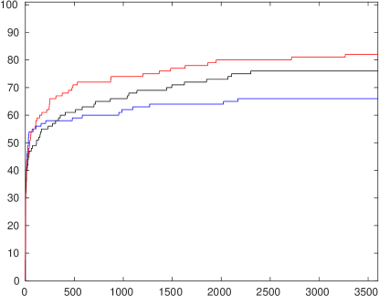
Fig. 3: Results from [356]: running time (in seconds; horizontal axis) versus number of instances solved to optimality (out of 100; vertical axis) for the commercial MIP solver CPLEX [229] applied to the compact spark model (blue), the pure binary-IP spark solver (SparkIP; black) and the combined MIP spark solver (SparkMIP; red); the latter two were implemented in SCIP [192] and employed CPLEX as LP-relaxation solver. CPLEX achieved the smallest final optimality gap 66 times (i.e., only on those instances it could solve to optimality within the time limit, which were also solved by the others), SparkIP 79 times, and SparkMIP 95 times.

A binary IP formulation analogous to (2) can also be given for $\ell_{0}$-min($Ax=b$), based on the following result (we omit its straightforward proof):

Lemma 3.

A set $\emptyset\neq S\subseteq[n]$ is a (inclusion-wise minimal) feasible support for $x$ w.r.t. $Ax=b$ if and only if $S\cap B^{c}\neq\emptyset$ for all (maximal) infeasible supports $B$.

This IP then reads

(3) $$\min\left\{\mathds{1}^{\top}y\,:\,\mathds{1}^{\top}y_{B^{c}}\geq 1\quad\forall\text{(max.) infeas.\ supports }B;\leavevmode\nobreak\ y\in\{0,1\}^{n}\right\}.$$

In fact, Lemma 3 and (3) extend directly to $\ell_{0}$-min($\lVert{Ax-b}\rVert_{\infty}\leq\delta$); however, in contrast to the spark case (2), the separation problem for the inequalities in (3) w.r.t. maximal infeasible supports can be shown to be generally NP-hard [359]. The approach is strongly related to the model from [234] discussed earlier, which essentially splits the support into that of the positive and negative parts of $x$, respectively. This split seems to have some structural advantages w.r.t. greedy separation heuristics, even though the underlying IP has (roughly) twice as many variables due to the transformation to MaxFS/MinIISC.

Note that one can also make use of the spark IP formulation, and (with slight modifications) the solver from [356], to tackle $\ell_{0}$-min($Ax=b$): While $\ell_{0}$-min($Ax=0$, $x\neq 0$) searches for the overall smallest circuit of the vector matroid induced by the columns of $A$, $\ell_{0}$-min($Ax=b$) can be viewed as seeking the smallest circuit of the vector matroid over $(A,-b)$ that mandatorily contains the right-hand-side column (see also [119]). Thus, $\ell_{0}$-min($Ax=b$) is equivalent to

(4) $$\min\quad \mathds{1}^{\top}y$$

s.t. $$\mathds{1}^{\top}y_{B^{c}}\geq 1\quad\forall\,B\subset[n]:\leavevmode\nobreak\ \lvert{B}\rvert=\operatorname{rank}((A_{B},-b))=m,\leavevmode\nobreak\ y\in\{0,1\}^{n},$$

i.e., the covering-type inequalities hold for all complements of bases of the matroid over the columns of $(A,-b)$ that contain $n+1$. Indeed, it can easily be seen that bases containing the $(n+1)$-th column of $(A,-b)$ correspond to infeasible supports (w.r.t. $Ax=b$) from Lemma 3 once that column is removed. While these infeasible supports are not necessarily maximal (there could be columns of $A$ that are linearly dependent on the ones contained in the basis and thus could be included in a linear combination without changing infeasibility), the separation problem can still be solved by a greedy method, unlike for the covering inequalities corresponding to maximal infeasible supports. We will explore big-M selection and the approach to solve $\ell_{0}$-min($Ax=b$) via (4) a bit further as an illustrative example in Section 3.2.1 below.

Besides tightening big-M bounds as discussed earlier, it has been shown in several cardinality minimization applications that standard (general-purpose) branch-and-bound MIP solvers can be improved significantly by exploiting problem-specific heuristics and relaxations (or methods tailored to the specific structure of the relaxations encountered in the process of solving the MIPs), see, e.g., [291, 377, 376, 356]. Of course, this also holds for certain mixed-integer nonlinear programming (MINLP) formulations. An example is the efficient heuristic providing high-quality starting solutions for the exact branch-and-cut scheme (including specialized cuts and branching rules) for $\ell_{0}$-min($\lVert{Ax-b}\rVert_{2}\leq\delta$, $\lvert{x}\rvert\in\{0,1\}$, $x\in\mathds{C}^{n}$) recently proposed in [177].

A general impression, which may be gleaned from all the MIP efforts in the aforementioned references is that finding good or even optimal solutions is often possible with dedicated heuristics (including running MIP solvers for a limited amount of time), but that proving optimality is hard not only in theory but also in practice.

Finally, we point out that cardinality minimization problems could also be solved by means of a sequence of cardinality-constrained problems with $\lVert{x}\rVert_{0}\leq k$ for $k=1,2,\dots$, until the first feasible subproblem is found (indicating minimality of the respective cardinality level); of course, one could also apply, e.g., binary search in this context. Depending on the concrete constraints, since this sequential approach leaves the possibility to choose an arbitrary objective function, one could simplify the feasible set by moving parts of it into the objective—for instance, $\ell_{0}$-min($\lVert{Ax-b}\rVert\leq\delta$) could be tackled by solving $\ell_{0}$-cons($\lVert{Ax-b}\rVert$, $k$, $\mathds{R}^{n}$) for $k=1,2,\dots$ until the first subproblem with optimal objective value of at most $\delta$ was found.

3.2.1 An Illustrative Example

Since (4) appears to be novel, we adapted the spark-specific code from [356] to this variant in order to, in the following, provide an illustrative example on how heavily exploiting problem-specific knowledge can significantly improve the performance of exact solvers versus black-box models. The following example consists of the matrix $A$ from instance 67 from [356] (a $192\times 384$ binary parity-check matrix of a rate-$1/2$ WRAN LDPC code) and a right-hand side $b\coloneqq Ax$, where $x\in\mathds{R}^{384}$ has $30$ nonzero components with positions drawn uniformly at random and entries drawn i.i.d. from the standard normal distribution. The (modified) spark code is implemented using the open-source MIP solver SCIP [192], which we also employ as a black-box solver for the standard big-M formulation of $\ell_{0}$-min($Ax=b$), i.e.,

(5) $$\min\big{\{}\mathds{1}^{\top}y\,:\,Ax=b,\leavevmode\nobreak\ -\mathcal{M}y\leq x\leq\mathcal{M}y,\leavevmode\nobreak\ y\in\{0,1\}^{n}\big{\}}.$$

We will consider different choices of $\mathcal{M}$, to illustrate how the quality of the bounds greatly influences solver efficiency. Specifically, we solve the problem for conservative choices $\mathcal{M}=1000$ and $\mathcal{M}=100$, an “optimistic” choice $\mathcal{M}=10$, as well as $\mathcal{M}=3.9$ (corresponding approximately to the $99.99\%$ quantile of the standard normal distribution) and $\mathcal{M}=2.6$, the largest absolute value of the entries in the generated $x$ (rounded up to one significant digit). Thus, in terms of uniform bounds for all variables, the latter two exploit knowledge of at least the distribution of the ground-truth signal vector $x$ and are unrealistically tight, and highly instance-specific. For the problem-specific IP solver, which does not require big-M values, we illustrate how adding different components that are tailored to the problem under consideration yields an increasingly faster algorithm (we refer to [356] for detailed descriptions and omit stating the straightforward modifications to implicitly handle $Ax=b$ rather than $Ax=0$): Version (i) is characterized by the basic model (4) with separation of covering inequalities as well as generalized-cycle inequalities (but no local cuts), version (ii) adds a propagation routine (to infer, e.g., further variable fixings after branching, and execute problem-specific pruning rules), (iii) additionally incorporates the well-known $\ell_{1}$-minimization problem $\min\{\lVert{x}\rVert_{1}:Ax=b\}$ as a primal heuristic, and finally, in version (iv), we turn off several costly primal heuristics that are part of SCIP but were not helpful (in particular, diving and rounding heuristics). The results are summarized in Table 2; all experiments were run in single-thread mode under Linux on a laptop (Intel Core i7-8565U CPUs 1.8 GHz and 8 GB memory); we used the LP-solver SoPlex 5.0.0 that comes with SCIP 7.0.0 to solve all relaxations.

Table 2: Runtimes and number of node for model/solver variants on the example instance of $\ell_{0}$-min($Ax=b$).

solver/model	$\mathcal{M}$	runtime [s]	nodes
black-box SCIP big-M-MIP	1000	544.1	9503
black-box SCIP big-M-MIP	100	86.6	859
black-box SCIP big-M-MIP	10	43.1	423
black-box SCIP big-M-MIP	3.9	25.5	5
black-box SCIP big-M-MIP	2.6	3.5	1
modified Spark-IP (i)	–	62.2	621
modified Spark-IP (ii)	–	40.7	377
modified Spark-IP (iii)	–	20.7	165
modified Spark-IP (iv)	–	15.6	149

The experiment clearly shows that the black-box approach profits greatly from good big-M values. Nevertheless, it is important to keep in mind that in practical applications, one may not have sufficiently useful information (such as exploiting knowledge of the “signal” distribution to come up with a reasonable guess like $\mathcal{M}=3.9$ in the above example). If, on the other hand, explicit bounds are known for $x$, then the approach may work quite well and is certainly worth a try. However, even if good guesses (like the $3.9$ above) are available, a dedicated problem-specific solver may still achieve significant performance improvements. Here, in its “most sophisticated” variants (iii) and (iv), the modified spark computation code outperforms the black-box solver by at least 20% in terms of running time. Even the more rudimentary version (i) is significantly faster than the big-M approach if no knowledge regarding a good choice of $\mathcal{M}$ is available and one needs to choose a relatively large $\mathcal{M}$ ($100$ or $1000$) to be on the safe side. Finally, note that one could, in principle, merge the two approaches (i.e., use the MIP model (5) with dynamically added cuts derived from (4)); for $\ell_{0}$-min($Ax=0,x\neq 0$), such an approach indeed turned out to be beneficial (see [356]), but recall that there were no big-M selection issues due to scalability of nullspace vectors.

3.3 Cardinality-Constrained Optimization

Naturally, the techniques discussed in Section 3.1 can also be used to reformulate cardinality-constrained problems. For instance, in the presence of variable bounds $\ell\leq x\leq u$ (possibly of a big-M nature), the general problem $\ell_{0}$-cons($f$, $k$, $X$) can be written as

$$\min\left\{f(x)\,:\,Ly\leq x\leq Uy,\leavevmode\nobreak\ \mathds{1}^{\top}y\leq k,\leavevmode\nobreak\ x\in X,\leavevmode\nobreak\ y\in\{0,1\}^{n}\right\},$$

where $U\coloneqq\operatorname{Diag}(u)$ and $L\coloneqq\operatorname{Diag}(\ell)$. Similarly, the reformulations using complementarity-type constraints can be employed in an analogous fashion, although the resulting theoretical properties may differ in some fine points. For the sake of brevity, we omit the straightforward details.

It is also possible to algebraically formulate cardinality constraints on vectors, as well as rank constraints on matrices, using continuous auxiliary variables and a set of linear constraints plus one bilinear inequality, see [222]. Somewhat surprisingly, it seems that these reformulations are not very well known and have, to our knowledge, hardly been employed in practical algorithms thus far. The key result for vector sparsity is [222, Thm. 1]: $x\in\mathds{R}^{n}$ satisfies $\lVert{x}\rVert_{0}\leq k$ if and only if there exist $t\in\mathds{R}$ and $y,q,w\in\mathds{R}^{n}$ such that

$$\lVert{q}\rVert_{1}+(k+1)\lVert{w}\rVert_{\infty}\leq t\leq x^{\top}y,\quad x=q+w,\quad\lVert{y}\rVert_{1}\leq k,\quad\lVert{y}\rVert_{\infty}\leq 1;$$

note that the $\ell_{1}$- and $\ell_{\infty}$-norm terms can be linearized as usual. For the analogous result on rank constraints, see [222, Thms. 2 and 3]. The reformulations from [222] are closely related to the sum of the $k$ largest absolute values of entries in the vector case, or singular values in the matrix case, respectively (see also the “trimmed LASSO” discussed at the end of Section 4.4). A related characterization of a cardinality constraint can be derived from [395], where it is shown that $\lVert{x}\rVert_{0}=\min\{\lVert{u}\rVert_{1}:\lVert{x}\rVert_{1}=x^{\top}u,\leavevmode\nobreak\ -\mathds{1}\leq u\leq\mathds{1}\}$ for any $x\in\mathds{R}^{n}$, so consequently,

(6) $$\lVert{x}\rVert_{0}\leq k\quad\Leftrightarrow\quad\lVert{u}\rVert_{1}\leq k,\leavevmode\nobreak\ \lVert{x}\rVert_{1}=x^{\top}u,\leavevmode\nobreak\ -\mathds{1}\leq u\leq\mathds{1}.$$

It is noteworthy that bound-computation problems may be easier for cardinality-constrained problems than for cardinality-minimization: To ensure validity of computed bounds, it suffices to ensure that a known upper bound on the minimum objective value is not exceeded (cf. [42])—for problems of the class $\ell_{0}$-min($X$), this unfortunately leads to (generally intractable) cardinality constraints. Here, the cardinality constraint can actually be omitted (or, more precisely, relaxed to $\lVert{x}\rVert_{0}\leq n$), so bound-computation problems may look like

$$\inf_{x}/\sup_{x}\left\{x_{i}\,:\,f(x)\leq\bar{f},\leavevmode\nobreak\ x\in X\right\}.$$

For instance, [55] suggests the data-driven bounds $\inf/\sup\{x_{i}:\lVert{Ax-b}\rVert_{2}\leq\bar{f}\}$ for $\ell_{0}$-cons($\lVert{Ax-b}\rVert_{2}$, $k$, $\mathds{R}^{n}$), which are simple convex problems. The required bound $\bar{f}$ on the optimal objective value can be obtained by any heuristic, or possibly analytically.

Thus, in particular, the exact branch-and-cut solvers of [394] (and some earlier works referenced therein) for LPCCs can be used if $f$ is an affine-linear function. Moreover, the polyhedral results (valid inequalities for polytopes with cardinality constraints) from the references given at the end of Section 3.1, as well as the aforementioned branching schemes (e.g., [135]) can also be applied in the present general context. Note that [63] describes a branching rule that allows to avoid auxiliary binary variables.

An exact mixed-binary minimax (or outer-approximation) algorithm was developed in [59, 57] for the sparse SVM problem $\ell_{0}$-cons($L(w,b)$, $k$, $(w,b)\in\mathds{R}^{n+1}$), subsuming a ridge regularization term in $L$ (cf. Section 2.3), with encouraging performance in the context of logistic regression and hinge loss sparse SVM. It was later extended to more general MIQPs, including, in particular, the portfolio selection problem, see [52, 53]. This method is the latest in a series of exact algorithm proposals for variants of MIQPs with cardinality constraints, often focusing on portfolio optimization applications, that includes, in particular, [63, 339, 58, 71, 194, 193, 25, 101, 126]. A recent survey of models and exact methods for portfolio selection tasks, including cases with cardinality constraints, is provided by [289]; another fairly broad overview of MIQP with cardinality constraints can be found in [407]. A MIQP algorithm for the special case of feature selection (or sparse regression), $\ell_{0}$-cons($\lVert{Ax-b}\rVert_{2}$, $k$, $\mathds{R}^{n}$), was proposed in [55], including the aforementioned ways to compute tighter big-M bounds; some statistical properties of such sparse regression problems and relations to their regularized versions are discussed in, e.g., [400, 342]. Other tweaks of the straightforward big-M MIQP approach are discussed in [245] (see also [18]). Introducing a ridge regularization term to the regression objective, [59] recast the problem as a binary convex optimization problem and propose an outer-approximation solution algorithm that scales to large dimensions, at least for sufficiently small $k$. A different (big-M free) MIQP formulations is considered in [383], which also includes an analysis of different relaxation bounds and a numerical comparison with the method from [59] and some existing and novel heuristics in a large-scale setting. A similarly scalable problem-specific branch-and-bound method for a MIQP model of the corresponding regularized problem—i.e., minimizing a weighted objective with an $\ell_{2}$ data fidelity, an $\ell_{0}$ cardinality, and a ridge penalty term—is discussed in [221]. An extension of this method to group sparsity is described in [220], where both exact and approximate solutions are considered. It is also possible to recast cardinality-constrained least-squares problems with ridge penalty as mixed-integer semidefinite programs (MISDPs), see [323, 191], but those can only be solved exactly for small-scale instances, despite providing stronger relaxations. For the sparse PCA problem $\ell_{0}$-cons($x^{\top}Qx$, $k$, $x^{\top}x=1$), two exact MIQP solvers were very recently developed in [144] and [49].

It is also worth mentioning that simple cardinality-constrained problems with separable objective function $\phi(x)=\sum_{i=1}^{n}\phi_{i}(x_{i})$ and $X=X_{1}\times\cdots\times X_{n}$ with $0\in X_{i}$ for all $i$, admit a closed-form solution, see [269].

Portfolio optimization seems to be the showcase example for cardinality constraints. Therefore, in the following, we provide some more details on the formulation of such problems as MIQPs, along with a few numerical experiments to shed some light on their practical solution with black-box MIP solvers.

3.3.1 Illustrative Example: Cardinality-Constrained Portfolio Optimization Problems

The classical Markowitz mean-variance optimization problem (cf. [282]) can be described as follows:

(7) $$\min\big{\{}\lambda x^{\top}Qx-\bar{\mu}^{\top}x\,:\,Ax\geq b\big{\}}.$$

Here, $x\in\mathds{R}^{n}$ is a vector of asset positions, $Q\in\mathds{R}^{n\times n}$ is the sample covariance matrix of asset returns, $\bar{\mu}\in\mathds{R}^{n}$ the vector of average asset returns, $\lambda\geq 0$ is a risk-aversion multiplier, and $Ax\geq b$ are generic linear portfolio construction requirements. The objective of (7) represents a tradeoff between risk and portfolio performance. In the simplest form, the linear requirements for feasible portfolios are

(8a) $$\sum_{j=1}^{n}x_{j}\,=\,1,$$

(8b) $$x\geq 0.$$

In this case, $x_{j}\geq 0$ represents the percentage of a portfolio invested in an asset $j$.

Modern versions of problem (7) incorporate features that require binary variables. There is a large literature that addresses such features, see, e.g. [63, 58, 101]. A critical feature is a cardinality constraint on the number of positions to be taken, e.g., an upper bound on the number of nonzero $|x_{j}|$. Here, we detail typical portfolio optimization/management constraints along with their respective practical motivation and (numerical) aspects to consider when building and solving such models. Moreover, we discuss some experiments using a recent version of the commercial MI(Q)P solver Gurobi [215] on formulations that incorporate several modern features, using real-world data.

• Long-short portfolios. In the modern practice, an asset $j$ can be “long”, “short” or “neutral”, represented, respectively, by $x_{j}>0$, $x_{j}<0$ or $x_{j}=0$. We can write, for any asset $j$, $x_{j}=x^{+}_{j}-x^{-}_{j}$, with the (important) proviso that $x^{+}_{j}x^{-}_{j}=0$. This complementarity constraint provides an example of the use of binary variables, as discussed earlier: The problem will always be endowed with upper bounds on $x^{+}_{j}$ and $x^{-}_{j}$; denote them by $u^{+}_{j}$ and $u^{-}_{j}$, respectively. Then, to ensure $x^{+}_{j}x^{-}_{j}=0$, we write

  (9) $$x^{+}_{j}\leq u^{+}_{j}y_{j},\quad x^{-}_{j}\leq u^{-}_{j}(1-y_{j}),\quad y_{j}\in\{0,1\}.$$

  A portfolio manager may also seek to limit the total exposure in the long and short side. This takes the form of respective constraints

  $$L^{+}\,\leq\,\sum_{j=1}^{n}x^{+}_{j}\,\leq\,U^{+}\quad\text{and}\quad L^{-}\,\leq\,\sum_{j=1}^{n}x^{-}_{j}\,\leq\,U^{-},$$

  for appropriate nonnegative quantities $L^{\pm}$ and $U^{\pm}$. A constraint of the form (8a) does not make sense in a long-short setting; instead one can impose $\sum_{j=1}^{n}(x^{+}_{j}+x^{-}_{j})=1$ (together with (9)). Additionally, one may impose upper and lower bounds on the ratio between the total long and short exposures.

• Portfolio update rules. In a typical portfolio management setting, a portfolio is being updated rather than constructed “from scratch”. Each asset $j$ has an initial position $x^{0}_{j}$ which could itself be long, short or neutral. Thus, we can write

  $$x_{j}\ =\ x^{0}_{j}+\delta^{+}_{j}-\delta^{-}_{j},$$

  where $\delta^{+}_{j}\geq 0$ and $\delta^{-}_{j}\geq 0$ are the changes in the long and short direction, respectively. These quantities may themselves be (individually) upper- and lower-bounded, and the same may apply to the sums $\sum_{j=1}^{n}\delta^{+}_{j}$ and $\sum_{j=1}^{n}\delta^{-}_{j}$.

• Cardinality constraints. As stated above, a typical requirement is to place an upper bound on the number of nonzero positions $x_{j}$. We can effect this through the use of binary variables, by repurposing the binary variable $y_{j}$ introduced above, introducing a new binary variable $z_{j}$, and imposing

  $$x^{+}_{j}\leq u^{+}_{j}y_{j},\quad x^{-}_{j}\leq u^{-}_{j}z_{j},\quad z_{j}\leq 1-y_{j},\quad z_{j}\in\{0,1\},$$

  $$\sum_{j=1}^{n}(y_{j}+z_{j})\ \leq\ k,$$

  where $k>0$ is the upper bound on the number of nonzero positions. However, this is not the only case a cardinality constraint may be needed. Such rules may also apply, for example, to specific subsets of assets (e.g., within a certain industrial sector).

• Threshold rules. When $n$ is large and $\lambda$ is large, the standard mean-variance problem may produce portfolios that include assets in minute quantities. Hence, a manager may seek to enforce a rule that states that an asset is either neutral (i.e. $x_{j}=0$) or takes a position that is “large enough”, resulting in so-called semi-continuous variables. We can reuse the binary variables just described, for this purpose: For any asset $j$, we constrain

  $$x^{+}_{j}\geq\theta^{+}_{j}y_{j}\quad\mbox{and}\quad x^{-}_{j}\geq\theta^{-}_{j}z_{j},$$

  where $\theta^{+}_{j}$ and $\theta^{-}_{j}$ are the respective threshold values. In addition, we may apply similar rules to the $\delta^{\pm}$ quantities introduced above (so as to deter unnecessary movements).

• Reduced-rank approximations of the sample covariance matrix $Q$. Typical covariance matrices arising in portfolio management have high rank (usually, full rank) but with many tiny eigenvalues. In fact, the spectrum of such matrices displays the usual “real-world” behavior of rapidly declining eigenvalues. For instance, if $n=1000$ (say), only the top $200$ eigenvalues may be significant, and of those, the top $50$ will dominate. Usually the top eigenvalue is significantly larger than the second largest, and so on.

  Let us consider the spectral decomposition of $Q=V\Omega V^{\top}$, where $V$ is the $n\times n$ matrix whose columns are the eigenvectors of $Q$ and $\Omega=\operatorname{diag}(\omega_{1},\omega_{2},\ldots,\omega_{n})$ is the diagonal matrix holding the respective eigenvalues $\omega_{1}\geq\omega_{2}\geq\ldots\geq\omega_{n}\ (\geq 0)$. We can then approximate

  (10) $$Q\approx\sum_{i=1}^{H}\omega_{i}v_{i}v_{i}^{\top},$$

  where $v_{i}$ is the $i$-th eigenvector of $Q$ and $H\leq n$ is appropriately chosen. The primary reason (as seen by practitioners) for replacing the sample covariance matrix with the approximation in (10) is that by doing so one removes “noise”, i.e., that one obtains a better representation of the “true” underlying covariance matrix.

  Denoting by $V^{H}$ the $H\times n$ matrix whose $i$-th row (for $1\leq i\leq H$) is $v_{i}^{\top}$, the objective of problem (7) can be written as

  (11) $$\min\quad \lambda\sum_{i=1}^{H}\omega_{i}f^{2}_{i}-\bar{\mu}^{\top}x,$$

  where the $f_{i}$ are new variables, subject to the constraint $V^{H}x=f$. As stated above, the choice of $H$ hinges on how quickly the eigenvalues $\omega_{i}$ decrease. A prematurely small choice for $H$ may result in a poor approximation to $Q$, and a large choice yields a formulation with very small parameters. One can overcome these issues by relying on the residuals, that is to say the quantities

  (12) $$\rho_{j}\ \coloneqq\left(Q-\sum_{i=1}^{H}\omega_{i}v_{i}v_{i}^{\top}\right)_{jj}=\ Q_{jj}-\sum_{i=1}^{H}\omega_{i}v_{ij}^{2},\quad j\in[n].$$

  These quantities are nonnegative since $Q-\sum_{i=1}^{H}\omega_{i}v_{i}v_{i}^{\top}=\sum_{i=H+1}^{n}\omega_{i}v_{i}v_{i}^{\top}$ is positive semidefinite. Moreover, in general, the $\rho_{j}$ should be small if the approximation (10) is good (namely, since $\sum_{i=H+1}^{n}\omega_{i}v_{i}v_{i}^{\top}$ is diagonal-dominant). The residuals can be used to update the objective (11) as follows:

  (13) $$\min\quad \lambda\sum_{i=1}^{H}\omega_{i}f^{2}_{i}\,+\lambda\sum_{j=1}^{n}\rho_{j}x_{j}^{2}\ \ -\ \bar{\mu}^{\top}x.$$

  Some of the $\rho_{j}$ may be extremely small—in such a case, it is numerically convenient to replace them with zeros.

3.3.2 Portfolio Optimization Example: Experiments

We next outline the results on a challenging instance with the following attributes:

• $n=741$ with data from the Russell 1000 Index (made publicly available by the authors of [52])

• Full covariance matrix

• Cardinality limit $k=50$ with all threshold values set at $\theta^{+}_{j}=\theta^{-}_{j}=0.01$

• Long-short model with maximum and minimum long exposures set at $U^{+}=0.5$ and $L^{+}=0.4$, respectively, and maximum short exposure set at $U^{-}=0.2$ (and no minimum short exposure, i.e., $L^{-}=0$)

The above formulation was run using Gurobi 9.1.1 on a machine with 20 physical cores (Intel Xeon E5-2687W v3, 3.10 GHz) and 256 GB of RAM. Table 3 summarizes the observed performance using default settings.

Table 3: Behavior of solver on cardinality-constrained portfolio optimization problem.

nodes	incumbent	best bound	gap	runtime [s]
0	25.40531	0.53332	97.9$\%$	14
0	0.86096	0.53332	38.1$\%$	18
15	0.78644	0.54223	31.1$\%$	25
5611	0.72123	0.55025	23.7$\%$	92
11838	0.71995	0.55025	23.6$\%$	130
106774	0.71904	0.57292	20.3$\%$	500
242365	0.71898	0.57873	19.5$\%$	1000
524934	0.71898	0.58455	18.7$\%$	2002
817290	0.71898	0.58788	18.2$\%$	3002
994932	0.71898	0.58946	18.0$\%$	3605

Let us consider now the outcome when we run the same portfolio optimization problem, but now using the approximation to the covariance matrix obtained by taking the top $H=250$ modes. In this case, the top eigenvalue equals $8.10\times 10^{-2}$ while the $250^{\text{th}}$ is approximately $1.57\times 10^{-4}$. Table 4 summarizes the results.

Each table provides relevant statistics concerning the corresponding run; the rows were selected to highlight significant steps within the run (e.g., discovery of a new incumbent or improvement of the best lower bound) so as to provide the reader with a qualitative understanding of the progress made by the solver.

Table 4: Behavior of solver on approximation to instances in Table 3 obtained by using $H=250$ modes.

nodes	incumbent	best bound	gap	runtime [s]
0	4.98030	-0.00080	100.0$\%$	6
217	2.08509	0.00009	100.0$\%$	39
562	0.69882	0.00009	100.0$\%$	52
924	0.31362	0.00009	100.0$\%$	80
1048	0.31362	0.31293	0.2$\%$	105
1067	0.31362	0.31362	0.0$\%$	116

In the first case, we ended the solving run after approximately one hour of elapsed time with a remaining optimality gap of about 18 %. In the second case (cf. Table 4), the solver is able to close the gap so as to attain optimality within tolerance after about two minutes. We stress that such reduced-rank problems are not always significantly easier than their full-rank counterparts, but, overall, they prove more practicable on average. The objective value of a solution as per the rank-reduced problem is a lower bound for its value in the true problem (since we are ignoring positive terms in the spectral expansion of the covariance matrix), but beyond this simple statement, an accurate estimation of how close this lower bound actually is can be nontrivial.

More importantly, a portfolio manager would prefer a rank-reduced formulation because the modes being ignored are quite small and hence may seem negligible. However, it is important to note that this reasoning does not amount to a mathematically correct statement. Indeed, note that the best lower bound after one hour in Table 3 is notably larger than the optimal value of the approximated problem in Table 4.

An additional and important aspect of this discussion that we are not addressing is the practical impact on portfolio management that a reduced-rank representation will have. A portfolio manager will not simply be interested in solution speed—rather, the performance of the resulting portfolio is of great interest. This point is significant in the sense that the covariance matrix $Q$, and, of course, the spectral decomposition $Q=V\Omega V^{\top}$, are data-driven. Both objects are bound to be very “noisy”, for lack of a better term. It can be observed that (in particular) the leading modes of $Q$ (i.e., the columns of the matrix $V^{H}$) can be quite noisy. A closely related issue concerns the number of modes $H$ to rely on. The proper way to handle such noise is by applying some form of robust optimization, see [202], but an in-depth analysis of these topics is outside the scope of the present work.

3.4 Cardinality Regularization Problems

There appears to be hardly any literature focusing specifically on the exact solution of regularized cardinality minimization problems, $\ell_{0}$-reg($\rho$, $X$). As mentioned earlier, [170] contains theoretical optimality conditions (but no exact algorithm) for $\ell_{0}$-reg($\tfrac{1}{\gamma}f(x)$, $g(x)=0,h(x)\leq 0$) with $\gamma>0$ and continuously differentiable functions $f:\mathds{R}^{n}\to\mathds{R}$, $g:\mathds{R}^{n}\to\mathds{R}^{p}$, and $h:\mathds{R}^{n}\to\mathds{R}^{q}$. Similarly, [269] considers such problems allowing for additional constraints that form a closed convex set $X$. They also show that for separable $f$ and constraints representable as $X_{1}\times\cdots\times X_{n}$ with $0\in X_{i}$ for all $i$, the $\ell_{0}$-regularized problem admits a closed-form solution. A statistical discussion of (solution properties of) least-squares regression with cardinality regularization, $\ell_{0}$-reg($\tfrac{1}{2\lambda}\lVert{Ax-b}\rVert_{2}^{2}$, $\mathds{R}^{n}$), as well as other concave regularizers, can be found in [400] (albeit without algorithmic results) and suggests that from a statistical perspective, cardinality-constrained least-squares regression is preferable to its cardinality-regularized variants.

In the cosparsity model, the problem of one-dimensional “jump-penalized” least-squares segmentation,

$$\min\tfrac{1}{2}\lVert{b-x}\rVert_{2}^{2}+\lambda\lVert{Bx}\rVert_{0},$$

where $B$ is the difference operation (so that $\lVert{Bx}\rVert_{0}=\sum_{i=2}^{n}\chi_{\{x_{i}\neq x_{i-1}\}}$) and $\lambda>0$, can be solved in polynomial time, see [233, 77] and references therein. Similarly, if $B$ encodes more general adjacency relations between entries of $x$,

$$\min\big{\{}\tfrac{1}{2}\lVert{b-x}\rVert_{2}^{2}+\lambda\lVert{Bx}\rVert_{2}^{2}+\mu\lVert{x}\rVert_{0}\,:\,x\geq 0\big{\}}$$

(with $\lambda$, $\mu>0$) admits a polynomial-time solution, while for the variant with a cardinality constraint $\lVert{x}\rVert_{0}\leq k$ instead of the second regularization term, no such methods are known and MIQP techniques can be applied, see [19] and the previous works detailed therein.

Generally, the techniques from Section 3.2 are applicable to regularized cardinality problems as well: If, for instance, auxiliary binary variables $y\in\{0,1\}^{n}$ are used to reformulate $\lVert{x}\rVert_{0}$ as $\mathds{1}^{\top}y$ (coupling $x$ and $y$ via, e.g., big-M constraints), one can simply integrate the regularization term into the new objective $\mathds{1}^{\top}y+\rho(x)$. Depending on the concrete choice of the function $\rho$, mixed-integer linear or nonlinear programming can then be applied analogously.

Similarly, some techniques from Section 3.3 might also be applicable in the regularization context after reformulating $\ell_{0}$-reg($\rho$, $X$) as

$$\min_{t,x}\left\{t\,:\,\lVert{x}\rVert_{0}+\rho(x)\leq t,\leavevmode\nobreak\ x\in X,\leavevmode\nobreak\ t\geq 0\right\}.$$

However, $\lVert{x}\rVert_{0}\leq t-\rho(x)$ is obviously not a classical cardinality constraint, as the right-hand side also depends on $x$ and $t\geq 0$ is a variable. We are not aware of any work investigating this type of mixed constraint.

Finally, [148] considers $\ell_{0}$-reg($\rho$, $X$) and derives an exponential-size convexification through disjunctive programming. Based on this convexification, the authors propose a class of penalty functions called “perspective penalties” that are the counterpart of the perspective relaxation well-known in the mixed-integer nonlinear context [214]. Computational experiments comparing various lower bounds (including those from [323]) are discussed. A similar convexification attempt is considered in [378], but this time applied to the setting in which the cardinality is explicitly modeled via $x_{i}(1-y_{i})=0\leavevmode\nobreak\ \forall i\in[n]$ with $y$ binary. The convexification is then obtained by exploiting the interplay between non-separable convex objectives and combinatorial constraints on the indicator variables; some computational results on real-world datasets are reported as well.

4 Relaxations and Heuristics

Most of the exact solution methods mentioned in the last section make use of problem-specific heuristics and/or efficient ways to solve the encountered relaxations. Indeed, incorporating such components into dedicated MIP and MINLP algorithms (along with other aspects like propagation and branching rules or cutting planes) can drastically improve performance compared to black-box approaches with general-purpose solvers, see, e.g., [57, 49, 356], or the example for $\ell_{0}$-min($Ax=b$) in Section 3.2.1.

Additionally, heuristic methods are of interest in their own rights, as they are often (at least empirically) able to provide good-quality solutions in fractions of the sometimes considerable runtime an exact mixed-integer programming approach may take, and therefore also open the possibility—or sometimes the only reasonable way—to tackle very high-dimensional, large-scale instances (see also Section 5).

Thus, in this section, we attempt to survey the countless heuristics, relaxation and approximation methods proposed for the various cardinality problems discussed in Section 2. We begin with the well-known $\ell_{1}$-norm surrogate for the cardinality in Section 4.1, devoting subsections to the reasons for its success and the many different (classes of) algorithms that have been proposed for various $\ell_{1}$-problems. Due to the sheer number of results, variations, and improvements, in Section 4.1.1 we limit ourselves to some key results that exhibit the general flavor of so-called “recovery guarantees” and introduce some of the most important concepts. Then, in Section 4.1.2, we give an extensive (though likely still not exhaustive) overview of algorithmic approaches to solve $\ell_{1}$-minimization problems; earlier, but less comprehensive, overviews can also be found in, e.g., [184, 22, 268]. Moving beyond $\ell_{1}$, we subsequently discuss the more general concept of atomic norms (Section 4.2) and further approximations of cardinality objectives (Section 4.3) and constraints (Section 4.4). Finally, Section 4.5 survey greedy-like and miscellaneous other heuristics. We remark that readers who are already very familiar with $\ell_{1}$-norm theory and algorithms might want to skip Section 4.1 and may find the results/tools of the later sections, some of which are fairly new and/or perhaps less known, more useful.

Note that the polyhedral results mentioned in the previous section, i.e., valid inequalities for various kinds of cardinality problems, can be viewed as a means to strengthen the respective LP (or other) relaxations, and could quite possibly be combined with many heuristic- and/or relaxation-based approaches. For brevity, we do not repeat the pointers to the literature in this context. Such integration possibilities appear to have been largely overlooked thus far, and might offer an interesting avenue for future refinements of existing inexact models and algorithms.

4.1 $\ell_{1}$-Norm Surrogates: Basis Pursuit, LASSO, etc.

The most popular relaxation technique replaces the so-called $\ell_{0}$-norm by the “closest” convex real norm—the $\ell_{1}$-norm. Indeed, it is easily seen that

$$\lim_{p\searrow 0}\lVert{x}\rVert_{p}^{p}=\lim_{p\searrow 0}\sum_{i=1}^{n}\lvert{x}\rvert^{p}=\lVert{x}\rVert_{0}.$$

This sentiment along with empirical observations led to the wide-spread use of the $\ell_{1}$-norm as a tractable surrogate to promote sparsity, and has since been underpinned with various theoretical results on when such approaches work correctly, see, e.g., [184] for an overview of breakthrough results in the field of compressed sensing.

In sparse regression, compressed sensing, and statistical estimation, the following incarnations of such $\ell_{1}$-based problems are encountered most often:

(BP($$X \min\quad \lVert{x}\rVert_{1}\quad\text{s.t.}\quad Ax=b,\leavevmode\nobreak\ x\in X;$$))

(BPDN($$\delta,X \min\quad \lVert{x}\rVert_{1}\quad\text{s.t.}\quad\lVert{Ax-b}\rVert_{2}\leq\delta,\leavevmode\nobreak\ x\in X;$$))

(LASSO($$\tau,X \min\quad \tfrac{1}{2}\lVert{Ax-b}\rVert_{2}^{2}\quad\text{s.t.}\quad\lVert{x}\rVert_{1}\leq\tau,\leavevmode\nobreak\ x\in X;$$))

($$\ell_{1} \lambda,X \min\quad \lVert{x}\rVert_{1}+\tfrac{1}{2\lambda}\lVert{Ax-b}\rVert_{2}^{2}\quad\text{s.t.}\quad x\in X.$$-LS())

The basis pursuit problem BP($X$) was first discussed and proven to provide sparse solutions for underdetermined linear equations in [110]. Usually, $X=\mathds{R}^{n}$ here, but the nonnegative ($X=\mathds{R}^{n}_{+}$), bounded ($\ell\leq x\leq u$), complex ($X=\mathds{C}^{n}$), or integral ($X\subseteq\mathds{Z}^{n}$) settings have also been investigated, see, e.g., [156, 184, 258, 244]. The basis pursuit denoising problem BPDN($\delta,X$) extends the noise-free model BP($X$) by allowing deviations from exact equality and thus providing robustness against measurement noise as well as the possibility to achieve even sparser solutions. As for the original cardinality minimization problem, other norms than the $\ell_{2}$-norm have been considered for the constraints, e.g., the $\ell_{\infty}$-norm in [82] or the $\ell_{1}$-norm in [237]. The least absolute shrinkage and selection operator LASSO($\tau,X$) was motivated in a regression context as a way to improve prediction accuracy and interpretability by promoting shrinkage (and thus, ultimately, sparsity) of the predictor variables [353]; it can be seen as the $\ell_{1}$-approximation to the cardinality-constrained least-squares problem. Finally, the $\ell_{1}$-regularized least-squares problem $\ell_{1}$-LS($\lambda,X$) is often employed as well, especially if no immediate bounds $\delta$ or $\tau$ for the related BPDN or LASSO problems are known, and because it is an unconstrained problem (provided $X=\mathds{R}^{n}$) and thus potentially can be solved even more efficiently. In fact, in contrast to the associated $\ell_{0}$-based problems (cf. Prop. 1), it is known that BPDN($\delta,\mathds{R}^{n}$), LASSO($\tau,\mathds{R}^{n}$) and $\ell_{1}$-LS($\lambda,\mathds{R}^{n}$) are always equivalent for certain values of the parameters $\delta$, $\tau$ and $\lambda$ (see, e.g., [363]), although the precise values for which this holds are data-dependent and generally unknown a priori. The recent work [48] analyzes the stability of these programs w.r.t. parameter choices in a denoising setting with $A=I$, and indicates that the regularized version behaves most robustly. In all these problems, typically $X=\mathds{R}^{n}$, though like for BP($X$), other constraints are occasionally considered as well.

Two more $\ell_{1}$-minimization problem variants that have turned out to be of special interest in some applications are the so-called Dantzig Selector [98]

(DS($$\varepsilon,X \min\quad\lVert{x}\rVert_{1}\quad\text{s.t.}\quad\lVert{A^{\top}(Ax-b)}\rVert_{\infty}\leq\varepsilon,\leavevmode\nobreak\ x\in X,$$))

whose cardinality-minimization counterpart was proposed in [284], and the Tikhonov/ ridge-regularized $\ell_{1}$-LS problem

(EN($$\lambda_{1},\lambda_{2},X \min\quad\lVert{x}\rVert_{1}+\tfrac{1}{2\lambda_{1}}\lVert{Ax-b}\rVert_{2}^{2}+\tfrac{\lambda_{2}}{\lambda_{1}}\lVert{x}\rVert_{2}^{2}\quad\text{s.t.}\quad x\in X,$$))

known as the elastic net [409]. The additional ridge penalty here ensures strong convexity of the objective function and, consequently, uniqueness of the minimizer. Like $\ell_{1}$-LS($\lambda,X$), EN($\lambda_{1},\lambda_{2},X$) has been used in several applications such as portfolio optimization [57] or support vector machine learning [373].

In the following, we first provide a very brief overview of the theoretical success guarantees that led to the popularity of $\ell_{1}$-formulations, and then discuss algorithms.

4.1.1 Dipping a Toe Into Why $\ell_{1}$-Reformulations Became Popular

Nowadays, using the $\ell_{1}$-norm as a tractable surrogate for the cardinality is commonplace. This rise to popularity was in large part fueled by the advent of compressed sensing, the signal processing paradigm that reduces measurement acquisition efforts at the cost of more complex signal reconstruction. Low cardinality of signal vectors (i.e., sparsity) has proven to be key for solving the nontrivial recovery problems, and [110] laid essential groundwork in demonstrating that the $\ell_{1}$-surrogate offers a viable and efficient alternative to the “true sparsity” represented by the $\ell_{0}$-norm and associated NP-hard reconstruction tasks. Most of the earliest sparse recovery research focused on the problems BP($\mathds{R}^{n}$) and BPDN($\delta,\mathds{R}^{n}$), so for the sake of exposition, we highlight them and their $\ell_{0}$ counterparts $\ell_{0}$-min($Ax=b$) and $\ell_{0}$-min($\lVert{Ax-b}\rVert_{2}\leq\delta$) here, too. The interesting setup in compressed sensing has $A\in\mathds{R}^{m\times n}$ with $\operatorname{rank}(A)=m<n$, so the system $Ax=b$ is underdetermined and has infinitely many solutions. Sparsity is key to overcome this ill-posedness by allowing, in principle, the exact reconstruction of sufficiently sparse signals as the respective unique sparsest solutions to $Ax=b$, i.e., unique optimal solutions of $\ell_{0}$-min($Ax=b$). As mentioned earlier (cf. Section 2.1), this uniqueness requires that the signal cardinality is smaller than $\operatorname{spark}(A)/2$, regardless of any algorithm being used to solve the actual reconstruction problem, see, e.g., [151].

Although proven to be NP-hard only much later in [360], computing the spark was deemed intractable early on, and since cardinality minimization problems like $\ell_{0}$-min($\lVert{Ax-b}\rVert_{2}\leq\delta$) were already known to be NP-hard as well (cf. [195, 302]), the focus quickly shifted to alternative conditions that ensure sparse solution uniqueness and/or reconstruction error analysis of surrogate methods, in particular $\ell_{1}$-minimization.

The best-known such recovery conditions can all be formulated using a few key matrix parameters, namely:

• The mutual coherence of a matrix $A$,

  $$\mu(A)\coloneqq\max_{\begin{subarray}{c}i,j\in[n],\\ i\neq j\end{subarray}}\frac{\lvert{A_{i}^{\top}A_{j}}\rvert}{\lVert{A_{i}}\rVert_{2}\,\lVert{A_{j}}\rVert_{2}}.$$

• The order-$k$ nullspace constant ($k$-NSC) of a matrix $A$,

  $$\alpha_{k}\coloneqq\max_{x,S}\left\{\,\lVert{x_{S}}\rVert_{1}\,:\,Ax=0,\leavevmode\nobreak\ \lVert{x}\rVert_{1}=1,\leavevmode\nobreak\ S\subseteq[n],\leavevmode\nobreak\ \lvert{S}\rvert\leq k\,\right\}.$$

• The order-$k$ restricted isometry constant ($k$-RIC) of a matrix $A$,

  $$\delta_{k}\coloneqq\min_{x}\left\{\,\delta\,:\,(1-\delta)\lVert{x}\rVert_{2}^{2}\leq\lVert{Ax}\rVert_{2}^{2}\leq(1+\delta)\lVert{x}\rVert_{2}^{2}\leavevmode\nobreak\ \forall x\text{ with }1\leq\lVert{x}\rVert_{0}\leq k\,\right\}.$$

For a $k$-sparse solution $\hat{x}$ of $Ax=b$, these parameters can all be used to certify uniqueness of $\hat{x}$ as the sparsest solution, for instance via $2k<1+1/\mu(A)^{2}$ [263], $\alpha_{k}<1/2$ [152], or $\delta_{2k}<1$ [97, 94]—indeed, these conditions each imply $k<\operatorname{spark}(A)/2$. Yet more interestingly, these parameters also yield recovery conditions for $\ell_{1}$-minimization and other (algorithmic) approaches, i.e., they can be used to ensure correctness of the solutions to surrogate problems (possibly up to certain error bounds) w.r.t. the original sparsity target. In particular, uniform sparse recovery conditions (SRCs) such as incoherence (small enough $\mu(A)$), the nullspace property (NSP) or the restricted isometry property (RIP) ensure $\ell_{0}$-$\ell_{1}$-equivalence for all $k$-sparse vectors, i.e., that the solution to BP($\mathds{R}^{n}$) is unique and coincides with the unique solution of $\ell_{0}$-min($Ax=b$). Besides uniform SRCs, there are also various individual SRCs that establish uniqueness of, e.g., BP($\mathds{R}^{n}$)-solutions for specific $\hat{x}$. The most powerful one in this regard is sometimes called strong source condition [209]: $\hat{x}$ is the unique optimal solution to BP($\mathds{R}^{n}$) if and only if $\operatorname{rank}(A_{\operatorname{supp}(\hat{x})})=\lVert{\hat{x}}\rVert_{0}$ and there exists a vector $w$ with $A^{\top}w\in\partial\lVert{\hat{x}}\rVert_{1}$ such that $\lvert{(A^{\top}w)_{j}}\rvert<1$ for all $j\notin\operatorname{supp}(\hat{x})$. (This condition can be derived via first-order optimality and complementary slackness.) Similarly to uniform SRCs, the strong source condition has its analogues for other $\ell_{1}$-problems like BPDN($\delta,\mathds{R}^{n}$), $\ell_{1}$-LS($\lambda,\mathds{R}^{n}$), LASSO($\tau,\mathds{R}^{n}$), and their “analysis/cosparse counterparts” (with $\lVert{Bx}\rVert_{1}$ instead of $\lVert{x}\rVert_{1}$ for some matrix $B$), see, e.g., [402].

Fig. 4: Illustration of relations between matrix properties and associated SRCs, and their implications w.r.t. recovery of $k$-sparse solutions of $\ell_{0}$-min($Ax=b$) and BP($\mathds{R}^{n}$). (Adapted from [354].)

The strongest SRCs are known for basis pursuit, i.e., BP($\mathds{R}^{n}$); we illustrate some such conditions and their relationships in Figure 4. This figure was adapted from [354], where many more details about recovery conditions are described, with a focus on BP($\mathds{R}^{n}$) and computational complexity.

Regarding other $\ell_{1}$-problems, in particular BPDN($\delta,\mathds{R}^{n}$) or $\ell_{1}$-LS($\lambda,\mathds{R}^{n}$), we refer to [184] and the concise summary, derivations, and references therein; the following is an example of the noise-aware recovery conditions one can find in this context. Let $\sigma_{k}(x)_{p}=\inf\{\lVert{x-z}\rVert_{p}:\lVert{z}\rVert_{0}\leq k\}$ be the $\ell_{p}$-norm error of the best $k$-term approximation of a vector $x\in\mathds{C}^{n}$; this comes into play in situations where $x$ is not exactly sparse (see also [121]). Let a matrix $A\in\mathds{C}^{m\times n}$ satisfy

$$\lVert{y_{S}}\rVert_{2}\leq\frac{\rho}{k^{1/2}}\lVert{y_{S^{c}}}\rVert_{1}+\tau\lVert{Ay}\rVert_{2}\qquad\forall y\in\mathds{C}^{n}\leavevmode\nobreak\ \forall S\subseteq[n]:\lvert{S}\rvert\leq k,$$

where $\rho\in(0,1)$ and $\tau>0$ are constants; this is called the $\ell_{2}$-robust nullspace property of order $k$. Then (see [184, Thm. 4.22]), for any $\hat{x}\in\mathds{C}^{n}$, a solution $x^{*}$ of BPDN($\delta$,$\mathds{C}^{n}$) with $b=A\hat{x}+e$ and $\lVert{e}\rVert_{2}\leq\delta$ recovers the vector $\hat{x}$ with an $\ell_{p}$-error ($1\leq p\leq 2$) of at most

$$\lVert{x^{*}-\hat{x}}\rVert_{p}\leq\frac{\alpha}{k^{1-1/p}}\sigma_{k}(\hat{x})_{1}+\beta k^{1/2-1/p}\delta,$$

for some constants $\alpha,\beta>0$ that depend solely on $\rho$ and $\tau$.

Another typical kind of question investigated in compressed sensing pertains to the number of measurements, i.e., the number of rows of $A$, that are needed to ensure recovery of $k$-sparse vectors by $\ell_{1}$-approaches (and others). The arguments typically use the same matrix parameters as before, with an apparent focus on restricted isometry properties of random matrices. Briefly, it can be shown for Gaussian (and other) random matrices that $\ell_{0}$-$\ell_{1}$-equivalence for $k$-sparse vectors holds with high probability if $m\geq C(\delta_{k})k\log(n/k)$, where $C(\delta_{k})$ is a constant depending only on the order-$k$ RIC; see [184, Chapter 9]. Very many similar results establish that for sufficiently many random measurements of some kind, one of the (deterministic) sparse recovery conditions holds with high probability. A slightly different approach is taken in [131], where it is shown how to relax the standard NSP into one that holds with high probability under certain distributional assumptions on the nullspace (rather than the sensing matrix itself), and relate the task of verifying this condition to classical combinatorial optimization problems.

These types of results laid the foundation for the success of $\ell_{1}$-approximations to sparsity, or cardinality terms, and gave rise to a huge amount of research, both on theoretical improvements and efficient algorithms for various problem variants. In order to not dilute the focus of the present paper too much, we do not delve further into the theory outlined above, and refer to [184, 256, 164, 150] as good starting points for anyone wishing to dig deeper. We will, nonetheless, complement the present primer with an overview of the various algorithms for $\ell_{1}$-norm optimization problems in the following subsection.

4.1.2 Algorithmic Approaches to $\ell_{1}$-Problems

A plethora of different solution methods have been applied and specialized to efficiently handle one or more of the above problems or slight variations. It is noteworthy that most methods are first-order methods that often do not need the matrix $A$ to be given explicitly and can instead work with fast operators implementing matrix-vector products with $A$ and/or $A^{\top}$. This enables application of such algorithms in large-scale regimes and special settings where $A$ corresponds to, e.g., a fast Fourier transform. Moreover, the algorithms can often handle complex data and variables as well; for simplicity, we again focus only on the real-valued setting.

For clarity, we group the different approaches according to the broader categories they fall into:

Reformulation as LPs or SOCPs

It is well known that the absolute value function, and thus, by extension, the $\ell_{1}$-norm, can be linearized. Hence, any problem involving only linear and $\ell_{1}$-norm terms in the objective and the constraints can be written as a linear program (LP). Similarly, convex $\ell_{2}$-norm terms (as in, e.g., BDPN($\delta,\mathds{R}^{n}$)) can be reformulated using second-order cone techniques, yielding second-order cone programs (SOCPs). For both these classes, there are well-known standard solution methods like simplex method variants (for LPs), active-set or interior point algorithms (for both), see, e.g., [365, 76], with highly sophisticated genera-purpose implementations (e.g., [229, 215, 382, 192]).

Namely, $\ell_{1}$-magic (see [92]) employs the generic primal-dual interior point solver from [76] to solve the LP reformulation

$$\min\leavevmode\nobreak\ \mathds{1}^{\top}u\quad\text{s.t.}\quad Ax=b,\leavevmode\nobreak\ -u\leq x\leq u$$

of BP($\mathds{R}^{n}$). This approach has also been applied to some related problems that can be written as LPs, such as DS($\varepsilon,\mathds{R}^{n}$), and, analogously (using another general-purpose log-barrier algorithm from [76]), to problems such as BPDN($\delta,\mathds{R}^{n}$) or total-variation minimization that can be recast as SOCPs. Similarly, SolveBP, described in [110, 111], solves (a perturbed version of) the alternative LP reformulation of BP($\mathds{R}^{n}$) with variable splits, i.e.,

(14) $$\min\leavevmode\nobreak\ \mathds{1}^{\top}x^{+}+\mathds{1}^{\top}x^{-}\quad\text{s.t.}\quad Ax^{+}-Ax^{-}=b,\leavevmode\nobreak\ x^{\pm}\geq 0,$$

by employing the primal-dual log-barrier solver PDCO (based on [200]), which can also handle other problems via suitable LP- or SOCP-reformulations, e.g., BPDN($\delta,\mathds{R}^{n}$).

For $\ell_{1}$-minimization problems with linear constraints $Ax=b$ or $\lVert{Ax-b}\rVert_{p}\leq\delta$ with $p\in\{1,\infty\}$ (as well as some related problems such as the “least absolute deviation (LAD)-Lasso” $\min\{\lVert{Ax-b}\rVert_{1}\,:\,\lVert{x}\rVert_{1}\leq\tau\}$, cf. [370]), it has been proposed in [318] to employ the parametric simplex method [128, 365]. (The earlier version [317] of [318] contains more details and applications.) Note that any implementation will face the typical challenges of a simplex solver—efficient basis updates, cycling avoidance, etc.—and is therefore nontrivial. For similarities with and differences to the related homotopy methods discussed below, see the discussion in [82].

The recent contribution [285] demonstrates that $\ell_{1}$-problems, recast as LPs—in particular, BP($\mathds{R}^{n}$) and DS($\tau,\mathds{R}^{n}$)—can be solved very efficiently by using column generation (cf. [143]) and dynamic constraint generation (i.e., cutting planes). The suggested method initializes the variable and constraint index sets to be included in the first master problem based on the (efficiently obtainable) solution of the homotopy method for $\ell_{1}$-LS($\lambda,\mathds{R}^{n}$). Afterwards, violated but not yet included constraints are identified and added to the model and new variables are added by solving a classical LP-based pricing problem. Iterating over the resulting sequence of smaller subproblems is demonstrated to yield the optimum for the original problem at hand much faster than directly solving it as an LP or with an alternating direction scheme (see below). The same idea, i.e., column (and constraint) generation based on LP reformulations, was also proposed recently for $\ell_{1}$-regularized training of SVMs, see [139].

Finally, l1_ls, described in [249], is an interior-point (primal log-barrier) solver for problems of the form $\ell_{1}$-LS($\lambda,\mathds{R}^{n}$) or $\ell_{1}$-LS($\lambda,\mathds{R}^{n}_{+}$); the algorithm employs a truncated Newton subroutine to obtain approximate search directions.

Homotopy Methods

Homotopy methods for $\ell_{1}$-minimization problems have been described in, e.g., [312, 277, 17, 157]. The basic idea is to directly and efficiently identify breakpoints of the piecewise-linear solution path of $\ell_{1}$-LS($\lambda,\mathds{R}^{n}$), following changes in $\lambda$ from $\lambda\geq\lVert{A^{\top}b}\rVert_{\infty}$ (for which the optimum is $x^{*}_{\lambda}=0$) in a sequence decreasing to $0$, reaching an optimal solution of BP($\mathds{R}^{n}$). Stopping as soon as $\lambda$ drops below $\delta$ yields an optimal solution for BPDN($\delta,\mathds{R}^{n}$). The $\ell_{1}$-homotopy framework can also be applied, with small modifications, to solve DS($\varepsilon,\mathds{R}^{n}$), LASSO($\tau$,$\mathds{R}^{n}$) and several other related problems, cf. [15, 17, 16, 353, 162, 312].

For BPDN with $\ell_{\infty}$-constraints, i.e., for $\min\{\lVert{x}\rVert_{1}\,:\,\lVert{Ax-b}\rVert_{\infty}\leq\delta\}$ (and thus, since $\delta=0$ is possible, also for BP($\mathds{R}^{n}$)), a related homotopy method called $\ell_{1}$-Houdini was developed in [82]. In fact, $\ell_{1}$-Houdini can be extended to treat the more general problem class $\min\{\lVert{x}\rVert_{1}\,:\,\ell\leq Ax-b\leq u,\leavevmode\nobreak\ Dx=d\}$ [82, 79], which includes the Dantzig selector problem DS($\varepsilon,\mathds{R}^{n}$) as a special case. The algorithm works in a primal-dual fashion, solving auxiliary LPs efficiently with a dedicated active-set algorithm.

Yet another homotopy method, the DASSO algorithm, is introduced in [232] for DS($\varepsilon,\mathds{R}^{n}$). Similarly to $\ell_{1}$-Houdini, it solves auxiliary LPs in every iteration. The paper also provides conditions under which the homotopy solution paths for DS($\varepsilon,\mathds{R}^{n}$) and $\ell_{1}$-LS($\lambda,\mathds{R}^{n}$) or BPDN($\delta,\mathds{R}^{n}$) coincide.

For sufficiently sparse solutions, all these homotopy algorithms are highly efficient, beating even commercial LP solvers (cf. [268, 82]), and can also be used for cross-validation purposes when a suitable measurement-error bound or regularization parameter is yet unknown, since they provide solutions for the whole homotopy path (i.e., all values of $\lambda$, possibly translated to $\delta$ for BPDN-constraints, that induce a change in the optimal solution support). Efficiency in the form of the so-called $k$-step solution property—i.e., recovering $k$-sparse solutions in $k$ iterations—is discussed, e.g., in [157]. However, similarly to the simplex method for LPs, these homotopy methods can generally take an exponential number of iterations in the worst case [275, 79].

Finally, the famous LARS algorithm (least angle regression, see [162]) is a heuristic variant of the $\ell_{1}$-LS homotopy method that also computes the true optimum for sufficiently sparse solutions (via the $k$-step solution property mentioned above). However, LARS is generally not an exact solver, because it allows only for increases in the current support set, whereas full homotopy schemes also allow for the (possibly necessary) removal of indices that entered the support at some previous iteration.

Iterative Shrinkage/Thresholding and Other Gradient Descent-Like Algorithms

A large number of proposed methods belong to the broad class of iterative shrinkage/thresholding algorithms (ISTA). Such methods have mostly been derived for $\ell_{1}$-LS($\lambda,\mathds{R}^{n}$) or closely related problems, from different viewpoints and under different names, such as ISTA and its accelerated cousin FISTA [37], thresholded Landweber iterations [132], iterative soft-thresholding [83], fixed-point iterations [216, 379], or (proximal) forward-backward (or monotone operator) splitting [125, 124, 205, 331]; see also [172, 173]. Variants and extensions are numerous and sometimes known by yet other names (e.g., Douglas-Rachford splitting or the Arrow-Hurwicz method, both of which are special cases of the Chambolle-Pock algorithm [102]).

In essence, such methods perform a gradient-descent-like step followed by the application of a proximity operator. For instance, for $\ell_{1}$-LS($\lambda,\mathds{R}^{n}$), the basic ISTA iteration updates

$$x^{k+1}=\mathcal{S}_{\lambda\gamma^{k}}\left(x^{k}-\gamma^{k}A^{\top}\left(Ax^{k}-b\right)\right)$$

with stepsizes $\gamma^{k}$, where $\mathcal{S}_{\alpha}$ is the soft-thresholding operator, defined component-wise as

$$\mathcal{S}_{\alpha}(x)_{i}\coloneqq\operatorname{sign}(x_{i})\max\left\{\lvert{x_{i}}\rvert-\alpha,\,0\right\}.$$

This very general scheme that can be applied to many more problems than just $\ell_{1}$-LS($\lambda,\mathds{R}^{n}$). The stepsizes are typically chosen as constants or related to Lipschitz constants of the least-squares term. Acceleration of iterative shrinkage/thresholding schemes can be achieved by homotopy-like continuation schemes (e.g., as in [379]), sophisticated stepsize selection routines (e.g., as in [37, 174, 381]), or by mitigating the negative influence of $A$ being ill-conditioned (see [64], and also [204]). Another variation mimics a first-order approximate message passing (AMP) scheme [155].

In [190], an algorithmic framework called glmnet is proposed for generalized linear models with convex regularization terms, in particular including $\ell_{1}$-LS($\lambda,\mathds{R}^{n}$), DS($\varepsilon,\mathds{R}^{n}$), and EN($\lambda_{1},\lambda_{2},X$). The method combines homotopy-like parameter continuation with cyclic coordinate descent, making the update steps extremely efficient and the algorithm one of the fastest for $\ell_{1}$-regularized least-squares problems (cf. [190, 285]). Nevertheless, note that it does not yield the full homotopy solution path, but instead imposes a sequence of regularization parameters that are chosen a priori or adaptively, but not guided by homotopy path breakpoints.

The STELA algorithm [386] solves $\ell_{1}$-LS($\lambda,\mathds{R}^{n}$) by means of successive (pseudo-) convex approximations, based on a parallel best-response Jacobi algorithm, and can be interpreted as an iterative soft-thresholding algorithm with exact line search. It has been extended to the sparse phase retrieval problem and more general nonconvex regularizers, see [388, 387], and is further related to the majorization-minimization approach and block coordinate descent.

The SpaRSA algorithm [381] can solve $\ell_{1}$-LS($\lambda,\mathds{R}^{n}$) and, in fact, much more general problems that minimize the sum of a smooth function and a nonsmooth, possibly nonconvex regularizer. It is related to IST algorithms like the above, GPSR (see directly below) and trust-region methods, but handles subproblems and stepsize selection differently. The algorithm consists of iteratively solving subproblems that can be viewed as a quadratic separable approximation of the $\ell_{2}$-norm term at the current iterate, using a diagonal Hessian approximation for the second-order part. The overall scheme can, moreover, also be applied to $\ell_{0}$-reg($\tfrac{1}{2\lambda}\lVert{Ax-b}\rVert_{2}^{2}$, $\mathds{R}^{n}$), resulting in the use of hard- instead of soft-thresholding for the subproblem solutions.

When focusing on constrained problems like BP($\mathds{R}^{n}$) or BPDN($\delta,\mathds{R}^{n}$), gradient-descent-like iterations can also be combined with projections onto the constraint set: GPSR (gradient projection for sparse reconstruction) [174] is such an algorithm, derived to solve $\ell_{1}$-LS($\lambda,\mathds{R}^{n}$). It applies a gradient projection scheme with either Armijo-linesearch/backtracking or Barzilai-Borwein stepsize selection to a reformulation of $\ell_{1}$-LS($\lambda,\mathds{R}^{n}$) as a QP with nonnegativity constraints, obtained by a standard variable split as in (14). A variant using continuation is also discussed. It is worth mentioning that a different projected gradient scheme is proposed in [134], derived as an accelerated extension of the iterative shrinkage/thresholding principle.

Another example is ISAL1, an infeasible-point subgradient algorithm for $\ell_{1}$-minimization problems that uses adaptive approximate projections onto the constraint set, see [267]. It can handle a variety of constraints and, in particular, is able to solve BP($\mathds{R}^{n}$), BPDN($\delta,\mathds{R}^{n}$), or unconstrained problems like $\ell_{1}$-LS($\lambda,\mathds{R}^{n}$). More details are provided in [354], including a variable target-value version of the algorithm.

Finally, the SPGL1 [363] algorithm can solve problems BP($\mathds{R}^{n}$), BPDN($\delta,\mathds{R}^{n}$) and LASSO($\tau,\mathds{R}^{n}$) by employing a sequence of LASSO subproblems with suitably chosen $\tau$-parameters that are approximately solved with an efficient specialization of the spectral projected gradient method from [65]. Later, SPGL1 was generalized to objective functions of the gauge-function type and more general constraints, e.g., additionally including nonnegativity, see [364].

Alternating Direction Method of Multipliers (ADMM)

This class of algorithms alternates improvement steps with respect to different variable groups; in particular, auxiliary variables may be introduced as in the augmented Lagrangian approach to relax constraints into the objective function. The idea of treating variable groups separately is typically to obtain comparatively easy subproblems, allowing for fast iterations that enable applicability also in large-scale regimes (similarly to block coordinate descent). A generic example for such a decomposition in a more general context will be provided in Section 4.4.

YALL1, described in [385], is a framework of specialized alternating direction methods for several $\ell_{1}$-problems, including BP($\mathds{R}^{n}$), BP($\mathds{R}^{n}_{+}$), BPDN($\delta,\mathds{R}^{n}$), and BPDN($\delta,\mathds{R}^{n}_{+}$) as well as weighted-$\ell_{1}$-norm minimization or $\ell_{1}$-constrained variants.

SALSA [3]—short for (constrained) split augmented Lagrangian shrinkage algorithm—is another ADMM scheme applied to a classic augmented Lagrangian reformulation of $\ell_{1}$-LS($\lambda,\mathds{R}^{n}$) that is obtained by introducing auxiliary variables $v=x$ and Lagrange-relaxing this constraint. The scheme can be extended to BPDN($\delta,\mathds{R}^{n}$) [4] and more general objectives than the $\ell_{1}$-norm; it hinges on efficient proximity operators for the regularization term, provided by standard soft-thresholding in the $\ell_{1}$-case, and requires computation of inverses for $(A^{\top}A+\alpha I)$ or $(AA^{\top}+\alpha I)$, $\alpha>0$.

Smoothing Techniques

The NESTA algorithm [38] is developed for problem BPDN($\delta,\mathds{R}^{n}$) and works by applying Nesterov’s smoothing techniques (cf. [305]) to the $\ell_{1}$-norm objective function. The general method can also be applied to related problems, e.g., with a weighted-$\ell_{1}$ objective or the $\ell_{\infty}$-norm constrained problem (in its Lagrangian/regularized form), and may be combined with a homotopy-like parameter continuation scheme for decreasing $\delta$-values. The algorithm was mainly designed for the case $A^{\top}A=I$; it can handle the non-orthogonal setting as well, but then may require costly subroutines such as computing a full singular value decomposition of $A$.

The paper [213] proposes two related algorithms: NESTA-LASSO is a specialization of NESTA (i.e., essentially, Nesterov’s algorithm) to LASSO($\tau,\mathds{R}^{n}$) with a slight modification to establish additional convergence properties, and ParNes combines SPGL1 (described earlier) with NESTA-LASSO, solving the LASSO subproblems of the spectral projected gradient (SPG) scheme approximately with the novel algorithm. Thus, ParNes can solve both BPDN($\delta,\mathds{R}^{n}$) and $\ell_{1}$-LS($\lambda,\mathds{R}^{n}$) in particular.

The TFOCS [41] framework for solving a variety of $\ell_{1}$-related (as well as more general) problems is based on reformulating constraints in the form of $A(x)+b\in\mathcal{K}$ with a linear operator $A$ and a closed convex cone $\mathcal{K}\in\mathds{R}^{n}$, smoothing the typically nonsmooth objective function (e.g., the $\ell_{1}$-norm), and then applying efficient first-order methods on the dual smoothed problem, along with a way to eventually recover associated approximate primal solutions. The TFOCS framework can thus be adapted to concrete problems at hand (e.g., BP($\mathds{R}^{n}$) or LASSO($\tau,\mathds{R}^{n}$)) in a template-like fashion, combining first-order methods like FISTA or standard projected-gradient schemes with proximity or projection operators and other building blocks.

Bregman Iterative Algorithms

The paper [393] (see also [392]) proposes Bregman iterative regularization to solve BP($\mathds{R}^{n}$), extending previous work [313]. The method builds on iteratively solving subproblems involving the so-called Bregman distance, which is essentially the slack of a subgradient inequality, and can be traced back to [84]. These subproblems turn out to reduce to problems of the form $\ell_{1}$-LS($\lambda,\mathds{R}^{n}$) with a different right-hand-side vector $b$ in each iteration. Thus, any available solver for $\ell_{1}$-regularized least-squares problems can be employed to solve the subproblems of the Bregman iterative scheme. In [393], the authors propose to use the fixed-point continuation (FPC) algorithm of [216], but note that today, more efficient methods are known (even compared to the active-set improvement of FPC, FPC_AS, introduced in [379]), e.g., glmnet [190, 285]. It is noted in [392] that the Bregman iterative procedure is equivalent to the augmented Lagrangian method.

The Linearized Bregman iteration [393, 88, 314] also tackles BP($\mathds{R}^{n}$), by solving a Tikhonov-regularized version of the problem, i.e., $\min\{\lVert{x}\rVert_{1}+\tfrac{1}{2\lambda}\lVert{x}\rVert_{2}^{2}\,:\,Ax=b\}$, which can be shown to yield the same solution as BP($\mathds{R}^{n}$) for sufficiently large $\lambda>0$ [189, 257]. The necessary value of $\lambda$ is data-dependent and generally unknown, but may be estimated for practical purposes as a small multiple of the maximal absolute-value entry of the (unknown) optimal solution [257]. The crucial difference to the standard Bregman iteration is that the quadratic data-fidelity term $\tfrac{1}{2}\lVert{Ax-b}\rVert_{2}^{2}$ in the $\ell_{1}$-regularized least-squares problems is replaced by its (gradient-based) linear approximation $x^{\top}A^{\top}(Ax-b)$, hence linearized Bregman. The paper [257] discusses extensions of the method to BPDN($\delta,\mathds{R}^{n}$) and low-rank matrix recovery problems, and [391] shows that it can be viewed as gradient descent applied to a certain dual reformulation, and as such can be sped up significantly by incorporating, e.g., stepsize linesearch or Nesterov’s acceleration technique. Moreover, [333] provided a partial Newton method acceleration scheme for the linearized Bregman method, extending an earlier improvement suggestion of [327] involving generalized inverse matrices.

In [203], a Split Bregman formulation is proposed, which amounts to applying the Bregman approach to an augmented Lagrangian model involving auxiliary variables, solving subproblems by alternating minimization.

Other Noteworthy Algorithmic Approaches

There are some further interesting methods that, while certainly related to some degree, do not quite fit into the previous categories. Therefore, we list them here.

• A semismooth Newton method is proposed in [211] for $\ell_{1}$-LS($\lambda,\mathds{R}^{n}$). While locally superlinearly convergent, the method depends strongly on the selected starting points, which is overcome by the globalization strategy described in [293] that, essentially, replaces iterations by ISTA steps if a certain filter-based acceptance criterion fails. Regularization parameter choice in the context of semismooth Newton methods applied to $\ell_{1}$-regularized least-squares problems is discussed in [120]. Recently, [87] proposed a unifying semismooth Newton framework that can be used to generate different incarnations of such second-order methods, including active-set and second-order ISTA schemes. Further related methods are zero-memory quasi-Newton forward-backward splitting algorithm from [39] (see also [40]) that can also handle more general problems, or, e.g., the orthant-wise learning algorithm from [12] and the SmoothL1 and ProjectionL1 methods from [335] that also utilize (restricted) second-order information.

• Iterative Support Detection (ISD) and the analogous threshold-ISD [374] target improving the solution sparsity if BP($\mathds{R}^{n}$) or $\ell_{1}$-LS($\lambda,\mathds{R}^{n}$), respectively, fail to work as intended in reconstructing a sparse signal (e.g., if the number of measurements $m$ is too small). The methods are specific reweighting schemes that iteratively solve smaller BP or $\ell_{1}$-LS instances, each setting to zero the objective contribution of the support of the previous instance’s solution. These subproblems can, in principle, be tackled by any specialized solver (the authors of [374] use YALL1, i.e., an ADMM approach). Empirically, ISD is demonstrated to perform slightly better than the strongly related iteratively reweighted $\ell_{1}$-minimization (IRL1) method from [93] (which follows—and actually introduced—the same general idea, but uses different weights derived from the respective previous subproblem solution) as well as the similar iteratively reweighted least-squares (IRLS) algorithm, also known as FOCUSS (FOCal Underdetermined System Solver), which employs a reweighted $\ell_{2}$-norm objective, or possibly nonconvex $\ell_{p}$-quasinorms with $0<p<1$, cf. [108, 133, 206, 311].

• The term Active-Set Pursuit refers to a collection of algorithms based on a dual active-set QP approach to basis pursuit and related problems, described in [188]. It can also solve BPDN($\delta,\mathds{R}^{n}$) and be utilized in a reweighted basis pursuit algorithm (solving a sequence of BP-like problems with objective $\lVert{W^{k}x}\rVert_{1}$ with different diagonal weighting matrices $W^{k}$) aiming at further reducing the sparsity of computed solutions, similarly to ISD.

• The polytope faces pursuit algorithm from [324] is a greedy method for the solution of the Basis Pursuit problem BP($\mathds{R}^{n}$). In essence, it proceeds by identifying active faces of the polytope that constitutes the feasible set of the dual of the standard variable-split LP reformulation (14) of BP($\mathds{R}^{n}$) and adding or removing solution components one at a time. Numerical experiments show a favorable comparison against matching pursuit (cf. Section 4.5) and an interior-point LP solver for BP($\mathds{R}^{n}$) for a few specific signal types.

• The paper [99] proposes to use standard algorithms for general convex feasibility problems to compute sparse solutions, by employing either cyclic or simultaneous (weighted) subgradient projections w.r.t. equality constraints $Ax=b$ (projecting onto rows separately) and constraints $\lVert{x}\rVert_{1}\leq\tau$. Thus, these methods can be understood to asymptotically solve LASSO($\tau,\mathds{R}^{n}$) if the combined set $\{x:Ax=b,\leavevmode\nobreak\ \lVert{x}\rVert_{1}\leq\tau\}$ is nonempty, although [99] motivates them differently and it is typically not possible to determine this type of constraint consistency a priori (it essentially amounts to optimally choosing the parameter $\tau$). Thus, the proposed algorithms CSP-CS and SSP-CS are not really exact solvers for a certain $\ell_{1}$-problem, but should rather be viewed as $\ell_{1}$-based heuristics. Note also that, in principle, one could project onto the whole feasible set $Ax=b$ directly in explicit closed form, although the projections onto single rows are significantly cheaper. Alternating projection methods for convex sets are a special case of the splitting methods discussed earlier, and as such also come with various convergence guarantees. In particular, the heuristics from [99] could easily be extended to other problems, e.g., involving constraints like $\lVert{Ax-b}\rVert_{2}\leq\delta$, by employing approximate projections such as those utilized in ISAL1 [267, 354].

To conclude this section, we point out the extensive numerical comparison for several Basis Pursuit solvers (i.e., implementations provided by the respective authors) reported in [268]; see also [255]. This comparison demonstrates that the interior-point codes $\ell_{1}$-magic and SolveBP are not competitive with other methods, including, in particular, the respective dual simplex algorithms of SoPlex [382, 192] and CPLEX [229] applied to the variable-split LP formulation (14). The overall “winner” of this solver comparison for BP($\mathds{R}^{n}$) is the $\ell_{1}$-homotopy method based on $\ell_{1}$-regularized least squares. However, recall that the more recent work [285] demonstrated that LP techniques can be made faster than the homotopy method by integrating column and constraint generation.

Moreover, significant speed-ups and accuracy improvements can be achieved for almost all methods by incorporating a so-called heuristic optimality check (HOC), described in [268] for BP($\mathds{R}^{n}$), extended to BPDN($\delta,\mathds{R}^{n}$) and $\ell_{1}$-LS($\lambda,X$) in [354], and generalized to BPDN-like problems with arbitrary norms in the constraints in [81]. It is also worth noting that the work [276] provides extensive parameter tuning experiments for various iterative (hard and soft) thresholding methods and some other algorithms, aiming at relieving users from the burden of having to select appropriate regularization, noise- or sparsity-level parameters when using one of the noise-aware $\ell_{1}$-optimization models and dedicated solvers; see also [48] for recent results on parameter choice sensitivity of these models.

Numerous further papers treat more variations of the above methods and ideas, often providing slight improvements to the originally proposed schemes, generalizing them to a broader context, or treating much more general optimization problems that contain one or more of the above $\ell_{1}$-problems as special cases (e.g., minimization of composite convex objective functions). For instance, quadratic/nonlinear basis pursuit is discussed in [309, 308], and so-called compressed phase retrieval in [298]. Moreover, the paper [396] surveys and compares various methods and available implementations for $\ell_{1}$-regularized training of linear classifiers. Similarly to $\ell_{1}$-regularization in the context of sparse signal recovery or sparse regression, the described techniques stem from the whole range of applicable approaches, including cyclic coordinate-descent methods, active-set and quasi-Newton schemes, and projected (sub-)gradient algorithms.

It goes beyond the scope of this survey to further identify and remark on possible extensions and applicable algorithms. Nevertheless, we note that recent modifications of the many algorithms summarized above may often be found simply by searching for citations of the respective original works referenced here. Moreover, implementations of many of the methods (usually in Matlab or Python) can also be found online, either prototyped directly by their authors or as part of more sophisticated larger software packages. An important generalization of the $\ell_{1}$-norm approach (and the nuclear norm surrogate for matrix rank, cf. [330]) is discussed in the following.

4.2 Generalization: Atomic Norm Minimization

From a geometric perspective, the popular $\ell_{1}$-norm approach to reconstructing sparse solutions from few linear measurements can also be viewed as minimizing the so-called atomic norm induced by the set of unit one-sparse vectors; the convex hull of this atomic set coincides with the unit $\ell_{1}$-norm ball, i.e., the cross-polytope. As laid out in [103], this perspective yields a natural generalization which gives rise to related convex heuristics for the recovery of sparse, or simple”, solutions in a variety of applications: Provided the solution in question is formed as a nonnegative linear combination of a few elements of a (centrally symmetric, compact) atomic set $\mathcal{A}\subset\mathds{R}^{n}$, the convex program $\min\{\lVert{x}\rVert_{\mathcal{A}}:\lVert{Ax-b}\rVert\leq\delta\}$, can successfully recover it under certain assumptions, where $\lVert{x}\rVert_{\mathcal{A}}\coloneqq\inf\{\sum_{a\in\mathcal{A}}c_{a}:x=\sum_{a\in\mathcal{A}}c_{a}a,\leavevmode\nobreak\ c_{a}\geq 0\leavevmode\nobreak\ \forall a\in\mathcal{A}\}$ is the atomic norm. While the atomic norm may not be computable for an arbitrary atomic set, in many cases of interest it does turn out to be tractable or efficiently approximable; besides sparse vectors, the examples detailed in [103] include the recovery of, e.g., low-rank matrices (where the atomic norm reduces to the well-known nuclear norm [330], i.e., the sum of singular values), permutation or orthogonal matrices, vectors from lists and low-rank tensors, with applications in machine learning, (partial) ranking, or object tracking. Further applications of the atomic norm framework cover, e.g., breast cancer prognosis from gene expression data via a group-LASSO model with overlaps [307], linear system identification [338], sparse phase retrieval and sparse PCA [288], image superresolution [115], direction-of-arrival estimation [389], or speeding up neural network training by sparsifying stochastic gradients [371], to name but a few. Similarly to the $\ell_{1}$-case, iterative reweighting can improve solution sparsity for atomic norm minimization [389], and conditions for exact or bounded-error approximate recovery from noiseless or noisy linear measurements, respectively, can be formulated generally and for special cases. For instance, [103] provide probabilistic guarantees in terms of the number of Gaussian linear measurements required for success for several settings, and the very recent work [112] gives deterministic recovery conditions analogous to the nullspace property (cf. Section 4.1.1).

4.3 Other Approximations for the Cardinality Objective

There are several works that consider replacing the cardinality objective by other nonlinear approximations than the $\ell_{1}$-norm. The main reason this is apparently less common is presumably the fact that such approximations are almost exclusively nonconvex, yielding harder optimization problems. For instance, the nonconvex $\ell_{p}$-quasinorms with $0<p<1$ naturally tend to the $\ell_{0}$-norm for $p\searrow 0$ (so the smaller $p$, the better the approximation, generally), but while some recoverability results similar to $\ell_{1}$-minimization problems can be shown (see, e.g., [106, 107]), the classic problem variants with such nonconvex $\ell_{p}$-objectives are still (strongly) NP-hard [197]. In both theory and practice, gains can be achieved over $\ell_{1}$-minimization w.r.t. recoverable sparsity levels or number of required measurements, and despite hardness and nonconvexity issues such as the need to distinguish local from global optima (cf. [109] in the present context), fast algorithms that work quite well have been developed. For instance, [299, 74] describe IRLS-related or subgradient-based descent schemes, respectively, [197] investigates an interior-point potential-reduction method, and [283] proposes a coordinate-descent algorithm for least-squares regression with nonconvex penalty regularization targeting sparsity.

The paper [297] proposes a method called SL0 (smoothed $\ell_{0}$) that consists of an (inexact) projected gradient scheme applied to maximizing the smooth functions $F_{\sigma}(x)\coloneqq\sum_{i=1}^{n}e^{-x_{i}^{2}/(2\sigma^{2})}$, for a decreasing sequence of $\sigma$-values. Since for $\sigma\to 0$, $e^{-x_{i}^{2}/(2\sigma^{2})}\to 1-\lVert{x_{i}}\rVert_{0}$, it follows that $F_{\sigma}(x)\to n-\lVert{x}\rVert_{0}$, so maximizing $F_{\sigma}(x)$ amounts to approximately minimizing $\lVert{x}\rVert_{0}$. Convergence is proven under certain assumptions, and numerical experiments suggest superiority w.r.t. basis pursuit in some settings.

The comparatively early work [281], published before the rise of compressed sensing, treats the problem of finding minimum-support vertex solutions of general polyhedral sets. In particular, it is demonstrated under mild assumptions that $\ell_{0}$-regularized minimization of a concave function over polyhedral constraints admits an optimal vertex solution, and that there exists an exact smooth approximation of the cardinality penalty term such that for certain finite choices of penalty parameters, minimum-support solutions are retained. The suggested approximation is $\lVert{x}\rVert_{0}\approx n-\mathds{1}^{\top}e^{-\alpha y}$ for some (sufficiently large) $\alpha>0$, where $e^{q}=(e^{q_{1}},\dots,e^{q_{n}})^{\top}$ for a vector $q\in\mathds{R}^{n}$ and $-y\leq x\leq y$. With $X\subseteq\mathds{R}^{n}$ describing the polyhedral set and $f$ the concave original objective, the suggested regularized problem thus reads

$$\min_{(x,y)}f(x)+\beta\mathds{1}^{\top}(\mathds{1}-e^{-\alpha y})\quad\text{s.t.}\quad x\in X,\leavevmode\nobreak\ -y\leq x\leq y,$$

with regularization parameter $\beta\leq\beta_{0}$ for some $\beta_{0}>0$ and penalty parameter $\alpha\geq\alpha_{0}(\beta)$ for some $\alpha_{0}(\beta)>0$. (Note that $y$ effectively models the component-wise absolute value of $x$.) Special cases discussed explicitly are linear programs and linear complementarity problems. The suggested algorithm based on this exact penalty scheme is an application of a finitely-terminating fast successive linearization algorithm. Adaptions of the approach from [281] to the problem $\ell_{0}$-min($\lVert{Ax-b}\rVert_{\infty}\leq\delta$) and a sparse portfolio optimization problem are discussed in [234] and [146], respectively.

Based on ideas from [45], [234] discussed a heuristic for $\ell_{0}$-min($\lVert{Ax-b}\rVert_{\infty}\leq\delta$) that builds on the equivalent bilinear reformulation

$$\min\mathds{1}^{\top}z\quad\text{s.t.}\quad b-\delta\mathds{1}\leq Ax-b\leq b+\delta\mathds{1},\leavevmode\nobreak\ x_{i}(1-z_{i})=0\leavevmode\nobreak\ \leavevmode\nobreak\ \forall i\in[n],\leavevmode\nobreak\ 0\leq z\leq\mathds{1},$$

which is closely related to the approach in [170]. To overcome the nonconvexity of the bilinear (equilibrium or complementarity-type) constraints, one can move the bilinear constraint into the objective and introduce an upper-bound constraint for the cardinality; a sequence of subproblems can then be solved efficiently for different objective bounds to obtain a final solution, see [234, 45, 46].

The connection to MaxFS/MinIISCover described in Section 2.4.1 has also been exploited to derive a variety of (often LP-based) heuristics for cardinality minimization problems such as sparse signal reconstruction, subset selection, classifier hyperplane placement and others, see, e.g., [118, 322, 116, 117, 175, 176] and references therein. Numerical studies in these works suggest that such heuristics often yield better solutions than more common (e.g., greedy or $\ell_{1}$-norm-based) approaches, but still appear to be less widely known.

4.4 Other Relaxations of Cardinality Constraints

Analogously to the reformulation of the cardinality minimization problem mentioned in Section 3.1, one can reformulate cardinality-constrained problems $\ell_{0}$-cons($f$, $k$, $X$) using complementarity-type constraints as

(15) $$\min\leavevmode\nobreak\ f(x)\quad\text{s.t.}\quad x\in X,\leavevmode\nobreak\ \mathds{1}^{\top}y\leq k,\leavevmode\nobreak\ x_{i}(1-y_{i})=0\leavevmode\nobreak\ \forall i\in[n],\leavevmode\nobreak\ 0\leq y\leq\mathds{1},$$

which was discussed in [86] as well as in [170, 62] for cardinality minimization problems. The continuous-variable problem (15), although being a relaxation (of $y$ being binary), still has the same global solutions as the original problem $\ell_{0}$-cons($f$, $k$, $X$). Note, however, that local solutions of (15) at which the cardinality constraint is not active are not necessarily local solutions of $\ell_{0}$-cons($f$, $k$, $X$). This situation is specific to cardinality-constrained problems and does not occur when the same type of reformulation is used for cardinality minimization or regularization problems. We first focus on approaches that tackle cardinality-constrained problems via the relaxed reformulation (15) with tools from nonlinear optimization.

Due to the complementarity-type constraints, the relaxed problem (15) is nonconvex and degenerate in the sense that the feasible set does not have interior points and classical constraint qualifications from nonlinear optimization are not satisfied. Therefore, it needs special care both in its theoretical analysis and in numerical solution methods, see, e.g., [362, 85] for tailored optimality conditions. Due to the close relation of the relaxed problem to mathematical programs with complementarity constraints (MPCCs), it is possible to modify solution approaches for MPCCs, see, e.g., [86, 78, 270, 225] and references therein. Since the complementarity-type constraints in the relaxed problem (15) are linear, it is especially worth taking a look at MPCCs with linear complementarity constraints, see Section 3.1 for some references on linear programs with complementarity constraints (LPCCs) and extensions to convex QPs with complementarity constraints. Lately, augmented Lagrangian methods have also become popular for degenerate problems such as MPCCs or the relaxed problem (15), because they can be applied directly without specialization, see [230, 240, 241].

In [384], an ADMM was designed for the relaxed reformulation of the cardinality regularization problem $\ell_{0}$-reg($\rho$, $Ax\geq b$), and the authors of [395] use the observation (6), i.e., that

$$\lVert{x}\rVert_{0}\leq k\quad\Leftrightarrow\quad\lVert{u}\rVert_{1}\leq k,\leavevmode\nobreak\ \lVert{x}\rVert_{1}=x^{\top}u,\leavevmode\nobreak\ -\mathds{1}\leq u\leq\mathds{1},$$

which is closely related to the reformulation used in (15), as the basis for an alternating exact penalty method and an alternating direction method. The central idea used in such alternating methods (sometimes also called splitting or decomposition methods) is to separate the considered problem into two (or more) parts such that each individual problem is tractable. The precise methods then differ with regards to which problem is considered, how exactly it is split, how the resulting subproblems are coupled, and how they are solved individually. To illustrate the basic idea for the relaxed problem (15), let us assume that the objective function $f$ can be written as $f(x)=f_{C}(x)+f_{N}(x)$ with a convex function $f_{C}$ and a nonconvex function $f_{N}$. Further, assume that the feasible set $X$ is convex. Then, (15) can be stated equivalently as

$$\min_{(x,y),(v,w)}\quad f_{C}(x)+f_{N}(v)$$

s.t. $$x\in X,\leavevmode\nobreak\ \mathds{1}^{\top}y\leq k,\leavevmode\nobreak\ 0\leq y\leq\mathds{1},$$

$$v_{i}(1-w_{i})=0\quad\forall i\in[n],$$

$$(x,y)=(v,w).$$

We can move the coupling condition $(x,y)=(v,w)$ to the objective using a (say) least-squares penalty term and obtain

$$\min_{(x,y),(v,w)}\quad f_{C}(x)+f_{N}(v)+\alpha\lVert{(x,y)-(v,w)}\rVert_{2}^{2}$$

s.t. $$x\in X,\leavevmode\nobreak\ \mathds{1}^{\top}y\leq k,\leavevmode\nobreak\ 0\leq y\leq\mathds{1},$$

$$v_{i}(1-w_{i})=0\quad\forall i\in[n],$$

with some penalty parameter $\alpha>0$. For fixed values of $(v,w)$, this problem is convex with respect to $(x,y)$. But for fixed values of $(x,y)$, the problem is not convex w.r.t. $(v,w)$ due to the complementarity-type constraints and the potentially present nonconvex part $f_{N}$ of the objective function. Nevertheless, in case $f$ is convex and thus $f_{N}\equiv 0$, solving the minimization problem with regards to $(v,w)$ reduces to projecting $(x,y)$ onto the set of points $(v,w)$ with $v_{i}(1-w_{i})=0$ for all $i\in[n]$, for which a closed-form solution is available. A closed-form solution for a nonconvex, but quadratic function $f_{N}$ is given in [384]. Moreover, recall that ADMM schemes are also popular for convex $\ell_{1}$-based models, cf. Section 4.1.2, or for nonconvex tasks like dictionary learning, where the decomposed problem may not always have closed-form solutions but can often be quickly solved approximately by iterative schemes, see, e.g., [357, 264]. Thus, one can alternate between solving the optimization problem over just $(x,y)$ and just $(v,w)$, respectively. While such alternating minimization schemes often work well in practice, it can be nontrivial to actually prove convergence.

Recently, one can also see some efforts to develop a unified theory for several classes of complementarity-type constraints including those in the relaxed problem (15), see for example [44, 43]. In the future, those could give rise to new, more flexible solution approaches. The basic idea here is to consider a more general class of optimization problems with disjunctive constraints, i.e., where the feasible set can be represented not only via intersections but also unions of sets. In fact, the resulting theory can be applied to the relaxed problem (15) but also directly to cardinality-constrained problems $\ell_{0}$-cons($f$, $k$, $X$), because the set $\{x\in\mathds{R}^{n}:\lVert{x}\rVert_{0}\leq k\}$ can be written as the union of finitely many $k$-dimensional subspaces of $\mathds{R}^{n}$.

Next, we describe some approaches that consider the cardinality-constrained problem $\ell_{0}$-cons($f$, $k$, $X$) directly and employ methods from nonlinear optimization. For the problem $\ell_{0}$-cons($f$, $k$, $\mathds{R}^{n}$), i.e.,

$$\min_{x}\leavevmode\nobreak\ f(x)\quad\text{s.t.}\quad\|x\|_{0}\leq k$$

without additional constraints, several optimality conditions—such as coordinate-wise optimality—are introduced in [33] and then used to analyze the convergence properties of an iterative hard thresholding algorithm and an iterative greedy simplex-type method. In [34], this approach is extended to allow closed convex feasible sets $X\subseteq\mathds{R}^{n}$ and efficient methods to compute the projection onto the sparse feasible set (i.e., $\{x\in X:\lVert{x}\rVert_{0}\leq k\}$) are presented. Further generalizations to regularized cardinality problems $\ell_{0}$-reg($\rho$, $X$) and to group sparsity can be found in [35, 36].

More optimality conditions based on various tangent cones, normal cones and restricted normal cones can be found in [316, 31, 30, 29, 269]. In addition to developing these optimality conditions, the authors also apply them to analyze the convergence properties of an alternating projection method for $\ell_{0}$-min($Ax=b$) and a penalty decomposition method for $\ell_{0}$-cons($f$, $k$, $X$) and $\ell_{0}$-reg($\rho$, $X$), see also Section 4.5. The authors of [259] employ a similar penalty decomposition method for $\ell_{0}$-cons($f$, $k$, $\mathds{R}^{n}$) with an emphasis on possibly nonconvex objective functions $f$, and in [352] a penalty decomposition-type algorithm is tailored to cardinality-constrained portfolio problems. Similar optimality conditions also form the basis of [219], where the authors consider regularized linear regression problems and combine a cyclic coordinate descent algorithm with local combinatorial optimization to escape local minima. It is also worth mentioning that [19] formulate an iterative convex relaxation method for $\ell_{0}$-cons($\lVert{b-x}\rVert_{2}^{2}+\lVert{Bx}\rVert_{2}^{2}$, $k$, $\mathds{R}^{n}_{\geq 0}$), where $B$ encodes adjacency relations of entries in $x$ (e.g., neighboring pixels in an image), which is based on a non-relaxed complementarity-type MIQP model and perspective reformulation; this scheme is shown to significantly outperform standard $\ell_{1}$-techniques for such problems.

So-called difference of convex functions (DC) approaches, see, e.g., [407, 207, 260, 261] and the many references therein, utilize the fact that most nonconvex objective functions $f(x)$ occurring in real-life applications can be written as a difference of two convex functions $f(x)=g(x)-h(x)$. It should be noted that the DC formulation of a function is generally not unique and that different formulations can have different properties. The DC formulation can then be exploited algorithmically, e.g., by replacing the function $h$ with an affine approximation, which results in a convex objective function. For the cardinality-constraint $\lVert{x}\rVert_{0}\leq k$, there exist several DC formulations, e.g.,

$$\lVert{x}\rVert_{1}-\lVert{x}\rVert_{1,k}=0\quad\text{or}\quad\lVert{x}\rVert_{2}^{2}-\lVert{x}\rVert^{2}_{2,k}=0,$$

where $\lVert{x}\rVert_{1,k}$ and $\lVert{x}\rVert_{2,k}$ denote the largest-$k$ norms of the vectors $x$, meaning the $\lVert{\cdot}\rVert_{1}$- or $\lVert{\cdot}\rVert_{2}$-norm applied to the $k$ largest components (in absolute value) of $x$, respectively. Such DC reformulations can be used in all classes of COPs; in case of cardinality-constrained problems, a penalty formulation is often used to move the cardinality term into the objective function.

Finally, it is worth mentioning that $\ell_{0}$-cons($\tfrac{1}{2}\lVert{Ax-b}\rVert_{2}^{2}$, $k$, $\mathds{R}^{n}$) can be approximated by the so-called trimmed LASSO (cf. [11, 51])

$$\min\tfrac{1}{2\lambda}\lVert{Ax-b}\rVert_{2}^{2}+\lVert{x}\rVert_{1,k}.$$

This problem actually solves the cardinality-constrained least-squares problem exactly for sufficiently large $\lambda$, is related to a variety of other LASSO-like problems, and it as well as closely related variants can be solved by several algorithmic techniques including ADMM and DC programming, see [222, 11, 51, 207] and references therein.

4.5 Greedy Methods and Other Heuristics

There is a large number of further algorithmic approaches that have been adapted to cardinality minimization or cardinality-constrained problems. Broadly speaking, these methods are mostly greedy schemes or based on algorithmic frameworks originating in convex optimization. Other broad families of heuristics such as evolutionary algorithms or randomized search can also be found, but are apparently much less common in the context of cardinality optimization problems. Since, moreover, such methods are typically highly application-specific (for example, portfolio optimization has been addressed by means of clustering and local relaxation [300], particle swarm schemes [141], genetic algorithms, simulated annealing, and tabu search [105], and even neural networks [171]), we do not delve into the details in this paper.

Hard Thresholding

The papers [68, 69] introduce the iterative hard-thresholding algorithm (IHT) alluded to earlier, and prove convergence of the algorithm iterates to local minima as well as error bounds under certain conditions (e.g., the RIP). For $\ell_{0}$-reg($\tfrac{1}{\lambda}\lVert{Ax-b}\rVert_{2}^{2}$, $\mathds{R}^{n}$), the IHT iteration (starting at $x^{0}\coloneqq 0$) reads

(16) $$x^{k+1}\coloneqq\mathcal{H}_{\sqrt{\lambda}}\left(x^{k}+A^{\top}\left(b-Ax^{k}\right)\right),$$

where $\mathcal{H}_{\sqrt{\lambda}}(\cdot)$ is the hard-thresholding operator, defined component-wise as

$$\mathcal{H}_{\epsilon}(z_{i})\coloneqq\begin{cases}\hfill 0,&\lvert{z_{i}}\rvert\leq\epsilon\\ \leavevmode\nobreak\ z_{i},&\lvert{z_{i}}\rvert>\epsilon.\end{cases}$$

A similar iterative scheme is also proposed and analyzed in [68] for the cardinality-constrained $\ell_{2}$-minimization problem $\ell_{0}$-cons($\lVert{Ax-b}\rVert_{2}^{2}$, $k$, $\mathds{R}^{n}$), called the $k$-sparse algorithm there. The iterations are completely analogous to (16) except that $\mathcal{H}_{\sqrt{\lambda}}(\cdot)$ is replaced by the operator $\mathcal{H}^{0}_{k}(\cdot)$, which retains the $k$ largest absolute-value entries. The papers [68, 69] also discuss connections and similarities of IHT and matching pursuit algorithms like OMP and CoSaMP (outlined further below).

In [66], the IHT approach is combined with the conjugate gradient principle to the CGIHT algorithm. That work also provides probabilistic recovery and stability guarantees for CGIHT variants (applied to $\ell_{0}$-cons($\lVert{Ax-b}\rVert_{2}^{2}$, $k$, $\mathds{R}^{n}$), joint-sparsity, and matrix completion problems) as well as empirical phase transition diagrams, and demonstrates computational advantages over IHT and several variations. For brevity, we refer to [66] for an overview of these accelerated or modified IHT variations, including the corresponding references.

Further closely related methods are (gradient) hard thresholding pursuit [183, 397] and the general directional pursuit framework from [67] (although the latter is arguably more related to matching pursuit schemes, which is the viewpoint in that paper). Finally, the IHT method was extended to the case of group sparsity in [23].

Matching Pursuit

Matching pursuit algorithms were originally developed to approximate a signal (function) with relatively few atoms from a given overcomplete dictionary, and can also be applied to obtain sparse approximate solutions to underdetermined linear systems, i.e., to approximately solve $\ell_{0}$-cons($\tfrac{1}{2}\lVert{Ax-b}\rVert_{2}^{2}$, $k$, $\mathds{R}^{n}$) or similar problems. The basic matching pursuit (MP) algorithm from [280] iteratively selects one column from $A$ at a time, namely one that has highest correlation with the residual $b-A\tilde{x}$, where $\tilde{x}$ is zero except in the components corresponding to previously selected columns, where the coefficients achieving the maximal residual-norm reduction in the respective iteration are stored. The orthogonal matching pursuit (OMP) algorithm [321] updates all coefficients of previously chosen columns at each iteration rather than keeping them at their initial values as in MP, thereby allowing for better approximations that potentially use fewer columns.

There are many further variants that build on the general (O)MP greedy principle and introduce different tweaks to improve the algorithmic performance and/or achieve better solution quality and sparse recovery guarantees under certain conditions: OMPR [231] (OMP with replacement) is an OMP variant that also allows for removal of previously chosen columns from the solution support being constructed. The method is a special instantiation of a more general class of algorithms that also generalizes, e.g., hard thresholding pursuit [183]. The CoSaMP [303] algorithm (compressive sampling MP) combines the OMP idea with techniques from convex relaxation and other methods, essentially iterating through residual updates with thresholding, least-squares solution approximation on the estimated support, and further thresholding. Similarly, StOMP [158] (stagewise OMP) generalizes OMP by performing a fixed number of “stages” consisting of obtaining support estimates by hard thresholding and updating the solution estimate and residual based on the current support estimate in a least-squares fashion; its analysis is focused on special choices of $A$ with columns randomly generated from the unit sphere. Stagewise weak OMP (SWOMP) [70] uses thresholds based on the maximal absolute value of entries in $A^{\top}r^{k}$ (w.r.t. the current residual $r^{k}=b-Ax^{k}$) instead of the residual $\ell_{2}$-norm, and, similarly to StOMP, proceeds in stages during which multiple elements are added to the support estimate rather than one at a time (as in OMP). Finally, ROMP [304] (regularized OMP) groups the elements of $A^{\top}r^{k}$ into sets of similar magnitude, then selecting the set with largest $\ell_{2}$-norm and updating the signal estimate on the corresponding support. Further papers on MP variants include [234] and [372] (generalized OMPs), [123] (blended MP), [2] (reduced-set MP), [265, 266] (relating MP to Frank-Wolfe and coordinate descent, respectively), and [390] (sparsity-adaptive MP), to name just a few. The algorithm from [302] can also be interpreted as a reduced-order MP method, cf. [324].

Other Pursuit/Greedy Schemes

The subspace pursuit algorithm introduced in [127] (for $\ell_{0}$-min($\lVert{Ax-b}\rVert_{2}\leq\delta$), in concept if not directly) borrows its idea from the so-called $A^{*}$ order-statistic algorithm known in coding theory. In essence, it iteratively selects a fixed number of columns from the measurement matrix $A$ that have high correlation with $b$ as the span for a candidate subspace to contain the sought solution. The chosen column subset is then updated/refined based on certain reliability criteria. The method is similar to, but different in detail from, the matching pursuit algorithms ROMP [304] and CoSaMP [303]. The paper [127] also provides recovery and error guarantees based on RIP conditions, as well as some simulation results comparing against OMP [321], ROMP, and linear programming for BP($\mathds{R}^{n}$).

The paper [24] proposes and analyzes the gradient support pursuit (GraSP) algorithm, which can be seen as a generalization of CoSaMP [303] to the problem $\ell_{0}$-cons($f(x)$, $k$, $\mathds{R}^{n}$) of finding sparse solutions for generic cost functions $f:\mathds{R}^{n}\to\mathds{R}$. The GraSP method iterates through computing gradients (or certain restricted subgradients, in case $f$ is nonsmooth) and thresholding their support, then minimizing $f$ over the joint support of the previous iterate and the thresholded (sub)gradient, and finally retaining the $k$ largest absolute-value components of that solution to build the next iterate. Several variants are discussed, including one that replaces the inner minimization by a restricted Newton step. Reconstruction guarantees are obtained w.r.t. newly introduced conditions (stable restricted Hessian or stable restricted linearization, for smooth or nonsmooth $f$, respectively), and experimental results are provided for an application of variable selection in logistic regression.

Finally, a greedy method based on relaxing an exact MIQP formulation of $\ell_{0}$-cons($\tfrac{1}{n}\lVert{Ax-b}\rVert_{2}^{2}+\lambda\lVert{x}\rVert_{2}^{2}$, $k$, $\mathds{R}^{n}$) was put forth in [383], along with approximation error bounds that do not require common conditions such as the RIP, and two further randomized variants. The paper also describes how to apply the algorithms to sparse inverse covariance estimation.

Alternating Projections

The papers [223, 31] consider a reformulation of $\ell_{0}$-min($Ax=b$) as the feasibility problem

$$\text{find }x\in\{x:Ax=b\}\cap\{x:\lVert{x}\rVert_{0}\leq k\}\eqqcolon X\cap\Sigma_{k},$$

noting that solutions coincide for the optimal choice of $k$. (In fact, any solution for the feasibility problem is clearly an optimal solution of $\ell_{0}$-cons($\lVert{Ax-b}\rVert$, $k$, $\mathds{R}^{n}$), for any norm $\lVert{\cdot}\rVert$.) They analyze the method of alternating projections, iterating by alternatingly projecting onto $X$, a closed convex set with unique closed-form (Euclidean) projection, and $\Sigma_{k}$, a non-convex set onto which one can nevertheless project in a well-defined manner by means of $\mathcal{H}^{0}_{k}(\cdot)$. Thus, unlike the previously discussed work [99] (cf. Section 4.1.2), here, the focus is on the actual sparsity instead of its $\ell_{1}$-norm surrogate. Local and global convergence results are given for the alternating projection algorithm in [31] and [223], respectively; the latter also proposes a Douglas-Rachford splitting algorithm for the above feasibility problem, establishing (local) convergence results for that method as well.

Constrained Sparse Phase Retrieval

For the cardinality-constrained sparse phase retrieval problem $\ell_{0}$-cons($\lVert{\lvert{Ax}\rvert^{2}-b}\rVert_{2}^{2}$, $k$, $\mathds{R}^{n}$), a greedy method called GESPAR is introduced in [340]. It combines a local search (2-opt) heuristic with an efficient damped Gauss-Newton method to minimize the objective when variables are restricted to a candidate support. The GESPAR algorithm invokes this scheme for different random initializations to mitigate the impact of the local search getting stuck in local minima.

Other popular algorithms for $\ell_{0}$-cons($\lVert{\lvert{Ax}\rvert^{2}-b}\rVert_{2}^{2}$, $k$, $\mathds{R}^{n}$) are gradient-descent-like methods based on the phase retrieval algorithm known as Wirtinger Flow (WF) [96]; see its various variants such as truncated WF [113] or, for the amplitude-based formulation with $\lvert{Ax}\rvert$ instead of $\lvert{Ax}\rvert^{2}$, reshaped WF [401]. In particular, the Thresholded WF [90] combines the basic WF iteration with soft-thresholding w.r.t. adaptively defined threshold parameters; see also the recent Sparse WF [398], a hard-thresholding WF scheme. The sparse truncated amplitude flow (SPARTA) algorithm from [369] is designed for the formulation $\ell_{0}$-cons($\lVert{\lvert{Ax}\rvert-b}\rVert_{2}^{2}$, $k$, $\mathds{R}^{n}$), and resembles the method from [398] in that its iterations are also of an adaptive hard-thresholded gradient-descent type (but differ due to the slightly different initial problem formulation). Typically, these WF-like algorithms require sophisticated (spectral) initialization procedures to achieve certain convergence/success guarantees, usually shown to hold with high probability in case $A$ is a Gaussian random matrix.

Note that both [398] and [369] write the cardinality constraint in equality form, i.e., $\lVert{x}\rVert_{0}=k$ rather than $\lVert{x}\rVert_{0}\leq k$. Nevertheless, owed to hard-thresholding, the algorithms effectively do not distinguish between the equality and inequality versions.

Greedy Heuristic for Cardinality Minimization With Constant-Modulus Constraints

Besides the dedicated branch-and-cut MINLP solver briefly mentioned earlier, the paper [177] also introduces an effective randomized greedy-like heuristic for the constant-modulus constrained cardinality minimization problem$\ell_{0}$-min($\lVert{Ax-b}\rVert_{2}\leq\delta$, $\lvert{x}\rvert\in\{0,1\}$, $x\in\mathds{C}^{n}$). It proceeds by iteratively increasing the solution cardinality, randomly initializing a vector with the current cardinality, and then (for each sparsity level) evaluating a large but fixed number of random entry modifications obeying the constant-modulus constraint, updating the solution if the residual (w.r.t. the measurements) decreases, until eventually the $\ell_{2}$-norm constraint bound is satisfied or the sparsity level reaches $n$. It seems conceivable that this heuristic idea could be adapted to other cardinality minimization problems such as $\ell_{0}$-min($\lVert{Ax-b}\rVert\leq\delta$) for various norms $\lVert{\cdot}\rVert$, but to the best of our knowledge, this has not yet been considered in the literature.

5 Scalability of Exact and Heuristic Algorithms

A question that is both academically interesting and of practical importance is how well the different algorithms handle larger problem dimensions. By design, exact solution algorithms as those presented in Section 3 strive not only to compute a solution but also to prove global optimality for this solution. This quality assurance typically comes with a longer computation time, which can make exact solution algorithms infeasible for large-scale applications. However, exact algorithms rooted in mixed-integer programming—like most of those we discussed—provide computational error bounds throughout the solution process. Since MIP solvers often find very good solutions quickly (and spend most of the longer running time establishing, or proving, optimality), it can thus be a viable strategy to terminate an exact algorithm prematurely, trading time for quantifiable suboptimality. Heuristics (see Section 4), on the other hand, are designed to compute good solutions fast and efficiently, which generally makes them more accessible for large-scale problems, albeit with the downside that the solution quality may fluctuate. The same can be said about the approach to solve (exactly or approximately) an easier surrogate problem or relaxation, e.g., the popular $\ell_{1}$-norm methods also discussed in Section 4. Note that several such heuristics or model approximations also come with quality guarantees under certain conditions, but such conditions often may not hold in practice or are hard to verify.

Thus, when deciding which solution algorithm to use, one should not only take the problem dimension into consideration, but also how critical computation time is for the considered application, and how important it is to compute (provably) good solutions. Note that these aspects are indeed highly application-specific: The same problem, in comparable dimensions, can come with completely different requirements on its solution, which may, in particular, forestall claiming any one method as “the best” for some problem. For instance, one may be interested in an actually optimal solution for a feature reduction task (say, $\ell_{0}$-min($\lVert{Ax-b}\rVert_{2}\leq\delta$)) and willing to spend significant computational resources to obtain it. In the context of dictionary learning for sparse coding, the same problem type may be encountered as a subproblem that needs to be solved repeatedly, preferably very quickly, with no strict requirements on the solution accuracy—then, it can already be satisfactory to merely take a single improvement step of some heuristic method or with respect to, e.g., the usual $\ell_{1}$-relaxation.

Besides these fairly general observations, there are also several more technical points that can make it tricky to compare the performance and scalability of solution algorithms, especially when purely consulting published numerical results. To illustrate some of these, let us again consider the well-known sparse regression problem $\ell_{0}$-cons($\lVert{Ax-b}\rVert_{2}$, $k$, $\mathds{R}^{n}$), which depends on a matrix $A\in\mathds{R}^{m\times n}$, a vector $b\in\mathds{R}^{m}$ and the sparsity level $k\in\mathds{N}$. How hard it is to solve an instance of this problem depends not only on the number of variables $n$ (the “primary”, ambient dimension), but, in fact, on all problem size parameters $n,m,k$ and the relations between them. For example, in [291], the problem is solved with exact algorithms for $n\in\{500,1000\}$ and $k\in\{5,10,15\}$, and all considered methods show higher computation times and higher failure rates for larger values of $k$; see also [75, 59] for more numerical experiments that also take into account the relation between $n,m,k$, and compare exact and heuristic solution algorithms. Additionally, the noise level encoded in the data $A,b$ (measurement noise or other data uncertainty) can affect the quality of the solutions computed with different solution algorithms, see, e.g., [55] for some empirical insight. The density of $A$ may also be relevant, though it can only be controlled in certain applications; generally, sparser $A$ allows for larger problems to be tackled due to enabling numerical speed-ups in, e.g., matrix-vector multiplication (often the computational bottleneck in first-order heuristic iterations) or linear programming (which is the backbone of modern MIP solvers). Moreover, the original problem is sometimes modified in order to be able to solve larger problem instances, e.g., by inserting an additional regularization term, see, e.g., [55, 383]. For instance, in [59] the problem $\ell_{0}$-cons($\lVert{Ax-b}\rVert_{2}^{2}+\tfrac{1}{\lambda}\lVert{x}\rVert_{2}^{2}$, $k$, $\mathds{R}^{n}$) with an added Tikhonov regularization term is solved with an exact algorithm for $n\in\{50\,000,100\,000,200\,000\}$ and $k\in\{10,20,30\}$. It may be tempting to compare these scales to, e.g., those from [291] mentioned earlier, but then one must keep in mind that the underlying model has been changed, so that the solutions not necessarily coincide.

Arguably, a truly fair comparison of different methods also requires that the same test instances are used for the numerical evaluation. In some applications, widely-used benchmark data sets exist (e.g., for classification and other machine learning tasks many can be found in the online repository [160]) and implementation source code is often made publicly available, while in others, such a “spirit of reproducibility” may not be as commonly (or possibly, not as easily) adhered to, see, e.g., [278], and references therein, for a broader discussion touching upon several disciplines. For random synthetic data, as is often encountered in, e.g., compressed sensing, comparison of numerical results across different works is still viable as long as the problem dimension parameters, probability distributions of the data, and noise levels are the same, or at least very comparable. However, regrettably often, numerical experiments employ (random) data with scale and sparsity parameters that may not allow a direct comparison to other works, consider only a selection of a few existing methods that may not reflect the state-of-the-art, and rarely test the scalability limits with respect to any of the relevant parameters or their relations. Moreover, algorithms are often prototyped by their respective authors for a few experiments that demonstrate their potential in some way, but are rarely tuned or implemented in a way that would allow them to reach their true potential. This may further complicate comparison and interpretation of numerical experiments from published literature, especially if the code is not made public and the actual implementation of some algorithm being discussed thus remains opaque. Even with published come, one may occasionally notice that elementary parts could be implemented much more efficiently, and generally has to deal with different programming languages as well. Finally, algorithmic parallelization capabilities should, in principle, also be taken into account (but introduce a host of potential new difficulties for comparisons), and of course, at least w.r.t. solution times, any fair comparison would require the respective algorithms to be run on the same machine.

Thus, there are indeed many reasons for the apparent lack of “ideal” comparability of results in the literature, some more of which are the aspects discussed at the beginning of this section. Moreover, scalability may simply not be sufficiently relevant to an application context (e.g., if an application only ever yields problems with up to, say, a hundred variables, it does not really matter in that context whether problems with several thousand variables could also be solved, even though it might for other applications), or the sensitivity of a solution approach to algorithmic parameters might not be properly taken into account either w.r.t. different applications or when setting default values (so that performance may be unreliable on new data sets with different problem parameters). Finally, the term “large-scale” can also have very different meanings in different contexts. While in high-dimensional statistics or machine learning, the large-scale regime may encompass problems with several hundreds of thousands of variables, where even heuristic approaches may be slow or challenge memory limits on standard computers, in signal processing, a few hundred or a few thousand variables are often already considered large-scale, and even relatively generic exact methods may still work quite well. Similarly to a point made earlier, these contrasting meanings may even pertain to the same underlying problem formulation.

For the reasons laid out above, we do not include a list of “problem sizes” that can be solved with exact or heuristic methods for various problem classes in this survey. Generally, one can say that efficiently implemented heuristic or relaxation-based methods can “often” handle problem sizes with several thousand variables (see, e.g., [268] for various $\ell_{1}$-solvers), and up to hundreds of thousands of variables in extreme cases, e.g., [231, 139], and that problem-specific exact mixed-integer programming algorithms are “often” efficient for problems with a few hundred variables up to a few thousand variables (e.g., [291, 356]), and can sometimes even be pushed to yield at least near-optimal solutions for problems with up to hundreds of thousands of variables in reasonable time (e.g., [59, 221, 285]). Also, generally, the sparser the solution (the smaller $k$), the larger the problem size ($n$) that can be solved exactly, and problems that are convex (except for the cardinality part) are typically easier than closely related nonconvex ones. However, we emphasize that for specific problems in specific applications, it is hard to pinpoint any one method as the best, or the most scalable, and that this needs to be determined on a case by case basis, taking all the points mentioned above into consideration—at least as long as there is no truly comprehensive and fair computational study encompassing various applications and considering various problem size parameter combinations (which seems a daunting task to accomplish indeed).

6 Conclusion and Final Remarks

In this paper, we have surveyed the vast literature that deals with algorithmic approaches for optimization problems in which the cardinality of a set of continuous variables has to be limited. This happens in a variety of domains in the attempt of controlling the sparsity of the solutions to those optimization problems because, for a number of reasons that include, e.g., explainability, robustness, and easiness of realization, sparse solutions are considered especially valuable.

More specifically, the paper attempted to discuss in a unified way approaches that have been developed (and sometimes rediscovered with different names) in several domains of applications. We gave particular attention to three of those domains—namely, statistics and machine learning, finance, and signal processing—but we also covered several other connected areas (cf. Figure 1), mainly led by the types of models and algorithms we discussed.

We consider our effort as an initial but necessary and significant step in the direction of consolidating and advancing the knowledge on formulations and algorithms for solving this vast and fundamental class of optimization problems. A further step in the same direction could come through a comparison of software implementations of the algorithms surveyed in this paper, so as to analyze and establish the difference in performances (accuracy and scalability) depending on data and contexts. This is a concrete major research goal, though, admittedly, difficult to achieve (cf. Section 5). Finally, throughout the paper, we also pointed out several smaller ideas that, to the best of our knowledge, have not been explored yet but seem worth investigating. We hope they may provide viable research directions for the interested reader.

References

- [1] A. J. Hoffman and S. T. McCormick, A Fast Algorithm That Makes Matrices Optimally Sparse, in Prog. in Comb. Optim., W. R. Pulleyblank, ed., Academic Press, 1984, pp. 185–196.
- [2] M. M. Abdel-Sayed, A. Khattab, and M. F. Abu-Elyazeed, RMP: Reduced-set matching pursuit approach for efficient compressed sensing signal reconstruction, J. Adv. Res., 7 (2016), pp. 851–861.
- [3] M. V. Afonso, J. M. Bioucas-Dias, and M. A. T. Figueiredo, Fast Image Recovery Using Variable Splitting and Constrained Optimization, IEEE Trans. Imag. Process., 19 (2010), pp. 2345–2356.
- [4] M. V. Afonso, J. M. Bioucas-Dias, and M. A. T. Figueiredo, An Augmented Lagrangian Approach to the Constrained Optimization Formulation of Imaging Inverse Problems, IEEE Trans. Imag. Process., 20 (2011), pp. 681–695.
- [5] A. Agarwal, A. Anandkumar, P. Jain, P. Netrapalli, and R. Tandon, Learning Sparsely Used Overcomplete Dictionaries, in Proc. 27th Conf. Learn. Theory, M. F. Balcan, V. Feldman, and C. Szepesvári, eds., vol. 35 of PMLR, 2014, pp. 123–137.
- [6] M. Aharon, M. Elad, and A. Bruckstein, K-SVD: An Algorithm for Designing Overcomplete Dictionaries for Sparse Representation, IEEE Trans. Signal Process., 54 (2006), pp. 4311–4322.
- [7] M. Aharon, M. Elad, and A. M. Bruckstein, On the uniqueness of overcomplete dictionaries, and a practical way to retrieve them, Linear Alg. Appl., 416 (2006), pp. 48–67.
- [8] E. Amaldi and V. Kann, The Complexity and Approximability of Finding Maximum Feasible Subsystems of Linear Relations, Theor. Comput. Sci., 147 (1995), pp. 181–210.
- [9] E. Amaldi and V. Kann, On the Approximability of Minimizing Nonzero Variables or Unsatisfied Relations in Linear Systems, Theor. Comput. Sci., 209 (1998), pp. 237–260.
- [10] E. Amaldi, M. E. Pfetsch, and J. L. E. Trotter, On the maximum feasible subsystem problem, IISs, and IIS-hypergraphs, Math. Program., 95 (2003), pp. 533–554.
- [11] T. Amir, R. Basri, and B. Nadler, The Trimmed Lasso: Sparse Recovery Guarantees and Practical Optimization by the Generalized Soft-Min Penalty, SIAM J. Math. Data Sci., 3 (2021), pp. 900–929.
- [12] G. Andrew and J. Gao, Scalable Training of -Regularized Log-Linear Models, in Proc. ICML, 2007, pp. 33–40.
- [13] J. D. Arellano and I. V. Hicks, Degree of redundancy of linear systems using implicit set covering, IEEE Trans. Automation Sci. Eng., 11 (2014), pp. 274–279.
- [14] S. Arora, R. Ge, and A. Moitra, New Algorithms for Learning Incoherent and Overcomplete Dictionaries, in Proc. 27th Conf. Learn. Theory, M. F. Balcan, V. Feldman, and C. Szepesvári, eds., vol. 35 of PMLR, 2014, pp. 779–806.
- [15] M. S. Asif, Primal Dual Pursuit—A Homotopy Based Algorithm for the Dantzig Selector, Master’s thesis, Georgia Institute of Technology, Atlanta, GA, USA, 2008.
- [16] M. S. Asif, Dynamic compressive sensing: Sparse recovery algorithms for streaming signals and video, PhD thesis, Georgia Institute of Technology, Atlanta, GA, USA, 2013.
- [17] M. S. Asif and J. Romberg, Dantzig selector homotopy with dynamic measurements, in Proc. SPIE 7246, Computational Imaging VII, 72460E, 2009.
- [18] A. Atamtürk and A. Gómez, Rank-one Convexification for Sparse Regression. arXiv:1901.10334 [stat.ML], 2019.
- [19] A. Atamtürk, A. Gómez, and S. Han, Sparse and Smooth Signal Estimation: Convexification of -Formulations, J. Mach. Learn. Res., 22 (2021), pp. 1–43.
- [20] A. Atamtürk and H. Jeon, Lifted polymatroid inequalities for mean-risk optimization with indicator variables, J. Glob. Optim., 73 (2019), pp. 677–699.
- [21] P. Awasthi and A. Vijayaraghavan, Towards Learning Sparsely Used Dictionaries with Arbitrary Supports, in Proc. FOCS, IEEE, 2018, pp. 283–296.
- [22] F. Bach, R. Jenatton, J. Mairal, and G. Obozinski, Optimization with Sparsity-Inducing Penalties, Found. Trends Mach. Learn., 4 (2012), pp. 1–106.
- [23] B. Bah, J. Kurtz, and O. Schaudt, Discrete optimization methods for group model selection in compressed sensing, Math. Program., 190 (2021), pp. 171–220.
- [24] S. Bahmani, B. Raj, and P. T. Boufounos, Greedy Sparsity-Constrained Optimization, J. Mach. Learn. Res., 14 (2013), pp. 807–841.
- [25] L. Bai, J. E. Mitchell, and J.-S. Pang, On convex quadratic programs with linear complementarity constraints, Comput. Optim. Appl., 54 (2013), pp. 517–554.
- [26] L. Baldassarre, N. Bhan, V. Cevher, A. Kyrillidis, and S. Satpathi, Group-Sparse Model Selection: Hardness and Relaxations, IEEE Trans. Inf. Theory, 62 (2016), pp. 6508–6534.
- [27] F. Barahona and M. Grötschel, On the cycle polytope of a binary matroid, J. Comb. Theory B, 40 (1986), pp. 40–62.
- [28] B. Barak, J. A. Kelner, and D. Steurer, Dictionary Learning and Tensor Decomposition via the Sum-of-Squares Method, in Proc. STOC, ACM, 2015, pp. 143–151.
- [29] H. H. Bauschke, D. R. Luke, H. M. Phan, and X. Wang, Restricted normal cones and the method of alternating projections: applications, Set-Valued Var. Anal., 21 (2013), pp. 475–501.
- [30] H. H. Bauschke, D. R. Luke, H. M. Phan, and X. Wang, Restricted normal cones and the method of alternating projections: theory, Set-Valued Var. Anal., 21 (2013), pp. 431–473.
- [31] H. H. Bauschke, D. R. Luke, H. M. Phan, and X. Wang, Restricted Normal Cones and Sparsity Optimization with Affine Constraints, Found. Comput. Math., 14 (2014), pp. 63–83.
- [32] E. M. L. Beale and J. A. Tomlin, Special facilities in a general mathematical programming system for non-convex problems using ordered sets of variables, in Proc. 5th Intl. Conf. Oper. Res., J. Lawrence, ed., Travistock Publications, 1970, pp. 447–454.
- [33] A. Beck and Y. C. Eldar, Sparsity Constrained Nonlinear Optimization: Optimality Conditions and Algorithms, SIAM J. Optim., 23 (2013), pp. 1480–1509.
- [34] A. Beck and N. Hallak, On the minimization over sparse symmetric sets: projections, optimality conditions, and algorithms, INFORMS Math. Oper. Res., 41 (2016), pp. 196–223.
- [35] A. Beck and N. Hallak, Proximal mapping for symmetric penalty and sparsity, SIAM J. Optim., 28 (2018), pp. 496–527.
- [36] A. Beck and N. Hallak, Optimization problems involving group sparsity terms, Math. Program., 178 (2019), pp. 39–67.
- [37] A. Beck and M. Teboulle, A Fast Iterative Shrinkage-Thresholding Algorithm for Linear Inverse Problems, SIAM J. Imaging Sci., 2 (2009), pp. 183–202.
- [38] S. Becker, J. Bobin, and E. J. Candès, NESTA: A Fast and Accurate First-Order Method for Sparse Recovery, SIAM J. Imaging Sci., 4 (2011), pp. 1–39.
- [39] S. Becker and J. Fadili, A quasi-Newton proximal splitting method, in Adv. Neur. Inf. Process. Syst., Curran Associates Inc., 2012, pp. 2618–2626.
- [40] S. Becker, J. Fadili, and P. Ochs, On Quasi-Newton Forward–Backward Splitting: Proximal Calculus and Convergence, SIAM J. Optim., 29 (2019), pp. 2445–2481.
- [41] S. R. Becker, E. J. Candès, and M. C. Grant, Templates for convex cone problems with applications to sparse signal recovery, Math. Prog. Comp., 3 (2011), pp. 165–218.
- [42] P. Belotti, P. Bonami, M. Fischetti, A. Lodi, M. Monaci, A. Nogales-Gómez, and D. Salvagnin, On handling indicator constraints in mixed integer programming, Comput. Optim. Appl., 65 (2016), pp. 545–566.
- [43] M. Benko, M. Červinka, and T. Hoheisel, Sufficient Conditions for Metric Subregularity of Constraint Systems with Applications to Disjunctive and Ortho-Disjunctive Programs, Set-Valued Var. Anal., (2021), pp. 1–35.
- [44] M. Benko and H. Gfrerer, New verifiable stationarity concepts for a class of mathematical programs with disjunctive constraints, Optim., 67 (2018), pp. 1–23.
- [45] K. P. Bennett and E. J. Bredensteiner, A parametric optimization method for machine learning, INFORMS J. Comput., 9 (1997), pp. 311–318.
- [46] K. P. Bennett and O. L. Mangasarian, Bilinear separation of two sets in -space, Comput. Optim. Appl., 2 (1993), pp. 207–227.
- [47] H. Y. Benson and U. Sağlam, Mixed-integer second-order cone programming: A survey, INFORMS, 2013, pp. 13–36.
- [48] A. Berk, Y. Plan, and O. Yilmaz, Sensitivity of minimization to parameter choice, Inf. Inference, 10 (2021), pp. 397–453.
- [49] L. Berk and D. Bertsimas, Certifiably optimal sparse principal component analysis, Math. Program. Comput., 11 (2019), pp. 381–420.
- [50] M. W. Berry, M. T. Heath, I. Kaneka, M. Lawo, R. J. Plemmons, and R. C. Ward, An Algorithm to Compute a Sparse Basis of the Null Space, Numer. Math., 47 (1985), pp. 483–504.
- [51] D. Bertsimas, M. S. Copenhaver, and R. Mazumder, The Trimmed Lasso: Sparsity and Robustness. arXiv:1708.04527 [stat.ME], 2017.
- [52] D. Bertsimas and R. Cory-Wright, A scalable algorithm for sparse portfolio selection. arXiv:1811.00138 [math.OC], 2018.
- [53] D. Bertsimas, R. Cory-Wright, and J. Pauphilet, A unified approach to mixed-integer optimization: Nonlinear formulations and scalable algorithms. arXiv:1907.02109 [math.OC], 2019.
- [54] D. Bertsimas and J. Dunn, Optimal Classification Trees, Mach. Learn., 106 (2017), pp. 1039–1082.
- [55] D. Bertsimas, A. King, and R. Mazumder, Best Subset Selection via a Modern Optimization Lens, Ann. Statist., 44 (2016), pp. 813–852.
- [56] D. Bertsimas and M. L. Li, Interpretable Matrix Completion: A Discrete Optimization Approach. arXiv:1812.06647v3 [math.OC], 2020.
- [57] D. Bertsimas, J. Pauphilet, and B. Van Parys, Sparse Classification: a scalable discrete optimization perspective. arXiv:1710.01352 [math.OC], 2017.
- [58] D. Bertsimas and R. Shioda, Algorithm for cardinality-constrained quadratic optimization, Comput. Optim. Appl., 43 (2009), pp. 1–22.
- [59] D. Bertsimas and B. Van Parys, Sparse High-Dimensional Regression: Exact Scalable Algorithms and Phase Transitions, Ann. Statist., 48 (2020), pp. 300–323.
- [60] D. Bertsimas and R. Weismantel, Optimization over integers, Dynamic Ideas, 2005.
- [61] A. Bhaskara and W. M. Tai, Approximate Guarantees for Dictionary Learning, in Proc. 32nd Conf. Learn. Theory, A. Beygelzimer and D. Hsu, eds., vol. 99 of PMLR, 2019, pp. 299–317.
- [62] S. Bi, X. Liu, and S. Pan, Exact penalty decomposition method for zero-norm minimization based on MPEC formulation, SIAM J. Sci. Comput., 36 (2014), pp. A1451–A1477.
- [63] D. Bienstock, Computational study of a family of mixed-integer quadratic programming problems, Math. Program., 74 (1996), pp. 121–140.
- [64] J. M. Bioucas-Dias and M. A. T. Figueiredo, A New TwIST: Two-Step Iterative Shrinkage/Thresholding Algorithms for Image Restoration, IEEE Trans. Image Process., 16 (2007), pp. 2992–3004.
- [65] E. G. Birgin, J. M. Martínez, and M. Raydan, Nonmonotone Spectral Projected Gradient Methods on Convex Sets, SIAM J. Optim., 10 (2000), pp. 1196–1211.
- [66] J. D. Blanchard, J. Tanner, and K. Wei, CGIHT: conjugate gradient iterative hard thresholding for compressed sensing and matrix completion, Inf. Inference, 4 (2015), pp. 289–327.
- [67] T. Blumensath and M. E. Davies, Gradient Pursuits, IEEE Trans. Signal Process., 56 (2008), pp. 2370–2382.
- [68] T. Blumensath and M. E. Davies, Iterative Thresholding for Sparse Approximations, J. Fourier Anal. Appl., 14 (2008), pp. 629–654.
- [69] T. Blumensath and M. E. Davies, Iterative Hard Thresholding for Compressed Sensing, Appl. Comput. Harmon. Anal., 27 (2009), pp. 265–274.
- [70] T. Blumensath and M. E. Davies, Stagewise weak gradient pursuits, IEEE Trans. Signal Process., 57 (2009), pp. 4333–4346.
- [71] P. Bonami and M. A. Lejeune, An exact solution approach for portfolio optimization problems under stochastic and integer constraints, Oper. Res., 57 (2009), pp. 650–670.
- [72] P. Bonami, A. Lodi, A. Tramontani, and S. Wiese, On mathematical programming with indicator constraints, Math. Program., 115 (2015), pp. 191–223.
- [73] R. Borndörfer, Aspects of Set Packing, Partitioning, and Covering, Doctoral dissertation, TU Berlin, Germany, 1998.
- [74] J. M. Borwein and D. R. Luke, Entropic Regularization of the Function, in Fixed-Point Algorithms for Inverse Problems in Science and Engineering, H. Bauschke, R. Burachik, P. Combettes, V. Elser, D. Luke, and H. Wolkowicz, eds., vol. 49 of Optimization and Its Applications, Springer, 2011, pp. 65–92.
- [75] S. Bourguignon, J. Ninin, H. Carfantan, and M. Mongeau, Exact Sparse Approximation Problems via Mixed-Integer Programming: Formulations and Computational Performance, IEEE Trans. Signal Process., 64 (2016), pp. 1405–1419.
- [76] S. Boyd and L. Vandenberghe, Convex Optimization, Cambridge Univ. Press, 2004.
- [77] L. Boysen, A. Kempe, V. Liebscher, A. Munk, and O. Wittich, Consistencies and Rates of Convergence of Jump-Penalized Least Squares Estimators, Ann. Statist., 37 (2009), pp. 157–183.
- [78] M. Branda, M. Bucher, M. Červinka, and A. Schwartz, Convergence of a Scholtes-type regularization method for cardinality-constrained optimization problems with an application in sparse robust portfolio optimization, Comput. Optim. Appl., 70 (2018), pp. 503–530.
- [79] C. Brauer, Homotopy Methods for Linear Optimization Problems with Sparsity Penalty and Applications, Doctoral dissertation, TU Braunschweig, 2018.
- [80] C. Brauer, T. Gerkmann, and D. Lorenz, Sparse Reconstruction of Quantized Speech Signals, in Proc. ICASSP, IEEE, 2016, pp. 5940–5944.
- [81] C. Brauer, D. A. Lorenz, and A. M. Tillmann, Heuristic Optimality Checks for Noise-Aware Sparse Recovery by -Minimization. SPARS-Workshop Extended Abstracts, 2015. https://www.tu-braunschweig.de/Medien-DB/iaa/brauer/brauerlorenztillmann_spars15_tpea.pdf.
- [82] C. Brauer, D. A. Lorenz, and A. M. Tillmann, A primal-dual homotopy algorithm for -minimization with -constraints, Comput. Optim. Appl., 70 (2018), pp. 443–478.
- [83] K. Bredies and D. A. Lorenz, Linear convergence of iterative soft-thresholding, J. Fourier Ana. Appl., 14 (2008), pp. 813–837.
- [84] L. M. Bregman, The relaxation method of finding the common points of convex sets and its application to the solution of problems in convex programming, USSR Comput. Math. Math. Phys., 7 (1967), pp. 200–217.
- [85] M. Bucher and A. Schwartz, Second-order optimality conditions and improved convergence results for regularization methods for cardinality-constrained optimization problems, J. Optim. Theory Appl., 178 (2018), pp. 383–410.
- [86] O. P. Burdakov, C. Kanzow, and A. Schwartz, Mathematical Programs with Cardinality Constraints: Reformulation by Complementarity-Type Conditions and a Regularization Method, SIAM J. Optim., 26 (2016), pp. 397–425.
- [87] R. H. Byrd, G. M. Chin, J. Nocedal, and F. Oztoprak, A family of second-order methods for convex -regularized optimization, Math. Program. A, 159 (2016), pp. 435–467.
- [88] J.-F. Cai, S. Osher, and Z. Shen, Linearized Bregman Iterations for Compressed Sensing, Math. Comput., 78 (2009), pp. 1515–1536.
- [89] T. Cai and W. Liu, A Direct Estimation Approach to Sparse Linear Discriminant Analysis, J. Amer. Statist. Assoc., 106 (2011), pp. 1566–1577.
- [90] T. T. Cai, X. Li, and Z. Ma, Optimal rates of convergence for noisy sparse phase retrieval via thresholded Wirtinger flow, Ann. Statist., 44 (2016), pp. 2221–2251.
- [91] T. T. Cai and A. Zhang, Sharp RIP Bound for Sparse Signal and Low-Rank Matrix Recovery, Appl. Comput. Harmon. A., 35 (2013), pp. 74–93.
- [92] E. Candès and J. Romberg, -magic: Recovery of Sparse Signals via Convex Programming, Technical Report/User’s Manual, California Institute of Technology, 2005.
- [93] E. Candès, M. B. Wakin, and S. P. Boyd, Enhancing sparsity by reweighted L1 minimization, J. Fourier Anal. Appl., 14 (2008), pp. 877–905.
- [94] E. J. Candès, The Restricted Isometry Property and Its Implications for Compressed Sensing, Comptes Rendus Math., 346 (2008), pp. 589–592.
- [95] E. J. Candes, X. Li, Y. Ma, and J. Wright, Robust Principal Component Analysis?, J. ACM, 58 (2011), p. Art. No. 11.
- [96] E. J. Candès, X. Li, and M. Soltanolkotabi, Phase Retrieval via Wirtinger Flow: Theory and Algorithms, IEEE Trans. Inf. Theory, 61 (2015), pp. 1985–2007.
- [97] E. J. Candès and T. Tao, Decoding by Linear Programming, IEEE Trans. Inf. Theory, 51 (2005), pp. 4203–4215.
- [98] E. J. Candès and T. Tao, The Dantzig Selector: Statistical Estimation When Is Much Larger Than , Ann. Statist., 35 (2007), pp. 2313–2351.
- [99] A. Carmi, Y. Censor, and P. Gurfil, Convex feasibility modeling and projection methods for sparse signal recovery, J. Comput. Appl. Math., 236 (2012), pp. 4318–4335.
- [100] S. B. Çay, I. Pólik, and T. Terlaky, The first heuristic specifically for mixed-integer second-order cone optimization. Optimization Online E-Print ID 2018-01-6428, 2018.
- [101] F. Cesarone, A. Scozzari, and F. Tardella, A new method for mean-variance portfolio optimization with cardinality constraints, Ann. Oper. Res., 205 (2013), pp. 213–234.
- [102] A. Chambolle and T. Pock, A First-Order Primal-Dual Algorithm for Convex Problems with Applications to Imaging, J. Math. Imag. Vis., 40 (2011), pp. 120–145.
- [103] V. Chandrasekaran, B. Recht, P. A. Parrilo, and A. S. Willsky, The Convex Geometry of Linear Inverse Problems, Found. Comput. Math., 12 (2012), pp. 805–849.
- [104] S. F. Chang and S. T. McCormick, A Hierarchical Algorithm for Making Sparse Matrices Sparser, Math. Program., 56 (1992), pp. 1–30.
- [105] T.-J. Chang, N. Meade, J. E. Beasley, and Y. M. Sharaiha, Heuristics for cardinality constrained portfolio optimisation, Comput. Oper. Res., 27 (2000), pp. 1271–1302.
- [106] R. Chartrand, Exact reconstruction of sparse signals via nonconvex minimization, IEEE Signal Process. Lett., 14 (2009), pp. 707–710.
- [107] R. Chartrand and V. Staneva, Restricted isometry properties and nonconvex compressed sensing, Inverse Probl., 24 (2008), p. Art. No. 035020.
- [108] R. Chartrand and W. Yin, Iteratively reweighted algorithms for compressive sensing, in Proc. ICASSP, IEEE, 2008, pp. 3869–3872.
- [109] L. Chen and Y. Gu, Local and global optimality of minimization for sparse recovery, in Proc. ICASSP, IEEE, 2015, pp. 3596–3600.
- [110] S. S. Chen, D. L. Donoho, and M. A. Saunders, Atomic Decomposition by Basis Pursuit, SIAM J. Sci. Comput., 20 (1998), pp. 33–61.
- [111] S. S. Chen, D. L. Donoho, and M. A. Saunders, Atomic Decomposition by Basis Pursuit, SIAM Rev., 43 (2001), pp. 129–159.
- [112] X. Chen, A Unified Recovery of Structured Signals Using Atomic Norm. arXiv:2207.06484 [cs.IT], 2022.
- [113] Y. Chen and E. J. Candès, Solving Random Quadratic Systems of Equations Is Nearly as Easy as Solving Linear Systems, in Adv. Neur. Inf. Process. Syst., Curran Associates Inc., 2015, pp. 739–747.
- [114] Y. Chen, Y. Ye, and M. Wang, Approximation Hardness for A Class of Sparse Optimization Problems, J. Mach. Learn. Res., 20 (2019), pp. 1–27.
- [115] Y. Chi and M. Ferreira Da Costa, Harnessing Sparsity Over the Continuum: Atomic norm minimization for superresolution, IEEE Signal Process. Mag., 37 (2020), pp. 39–57.
- [116] J. W. Chinneck, Integrated classifier hyperplane placement and feature selection, Expert Syst. Appl., 39 (2012), pp. 8193–8203.
- [117] J. W. Chinneck, The maximum feasible subset problem (maxFS) and applications, INFOR, 57 (2019), pp. 496–516.
- [118] J. W. Chinneck, Fast Heuristics for the Maximum Feasible Subsystem Problem, INFORMS J. Comput., 13 (2021).
- [119] J. J. Cho, Y. Chen, and Y. Ding, On the (co)girth of a connected matroid, Discrete Appl. Math., 155 (2007), pp. 2456–2470.
- [120] C. Clason, B. Jin, and K. Kunisch, A Semismooth Newton Method for Data Fitting with Automatic Choice of Regularization Parameters and Noise Calibration, SIAM J. Imaging Sci., 3 (2010), pp. 199–231.
- [121] A. Cohen, W. Dahmen, and R. A. DeVore, Compressed Sensing and Best -Term Approximation, J. Amer. Math. Soc., 22 (2009), pp. 211–231.
- [122] T. F. Coleman and A. Pothen, The Sparse Null Space Basis Problem. Tech. Rep. TR 84-598, Cornell University, Ithaca, NY, USA, 1984.
- [123] C. W. Combettes and S. Pokutta, Blended Matching Pursuit. arXiv:1904.12335 [math.OC], 2019.
- [124] P. L. Combettes and J.-C. Pesquet, Proximal Splitting Methods in Signal Processing, in Fixed-Point Algorithms for Inverse Problems in Science and Engineering, H. H. Bauschke, R. S. Burachik, P. L. Combettes, V. Elser, and D. R. Luke, eds., vol. 49 of Springer Optim. Appl., Springer, 2011, pp. 185–212.
- [125] P. L. Combettes and V. R. Wajs, Signal Recovery by Proximal Forward-Backward Splitting, Multiscale Model. Sim., 4 (2005), pp. 1168–1200.
- [126] X. T. Cui, X. J. Zheng, S. S. Zhu, and X. L. Sun, Convex relaxations and MIQCQP reformulations for a class of cardinality-constrained portfolio selection problems, J. Glob. Optim., 56 (2013), pp. 1409–1423.
- [127] W. Dai and O. Milenkovic, Subspace Pursuit for Compressive Sensing Signal Reconstruction, IEEE Trans. Inf. Theory, 55 (2009), pp. 2230–2249.
- [128] G. B. Dantzig, Linear Programming and Extensions, Princeton Univ. Press, 1963.
- [129] A. d’Aspremont, A semidefinite representation for some minimum cardinality psome minimum cardinality problemsroblems, in Proc. CDC, vol. 5, IEEE, 2003, pp. 4985–4990.
- [130] A. d’Aspremont, F. Bach, and L. E. Ghaoui, Optimal Solutuions for Sparse Principal Component Analysis, J. Mach. Learn. Res., 9 (2008), pp. 1269–1294.
- [131] A. d’Aspremont and N. E. Karoui, Weak recovery conditions from graph partitioning bounds and order statistics, Math. Oper. Res., 38 (2013), pp. 228–247.
- [132] I. Daubechies, M. Defrise, and C. De Mol, An Iterative Thresholding Algorithm for Linear Inverse Problems with a Sparsity Constraint, Commun. Pure Appl. Math., 57 (2004), pp. 1413–1457.
- [133] I. Daubechies, R. DeVore, M. Fornasier, and C. S. Güntürk, Iteratively reweighted least squares minimization for sparse recovery, Commun. Pure Appl. Math, 63 (2010), pp. 1–38.
- [134] I. Daubechies, M. Fornasier, and I. Loris, Accelerated Projected Gradient Method for Linear Inverse Problems with Sparsity Constraints, J. Fourier Anal. Appl., 14 (2008), pp. 764–792.
- [135] I. R. de Farias Jr., E. L. Johnson, and G. L. Nemhauser, Branch-and-cut for combinatorial optimisation problems without auxiliary binary variables, Knowl. Eng. Rev., 16 (2001), pp. 25–39.
- [136] I. R. de Farias Jr., E. L. Johnson, and G. L. Nemhauser, Facets of the Complementarity Knapsack Polytope, Math. Oper. Res., 27 (2002), pp. 210–226.
- [137] I. R. de Farias Jr., E. Kozyreff, and M. Zhao, Branch-and-cut for complementarity-constrained optimization, Math. Program. Comput., 6 (2014), pp. 365–403.
- [138] I. R. de Farias Jr. and G. L. Nemhauser, A polyhedral study of the cardinality constrained knapsack problem, Math. Program. B, 96 (2003), pp. 439–467.
- [139] A. Dedieu, R. Mazumder, and H. Wang, Solving large-scale L1-regularized SVMs and cousins: the surprising effectiveness of column and constraint generation. arXiv:1901.01585 [stat.ML], 2019.
- [140] A. Del Pia, S. S. Dey, and R. Weismantel, Subset Selection in Sparse Matrices, SIAM J. Optim., 30 (2020), pp. 1173–1190.
- [141] G.-F. Deng, W.-T. Lin, and C.-C. Lo, Markowitz-based portfolio selection with cardinality constraints using improved particle swarm optimization, Expert Syst. Appl., 39 (2012), pp. 4558–4566.
- [142] A. Deniţiu, S. Petra, C. Schnörr, and C. Schnörr, Phase Transitions and Cosparse Tomographic Recovery of Compound Solid Bodies from Few Projections, Fundamenta Informaticae, 135 (2014), pp. 73–102.
- [143] G. Desaulniers, J. Desrosiers, and M. M. Solomon, Column Generation, Springer, 2005.
- [144] S. S. Dey, R. Mazumder, and G. Wang, A convex integer programming approach for optimal sparse PCA. arXiv:1810.09062 [math.OC], 2018.
- [145] S. S. Dey, M. Molinaro, and G. Wang, Solving sparse principal component analysis with global support, Math. Program., (2022), p. (to appear).
- [146] D. Di Lorenzo, G. Liuzzi, F. Rinaldi, F. Schoen, and M. Sciandrone, A concave optimization-based approach for sparse portfolio selection, Optim. Method. Softw., 27 (2012), pp. 983–1000.
- [147] H. Dong, M. Ahn, and J.-S. Pang, Structural properties of affine sparsity constraints, Math. Program., 176 (2019), pp. 95–135.
- [148] H. Dong, K. Chen, and J. T. Linderoth, Regularization vs. Relaxation: A conic optimization perspective of statistical variable selection. arXiv:1510.06083 [cs.LG], 2015.
- [149] J. Dong, Sparse Analysis Model Based Dictionary Learning and Signal Reconstruction, PhD thesis, Univ. of Surrey, UK, 2016.
- [150] D. L. Donoho, Compressed Sensing, IEEE Trans. Inf. Theory, 52 (2006), pp. 1289–1306.
- [151] D. L. Donoho and M. Elad, Optimally Sparse Representations in General (Non-Orthogonal) Dictionaries via Minimization, Proc. Natl. Acad. Sci. USA, 100 (2003), pp. 2197–2202.
- [152] D. L. Donoho and X. Huo, Uncertainty Principles and Ideal Atomic Decomposition, IEEE Trans. Inf. Theory, 47 (2001), pp. 2845–2862.
- [153] D. L. Donoho and I. M. Johnstone, Ideal Denoising in an orthonormal basis chosen from a library of bases, Comptes Rendus Acad. Sci. Paris, Ser. I, 319 (1994), pp. 1317–1322.
- [154] D. L. Donoho and I. M. Johnstone, Ideal spatial adaptation by wavelet shrinkage, Biometrika, 81 (1994), pp. 425–455.
- [155] D. L. Donoho, A. Maleki, and A. Montanari, Message-passing algorithms for compressed sensing, Proc. Natl. Acad. Sci. USA, 106 (2009), pp. 18914–18919.
- [156] D. L. Donoho and J. Tanner, Sparse nonnegative solution of underdetermined linear equations by linear programming, Proc. Natl. Acad. Sci. USA, 102 (2005), pp. 9446–9451.
- [157] D. L. Donoho and Y. Tsaig, Fast Solution of -Norm Minimization Problems when the Solution May Be Sparse, IEEE Trans. Inf. Theory, 54 (2008), pp. 4789–4812.
- [158] D. L. Donoho, Y. Tsaig, I. Drori, and J.-L. Starck, Sparse Solution of Underdetermined Systems of Linear Equations by Stagewise Orthogonal Matching Pursuit, IEEE Trans. Inf. Theory, 58 (2012), pp. 1094–1121.
- [159] S. Drewes, Mixed Integer Second Order Cone Programming, Doctoral dissertation, TU Darmstadt, 2009.
- [160] D. Dua and C. Graff, UCI Machine Learning Repository. http://archive.ics.uci.edu/ml, 2017.
- [161] M. A. Duran and I. E. Grossmann, An outer-approximation algorithm for a class of mixed-integer nonlinear programs, Math. Program., 36 (1986), pp. 307–339.
- [162] B. Efron, T. Hastie, I. Johnstone, and R. Tibshirani, Least Angle Regression, Ann. Statist., 32 (2004), pp. 407–499.
- [163] S. Egner and T. Minkwitz, Sparsification of Rectangular Matrices, J. Symb. Comput., 26 (1998), pp. 135–149.
- [164] M. Elad, Sparse and Redundant Representations: From Theory to Applications in Signal and Image Processing, Springer, 2010.
- [165] M. Elad and M. Aharon, Image Denoising Via Sparse and Redundant Representations Over Learned Dictionaries, IEEE Trans. Image Process., 15 (2006), pp. 3736–3745.
- [166] M. Elad, P. Milanfar, and R. Rubinstein, Analysis versus Synthesis in Signal Priors, Inverse Probl., 23 (2007), pp. 947–968.
- [167] Y. C. Eldar, P. Kuppinger, and H. Bölcskei, Block-Sparse Signals: Uncertainty Relations and Efficient Recovery, IEEE Trans. Signal Process., 58 (2010), pp. 3042–3054.
- [168] J. Fadili and J.-L. Starck, Monotone Operator Splitting for Optimization Problems in Sparse Recovery, in Proc. ICIP, IEEE, 2009, pp. 1461–1464.
- [169] J. Feldman, M. J. Wainwright, and D. R. Krager, Using Linear Programming to Decode Binary Linear Codes, IEEE Trans. Inf. Theory, 51 (2005), pp. 954–972.
- [170] M. Feng, J. E. Mitchell, J.-S. Pang, X. Shen, and A. Wächter, Complementarity Formulations of -Norm Optimization Problems, Pac. J. Optim., 14 (2018), pp. 273–304.
- [171] A. Fernández and S. Gómez, Portfolio selection using neural networks, Computers & Oper. Res., 34 (2007), pp. 1177–1191.
- [172] M. A. T. Figueiredo and R. D. Nowak, An EM algorithm for wavelet-based image restoration, IEEE Trans. Imag. Process., 12 (2003), pp. 906–916.
- [173] M. A. T. Figueiredo and R. D. Nowak, A bound optimization approach to Wavelet-based image deconvolution, in Proc. ICIP, IEEE, 2005.
- [174] M. A. T. Figueiredo, R. D. Nowak, and S. J. Wright, Gradient Projection for Sparse Reconstruction: Applications to Compressed Sensing and Other Inverse Problems, IEEE J. Sel. Topics Signal Process., 4 (2007), pp. 586–597.
- [175] F. F. Firouzeh, J. W. Chinneck, and S. Rajan, Maximum Feasible Subsystem Algorithms for Recovery of Compressively Sensed Speech, IEEE Access, 8 (2020), pp. 82539–82550.
- [176] F. F. Firouzeh, J. W. Chinneck, and S. Rajan, Faster Maximum Feasible Subsystem solutions for dense constraint matrices, Comput. Oper. Res., 139 (2022), p. Art. No. 105633.
- [177] T. Fischer, G. Hegde, F. Matter, M. Pesavento, M. E. Pfetsch, and A. M. Tillmann, Joint Antenna Selection and Phase-Only Beamforming Using Mixed-Integer Nonlinear Programming, in Proc. WSA, 2018, pp. 1–7.
- [178] T. Fischer and M. E. Pfetsch, Monoidal cut strengthening and generalized mixed-integer rounding for disjunctions and complementarity constraints, Oper. Res. Lett., 45 (2017), pp. 556–560.
- [179] T. Fischer and M. E. Pfetsch, Branch-and-cut for linear programs with overlapping SOS1 constraints, Math. Program. Comput., 10 (2018), pp. 33–68.
- [180] T. Fischer and M. E. Pfetsch, On the structure of linear programs with overlapping cardinality constraints, Discrete Appl. Math., 275 (2020), pp. 42–68.
- [181] R. Fletcher and S. Leyffer, Solving mixed integer nonlinear programs by outer approximation, Math. Program., 66 (1994), pp. 327–349.
- [182] M. Fornasier, ed., Theoretical Foundations and Numerical Methods for Sparse Recovery, vol. 9 of Radon Series on Computational and Applied Mathematics, De Gruyter, 2010.
- [183] S. Foucart, Hard Thresholding Pursuit: An Algorithm for Compressive Sensing, SIAM J. Numer. Anal., 49 (2011), pp. 2543–2563.
- [184] S. Foucart and H. Rauhut, A Mathematical Introduction to Compressive Sensing, Appl. Numer. Harmon. Anal., Birkhäuser, 2013.
- [185] A. Frangioni, F. Furini, and C. Gentile, Approximated perspective relaxations: a project and lift approach, Comput. Optim. Appl., 63 (2016), pp. 705–735.
- [186] A. Frangioni, F. Furini, and C. Gentile, Improving the approximated projected perspective reformulation by dual information, Oper. Res. Lett., 45 (2017), pp. 519–524.
- [187] A. Frangioni and C. Gentile, Perspective cuts for a class of convex 0–1 mixed integer programs, Math. Program., 106 (2006), pp. 225–236.
- [188] M. P. Friedlander and M. A. Saunders, A Dual Active-Set Quadratic Programming Method for Finding Sparse Least-Squares Solutions, Tech. Rep. TR-2010-nn (DRAFT), Dept. of Comput. Sci., Univ. of British Columbia, 2012.
- [189] M. P. Friedlander and P. Tseng, Exact regularization of convex programs, SIAM J. Optim., 18 (2007), pp. 1326–1350.
- [190] J. Friedman, T. Hastie, and R. Tibshirani, Regularization paths for generalized linear models via coordinate descent, J. Statist. Softw., 33 (2010), pp. 1–22.
- [191] T. Gally, M. E. Pfetsch, and S. Ulbrich, A framework for solving mixed-integer semidefinite programs, Optim. Method. Softw., 33 (2018), pp. 594–632.
- [192] G. Gamrath, D. Anderson, K. Bestuzheva, W.-K. Chen, L. Eifler, M. Gasse, P. Gemander, A. Gleixner, L. Gottwald, K. Halbig, G. Hendel, C. Hojny, T. Koch, P. Le Bodic, S. J. Maher, F. Matter, M. Miltenberger, E. Mühmer, B. Müller, M. E. Pfetsch, F. Schlösser, F. Serrano, Y. Shinano, C. Tawfik, S. Vigerske, F. Wegscheider, D. Weninger, and J. Witzig, The SCIP Optimization Suite 7.0, technical report, Optimization Online, 2020.
- [193] J. Gao and D. Li, A polynomial case of the cardinality-constrained quadratic optimization problem, J. Global Optim., 56 (2013), pp. 1441–1455.
- [194] J. Gao and D. Li, Optimal Cardinality Constrained Portfolio Selection, Oper. Res., 61 (2013), pp. 745–761.
- [195] M. R. Garey and D. S. Johnson, Computers and Intractability. A Guide to the Theory of NP-Completeness, W. H. Freeman and Company, 1979.
- [196] C. Gaultier, S. Kitić, N. Bertin, and R. Gribonval, AUDASCITY: AUdio denoising by adapting social CosparsITY, in Proc. EUSIPCO, 2017, pp. 1265–1269.
- [197] D. Ge, X. Jiang, and Y. Ye, A note on the complexity of minimization, Math. Program. B, 129 (2011), pp. 285–299.
- [198] A. Gilbert and P. Indyk, Sparse Recovery Using Sparse Matrices, Proc. IEEE, 98 (2010), pp. 937–947.
- [199] J. R. Gilbert and M. T. Heath, Computing a Sparse Basis for the Null Space, SIAM J. Alg. Discrete Method., 8 (1987), pp. 446–459.
- [200] P. E. Gill, W. Murray, D. B. Ponceleón, and M. A. Saunders, Solving reduced KKT systems in barrier methods for linear and quadratic programming, Technical Report SOL 91-7, Standford University, 1991.
- [201] J. Gleeson and J. Ryan, Identifying minimally infeasible subsystems of inequalities, ORSA J. Comput., 2 (1990), pp. 61–63.
- [202] D. Goldfarb and G. Iyengar, Robust Portfolio Selection Problems, INFORMS Math. Oper. Res., 28 (2003), pp. 1–38.
- [203] T. Goldstein and S. Osher, The Split Bregman Method for L1-Regularized Problems, SIAM J. Imaging Sci., 2 (2009), pp. 323–343.
- [204] T. Goldstein and S. Setzer, High-order methods for basis pursuit, UCLA CAM Tech. Rep. 10-41, UCLA CAM, 2010.
- [205] T. Goldstein, C. Studer, and R. Baraniuk, A Field Guide to Forward-Backward Splitting with a FASTA Implementation. arXiv:1411.3406 [cs.NA], 2014.
- [206] I. F. Gorodnitsky and B. D. Rao, Sparse signal reconstruction from limited data using FOCUSS: a recursive weighted norm minimization algorithm, IEEE Trans. Signal Process., 45 (1997), pp. 600–616.
- [207] J.-Y. Gotoh, A. Takeda, and K. Tono, DC formulations and algorithms for sparse optimization problems, Math. Program. B, 169 (2018), pp. 141–176.
- [208] L.-A. Gottlieb and T. Neylon, Matrix Sparsification and the Sparse Null Space Problem, Algorithmica, 76 (2016), pp. 426–444.
- [209] M. Grasmair, M. Haltmeier, and O. Scherzer, Necessary and Sufficient Conditions for Linear Convergence of -Regularization, Commun. Pure Appl. Math., 64 (2011), pp. 161–182.
- [210] R. Gribonval and M. Nielsen, Sparse Representations in Unions of Bases, IEEE Trans. Inf. Theory, 49 (2003), pp. 3320–3325.
- [211] R. Griesse and D. A. Lorenz, A semismooth Newton method for Tikhonov functionals with sparsity constraints, Inverse Probl., 24 (2008), p. Art. No. 035007.
- [212] M. Grötschel, L. Lovász, and A. Schrijver, Geometric Algorithms and Combinatorial Optimization, vol. 2 of Algorithms and Combinatorics, Springer, 2nd ed., 1993.
- [213] M. Gu, L.-H. Lim, and C. J. Wu, ParNes: a rapidly convergent algorithm for accurate recovery of sparse and approximately sparse signals, Numer. Algor., 64 (2013), pp. 321–347.
- [214] O. Günlük and J. T. Linderoth, Perspective Relaxation of Mixed Integer Nonlinear Programs with Indicator Variables, in Proc. IPCO, vol. 5035 of LNCS, Springer, 2008, pp. 1–16.
- [215] Gurobi Optimization, LLC, Gurobi Optimizer Reference Manual, 2021, http://www.gurobi.com.
- [216] E. T. Hale, W. Yin, and Y. Zhang, Fixed-Point Continuation for -Minimization: Methodology and Convergence, SIAM J. Optim., 19 (2008), pp. 1107–1130.
- [217] S. A. Hamza and M. G. Amin, Sparse Array Receiver Beamformer Design for Multi-Functional Antenna, in Proc. EUSIPCO, 2021, pp. 1836–1840.
- [218] M. Hawes, W. Liu, and L. Mihaylova, Compressive Sensing Based Design of Sparse Tripole Arrays, Sensors, 15 (2015), pp. 31056–31068.
- [219] H. Hazimeh and R. Mazumder, Fast best subset selection: Coordinate descent and local combinatorial optimization algorithms, INFORMS Oper. Res., 68 (2020), pp. 1517–1537.
- [220] H. Hazimeh, R. Mazumder, and P. Radchenko, Grouped Variable Selection with Discrete Optimization: Computational and Statistical Perspectives. arXiv:2104.07084, 2021.
- [221] H. Hazimeh, R. Mazumder, and P. Radchenko, Sparse regression at scale: branch-and-bound rooted in first-order optimization, Math. Program., (accepted) (2021).
- [222] A. Hempel and P. J. Goulart, A Novel Method for Modelling Cardinality and Rank Constraints, in Proc. CDC, IEEE, 2014, pp. 4322–4327.
- [223] R. Hesse, D. R. Luke, and P. Neumann, Alternating Projections and Douglas-Rachford for Sparse Affine Feasibility, IEEE Trans. Signal Process., 62 (2014), pp. 4868–4881.
- [224] H. Hijazi and L. Liberti, Constraint qualification failure in action, Oper. Res. Lett., (2016), pp. 503–506.
- [225] T. Hoheisel, C. Kanzow, and A. Schwartz, Theoretical and numerical comparison of relaxation methods for mathematical programs with complementarity constraints, Math. Program. A, 137 (2013), pp. 257–288.
- [226] J. Hu, J. E. Mitchell, J.-S. Pang, K. P. Bennett, and G. Kunapuli, On the global solution of linear programs with linear complementarity constraints, SIAM J. Optim., 19 (2008), pp. 445–471.
- [227] J. Hu, J. E. Mitchell, J.-S. Pang, and B. Yu, On linear programs with linear complementarity constraints, J. Glob. Optim., 53 (2012), pp. 29–51.
- [228] B. J. Huang and T. Zhang, The Benefit of Group Sparsity, Ann. Statist., 38 (2010), pp. 1978–2004.
- [229] IBM ILOG, CPLEX Optimization Studio, https://www.ibm.com/products/ilog-cplex-optimization-studio.
- [230] A. F. Izmailov, M. V. Solodov, and E. I. Uskov, Global convergence of augmented Lagrangian methods applied to optimization problems with degenerate constraints, including problems with complementarity constraints, SIAM J. Optim., 22 (2012), pp. 1579–1606.
- [231] P. Jain, A. Tewari, and I. S. Dhillon, Orthogonal Matching Pursuit with Replacement, in Adv. Neur. Inf. Process. Syst., Curran Associates Inc., 2011, pp. 1215–1223.
- [232] G. M. James, P. Radchenko, and J. Lv, DASSO: connections between the Dantzig selector and lasso, J. R. Statist. Soc. B, 71 (2009), pp. 127–142.
- [233] N. A. Johnson, A Dynamic Programming Algorithm for the Fused Lasso and -Segmentation, J. Comput. Graph. Statist., 22 (2013), pp. 246–260.
- [234] S. Jokar and M. E. Pfetsch, Exact and approximate sparse solutions of underdetermined linear equations, SIAM Journal on Scientific Computing, 31 (2008), pp. 23–44.
- [235] I. Joormann, Analyzing Infeasible Flow Networks, Doctoral dissertation, TU Darmstadt, Germany, 2015.
- [236] I. Joormann and M. E. Pfetsch, Complexity of Minimum Irreducible Infeasible Subsystem Covers for Flow Networks, Discrete Appl. Math., 244 (2018), pp. 124–142.
- [237] P. Jothibasu and P. Rangarajan, Spatio and Efficient - minimization based Impulse Noise Removel in Gray Images Using Dictionary Learning, IAENG Intl. J. Comput. Sci., 42 (2015), pp. 160–173.
- [238] B. Kabakulak, Z. C. Taşkın, and A. E. Pusane, A Branch-Price-and-Cut Algorithm for Optimal Decoding of LDPC Codes. arXiv:1803.04798 [cs.IT], 2018.
- [239] M. Kabanava and H. Rauhut, Cosparsity in Compressed Sensing, in Compressed Sensing and its Applications (MATHEON Workshop 2013), H. Boche and R. Calderbank and G. Kutyniok and J. Vybíral, ed., Appl. Numer. Harmon. Anal., Birkhäuser, 2013, pp. 315–339.
- [240] C. Kanzow, A. B. Raharja, and A. Schwartz, An Augmented Lagrangian Method for Cardinality-Constrained Optimization Problems, J. Optim. Theory Appl., to appear (2021).
- [241] C. Kanzow, A. B. Raharja, and A. Schwartz, Sequential Optimality Conditions for Cardinality-Constrained Optimization Problems with Applications. Preprint at University of Würzburg, 2021. Available at https://www.mathematik.uni-wuerzburg.de/fileadmin/10040700/paper/CC-AM-Stat-feb-12.pdf.
- [242] N. B. Karahanoğlu, H. Erdoğan, and Ş. İ. Birbil, A mixed integer linear programming formulation for the sparse recovery problem in compressed sensing, in Proc. ICASSP, IEEE, 2013, pp. 5870–5874.
- [243] A. B. Keha and T. M. Duman, Minimum Distance Computation of LDPC Codes Using a Branch and Cut Algorithm, IEEE Trans. Commun., 58 (2010), pp. 1072–1079.
- [244] S. Keiper, G. Kutyniok, D. G. Lee, and G. E. Pfander, Compressed sensing for finite-valued signals, Lin. Alg. Appl., 532 (2017), pp. 570–613.
- [245] A. Kenney, F. Chiaromonte, and G. Felici, MIP-BOOST: Efficient and Effective Feature Selection for Linear Regression, 2021.
- [246] L. Khachiyan, On the complexity of approximating extremal determinants in matrices, J. Complexity, 11 (1995), pp. 138–153.
- [247] K. Kianfar, A. Pourhabib, and Y. Ding, An integer programming approach for analyzing the measurement redundancy in structured linear systems, IEEE Trans. Automation Sci. Eng., 8 (2011), pp. 447–450.
- [248] J. Kim, M. Tawarmalani, and J.-P. P. Richard, On cutting planes for cardinality-constrained linear programs, Math. Program. A, 178 (2019), pp. 417–448.
- [249] S.-J. Kim, K. Koh, M. Lustig, S. Boyd, and D. Gorinevsky, An Interior-Point Method for Large-Scale l1-Regularized Least Squares, IEEE J. Sel. Topics Signal Process., 1 (2007), pp. 606–617.
- [250] T. G. Kolda and B. W. Bader, Tensor decompositions and applications, SIAM Rev., 51 (2009), pp. 455–500.
- [251] B. Korte and J. Vygen, Combinatorial Optimization. Theory and Algorithms, vol. 21 of Algorithms and Combinatorics, Springer, 5th ed., 2012.
- [252] E. Kozyreff, Valid Inequalities and Computational Results for SOS1-, SOS2-, and Cardinality-Constrained Linear Programs, phd thesis, Texas Tech University, 2014.
- [253] E. Kozyreff and I. R. de Farias Jr., A note on critical-set and lifted surrogate inequalities for cardinality-constrained linear programs, Comput. Ind. Eng., 82 (2015), pp. 1–7.
- [254] J. B. Kruskal, Three-way arrays: rank and uniqueness of trilinear decompositions, Linear Algebra Appl., 18 (1977), pp. 95–138.
- [255] J. Kuske and A. M. Tillmann, Solving Basis Pursuit: Update. Tech. Rep. TU Darmstadt, 2016. Available at https://graphics.rwth-aachen.de/media/papers/SolvingBPupdateApr2016.pdf.
- [256] G. Kutyniok and Y. C. Eldar, eds., Compressed Sensing: Theory and Applications, Cambridge Univ. Press, 2012.
- [257] M. Lai and W. Yin, Augmented and Nuclear-Norm Models with a Globally Linearly Convergent Algorithm, SIAM J. Imaging Sci., 6 (2013), pp. 1059–1091.
- [258] J.-H. Lange, M. E. Pfetsch, B. M. Seib, and A. M. Tillmann, Sparse Recovery with Integrality Constraints, Discrete Appl. Math., 283 (2020), pp. 346–366.
- [259] M. Lapucci, T. Levato, and M. Sciandrone, Convergent Inexact Penalty Decomposition Methods for Cardinality-Constrained Problems, J. Optim. Theory Appl., 188 (2021), pp. 473–496.
- [260] H. A. Le Thi, T. P. Dinh, H. M. Le, and X. T. Vo, DC approximation approaches for sparse optimization, Eur. J. Oper. Res., 244 (2015), pp. 26–46.
- [261] H. A. Le Thi and M. Moeini, Long-short portfolio optimization under cardinality constraints by difference of convex functions algorithm, J. Optim. Theory Appl., 161 (2014), pp. 199–224.
- [262] Y. Li and W. Xie, Exact and Approximation Algorithms for Sparse PCA. arXiv:2008.12438 [stat.ML], 2020.
- [263] H. Liu, J. Zhu, and J. Peng, Two new lower bounds for the spark of a matrix, Bull. Amer. Math. Soc., 96 (2017), pp. 353–360.
- [264] T. Liu, A. M. Tillmann, Y. Yang, Y. C. Eldar, and M. Pesavento, A Parallel Algorithm for Phase Retrieval with Dictionary Learning, in Proc. ICASSP, IEEE, 2021, pp. 5619–5623.
- [265] F. Locatello, R. Khanna, M. Tschannen, and M. Jaggi, A unified optimization view on generalized matching pursuit and Frank-Wolfe, in Proc. Intl. Conf. Artif. Intell. Statist., 2017, pp. 860–868.
- [266] F. Locatello, A. Raj, S. P. Karimireddy, G. Rätsch, B. Schölkopf, S. U. Stich, and M. Jaggi, On matching pursuit and coordinate descent, in Proc. ICML, 2018, pp. 3198–3207.
- [267] D. A. Lorenz, M. E. Pfetsch, and A. M. Tillmann, An Infeasible-Point Subgradient Method Using Adaptive Approximate Projections, Comput. Optim. Appl., 57 (2014), pp. 271–306.
- [268] D. A. Lorenz, M. E. Pfetsch, and A. M. Tillmann, Solving Basis Pursuit: Heuristic Optimality Check and Solver Comparison, ACM Trans. Math. Softw., 41 (2015), p. Art. No. 8.
- [269] Z. Lu and Y. Zhang, Sparse Approximation via Penalty Decomposition Methods, SIAM J. Optim., 23 (2013), pp. 2448–2478.
- [270] Z.-Q. Luo, J.-S. Pang, and D. Ralph, Mathematical Programs with Equilibrium Constraints, Cambridge Univ. Press, 1996.
- [271] R. Luss and M. Teboulle, Conditional Gradient Algorithms for Rank-One Matrix Approximations with a Sparsity Constraints, SIAM Rev., 55 (2013), pp. 65–98.
- [272] J. Mairal, F. Bach, and J. Ponce, Sparse Modeling for Image and Vision Processing, Found. Trends Comp. Graph. Vision, 8 (2014), pp. 85–283.
- [273] J. Mairal, F. Bach, J. Ponce, and G. Sapiro, Online learning for matrix factorization and sparse coding, J. Mach. Learn. Res., 11 (2010), pp. 19–60.
- [274] J. Mairal, M. Elad, and G. Sapiro, Sparse representation for color image restoration, IEEE Trans. Image Process., 17 (2008), pp. 53–69.
- [275] J. Mairal and B. Yu, Complexity analysis of the lasso regularization path, in Proc. ICML, 2012, pp. 1835–1842.
- [276] A. Maleki and D. L. Donoho, Optimally Tuned Iterative Reconstruction Algorithms for Compressed Sensing, IEEE J. Sel. Topics Signal Process., 4 (2010), pp. 330–341.
- [277] D. Malioutov, M. Çetin, and A. Willsky, Homotopy Continuation for Sparse Signal Representation, in Proc. ICASSP, IEEE, 2005, pp. 733–736.
- [278] M. Makowski, W. M. Hensel, and M. Hohol, Replicability or reproducibility? On the replication crisis in computational neuroscience and sharing only relevant detail, J. Comput. Neurosci., 45 (2018), pp. 163–172.
- [279] S. G. Mallat, A Wavelet Tour of Signal Processing: The Sparse Way, Academic Press, 3rd ed., 2009.
- [280] S. G. Mallat and Z. Zhang, Matching Pursuits with Time-Frequency Dictionaries, IEEE Trans. Signal Process., 41 (1993), pp. 3397–3415.
- [281] O. L. Mangasarian, Minimum-Support Solutions of Polyhedral Concave Programs, Optimization, 45 (1999), pp. 149–162.
- [282] H. Markowitz, Portfolio Selection, J. Finance, 7 (1952), pp. 77–91.
- [283] R. Mazumder, J. H. Friedman, and T. Hastie, SparseNet: Coordinate descent with nonconvex penalties, J. Amer. Statist. Assoc., 106 (2011), pp. 1125–1138.
- [284] R. Mazumder and P. Radchenko, The Discrete Dantzig Selector: Estimating Sparse Linear Models via Mixed Integer Linear Optimization, IEEE Trans. Inf. Theory, 63 (2017), pp. 3053–3075.
- [285] R. Mazumder, S. Wright, and A. Zheng, Computing Estimators of Dantzig Selector type via Column and Constraint Generation. arXiv:1908.06515 [stat.CO], 2019.
- [286] G. P. McCormick, Computability of global solutions to factorable nonconvex programs: Part I – Convex underestimating problems, Math. Program., 10 (1976), pp. 147–175.
- [287] S. T. McCormick, A Combinatorial Approach to some Sparse Matrix Problems, PhD thesis, Stanford University, 1983.
- [288] A. D. McRae, J. K. Romberg, and M. A. Davenport, Optimal convex lifted sparse phase retrieval and PCA with an atomic matrix norm regularizer. arXiv:2111.04652 [math.ST], 2021.
- [289] L. Mencarelli and C. D’Ambrosio, Complex portfolio selection via convex mixed-integer quadratic programming: a survey, Intl. Trans. Oper. Res., 26 (2019), pp. 389–414.
- [290] H. Mezali and J. E. Beasley, Index tracking with fixed and variable transaction costs, Optim. Lett., 8 (2014), pp. 61–80.
- [291] R. Mhenni, S. Bourguignon, and J. Ninin, Global Optimization for Sparse Solution of Least Squares Problems. hal-02066368, 2019.
- [292] A. Miller, Subset Selection in Regression, Chapman and Hall/CRC, 2nd ed., 2002.
- [293] A. Milzarek and M. Ulbrich, A Semismooth Newton Method with Multidimensional Filter Globalization for -Optimization, SIAM J. Optim., 24 (2014), pp. 298–333.
- [294] J. E. Mitchell, J.-S. Pang, and B. Yu, Obtaining tighter relaxations of mathematical programs with complementarity constraints, in Modeling and Optimization: Theory and Applications, T. Terlaky and F. E. Curtis, eds., vol. 21 of Springer Proc. Math. Statist., Springer, 2012, pp. 1–23.
- [295] R. Miyashiro and Y. Takano, Mixed integer second-order cone programming formulations for variable selection in linear regression, Eur. J. Oper. Res., 247 (2015), pp. 721–731.
- [296] B. Moghaddam, Y. Weiss, and S. Avidan, Generalized Spectral Bounds for Sparse LDA, in Proc. ICML, 2006, pp. 641–648.
- [297] H. Mohimani, M. Babaie-Zadeh, and C. Jutten, A fast approach for overcomplete sparse decomposition based on smoothed L0 norm, IEEE Trans. Signal Process., 57 (2009), pp. 289–301.
- [298] M. L. Moravec, J. K. Romberg, and R. G. Baraniuk, Compressive Phase Retrieval, in Proc. SPIE 6701: Wavelets XII, D. V. D. Ville, V. K. Goyal, and M. Papadakis, eds., Intl. Soc. Opt. Eng., 2007, pp. 670120–1–11.
- [299] N. Mourad and J. P. Reilly, Minimizing Nonconvex Functions for Sparse Vector Reconstruction, IEEE Trans. Signal Process., 58 (2010), pp. 3485–3496.
- [300] W. Murray and H. Shek, A local relaxation method for the cardinality constrained portfolio optimization problem, Comput. Optim. Appl., 53 (2012), pp. 681–709.
- [301] S. Nam, M. E. Davies, M. Elad, and R. Gribonval, The Cosparse Analysis Model and Algorithms, Appl. Comput. Harmon. A., 34 (2013), pp. 30–56.
- [302] B. K. Natarajan, Sparse Approximate Solutions to Linear Systems, SIAM J. Comput., 24 (1995), pp. 227–234.
- [303] D. Needell and J. A. Tropp, CoSaMP: Iterative Signal Recovery from Incomplete and Inaccurate Samples, Appl. Comput. Harmon. A., 26 (2009), pp. 301–321.
- [304] D. Needell and R. Vershynin, Uniform Uncertainty Principle and Signal Recovery via Regularized Orthogonal Matching Pursuit, Found. Comput. Math., 9 (2009), pp. 317–334.
- [305] Y. Nesterov, Smooth minimization of non-smooth functions, Math. Program. A, 103 (2005), pp. 127–152.
- [306] T. T. Nguyen, C. Soussen, J. Idier, and E.-H. Djermoune, NP-hardness of 0 minimization problems: revision and extension to the non-negative setting. hal-02112180, 2019.
- [307] G. Obozinski, L. Jacob, and J.-P. Vert, Group Lasso with Overlaps: the Latent Group Lasso approach. arXiv:1110.0413 [stat.ML], 2011.
- [308] H. Ohlsson, A. Y. Yang, R. Dong, and S. S. Sastry, Nonlinear Basis Pursuit, in Proc. Asilomar Conf. on Signals, Systems and Computers, IEEE, 2013, pp. 115–119.
- [309] H. Ohlsson, A. Y. Yang, M. Verhaegen, and S. S. Sastry, Quadratic Basis Pursuit. arXiv:1301.7002 [cs.IT], 2013.
- [310] B. A. Olshausen and D. J. Field, Emergence of Simple-Cell Receptive Field Properties by Learning a Sparse Code for Natural Images, Nature, 381 (1996), pp. 607–609.
- [311] M. R. Osborne, Finite Algorithms in Optimization and Data Analysis, John Wiley & Sons, Ltd., 1985.
- [312] M. Osbourne, B. Presnell, and B. Turlach, A New Approach to Variable Selection in Least Squares Problems, IMA J. Numer. Anal., 20 (2000), pp. 389–402.
- [313] S. Osher, M. Burger, D. Goldfarb, J. Xu, and W. Yin, An iterative regularization method for total variation-based image restoration, SIAM J. Multiscale Model. Sim., 4 (2005), pp. 460–489.
- [314] S. Osher, Y. Mao, B. Dong, and W. Yin, Fast linearized Bregman iteration for compressive sensing and sparse denoising, Commun. Math. Sci., 8 (2011), pp. 93–111.
- [315] J. G. Oxley, Matroid Theory, Oxf. Grad. Texts Math., Oxford Univ. Press, 2nd ed., 2011.
- [316] L.-L. Pan, N.-H. Xiu, and S.-L. Zhou, On solutions of sparsity constrained optimization, J. Oper. Res. Soc. China, 3 (2015), pp. 421–439.
- [317] H. Pang, T. Zhao, R. J. Vanderbei, and H. Liu, A Parametric Simplex Approach to Statistical Learning Problems. Unpublished manuscript, 2015. https://vanderbei.princeton.edu/tex/PSM/PSM.pdf.
- [318] H. Pang, T. Zhao, R. J. Vanderbei, and H. Liu, Parametric simplex method for sparse learning, in Adv. Neur. Inf. Process. Syst., Curran Associates Inc., 2017, pp. 188–197.
- [319] M. Parker and J. Ryan, Finding the minimum weight IIS cover of an infeasible system of linear inequalities, Ann. Math. Artif. Intell., 17 (1996), pp. 107–126.
- [320] F. Parvaresh, H. Vikalo, S. Misra, and B. Hassibi, Recovering sparse signals using sparse measurement matrices in compressed DNA microarrays, IEEE J. Sel. Topics Signal Process., 2 (2008), pp. 275–285.
- [321] Y. C. Pati, R. Rezaiifar, and P. S. Krishnaprasad, Orthogonal Matching Pursuit: Recursive Function Approximation with Applications to Wavelet Decomposition, in Proc. 27th Ann. Asilomar Conf. on Signals, Systems and Computers, IEEE Comput. Soc. Press, 1993, pp. 40–44.
- [322] M. E. Pfetsch, Branch-And-Cut for the Maximum Feasible Subsystem Problem, SIAM J. Optim., 19 (2008), pp. 21–38.
- [323] M. Pilanci, M. J. Wainwright, and L. E. Ghaoui, Sparse learning via Boolean relaxations, Math. Program. B, 151 (2015), pp. 63–87.
- [324] M. D. Plumbley, Recovery of sparse representations by polytope faces pursuit, in Independent Component Analysis and Blind Signal Separation, vol. 3889/2006 of LNCS, Springer, 2006, pp. 206–213.
- [325] C. Puchert and A. M. Tillmann, Exact separation of forbidden-set cuts associated with redundant parity checks of binary linear codes, IEEE Commun. Lett., 24 (2020), pp. 2096–2099.
- [326] M. Punekar, F. Kienle, N. Wehn, A. Tanatmis, S. Ruzika, and H. W. Hamacher, Calculating the Minimum Distance of Linear Block Codes via Integer Programming, in Proc. ISTC, 2010, pp. 329–333.
- [327] T. Qiao, W. Li, and B. Wu, A new algorithm based on linearized Bregman iteration with generalized inverse for compressed sensing, Circuits, Syst. Signal Process., 33 (2014), pp. 1527–1539.
- [328] R. G. Jeroslow and J. K. Lowe, Modelling with integer variables, in Mathematical Programming at Oberwolfach II, B. Korte and K. Ritter, eds., vol. 22 of Mathematical Programming Studies, Springer, 1984, pp. 167–184.
- [329] S. Ravishankar, A. Ma, and D. Needell, Analysis of fast structured dictionary learning, Inf. Inference, 9 (2019), pp. 785–811.
- [330] B. Recht, M. Fazel, and P. A. Parrilo, Guaranteed Minimum-Rank Solutions of Linear Matrix Equations via Nuclear Norm Minimization, SIAM Rev., 52 (2010), pp. 471–501.
- [331] R. T. Rockafellar, Monotone operators and the proximal point algorithm, SIAM J. Control Optim., 14 (1976), pp. 877–898.
- [332] N. Rujeerapaibook, K. Schindler, D. Kuhn, and W. Wiesemann, Size Matters: Cardinality-Constrained Clustering and Outlier Detection via Conic Optimization, SIAM J. Optim., 29 (2019), pp. 1211–1239.
- [333] T. Saha, S. Srivastava, S. Khare, P. S. Stanimirović, and M. D. Petković, An improved algorithm for basis pursuit problem and its applications, Appl. Math. Comput., 355 (2019), pp. 385–398.
- [334] A. Saxena, P. Bonami, and J. Lee, Disjunctive Cuts for Non-convex Mixed Integer Quadratically Constrained Programs, in Proc. IPCO, vol. 5035 of LNCS, Springer, 2008, pp. 17–33.
- [335] M. Schmidt, G. Fung, and R. Rosales, Fast Optimization Methods for L1 Regularization: A Comparative Study and Two New Approaches, in Proc. ECML, 2007, pp. 286–297.
- [336] K. Schnass, Convergence radius and sample complexity of ITKM algorithms for dictionary learning, Appl. Comput. Harmon. Anal., 45 (2018), pp. 22–58.
- [337] M. Seibert, J. Wörmann, R. Gribonval, and M. Kleinsteuber, Learning Co-Sparse Analysis Operators With Separable Structures, IEEE Trans. Signal Process., 64 (2016), pp. 120–130.
- [338] P. Shah, B. N. Bhaskar, G. Tang, and B. Recht, Linear system identification via atomic norm regularization, in Proc. CDC, IEEE, 2012, pp. 6265–6270.
- [339] D. X. Shaw, S. Lio, and L. Kopman, Lagrangian relaxation procedure for cardinality-constrained portfolio optimization, Optim. Method. Softw., 23 (2008), pp. 411–420.
- [340] Y. Shechtman, A. Beck, and Y. C. Eldar, GESPAR: Efficient Phase Retrieval of Sparse Signals, IEEE Trans. Signal Process., 62 (2014), pp. 928–938.
- [341] Y. Shechtman, Y. C. Eldar, A. Szameit, and M. Segev, Sparsity based sub-wavelength imaging with partially incoherent light via quadratic compressed sensing, Opt. Express, 19 (2011), pp. 14807–14822.
- [342] X. Shen, W. Pan, Y. Zhu, and H. Zhou, On constrained and regularized high-dimensional regression, Ann. Institute Statist. Math., 65 (2013), pp. 807–832.
- [343] M. Sitharam, M. Tarifi, and M. Wang, Combinatorial rigidity of incidence systems and application to dictionary learning, J. Symb. Comput., 88 (2018), pp. 21–46.
- [344] D. A. Spielman, H. Wang, and J. Wright, Exact Recovery of Sparsely-Used Dictionaries, in Proc. 25th Ann. Conf. Learn. Theory, S. Mannor, N. Srebro, and R. C. Williamson, eds., vol. 23 of PMLR, 2012, pp. 37.1–37.18.
- [345] C. Steffens, P. Parvazi, and M. Pesavento, Direction Finding and Array Calibration Based on Sparse Reconstruction in Partly Calibrated Arrays, in Proc. SAM, IEEE, 2014, pp. 21–24.
- [346] R. Stephan, Cardinality constrained combinatorial optimization: Complexity and polyhedra, Discrete Optim., 7 (2010), pp. 99–113.
- [347] M. Stojnic, F. Parvaresh, and B. Hassibi, On the reconstruction of block-sparse signals with an optimal number of measurements, IEEE Trans. Signal Process., 57 (2009), pp. 3075–3085.
- [348] M. Storath, A. Weinmann, J. Frikel, and M. Unser, Joint image reconstruction and segmentation using the Potts model, Inverse Probl., 31 (2015), p. Art. No. 025003.
- [349] J. Sun, Q. Qu, and J. Wright, Complete Dictionary Recovery Over the Sphere I: Overview and the Geometric Picture, IEEE Trans. Inf. Theory, 63 (2017), pp. 853–884.
- [350] J. Sun, Q. Qu, and J. Wright, Complete Dictionary Recovery Over the Sphere II: Recovery by Riemannian Trust-Region Method, IEEE Trans. Inf. Theory, 63 (2017), pp. 885–914.
- [351] X. Sun, X. Zheng, and D. Li, Recent Advances in Mathematical Programming with Semi-continuous Variables and Cardinality Constraints, J. Oper. Res. Soc. China, 1 (2013), pp. 55–77.
- [352] Y. Teng, L. Yang, B. Yu, and X. Song, A penalty PALM method for sparse portfolio selection problems, Optim. Method. Softw., 32 (2017), pp. 126–147.
- [353] R. Tibshirani, Regression Shrinkage and Selection via the Lasso, J. R. Statist. Soc. B, 58 (1996), pp. 267–288.
- [354] A. M. Tillmann, Computational Aspects of Compressed Sensing, Doctoral dissertation, TU Darmstadt, Germany, 2013.
- [355] A. M. Tillmann, On the Computational Intractability of Exact and Approximate Dictionary Learning, IEEE Signal Process. Lett., 22 (2015), pp. 45–49.
- [356] A. M. Tillmann, Computing the Spark: Mixed-Integer Programming for the (Vector) Matroid Girth Problem, Comput. Optim. Appl., 74 (2019), pp. 387–441.
- [357] A. M. Tillmann, Y. C. Eldar, and J. Mairal, DOLPHIn – Dictionary Learning for Phase Retrieval, IEEE Trans. Signal Process., 64 (2016), pp. 6485–6500.
- [358] A. M. Tillmann, R. Gribonval, and M. E. Pfetsch, Projection onto the cosparse set is NP-hard, in Proc. ICASSP, IEEE, 2014, pp. 7148–7152.
- [359] A. M. Tillmann and M. E. Pfetsch, Branch-and-Cut for -Minimization. Unpublished manuscript, 2012.
- [360] A. M. Tillmann and M. E. Pfetsch, The Computational Complexity of the Restricted Isometry Property, the Nullspace Property, and Related Concepts in Compressed Sensing, IEEE Trans. Inf. Theory, 60 (2014), pp. 1248–1259.
- [361] J. A. Tropp, A. C. Gilbert, and M. J. Strauss, Algorithms for Simultaneous Sparse Approximation. Part I: Greedy Pursuit, Signal Process., 86 (2006), pp. 572–588.
- [362] M. C̆ervinka, C. Kanzow, and A. Schwartz, Constraint qualifications and optimality conditions for optimization problems with cardinality constraints, Math. Program. A, 160 (2016), pp. 353–377.
- [363] E. van den Berg and M. P. Friedlander, Probing the Pareto Frontier for Basis Pursuit Solutions, SIAM J. Sci. Comput., 31 (2009), pp. 890–912.
- [364] E. van den Berg and M. P. Friedlander, Sparse Optimization with Least-Squares Constraints, SIAM J. Optim., 21 (2011), pp. 1201–1229.
- [365] R. J. Vanderbei, Linear Programming: Foundations and Extensions, Kluwer Academic Publishers, 2nd ed., 2001.
- [366] A. Vardy, The intractability of computing the minimum distance of a code, IEEE Trans. Inf. Theory, 43 (1997), pp. 1757–1766.
- [367] S. Vigerske, Decomposition in multistage stochastic programming and a constraint integer programming approach to mixed-integer nonlinear programming, Doctoral dissertation, HU Berlin, 2013.
- [368] A. Walther, The question of phase retrieval in optics, J. Mod. Opt., 10 (1963), pp. 41–49.
- [369] G. Wang, G. B. Giannakis, J. Chen, and M. Akçakaya, SPARTA: Sparse phase retrieval via Truncated Amplitude flow, in Proc. ICASSP, IEEE, 2017, pp. 3974–3978.
- [370] H. Wang, G. Li, and G. Jiang, Robust Regression Shrinkage and Consistent Variable Selection Through the LAD-Lasso, J. Bus. Econ. Stat., 25 (2007), pp. 347–355.
- [371] H. Wang, S. Sievert, S. Liu, Z. Charles, D. Papailiopoulos, and S. Wright, ATOMO: Communication-efficient Learning via Atomic Sparsification, in Adv. Neur. Inf. Process. Syst., vol. 31, Curran Associates Inc., 2019, pp. 9850–9861.
- [372] J. Wang, S. Kwon, and B. Shim, Generalized Orthogonal Matching Pursuit, IEEE Trans. Signal Process., 60 (2012), pp. 6202–6216.
- [373] L. Wang, J. Zhu, and H. Zou, The doubly regularized support vector machine, Statistica Sinica, 16 (2006), pp. 589–615.
- [374] Y. Wang and W. Yin, Sparse Signal Reconstruction via Iterative Support Detection, SIAM J. Imaging Sci., 3 (2010), pp. 462–491.
- [375] J. Weed, Approximately certifying the restricted isometry property is hard, IEEE Trans. Inf. Theory, 64 (2018), pp. 5488–5497.
- [376] D. Wei and A. V. Oppenheim, A branch-and-bound algorithm for quadratically-constrained sparse filter design, IEEE Trans. Signal Process., 61 (2013), pp. 1006–1018.
- [377] D. Wei and A. V. Oppenheim, Sparse Filter Design Under a Quadratic Constraint: Low-Complexity Algorithms, IEEE Trans. Signal Process., 61 (2013), pp. 857–870.
- [378] L. Wei, A. Gómez, and S. Küçükyavuz, Ideal formulations for constrained convex optimization problems with indicator variables. arXiv:2007.00107 [math.OC], 2020.
- [379] Z. Wen, W. Yin, D. Goldfarb, and Y. Zhang, A Fast Algorithm for Sparse Reconstruction Based on Shrinkage, Subspace Optimization and Continuation, SIAM J. Sci. Comput., 32 (2010), pp. 1832–1857.
- [380] J. Wright, Y. Ma, J. Mairal, G. Sapiro, T. S. Huang, and S. Yan, Sparse Representation for Computer Vision and Pattern Recognition, Proc. IEEE, 98 (2010), pp. 1031–1044.
- [381] S. J. Wright, R. D. Nowak, and M. A. T. Figueiredo, Sparse Reconstruction by Separable Approximation, IEEE Trans. Signal Process., 57 (2009), pp. 2479–2493.
- [382] R. Wunderling, Paralleler und objektorientierter Simplex-Algorithmus, Doctoral dissertation, TU Berlin, 1996. In German.
- [383] W. Xie and X. Deng, Scalable Algorithms for the Sparse Ridge Regression, SIAM J. Opt., 30 (2020), pp. 3359–3386.
- [384] Y. Xie and U. V. Shanbhag, Tractable ADMM schemes for computing KKT points and local minimizers for -minimization problems, Comput. Optim. Appl., 78 (2021), pp. 43–85.
- [385] J. Yang and Y. Zhang, Alternating Direction Algorithms for -Problems in Compressive Sensing, SIAM J. Sci. Comput., 33 (2011), pp. 250–278.
- [386] Y. Yang and M. Pesavento, A Unified Successive Pseudoconvex Approximation Framework, IEEE Trans. Signal Process., 65 (2017), pp. 3313–3327.
- [387] Y. Yang, M. Pesavento, S. Chatzinotos, and B. Ottersten, Successive convex approximation algorithms for sparse signal estimation with nonconvex penalties, IEEE J. Sel. Topics Signal Process., 12 (2018), pp. 1286–1302.
- [388] Y. Yang, M. Pesavento, Y. C. Eldar, and B. Ottersten, Parallel Coordinate Descent Algorithms for Sparse Phase Retrieval, in Proc. ICASSP, IEEE, 2019, pp. 7670–7674.
- [389] Z. Yang and L. Xie, Enhancing Sparsity and Resolution via Reweighted Atomic Norm Minimization, IEEE Trans. Signal Process., 64 (2016), pp. 995–1006.
- [390] S. Yao, Q. Guan, S. Wang, and X. Xie, Fast sparsity adaptive matching pursuit algorithm for large-scale image reconstruction, EURASIP J. Wirel. Comm., 78 (2018).
- [391] W. Yin, Analysis and generalizations of the linearized Bregman method, SIAM J. Imaging Sci., 3 (2010), pp. 856–877.
- [392] W. Yin and S. Osher, Error Forgetting of Bregman Iteration, J. Sci. Comput., 54 (2013), pp. 684–695.
- [393] W. Yin, S. J. Osher, D. Goldfarb, and J. Darbon, Bregman Iterative Algorithms for -Minimization with Applications to Compressed Sensing, SIAM J. Imaging Sci., 1 (2008), pp. 143–168.
- [394] B. Yu, J. E. Mitchell, and J.-S. Pang, Solving linear programs with complementarity constraints using branch-and-cut, Math. Program. Comput., 11 (2019), pp. 267–310.
- [395] G. Yuan and B. Ghanem, Sparsity Constrained Minimization via Mathematical Programming with Equilibrium Constraints. arXiv:1608.04430 [math.OC], 2016.
- [396] G.-X. Yuan, K.-W. Chang, C.-J. Hsieh, and C.-J. Lin, A Comparison of Optimization Methods and Software for Large-scale L1-regularized Linear Classification, J. Mach. Learn. Res., 11 (2010), pp. 3183–3234.
- [397] X.-T. Yuan, P. Li, and T. Zhang, Gradient Hard Thresholding Pursuit, J. Mach. Learn. Res., 18 (2018), pp. 1–43.
- [398] Z. Yuan, H. Wang, and Q. Wang, Phase retrieval via Sparse Wirtinger Flow, J. Comput. Appl. Math., 355 (2019), pp. 162–173.
- [399] B. Zhang, W. Liu, and X. Gou, Compressive sensing based sparse antenna array design for directional modulation, IET Microwaves, Antennas & Propagation, 11 (2017), pp. 634–641.
- [400] C.-H. Zhang and T. Zhang, A General Theory of Concave Regularization for High-Dimensional Sparse Estimation Problems, Statist. Sci., 27 (2012), pp. 576–593.
- [401] H. Zhang and Y. Liang, Reshaped Wirtinger Flow for Solving Quadratic System of Equations, in Adv. Neur. Inf. Process. Syst., Curran Associates Inc., 2016, pp. 2622–2630.
- [402] H. Zhang, M. Yan, and W. Yin, One condition for solution uniqueness and robustness of both l1-synthesis and l1-analysis minimizations, Adv. Comput. Math., 42 (2016), pp. 1381–1399.
- [403] J. Zhang, D. Zhao, and W. Gao, Group-Based Sparse Representation for Image Restoration, IEEE Trans. Signal Process., 23 (2014), pp. 3336–3351.
- [404] X. Zhang and P. H. Siegel, Adaptive Cut Generation Algorithm for Improved Linear Programming Decoding of Binary Linear Codes, IEEE Trans. Inf. Theory, 58 (2012), pp. 6581–6594.
- [405] X. D. Zhang, Matrix Analysis and Applications, Cambridge Univ. Press, 2017.
- [406] X. Zheng, X. Sun, and D. Li, Improving the performance of MIQP solvers for quadratic programs with cardinality and minimum threshold constraints: A semidefinite program approach, INFORMS J. Comput., 26 (2014), pp. 690–703.
- [407] X. Zheng, X. Sun, D. Li, and J. Sun, Successive convex approximations to cardinality-constrained convex programs: a piecewise-linear DC approach, Comput. Optim. Appl., 59 (2014), pp. 379–397.
- [408] Z. Zhu, A. M.-C. So, and Y. Ye, Fast and Near-Optimal Matrix Completion via Randomized Basis Pursuit, in Proc. 5th ICCM, L. Ji, Y. S. Poon, L. Yang, and S.-T. Yau, eds., vol. 51 of AMS/IP Stud. Adv. Math., AMS and International Press, 2012, pp. 859–882.
- [409] H. Zou and T. Hastie, Regularization and variable selection via the elastic net, J. R. Statist. Soc. B, 67 (2005), pp. 301–320.
- [410] H. Zou, T. Hastie, and R. Tibshirani, Sparse Principle Component Analysis, J. Comput. Graph. Statist., 15 (2006), pp. 265–286.