Estimating spatially-varying density and time-varying demographics with open population spatial capture-recapture: a photo-ID case study on bottlenose dolphins in Barataria Bay, Louisana, USA

Abstract

1. From long-term, spatial capture-recapture (SCR) surveys we can infer a population’s dynamics over time and distribution over space. It is becoming more computationally feasible to fit these open population SCR (openSCR) models to large datasets and to include more complex model components such as spatially-varying density surfaces and time-varying population dynamics. At present, however, there is limited knowledge on how these methods perform when drawing this complex inference from real data.

2. As a case study, we analyze a multi-year, photo-identification survey on bottlenose dolphins (Tursiops truncatus) in Barataria Bay, Louisana, USA. This population has been monitored due to the impacts of the nearby Deepwater Horizon oil spill in $2010$. Over $2000$ capture histories have been collected between $2010$ and $2019$. Using openSCR methods we estimate time-varying population dynamics and a spatially-varying density surface for this population. Our aim is to identify the challenges in applying these methods to real data and to describe an adaptable, extendable workflow for other analysts using these methods.

3. We show that inference on survival, recruitment, and density over time since the oil spill provides insight into increased mortality after the spill, possible redistribution of the population thereafter, and continued population decline. Issues in the application are highlighted throughout: possible model misspecification, sensitivity of parameters to model selection, and difficulty in interpreting results due to model assumptions and irregular surveying in time and space. For each issue, we present practical solutions including assessing goodness-of-fit, model-averaging, and clarifying the difference between quantitative results and their qualitative interpretation.

4. Overall, this case study serves as a practical template other analysts can follow and extend; it also highlights the need for further research on the applicability of these methods as we demand richer inference from them.

Keywords Deepwater Horizon oil spill  $\cdot$ density  $\cdot$ open population  $\cdot$ photographic identification  $\cdot$ spatial capture-recapture  $\cdot$ survival  $\cdot$ Tursiops truncatus

1 Introduction

Long-term capture-recapture studies collect repeated detections of identifiable individuals and can use these to infer how a population is changing over time and space [1]. Open capture-recapture methods, such as Jolly-Seber [2, 3] and Cormack-Jolly-Seber [4], have long been the standard methods applied to infer survival, recruitment, and abundance over time [5]. However, there is increasing use of open population spatial capture-recapture (openSCR) methods [6, 7, 8] which incorporate spatial information on detection, conferring advantages such as accounting for individual heterogeneity due to spatial location, reducing bias in abundance and survival estimates, and providing a rigorous definition of the area covered and so a rigorous density estimator. Along with these advantages, introduction of marginalization over latent activity centers [7, 9] to fit these models efficiently to large, long-term datasets makes them a practical analysis approach.

In particular, building more complex models which include spatially-varying density and time-varying population dynamics is now feasible. Nevertheless, no analysis known to the authors has yet attempted to combine these model components together and apply them to a real dataset. Discussion of how this can be achieved is important for two reasons. First, openSCR requires novel modeling decisions and interpretations compared to non-spatial analyses or non-openSCR analyses, such as in delimiting the spatial domain of integration (the “mesh”) [10], interpreting recruitment/survival [7, 11], and assessing goodness-of-fit. Second, it is possible building more complex models can cause unforeseen issues when drawing inference from real data. It is important for practitioners and researchers in openSCR to be aware of these issues.

In this paper, we present a case study: an open SCR analysis on a multi-year, boat-based photo-identification (photo-ID) capture-recapture survey on common bottlenose dolphins (Tursiops truncatus), hereafter referred to as dolphins, in Barataria Bay, Louisana, USA [12]. We describe each important step in the analysis workflow: (1) formatting photo ID data into a form amenable to such analyses; (2) fitting complex open SCR models in novel combinations including spatially-varying density and time-varying population dynamics; (3) drawing appropriate quantitative and qualitative inference; (4) assessing goodness-of-fit for the model.

The common bottlenose dolphin population in Barataria Bay is one population affected by heavy oiling from the Deepwater Horizon oil spill in April 2010 [13]. As part of the DWH Natural Resource Damage Assessment (NRDA) , boat-based photo ID surveys were conducted post-spill between $2010$ and $2014$. An additional survey was conducted in $2019$ to inform an Environmental Impact Statement required for a planned DWH restoration project in Barataria Bay (the Mid-Barataria Sediment Diversion) [14]. McDonald et al. [12] fit a Bayesian openSCR model to data available up to $2014$ to infer density over four spatial strata and estimated a time-varying survival; however, the computational burden was overwhelming ($\sim 2000$ MCMC iterations took $9$ days) and so adding further model complexity was prohibitive. Here, the goal of the analysis is to take advantage of recent computational efficiencies to incorporate data collected in $2019$, which also includes an area not surveyed prior to $2019$, and to fit a wider range of population dynamics and density models, allowing for us to select between them. This will provide richer and updated inference on a population whose assessment contributes to understanding the long-term effects of the oil spill [15, 16].

This case study shows the advantages these more complex methods can have for assessing populations. The problems that arise in the application are also likely to be common with similar studies: sensitivity of inference to model selection, aspects of poor goodness-of-fit due to current modeling limitations, and the need for cautious interpretation of inference due to model assumptions or spatio-temporal irregularity in sampling. For those who apply these methods in similar studies, we intend for this to inform them of the method’s performance given current modeling capabilities; for researchers in openSCR, we hope this will provide grounds for future method development.

2 Materials and Methods

To provide a workflow that can be used in other applications and ensure the work is replicable, in this section we describe the important steps of the analysis: formatting the data and covariates (Section 2.1), constructing the spatial domain of integration (the “mesh”) (Section 2.1.2), specifying the components of the model (Section 2.2), selecting between models (Section 2.2.5), estimating uncertainty (Section 2.2.6), and finally assessing goodness-of-fit (Section 2.2.7). We assume the reader is familiar with standard spatial capture-recapture methods [17, 18].

2.1 Data

The defined study area within Barataria Bay (Figure 1) is divided into four strata: west, central, southeast, and islands. Survey protocol have been previously described in McDonald et al. [12]. A notable addition to the previous study is the extended survey effort in $2019$ of the southeast stratum as prior to $2019$ only the island, west, and central strata were surveyed [14]. This addition to the study area (in space and time) has important ramifications for inference.

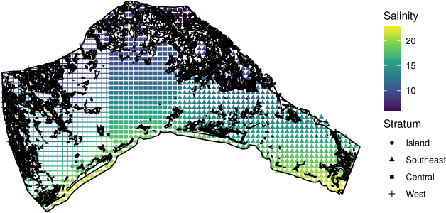
Figure 1: Barataria Bay with land (solid lines), salinity (coloured shaped points), and stratum (shapes of points).

Survey data on individuals consist of photographs of dolphin groups sighted during on-effort surveying. These data must then be parsed into a form amenable to the intended analysis framework by identifying individuals from photographs. We do not go into detail here on this process (see [12, 19]), but a key aspect is that individuals are identified by marked fins. Not all individuals in the population have a distinctive mark and marks can appear or change subtly over time. We define the marked population to be the individuals in the study that have a distinctive enough mark at some point during the survey period for it to be possible for that individual to be cataloged and resighted. In this analysis, we scale all abundance and density estimates by the proportion of marked individuals in the collection of all high-quality photographs. In this case, this proportion is $0.8$ (estimated from the data and where a preliminary study found this proportion to negligibly vary over time). We ignore uncertainty in this estimate. Therefore, reported abundance and density is for the whole population.

We assume identification of individuals is accurate and any misidentification is negligible. Once photos are identified, openSCR analysis requires organizing the sightings into their detection histories in space and time (Section 2.1.1), and a discrete approximation to the study area (Section 2.1.2) be created.

2.1.1 Defining occasions and traps

The application of SCR to this photo ID survey differs from standard applications as the detector, a boat in this case, moves in continuous space. Therefore, within the SCR framework, the encounter rate between an individual animal and the detector depends on the path the detector has taken with respect to that individual’s activity center. This can be accounted for within the standard open population SCR model by defining what is meant by a “trap” in this context and how the data are organized.

Survey data on the detector consists of GPS records, approximately every $30$ seconds, of the boat’s location whilst surveying. A survey is here defined as a single trackline traversed by the boat, usually in a single day. These surveys were grouped into a robust design [20]: secondary occasions included between 2–4 days of surveys and primary occasions contained 3–4 secondary occasions (Table 2. With respect to an openSCR analysis, the construction of secondary and primary occasions is necessary for two reasons.

Primary Occasion	Start Date
1	18-Jun-10
2	09-Nov-10
3	06-Apr-11
4	09-Jun-11
5	09-Nov-11
6	07-Feb-12
7	11-Apr-12
8	09-Apr-13
9	09-Nov-13
10	22-Apr-14
11	14-Mar-19

Table 1: Start date of each primary occasion

• Given an individual’s activity center, it is assumed that sightings of an individual are independent. This may not be true of multiple sightings of an individual close in time and so for this reason we chose to model only the first sighting of each individual within a secondary occasion and then assume first sightings over different secondary occasions are independent. We could similarly have defined secondary occasions to include a single survey each if non-independence occurred only within survey, but this leads to a large cost in computation.

• Primary occasions are so defined such that we can assume individuals do not transition between demographic states (e.g. die or emigrate) within a primary occasion and so the population changes only between primary occasions. The choice of primary occasion is thus driven by the need for this closure assumption to be reasonable.

Within each secondary occasion, we must be able to quantify the probability an individual, given their activity center, will be detected. As alluded to above, this depends on the continuous path the detector traveled. Following search-encounter methods for SCR [21], we approximate this continuous process by segmenting the boat’s path, linearly interpolating between GPS locations. We then construct a $1$km grid across the survey area and record how many surveys traversed each grid cell. We term this quantity effort. “Traps” are thus defined to be located at grid cells that have non-zero effort. Thus, conceptually, the continuous-time, continuous-space detection process is approximated by a process where detection happens instantaneously in time and contemporaneously across space within each secondary occasion. The choice of resolution for the trapping grid is a question of computational burden as a finer grid will lead to a more accurate approximation but may be computationally prohibitive.

First sightings were allocated to the trap closest to the spatial location where the sighting took place. Hence, these decisions lead to a formatted dataset where each individual is seen at most once within each secondary occasion on a single trap.

2.1.2 Mesh

In SCR, each individual is associated with a location in space: its activity center. This location is unknown and so we must average over all possible locations of that activity center. To do this we must specify a set of locations within which each individual’s activity center must reside. The extent of this spatial grid, often termed a mesh or mask, is application-specific. In this case, the mesh was constructed from a grid of $1$km grid cells within an area delineated by the bay’s barrier islands and by analysis of dolphin telemetry data collected within the bay [22]. We extended the mesh beyond the barrier islands by including a $1$ kilometer buffer area rather than truncate at the barrier islands themselves, allowing for the possibility activity centers may marginally lie outside the delineated area. We also excluded activity centers that lie on land.

The decision whether or not to exclude non-habitat, such as land, is not straightforward. The activity center is a modeling device to best explain sightings and so it is not necessary, in reality, that an individual actually ever visit its activity center. For example, in this study, it is possible an individual could be sighted on both sides of an island and so its activity center would be sensibly put in the middle of the island, on land. Despite this, however, the improved fit in the model by allowing activity centers in non-habitat is counterbalanced by the increased difficulty in interpretation. The density model in SCR refers to the density of activity centers and so it is possible that interpretation of a spatially-varying density would require one to consider high densities of activity centers for dolphins on land. Therefore, we chose to enforce that activity centers do not exist on land so that we may interpret the density surface for activity centers as a proxy for the population’s distribution.

Three spatial covariates were used in this analysis. Stratum was constructed due to prior evidence of a difference in dolphin movement between these areas [23] (Figure 1). Openness was also a constructed covariate: the bay is a highly heterogeneous habitat, especially in the north where the definition of land and water is itself changing over time. In exploratory analysis, we found that empirical encounter rates were notably higher in areas that were more sheltered from poor weather and so created the openness covariate to capture this (Supplementary Figure 1). Finally, the averaged salinity covariate quantifies the average salinity within each grid cell from Jan 2011 to Dec 2017 based on hydrodynamic modeling (Figure 1, Appendix $3$). Thus, this salinity covariate is averaged over both space and time and so can only reflect the long-term relationship between the activity center density and salinity level. Salinity levels change rapidly within the bay and so finer scale modeling would be necessary to capture the relationship between where individuals go each day and the salinity level on that day. Plots of each covariate are included in the supplementary material (Appendix $1$).

2.2 Model

The open population SCR modeling framework is described in Glennie et al. [7]. Three model components must be specified:

• detection model: the probability a sighting occurs within each secondary occasion given an individual’s activity center (Section 2.2.1);

• population dynamics model: the temporal process over primary occasions controlling when individuals are available and unavailable for detection (Section 2.2.2);

• density model: the point process model that determines where activity centers arise in space (Section 2.2.3).

2.2.1 Detection

Given an individual’s activity center $\bm{x}$, the first encounter rate with trap $j$ on primary occasion $k$ in secondary occasion $l$ is given by $e_{j,k,l}(\bm{x})=\lambda_{j,k,l}\exp\{-r_{j}(\bm{x})^{2}/(2\sigma_{j,k,l}^{2})\}$ for base encounter rate parameter $\lambda_{j,k,l}$ and encounter range $\sigma_{j,k,l}$. The function $r_{j}(\bm{x})$ is the Euclidean distance between trap $j$ and activity center $\bm{x}$. This is the well-known hazard half-normal detection model [17].

The probability of an individual being sighted on one of the $J$ traps is therefore $p_{k,l}(\bm{x})=1-\exp\left\{-E_{k,l}(\bm{x})\right\}$ where $E_{k,l}(\bm{x})=\sum_{j=1}^{J}e_{j,k,l}(\bm{x})u_{j,k,l}$ and $u_{j,k,l}$ is the effort for trap $j$ on primary occasion $k$, secondary occasion $l$. Given an individual is seen by one of the traps, the probability the sighting occurred on trap $j$ is given by the relative encounter rate $e_{j,k,l}(\bm{x})u_{j,k,l}/E_{k,l}(\bm{x})$.

Overall, the probability of a first sighting on trap $j$ in primary occasion $k$, secondary $l$ of an individual with activity center $\bm{x}$ is given by $p_{k,l}(\bm{x})e_{j,k,l}(\bm{x})u_{j,k,l}/E_{k,l}(\bm{x})$. This is known as the competing hazards detection model [17].

2.2.2 Population dynamics

Whether an individual is available for detection or not during a primary occasion depends on its state. In Glennie et al. [7], individuals have three states (“unborn”, “alive”, and “dead”) and are only available for detection in one of them (“alive”). Individuals change states between primary occasions and not within (see closure assumption discussed above).

It is important to remember that these states are inferred from an individual’s detection availability and not from observed life events. Conceptually, each individual’s encounter history is explained by a possible period of no sightings (“before” they become available for detection), a mix of sightings and no sightings coherent with the detection process (“during”) and then possibly a period of no further sightings (“after” being available). We wish to estimate the probability between two consecutive primary occasions that an individual transitions from one of these states to the next.

We will specify three states for this temporal process and name them “before” ($B$), “during” ($D$), and “after” ($A$). Furthermore, we will enforce that individuals must begin in primary occasion $1$ in either state $B$ or $D$ and then proceed through the states in the sequence $B\rightarrow D\rightarrow A$ until all individuals reach state $D$ or $A$ by the end of the survey.

The reason this state process is so defined is by analogy with population dynamics: individuals enter a population by immigration or being born (or in this study entering the marked population), live for some period where they may be detected, and then emigrate or die. It is through this analogy that the probability of the transition $B\rightarrow D$ is called recruitment probability and $D\rightarrow A$ survival probability. For survival probability it is well known that estimates can be biased by unmodeled heterogeneity or emigration [8, 11, 24] and so it is often termed apparent survival. Though emigration may be the most important factor, it is only one of many possible reasons that the transition probability $D\rightarrow A$ may be a biased estimate of true survival probability. A similar argument leads one to question interpretation of transitions $B\rightarrow D$ as solely recruitment. Overall, we must recognize that the model as specified simply clusters encounter histories in time so as to best describe what was observed and we must then, as a secondary step, carefully interpret this clustering in terms of population dynamics.

For this application, we define both the survival and recruitment processes in continuous time. Let $\phi_{k}^{\delta_{k}}$ be the probability of the transition $D\rightarrow A$ between primary occasions $k$ an $k+1$ where $\delta_{k}$ is the time between the mid-points of both occasions.

For transitions $B\rightarrow D$, we specify a different parameterisation from Glennie et al. [7] to allow for irregular gaps between primary occasions. Let $\gamma_{k}$ be the transition rate between primary occasions $k$ and $k+1$ and $\beta_{k}$ the probability of the transition between these primaries. We define $\beta_{1}=\exp\left(-\sum_{k=1}^{K-1}\gamma_{k}\delta_{k}\right)$ and $\beta_{k}=(1-\beta_{1})\gamma_{k}\delta_{k}/\sum_{m=1}^{K-1}\gamma_{m}\delta_{m}$ for primary occasion $k>1$.

2.2.3 Density

We do not directly model the density of individuals in the population at any particular time: we model the density of activity centers for individuals alive at some point during the survey. This is a point pattern in space and does not depend on time. We assume activity centers arise from an inhomogeneous Poisson process with intensity $D(\bm{x})$ at location $\bm{x}$ [17]. Defining $\overline{D}$ as the mean value of $D$ over the study region, this implies that the probability density of an activity center occurring at location x is $D(\bm{x})/\overline{D}$ and the total number of expected activity centers is $\overline{N}=\overline{D}A$ where $A$ is the area of the study region [25].

Density and abundance for any given time and location is derived jointly from the population dynamics and density models. Defining $D_{k}(\bm{x})$ to be the density during primary occasion $k$ at location $\bm{x}$, we have that $D_{1}(\bm{x})=\beta_{1}D(\bm{x})$ and that for $k>1$, $D_{k}(\bm{x})=\phi_{k-1}^{\delta_{k-1}}D_{k-1}(\bm{x})+\beta_{k}D(\bm{x})$.

For this application we assume population dynamics do not vary over space therefore the population’s distribution has the same spatial pattern over the entire survey period and only the magnitude of the density changes over time.

2.2.4 Fitting the model

Given the three components of the model specified above, the likelihood can be stated (see [7]) and we can compute maximum likelihood estimates for the parameters. We fit all models in the R package openpopscr (available at https://github.com/r-glennie/openpopscr). There are two important computational details to refer to here. First, all parameters were transformed to a working scale with log (for strictly positive parameters) or logit (for parameters that are probabilities) link functions. Second, transformed parameters could be represented by a linear predictor to allow for linear or semi-parametric covariate effects. Semi-parametric effects were specified using thin plate regression splines [26] with fixed degrees of freedom. Semi-parametric effects were considered to allow some parameters to vary over averaged salinity, time, and space. In particular, we restricted attention to models where $\lambda,\sigma$ could depend on stratum, openness, and time; $\phi,\beta$ could depend on time; and $D$ could depend on spatial location and average salinity. What covariate effects to consider on each parameter is a decision the analyst must make given the existing knowledge of the population and the surveys [27].

2.2.5 Model Selection

Models were selected using Akaike’s information criterion (AIC) [28]. The decision on whether or not to include a covariate effect on a given parameter was made using AIC. A sequential model selection strategy was used in this case: first covariate effects on detection process parameters was performed, then effects on the survival parameters, and finally on the density surface. The degrees of freedom for included regression splines were selected by AIC up to a maximum (set by what was computationally and numerically feasible). For one-dimensional smooths, the maximum was $10$ and for two-dimensional smooths the maximum was $20$.

We term the set of degrees of freedom for all smooths specified in a model to be that model’s smoothing parameters. In the case where two or more models had an AIC score less than two units from the model with the minimum AIC, then the smoothing parameters from all such models were retained to form a candidate set of smoothing parameters. Model selection then continued with smoothing parameters from the model with the minimum AIC until the final model with best AIC was determined. This final model was then re-fit with each set of smoothing parameters in the candidate set to form a final set of models. Inference would then take into account uncertainty in parameters and in the smoothness of regression splines across equally supported models.

2.2.6 Inference

For a single fitted model, the maximum likelihood estimators were assumed to follow an asymptotic normal distribution. The variance-covariance matrix for this asymptotic distribution was estimated by the inverse Hessian [29]. The maximum likelihood estimates from each model, however, are on the link scale; furthermore, they do not include derived estimates such as the density and abundance within each primary occasion. In this case, the uncertainty in the estimates on the scale meaningful for inference was determined by parametric bootstrap from the asymptotic distribution of the maximum likelihood estimators [30].

When more than one model was selected to be in the final set (due to uncertainty in smoothing parameters), model-averaged parameter estimates and uncertainty in these estimates were approximated by repeating the following algorithm a large number of times:

1. For $M$ final models, sample an integer from the set $\{1,\ldots,M\}$ where the probability of selecting integer $m$ (i.e. model $m$) is given by $w_{m}/\sum_{i=1}^{M}w_{i}$ where $w_{i}$ is the AIC weight [27] for model $i$.

2. Given a selected model $m$, simulate parameters on the working scale using the maximum likelihood estimates and estimated variance-covariance matrix from model $m$, assuming the asymptotic normal distribution for maximum likelihood estimators.

3. Convert these simulated parameters on the working scale to the scale meaningful for inference.

Given the above steps are repeated a large number of times, the model-averaged point estimate for each parameter is simply the mean over all simulations. Uncertainty in these estimates can be quantified with the $95\%$ confidence interval, approximated by the $2.5\%$ and $97.5\%$ quantiles of the simulated parameter estimates. Furthermore, estimates for derived quantities can be computed from the bootstrap samples.

2.2.7 Goodness-of-fit

Goodness-of-fit was assessed by comparing data simulated given our inferred parameters with the observed data. To simulate comparable data, we first sampled parameters from the bootstrap samples. Given these parameters, data was simulated assuming the same detector paths were surveyed.

To compare the simulated data with the observed, we conducted three randomization tests [30] with the intention of testing the goodness-of-fit with respect to each of the model’s components. The statistic for each test was as follows:

• Test 1 (Testing Recruitment): the number of individuals seen for the first time on each primary occasion;

• Test 2 (Testing Survival): the average number of primaries between the first and last sighting of an individual;

• Test 3 (Testing Density): the number of individuals detected on each trap over the entire survey period.

3 Results

Surveys were collected into $34$ secondary occasions lasting on average $5$ days each. These were then organized into $11$ primary occasions. Time between primary occasions was irregular with approximately $0.5$ years between primary occasions, except for the last primary occasion which notably occurred approximately $5$ years after primary occasion $10$ (Appendix 2).

In total, 2091 unique individuals were sighted during the entire survey period over a constructed grid of $909$ traps. Along with a constructed mesh of 1284 points, this comprises a large dataset given the computational and computer memory demands of fitting open population SCR models.

Figure 2 shows the traps surveyed and the number of individuals sighted for the first time ($u$) in each primary occasion. These two aspects of the data highlight an important point: the inference drawn from the analysis must be considered in light of the spatial and temporal irregularity in the data. The southeast was surveyed only in primary occasion $11$ and so is likely treated as equivalent to outside the study area for inferences made in primaries $1$–$10$. Similarly, many individuals were seen for the first time in primary $11$ (and most in the southeast) and so there is no new temporal information on the survival rates of these most recent individuals; the inferences made on survival stem from recaptures in primary occasion $11$ of those individuals seen in primaries surveyed five years earlier, which covered a subset of the study area.

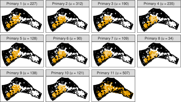
Figure 2: Surveyed traps (yellow points) and non-habitat (black points) for each primary occasion (1–11) and, in brackets, number of individuals $u$ seen for first time.

3.1 Model Selection

Model selection using AIC was successful when determining whether or not to include factor covariate effects (e.g. stratum) on parameters. AIC discriminated poorly between models with different degrees of freedom on regression splines (Appendix 3). This manifested in two ways.

For survival and recruitment, there was clear support for temporal variation, but uncertainty when using AIC to select how smooth the temporal relationships were, leading to six models with AIC scores within two units of the minimum AIC score (Appendix 3, Table 3). The concern here is that these models lead to qualitatively different interpretations of how survival changed over time (Section 3.3). Thus, model averaging was used across these six top models.

For density, AIC provided clear support for an optimal degrees of freedom for a regression spline on averaged salinity; however, AIC failed to lend support for any degree of freedom less than the maximum degrees of freedom that was computationally feasible for the $(x,y)$ regression spline on density. Further to this, support for further increasing the degrees of freedom was driven by improved fit near the central passes around the islands and not from an overall improved fit over the study area. This inability to identify an optimal smoothness is either due to AIC being a sub-optimal criterion (as the penalization for degrees-of-freedom is fixed) [31] or due to model misspecification. In particular, the inhomogeneous Poisson process and smoothness assumption for the mean density surface may both be violated by unmodeled clustering of activity centers in space or a spatially-varying smoothness.

Ultimately, the candidate set of models selected on which to base inference had the form:

$$\lambda \sim\text{stratum}+\text{openness}+\text{primary occasion}$$

$$\sigma \sim\text{stratum}+\text{openness}+\text{primary occasion}$$

$$\gamma \sim s(\text{time},\text{df}=a)$$

$$\phi \sim s(\text{time},\text{df}=b)$$

$$D \sim s(x,y,\text{df}=20)+s(\text{averaged salinity},\text{df}=5)$$

where $\sim$ denotes that the working parameter corresponding to the parameter on the left-hand side had covariate effects for those covariates on the right-hand side. The $s$ symbol indicates a regression spline was used and df gives its degrees of freedom. Models had degrees of freedom $(a,b)$ in the set $\{(6,3),(7,3),(6,4),(6,5),(7,4),(7,5)\}$.

We now review the results obtained from $10,000$ simulations from the model-averaging bootstrap (Section 2.2.6) of these six models.

3.2 Detection

Base encounter rate $\lambda$ and encounter range $\sigma$ varied by primary occasion (as a factor covariate), stratum, and openness. In particular, encounter range was similar across most primary occasions ($3502$; $95\%$ CI: $2737$–$4061$) with the exception of primary occasion $8$ where encounter range was substantially reduced, coinciding with poor weather that also affected survey effort (Appendix 4).

3.3 Survival

Estimated survival probability (Figure 3) initially increases from primary occasion $1$ until primary occasion $4$ and then more gradually decreases until primary occasion $11$. Discrepancy between the different possible temporal regression splines on survival is largest around the initial increase in survival with more smooth models predicting a less rapid increase compared to those with higher degrees of freedom (Appendix 5).

Figure 3: Mean survival probability estimates ($\phi$) and approximate $95\%$ confidence interval over primary occasion from $10000$ model-averaging bootstrap samples along with mean survival probability estimates from contributing models with three (squares), four (triangles), and five (diamonds) degrees of freedom.

3.4 Recruitment

Recruitment had a consistent pattern across models in the candidate set. Recall recruitment here refers to the number of individuals that make the transition $\text{B}\rightarrow\text{D}$. Therefore, recruits can refer to any event that causes an individual to become available for detection, e.g., moving from peripheral habitat into the surveyed area or becoming a member of the marked population. Recruitment is relatively high immediately after the oil spill (Figure 4) and then steadily decreases prior to $2014$ when a short increase in recruitment occurs. Recruitment is then estimated to be relatively low in the five years prior to the $2019$ surveys.

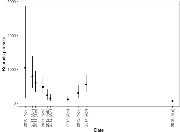
Figure 4: Mean estimated number of recruits per year between primary occasions and approximate $95\%$ confidence interval from $10000$ model-averaging bootstrap samples.

3.5 Density

The estimated density surface depends on a one-dimensional regression spline of averaged salinity and a two-dimensional spatial smooth. For the spatial smooth, as AIC failed to identify an optimal smoothness, the maximum degrees of freedom that were computationally feasible were used ($k=20$). Recall also we assume a constant distribution over time as we do not model variation in this pattern through spatially-varying population dynamics.

The estimated mean density is heterogeneous across the study area with high density around the islands and passes between the bay and the gulf (Figure 5). Further locations of higher than average density occur in the central area of the study region and the northeast near the leveed banks of the Mississippi river. Overall, mean density is lower in the southeastern region of the study area compared to the west and central areas.

Two difficulties with fitting and interpreting this density surface model can be appreciated by considering the higher densities predicted in the extreme north of the study area and in the area south of the islands, outside the bay.

• No survey lines extended to the extreme north and there is limited information on any individuals that would reside there given the estimated activity range of the animals, thus the density surface is unconstrained by the data in this area leading to a high degree of uncertainty. We quantify uncertainty by the inter-quartile coefficient of dispersion (IQD) over the bootstrap samples (Figure 6) and observe high uncertainty in the north. The difficulty is that if this region of high uncertainty is included in inference on abundance then uncertainty in abundance will be excessive compared to what we could say if we restricted our inference to a smaller region. For this reason, we re-defined the study area to be those locations where $\text{IQD}<0.95$, excluding those areas where uncertainty was excessively high. We will term the area of those points where $\text{IQD}<0.95$ to be the region of inference. Appendix 6 contains more details on delimiting this region and on why IQD was used over another popular choice: coefficient of variation.

• In the south, density appears to increase rapidly close to the islands, especially in the central part of the island stratum. This raises a difficulty when one reflects on how the mesh was constructed. We used a one kilometer buffer beyond the islands to account for individuals whose activity would be coherent with an activity center outside the bay; however, in retrospect, if this buffer were extended then the inference would be to extend this increase in density indefinitely (as there is no survey effort beyond this area). Therefore, the choice of buffer would have a substantial impact on the abundance estimated. In this case we chose to restrict individuals to this area and so take abundance as including those individuals in the one kilometer buffer beyond the islands, but no more, appealing to available telemetry data indicative of dolphin habitat [22].

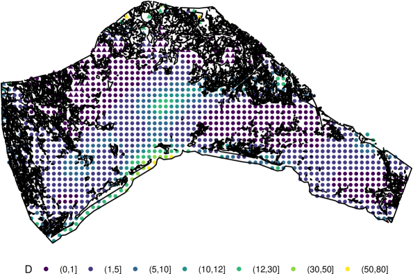
Figure 5: Estimated mean density $D$ (individuals per square kilometer) from $10000$ model-averaging bootstrap samples. Triangles are mesh points excluded from region of inference.

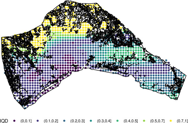
Figure 6: Estimated inter-quartile dispersion coefficient (IQD) for density from $10000$ model-averaging bootstrap samples.

3.6 Salinity

Density also depended on a simple regression spline of averaged salinity from $2011$–$2017$. As spatial location and salinity are correlated in the Bay, it is challenging to separate the salinity effect from the spatial effect. A common approach would be to consider the effect salinity has on density conditional on a given spatial location; however, this does not address the interest we have in this effect. We are interested in the population’s distribution with respect to salinity. For this reason, we interpret the salinity effect using the mean density and abundance of individuals with activity centers within (binned) salinity bands (Figure 7). It is important to consider both density and abundance as the spatial area corresponding to each salinity band is different. Density is higher in higher salinity bands, but still a large abundance of activity centers occur in lower salinity bands between $12$–$17$ ppt.

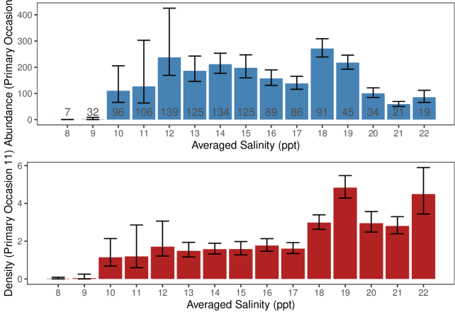
Figure 7: Estimated density (individuals per square kilometer), bottom panel, and abundance, top panel, in primary occasion $11$ in each salinity (ppt) band (where a salinity band with label $x$ includes all mesh points with salinities in the interval $[x-0.5,x+0.5)$) from $10000$ model-averaging bootstrap samples with approximate $95\%$ confidence intervals. Numbers at base of each bar in top panel is the area (in square kilometers) covered by each salinity band. Recall that population distribution does not change over time, so the patterns above will be the same for other primary occasions.

3.7 Abundance

Abundance within the region of inference initially increases from $\sim 2200$ in primary occasion $1$ (Jun $2010$) to $\sim 3000$ in primary occasion $5$ (Nov $2011$), then approximately varies around $\sim 3000$ up to primary occasion $10$ (Apr $2014$), before declining substantially to $\sim 2100$ in primary occasion $11$ (Mar $2019$) (Figure 8).

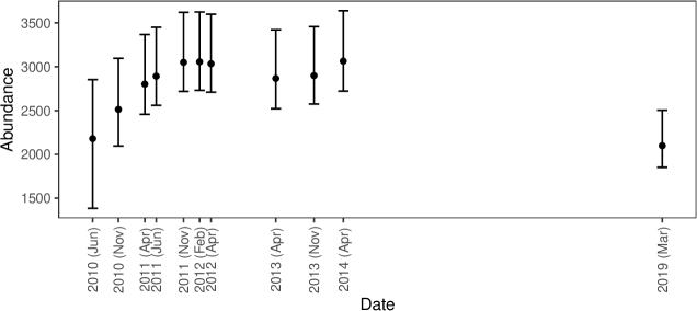
Figure 8: Estimated mean abundance for each primary occasion with approximate $95\%$ confidence interval (vertical lines) from $10000$ model-averaging bootstrap samples

3.8 Goodness-of-fit

Goodness-of-fit tests showed evidence of good and poor fit to different aspects of the data (Figure 9).

The expected number of new individuals sighted, $u$, for each primary occasion was well described for most primary occasions besides primary occasions $8$ and $11$ where the model over and under predicted recruitment respectively, indicating a lack of ability in the model to capture extreme changes in recruitment that both of these primaries may have experienced.

The observed and expected mean time between first and last sighting of an individual ($\text{t}_{\text{between}}$) gave no evidence of poor model fit.

The number of individuals sighted on each trap within each stratum indicated adequate model fit except the island stratum where there is evidence the model underestimates either density or encounter rate. Given separate detection parameters are estimated for each stratum, a plausible assumption is that this indicates poor density model fit and this coincides with the issues discussed above when determining the smoothness of the density surface.

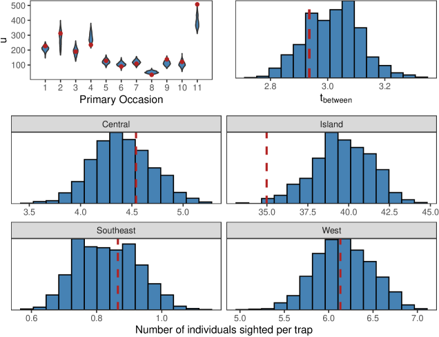
Figure 9: Goodness-of-fit tests: (top-left) distribution of the simulated number of individuals seen for the first time (blue violin) for each primary occasion; (top-right) distribution of mean time between first and last sighting of an individual; (bottom) distribution of mean number of individuals sighted per trap in each spatial stratum. All distributions are derived from $1000$ simulated datasets; solid points and dashed lines give the corresponding statistic computed from the observed data.

4 Discussion

In this final section, we complete our description of the analysis workflow for this case study (Section 4.1), discuss the limitations of this analysis (Section 4.2), and the opportunity for future research (Section 4.3).

4.1 Case Study

The workflow presented for this case study has taken the following route: (1) put the data and survey into an openSCR context by defining occasions, traps, and a mesh; (2) specify the three components of the model: detection, population dynamics, and density; (3) determine the set of models to be considered, including possible covariate effects; (4) select between these models using a suitable approach (e.g. AIC) and create a final set of candidate models that are negligibly discriminated between; (5) simulate parameter estimates and derived quantities from a model-averaging parametric bootstrap; (6) assess goodness-of-fit to identify limitations. We then presented the results from this analysis (Section 3). The final stage is to interpret these results and consider how they are related to changes in the population.

The exploision and subsequent sinking of the Deepwater Horizon drilling rig occurred in late April 2010 and by early June oil had reached the shores of all five Gulf coast states. The photo-ID surveys did not begin until 26 June and so we do not have information on the population size prior to the spill. For the first two years post-spill, abundance steadily increases (Figure 8). Over the same time period, survival probability is initially low (compared to similar dolphin populations where annual survival $\approx 0.95$ [32, 33]) and then increases (Figure 3); recruitment rate decreases but is relatively high over this period (Figure 4). Together, this inference is coherent with individuals entering the study area who contribute to a higher survival rate compared to those present in the study area immediately post-spill. These recruits could be from outside the study area or could be individuals present in the surveyed area that acquire marks. This is the first example of how interpretation must be made in light of the model assumptions and how the data were collected. Prior to $2019$, the southeast stratum was not surveyed and so individuals in this area prior to $2019$ are likely to remain undetected. This means that if individuals in this stratum had moved into other strata prior to $2019$, the model would capture this through the recruitment process and so before $2019$ the southeast stratum should be treated, when interpreting inference, as also outside the study area. In other words, the high recruitment could reflect a redistribution of individuals within the bay where individuals in peripheral habitat replace those in island, central, and west strata who were subject to high mortality.

Between $2012$ and $2014$, abundance appears relatively stable (Figure 8). Survival probability decreases from $2012$ and appears to remain stable afterward with a mean $\sim 0.9$ (Figure 3). This mortality does not affect abundance substantially despite relatively low recruitment between $2012$–$2014$ until an estimated increase in recruitment at the beginning of $2014$ (Figure 4). The reason for this increase in recruitment is not clear from the model: it could possibly reflect further redistribution of individuals within the bay, increased attribution of marks, or changes in prey distribution or fishing leading to new individuals entering the population. Overall, the inference can be interpreted in terms of change observed in the study: the population continues to experience higher mortality than expected for comparative dolphin populations and abundance does not reflect this substantially due to a subsequent increase in new individuals entering the surveyed area, an area that itself shifts in definition over primary occasions.

Finally, during the $5$ years between the survey in $2014$ and new surveys in $2019$, inference clearly points to a population where recruitment is low and survival remains at its previous level, leading to decline in population abundance (Figure 8).

Together with these temporal inferences, density surface estimation allows us to infer where in the bay these events have most impact. Using activity centers as a proxy for population distribution, it is clear that individuals spend much of their time around the islands and in particular near the passes between the islands (Figure 5). This is likely due to the increased availability of prey and ease of access between the bay and the gulf [22]. There are however other areas where density is estimated to be higher than average in the northeast near the Mississippi river and in the center of the central stratum. Similarly, we can interpret the population’s distribution with respect to average salinity: density is higher in higher salinity ($>19$ ppt), corresponding with their preference for area around the islands, but still a large portion of the population have activity centers in lower salinity around $12$–$18$ ppt.

4.2 Limitations

Here, we discuss the limitations of the analysis given the assumed model structure. In Section 4.3 we consider future extensions to the model itself.

The case study highlighted four key limitations when using the proposed openSCR method to make inference:

• Sensitivity of inference to model selection: Selecting between survival models with different degrees of freedom led to substantially different inference on how survival varied over time. When assessing the impact of the oil spill, a justified estimate of survival in the first year post-spill is an important quantity [15], and the sensitivity of this estimate to the smoothness of the underlying regression spline is therefore an important limitation to consider. Estimating a separate survival probability for each interval between primaries would remove the need to consider estimating smoothing parameters, however, such models would surrender the chance to borrow strength across primaries with similar survival estimates, be difficult to fit due to poorer parameter identifiability [34], and would further increase computational burden. Model-averaging, as implemented here, is taken as the most cautious approach as it incorporates the parameter sensitivity into the overall parameter uncertainty.

• Estimating smoothness: Related to the previous limitation, using AIC to select smoothness of regression splines is known to be a sub-optimal strategy in traditional smoothing spline applications and so it is possible similar limitations exist when using it in this context. By limiting the degrees of freedom as we did here, we likely oversmoothed density in areas were sharp changes exist, which is supported by the identified lack of fit in these areas.

• Delimiting a region of inference: the thin plate regression splines used here are unreliable when extrapolating beyond the domain informed by the data [35]. In regression contexts, this can be prevented as this domain is (partially) observable, while in SCR it is typically unknown a priori over what area inference can be confidently applied as this depends on the activity of the animals. Therefore, it is likely that one will try to infer density in regions with no support from the data and so completely informed by assumed behaviour of the spline, which in this case study extrapolates observed trends at the boundary of the region informed by the data. Here, we used the uncertainty on these estimates to define the region a posteriori within which we based our inferences.

• Interpretation: Despite the conceptual correspondence between openSCR models and the population’s dynamics, it is challenging to interpret inference as it is necessary to consider the cause of observed clusters in capture histories of detections and non-detections. In this case study, we use the inference from the models and qualitative understanding of the biology and context of the population in order to make an informed interpretation of the results. Without incorporation of observed recruitment, mortality, or movement events, it is not possible to elicit these interpretations from the quantitative model alone as more than one possible cause can produce the observed structure in capture histories.

These limitations do not preclude drawing inference, as we show in the case study, but they are important practical obstacles that practitioners will likely face with similar applications.

4.3 Research Opportunities

Our proposed workflow focuses on what is currently feasible when applying openSCR to large datasets. Data collected over long time periods and over large populations will, however, likely provide the opportunity to infer more about populations using openSCR and motivate the need for more realistic model components to be added. There are clear opportunities for future research: (1) improve the computational efficiency of the current methods; (2) estimate smoothness of density surfaces by shrinkage methods in a penalized likelihood framework rather than by the stepwise AIC model selection used here [36]; (3) incorporate further individual heterogeneity by discrete or continuous random effects, e.g., to capture those individuals affected more by the spill and so having higher mortality [37]; (4) account for non-Euclidean distances in detection models, e.g., it is possible individuals move up and down the coast of islands not coherent with the pattern expected under the detection model [38]; (5) remove the need to discretize the continuous-space, continuous-time detection process in the boat-based photo-ID survey to remove unnecessary trap construction and build a more realistic model of the detection process; (6) fit spatio-temporal population dynamics models where survival and recruitment can vary over space, allowing for density surfaces for each primary occasion to vary, and attempt to capture redistribution of the population over time.

5 Conclusions

This case study shows that it is feasible to draw complex inference on spatially-varying density and time-varying population dynamics from large, long-term, capture-recapture studies. As computational and statistical methods continue to develop, openSCR will become an attractive method for drawing these inferences. This requires practitioners to discuss how these methods perform and for attention to be drawn to future methodological challenges. The workflow presented above provides a guide for practitioners to follow and adapt when applying these methods; the limitations highlighted during the application points researchers toward future methods development.

Appendix 1: Covariates

The analysis included the following possible covariates: time, stratum, openness, average salinity, and $(x,y)$ location. Time refers to the time at which each primary occasion took place measured in years. The other three covariates are spatial variables: the first two are intended to explain variation in detectability across traps and average salinity with $(x,y)$ is intended to explain variation in density of activity centers. Stratum was defined as a categorical variable that separated spatial regions that may have had different sighting rates (Figure 10).

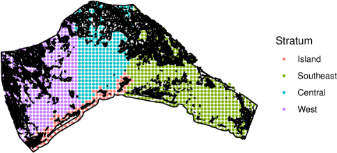
Figure 10: Strata

Openness is another categorical variable used to capture the relatively open and sheltered parts of the bay (Figure 11).

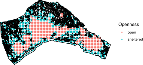
Figure 11: Openness

Finally, average salinity is a continuous spatial covariate. To compute the average salinity covariate, first the salinity over a $10$ meter grid was averaged over time from Jan $2011$ to Dec $2017$. The average salinity associated with each mesh point is then the spatial-average of this time-averaged salinity within one kilometer of the mesh point. Ultimately, the salinity covariate is averaged across both time and space. Henceforth, the term averaged salinity will refer to this covariate. Figure 12 shows the computed averaged salinity.

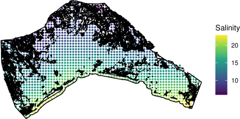
Figure 12: Salinity averaged over $7$ years ($2011$–$2017$) and over a one kilometer grid

Appendix 2: Occasions

The photo-ID surveys are first grouped into 34 secondary occasions and then secondary occasions are grouped into 11 primary occasions. Each primary occasion contained $3$ secondary occasions, except the final primary which contained $4$. On average, each secondary occasion contains $5$ tracks. Table 2 gives the start date of each primary occasion.

Primary	Start Date
1	18-Jun-10
2	09-Nov-10
3	06-Apr-11
4	09-Jun-11
5	09-Nov-11
6	07-Feb-12
7	11-Apr-12
8	09-Apr-13
9	09-Nov-13
10	22-Apr-14
11	14-Mar-19

Table 2: Start date of each primary occasion

The time between primary occasions (which is important for scaling the relevant population dynamics, i.e., survival over one year is different from survival over two months) was computed as the time between the mid-points of each primary occasion given in units of years in Table 2.

Interval	Duration
1–2	0.4
2–3	0.4
3–4	0.2
4–5	0.4
5–6	0.2
6–7	0.2
7–8	1.0
8–9	0.6
9–10	0.4
10–11	4.9

Table 3: Time interval (in years and rounded to one decimal place) between primary occasions

Appendix 3: Model Selection

Recruitment and survival both depended on regression splines of time whose degrees of freedom where selected by AIC. The optimal model was found by optimizing the AIC using a method of steepest descent. Table 4 shows the $\Delta$AIC values for $10$ models with the lowest AIC’s fitted when determining the degrees of freedom for these splines. The smoothing parameters for models with $\Delta$AIC $<2$ were taken as part of the candidate set of smoothing parameters over which to fit the final selected model.

Recruitment df	Survival df	$\Delta$AIC
6	3	0.0
7	3	0.5
6	4	0.6
6	5	0.9
7	4	1.1
7	5	1.4
6	6	2.6
6	7	2.9
7	6	3.1
5	3	3.2

Table 4: $\Delta$AIC (difference between AIC for that model and the AIC for the optimal model) for best 10 models fitted when determining the degrees of freedom (df) in time-varying population dynamics parameters, survival and recruitment

The density surface was selected to depend on regression splines of both spatial location $(x,y)$ and averaged salinity. A maximum was set on the degrees of freedom of both splines of $10$ and $20$ knots respectively. In the case of salinity, AIC clearly selected $5$ degrees of freedom as optimal, while for spatial location, the AIC selected the maximum degrees of freedom.

Appendix 4: Detection Process

Base encounter rate varied over time without any clear pattern (Figure 13), likely driven primarily by survey conditions.

Encounter range was similar across most primary occasions (Figure 13) with a mean of $3502$ ($2737$–$4061$) with the notable exception of primary $8$ where encounter range was significantly lower. Recall that these estimates are not derived from a regression spline and so any smooth pattern is induced by the data.

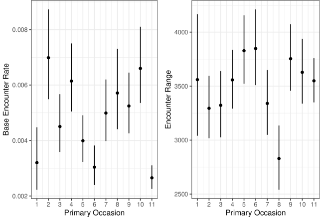
Figure 13: Mean detection parameter estimates ($\lambda,\sigma$) and approximate $95\%$ confidence interval over primary occasions (1–11) from $10000$ parametric (model-averaging) bootstrap resamples

Comparing strata, it is best to interpret the base encounter rate and the encounter range jointly (Figure 14). For the Island stratum, base encounter rate is much higher than in other strata, while encounter range is slightly smaller: the reduced encounter range could simply be due to the relatively small extent of the island stratum compared to other strata, while the enlarged base encounter rate suggests an increased encounter rate within the island stratum compared to surveying that takes place in other strata. The other notable stratum is the Central stratum. In the Central stratum, the encounter range is substantially larger while the base encounter rate is much smaller which suggests that individuals move (or are detectable) over a larger area around their activity center but that the encounter rate is lower compared to other strata.

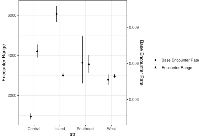
Figure 14: Mean detection parameter estimates ($\lambda,\sigma$) and approximate $95\%$ confidence interval for each stratum from $10000$ parametric (model-averaging) bootstrap resamples

There was no significant difference between encounter range in the open and sheltered parts of the study area; however, there was a substantial and significant difference in base encounter rate. Encounter rate for surveying in the open was lower than in the sheltered (open: $0.0025$ ($0.0021$–$0.0031$), sheltered: $0.0067$ ($0.0057$–$0.0079$)). This could either be due to different behavior of the dolphins in these two areas leading to disparity in detection or, and perhaps more likely, is that detection probability is higher in sheltered areas.

Appendix 5: Survival

Mean estimated survival probability initially increases from primary $1$ until primary $4$ and then approximately decreases from then until primary $11$ (Table 5). We ascribe each estimated survival probability to the mid-point of the primary occasion preceding the interval to which the survival probability pertains, e.g. the survival probability for primary $1$, whose mid-date is 9 Nov 2010, is the probability of an individual surviving the interval between primary $1$ and primary $2$. In reality, these estimates refer to the survival probability over this interval and the simplest assumption is to assume survival probability is constant between primaries.

Date	$\phi$	LCL	UCL
09-Nov-10	0.82	0.70	0.91
06-Apr-11	0.89	0.85	0.93
09-Jun-11	0.92	0.88	0.96
09-Nov-11	0.92	0.89	0.96
07-Feb-12	0.91	0.89	0.94
11-Apr-12	0.90	0.86	0.93
09-Apr-13	0.90	0.85	0.93
09-Nov-13	0.89	0.82	0.94
22-Apr-14	0.89	0.84	0.94
14-Mar-19	0.88	0.86	0.90

Table 5: Mean survival probability estimates ($\phi$) and approximate $95\%$ confidence interval (LCL, UCL) over primary occasion from $10000$ parametric (model-averaging) bootstrap resamples

Appendix 6: Determining the region of inference

Figure 15 shows the mean estimated density for the marked population (including effects of both spatial location and averaged salinity). There are two important facets of the modeling.

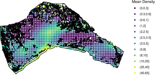
Figure 15: Estimated mean density for marked population from $10000$ parametric (model-averaging) bootstrap resamples

We use the estimated uncertainty in the density surface to demarcate the area of inference. It is not sensible to use the standard deviation to do this as estimated density has, in theory, a log-normal asymptotic distribution and so the estimated standard deviation is proportional to the estimated mean. A popular measure of uncertainty than accounts for this is the coefficient of variation (CV): the standard deviation divided by the mean. In this case, however, the CV poorly describes the uncertainty in the density surface (Figure 16): this is because the density estimator has a heavily skewed distribution and so both the mean and standard deviation poorly reflect the center and spread of the distribution respectively. Thus, in the far north CV is low because mean and standard deviation are both extremely large due to the skewness being eventuated when uncertainty is larger.

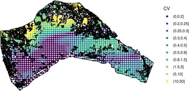
Figure 16: Estimated coefficient of variation (CV) for density from $10000$ parametric (model-averaging) bootstrap resamples

Thus, as an alternative, we use the interquartile coefficient of dispersion, defined as the interquartile range divided by the median (Figure 17). As this is based upon quartiles of the estimator’s distribution, skew and outliers have less effect.

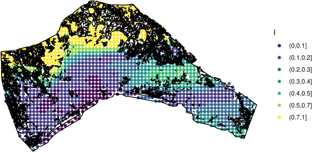
Figure 17: Estimated inter-quartile coefficient of dispersion (I) from $10000$ parametric (model-averaging) bootstrap resamples

The region of inference can now be defined based on a threshold of this estimated uncertainty. In the results presented in the main paper, a threshold of $0.95$ was selected, which truncated approximately $10\%$ of the spatial locations from the original mesh as shown in Figure 18.

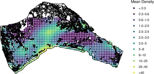
Figure 18: Estimated mean density for marked population from $10000$ parametric (model-averaging) bootstrap resamples

Appendix 7 : Salinity hydrodynamic modelling details

Salinity estimates were from the Delft3D-based hydrodynamic model described by White et al. [39] and Takeshita et al. [40]. The model performed historical simulations to estimate salinity conditions from 2011 to 2017 in the Barataria Basin. It was calibrated and validated using a collection of field observations, including salinity, by comparing model output with data from USGS, CRMS, and NOAA. The model used field measurements (e.g., river discharge and tides) to impose boundary conditions and atmospheric forces for those specific years. The Delft3D model uses a 375 m resolution triangular grid in the majority of our study area, but near the Mississippi River, a small area of our modeled estimates has a 125 m resolution. Within the model, salinity estimates are depth averaged. We used publicly available packages (sf, stars, raster, and akima) for the statistical software R (version 4.0.0) to generate the estimated salinity averages by interpolating the daily triangular Delft3D model output into a 375 m square grid and removing pixels that had no water (i.e., were all land). We then averaged the salinity estimates in each cell across the entire available timeframe for estimates from Barataria Basin (January 2011 to December 2017) to generate a single spatial snapshot of average salinities across the basin for the multi-year time period.

References

- Seber and Schofield [2019] George A. F. Seber and Matthew R. Schofield. Capture-recapture: Parameter estimation for open animal populations. Springer, 2019.
- Jolly [1965] George M. Jolly. Explicit estimates from capture-recapture data with both death and immigration-stochastic model. Biometrika, 52(1/2):225–247, 1965.
- Schwarz and Arnason [1996] Carl J. Schwarz and A. Neil Arnason. A general methodology for the analysis of capture-recapture experiments in open populations. Biometrics, 52(3):860–873, 1996.
- Cormack [1964] Richard M. Cormack. Estimates of survival from the sighting of marked animals. Biometrika, 51(3/4):429–438, 1964.
- Williams et al. [2002] Byron K. Williams, James D. Nichols, and Michael J. Conroy. Analysis and management of animal populations. Academic Press, 2002.
- Gardner et al. [2010] Beth Gardner, Juan Reppucci, Mauro Lucherini, and J. Andrew Royle. Spatially explicit inference for open populations: estimating demographic parameters from camera-trap studies. Ecology, 91(11):3376–3383, 2010.
- Glennie et al. [2019] Richard Glennie, David L. Borchers, Matthew Murchie, Bart J. Harmsen, and Rebecca J. Foster. Open population maximum likelihood spatial capture-recapture. Biometrics, 75(4):1345–1355, 2019.
- Efford and Schofield [2020] Murray G. Efford and Matthew R. Schofield. A spatial open-population capture-recapture model. Biometrics, 76(2):392–402, 2020.
- Turek et al. [2021] Daniel Turek, Cyril Milleret, Torbjørn Ergon, Henrik Brøseth, Pierre Dupont, Richard Bischof, and Perry De Valpine. Efficient estimation of large-scale spatial capture–recapture models. Ecosphere, 12(2):e03385, 2021.
- Gardner et al. [2018] Beth Gardner, Rahel Sollmann, N. Samba Kumar, Devcharan Jathanna, and K. Ullas Karanth. State space and movement specification in open population spatial capture–recapture models. Ecology and Evolution, 8(20):10336–10344, 2018.
- [11] Torbjørn Ergon and Beth Gardner. Separating mortality and emigration: modelling space use, dispersal and survival with robust-design spatial capture–recapture data. Methods in Ecology and Evolution, 5(12):1327–1336.
- McDonald et al. [2017] Trent L. McDonald, Fawn E. Hornsby, Todd R. Speakman, Eric S. Zolman, Keith D. Mullin, Carrie Sinclair, Patricia E. Rosel, Len Thomas, and Lori H. Schwacke. Survival, density, and abundance of common bottlenose dolphins in Barataria Bay (USA) following the Deepwater Horizon oil spill. Endangered Species Research, 33:193–209, 2017.
- Hayes et al. [2018] Sean A. Hayes, Elizabeth Josephson, Katherine Maze-Foley, and Patricia E. Rosel. US Atlantic and Gulf of Mexico marine mammal stock assessments-2017. Technical report, NOAA, 2018.
- Garrison et al. [2020] Lance P Garrison, Jenny Litz, and Carrie Sinclair. Predicting the effects of low salinity associated with the mbsd project on resident common bottlenose dolphins Tursiops truncatus) in Barataria Bay, LA. Technical report, NOAA, 2020.
- Schwacke et al. [2017] Lori H. Schwacke, Len Thomas, Randall S. Wells, Wayne E. McFee, Aleta A. Hohn, Keith D. Mullin, Eric S. Zolman, Brian M. Quigley, Teri K. Rowles, and John H. Schwacke. Quantifying injury to common bottlenose dolphins from the Deepwater Horizon oil spill using an age-, sex-and class-structured population model. Endangered Species Research, 33:265–279, 2017.
- Takeshita et al. [2017] Ryan Takeshita, Laurie Sullivan, Cynthia Smith, Tracy Collier, Ailsa Hall, Tom Brosnan, Teri Rowles, and Lori Schwacke. The Deepwater Horizon oil spill marine mammal injury assessment. Endangered Species Research, 33:95–106, 2017.
- Borchers and Efford [2008] David L. Borchers and Murray G. Efford. Spatially explicit maximum likelihood methods for capture–recapture studies. Biometrics, 64(2):377–385, 2008.
- Royle et al. [2013] J. Andrew Royle, Richard B. Chandler, Rahel Sollmann, and Beth Gardner. Spatial capture-recapture. Academic Press, 2013.
- Melancon et al. [2011] Rachel A.S. Melancon, Suzanne Lane, Todd Speakman, Leslie B. Hart, Carrie Sinclair, Jeff Adams, Patricia E. Rosel, and Lori Schwacke. Photo-identification field and laboratory protocols utilizing finbase version 2. Technical report, NOAA, 2011.
- Pollock [1982] Kenneth H. Pollock. A capture-recapture design robust to unequal probability of capture. The Journal of Wildlife Management, 46(3):752–757, 1982.
- Royle et al. [2011] J. Andrew Royle, Marc Kery, and Jerome Guelat. Spatial capture-recapture models for search-encounter data. Methods in Ecology and Evolution, 2(6):602–611, 2011.
- Hornsby et al. [2017] Fawn E. Hornsby, Trent L. McDonald, Brian C. Balmer, Todd R. Speakman, Keith D. Mullin, Patricia E. Rosel, Randall S. Wells, Andrew C. Telander, Peter W. Marcy, Kristen C. Klaphake, and Lori H. Schwacke. Using salinity to identify common bottlenose dolphin habitat in Barataria Bay, Louisiana, USA. Endangered Species Research, 33:181–192, 2017.
- Wells et al. [2017] Randall S. Wells, Lori H. Schwacke, Teri K. Rowles, Brian C. Balmer, Eric Zolman, Todd Speakman, Forrest I. Townsend, Mandy C. Tumlin, Aaron Barleycorn, and Krystan A. Wilkinson. Ranging patterns of common bottlenose dolphins Tursiops truncatus in Barataria Bay, Louisiana, following the Deepwater Horizon oil spill. Endangered Species Research, 33:159–180, 2017.
- Kendall et al. [1997] William L. Kendall, James D. Nichols, and James E. Hines. Estimating temporary emigration using capture–recapture data with Pollock’s robust design. Ecology, 78(2):563–578, 1997.
- Diggle [2013] Peter J. Diggle. Statistical analysis of spatial and spatio-temporal point patterns. CRC press, 2013.
- Wood [2003] Simon N. Wood. Thin plate regression splines. Journal of the Royal Statistical Society: Series B (Statistical Methodology), 65(1):95–114, 2003.
- Burnham and Anderson [2002] Kenneth P. Burnham and David R. Anderson. Model selection and multi-model inference. Springer, 2002.
- Akaike [1998] Hirotogu Akaike. Information theory and an extension of the maximum likelihood principle. In Selected Papers of Hirotugu Akaike, pages 199–213. Springer, 1998.
- Lehmann and Casella [1998] Erich L. Lehmann and George Casella. Theory of point estimation. Springer, 1998.
- Manly [2006] Bryan F.J. Manly. Randomization, bootstrap and Monte Carlo methods in biology. CRC Press, 2006.
- Reiss and Ogden [2009] Philip T. Reiss and R. Todd Ogden. Smoothing parameter selection for a class of semiparametric linear models. Journal of the Royal Statistical Society: Series B (Statistical Methodology), 71(2):505–523, 2009.
- Speakman et al. [2010] Todd R. Speakman, Suzanne M. Lane, Lori H. Schwacke, Patricia A. Fair, and Eric S. Zolman. Mark-recapture estimates of seasonal abundance and survivorship for bottlenose dolphins (Tursiops truncatus) near Charleston, South Carolina, USA. Journal of Cetacean Research and Management, 11(2):153–162, 2010.
- Wells and Scott [1990] Randall S. Wells and Michael D. Scott. Estimating bottlenose dolphin population parameters from individual identification and capture-release techniques. Reports of the International Whaling Commission, 12:407–415, 1990.
- Hubbard et al. [2014] Ben A. Hubbard, Diana J. Cole, and Byron J.T. Morgan. Parameter redundancy in capture-recapture-recovery models. Statistical Methodology, 17:17–29, 2014.
- Mannocci et al. [2017] Laura Mannocci, Jason J. Roberts, David L. Miller, and Patrick N. Halpin. Extrapolating cetacean densities to quantitatively assess human impacts on populations in the high seas. Conservation Biology, 31(3):601–614, 2017.
- Wood et al. [2016] Simon N. Wood, Natalya Pya, and Benjamin Säfken. Smoothing parameter and model selection for general smooth models. Journal of the American Statistical Association, 111(516):1548–1563, 2016.
- Pledger [2000] Shirley Pledger. Unified maximum likelihood estimates for closed capture–recapture models using mixtures. Biometrics, 56(2):434–442, 2000.
- Sutherland et al. [2015] Chris Sutherland, Angela K. Fuller, and J. Andrew Royle. Modelling non-Euclidean movement and landscape connectivity in highly structured ecological networks. Methods in Ecology and Evolution, 6(2):169–177, 2015.
- White et al. [2018] Eric D White, Francesca Messina, Leland Moss, and Ehab Meselhe. Salinity and marine mammal dynamics in barataria basin: Historic patterns and modeled diversion scenarios. Water, 10(8):1015, 2018.
- Takeshita et al. [Under Review] Ryan Takeshita, Brian C. Balmer, Francesca Messina, Eric S. Zolman, Len Thomas, Randall S. Wells, Cynthia Smith, Teri K. Rowles, and Lori H. Schwacke. High site-fidelity in common bottlenose dolphins despite low salinity exposure and associated indicators of compromised health. PLOS ONE, Under Review.