Influence of the Galactic bar on the kinematics of the disc stars with Gaia EDR3 data

Abstract

A model of the Galaxy with the outer ring $R_{1}R_{2}$ can explain the observed distribution of the radial, $V_{R}$, and azimuthal, $V_{T}$, velocity components along the Galactocentric distance, $R$, derived from the Gaia EDR3 data. We selected stars from the Gaia EDR3 catalogue with reliable parallaxes, proper motions and line-of-sight velocities lying near the Galactic plane, $|z|<200$ pc, and in the sector of the Galactocentic angles $|\theta|<15^{\circ}$ and calculated the median velocities $V_{R}$ and $V_{T}$ in small bins along the distance $R$. The distribution of observed velocities appears to have some specific features: the radial velocity $V_{R}$ demonstrates a smooth fall from +5 km s^-1 at the distance of $R\approx R_{0}-1.5$ kpc to $-3$ km s^-1 at $R\approx R_{0}+1.0$ kpc while the azimuthal velocity $V_{T}$ shows a sharp drop by 7 km s^-1 in the distance interval $R_{0}<R<R_{0}+1.0$ kpc, where $R_{0}$ is the solar Galactocentric distance. We build a model of the Galaxy including bulge, bar, disc and halo components, which reproduces the observed specific features of the velocity distribution in the Galactocentric distance interval $|R-R_{0}|<1.5$ kpc. The best agreement corresponds to the time $1.8\pm 0.5$ Gyr after the start of the simulation. A model of the Galaxy with the bar rotating at the angular velocity of $\Omega_{b}=55\pm 3$ km s^-1 kpc^-1, which sets the OLR of the bar at the distance of $R_{0}-0.5\pm 0.4$ kpc, provides the best agreement between the model and observed velocities. The position angle of the bar, $\theta_{b}$, corresponding to the best agrement between the model and observed velocities is $\theta_{b}=45\pm 15^{\circ}$.

1 Introduction

Bars were found in nearly 70 per cent of bright disc galaxies (Eskridge et al., 2000; Menéndez-Delmestre et al., 2007). On the whole, the fraction of barred galaxies increases with decreasing redshift, but during the last $\sim 4$ Gyr, the fraction of barred galaxies changes negligibly (Sheth et al., 2008; Melvin, Masters et al., 2013). In many cases the formation of a bar does not require an external perturbation but results from the secular evolution of galaxies (Kormendy & Kennicutt, 2004).

There are a lot of data indicating the presence of the bar in the Galaxy. The gas kinematics (Pohl et al., 2008; Gerhard, 2011; Pettitt et al., 2014), infrared observations (Dwek et al., 1995; Benjamin et al., 2005; Cabrera-Lavers et al., 2007; Churchwell et al., 2009; González-Fernández et al., 2012), as well as the X-shaped distribution of red giants in the central part of the disc (Li & Shen, 2012; Ness & Lang, 2016; Simion et al., 2017) confirm the presence of a bar in the Galaxy. Estimates of the length of the bar semi-major axis and its angular velocity lie in the range $a=3$–5 kpc and $\Omega_{b}=30$–60 km s^-1 kpc^-1, respectively. The position angle of the bar with respect to the Sun is supposed to be $\theta_{b}=15\textrm{--}45^{\circ}$, implying that the end of the bar that is nearest to the Sun is located in quadrant I.

The age of the Galactic bar is a subject of scientific debates (Nataf, 2016; Haywood et al., 2016; Bensby et al., 2017; Bernard et al., 2017; Fujii et al., 2019; Carrillo et al., 2019). Here we consider a strong bar rotating with a constant angular velocity, though oval structures existed in the Galactic disc much earlier. The presence of young metal-rich stars in the Galactic disc at the distances of $R=2$–3 kpc from the center supports the idea that the Galactic bar formed 2–3 Gyr ago (Debattista et al., 2019; Baba & Kawata, 2020; Hasselquist et al., 2020, and other papers).

The locations of the Outer and Inner Lindblad Resonances of the bar are determined by the ratio of the difference between the angular velocity of the bar and the disc $(\Omega-\Omega_{b})$ to the frequency of the epicyclic motion $\kappa$:

$$\frac{\kappa}{\Omega-\Omega_{b}}=\pm 2/1,$$ (1)

where $-2/1$ corresponds to the Outer Lindblad Resonance (OLR), but +2/1 – to the Inner Lindblad Resonance (ILR). Besides, resonances of order $\pm 4/1$ are also important (Athanassoula, 1992; Contopoulos & Papayannopoulos, 1980; Contopoulos & Grosbol, 1989).

The resonance between the orbital rotation with respect to the bar and the epicyclic motion causes the formation of elliptic resonance rings. There are three types of resonance rings: nuclear ($n$), inner ($r$) and outer ($R_{1}$ and $R_{2}$) rings. The nuclear rings lie near the ILR and are stretched perpendicular to the bar; the inner rings form near the inner 4/1 resonance and are oriented along the bar; the outer rings $R_{1}$ and $R_{2}$ are located near the OLR: the rings $R_{1}$ or pseudorings $R_{1}^{\prime}$ (broken rings) lie a bit closer to the galactic center and are stretched perpendicular to the bar while the rings $R_{2}$ or pseudorings $R_{2}^{\prime}$ are located a bit father away from the center and are stretched parallel to the bar. There is also a mixed morphological type $R_{1}R_{2}^{\prime}$ including both $R_{1}$ and $R_{2}^{\prime}$ outer rings/pseudorings (Buta, 1995; Buta & Combes, 1996; Buta & Crocker, 1991; Rodriguez-Fernandez & Combes, 2008; Sormani et al., 2018). The fraction of galaxies with outer rings is as high as 20–30 per cent among galaxies with strong and moderate bars (Comeron et al., 2014).

The backbone of resonance rings is stable direct periodic orbits which are followed by numerous quasi-periodic orbits. There are two basic families of stable direct periodic orbits, $x_{1}$ and $x_{2}$. Orbits of the $x_{1}$ family support the bar inside the corotation radius. Orbits of the $x_{2}$ family are elongated perpendicular to the bar and support the nuclear rings between two ILRs. Near the OLR of the bar the main family of periodic orbits $x_{1}$ splits into two families: $x_{1}(1)$ and $x_{1}(2)$. The main stable periodic orbits $x_{1}(2)$ lying between the $-4/1$ and $-2/1$ (OLR) resonances are elongated perpendicular to the bar while the orbits $x_{1}(1)$ located outside the OLR are stretched along the bar. The periodic orbits $x_{1}(2)$ support the outer rings $R_{1}$ while the orbits $x_{1}(1)$ support the outer rings $R_{2}$ (Contopoulos & Papayannopoulos, 1980; Contopoulos & Grosbol, 1989; Schwarz, 1981; Buta & Combes, 1996).

Athanassoula et al. (2009) studied manifold tubes emanating from the unstable Lagrangian points located near the ends of the bar. They showed that less strong bars give rise to $R_{1}$ rings/pseudorings, while stronger bars drive spirals, $R_{2}$ and $R_{1}R_{2}$ rings/pseudorings.

The bimodal velocity distribution of disc stars in the solar neighborhood can be explained by the location of the Sun near the OLR of the bar (Kalnajs, 1991; Dehnen, 2000; Fux, 2001; Fragkoudi et al., 2019; Sanders, Smith & Evans, 2019; Asano et al., 2020; Trick et al., 2021; Chiba, Friske & Schonrich, 2021, and other papers). Furthermore, galaxies with a flat rotation curve and a fast bar, which ends near the corotation radius (Debattista & Sellwood, 2000; Rautiainen et al., 2008), produce an OLR at a distance nearly twice exceeding the length of the bar semi-major axis, $R\approx 2a$. For the Galaxy, this distance nearly corresponds to the solar Galactocentric distance, $R_{0}$.

Modelling of the outer rings shows that they form 0.5–1.0 Gyr after the bar is turned on. The ring $R_{1}$ appears first while the ring $R_{2}$ forms a bit later, $\sim 1$ Gyr after the start of the simulation (Schwarz, 1981; Byrd et al., 1994; Rautiainen & Salo, 1999, 2000). Rautiainen & Salo (2000) studied the outer ring morphology in N-body models and found cyclic changes in the ring type: from $R_{1}R_{2}^{\prime}$ to $R_{2}^{\prime}$ and back to $R_{1}R_{2}^{\prime}$.

Models with analytical bars are of particular interest in studies of the kinematics of Galactic stars. Melnik & Rautiainen (2009) showed that a model of the Galaxy with a two-component outer ring $R_{1}R_{2}^{\prime}$ can explain the average velocities of young stars in the Sagittarius and Perseus star-gas complexes (Efremov & Sitnik, 1988). Melnik (2019) found that a model of the Galaxy with a bar rotating with the angular velocity of $\Omega_{b}=50\pm 2$ km s^-1 kpc^-1 can reproduce the average velocities of young stars in three star-gas complexes: Sagittarius, Perseus and Local System. The Sagittarius complex with the average radial velocity, $V_{R}=+7.5\pm 2.1$ km s^-1, directed away from the Galactic center belongs to the ring $R_{1}$ while the Perseus complex with the radial velocity, $V_{R}=-4.7\pm 2.2$ km s^-1, directed toward the Galactic center is associated with the ring $R_{2}$. The Local System is located between these two complexes and has the average radial velocity of $V_{R}=+5.4\pm 2.6$ km s^-1. The model considered can reproduce the velocity in the Local System during the time period 1–2 Gyr after the start of modelling. The best agreement with observations corresponds to the position angle of the bar lying in the range $\theta_{b}=40\textrm{--}52^{\circ}$.

Rautiainen & Melnik (2010) built an N-body model of the Galaxy which demonstrates the formation of a bar and outer rings. The velocities of model particles were averaged over 1 Gyr time periods for comparison with observations. Such averaging suppresses the influence of slow modes and random velocity changes. The average model velocities in N-body models reproduce the observed velocities of young stars in the Sagittarius, Perseus and Local System star-gas complexes.

The kinematics and distribution of classical Cepheids, OB associations and young star clusters in the 3-kpc solar neighborhood are indicative of the presence of ”the tuning-fork-like” structure in the Galactic disc, which can be accounted for by the existence of two segments of the outer rings fusing together near the Carina star-gas complex (Melnik et al., 2015, 2016). In addition, models of the Galaxy with a two-component outer ring $R_{1}R_{2}^{\prime}$ can reproduce the location of the Carina-Sagittarius spiral arm, where the Carina arm is located near the segment of the outer ring $R_{2}$ while the Sagittarius arm lies near the ring $R_{1}$ (Melnik & Rautiainen, 2011).

The early installment of the third Gaia data release (Gaia EDR3) including proper motions and parallaxes for 1.5 billion stars opens new possibilities for the study of the Galactic structure and kinematics. Gaia EDR3 also lists 7.2 million stellar line-of-sight velocities presented by the second Gaia data release (Gaia DR2) and adopted by Gaia EDR3 with some small corrections (Gaia Collaboration, Prusti, de Bruijne et al., 2016; Gaia Collaboration, Brown, Vallenari et al., 2018; Gaia Collaboration, Katz, Antoja et al., 2018; Gaia Collaboration, Brown, Vallenari et al., 2020; Lindegren et al., 2020).

In this paper we study the kinematics of Galactic stars with the Gaia EDR3 data and build a model of the Galaxy which reproduces the observed distributions of the radial and azimuthal velocities along the Galactocentric distance. Section 2 describes the observational data. Section 3 presents the dynamical model of the Galaxy. Section 4 describes the results: a comparison of the observed and model velocities and velocity dispersions, the search for the optimal values of the bar angular velocity, $\Omega_{b}$, and the positional angle of the bar, $\theta_{b}$. The discussion and main conclusions are given in section 5.

2 Observational data

The average accuracy of proper motions and parallaxes of the Gaia EDR3 catalogue allows the velocities and distances to stars located within 1 kpc from the Sun to be derived with the average error of $\pm 0.2$ km s^-1 and $\pm 50$ pc, respectively. The average accuracy of Gaia EDR3 line-of-sight velocities is $\pm 2$ km s^-1 (Gaia Collaboration, Brown, Vallenari et al., 2020, 2018).

We selected Gaia EDR3 stars located near the Galactic plane, $|z|<200$ pc, and in the sector of the Galactocentric angles $|\theta|<15^{\circ}$ that have parallaxes, $\varpi$, determined with the relative error less than 20 per cent ($\varpi/\varepsilon_{\varpi}>5$) and line-of-sight velocities measured by the Gaia spectrometer. We excluded from the initial sample of Gaia EDR3 stars (2886715 stars) 493472 objects ($17$ per cent) with the re-normalized error (RUWE) greater than $\textrm{RUWE}>1.4$ (Lindegren et al., 2018). The final sample of Gaia EDR3 stars includes 2393243 objects. The heliocentric distances to stars were derived from Gaia EDR3 parallaxes without any zero-point correction: $r=1/\varpi$.

We also compared observational distributions derived from the Gaia EDR3 and Gaia DR2 data. The initial sample of Gaia DR2 stars lying near the Galactic plane, $|z|<200$ pc, and in the sector of the Galactocentric angles $|\theta|<15^{\circ}$ that have reliable parallaxes and known line-of-sight velocities includes 2987601 objects. We excluded from the initial sample 243059 stars ($8.1$ per cent) with the re-normalized error $\textrm{RUWE}>1.4$ and 75504 stars ($2.5$ per cent) with the number of visibility periods $n_{vis}\leq 8$. The heliocentric distances, $r$, were derived from Gaia DR2 parallaxes, $\varpi$, in the following way:

$$r=\frac{1}{\varpi-\Delta\varpi},$$ (2)

where $\Delta\varpi$ is a parallax zero-point offset. The value of the offset $\Delta\varpi$ depends on the magnitude $G$: the brighter the star, the larger the absolute value of $\Delta\varpi$. For stars with $G=8^{m}$ the offset $\Delta\varpi$ attains the value of $-0.120$ mas while for quasars it is only $\Delta\varpi=-0.030$ mas (Arenou et al., 2018; Lindegren et al., 2018; Melnik & Dambis, 2020). We excluded stars with the magnitude $G<10^{m}$ (220710 stars) and adopted for all Gaia DR2 stars the parallax zero-point offset of $\Delta\varpi=-0.05$ mas (Riess et al., 2018; Zinn et al., 2019; Leung & Bovy, 2019; Yalyalieva et al., 2018; Schönrich, McMillan & Eyer, 2019). The final sample of Gaia DR2 stars includes 2448328 objects.

Fig. 1(a) shows the observational sample of stars selected from the Gaia EDR3 catalogue. The distribution of stars along the Galactocentric distance $R$ was subdivided into 250-pc wide bins. Fig. 1(b) shows the number of stars, $n$, in bins at different distances $R$ calculated for the Gaia EDR3 and Gaia DR2 catalogues. We can see that the Gaia EDR3 catalogue includes considerably more stars in the distance interval $R=4$–5 kpc than the Gaia DR2 catalogue.

We adopted the solar Galactocentric distance to be of $R_{0}=7.5$ kpc (Glushkova et al., 1998; Nikiforov, 2004; Feast et al., 2008; Groenewegen, Udalski & Bono, 2008; Reid et al., 2009; Dambis et al., 2013; Francis & Anderson, 2014; Boehle et al., 2016; Branham, 2017). On the whole, the choice of the value of $R_{0}$ in the range 7–9 has virtually no effect on the results.

The velocity components of the Sun in the Galactic centre rest frame in the directions toward the Galactic rotation, $V_{T0}$, toward the Galactic center, $V_{R0}$, and in the direction perpendicular to the Galactic plane, $V_{Z0}$, are adopted to be $V_{T0}=\Omega_{0}R_{0}+12.0$ km s^-1, $V_{R0}=10.0$ km s^-1 and $V_{Z0}=7.0$ km s^-1, where $\Omega_{0}$ is the angular velocity of the rotation of the Galactic disc at the solar distance $R_{0}$ and its value is taken to be $\Omega_{0}=30.0$ km s^-1 kpc^-1. The adopted $\Omega_{0}$, $V_{T0}$, $V_{R0}$ and $V_{Z0}$ are consistent with values derived from an analysis of the kinematics of OB associations with the Gaia DR2 data (Melnik & Dambis, 2020).

The velocities of stars in the radial, $V_{R}$, and azumuthal, $V_{T}$, directions as well as in the direction perpendicular to the Galactic plane, $V_{Z}$, are computed in the following way:

$$\begin{array}[]{c}V_{R}=(V_{r}\,\cos b-V_{b}\,\sin b)\;\sin\alpha+V_{l}\,\cos\alpha\\ +V_{T0}\,\sin\theta-V_{R0}\,\cos\theta,\end{array}$$ (3)

$$\begin{array}[]{c}V_{T}=(V_{r}\,\cos b-V_{b}\,\sin b)\;\cos\alpha-V_{l}\,\sin\alpha\\ +V_{T0}\,\cos\theta+V_{R0}\,\sin\theta,\end{array}$$ (4)

$$\hskip 5.69054ptV_{Z}=V_{r}\,\sin b+V_{b}\,\cos b+V_{Z0},$$ (5)

where the angle $\alpha$ is:

$$\alpha=\ell+\theta-\pi/2$$ (6)

and $V_{r}$ is the line-of-sight velocity. The stellar velocities along the Galactic longitude $V_{l}$ and latitude $V_{b}$ are determined from the relations:

$$V_{l}=4.74\,\mu_{l}\,r,$$ (7)

$$V_{b}=4.74\,\mu_{b}\,r,$$ (8)

where $\mu_{l}$ and $\mu_{b}$ are Gaia proper motions along the Galactic longitude and latitude, respectively. The factor $4.74\times r$ (kpc) transforms units of mas yr^-1 into km s^-1.

Fig. 2 (left panel) shows the variations in the median velocities, $V_{R}$, $V_{T}$ and $V_{Z}$, with the Galactocentric distance, $R$, derived from the Gaia EDR3 and Gaia DR2 data. The median velocities are calculated in $\Delta R=250$-pc wide bins. The average errors in the determination of the median Gaia EDR3 velocities $V_{R}$, $V_{T}$ and $V_{Z}$ in bins at the interval $R=5$–10 kpc are 0.16, 0.11 and 0.07 km s^-1, respectively.

Fig. 2(a) shows that the radial velocity $V_{R}$ reaches a maximum of +5 km s^-1 at the distance of $R\sim 6$ kpc and a minimum of $V_{R}\sim-3$ km s^-1 at $R\sim 8.5$ kpc. We can also see that the $V_{R}$-profile derived from the Gaia DR3 data is flatter in the distance interval 4–6 kpc than the profile derived from the Gaia DR2 data.

Fig. 2(c) shows a sharp drop of the azimuthal velocity, $V_{T}$, by $\Delta V_{T}=7$ km s^-1 in the distance interval $R=7.0$–8.5 kpc. We can also see noticeably lower velocities $V_{T}$ in the distance interval $R=4.0$–5.5 kpc, which can be due to the lack of thin-disc stars in this region. The extinction in the middle of the Galactic plane grows very rapidly in the direction toward the Galactic center (Neckel & Klare, 1980; Marshall et al., 2006; Melnik et al., 2016), so our sample of Gaia stars at the distances of $R=4.0$–5.5 kpc can contain a larger fraction of stars associated with the thick disc and halo than in other regions. The sources for which a line-of-sight velocity is listed in the Gaia DR2 and EDR3 catalogues mostly have the magnitude brighter than $G=13^{m}$. So the fraction of thin and thick disk stars as well as the proportion of young versus old stars must depend on the place in the Galactic disc (Gaia Collaboration, Brown, Vallenari et al., 2018; Sartoretti et al., 2018; Gaia Collaboration, Katz, Antoja et al., 2018; Katz et al., 2019).

Fig. 2(e) shows that the vertical velocity $V_{Z}$ does not exceed $\pm 1$ km s^-1 in the distance interval 6.0–9.0 kpc but demonstrates the velocity bend at greater heliocentric distances: $V_{Z}$ is negative ($V_{Z}=-2.0\pm 0.1$ km s^-1) in the distance interval of $R=4.0$–5.0 kpc and positive ($V_{Z}=+0.5\pm 0.1$ km s^-1) at $R=10.0$ kpc. Generally, the $V_{Z}$-velocity bend can be due to two circumstances: wrong distance scale at large heliocentric distances, $r>2$ kpc, plus some ripple of the Galactic disc. The preponderance of objects at negative or positive Galactic latitudes (the ripple) produces some excess in the average value of the term $V_{r}\,\sin b$ (Eq. 5), which can be uncompensated by the term $V_{b}\,\cos b$ due to the distance-scale errors, because $V_{b}$ is directly proportional to the heliocentric distance $r$ (Eq. 5 and  8, see also discussion in Melnik & Dambis, 2020).

Fig. 2 (right panel) shows the distributions of the velocity dispersions in the radial, azimuthal and vertical directions, $\sigma_{R}$, $\sigma_{T}$ and $\sigma_{Z}$, along the Galactocentric distance, $R$, derived from the Gaia EDR3 and Gaia DR2 data. The median velocity dispersion in each bin was determined as half of the central velocity interval including 68 per cent of objects. We approximated the variations in the velocity dispersions with the distance $R$ by the exponential law and obtained the following dependencies for the Gaia EDR3 data in the distance interval $R=5$–11 kpc:

Table 1: Parameters derived from EDR3 data

$C_{R}=44.0\pm 1.0$ km s-1	$S_{R}=22.3\pm 1.4$ kpc
$C_{T}=43.8\pm 2.8$ km s-1	$S_{T}=10.8\pm 0.9$ kpc
$C_{Z}=20.0\pm 0.6$ km s-1	$S_{Z}=26.9\pm 2.6$ kpc

$$\sigma_{R}=C_{R}\;\exp^{-\frac{R}{S_{R}}},$$ (9)

$$\sigma_{T}=C_{T}\;\exp^{-\frac{R}{S_{T}}},$$ (10)

$$\sigma_{Z}=C_{Z}\;\exp^{-\frac{R}{S_{Z}}},$$ (11)

where the values of the parameters and their errors are listed in Table 1. Note that our estimate of the scale length $S_{R}=22.3\pm 1.4$ kpc is consistent with the value calculated by Eilers at al. (2019), $S_{R}=21$ kpc. The characteristic scales derived from the Gaia DR2 catalogue ($S_{R}=19.9\pm 1.1$ kpc, $S_{T}=10.7\pm 0.9$ kpc and $S_{T}=26.4\pm 2.4$ kpc) agree with the scale lengths calculated for the Gaia EDR3 data. Such a large difference between the values of $S_{R}$ and $S_{T}$ can be due to systematic effects. The space distribution of stars in our sample (Fig. 1a) suggests that the dispersion of radial velocities, $\sigma_{R}$, is mainly determined by line-of-sight velocities while those of azimuthal velocities, $\sigma_{T}$, is mostly determined by proper motions and parallaxes, which are subject to systematic effects to a greater extent.

The dispersion of radial velocities $\sigma_{R}$ at the solar distance amounts to $\sigma_{R}=32.5$ km s^-1 while the value derived from the smoothed distribution (Eq. 9) is $\sigma_{R}=31.5$ km s^-1.

The root-mean-square deviations between the median velocities in bins derived from the Gaia DR2 data and from Gaia EDR3 data in the distance interval 5.5–9.5 kpc amount to 0.4, 0.9 and 0.5 km s^-1 for the components $V_{R}$, $V_{T}$ and $V_{Z}$, respectively.

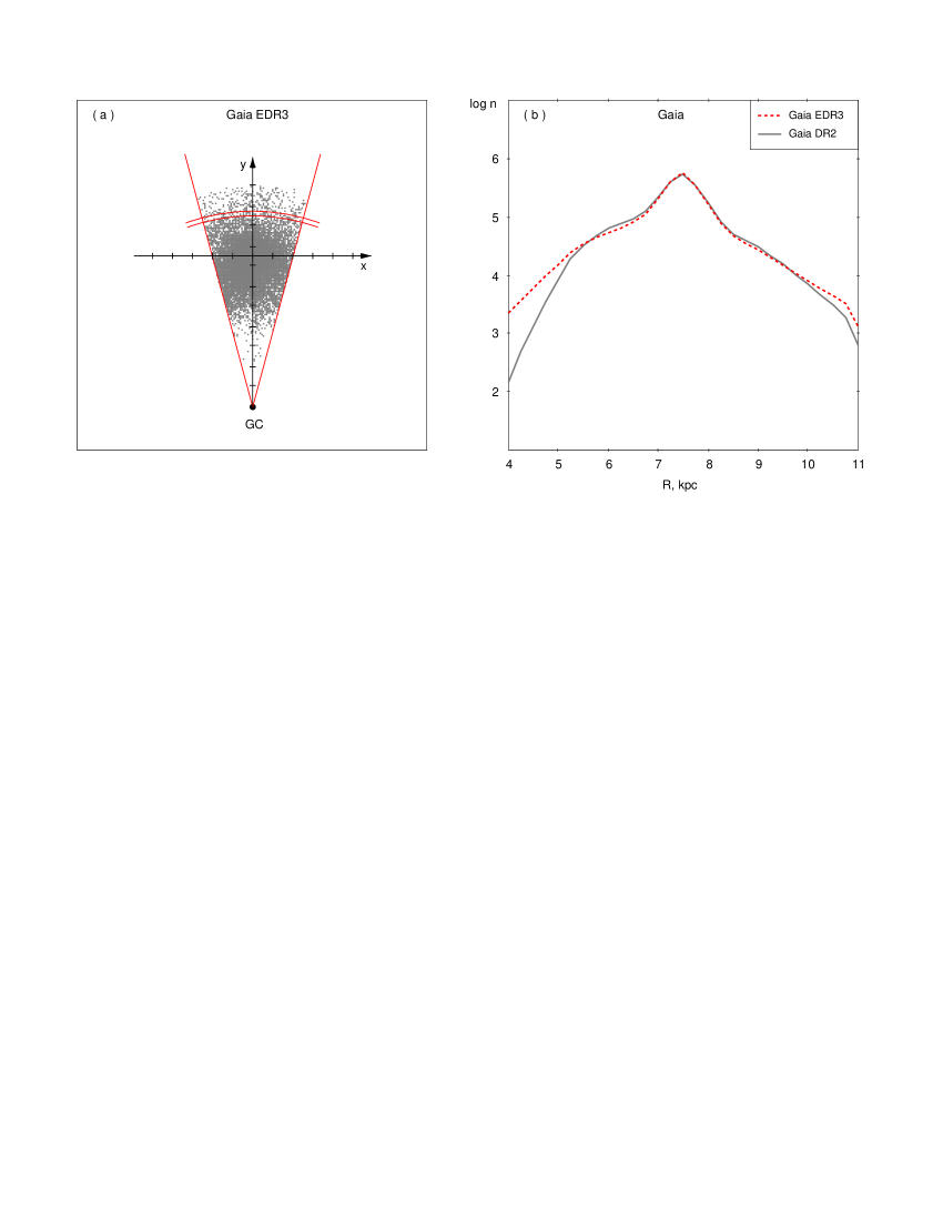
Figure 1: (a) Distribution of Gaia EDR3 stars located near the Galactic plane, $|z|<200$ pc, and in the sector of the Galactocentric angles $|\theta|<15^{\circ}$ (gray points). We selected Gaia EDR3 stars with reliable parallaxes, known proper motions and line-of-sight velocities. Only 1 per cent of objects are shown. For an example, we outlined one $\Delta R=250$-pc wide bin by two arcs. The Galactic center (GC) is at the bottom, the axes $x$ and $y$ are directed toward the Galactic rotation and away from the Galactic center, respectively; the Sun is at the origin. (b) Logarithmic dependencies of the numbers of stars, $n$, in 250-pc wide bins on the distance $R$ derived from the Gaia EDR3 and Gaia DR2 data.

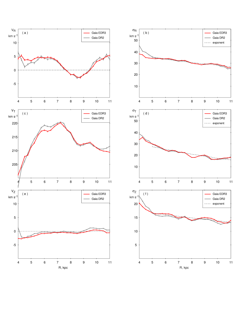
Figure 2: Variations in the velocity components, $V_{R}$, $V_{T}$ and $V_{Z}$ (left panel), and in the velocity dispersions, $\sigma_{R}$, $\sigma_{T}$ and $\sigma_{Z}$ (right panel), along the Galactocentric distance, $R$, derived from the Gaia EDR3 and Gaia DR2 data. The median velocities are calculated in 250-pc wide bins. The vertical lines on the curves demonstrate the random errors in the determination of the velocities and velocity dispersions. We can see (a) that the radial velocity $V_{R}$ reaches a maximum of +5 km s^-1 at the distance of $R\sim 6$ kpc and a minimum of $V_{R}\sim-3$ km s^-1 at $R\sim 8.5$ kpc. Note also that the $V_{R}$-profile derived from the Gaia DR3 data is flatter in the distance interval 4–6 kpc than the profile derived from the Gaia DR2 catalogue. (c) The profile of the azimuthal velocity $V_{T}$ demonstrates a sharp drop by $\Delta V_{T}=7$ km s^-1 in the distance interval $R=7.0$–8.5 kpc. Noticeably lower velocities $V_{T}$ in the distance range 4.0–5.5 kpc can be due to the lack of thin-disc stars in this region. (e) The vertical velocity $V_{Z}$ remains within $\pm 1$ km s^-1 in the distance interval 6.0–9.0 kpc but exhibits a velocity bend at the larger distances from the Sun, which can be due to the wrong distance scale. (b, d, f) The variations in the velocity dispersions, $\sigma_{R}$, $\sigma_{T}$ and $\sigma_{Z}$, with the distance $R$ were approximated by the exponential law (the dashed lines).

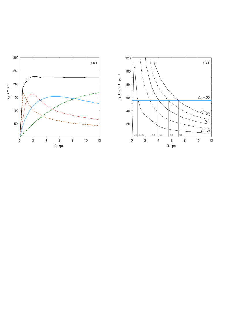
Figure 3: (a) Model rotation curve. The total rotation curve (the black curve) and the contribution of the bulge, bar, disc and halo (the brown, red, blue and green curves, respectively) to the rotation curve. (b) Dependencies of the angular velocities $\Omega$, $\Omega\pm\kappa/2$ (the solid curves) and $\Omega\pm\kappa/4$ (the dashed curves) on the distance $R$. The horizontal straight line (coloured in blue) indicates the angular velocity of the bar and its intersections with the curves of angular velocities mark the locations of the resonances.

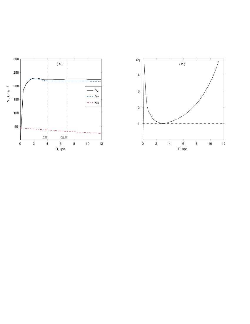
Figure 4: Initial velocity distribution of model particles. (a) Velocities of the rotation curve $V_{c}$ (solid line), the average azimuthal velocities $\overline{V_{T}}$ (dashed line) and the initial velocity dispersion $\sigma_{R}$ (dash-and-dot line) of model particles. (b) Dependence of the Toomre disc stability parameter $Q_{T}$ on Galactocentric distance $R$ built for the initial velocity distribution.

3 Model

3.1 General remarks

In the previous section we showed that there are no conspicuous systematic motions in the direction perpendicular to the Galactic disc in the vicinity of $|R-R_{0}|<1.5$ kpc from the Sun. So the motions in the Galactic plane and in the vertical direction can be thought to be independent, which gives us a possibility to consider a 2D model of the Galaxy.

We built a model of the Galaxy that includes the bulge, bar, exponential disc and halo. The bar is modelled as a Ferrers ellipsoid with the volume-density distribution $\rho$ defined as follows:

$$\rho=\left\{\begin{array}[]{l}\rho_{0}(1-\xi^{2})^{n},\ \xi\leq 1\\ \\ 0,\ \xi>1,\\ \end{array}\right.$$ (12)

where $\rho_{0}$ is the central density, $\xi$ equals $\xi^{2}=x^{2}/a^{2}+y^{2}/b^{2}$ but $a$ and $b$ are the lengths of the major and minor semi-axes of the bar, respectively. The exponent $n$ is adopted to be $n=2$. The mass of the bar $M_{b}$ and the central density $\rho_{0}$ are related by the expression:

$$M_{b}=\rho_{0}\,\frac{32\pi ab^{2}}{105}$$ (13)

(Freeman, 1970; Athanassoula et al., 1983; Pfenniger, 1984; Binney & Tremaine, 2008; Sellwood & Wilkinson, 1993).

The main model requirement is that the model must reproduce the observed profiles of the radial, $V_{R}$, and azimuthal, $V_{T}$, velocities as well as the profiles of the velocity dispersions, $\sigma_{R}$ and $\sigma_{T}$ (Fig. 2). In addition, the model rotation curve must be flat on the Galactic periphery and have the angular velocity of $\Omega_{0}=30$ km s^-1 kpc^-1 at the solar distance, which agrees with observations and corresponds to the solar azimuthal velocity $V_{T0}=\Omega_{0}R_{0}+12$ km s^-1 used for calculations of stellar velocities with respect to the Galactic center (section  2).

We adopted the simulation time to be $T=3$ Gyr. The model includes $N=10^{7}$ particles that simulate the motion of stars in the Galactic disc. This number is enough to produce the velocity profiles with an accuracy comparable to the observational one.

Fig. 3(a) shows the contribution of the bulge, bar, disc and halo to the total rotation curve. The total rotation curve is practically flat on the periphery and corresponds to the angular velocity of the disc rotation at the solar distance equal to $\Omega_{0}=30.0$ km s^-1 kpc^-1.

Fig. 3(b) shows the dependencies of the angular velocities $\Omega$, $\Omega\pm\kappa/2$ and $\Omega\pm\kappa/4$ on Galactocentric distance $R$. The horizontal line indicates the angular velocity of the bar, and its intersections with the curves of angular velocities mark the locations of the resonances.

Table 2 lists the model parameters of the bar, bulge, disc and halo. The semi-major and semi-minor axes of the bar are adopted to be $a=3.5$ and $b=1.35$ kpc, respectively. The mass of the bar is 1.2 10¹⁰ M_⊙. The angular velocity of the bar is taken to be $\Omega_{b}=55$ km s^-1 kpc^-1, which corresponds to the location of the corotation radius $(\Omega=\Omega_{b})$ and the OLR of the bar at the distances of $R_{CR}=4.04$ kpc and $R_{OLR}=7.00$ kpc, respectively. The model also includes two Inner Lindblad Resonances (ILRs) located at the distances of $R_{ILRI}=0.14$ and $R_{ILRO}=0.87$ kpc.

Non-axisymmetric perturbations of the bar increase slowly approaching the full strength by $T_{gr}=447$ Myr, which is equal to four bar rotation periods. However, the $m=0$ component of the bar is included in the model from the beginning. During the period of the bar growth, $0<t<T_{gr}$, radial and azimuthal forces created by the bar were multiplied by the factor $k_{g}$ which increases linearly from 0 to 1. We also introduce the additional force, $f_{a}$, which on the contrary decreases linearly with time:

$$\left\{\begin{array}[]{lc}k_{g}=t/T_{gr}&\\ &0<t<T_{gr},\\ f_{a}=(1-k_{g})\,<f_{b}>&\\ \end{array}\right.\\$$ (14)

where $<f_{b}>$ is the radial force created by the bar averaged over the azimuthal angle $\theta\in[0,2\pi]$. The force $<f_{b}>$ depends on the radius, $R$, so its values were tabulated before the simulation and then were calculated for a position of a particle by linear interpolation. This procedure ensures a constant average radial force at each radius during the bar-growth period. The $m=0$ component of the bar can be interpreted as a pre-existent disc-like bulge (Athanassoula, 2005).

The $q_{t}(R)$ quantity is often considered as the characteristic of perturbations created by a bar. It is calculated as the maximal ratio of the acceleration in the azimuthal direction to the average acceleration in the radial direction at a certain radius:

$$q_{t}(R)=\textrm{max}(\frac{\max(|F_{T}|)}{<|F_{R}|>}).$$ (15)

The strength of the bar, $Q_{b}$, is determined as the maximal value of $q_{t}$ along the radius (Sanders & Tubbs, 1980; Combes & Sanders, 1981; Athanassoula et al., 1983). In the present model the strength of the bar amounts to $Q_{b}=0.3142$, which is a typical value for galaxies with strong bars (Block et al., 2001; Buta, Laurikainen & Salo, 2004; Díaz-García et al., 2016).

The model of the Galaxy includes an exponential disc with a mass of $M_{d}=3.25$ 10¹⁰M_⊙ and a characteristic scale of $R_{d}=2.5$ kpc (Bland-Hawthorn & Gerhard, 2016). The total mass of the model disc and bar is $M_{d}+M_{b}=4.45\times 10^{10}$M_⊙, which agrees with other estimates of the Galactic-disc mass lying in the range 3.5–5.0$\times 10^{10}$M_⊙ (Shen et al., 2010; Fujii et al., 2019). The surface density of the disc is determined by the relation:

$$\Sigma=\Sigma_{0}\,\exp^{-\frac{R}{R_{D}}},$$ (16)

where $\Sigma_{0}$ is the density of the disc at the Galactic center. Here we consider only the thin disc because the ratio of the surface densities of the thick and thin discs are supposed to be only 12 per cent at the solar distance (as a review Bland-Hawthorn & Gerhard, 2016).

The classical bulge is modelled by a Plummer sphere with the mass of $M_{bg}=5\times 10^{9}$ (Dehnen & Binney, 1998; Nataf, 2017; Fujii et al., 2019). The halo is modelled by an isothermal sphere. More detailed description of the construction method for each Galactic subsystem is given in Melnik (2019).

Table 2: Model parameters

Simulation time	$T=3$ Gyr
Step of integration	$\Delta t=0.01$ Myr
Number of particles	$N=10^{7}$
Bulge	$R_{bg}=0.30$ kpc
	$M_{bg}=5$ 109M⊙
Bar	$a=3.5$ and $b=1.35$ kpc
	$M_{b}=1.20$ 1010M⊙
	$\Omega_{b}=55.0$ km s-1 kpc-1
	$T_{gr}=447$ Myr
Disc	exponential, $R_{d}=2.5$ kpc
	$M_{d}=3.25$ 1010M⊙
Halo	$R_{h}=8$ kpc
	$V_{max}=201.4$ km s-1

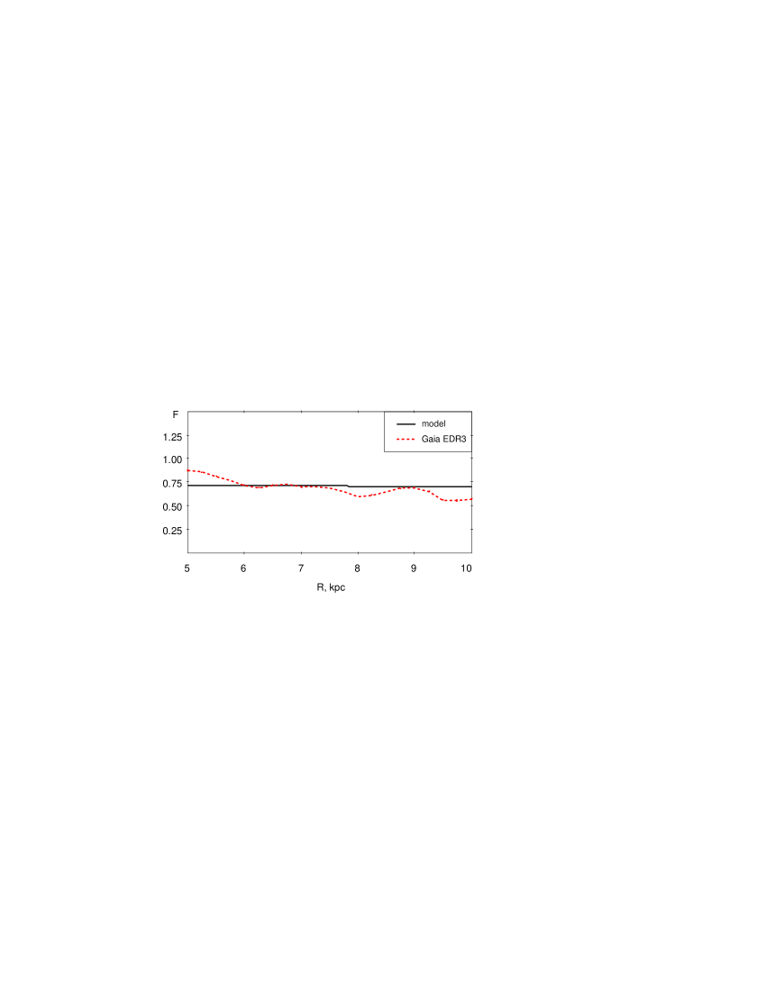
Figure 5: Dependence of the ratio of the observed velocity dispersions, $\sigma_{T}/\sigma_{R}$, derived from the Gaia EDR3 data (the red dashed line) and the model value $F=\kappa/(2\Omega)$ (the black line) on Galactocentric distance $R$. The value of $F$ determines the ratio of the azimuthal and radial velocity dispersions adopted for the initial distribution of model particles.

3.2 The initial velocity distribution

We suppose that 3 Gyr ago the dependence of the radial velocity dispersion $\sigma_{R}$ on the distance $R$ in the $R=5$–11 kpc interval was similar to what is observed now:

$$\sigma_{R}=C^{*}_{R}\exp^{-\frac{R}{S_{R}}},$$ (17)

where $S_{R}$ is adopted to be $S_{R}=20$ kpc (Eq. 9).

We want to make sure that the model disc is stable against axisymmetric perturbations at the initial time instant. So the value of the constant $C^{*}_{R}$ is determined so as to ensure the Toomre stability parameter would be $Q_{T}\geq 1$ throughout the disc (Toomre, 1964). In our model, $Q_{T}$ achieves a minimum at the distance of $R=3.1$ kpc, so the constant $C^{*}_{R}$ is determined from the equation:

$$Q_{T}=\frac{\sigma_{R}\,\kappa}{3.36\,G\,\Sigma}=1$$ (18)

at the distance of $R=3.1$ kpc (Fig. 4b). This normalization yields the initial radial-velocity dispersion at the solar distance of $\sigma_{R}=30.5$ km s^-1, which is very close to the value of $\sigma_{R}=31.5$ km s^-1 derived from the smooth distribution of the Gaia velocity dispersions (Eq. 9). After the model bar started growing, the velocity dispersion inside the corotation radius ($R_{CR}=4.0$ kpc) increased rapidly but we want the disc to be stable at the initial moment as well (see also section  4.5).

Any subsystem of disc stars with a non-zero velocity dispersion rotates with a smaller average velocity than the velocity of the rotation curve (for example, Binney & Tremaine, 2008). The relation between the average azimuthal velocity $\overline{V_{T}}$ and the velocity of the rotation curve $V_{c}$ is determined by the Jeans equation:

$$\frac{\partial(\rho\overline{V^{2}_{R}})}{\partial R}+\frac{\partial(\rho\overline{V_{R}V_{z}})}{\partial z}+\rho\;(\frac{\overline{V^{2}_{R}}-\overline{V^{2}_{T}}}{R}+\frac{\partial\Phi}{\partial R})=0,$$ (19)

where $\rho$ is the volume density of disc stars and $\Phi$ is the Galactic potential which is related to the velocity of the rotation curve by the following expression:

$$V^{2}_{c}=R\,\frac{\partial\Phi}{\partial R}.$$ (20)

Assuming that the motions along coordinates $R$ and $z$ are independent, we can neglect the second term in the left part of Eq. 19. If we suppose that the distribution law along the coordinate $z$ does not depend on the distance $R$, then we can substitute the volume density $\rho$ for the surface density $\Sigma$. We assume that systematic motions are absent at the initial moment and can make following substitutions:

$$\overline{V^{2}_{R}}=\sigma^{2}_{R},$$ (21)

$$\overline{V^{2}_{T}}=\overline{V_{T}}^{2}+\sigma^{2}_{T},$$ (22)

which allows us to rewrite the Jeans equation in the following way:

$$\overline{V_{T}}^{2}=V^{2}_{c}+\sigma_{R}^{2}-\sigma_{T}^{2}+\frac{R}{\Sigma}\frac{\partial(\Sigma\sigma_{R}^{2})}{\partial R}.$$ (23)

Assuming the epicyclic approximation for the initial velocity distribution, we can write the following relation between the velocity dispersions along the radial and azimuthal directions:

$$\frac{\sigma_{T}}{\sigma_{R}}=\frac{\kappa}{2\,\Omega}.$$ (24)

We now use Eqs. 9, 16 and 24 to obtain:

$$\overline{V_{T}}^{2}=V_{c}^{2}+\sigma_{R}^{2}(1-\frac{\kappa^{2}}{4\Omega^{2}}-\frac{R}{R_{D}}-\frac{2R}{S_{R}}),$$ (25)

where $\overline{V_{T}}$ is the average azimuthal velocity of model particles at the initial time instant.

Fig. 4(a) shows the distribution of the average azimuthal velocity, $\overline{V_{T}}$, of model particles along Galactocentric distance, $R$, at the initial instant. Also shown are the velocity of the rotation curve, $V_{c}$, and the radial-velocity dispersion, $\sigma_{R}$, at the initial moment. We can see that the velocity $\overline{V_{T}}$ is always slightly lower than the velocity of the rotation curve and the difference $V_{c}-\overline{V_{T}}$ increases with the increasing distance $R$.

Fig. 5 shows the dependence of the ratio of the observed velocity dispersions of disc stars, $\sigma_{T}/\sigma_{R}$, and the model value $F=\kappa/(2\Omega)$ on Galactocentric distance $R$. The value of $F$ determines the ratio of the azimuthal and radial velocity dispersions adopted for the initial distribution of model particles. We can see that $F$ is almost constant and varies in the range $F=0.70$–0.72 in the distance interval 5–10 kpc, which is quite expected for model with a flat rotation curve for which $F$ must be equal to $F=1/\sqrt{2}$. The formal errors in the determination of the observed ratio $\sigma_{T}/\sigma_{R}$ are less than 0.01. The model value $F=\kappa/(2\Omega)$ is derived from the model potential so it is absolutely accurate. We can see that the Gaia EDR3 ratio of the velocity dispersions, $\sigma_{T}/\sigma_{R}$, decreases with increasing distance $R$, which can be due to the rapid change of the velocity dispersion $\sigma_{T}$ with $R$ (Table 1). However, in the solar neighborhood of $|R-R_{0}|<1.5$ kpc, the observed ratio $\sigma_{T}/\sigma_{R}$ lies in the range 0.60–0.72. So here the model and observed values of the velocity dispersions are consistent to within 15%.

4 Results

4.1 Formation of the rings

The formation of elliptical resonance rings requires some time for the epicyclic motions of stars to adjust in accordance with the rotation of the bar. Fig. 6 shows the distribution of the surface density of model particles in the Galactic disc at different time instants. The time $t=0$ corresponds to the instant when the bar is turned on. By the time $T_{gr}=0.45$ Gyr the bar gains the full strength. One can see that the outer rings, $R_{1}$ and $R_{2}$, are already formed by the time $t=1$ Gyr. The ring $R_{1}$ is located closer to the Galactic center and is stretched perpendicular to the bar so that the bar and ring $R_{1}$ are reminiscent of the Greek letter ’$\theta$’. The ring $R_{2}$ is located further away from the Galactic center and is stretched parallel to the bar. Besides the outer rings, $R_{1}$ and $R_{2}$, the Galactic disc produces the inner ($r$) and nuclear ($n$) resonance rings.

Fig. 7(a) shows the distribution of the surface density, $\Sigma$, of model particles along the distance $R$ at different time moments. Local density minima between the following pairs of rings: $n$ and $r$, $r$ and $R_{1}$, $R_{1}$ and $R_{2}$, are immediately apparent. Interestingly, the location on the OLR precisely coincides with the density minimum.

Fig. 7(b) shows the distribution of the relative surface density, $\Delta\Sigma=\Sigma-\Sigma_{0}+C$, of model particles near the OLR. The function $\Sigma_{0}$ describes the exponential density distribution at the start of the simulation but the constant $C=3.2$ 10³ kpc^-2 is added to avoid dealing with negative values. We can see some variations in the width and density of the outer ring $R_{2}$: at the times $t=2.0$ and 3.0 Gyr the ring $R_{2}$ has larger width and smaller density than at the times $t=1.5$ and 1.0 Gyr, which is mainly due to the shift of its inner boundary. Probably, here we see the periodically strengthening and weakening ring $R_{2}$.

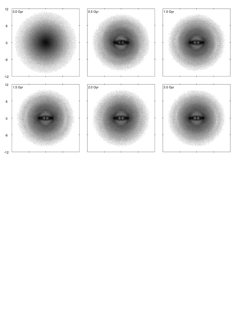
Figure 6: Distribution of the surface density of model particles in the Galactic disc at different time moments. The size of the frames is $24\times 24$ kpc. The major axis of the bar is oriented horizontally. Two closest shades of gray correspond to a density change by a factor of 0.8. The model galaxy rotates counterclockwise.

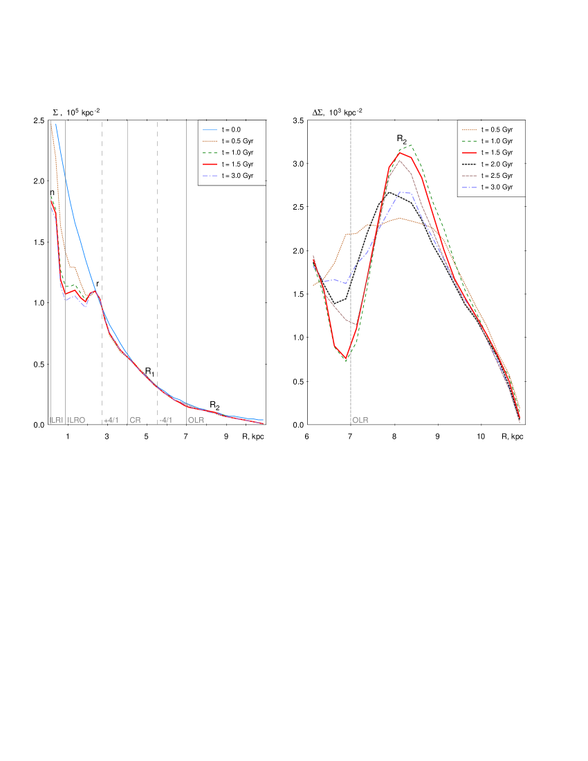
Figure 7: (a) Distribution of the surface density, $\Sigma$, of model particles along Galactocentric distance $R$ at different time instants. The locations of the resonance rings are marked by the letters: $n$ (nuclear ring), $r$ (inner ring), $R_{1}$ and $R_{2}$ (outer rings). (b) Distribution of the relative surface density, $\Delta\Sigma=\Sigma-\Sigma_{0}+C$, of model particles near the OLR, where $\Sigma_{0}$ is the initial exponential density distribution but the constant $C=3.2$ 10³ kpc^-2 is added to avoid dealing with negative values. We can see some variations in the width and density of the outer ring $R_{2}$: the ring $R_{2}$ has a flatter profile at the times $t=2.0$ and 3.0 Gyr than at the times $t=1.0$ and 1.5 Gyr.

4.2 Comparison between the model and observed velocity profiles

Fig. 8 shows the model and observed dependencies of the radial, $V_{R}$, and azimuthal, $V_{T}$, velocities of disc stars lying in the sector $|\theta|<15^{\circ}$ on Galactocentric distance $R$. The model dependencies are obtained for the angular velocity and the position angle of the bar equal to $\Omega_{b}=55$ km s^-1 kpc^-1 and $\theta_{b}=45^{\circ}$, respectively. The position angle of the bar close to $\theta_{b}=45^{\circ}$ is found in many studies (Hammersley et al., 2000; Benjamin et al., 2005; Cabrera-Lavers et al., 2007; Melnik & Rautiainen, 2009; González-Fernández et al., 2012; Pettitt et al., 2014, and other papers). The median velocities of model particles were calculated in $\Delta R=250$-pc wide bins. Model velocity profiles were averaged over 0.5 Gyr time periods with a step of $\Delta t=0.01$ Gyr. The random errors in the determination of the average model velocities in bins are smaller than 0.1 km s^-1. The observed velocity profiles were derived from the Gaia EDR3 data (section 2).

Fig. 8 (left panel) shows the model and observed profiles of the radial velocity $V_{R}$. The model $V_{R}$-profiles demonstrate a plateau in the distance interval $R=5.0$–6.0 kpc, a smooth fall from the velocity $V_{R}=+5$ to $-3$ km s^-1 over the interval $R=6.0$–8.5 kpc and a slow rise or a plateau with a constant negative velocity $V_{R}$ in the interval $R=8.5$–10.0 kpc. We can see that the model and observed $V_{R}$-profiles match well in the distance interval $R=6$–9 kpc. Note that the model profiles of the velocity $V_{R}$ obtained during the time periods $t=0.5$–1.0 and 1.0–1.5 Gyr are steeper than the profiles calculated for the periods 1.5–2.0, 2.0–2.5 and 2.5–3.0 Gyr, which can result from a small increase in the velocity dispersion due to the tuning of the epicyclic motions near the OLR (i.e. to the formation of the outer rings). Generally, the model and observed $V_{R}$-profiles match better during the time periods 1.5–2.0, 2.0–2.5 and 2.5–3.0 Gyr than at the times 0.5–1.0 and 1.0–1.5 Gyr.

Fig. 8 (right panel) shows the model and observed profiles of the azimuthal velocity $V_{T}$. The model velocity $V_{T}$ is almost constant, $V_{T}=216$–218 km s^-1, at the start of the simulation (the slightly curved dashed line). The velocity $V_{T}$ drops by 5 km s^-1 at the distance of $R=8.5$ kpc by the time $t=1.0$ Gyr. We can see that the model and observed $V_{T}$-profiles agree well over the distance interval $R=6.0$–10.0 kpc at the time periods 1.0–1.5 and 1.5–2.0 Gyr. The model can reproduce the sharp drop of the velocities $V_{T}$ in the distance interval $R=7.5$–8.5 kpc just at the times 1.0–1.5 and 1.5–2.0 Gyr, but later the model velocity $V_{T}$ demonstrates a smoother fall.

The study of the influence of the observational errors and selection effects onto the distributions of the velocities $V_{R}$ and $V_{T}$ along the distance $R$ is presented in Appendix.

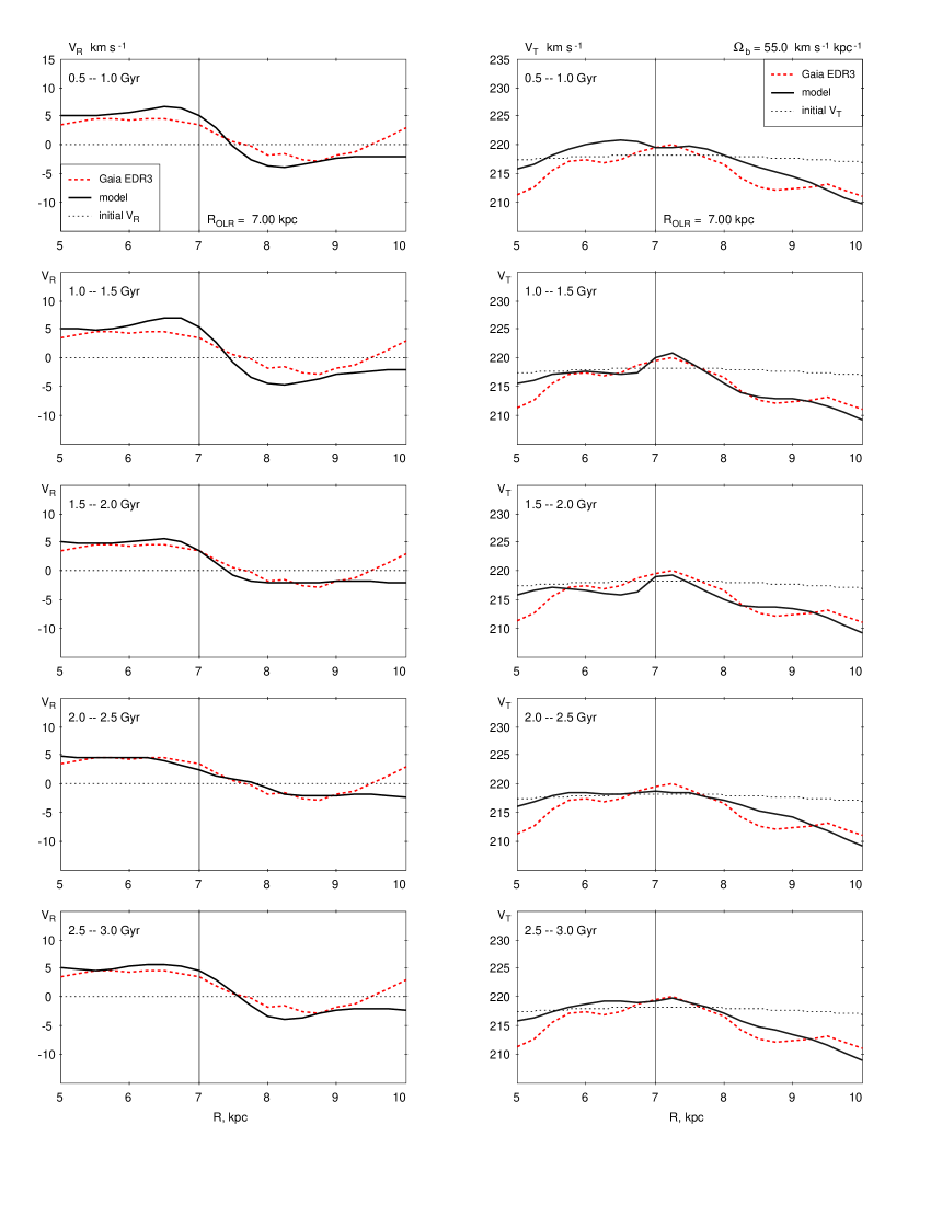
Figure 8: Model and observed dependencies of the median radial and azimuthal velocities, $V_{R}$ and $V_{T}$, of disc stars lying in the sector $|\theta|<15^{\circ}$ on Galactocentic distance $R$. The model velocity profiles (the black curves) are obtained for the angular velocity and the position angle of the bar equal to $\Omega_{b}=55$ km s^-1 kpc^-1 and $\theta_{b}=45^{\circ}$, respectively, and averaged over the time periods of 0.5 Gyr. The observed velocity profiles (the red dashed curves) are derived from the Gaia EDR3 data. The errors in determination of both Gaia EDR3 and model average velocities in bins are smaller than the line width. The dashed gray lines indicate the initial distribution of the velocities $V_{R}$ and $V_{T}$. The boundaries of time periods are shown at each frame. The vertical lines indicate the location of the OLR.

4.3 Comparison of the velocity profiles during different time periods

We calculated the statistics $\chi^{2}$ (the sum of squared differences between the model and observed velocities) to find the time periods during which the model and observed velocity profiles agree best. The values of $\chi^{2}_{R}$ and $\chi^{2}_{T}$ are computed in $n=17$ bins in the distance interval $R=5.5$–9.5 kpc for the radial and azimuthal velocity profiles, respectively:

$$\chi^{2}_{R}=\sum^{n}\frac{(V_{R,\,\textrm{mod}}-V_{R,\,\textrm{obs}})^{2}}{\varepsilon_{VR}^{2}},$$ (26)

$$\chi^{2}_{T}=\sum^{n}\frac{(V_{T,\,\textrm{mod}}-V_{T,\,\textrm{obs}})^{2}}{\varepsilon_{VT}^{2}},$$ (27)

where $\varepsilon_{VR}$ and $\varepsilon_{VR}$ are the average uncertainties in the determination of the model and observed velocities $V_{R}$ and $V_{T}$ in bins. The uncertainties in the determination of observational velocities $V_{R}$ and instantaneous model velocities $V_{R}$ (obtained without averaging over the time) are 0.2 and 0.3 km s^-1, so we adopted $\varepsilon_{VR}=0.5$ km s^-1. The uncertainties $\varepsilon_{VR}$ and $\varepsilon_{VT}$ are connected through the relation:

$$\varepsilon_{VT}=\frac{\kappa}{2\,\Omega}\;\,\varepsilon_{VR},$$ (28)

where the coefficient $\kappa/(2\Omega)$ equals 0.71 in the interval $R=5.5$–9.5 kpc (Fig. 5, black line).

Fig. 9 shows the variations in the values of $\chi^{2}_{R}$ and $\chi^{2}_{T}$ as well as in their sum $\chi^{2}=\chi^{2}_{R}+\chi^{2}_{T}$ with time $t$. A step in time is $\Delta t=10$ Myr. We can see that the $\chi^{2}_{R}$, $\chi^{2}_{T}$ and $\chi^{2}$ functions demonstrate small oscillations about the average values, which are due to the stochastic deviations of the velocities of model particles. The $\chi^{2}$ function starts its decrease at $t=0.5$ Gyr and reaches a plateau at the time 1 Gyr. The distribution of $\chi^{2}$ in the time period 1–3 Gyr is not precisely flat but exhibits a shallow minimum at $t=1.8$ Gyr. The location of the minimum is determined with the uncertainty of $\pm 0.5$ Gyr corresponding to $1\sigma$ probability level.

It is just observational data derived from the Gaia EDR3 catalogue that produce the minimum at $t=1.8\pm 0.5$ Gyr. A comparison of our model with the velocity profiles derived from the Gaia DR2 catalogue does not yield a minimum at the time period 1–3 Gyr.

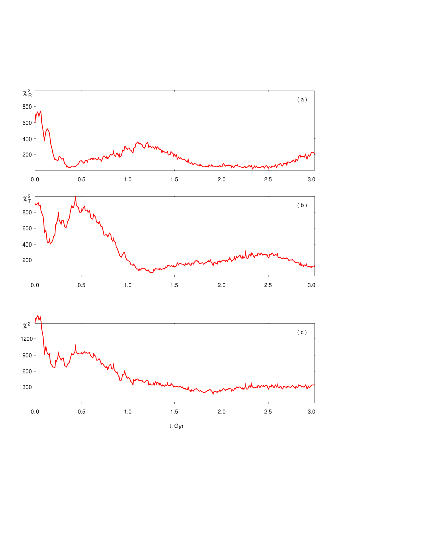
Figure 9: The functions $\chi^{2}_{R}$, $\chi^{2}_{T}$ and their sum $\chi^{2}=\chi^{2}_{R}+\chi^{2}_{T}$. The $\chi^{2}$ function reaches a minimum at the time $1.8\pm 0.5$ Gyr.

4.4 Comparison of the velocity profiles calculated for different values of $\Omega_{b}$ and $\theta_{b}$

Fig. 10 shows the distributions of the radial and azimuthal velocities, $V_{R}$ and $V_{T}$, along Galactocentric distance $R$ calculated for five values of the bar angular velocity: $\Omega_{b}=40$, 45, 55 and 60 km s^-1 kpc^-1. The position angle of the bar is supposed to be $\theta_{b}=45^{\circ}$. Model velocity-profiles are averaged for the time period of $t=1.5$–2.0 Gyr. We can see that the value of the bar angular velocity equal to $\Omega_{b}=55$ km s^-1 kpc^-1 provides the best agreement between the model and observed $V_{R}$- and $V_{T}$-velocity profiles. Note, that the model velocity profiles computed, on the one hand, for the speeds of $\Omega_{b}=40$, 45, 50 km s^-1 kpc^-1 and, on the other hand, for 60 km s^-1 kpc^-1 are shifted with respect to the observed profiles towards larger and smaller distances $R$, respectively. The larger the bar angular velocity $\Omega_{b}$, the smaller the radius of the OLR. Fig. 10 also shows that the radial velocity $V_{R}$ starts decreasing nearly at the radius of the OLR while the azimuthal velocity $V_{T}$ demonstrates a slight rise just at the distance of the OLR and starts its drop only at the distance exceeding the radius of the OLR by nearly 0.7 kpc: $R\sim R_{OLR}+0.7$ kpc.

Fig. 11(a) shows variations in the $\chi^{2}$ values averaged over the time periods $t=1.0$–1.5, 1.5–2.0, and 2.5–3.0 Gyr as a function of the bar angular velocity $\Omega_{b}$. The vertical lines indicate the dispersions of the $\chi^{2}$ values. We can see that the $\chi^{2}$ functions achieve minima at $\Omega_{b}=55$ km s^-1 kpc^-1. The 1$\sigma$ confidence interval calculated for the time period 1.5–2.0 Gyr is 52–57 km s^-1 kpc^-1. The function $\chi^{2}$ computed for the time period 1.5–2.0 Gyr achieves smaller values than $\chi^{2}$ obtained for other periods but the difference is close to 1$\sigma$.

The value of the bar angular velocity of $\Omega_{b}=55$ km s^-1 kpc^-1 corresponds to the location of the OLR of the bar at $R_{OLR}=7.00$ kpc. The adopted value of the solar Galactocentric distance is $R_{0}=7.5$ kpc, so the radius of the OLR must be shifted by 0.5 kpc towards the Galactic center with respect to the solar circle. The uncertainty in the values of $\Omega_{b}$, 52–57 km s^-1 kpc^-1, produces the uncertainty in the radius of the OLR equal to 6.75–7.40 kpc and the shift of the OLR with respect to the solar circle is determined with the uncertainty $R_{OLR}=R_{0}-0.5_{-0.3}^{+0.4}$ kpc.

The position angle of the bar, $\theta_{b}$, is the angle between the direction of the bar major axis and the Sun–Galactic center line. Fig. 11(b) shows variations in the $\chi^{2}$ values averaged over the time periods $t=1.0$–1.5, 1.5–2.0, and 2.5–3.0 Gyr with the position angle $\theta_{b}$. We can see that the $\chi^{2}$ function built for the time period 1.5–2.0 Gyr demonstrates a sharp drop at the interval 0–30^∘ followed by a plateau with a shallow minimum at $\sim 45^{\circ}$. The 1$\sigma$ confidence interval for the location of the minimum is $\theta_{b}=25$–$60^{\circ}$.

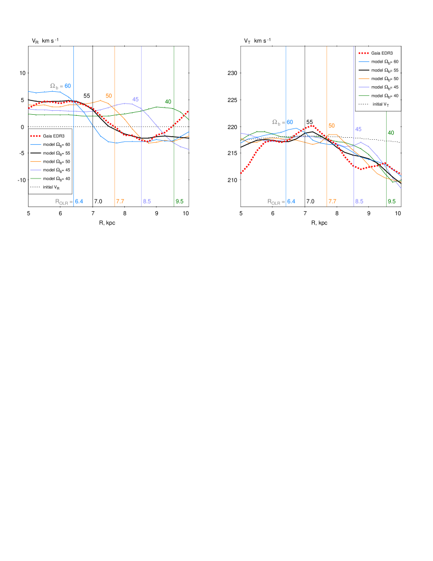
Figure 10: Model and observed distributions of the radial $V_{R}$ (left panel) and azimuthal $V_{T}$ (right panel) velocities along Galactocentric distance $R$. The model velocity profiles are calculated for the five values of the bar angular velocity: $\Omega_{b}=40$ (green line), 45 (violet line), 50 (yellow line), 55 (thick black line) and 60 (blue line) km s^-1 kpc^-1, and are averaged over the time period of $t=1.5$–2.0 Gyr. The observed velocity profiles are derived from the Gaia EDR3 data (red dashed curves). The long vertical lines indicate the locations of the OLRs. The upper row of colored numbers displays the values of $\Omega_{b}$ while the bottom row gives the values of $R_{OLR}$. The strokes on the curves indicate the random errors in the determination of the model median velocities in bins averaged over 50 profiles. The errors in the determination of the observed velocities in bins are comparable with the line width. We can see that the bar angular velocity of $\Omega_{b}=55$ km s^-1 kpc^-1 provides the best agreement between the model and observed velocity profiles while the values of $\Omega_{b}=40$–50 and 60 km s^-1 kpc^-1 cause the model velocity profiles to be shifted towards larger and smaller distances $R$, respectively.

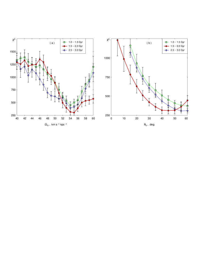
Figure 11: Variations in the $\chi^{2}$ values averaged over the time periods $t=1.0$–1.5, 1.5–2.0 and 2.5–3.0 Gyr (a) along the angular velocity of the bar, $\Omega_{b}$, and (b) along the position angle of the bar, $\theta_{b}$. The vertical lines indicate the dispersions of the $\chi^{2}$ values. The $\chi^{2}$ function calculated for the time period 1.5–2.0 Gyr achieves smaller values than $\chi^{2}$ obtained for other time periods but the difference is close to 1$\sigma$. (a) The minima of the $\chi^{2}$ functions correspond to the value of $\Omega_{b}=55$ km s^-1 kpc^-1. The 1$\sigma$ confidence interval calculated for the time period 1.5–2.0 Gyr is $\Omega_{b}=52$–57 km s^-1 kpc^-1. (b) The $\chi^{2}$ function built for the time period 1.5–2.0 Gyr demonstrates a sharp drop at the interval 0–30^∘ followed by a plateau with a shallow minimum at $\sim 45^{\circ}$. The 1$\sigma$ confidence interval for the location of the minimum is $\theta_{b}=25$–$60^{\circ}$.

4.5 Comparison between the model and observed velocity dispersions

Figure 12 shows variations in the dispersions of the radial, $\sigma_{R}$, and azimuthal, $\sigma_{T}$, velocities with the distance $R$ calculated for the model and observed velocities. The model $\sigma_{R}$- and $\sigma_{T}$-profiles are plotted with the time step of $\Delta t=0.2$ Gyr. We can see that the model velocity dispersions, $\sigma_{R}$ and $\sigma_{T}$, demonstrate a fast growth inside the corotation radius $R<4.0$ kpc during the first 0.6 Gyr, after which changes become very small. But beyond this radius, $R>4.0$ kpc, the velocity dispersions change only slightly during the entire simulation time. However, we can notice a small growth of the radial velocity dispersion, $\sigma_{R}$, near the OLR: from the initial value of $\sigma_{R}=31.6$ km s^-1 ($t=0$) to maximum of 34.7 km s^-1 at $t=1.3$ Gyr and then back to 32.8 km s^-1 at $t=2.5$ Gyr. Probably, such small up-and-down changes are due to the tuning of orbits near the resonance rings $R_{1}$ and $R_{2}$ (see discussion in Melnik, 2019). Generally, the model and observed velocity dispersions agree to within $\sim 15$ per cent in the distance interval $R=6$–9 kpc.

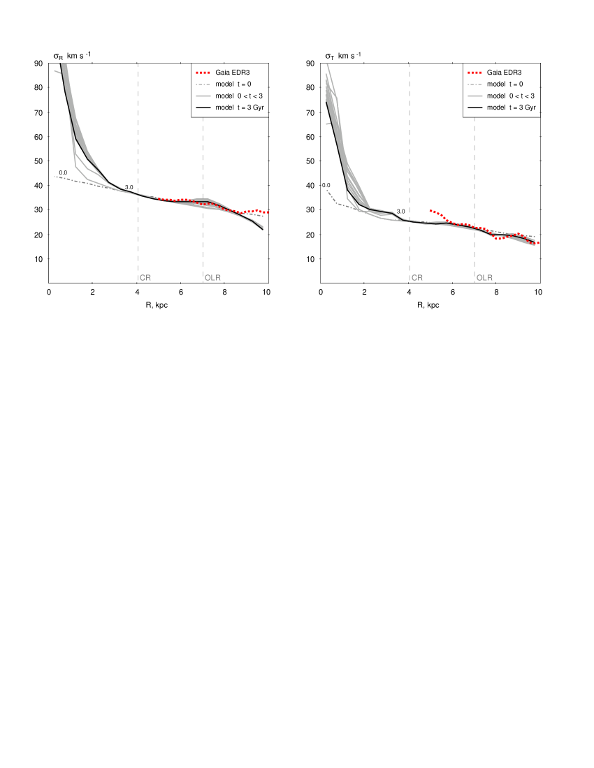
Figure 12: Variations in the radial, $\sigma_{R}$, and azimuthal, $\sigma_{T}$, velocity dispersions as a function of Galactocentric distance $R$ obtained for the model (black and gray curves) and observed (red dashed curves) velocities. The model profiles of the velocity dispersions are plotted with the time step of $\Delta t=0.2$ Gyr. The model velocity dispersions demonstrate a fast increase inside the corotation radius $R<4.0$ kpc during the first 0.6 Gyr after which changes are very small. But beyond this radius, $R>4.0$ kpc, the velocity dispersions change only slightly during the entire simulation time. However, we can notice a small growth of the radial velocity dispersion, $\sigma_{R}$, near the OLR. The model and observed velocity dispersions agree to within $\sim 15$ per cent in the distance interval $R=6$–9 kpc.

5 Discussion and conclusions

The Gaia catalogue mainly includes F-G-K type stars of the main sequence of the Hertzsprung-Russell diagram (Gaia Collaboration, Babusiaux, van Leeuwen et al., 2018) among which there are stars of different ages. Large spectroscopic surveys such as SDSS/APOGEE (Majewski et al., 2017), LAMOST (Zhao, Zhao, Chu et al., 2012) and GALAH (De Silva et al., 2015) give an opportunity to obtain massive estimates of ages of red stars in the Galaxy. The median ages of stars located in the Galactic-midplane at the solar distance appear to lie in the range 2–7 Gyr. In addition, the average age of disc stars increases towards the Galactic center (Ness at al., 2016; Frankel at al., 2019; Wu et al., 2019). The decrease of stellar ages in the outer part of the Galactic disc is often thought to be due to a gas accretion episode at a look-back time of 5–9 Gyr (Spitoni et al., 2019; Lian et al., 2020). Another explanation is connected with the emergence of the bar and the formation of the outer resonance rings near the solar circle, which stimulates the movement of gas from the outer disc to the solar neighborhood (Haywood et al., 2019).

We selected stars from the Gaia EDR3 catalogue with reliable parallaxes, proper motions and line-of-sight velocities located near the Galactic plane, $|z|<200$ pc, and in the sector of the Galactocentric angles $|\theta|<15^{\circ}$. For each 250-pc wide Galactocentrtic distance bin, we calculated the median velocities in the radial and azimuthal directions, $V_{R}$ and $V_{T}$. The observed distributions of the velocities over the Galactocentric distance, $R$, have some specific features: the radial velocity, $V_{R}$, demonstrates a smooth decrease from +5 km s^-1 at the distance of $R\approx R_{0}-1.5$ kpc to $-3$ km s^-1 at $R\approx R_{0}+1.0$ kpc while the azimuthal velocity, $V_{T}$, shows a sharp drop by 7 km s^-1 in the distance interval $R_{0}<R<R_{0}+1.0$ kpc.

The observed dispersion of radial velocities, $\sigma_{R}$, at the solar distance $R_{0}$ is equal to $\sigma_{R}=31.5$ km s^-1. The velocity dispersion $\sigma_{R}$ increases in the direction of the Galactic center and its variations in the distance interval $R=5$–11 kpc can be approximated by the exponential law with a scale length of 22$\pm 2$ kpc.

We built a model of the Galaxy including bulge, bar, disc and halo components, which reproduces the observed specific features of the velocity profiles in the Galactocentric distance interval $|R-R_{0}|<1.5$ kpc. The best agreement between the model and observed velocity profiles corresponds to the time $t=1.8\pm 0.5$ Gyr after the start of the simulation.

The model of the Galaxy with the bar rotating at the angular velocity of $\Omega_{b}=55$ km s^-1 kpc^-1 provides the best agreement between the model and observed velocity profiles. The value of $\Omega_{b}=55$ km s^-1 kpc^-1 sets the OLR of the bar at the distance of $R_{OLR}=R_{0}-0.5$ kpc. The 1$\sigma$ confidence interval for the values of $\Omega_{b}$ is $\Omega_{b}=52$–57 km s^-1 kpc^-1 which corresponds to the uncertainty in the OLR location of $\sim\pm 0.4$ kpc.

The position angle of the bar, $\theta_{b}$, with respect to the Sun corresponding to the best agreement between the model and observed velocities is $\theta_{b}=45^{\circ}$. The 1$\sigma$ confidence interval amounts to 25–60^∘.

6 acknowledgements

We thank the anonymous referee and the editor for useful remarks and suggestions. We also thank E. V. Glushkova for the discussion. This work has made use of data from the European Space Agency (ESA) mission Gaia (https://www.cosmos.esa.int/gaia), processed by the Gaia Data Processing and Analysis Consortium (DPAC, https://www.cosmos.esa.int/web/gaia/dpac/consortium). Funding for the DPAC has been provided by national institutions, in particular the institutions participating in the Gaia Multilateral Agreement.

7 Data Availability

The data underlying this article were derived from sources in the public domain: VizieR at https://vizier.u-strasbg.fr/viz-bin/VizieR

7.1 Appendix

We studied the effect of observational errors onto the distribution of the velocities $V_{R}$ and $V_{T}$ along Galactocentric distance $R$ derived from Gaia EDR3 data. Generally, the selection effects together with errors in parallax can create some bias between the true and observational velocities. To simulate observational errors we created the spacial distribution of model particles close to the observed distribution, and added normally distributed errors to the true values of parallaxes, proper motions and line-of sight velocities. The standard deviations of model errors in parallaxes ($\sigma_{\varpi}=0.016$ mas), proper motions ($\sigma_{\mu}=0.015$ mas yr^-1) and line-of-sight velocities ($\sigma_{vr}=2.0$ km s^-1) are supposed to be equal to the average values of errors given in the Gaia DR3 catalogue for the sample of stars considered: $|\theta|<15^{\circ}$, $|z|<200$ pc, $5<R<10$ kpc.

Figure 13 (a, b) shows the distribution of the median velocities $V_{R}$ and $V_{T}$ calculated in $\Delta R=250$-pc wide bins for the true values of $\varpi$, $\mu$ and $V_{r}$ and for the values affected by observational errors. We can see that observational errors have practically no effect on the velocity profiles calculated in bins at least at the distance range $R=5$–10 kpc. The average difference between the velocities calculated for the true and observed data is 0.1 km s^-1 which is comparable to the random errors.

Figure 13 (c, d) describes the method of modelling the observational distribution. Figure 13 (c) shows the spacial distributions of model particles, $n$, in bins normalized to the number of particles, $n_{0}$, in the bin centered at the solar position ($R_{0}=7.5$ kpc) calculated for the exponential disc ($f_{mod}$) and for Gaia DR3 stars ($f_{obs}$). We can see that the logarithmic distribution of model particles in the exponential disc ($f_{mod}$) is close to the straight line while the distribution of Gaia DR3 stars in our sample is bell-like-shaped (see also Fig. 1b). To mimic the selection effect we retained all model particles in the bin centered at the solar position and only a small fraction of particles in the bins located far from the solar circle.

Figure 13 (d) shows the fraction, $F=f_{mod}\,f_{obs}$, of model particles which must be retained in each bin to mimic the selection effect in the distribution of Gaia DR3 stars with known line-of-sight velocities (Sartoretti et al., 2018; Katz et al., 2019). Function $F$ equals unity, $F=1$, at the solar position and it is less than 0.1, $F<0.1$, in the bins located farther than 1 kpc from the solar circle, $|R-R_{0}|>1$ kpc. The asymmetry of function $F$ with respect to the solar position means that we should exclude more particles in the direction toward the Galactic center than in the opposite direction.

Thus, we can neglect the observational errors in our analysis of the velocity distributions along the distance $R$.

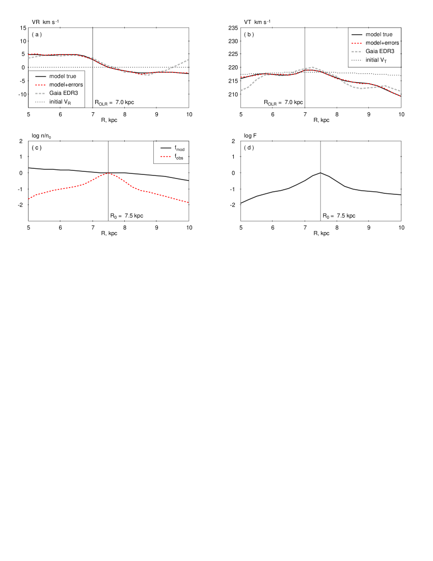
Figure 13: (a, b) Influence of observational errors onto the distribution of the velocities $V_{R}$ (a) and $V_{T}$ (b) along the distance $R$. The black solid lines describe the true velocity-profiles of model particles calculated in bins ($|\theta|<15^{\circ}$, $|z|<200$ pc, $\Delta R=250$ pc) while the red dashed lines indicate the velocity-profiles of model particles affected by random errors in parallaxes ($\sigma_{\varpi}=0.016$ mas), proper motions ($\sigma_{\mu}=0.015$ mas yr^-1) and line-of-sight velocities ($\sigma_{vr}=2.0$ km s^-1). We can see that observational errors have practically no effect on the velocity profiles in the distance interval $R=5$–10 kpc. Also shown are the velocity profiles computed for Gaia DR3 stars. (c, d) To study the effect of observational errors we simulated the spacial distribution of model particles close to the observed distribution. (c) Spacial distributions of model particles, $n$, in bins obtained for exponential discs ($f_{mod}$) and for Gaia DR3 stars ($f_{obs}$) normalized at the number of particles, $n_{0}$, located at the bin centered at the solar position ($R_{0}$=7.5 kpc). (d) Function $F=f_{mod}\;f_{obs}$ indicates the fraction of model particles which must be retained in each bin to mimic the selection effects in the distribution of Gaia DR3 stars with known line-of-sight velocities. Functions $f_{mod}$, $f_{obs}$ and $F$ are presented in logarithmic form.

References

- Arenou et al. (2018) Arenou, F., Luri, X., Babusiaux, C., et al., 2018, A&A, 616, 17
- Asano et al. (2020) Asano, T., Fujii, M. S., Baba, J., Bédorf, J., Sellentin, E., Portegies Zwart, S., 2020, MNRAS, 499, 2416
- Athanassoula (1992) Athanassoula E., 1992, MNRAS, 259, 328
- Athanassoula (2005) Athanassoula, E., 2005, MNRAS, 358, 1477
- Athanassoula et al. (1983) Athanassoula, E., Bienayme, O., Martinet, L., Pfenniger, D., 1983, A&A, 127, 349