Impact of magneto-rotational instability on grain growth in protoplanetary disks: II. Increased grain collisional velocities

Abstract

Turbulence is the dominant source of collisional velocities for grains with a wide range of sizes in protoplanetary disks. So far, only Kolmogorov turbulence has been considered for calculating grain collisional velocities, despite the evidence that turbulence in protoplanetary disks may be non-Kolmogorov. In this work, we present calculations of grain collisional velocities for arbitrary turbulence models characterized by power-law spectra and determined by three dimensionless parameters: the slope of the kinetic energy spectrum, the slope of the auto-correlation time, and the Reynolds number. The implications of our results are illustrated by numerical simulations of the grain size evolution for different turbulence models. We find that for the modeled cases of the Iroshnikov-Kraichnan turbulence and the turbulence induced by the magneto-rotational instabilities, collisional velocities of small grains are much larger than those for the standard Kolmogorov turbulence. This leads to faster grain coagulation in the outer regions of protoplanetary disks, resulting in rapid increase of dust opacity in mm-wavelength and possibly promoting planet formation in very young disks.

1. Introduction

Interstellar dust grains plays an important role in many aspects of astrophysics: they are building blocks of planets, commonly used gas tracer, and catalyst of molecular chemistry. All these processes depend on the size distribution of dust grains, and great efforts have been made to model the process of grain growth, especially in protoplanetary disks (see reviews by Blum & Wurm 2008; Testi et al. 2014; Birnstiel et al. 2016). In various astrophysical environments, turbulence is the major driving force for grain growth. Turbulent motions stir up the grains, leading to their mutual collisions. In protoplanetary disks, for example, turbulence is among the dominant sources for collisional velocities between grains in the size range of microns to meters (Birnstiel et al. 2011).

The calculation of grain collisional velocity induced by turbulence generally relies on one critical assumption: the turbulence is Kolmogorov with a kinetic energy spectrum of $E(k)\propto k^{-5/3}$. Völk et al. (1980) and Markiewicz et al. (1991) made the ground-laying work of calculating grain collisional velocities in Kolmogorov turbulence. Later Ormel & Cuzzi (2007, hereafter OC2007) derived the analytic expressions for grain collisional velocities in Kolmogorov turbulence, which were soon adopted in many grain coagulation codes (e.g. Brauer et al. 2008; Okuzumi et al. 2012; Akimkin et al. 2020b). The grain collisional velocities derived from these analytic Völk-type models were tested by direct numerical simulations in Pan & Padoan (2015); Ishihara et al. (2018) and Sakurai et al. (2021). The simulations showed that while Völk-type models suffer from several drawbacks, such as the neglect of turbulent clustering of same-size grains (which enhances their collisional rates) and a reduction of the rms collisional velocity (which reduce the collisional rates), the overall grain collisional velocities derived from Völk-type models are still accurate within a factor of $\sim 2$. With its relative accuracy and simplicity, the formulae in OC2007 remain the standard adopted in the current literature.

The astrophysical turbulence, however, does not necessarily have the Kolmogorov spectrum. The presence of magnetic fields is expected to change the turbulence cascade, and many alternative theories have been proposed to describe the magneto-hydrodynamic (MHD) turbulence. The Iroshnikov-Kraichnan (IK) theory, for example, predicts $E(k)\propto k^{-3/2}$ (Iroshnikov 1964; Kraichnan 1965). Alternatively, the Goldreich-Sridhar theory predicts $E(k_{\parallel})\propto k_{\parallel}^{-2}$ parallel to the mean magnetic field, and $E(k_{\perp})\propto k_{\perp}^{-5/3}$ perpendicular to the mean magnetic field (Goldreich & Sridhar 1995). These theories, however, assume that there is a dominant mean magnetic field. In many astrophysical environments such as the protoplanetary disks, the magnetic field is weak and the mean field varies on spatial and temporal scales of the turbulent cascade. It is unclear whether the theoretical predictions by the IK or Goldreich-Sridhar turbulence models still hold in these environments.

In our previous paper Gong et al. (2020, hereafter paperI), we preformed numerical simulations of the MHD turbulence in protoplanetary disks generated by the magneto-rotational instabilities (MRI). We observed a persistent kinetic energy spectrum of $k^{-4/3}$, which appears to be converged in terms of numerical resolution. This $k^{-4/3}$ energy spectrum has also been observed in many other MHD turbulence simulations in the literature (see Table 6 in paperI). To further investigate this phenomenon, we also performed driven turbulence simulations with and without the magnetic field and obtained the same energy spectrum. We concluded that the $k^{-4/3}$ power-law slope is likely due to the bottleneck effect near the dissipation scale of the turbulence (Ishihara et al. 2016). Due to the limited numerical resolution, we were not able to constrain whether the $k^{-4/3}$ energy spectrum extends to a larger dynamical range. In addition, we found the turbulence auto-correlation time to vary close to $\propto k^{-1}$, which is steeper than that for the Kolmogorov turbulence. Moreover, the injection scale of the MRI turbulence is determined by the fastest growing mode of the MRI – not by the scale-height of the disk assumed as the injection scale in OC2007. All these factors – the energy spectrum, the auto-correlation time and the injection scale of the turbulence – can have a big impact on the grain collisional velocities.

Recently, Grete et al. (2020) performed numerical simulations of weakly magnetized MHD turbulence, and found the same kinetic energy spectrum slope of $k^{-4/3}$. They analysed the energy transfer mechanisms in their simulations, and argued that magnetic tension must be the dominant force for energy transfer across scales. The energy transfer mechanism in Kolmogorov turbulence, the kinetic energy cascade, is suppressed in this case by the magnetic tension, to which they attributed the cause of the shallower $k^{-4/3}$ energy spectrum. Although they believe that the bottle-neck effect is not the cause of the $k^{-4/3}$ slope, their numerical resolution is still limited at $(2048)^{3}$. The power-law slope measured in Grete et al. (2020) spans within $\sim 2$ dex of the dissipation scale, where the bottle-neck effect is known to affect the energy spectrum (Ishihara et al. 2016). Moreover, there is no theoretical understanding so far about why the energy transfer by magnetic tension force may lead to the $k^{-4/3}$ energy spectrum. However, if the energy spectrum is indeed determined by the magnetic tension, the $k^{-4/3}$ slope can represent the inertial range of the turbulence cascade and extend to a much wider dynamic range far from the dissipation scale.

In addition, pure hydrodynamic instabilities can also generate turbulence in the protoplanetary disks in the absence of magnetic fields. For example, the subcritical baroclinic instability (SBI) driven by the radial entropy gradient (Klahr & Bodenheimer 2003; Klahr 2004; Petersen et al. 2007; Lesur & Papaloizou 2010), and the vertical shear instability (VSI) driven by the strong vertical shear (Nelson et al. 2013; Stoll & Kley 2016) can both generate long-lived turbulence in disks. Numerical simulations have found that the turbulence induced by the SBI or VSI can have much steeper kinetic energy spectra than the Kolmogorov turbulence across certain scales (Klahr & Bodenheimer 2003; Manger et al. 2020).

Given the uncertainty in the turbulence properties, this paper aims to provide insights into how non-Kolmogorov turbulence may affect grain collisional velocities and grain growth. In Section 2, we describe the turbulence models and the procedure for calculating the grain collisional velocities. We focus on three examples: the Kolmogorov turbulence, the IK turbulence, and the MRI turbulence described in paperI. The results are shown in Section 3. Section 3.1 derives the analytic approximation for the collisional velocities assuming a general case of power-law turbulence spectrum, and Section 3.2 compares the analytic approximation with accurate numerical integration. We also supply publicly available Python scripts that implemented our formulae for calculating the collisional velocities. Section 3.3 shows the dependence of grain collisional velocity on turbulence parameters, by describing its behavior in different limiting regimes. Section 4.1 presents an application of our work: we calculate grain growth in protoplanetary disks with different turbulence models, and estimate the fragmentation and drift barrier for grain growth due to non-Kolmogorov turbulence. Finally, Section 5 gives a summary of this work.

2. Method

We follow the method in Völk et al. (1980), Markiewicz et al. (1991) and OC2007 to calculate grain collisional velocities. These previous works considered only Kolmogorov turbulence. Here we generalize to a generic turbulence model with arbitrary power-law slopes of energy spectrum and auto-correlation time. We first describe the turbulence model, and then the steps to calculate the turbulence-induced grain collisional velocities. For the convenience of the reader, we summarize the important notations used in this paper in Table 1.

Table 1Summary of notations for the key physical variables

Symbol	Meaning
$\mathbf{v}$	gas velocity
$\delta\mathbf{v}$	$\mathbf{v}-\mathbf{v}_{K}$, turbulent gas velocity
$v_{\mathrm{tot}}$	large-scale turbulent velocity (Eq. (5))
$v_{\mathrm{rel}}(k)$	relative velocity between grain and eddy (Eq. (11))
$v_{p}\equiv\delta v_{p}$	turbulence induced grain velocity (Eq. (8))
$\Delta v_{12}$	collisional velocity between grain 1 and 2 (Eq. (18))
$\mathrm{St}$	Stokes number (Eq. (9))
$\mathrm{Re}$	Reynolds number (Eq. (2))
$\tau_{f}$	grain friction/stopping time (Eq. (8))
$\tau_{\mathrm{cross}}(k)$	eddy crossing time (Eq. (13))
$\tau(k)$	eddy auto-correlation time (Eq. (7))
$E(k)$	kinetic energy spectrum (Eq. (1))
$k_{L}$	injection scale (Fig. 1)
$k_{\eta}$	dissipation scale (Fig. 1)
$p$	power-law slope of $E(k)$
$m$	power-law slope of $\tau(k)$

2.1. Turbulence Model

There are two important properties of turbulence that determine the grain collisional velocities, the kinetic energy spectrum $E(k)$ and the eddy auto-correlation time $\tau(k)$. We assume the turbulence has a kinetic energy spectrum

$$E(k)=E_{L}\left(\frac{k}{k_{L}}\right)^{-p},\quad k_{L}\leq k\leq k_{\eta},$$ (1)

where $k_{L}$ and $k_{\eta}$ are the injection scale and dissipation scale of the turbulence. Outside of the range $k_{L}\leq k\leq k_{\eta}$, we simply assume $E(k)=0$.

The dissipation scale is determined by the Reynolds number,

$$\mathrm{Re}=\frac{vL}{\nu},$$ (2)

where $\nu$ is the viscosity, $v$ is the velocity, and $L$ is the length scale. Usually, the Reynolds number is defined for the largest turbulence eddy, $\mathrm{Re}=\mathrm{Re}(k_{L})=v(k_{L})L(k_{L})/\nu$. For turbulence eddy $k$, $v(k)=\sqrt{kE(k)}\propto k^{(1-p)/2}$, and $L(k)\propto 1/k$. At the dissipation scale, $\mathrm{Re}(k_{\eta})=v(k_{\eta})L(k_{\eta})/\nu=1$. This gives,

$$\mathrm{Re}=\frac{v(k_{L})L(k_{L})}{v(k_{\eta})L(k_{\eta})}=\left(\frac{k_{\eta}}{k_{L}}\right)^{(1+p)/2},$$ (3)

or equivalently,

$$\frac{k_{\eta}}{k_{L}}=\mathrm{Re}^{2/(1+p)}.$$ (4)

The large-scale (total) turbulent velocity $v_{\mathrm{tot}}$ is defined as

$$v_{\mathrm{tot}}^{2}=\int\mathrm{d}kE(k).$$ (5)

From the Plancherel theorem, $v_{\mathrm{tot}}^{2}=\langle v^{2}\rangle$, where $v$ is the magnitude of turbulent gas velocity and “$\langle~{}\rangle$” denotes the spacial average. Integrating Equation (5), we have

$$v_{\mathrm{tot}}^{2}=\frac{E_{L}k_{L}}{p-1}\left[1-\left(\frac{k_{\eta}}{k_{L}}\right)^{-(p-1)}\right]\approx\frac{E_{L}k_{L}}{p-1}.$$ (6)

For the integration to converge, it requires $p>1$.

The corresponding turbulent auto-correlation time in the inertial range is

$$\tau(k)=\tau_{L}\left(\frac{k}{k_{L}}\right)^{-m}.$$ (7)

Figure 1 illustrates the models for $E(k)$ and $\tau(k)$. For the detailed definitions of $E(k)$ and $\tau(k)$ see paperI.

Ormel & Cuzzi (2007) assumed $\tau(k)=1/(k\sqrt{2kE(k)})$ from the kinetic cascade, which gives $\tau_{L}=1/(k_{L}\sqrt{E_{L}k_{L}})$ and $m=(3-p)/2$. In paperI, we did observe that $\tau(k)\approx 1/(k\sqrt{2kE(k)})$ for the MRI as well as driven turbulence. In principle, $\tau(k)$ can be influenced also by other physical processes such as the interaction between the gas and the magnetic field. Without losing generality, we keep $p$ and $m$ as separate parameters. We focus on three turbulence models shown in Table 2, the Kolmogorov turbulence, the IK turbulence and the MRI turbulence in paperI. We note that our method can also be applied to other turbulence models with arbitrary values of $p$ and $m$.

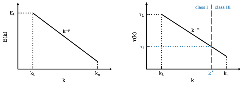
Figure 1.— Schematic diagrams of the kinetic energy spectrum $E(k)$ (left panel) and the eddy auto-correlation time $\tau(k)$ (right panel). $k_{L}$ and $k_{\eta}$ denote the injection and dissipation scales respectively. The blue annotations mark the transition between class I and class III eddies (see Equations (12) - (15))

Table 2Parameters for turbulence models considered in this work.

model	$p$	$m$	$(p-1)/m$
Kolmogorov	5/3	2/3	1
IK	3/2	3/4	2/3
paperI	4/3	5/6	2/5

2.2. Turbulence-induced Collisional Velocities

The dynamical property of a dust grain is characterized by its friction time (also often called the stopping time) $\tau_{f}$. The randomly fluctuating component of grain velocity $\delta\mathbf{v}_{p}$ follows (Equation (5) in Völk et al. 1980):

$$\frac{\mathrm{d}\delta\mathbf{v}_{p}}{\mathrm{d}t}=\frac{\delta\mathbf{v}-\delta\mathbf{v}_{p}}{\tau_{f}},$$ (8)

where $\delta\mathbf{v}$ is the random component of the gas velocity, such as the turbulent velocity in the protoplanetary disk. For the simplicity of notations, we hereafter drop the $\delta$ in Equation (8), and use $\mathbf{v}_{p}$ to denote the randomly fluctuating component of grain velocity induced by turbulence.

It is convenient to define the dimensionless Stokes number

$$\mathrm{St}=\tau_{f}/\tau_{L}.$$ (9)

Physically, $\tau_{f}$ or $\mathrm{St}$ is determined by the properties of both the grain and gas, and the relative velocity between them (Youdin 2010). For spherical grain in the Epstein drag regime (Epstein 1924), the friction time $\tau_{f}=\rho_{s}a/(\rho_{g}v_{\mathrm{th}})$, where $\rho_{s}$ and $a$ are the material density and radius of the grain, $\rho_{g}$ the gas density, and $v_{\mathrm{th}}$ the mean thermal velocity of the gas. In a protoplanetary disk, the Stokes number can be written as (Birnstiel et al. 2016),

$$\mathrm{St}=\frac{\pi}{2}\frac{\rho_{s}a}{\Sigma_{g}},$$ (10)

where $\Sigma_{g}$ is the gas surface density. Using the minimum mass solar nebular model (MMSN) in Hayashi (1981), $\mathrm{St}\approx 10^{-8}-1$ for typical grain sizes from $0.1~{}\mathrm{\mu m}$ to $1~{}\mathrm{cm}$ at $1-100~{}\mathrm{AU}$.

In this work, only perturbations from the gas motions on dust gains is considered, and the back reaction of dust grains onto the gas is ignored.

For two dust grains with friction times $\tau_{f1}$ and $\tau_{f2}$, their collisional velocity $\Delta v_{12}$ can be obtained by following the steps below:

1. Calculate the relative velocity $v_{\mathrm{rel}}(k)$ between the eddy $k$ and each dust grain (see Equation (19) in OC2007, ):

   $$v_{\mathrm{rel}}^{2}(k)=v_{\mathrm{sys}}^{2}+\int_{k_{L}}^{k}\mathrm{d}k^{\prime}E(k^{\prime})\left(\frac{\tau_{f}}{\tau_{f}+\tau(k^{\prime})}\right)^{2},$$ (11)

   where $v_{\mathrm{sys}}$ is the systematic velocity of the dust not driven by turbulence, such as the radial drift by pressure-gradient driven headwind or vertical settling due to the stellar gravity. Through out this work, we assume that the turbulent motions dominate and set $v_{\mathrm{sys}}=0$.

2. Determine the classes of eddies for each dust grain. The concept of “eddy classes” is first introduced by Völk et al. (1980). For a given dust grain with the friction time $\tau_{f}$ and a given eddy $k$, the eddy class is determined by

   $$\begin{cases}\tau_{f}<\mathrm{min}\{\tau(k),\tau_{\mathrm{cross}}(k)\},&\text{class {I} eddy}\\ \tau_{f}\geq\mathrm{min}\{\tau(k),\tau_{\mathrm{cross}}(k)\},&\text{class {III} eddy},\end{cases}$$ (12)

   where

   $$\tau_{\mathrm{cross}}(k)=\frac{1}{kv_{\mathrm{rel}}(k)}$$ (13)

   is the timescale on which the grain moves across the eddy. Grains are well-coupled with the class I eddies. This corresponds to small grains, for which $\tau_{f}$ is short enough that the grain “forgets” its initial motion and moves with the gas before it leaves the eddy or the eddy decays. On the contrary, grains are only weakly coupled with the class III eddies. Such grains are large enough that $\tau_{f}$ is long, and the eddy only exerts small perturbations to their motions. Because both $\tau(k)$ and $\tau_{\mathrm{cross}}(k)$ increase with $k$, a grain is better coupled with the large eddies than the small eddies. The transition scale between class I and class III eddies is defined as $k^{*}$: the eddies are class I for $k<k^{*}$ and class III for $k\geq k^{*}$. $k^{*}$ is a function of $\tau_{f}$ and can be solved by

   $$\mathrm{min}\{\tau(k^{*}),\tau_{\mathrm{cross}}(k^{*})\}=\tau_{f}.$$ (14)

   Appendix A shows that $k^{*}$ can be approximated using $\tau(k^{*})=\tau_{f}$. This gives,

   $$k^{*}=k_{L}\mathrm{St}^{-1/m}.$$ (15)

   Thus, there is no class I eddy for $\mathrm{St}\geq 1$, and no class III eddy for $\mathrm{St}\leq(k_{L}/k_{\eta})^{m}$ (see the right panel of Figure 1).

3. Calculate the velocity dispersion of each dust grain. The velocity dispersion of a dust grain induced by turbulence is given by Equation (6) in Markiewicz et al. (1991),

   $$\begin{split}v_{p}^{2}=&\int_{\textup{I}}\mathrm{d}kE(k)(1-K^{2})\\ &+\int_{\textup{III}}\mathrm{d}kE(k)(1-K)[g(\chi)+Kh(\chi)],\end{split}$$ (16)

   where $K=\tau_{f}/[\tau_{f}+\tau(k)]$, $g(\chi)=\chi^{-1}\arctan(\chi)$, $h(\chi)=1/(1+\chi^{2})$ and $\chi=K\tau(k)kv_{\mathrm{rel}}(k)$. Here I and III denotes the integration over class I ($k<k^{*}$) and class III ($k\geq k^{*}$) eddies.

4. Calculate the cross-correlation of the velocities between grains 1 and 2, $\langle\mathbf{v}_{p1}\cdot\mathbf{v}_{p2}\rangle$. From Markiewicz et al. (1991) Equation (8),

   $$\begin{split}\langle\mathbf{v}_{p1}\cdot\mathbf{v}_{p2}\rangle=&\frac{1}{\tau_{f1}+\tau_{f2}}\int_{\textup{I}_{12}}\mathrm{d}kE(k)\\ &\times[\tau_{f1}(1-K_{1}^{2})+\tau_{f2}(1-K_{2}^{2})],\end{split}$$ (17)

   where $\textup{I}_{12}$ denotes that the integration is over the eddies that are class I for both grain 1 and 2, i.e., $k<\mathrm{min}\{k_{1}^{*},k_{2}^{*}\}$.

5. Obtain the collisional velocity between grains 1 and 2. Finally, the collisional velocity $\Delta v_{12}$ can be calculated from

   $$(\Delta v_{12})^{2}=v_{p1}^{2}+v_{p2}^{2}-2\langle\mathbf{v}_{p1}\cdot\mathbf{v}_{p2}\rangle.$$ (18)

   For a given turbulence model, $(\Delta v_{12})^{2}$ is proportional to the total kinetic energy of the turbulence. Therefore, we usually present the normalized $\Delta v_{12}/v_{\mathrm{tot}}$ in the following sections.

3. Results

3.1. Analytic Approximations for Grain Collisional Velocities

We calculate the analytic approximations of grain collisional velocities in different regimes. The $k^{*}$ from Equation (15) is used to distinguish class I and class III eddies.

First, we calculate $v_{p}^{2}$ in Equation (16), which we divide into two terms, $v_{p}^{2}=T_{\textup{I}}+T_{\textup{III}}$,

$$T_{\textup{I}}=\int_{\textup{I}}\mathrm{d}kE(k)(1-K^{2}),$$ (19)

and

$$T_{\textup{III}}=\int_{\textup{III}}\mathrm{d}kE(k)(1-K)[g(\chi)+Kh(\chi)],$$ (20)

for the class I and class III eddies.

For the $T_{\textup{I}}$ term, there are two possible cases: (1) $\mathrm{St}\geq 1$. There is no class I eddy, and $T_{\textup{I}}=0$. (2) $\mathrm{St}<1$. In this case, for class I eddies $\tau_{f}\leq\tau(k)$, and thus we can approximate $1-K^{2}\approx 1-[\tau_{f}/\tau(k)]^{2}$. This gives,

$$\begin{split}T_{\textup{I}}(\mathrm{St})|_{k_{L}}^{k^{\prime}}&\approx\int_{k_{L}}^{k^{\prime}}\mathrm{d}kE(k)\left[1-\left(\frac{\tau_{f}}{\tau(k)}\right)^{2}\right]\\ &\approx v_{\mathrm{tot}}^{2}\left[1-\left(\frac{k_{L}}{k^{\prime}}\right)^{p-1}\right]\\ &-\frac{p-1}{1+2m-p}\mathrm{St}^{2}v_{\mathrm{tot}}^{2}\left[\left(\frac{k^{\prime}}{k_{L}}\right)^{1+2m-p}-1\right],\end{split}$$ (21)

where

$$k^{\prime}=\min\{k^{*},k_{\eta}\}.$$ (22)

$T_{\textup{I}}(\mathrm{St})|_{k_{L}}^{k^{\prime}}$ denotes the integration of the function $E(k)(1-K^{2})$ in the range of $k_{L}\leq k\leq k^{\prime}$ for a grain with Stokes number $\mathrm{St}$.

For the $T_{\textup{III}}$ term, we use the approximation $g(\chi)\approx h(\chi)\approx 1$, following OC2007. This gives $(1-K)[g(\chi)+Kh(\chi)]\approx 1-K^{2}\approx 2\tau(k)/\tau_{f}$, with $\tau(k)<\tau_{f}$ for class III eddies. There are 3 cases: (1) $\mathrm{St}\geq 1$. In this case, all eddies are class III, and

$$\begin{split}T_{\textup{III}}(\mathrm{St})|_{k_{L}}^{k_{\eta}}&\approx\int_{k_{L}}^{k_{\eta}}\mathrm{d}kE(k)\frac{2\tau(k)}{\tau_{f}}\\ &\approx\frac{2(p-1)}{p+m-1}\frac{v_{\mathrm{tot}}^{2}}{\mathrm{St}}\left[1-\left(\frac{k_{L}}{k_{\eta}}\right)^{p+m-1}\right].\end{split}$$ (23)

(2) $(k_{L}/k_{\eta})^{m}<\mathrm{St}<1$. Class III eddies have $k>k^{*}$, and

$$\begin{split}T_{\textup{III}}(\mathrm{St})|_{k^{*}}^{k_{\eta}}&\approx\int_{k^{*}}^{k_{\eta}}\mathrm{d}kE(k)\frac{2\tau(k)}{\tau_{f}}\\ &\approx\frac{2(p-1)}{p+m-1}\frac{v_{\mathrm{tot}}^{2}}{\mathrm{St}}\\ &\quad\times\left[\left(\frac{k_{L}}{k^{*}}\right)^{p+m-1}-\left(\frac{k_{L}}{k_{\eta}}\right)^{p+m-1}\right].\end{split}$$ (24)

(3) $\mathrm{St}\leq(k_{L}/k_{\eta})^{m}$. There is no class III eddies, and $T_{\textup{III}}=0$.

The cross correlation term in Equation (17) is only non-zero for two grains with $\mathrm{St}_{1}<1$ and $\mathrm{St}_{2}<1$. Assuming $\mathrm{St}_{2}<\mathrm{St}_{1}<1$, Equation (17) can be written as

$$\langle\mathbf{v}_{p1}\cdot\mathbf{v}_{p2}\rangle=\frac{\mathrm{St}_{1}}{\mathrm{St}_{1}+\mathrm{St}_{2}}T_{\textup{I}}(\mathrm{St}_{1})|_{k_{L}}^{k^{\prime}_{1}}+\frac{\mathrm{St}_{2}}{\mathrm{St}_{1}+\mathrm{St}_{2}}T_{\textup{I}}(\mathrm{St}_{2})|_{k_{L}}^{k^{\prime}_{1}},$$ (25)

where $k^{\prime}_{1}=\min\{k_{1}^{*},k_{\eta}\}$. The analytic approximation can be obtained from Equation (21).

3.2. Comparisons with Numerical Integrations

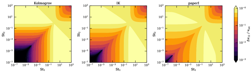
(a) Dust collisional velocities from numerical integrations.

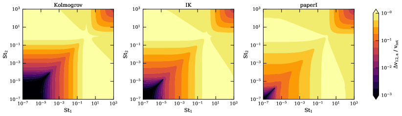
(b) Dust collisional veolcoties from analytic approximations.

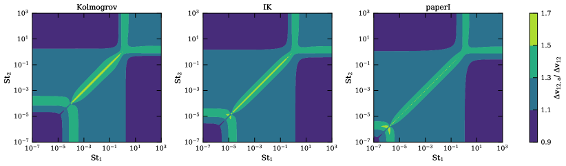
(c) The ratio between (b) and (a).

Figure 2.— Collisional velocities $\Delta v_{12}$ between two dust grains with stokes numbers $\mathrm{St_{1}}$ and $\mathrm{St_{2}}$, normalized by the total gas turbulent velocity $v_{\mathrm{tot}}$, in Kolmogorov (left), IK (middle) and paperI (right) turbulence models. (a) Collisional velocity $\Delta v_{12}$ from direct numerical integrations. (b) Collisional velocity $\Delta v_{12,a}$ from analytic approximations. (c) The ratio $\Delta v_{12,a}/\Delta v_{12}$.

The collisional velocities $\Delta v_{12}$ between two dust grains with Stokes numbers $\mathrm{St}_{1}$ and $\mathrm{St}_{2}$ in different turbulence models are shown in Figure 2, with Reynolds number $\mathrm{Re}=10^{8}$. The top panels show the collisional velocity from numerical integrations. In the regions where $\mathrm{St}_{1}\geq 1$ or $\mathrm{St}_{2}\geq 1$, the collisional velocities are very similar across different turbulence models. However, in the regions where $\mathrm{St}_{1},\mathrm{St}_{2}<1$, the collisional velocities can differ by orders of magnitude depending on the turbulence model. This behavior is explained in Section 3.3, where we derive the scaling relationship between $\Delta v_{12}$ and turbulence parameters.

The analytic approximation of $\Delta v_{12}$ is shown in the middle panels of Figure 2, and the differences between the analytic approximation and numerical integration are shown in the bottom panels. The analytic approximation is accurate within 30% in most regions and within 70% in all regions. The largest error occurs close to $\mathrm{St}=1$, $\mathrm{St}_{1}=\mathrm{St}_{2}$, and $\mathrm{St}=(k_{L}/k_{\eta})^{m}$, where the criteria for analytic approximations are not satisfied (see Section 3.1).

The analytic approximation allows for fast and accurate calculation of grain collisional velocities with arbitrary turbulence properties, without significant sacrifice in the accuracy. The analytic formulae in Section 3.1 can be easily implemented in grain growth codes, enabling the calculation of grain size evolution in non-Kolmogorov turbulence. We provide publicly available Python scripts that implemented our calculations at https://github.com/munan/grain_collision.

3.3. Limiting Behaviors

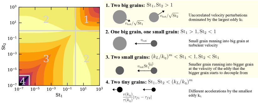
Figure 3.— The limiting behaviors of the grain collisional velocity $\Delta v_{12}$ in different regimes of the Stokes numbers. In regime 1 and 2, $\Delta v_{12}$ is dominated by the total turbulent velocity, and is insensitive to the turbulence properties. In regime 3 and 4, $\Delta v_{12}$ depends sensitively on the turbulence properties. The transition boundary between the two regimes and the grain collisional velocities are sensitive to the Reynolds number $\mathrm{Re}$, the power-law slope of the turbulence energy spectrum $p$, and power-law slope of the turbulence auto-correlation time $m$.

In order to obtain a clear physical understanding of the dependence of grain collisional velocities $\Delta v_{12}$ on the turbulence properties in Figure 2, we discuss the limiting behaviors of $\Delta v_{12}$. We divide the stokes numbers $\mathrm{St}_{1}$ and $\mathrm{St}_{2}$ into 4 regimes and discuss the dependence of $\Delta v_{12}$ on turbulence parameters in each regime. Figure 3 summarizes the limiting behaviors of $\Delta v_{12}$. Here we call the grains “big”, “small” or “tiny” defined by their Stokes numbers, which determine the scales of the turbulence eddies that they are coupled with. We always assume that the Reynolds number is large, and therefore $k_{L}/k_{\eta}\rightarrow 0$.

3.3.1 Two Big Grains

Take two big grains with $\mathrm{St}_{1}>1$ and $\mathrm{St}_{2}>1$: the eddies are all class III, and the cross term in Equation (17) vanishes. We can use Equation (23) to obtain,

$$\begin{split}(\Delta v_{12})^{2}&=v_{p1}^{2}+v_{p2}^{2}\\ &=T_{\textup{III}}(\mathrm{St}_{1})|_{k_{L}}^{k_{\eta}}+T_{\textup{III}}(\mathrm{St}_{2})|_{k_{L}}^{k_{\eta}}\\ &\approx\frac{2(p-1)v_{\mathrm{tot}}^{2}}{p+m-1}\left[1-\left(\frac{k_{L}}{k_{\eta}}\right)^{p+m-1}\right]\left(\frac{1}{\mathrm{St}_{1}}+\frac{1}{\mathrm{St}_{2}}\right)\\ &\approx v_{\mathrm{tot}}^{2}\left(\frac{1}{\mathrm{St}_{1}}+\frac{1}{\mathrm{St}_{2}}\right).\end{split}$$ (26)

The last step uses the approximation that the factor $2(p-1)/(p+m-1)$ is of order unity, and $k_{L}/k_{\eta}\ll 1$. In this case, each of the two grains are moving at an uncorrelated velocity of $v_{p}\approx v_{\mathrm{tot}}/\sqrt{\mathrm{St}}$. The velocity perturbation is dominated by the largest eddy.

3.3.2 One Big Grain and One Small Grain

Take one big grain with $\mathrm{St}_{1}>1$ and one small grain with $\mathrm{St}_{2}<1$: from Equations (19) and (20) we have,

$$\begin{split}(\Delta v_{12})^{2}&=v_{p1}^{2}+v_{p2}^{2}\\ &=T_{\textup{III}}(\mathrm{St}_{1})|_{k_{L}}^{k_{\eta}}+T_{\textup{I}}(\mathrm{St}_{2})|_{k_{L}}^{k^{\prime}_{2}}+T_{\textup{III}}(\mathrm{St}_{2})|_{k^{\prime}_{2}}^{k_{\eta}},\end{split}$$ (27)

where $k_{2}^{\prime}=\min\{k_{2}^{*},k_{\eta}\}$. In the limit of $\mathrm{St}_{1}\rightarrow\infty$ and $\mathrm{St}_{2}\rightarrow 0$, the terms $T_{\textup{III}}(\mathrm{St}_{1})|_{k_{L}}^{k_{\eta}}$ and $T_{\textup{III}}(\mathrm{St}_{2})|_{k^{\prime}_{2}}^{k_{\eta}}$ vanish. Following Equation (21),

$$(\Delta v_{12})^{2}\approx T_{\textup{I}}(\mathrm{St}_{2})|_{k_{L}}^{k^{\prime}_{2}}\approx v_{\mathrm{tot}}^{2}.$$ (28)

The bigger grain 1 barely moves due to its large mass, and the smaller grain 2 is well-coupled with the gas and moves at the turbulent velocity $v_{\mathrm{tot}}$.

3.3.3 Two Small Grains

Take two small grains with $(k_{L}/k_{\eta})^{m}<\mathrm{St}_{1}<1$ and $\mathrm{St}_{2}<\mathrm{St}_{1}$, we have

$$\begin{split}(\Delta v_{12})^{2}&=v_{p1}^{2}+v_{p2}^{2}-2\langle\mathbf{v}_{p1}\cdot\mathbf{v}_{p2}\rangle\\ &=T_{\textup{I}}(\mathrm{St}_{1})|_{k_{L}}^{k^{*}_{1}}+T_{\textup{III}}(\mathrm{St}_{1})|_{k^{*}_{1}}^{k_{\eta}}+T_{\textup{I}}(\mathrm{St}_{2})|_{k_{L}}^{k^{\prime}_{2}}\\ &\quad+T_{\textup{III}}(\mathrm{St}_{2})|_{k^{\prime}_{2}}^{k_{\eta}}-2\frac{\mathrm{St}_{1}}{\mathrm{St}_{1}+\mathrm{St}_{2}}T_{\textup{I}}(\mathrm{St}_{1})|_{k_{L}}^{k^{*}_{1}}\\ &\quad-2\frac{\mathrm{St}_{2}}{\mathrm{St}_{1}+\mathrm{St}_{2}}T_{\textup{I}}(\mathrm{St}_{2})|_{k_{L}}^{k^{*}_{1}}.\end{split}$$ (29)

We split the term $T_{\textup{I}}(\mathrm{St}_{2})|_{k_{L}}^{k^{\prime}_{2}}$ into two components, $T_{\textup{I}}(\mathrm{St}_{2})|_{k_{L}}^{k^{*}_{1}}+T_{\textup{I}}(\mathrm{St}_{2})|_{k^{*}_{1}}^{k^{\prime}_{2}}$, and neglect the second one compared to the first one, which allows us to approximate $T_{\textup{I}}(\mathrm{St}_{2})|_{k_{L}}^{k^{\prime}_{2}}\approx T_{\textup{I}}(\mathrm{St}_{2})|_{k_{L}}^{k^{*}_{1}}$. In addition, one can easily show that $T_{\textup{III}}(\mathrm{St}_{2})|_{k^{\prime}_{2}}^{k_{\eta}}<T_{\textup{III}}(\mathrm{St}_{1})|_{k^{*}_{1}}^{k_{\eta}}$, and therefore, the former term can be ignored. With these approximations, we write,

$$\begin{split}(\Delta v_{12})^{2}&\approx\frac{\mathrm{St}_{1}-\mathrm{St}_{2}}{\mathrm{St}_{1}+\mathrm{St}_{2}}[T_{\textup{I}}(\mathrm{St}_{2})-T_{\textup{I}}(\mathrm{St}_{1})]|_{k_{L}}^{k^{*}_{1}}+T_{\textup{III}}(\mathrm{St}_{1})|_{k^{*}_{1}}^{k_{\eta}}\\ &\approx\frac{(p-1)(\mathrm{St}_{1}-\mathrm{St}_{2})^{2}v_{\mathrm{tot}}^{2}}{1+2m-p}\left[\left(\frac{k^{*}_{1}}{k_{L}}\right)^{1+2m-p}-1\right]\\ &\quad+\frac{2(p-1)v_{\mathrm{tot}}^{2}}{(p+m-1)\mathrm{St}_{1}}\left(\frac{k_{L}}{k^{*}_{1}}\right)^{p+m-1}.\end{split}$$ (30)

If we take the limit of $\mathrm{St}_{2}\ll\mathrm{St}_{1}\ll 1$, then $k^{*}_{1}/k_{L}=\mathrm{St}_{1}^{-1/m}\gg 1$, giving

$$(\Delta v_{12})^{2}\approx v_{\mathrm{tot}}^{2}\mathrm{St}_{1}^{(p-1)/m}.$$ (31)

We can understand this scaling relation by considering the coupling of the dust grains with the gas: for eddies $k<k^{*}_{1}$, both grains are well-coupled with the gas, and the relative velocities are small. The collisional velocity is therefore dominated by the eddy $k^{*}_{1}$, where the larger grain 1 starts to decouple with the gas, and the smaller grain 2 is still well-coupled with the gas, running into the larger grain at the eddy velocity. The velocity of the eddy $k^{*}_{1}$ is,

$$v^{2}(k^{*}_{1})\sim k^{*}_{1}E(k^{*}_{1})\sim v_{\mathrm{tot}}^{2}\mathrm{St}_{1}^{(p-1)/m}.$$ (32)

Here the slope of the auto-correlation time $m$ determines the scale at which the larger grain starts to decouple, and the slope of the energy spectrum $p$ determines the eddy velocity at that scale.

3.3.4 Two tiny Grains

Take two tiny grains with $\mathrm{St}_{1},\mathrm{St}_{2}<(k_{L}/k_{\eta})^{m}$ and assuming $\mathrm{St}_{2}<\mathrm{St}_{1}$, all eddies are class I. Similar to Equation (30),

$$\begin{split}(\Delta v_{12})^{2}&\approx\frac{\mathrm{St}_{1}-\mathrm{St}_{2}}{\mathrm{St}_{1}+\mathrm{St}_{2}}[T_{\textup{I}}(\mathrm{St}_{2})-T_{\textup{I}}(\mathrm{St}_{1})]|_{k_{L}}^{k^{\eta}}\\ &\approx v_{\mathrm{tot}}^{2}\left(\frac{k_{\eta}}{k_{L}}\right)^{1+2m-p}(\mathrm{St}_{1}-\mathrm{St}_{2})^{2}\\ &\approx\left[\frac{v(k_{\eta})}{\tau(k_{\eta})}(\tau_{f1}-\tau_{f2})\right]^{2}.\end{split}$$ (33)

The collisional velocity is dominated by the smallest eddy $k_{\eta}$. The two grains of different sizes accelerate at different rates, causing the relative velocity. For grains with the exact same size, the collisional velocity is zero. The collisional velocity depends on the dissipation scale $k_{\eta}$, as well as the velocity and auto-correlation time of the eddy $k_{\eta}$. These are in turn determined by the Reynolds number, the energy spectrum slope $p$ and the slope of the auto-correlation time $m$.

4. Applications to Protoplanetary Disks

4.1. Grain Size Evolution

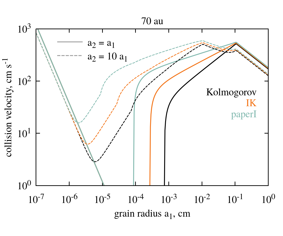
Figure 4.— Illustration of collision velocities between equal-size grains (solid lines) and grains with an order of magnitude size disparity (dashed lines). The results are for our three turbulence models (Kolmogorov, IK and paperI) at 70 au. For very small grains, the collisional velocity is dominated by the Brownian motion, which scales as $a^{-3/2}$. For larger grains, the collisional velocity is determined by turbulence, and can be approximately described by the 4 regimes discussed in Section 3.3. Consecutive transitions between regimes 4 through 1 (see Figure 3) are evident following the dashed lines ($a_{2}=10a_{1}$) as $a_{1}$ increases. For a wide range of grain sizes from sub-micron to millimeter, the collisional velocity is very sensitive to the turbulence properties.

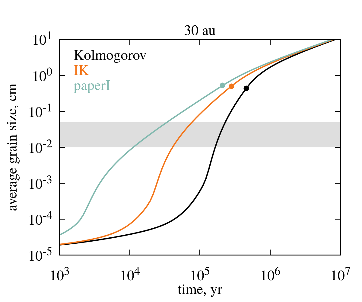
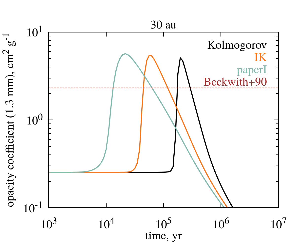
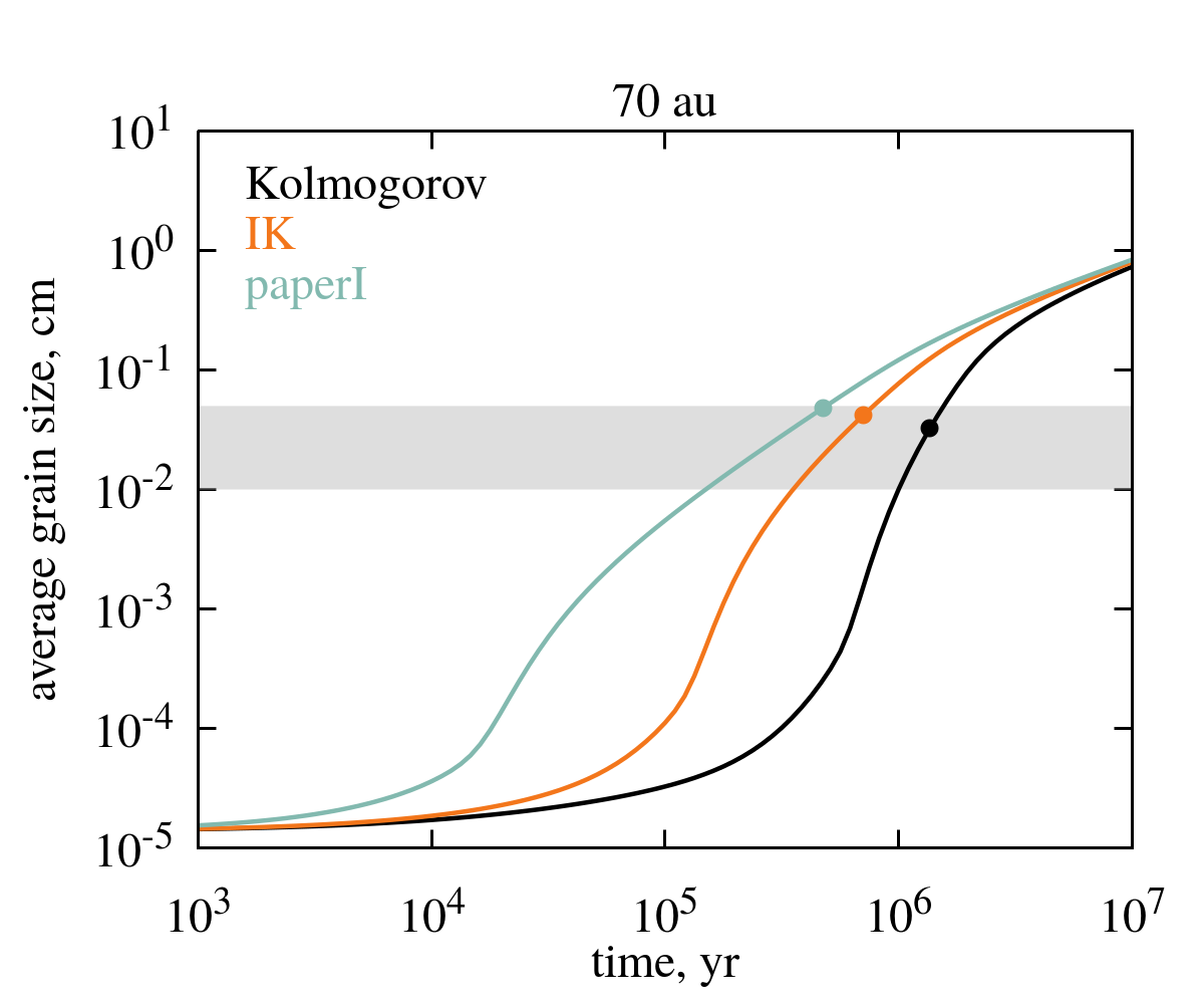
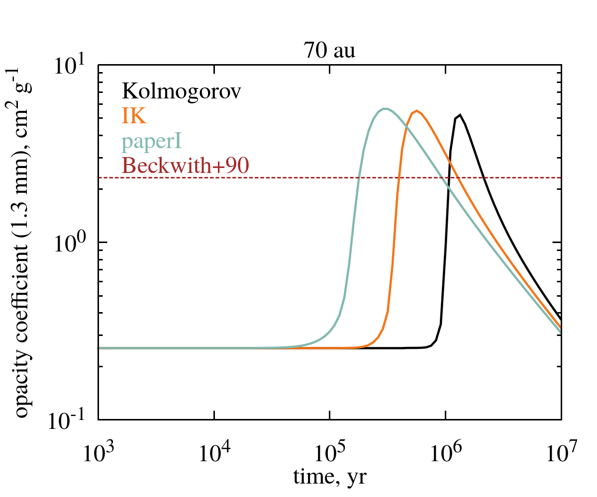
Figure 5.— Left: evolution of the average grain size (Equation (34)) in the disk mid-plane at 30 and 70 au. The gray shaded region marks the size-range which contributes the most to the dust emission at mm-wavelengths. The filled circles indicate radial drift barriers for each turbulence model according to Equation (40). Right: evolution of the dust opacity coefficient at the wavelength $\lambda=1.3$ mm (ALMA Band 6). The horizontal red dashed line shows the opacity coefficient of 2.3 cm² g^-1 in the observations by Beckwith et al. (1990).

Turbulence plays a crucial role in grain evolution in protoplanetary disks. It provides the dominant source of collisional velocities for micron- to centimeter- sized grains, which are too large to coagulate efficiently due to Brownian motion and too small to experience strong differential radial and azimuthal drift (Testi et al. 2014).

To show the impact of turbulence properties on grain evolution, we perform numerical simulations of grain coagulation in typical disk environments, similar to Akimkin et al. (2020b). We consider the simplest case of non-charged compact spherical grains with a material density of $\rho_{s}=3.0$ g cm^-3, a fixed dust-to-gas ratio of $\rho_{d}/\rho_{g}=0.01$, and a constant turbulence alpha-parameter of $\alpha=10^{-4}$. This low value of $\alpha$ is motivated by recent constrains by both dust and gas observations (Pinte et al. 2016; Flaherty et al. 2018), as well as from theoretical models (Simon et al. 2018). We take two sets of physical conditions in the disk: (1) $\rho_{g}=5\times 10^{-14}$ g cm^-3, $T_{g}=38$ K; and (2) $\rho_{g}=3\times 10^{-15}$ g cm^-3, $T_{g}=25$ K, where $\rho_{g}$ and $T_{g}$ are the gas density and temperature. These correspond to the conditions in the disk mid-plane at 30 and 70 au in Akimkin et al. (2020b). We choose to focus on the outer disk for the following reasons: (1) it is better probed by observations with its larger spacial scales and longer evolution time scales; and (2) the grain growth is less affected by fragmentation and radial drift, which we do not include in our model. In fact, for the parameter we choose, the maximum grain collisional velocity is $v_{\mathrm{coll}}\approx v_{\mathrm{tot}}\approx 4~{}\mathrm{m/s}$, smaller than the typical fragmentation velocity of $\sim 10~{}\mathrm{m/s}$ (Gundlach & Blum 2015). Using Equation (40) in Section 4.3, we calculated that the radial drift barrier occurs for grains of sizes $\approx 5$ mm at 30 au and $\approx 0.4$ mm at 70 au (marked by the filled circles in Figure 5). However, we note that the radial drift is very sensitive to the disk structure commonly observed (Andrews 2020; Segura-Cox et al. 2020). Non-smooth structures such as gaps and rings in the disk will significantly deter the drift.

The initial grain size distribution is taken to be a power-law with the slope of $-3.5$ in the range of $0.005-0.25~{}{\rm\mu}$m (Mathis et al. 1977). The coagulation equation is solved on a grid of grains masses ranging from $10^{-20}$ to $10^{7}$ g (roughly corresponding to sizes from $10^{-7}$ to $10^{2}$ cm) with 512 bins, providing resolution of $\sim 20$ bins per grain mass decade or $\sim 60$ bins per grain size decade.

We consider two sources of grain collisional velocities: the Brownian motion $\Delta v_{\rm Br}$ and turbulence-induced velocities $\Delta v_{12}$. The total grain collisional velocity is $\Delta v_{\rm coll}=\sqrt{(\Delta v_{\rm Br})^{2}+(\Delta v_{12})^{2}}$. In Figure 4 we show the collisional velocities between equal-size grains and grains with an order of size disparity, calculated at 70 au. The Brownian motion with $\Delta v_{\rm Br}\propto a^{-3/2}$ dominates for the smallest sizes. For $a$ near the transition to turbulence-driven motion, the resulting collision velocity exhibits a deep minimum, naturally leading to a slower coagulation for these sizes. This explains the small bump seen for micron-size grains in the size distribution (see the left panel of Figure 6 in Appendix B). For a large range of grain sizes from sub-micron to millimeter, the collisional velocity is very sensitive to the turbulence model, leading to dramatically different growth rates. To demonstrate the observational effect of different turbulence models on grain size evolution, we calculate the dust opacity coefficient $\kappa_{\nu}(t)=\int\pi a^{2}Q_{\rm abs}(a,\nu)f(m,t)\,{\rm d}m/\rho_{\rm d}$, where $f(m,t)$ is the grain mass distribution, $\rho_{\rm d}=\int mf(m,t)\,{\rm d}m$, and $Q_{\rm abs}(a,\nu)$ is the absorption efficiency obtained using the Mie theory for spherical silicate grains (Draine & Lee 1984; Akimkin et al. 2020a).

The left panels of Figure 5 show the evolution of the average grain radius for the three cases of turbulence models (Kolmogorov, IK, and paperI). The average grain radius $\bar{a}(t)$ is calculated from

$$\frac{4\pi}{3}\rho_{\rm s}\bar{a}^{3}(t)=\frac{\int m^{2}f(m,t)\,{\rm d}m}{\rho_{\rm d}}.$$ (34)

The corresponding dust opacity at the wavelength of 1.3 mm (ALMA Band 6) is illustrated in the right panels of Figure 5. The evolution of grain size distribution and dust opacity at 70 au is presented in Figure 6 in Appendix B. The evolution at 30 au is qualitatively similar to that at 70 au, but occurs faster due to the higher density and turbulent velocity. The higher collisional velocity for smaller grains in the IK and paperI turbulence makes their growth faster than in the standard Kolmogorov turbulence case. The size range of $0.1-0.5$ mm (gray shaded region in the left panels of Figure 5) is important, as such grains contribute the most to the disk millimeter emission (Rosotti et al. 2019; Akimkin et al. 2020a). This is also shown in the right panels of 5: as the average grain size increases, the 1.3 mm dust opacity first increases then decreases, peaking around the $0.1-0.5$ mm size-range. At 70 au, the grains grow to sub-millimeter sizes within 0.1 Myr with the paperI turbulence, while for the Kolmogorov turbulence, it takes 1 Myr to reach the same sizes.

The faster grain growth enabled by the non-Kolmogorov turbulence has interesting implications in many observational and theoretical aspects. This can result in rapid radial drift of dust grains in the outer disk, leading to the small disk sizes observed in class 0 and I protostars (Segura-Cox et al. 2016, 2018). Furthermore, it is known that grain charging may completely stop coagulation for micron-sized grains, especially for fluffy aggregates (Okuzumi 2009; Akimkin et al. 2020b). The higher collisional velocities provided by the IK and paperI turbulence can help to overcome this charge barrier. Generally, the faster grain growth provides more favorable conditions for early planet formation in young disks, by both accelerating the core formation processes and supplying solid material from the outer disk by the radial drift.

4.2. Fragmentation Barrier

We calculate the fragmentation barrier for grain growth following Birnstiel et al. (2012), but take into account the dependence of grain collisional velocities on turbulence properties. We estimate the collisional velocities of dust grains with $\mathrm{St}<1$ from Equation (31),

$$\Delta v_{\mathrm{coll}}\approx\sqrt{\alpha}c_{s}\mathrm{St}^{\frac{p-1}{2m}},$$ (35)

where $c_{s}$ is the sound speed. By equating $\Delta v_{\mathrm{coll}}$ to the fragmentation velocity $v_{\mathrm{frag}}$, we obtain the fragmentation barrier site,

$$a_{\mathrm{frag}}=\frac{\pi}{2}\frac{\Sigma_{g}}{\rho_{s}}\left[\frac{1}{\alpha}\left(\frac{v_{\mathrm{frag}}}{c_{s}}\right)^{2}\right]^{\frac{m}{p-1}}.$$ (36)

For Kolmogorov turbulence, where $m/(p-1)=1$, we recover Equation (8) in Birnstiel et al. (2012) within a pre-factor of order unity. For both the IK and paperI turbulence, the higher collisional velocities lead to smaller values of $a_{\mathrm{frag}}$ than that for the Kolmogorov turbulence. We note that the largest collisional velocity occurs for grains with $\mathrm{St}\approx 1$ (see Section 3.3) at $\Delta v_{\mathrm{coll}}\approx\sqrt{\alpha}c_{s}$. If $\sqrt{\alpha}c_{s}<v_{\mathrm{frag}}$, the fragmentation barrier is never reached (which is true for the cases considered in Section 4.1).

4.3. Radial Drift Barrier

Similar to the fragmentation barrier, the radial drift barrier also depends on the turbulence properties, which influences the grain growth timescale. From Birnstiel et al. (2012), the grain growth timescale is,

$$\tau_{\mathrm{grow}}=\frac{a\rho_{s}}{\rho_{d}\Delta v_{\mathrm{coll}}},$$ (37)

with the collisional velocity from Equation (35). The dust density $\rho_{d}$ is obtained from $\rho_{d}=\Sigma_{d}/(\sqrt{2\pi}h_{d})$, where the dust surface density is given by $\Sigma_{d}=\epsilon\Sigma_{g}$ with a constant dust to gas ratio $\epsilon=0.01$. The dust disk scale-height $h_{d}$ is calculated by Youdin & Lithwick (2007),

$$h_{d}=\sqrt{\frac{\alpha}{\mathrm{St}}}h_{g},$$ (38)

where $h_{g}$ is the gas disk scale-height. The drift timescale is,

$$\tau_{\mathrm{drift}}=\frac{rv_{k}}{\gamma\mathrm{St}c_{s}^{2}},$$ (39)

where $r$ is the disk radius and $\gamma=|\mathrm{d}\ln P/\mathrm{d}\ln r|$ is the absolute value of the power-law index of the gas pressure profile in the disk. From $\tau_{\mathrm{grow}}=\tau_{\mathrm{drift}}$, we obtain the drift barrier site,

$$a_{\mathrm{drift}}=\frac{2}{\pi}\frac{\Sigma_{g}}{\rho_{s}}\left[\left(\frac{\pi}{8}\right)^{1/2}\frac{\epsilon}{\gamma}\left(\frac{h_{g}}{r}\right)^{-2}\right]^{\frac{2m}{3m-p+1}}.$$ (40)

For Kolmogorov turbulence,

$$a_{\mathrm{drift,Kol}}=\frac{1}{\sqrt{2\pi}}\frac{\Sigma_{d}}{\rho_{s}\gamma}\left(\frac{h_{g}}{r}\right)^{-2},$$ (41)

which recovers the result from Equation (33) in Birnstiel et al. (2016). The values of $a_{\mathrm{drift}}$ are higher for the IK and paperI turbulence compared to that for the Kolmogorov turbulence, due to the higher collisional velocities and faster grain growth rates (Figure 5).

5. Summary

In this paper, we calculate of grain collisional velocities for an arbitrary turbulence model characterized by three dimensionless parameters: the slope of the kinetic energy spectrum $p$, the slope of the auto-correlation time $m$, and the Reynolds number $\mathrm{Re}$. Our work is a significant extension of calculations by OC2007, which being widely adopted in the literature, is only applicable to the Kolmogorov turbulence. As an example, we focus on three different turbulence models: the standard Kolmogorov turbulence, the IK model of MHD turbulence, and the MRI turbulence described in paperI. We calculate the grain collisional velocities using numerical integration. In addition, we derive accurate analytic approximations of the collisional velocities, and give scaling relations with the Stokes numbers and turbulence properties. To demonstrate the implications, we perform numerical simulations of the grain size evolution in the outer regions of protoplanetary disks, and calculate the fragmentation and radial drift barrier for grain growth in non-Kolmogorov turbulence models. The main findings of this paper are summarized as follows:

1. We calculate the grain collisional velocities between two dust grains in different turbulence models using both numerical integration and analytic approximations (Figure 2). The analytic approximation is simple and accurate, and can be readily implemented in complex numerical codes to model the grain size evolution in arbitrary turbulence models. We provide publicly available python scripts implementing our calculations at https://github.com/munan/grain_collision.

2. We introduce 4 characteristic regimes for the collisional velocities, depending on the Stokes numbers of the grains. We perform a detailed analysis of each regime, revealing the dominant mechanism that governs the collisional velocities and presenting the corresponding scaling relations (Figure 3). In particular, we show that the collisional velocities of small grains with $\mathrm{St}<1$ depend sensitively on the turbulence properties, with $(\Delta v_{12})^{2}\sim\mathrm{St}^{(p-1)/m}$ (Equation (31)).

3. The collisional velocity of small grains in IK and paperI turbulence are much higher (more than an order of magnitude for some grain sizes) than that in the Kolmogorov turbulence (Figure 4).

4. We perform numerical simulations of grain size evolution in the outer parts of protoplanetary disks. Compared to the Kolmogorov turbulence, the higher grain collisional velocities lead to faster grain growth in the IK and paperI turbulence models (Figure 5). For the MRI turbulence in paperI, grains can grow to sub-mm sizes within $\sim 0.1$ Myr even with a very low turbulence level ($\alpha=10^{-4}$) at 70 au. For Kolmogorov turbulence, growth to such sizes takes $\sim 1$ Myr.

5. The faster grain growth in the IK and paperI turbulence may lead to rapid increase of dust opacity at mm-wavelength (Figure 5). Increased collisional velocities can also help to overcome the charge barrier for the coagulation of micron-sized dust grains, accelerate the growth of pebbles and planetesimals, and thus promote planet formation in very young disks.

6. We calculate the fragmentation and drift barriers for grain growth in non-Kolmogorov turbulence (Equations (36) and (40)). Compared to the Kolmogorov turbulence, the higher grain collisional velocities for the IK and paperI turbulence lead to smaller values of $a_{\mathrm{frag}}$ and larger values of $a_{\mathrm{drift}}$.

In the future, our calculations can be implemented in numerical codes to explore the effect of non-Kolmogorov turbulence on the grain size evolution in a wide range of environments.

Appendix A Eddy Class

The eddy classes in Equation (12) is determined both by the auto-correlation time $\tau(k)=1/(kv(k))$ and the eddy crossing time $\tau_{\mathrm{cross}}(k)=1/(kv_{\mathrm{vel}}(k))$. Below we show that $v(k)\gtrsim v_{\mathrm{rel}}(k)$ for class I eddies, and hence $\tau(k)\lesssim\tau_{\mathrm{cross}}(k)$ in this case. Therefore, the transition scale $k^{*}$ can be calculated from the condition $\tau(k)=\tau_{f}$. There are three scenarios:

1. $\mathrm{St}\geq 1$. In this case $\tau_{f}>\tau_{L}$, and all eddies are class III.

2. $(k_{\eta}/k_{L})^{-m}<\mathrm{St}<1$. We define $k_{f}$ to be the scale where $\tau(k_{f})=\tau_{f}$, and thus $k_{f}/k_{L}=\mathrm{St}^{-1/m}$. Below we obtain that $v_{\mathrm{rel}}(k)$ is an increasing function of $k$ for $k\leq k_{f}$, whereas $\tau(k)$ always decreases with $k$. Therefore, for our purpose it is sufficient to show that $v(k_{f})\gtrsim v_{\mathrm{rel}}(k_{f})$.

   Because $\tau(k)\geq\tau_{f}$ at $k\leq k_{f}$, we can approximate $v_{\mathrm{rel}}(k)$ in Equation (11) with,

   $$\begin{split}v_{\mathrm{rel}}^{2}(k_{f})&\approx\int_{k_{L}}^{k_{f}}\mathrm{d}kE(k)\left(\frac{\tau_{f}}{\tau(k)}\right)^{2}\\ &=k_{L}E_{L}\mathrm{St}^{2}\int_{1}^{k_{f}/k_{L}}x^{2m-p}\mathrm{d}x\\ &\approx\frac{p-1}{2m+1-p}v_{\mathrm{tot}}^{2}\mathrm{St}^{2}\left(\frac{k_{f}}{k_{L}}\right)^{2m+1-p}\\ &=\frac{p-1}{2m+1-p}v_{\mathrm{tot}}^{2}\mathrm{St}^{(p-1)/m}.\end{split}$$ (A1)

   To approximate the integration, the second last step of used the fact that $2m+1-p>1$ for the turbulence models we considered (Table 2) as well as $k_{f}/k_{L}>1$.

   For $v(k)$, we have

   $$v^{2}(k_{f})=2k_{f}E(k_{f})=2k_{L}E_{L}\left(\frac{k_{f}}{k_{L}}\right)^{1-p}=2(p-1)v_{\mathrm{tot}}^{2}\mathrm{St}^{(p-1)/m}.$$ (A2)

   Comparing Equations (A1) and (A2), we obtain $v(k_{f})\gtrsim v_{\mathrm{rel}}(k_{f})$, and thus $\tau(k_{f})\lesssim\tau_{\mathrm{cross}}(k_{f})$. This gives $k^{*}\approx k_{f}$ and thus

   $$k^{*}\approx k_{L}\mathrm{St}^{-1/m}.$$ (A3)

3. $\mathrm{St}\leq(k_{\eta}/k_{L})^{-m}$. In this last case, we compare $v_{\mathrm{rel}}(k_{\eta})$ to $v(k_{\eta})$. From Equation (A1), we have

   $$\begin{split}v_{\mathrm{rel}}^{2}(k_{\eta})&\approx\frac{1}{2m+1-p}k_{L}E_{L}\mathrm{St}^{2}\left(\frac{k_{\eta}}{k_{L}}\right)^{2m+1-p}\\ &\leq\frac{p-1}{2m+1-p}v_{\mathrm{tot}}^{2}\left(\frac{k_{\eta}}{k_{L}}\right)^{-(p-1)},\end{split}$$ (A4)

   and similar to Equation (A2),

   $$v^{2}(k_{\eta})=2(p-1)v_{\mathrm{tot}}^{2}\left(\frac{k_{\eta}}{k_{L}}\right)^{-(p-1)}\\ .$$ (A5)

   This gives $v(k_{\eta})\gtrsim v_{\mathrm{rel}}(k_{\eta})$ and $\tau(k_{\eta})\lesssim\tau_{\mathrm{cross}}(k_{\eta})$, similar to the previous case. In this case, all eddies are class I.

Appendix B Grain Size Distribution and Opacity Coefficients

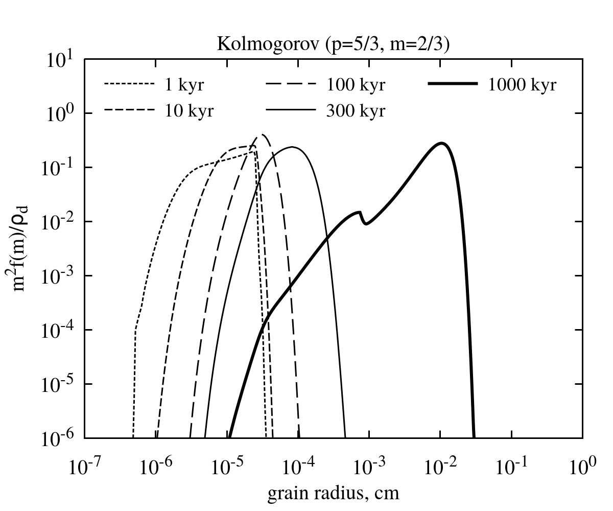
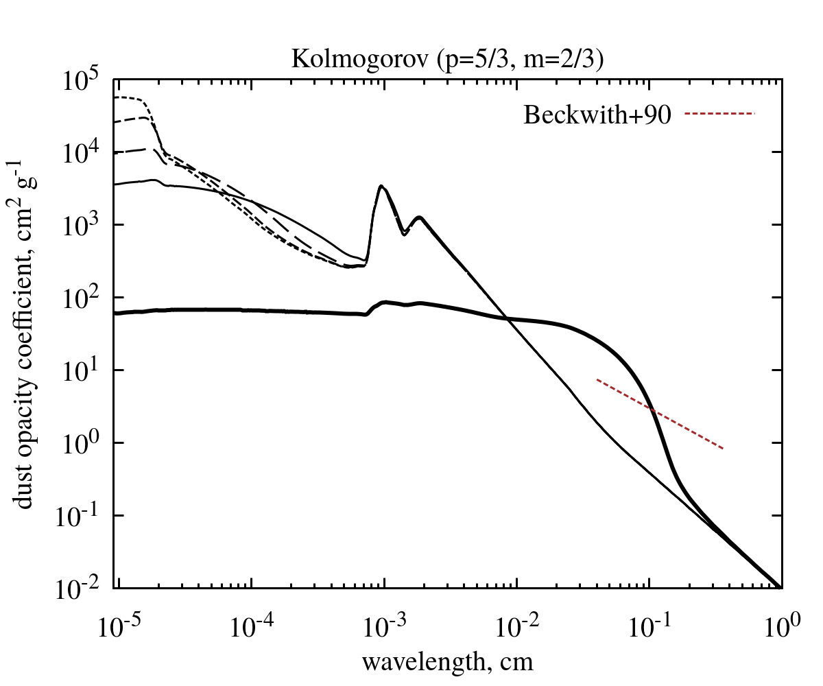
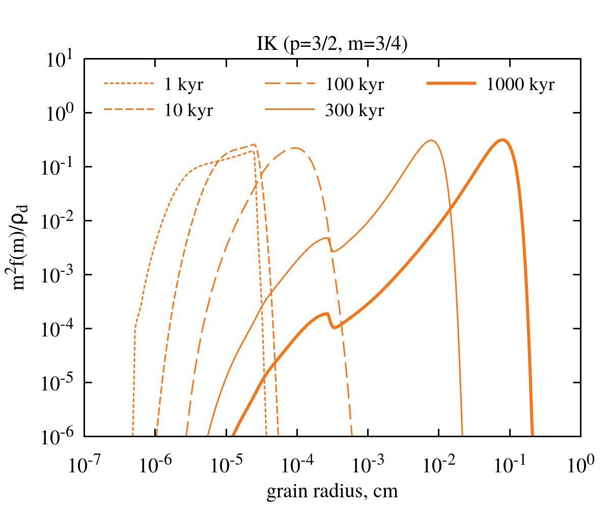
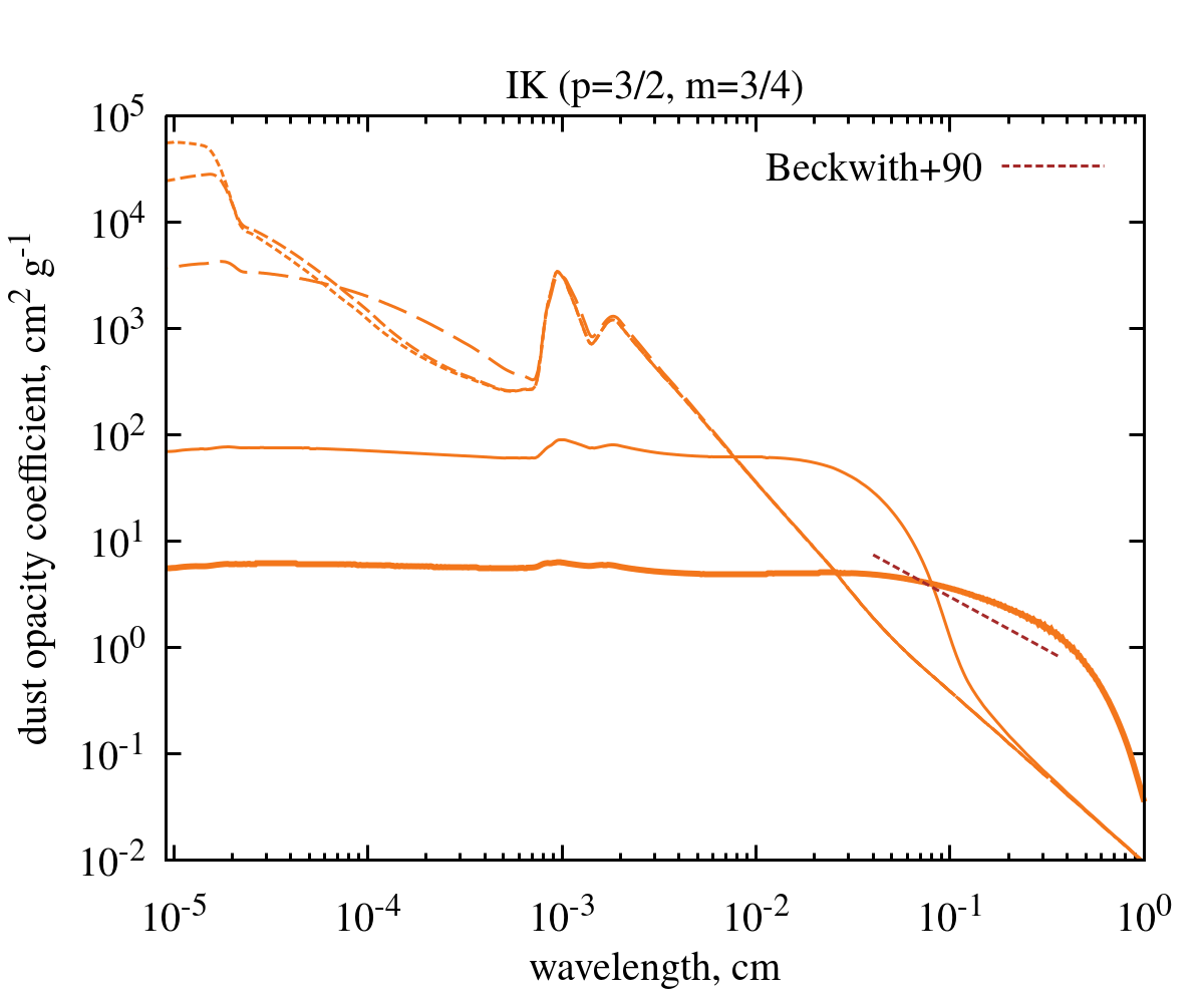
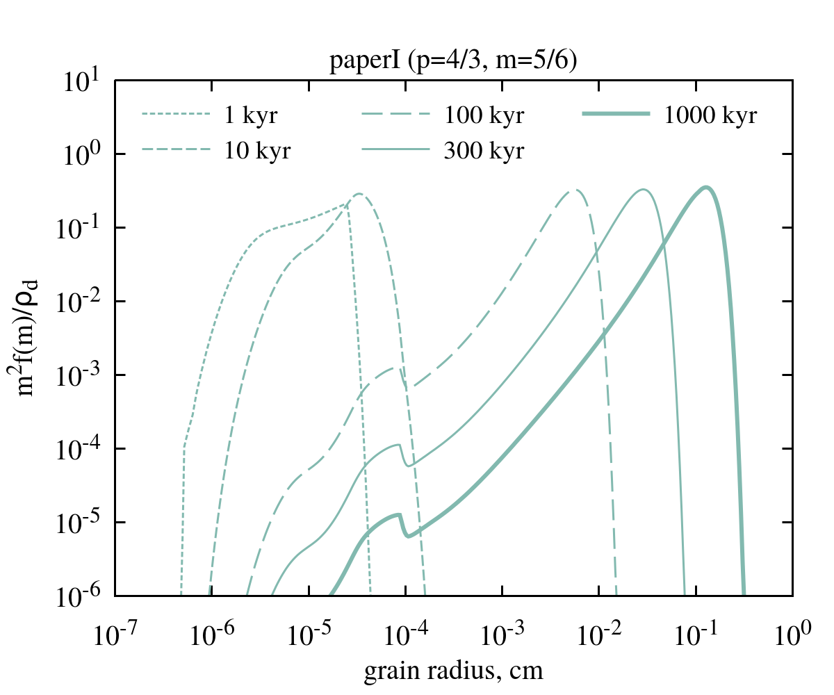
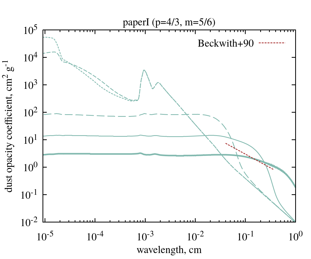
Figure 6.— Evolution of the grain size distribution (left) and the corresponding opacity coefficients (right) in the disk mid-plane at 70 au. The Kolmogorov, IK and paperI turbulence cases are shown in the top, middle and bottom panels. The red dashed lines in the right panels indicate the the opacity coefficients in the mm-wavelength range by Beckwith et al. (1990).

Figure 6 shows the evolution of the grain size distribution and wavelength-dependent dust opacity coefficients at 70 au for the Kolmogorov, IK and paperI turbulence models. The early evolution at $t\lesssim 10^{4}~{}\mathrm{yr}$ is governed by the Brownian motion, and therefore insensitive to the turbulence properties. Higher turbulence-induced collisional velocities in the paperI case (see Figure 4) push the peak of the grain size distribution to $\sim 100~{}{\rm\mu}$m already at $10^{5}$ yr, giving rise to an earlier increase of dust opacities in the millimeter wavelength range.

References

- Akimkin et al. (2020a) Akimkin, V., Vorobyov, E., Pavlyuchenkov, Y., & Stoyanovskaya, O. 2020a, MNRAS, 499, 5578
- Akimkin et al. (2020b) Akimkin, V. V., Ivlev, A. V., & Caselli, P. 2020b, ApJ, 889, 64
- Andrews (2020) Andrews, S. M. 2020, ARA&A, 58, 483
- Beckwith et al. (1990) Beckwith, S. V. W., Sargent, A. I., Chini, R. S., & Guesten, R. 1990, AJ, 99, 924
- Birnstiel et al. (2016) Birnstiel, T., Fang, M., & Johansen, A. 2016, Space Sci. Rev., 205, 41
- Birnstiel et al. (2012) Birnstiel, T., Klahr, H., & Ercolano, B. 2012, A&A, 539, A148
- Birnstiel et al. (2011) Birnstiel, T., Ormel, C. W., & Dullemond, C. P. 2011, A&A, 525, A11
- Blum & Wurm (2008) Blum, J., & Wurm, G. 2008, ARA&A, 46, 21
- Brauer et al. (2008) Brauer, F., Dullemond, C. P., & Henning, T. 2008, A&A, 480, 859
- Draine & Lee (1984) Draine, B. T., & Lee, H. M. 1984, ApJ, 285, 89
- Epstein (1924) Epstein, P. S. 1924, Phys. Rev., 23, 710
- Flaherty et al. (2018) Flaherty, K. M., Hughes, A. M., Teague, R., et al. 2018, ApJ, 856, 117
- Goldreich & Sridhar (1995) Goldreich, P., & Sridhar, S. 1995, ApJ, 438, 763
- Gong et al. (2020) Gong, M., Ivlev, A. V., Zhao, B., & Caselli, P. 2020, ApJ, 891, 172
- Grete et al. (2020) Grete, P., O’Shea, B. W., & Beckwith, K. 2020, arXiv e-prints, arXiv:2009.03342
- Gundlach & Blum (2015) Gundlach, B., & Blum, J. 2015, ApJ, 798, 34
- Hayashi (1981) Hayashi, C. 1981, Progress of Theoretical Physics Supplement, 70, 35
- Iroshnikov (1964) Iroshnikov, P. S. 1964, Soviet Ast., 7, 566
- Ishihara et al. (2018) Ishihara, T., Kobayashi, N., Enohata, K., Umemura, M., & Shiraishi, K. 2018, ApJ, 854, 81
- Ishihara et al. (2016) Ishihara, T., Morishita, K., Yokokawa, M., Uno, A., & Kaneda, Y. 2016, Phys. Rev. Fluids, 1, 082403
- Klahr (2004) Klahr, H. 2004, ApJ, 606, 1070
- Klahr & Bodenheimer (2003) Klahr, H. H., & Bodenheimer, P. 2003, ApJ, 582, 869
- Kraichnan (1965) Kraichnan, R. H. 1965, Physics of Fluids, 8, 1385
- Lesur & Papaloizou (2010) Lesur, G., & Papaloizou, J. C. B. 2010, A&A, 513, A60
- Manger et al. (2020) Manger, N., Klahr, H., Kley, W., & Flock, M. 2020, MNRAS, 499, 1841
- Markiewicz et al. (1991) Markiewicz, W. J., Mizuno, H., & Voelk, H. J. 1991, A&A, 242, 286
- Mathis et al. (1977) Mathis, J. S., Rumpl, W., & Nordsieck, K. H. 1977, ApJ, 217, 425
- Nelson et al. (2013) Nelson, R. P., Gressel, O., & Umurhan, O. M. 2013, MNRAS, 435, 2610
- Okuzumi (2009) Okuzumi, S. 2009, ApJ, 698, 1122
- Okuzumi et al. (2012) Okuzumi, S., Tanaka, H., Kobayashi, H., & Wada, K. 2012, ApJ, 752, 106
- Ormel & Cuzzi (2007) Ormel, C. W., & Cuzzi, J. N. 2007, A&A, 466, 413
- Pan & Padoan (2015) Pan, L., & Padoan, P. 2015, ApJ, 812, 10
- Petersen et al. (2007) Petersen, M. R., Julien, K., & Stewart, G. R. 2007, ApJ, 658, 1236
- Pinte et al. (2016) Pinte, C., Dent, W. R. F., Ménard, F., et al. 2016, ApJ, 816, 25
- Rosotti et al. (2019) Rosotti, G. P., Tazzari, M., Booth, R. A., et al. 2019, MNRAS, 486, 4829
- Sakurai et al. (2021) Sakurai, Y., Ishihara, T., Furuya, H., Umemura, M., & Shiraishi, K. 2021, ApJ, 911, 140
- Segura-Cox et al. (2016) Segura-Cox, D. M., Harris, R. J., Tobin, J. J., et al. 2016, ApJ, 817, L14
- Segura-Cox et al. (2018) Segura-Cox, D. M., Looney, L. W., Tobin, J. J., et al. 2018, ApJ, 866, 161
- Segura-Cox et al. (2020) Segura-Cox, D. M., Schmiedeke, A., Pineda, J. E., et al. 2020, Nature, 586, 228
- Simon et al. (2018) Simon, J. B., Bai, X.-N., Flaherty, K. M., & Hughes, A. M. 2018, ApJ, 865, 10
- Stoll & Kley (2016) Stoll, M. H. R., & Kley, W. 2016, A&A, 594, A57
- Testi et al. (2014) Testi, L., Birnstiel, T., Ricci, L., et al. 2014, in Protostars and Planets VI, ed. H. Beuther, R. S. Klessen, C. P. Dullemond, & T. Henning, 339
- Völk et al. (1980) Völk, H. J., Jones, F. C., Morfill, G. E., & Roeser, S. 1980, A&A, 85, 316
- Youdin (2010) Youdin, A. N. 2010, in EAS Publications Series, Vol. 41, EAS Publications Series, ed. T. Montmerle, D. Ehrenreich, & A. M. Lagrange, 187–207
- Youdin & Lithwick (2007) Youdin, A. N., & Lithwick, Y. 2007, Icarus, 192, 588