Equivalence of a harmonic oscillator to a free particle and Eisenhart lift

Abstract

It is widely known in quantum mechanics that solutions of the Schrödinger equation (SE) for a linear potential are in one-to-one correspondence with the solutions of the free SE. The physical reason for this correspondence is Einstein’s principle of equivalence. What is usually not so widely known is that solutions of the Schrödinger equation with harmonic potential can also be mapped to the solutions of the free Schrödinger equation. The physical understanding of this equivalence is not known as precisely as in the case of the equivalence principle. We present a geometric picture that will link both of the above equivalences with one constraint on the Eisenhart metric.

1 Introduction

There is no clear-cut answer to the question of what geometry is, since “the meaning of the word geometry changes with time and with the speaker” [1]. Classical mechanics was closely related to geometry from the very beginning. During the time of Newton and Huygens, many mechanical arguments were very geometrical, leading to extensive use of Euclidean geometry. Then came the period when more attention began to be paid to analytical methods, and Lagrange even boasted that his treatise on analytical mechanics did not contain any pictures [2]. The subsequent development of classical mechanics revealed the importance of both analytical and geometric methods. The role of geometric ideas and the corresponding intuition became especially evident after the works of Poinceré and Birkhoff. However, the geometries underlying Hamiltonian mechanics were a new kind of geometry, namely symplectic geometry and its odd-dimensional cousin contact geometry [2, 3, 4, 5]

With the advent of Einstein’s general theory of relativity, the role of geometry in fundamental physics has increased significantly. General relativity has two essential features. The first decisive step is the transition from three-dimensional Euclidean geometry to four-dimensional spacetime geometry by incorporating time as the fourth coordinate, and this has already been done by Minkowski in the context of special relativity. The second key step is to interpret gravity as the curvature of this four-dimensional pseudo-Riemannian spacetime geometry.

Since Einstein’s time, this geometrization of physics has advanced enormously. In classical physics, all Standard Model fundamental interactions are closely linked with suitably generalized notions of curvature in geometry. Quantum theory adds global (topological) aspects to this local picture of connections between physics and geometry. As a result, quite diverse, interesting, and unexpected geometrical and topological results have emerged from the interactions of modern mathematics with fundamental physics [8].

Modern differential geometry can be described as the study of (smoothly varying) tensor structures on the tangent bundle. In Riemannian geometry, the structure is defined in terms of a symmetric, positive definite second rank tensor, in contact geometry, in terms of a nondegenerate one-form, and in symplectic geometry, in terms of a nondegenerate two-form [9].

If we understand geometrization of nonrelativistic classical mechanics in a narrower sense as geometrization through Riemannian or Lorentzian (pseudo-Riemannian) geometry, we have two options: the “intrinsic” approach of Cartan and the “ambient” approach of Eisenhart [10, 11]. In fact, the two approaches are deeply interrelated [10, 12].

Eisenhart [13] made a very important contribution to the geometrization of nonrelativistic mechanics. This approach, commonly known as the Eisenhart lift, was rediscovered by Duval and coworkers [12] in a slightly different geometric context of Bargmann structures. Eisenhart showed that trajectories of a holonomic conservative dynamical system can be considered as null-projections (shadows) of geodesics of some ambient Lorentzian spacetime, in amusing analogy with Plato’s cave [11]. These ambient spacetimes are in fact gravitational waves with parallel rays, first considered by Brinkmann in a different context [14, 15]. However, Brinkmann did not notice any connection with nonrelativistic physics. Be that as it may, historically, neither the results of Eisenhart nor Brinkmann actually influenced the development of contemporary physics in any way, since they went largely unnoticed and then forgotten [10].

This connection between nonrelativistic and relativistic physics allows one to borrow techniques from one field to another, especially the powerful geometric tools of Lorentzian geometry. For example, the study of symmetries of a nonrelativistic system can be viewed as isometries of the Eisenhart metric. Interesting results were obtained in this way [16, 17, 18].

Duval and his colleagues extended Eisenhart results to nonrelativistic quantum mechanics [12], which opened the way for many applications (see, for example, [10, 11, 19, 20] and references therein), including applications to the nonrelativistic version of the AdS/CFT correspondence [21, 22], and to the Wheeler-DeWitt equation [23].

One of the features of the Eisenhart lift is that the potential term of nonrelativistic physics turns into a component of the corresponding Eisenhart metric. We can use other coordinates to describe this Brinkman wave and change the metric tensor according to the corresponding coordinate transformation. When we null-project this new metric back to a nonrelativistic level, we get the Schrödinger equation with a different potential. Thus, with the help of the Eisenhart lift, it is possible to find correspondences between the physics of two different physical systems, determined by different potentials.

In this article, we investigate such mappings for the class of potentials giving a flat Lorentzian metric after the Eisenhart lift. In section II, we briefly review the Eisenhart lift to the extent required for the purposes of this study. Next, we will find the flatness condition for the Eisenhart metric, which will restrict the choice of the potential. The resulting class of potentials and the corresponding equivalencies are explored in the subsequent sections.

2 Eisenhart Lift

In this section, we’ll take a very brief look at the basics of the Eisenhart lift. For a more detailed discussion of the material, see [11, 12, 13, 16, 17, 24, 25, 26], and for a curious analogy to Plato’s cave see [27].

Consider a general dynamical system described by the Lagrangian

$$L\left(x,\dot{x},t\right)=\frac{1}{2}\,g_{ij}\frac{dx^{i}}{dt}\frac{dx^{j}}{dt}+A_{i}\left(x,t\right)\frac{dx^{i}}{dt}-V\left(x,t\right),$$ (1)

where $g_{ij}$ is the so-called mass matrix, and $A_{i}$, $V$ are analogous to the vector and scalar potentials of the electromagnetic system. To have a benign nonrelativistic system, we assume that the kinetic term is a positive-definite quadratic form in the velocities. In (1), the time $t$ is an evolution parameter that is not part of the configuration-space manifold. To transform it into a coordinate on the manifold $(x^{i},t)$ and, thus, treat it on an equal footing with the spatial coordinates $x^{i}$, we introduce (in the general case, non-integrable) local time $\tau$ as follows:

$$m\,d\tau=\Omega\left(x,t\right)dt,$$ (2)

where $m$ is a constant, and its introduction reflects the fact that local clocks parameterize trajectories only up to a linear transformation ($m$ reflects the arbitrariness in the choice of time units) [28].

Note that (2) can be viewed as a generalized Sundman transformation [29, 30]. Alternatively, in the spirit of the theory of relativity, we can interpret $\tau$ as the local time measured by an arbitrary observer along his/her world-line, and then $\Omega$ will serve as the conversion factor to Newtonian absolute time $t$.

As a result the Lagrangian now becomes

$$L=\Omega(x,t)\left\{\frac{1}{2}\,g_{ij}\frac{dx^{i}}{d\tau}\frac{dx^{j}}{d\tau}+A_{i}\frac{dx^{i}}{d\tau}\frac{dt}{d\tau}-V\frac{dt}{d\tau}\frac{dt}{d\tau}\right\}$$ (3)

The above Lagrangian is obtained by rewriting the action integral in terms of the local time $\tau$ and taking into account the fact that the classical action is defined up to a multiplicative constant. We still cannot interpret the above Lagrangian as a geodesic Lagrangian for the metric

$$d\bar{s}^{2}=\Omega\left(x,t\right)\left[g_{ij}dx^{i}dx^{j}+2A_{i}dx^{i}dt-2Vdt^{2}\right],$$ (4)

since $\tau$ is not an affine parameter, as it is normalized by $\Omega\frac{dt}{d\tau}=m$, and not by the usual normalization condition, which is $g_{\mu\nu}\frac{dx^{\mu}}{d\tau}\frac{dx^{\nu}}{d\tau}=\mathrm{constant}$.

To correct this deficiency, we introduce a new coordinate $u$ such that [11]

$$du=-Ldt-\frac{M^{2}}{m}\,d\tau,$$ (5)

where $M$ is some constant. Then

$$2\,dudt=-\left(g_{ij}dx^{i}dx^{j}+2A_{i}dx^{i}dt-2Vdt^{2}\right)-2\,\frac{M^{2}}{m}d\tau dt=$$ (6)

$$-\left(g_{ij}dx^{i}dx^{j}+2A_{i}dx^{i}dt-2Vdt^{2}\right)-\Omega\,\frac{M^{2}}{m^{2}}dt^{2}-\frac{M^{2}}{\Omega}d\tau^{2},$$

where we have used (2) to rewrite the last term in the first line in an equivalent form.

After using the above tricks, our final metric becomes

$$ds^{2}=-M^{2}d\tau^{2}=$$

$$\Omega\left(x,t\right)\left\{g_{ij}dx^{i}dx^{j}+2A_{i}dx^{i}dt+2dtdu-2\left(V-\frac{M^{2}}{2m^{2}}\,\Omega\right)dt^{2}\right\},$$ (7)

or

$$ds^{2}=-M^{2}d\tau^{2}=g_{\mu\nu}dx^{\mu}dx^{\nu},$$ (8)

and now it is clear that the parameter $\tau$ is normalized in the usual way and therefore can be considered as an affine parameter. In (8) $x^{\mu}=(t,u,x^{i})$, $i=1,2,...n$ are coordinates on a $n+2$ dimensional Lorentzian manifold.

Thus, the generalized Sundman factor $\Omega$ turns out to be the conformal factor relating the ambient metric (7) to the conformally equivalent metric

$$d\tilde{s}^{2}=g_{ij}dx^{i}dx^{j}+2A_{i}(x,t)dx^{i}dt+2dtdu-2U(x,t)dt^{2},$$ (9)

with

$$U(x,t)=V(x,t)-\frac{M^{2}}{2m^{2}}\,\Omega(x,t).$$ (10)

The ambient metric (7) was first obtained by Lichnerowicz [32], and the metric (7), without the conformal factor $\Omega$, was obtained by Eisenhart [13]. Obviously, the conformal factor allows one to significantly enlarge the class of the Eisenhart-lifted metrics. As we will see later in this article, it is exactly this conformal factor that will allow us to find the equivalence of the harmonic oscillator to a free particle in the classical and quantum contexts.

The usefulness of the ambient metric (7) becomes apparent from the following Eisenhart-Lichnerowicz theorem [11]:

Let $\tau$ be an affine parameter such that $\frac{dt}{d\tau}\neq 0$ and $g_{\mu\nu}\frac{dx^{\mu}(\tau)}{d\tau}\frac{dx^{\nu}(\tau)}{d\tau}=-M^{2}$ on a manifold endowed with the metric

$$ds^{2}=\Omega\left(x,t\right)\left\{g_{ij}dx^{i}dx^{j}+2A_{i}dx^{i}dt+2dtdu-2Udt^{2}\right\}.$$

Then the geodesic equation for a curve $x^{\mu}(\tau)=\left(t(\tau),u(\tau),x^{i}(\tau)\right)$, when projected along the direction of $u$ reduces to the Euler-Lagrange Equation of the nonrelativistic holonomic dynamical system with the Lagrangian $L=\dfrac{1}{2}\,g_{ij}\frac{dx^{i}}{dt}\frac{dx^{j}}{dt}+A_{i}\frac{dx^{i}}{dt}-V$, where $V=U+\frac{M^{2}}{2m^{2}}\,\Omega$, with $m=\Omega\,\frac{dt}{d\tau}$.

3 Flatness conditions

For one space dimension, that is, $x^{\mu}=(t,u,x)$, and for $A_{i}=0$ we get the ambient metric as

$$ds^{*2}=\Omega\left(x,t\right)\left\{g(x,t)dx^{2}+2dtdu-2Udt^{2}\right\}.$$ (11)

We want the corresponding Riemann curvature tensor to vanish, which will give us flat metric conditions for the potential $U(x,t)$ and the conformal factor $\Omega\left(x,t\right)$.

For our purposes, we further specialize to the case $g=1$. If the metric (11) is flat, then the metric

$$ds^{2}=dx^{2}+2dtdu-2Udt^{2}$$ (12)

is conformally flat. On the other hand, it is well known that in the three-dimensional case, a necessary and sufficient condition for the metric to be conformally flat is the vanishing of the Cotton tensor [33, 34]. In terms of the Ricci tensor $R_{\mu\nu}$ and the scalar curvature $R$, the three-dimensional Cotton tensor has the form

$$C_{\mu\nu\lambda}=\nabla_{\lambda}R_{\mu\nu}-\nabla_{\nu}R_{\mu\lambda}+\frac{1}{4}\left(g_{\mu\lambda}\nabla_{\nu}R-g_{\mu\nu}\nabla_{\lambda}R\right).$$ (13)

For the metric (12), the non-zero Christoffel symbols of the first kind are

$$\Gamma_{ttt}=-\frac{\partial U}{\partial t},\;\;\Gamma_{ttx}=\Gamma_{txt}=-\frac{\partial U}{\partial x},\;\;\Gamma_{xtt}=\frac{\partial U}{\partial x}.$$ (14)

Using the inverse metric for (12),

$$g^{\mu\nu}=\left(\begin{array}[]{ccc}0&1&0\\ 1&2U&0\\ 0&0&1\end{array}\right),$$ (15)

we find the non-zero Christoffel symbols of the second kind

$$\Gamma^{x}_{\;tt}=\frac{\partial U}{\partial x},\;\;\Gamma^{u}_{\;tx}=\Gamma^{u}_{\;xt}=-\frac{\partial U}{\partial x},\;\;\Gamma^{u}_{\;tt}=-\frac{\partial U}{\partial t}.$$ (16)

To calculate the curvature, it is useful to use Cartan’s structure equation (see, for example, [39, 40])

$${\bf R}^{\mu}_{\;\nu}=d{\bf\Gamma}^{\mu}_{\;\nu}+{\bf\Gamma}^{\mu}_{\;\sigma}\wedge{\bf\Gamma}^{\sigma}_{\;\nu},$$ (17)

where (we use bold to indicate differential forms) ${\bf\Gamma}^{\mu}_{\;\nu}=\Gamma^{\mu}_{\;\nu\lambda}\,dx^{\lambda}$ are connection 1-forms, and ${\bf R}^{\mu}_{\;\nu}=\frac{1}{2}\,R^{\mu}_{\nu\lambda\sigma}dx^{\lambda}\wedge dx^{\sigma}$ are curvature 2-forms.

From (16) we find non-zero connection 1-forms

$${\bf\Gamma}^{x}_{\;t}=\frac{\partial U}{\partial x}dt,\;\;{\bf\Gamma}^{u}_{\;x}=-\frac{\partial U}{\partial x}dt,\;\;{\bf\Gamma}^{u}_{\;t}=-\frac{\partial U}{\partial t}dt-\frac{\partial U}{\partial x}dx,$$ (18)

and using (17) we find that there are only two non-zero curvature 2-forms:

$${\bf R}^{x}_{\;t}=\frac{\partial^{2}U}{\partial x^{2}}\,dx\wedge dt,\;\;\;{\bf R}^{u}_{\;x}=-\frac{\partial^{2}U}{\partial x^{2}}\,dx\wedge dt.$$ (19)

Therefore, for the metric (12), non-zero independent components of the Riemann curvature tensor are

$$R^{x}_{txt}=\frac{\partial^{2}U}{\partial x^{2}},\;\;\;R^{u}_{xxt}=-\frac{\partial^{2}U}{\partial x^{2}}.$$ (20)

As a result, the Ricci tensor has only one non-zero component, and the scalar curvature vanishes (since $g^{tt}=0$):

$$R_{tt}=\frac{\partial^{2}U}{\partial x^{2}},\;\;\;R=g^{\mu\nu}R_{\nu\mu}=0.$$ (21)

We now have all the ingredients for computing the Cotton tensor using (13). The only non-zero components turn out to be

$$C_{ttx}=-C_{txt}=\frac{\partial^{3}U}{\partial x^{3}}.$$ (22)

As we see, a necessary and sufficient condition for the metric (12) to be conformally flat is

$$\frac{\partial^{3}U(x,t)}{\partial x^{3}}=0.$$ (23)

If two metrics are conformally related $g_{\mu\nu}^{*}=e^{2\sigma}g_{\mu\nu}$, when the corresponding curvature tensors are related as follows [33]:

$$e^{-2\sigma}R^{*}_{\mu\nu\lambda\tau}=R_{\mu\nu\lambda\tau}+g_{\mu\tau}\sigma_{\nu\lambda}+g_{\nu\lambda}\sigma_{\mu\tau}-g_{\mu\lambda}\sigma_{\nu\tau}-g_{\nu\tau}\sigma_{\mu\lambda}+\left(g_{\mu\tau}g_{\nu\lambda}-g_{\mu\lambda}g_{\nu\tau}\right)\Delta_{1}\sigma,$$ (24)

where

$$\sigma_{\mu\nu}=\nabla_{\mu}\nabla_{\nu}\sigma-(\nabla_{\mu}\sigma)(\nabla_{\nu}\sigma)=\nabla_{\mu}(\partial_{\nu}\sigma)-(\partial_{\mu}\sigma)(\partial_{\nu}\sigma),$$

$$\Delta_{1}\sigma=g^{\mu\nu}(\nabla_{\mu}\sigma)(\nabla_{\nu}\sigma)=g^{\mu\nu}(\partial_{\mu}\sigma)(\partial_{\nu}\sigma).$$ (25)

Since $R_{tutu}=g_{tt}R^{t}_{utu}+g_{tu}R^{u}_{utu}=0$, $g_{uu}=0$ and $\sigma$ does not depend on $u$, (25) indicates that when the metric (11) is flat we will have

$$\Delta_{1}\sigma=g^{xx}\left(\frac{\partial\sigma}{\partial x}\right)^{2}=\left(\frac{\partial\sigma}{\partial x}\right)^{2}=0.$$ (26)

Therefore, when the Eisenhart metric (11) is flat, the local time (2) is integrable, since $\sigma$ (and thus $\Omega$) is independent of $x$.

The conformal transformation law for the three-dimensional Ricci tensor is [33, 41, 42] (note that in [33] the Ricci tensor is defined with the opposite sign)

$$R^{*}_{\mu\nu}=R_{\mu\nu}-\sigma_{\mu\nu}-g_{\mu\nu}\left(\Delta_{2}\sigma+\Delta_{1}\sigma\right),\;\;\;\Delta_{2}\sigma=g^{\mu\nu}\nabla_{\mu}\nabla_{\nu}\sigma=g^{\mu\nu}\nabla_{\mu}\left(\partial_{\nu}\sigma\right).$$ (27)

As we have seen, the only non-zero component of the Ricci tensor is $R_{tt}$. Since $\sigma$ does not depend on $x$, (15) indicates that both $\Delta_{2}\sigma$ and $\Delta_{1}\sigma$ are zero, and as a flatness condition we get $R_{tt}=\sigma_{tt}=\partial_{t}\partial_{t}\sigma-(\partial_{t}\sigma)^{2}$ (we have taken into account that $\nabla_{t}(\partial_{t}\sigma)=\partial_{t}\partial_{t}\sigma-\Gamma^{x}_{tt}\,\partial_{x}\sigma-\Gamma^{u}_{tt}\,\partial_{u}\sigma=\partial_{t}\partial_{t}\sigma$).

In terms of $\Omega=e^{2\sigma}$ the flatness conditions takes the form

$$\frac{\partial\Omega}{\partial x}=0,\;\;\;\frac{\partial^{2}U}{\partial x^{2}}=\frac{1}{\Omega^{2}}\left\{\frac{\Omega}{2}\,\frac{\partial^{2}\Omega}{\partial t^{2}}-\frac{3}{4}\left(\frac{\partial\Omega}{\partial t}\right)^{2}\right\}.$$ (28)

Note that (23) follows from (28), so (28) is a necessary and sufficient condition the metric (11) (with $g=1$) to be flat. In addition, as $\Omega$ is $x$-independent, it follows from (10) that $\frac{\partial^{2}U}{\partial x^{2}}=\frac{\partial^{2}V}{\partial x^{2}}$, and the conditions (28) do not depend on $M$. In particular, we can take $M=0$, which corresponds to null-geodesics in the ambient spacetime. Accordingly, in what follows we replace $U$ by $V$.

Thus, under our assumptions, we finally obtain a class of potentials for which the Eisenhart metric (11) is flat, or, in other words, the metric can be brought to the standard Minkowski form by means of a suitable coordinate transformation. It is somewhat surprising that only spatially linear, or quadratic potentials are allowed by the flatness condition, while there is still huge scope for temporal dependence. Nevertheless, the Eisenhart metric (11) allows to analyze interesting cases such as harmonic oscillator (both time-dependent and time-independent), linear potential etc.

For further analysis, it is useful to introduce a function $\Phi(t)$ such that $\Omega=\frac{d\Phi}{dt}$ and rewrite the second equation in (28) in the form

$$\frac{\partial^{2}V}{\partial x^{2}}=\frac{1}{2}\,S_{t}(\Phi),\;\;\;S_{t}(\Phi)=\frac{1}{\frac{d\Phi}{dt}}\frac{d^{3}\Phi}{dt^{3}}-\frac{3}{2}\frac{1}{\left(\frac{d\Phi}{dt}\right)^{2}}\left(\frac{d^{2}\Phi}{dt^{2}}\right)^{2}.$$ (29)

Here $S_{t}(\Phi)$ is the so-called Schwarzian derivative of the function $\Phi(\tau)$. Despite its rather complicated form, the Schwarzian derivative is ubiquitous and tends to appear in many seemingly unrelated fields of mathematics [43, 44, 45].

Now, since we have a metric that is flat under condition (29), we will try to find a coordinate transformation that brings this metric

$$ds^{*2}=\Omega\left(t\right)\left\{dx^{2}+2dtdu-2Vdt^{2}\right\}.$$ (30)

to the standard Minkowski form. It can be checked rather easily that the transformation $(t,u,x)\rightarrow(\tau,v,\xi)$, with

$$x=f_{1}\left(\xi,\tau\right),\;\;\;t=f_{2}\left(\xi,\tau\right),\;\;u=v+f_{3}\left(\xi,\tau\right),$$ (31)

brings the metric (30) in the Minkowski form $ds^{*2}=d\xi^{2}+2d\tau dv$ if

$$\frac{\partial f_{1}}{\partial\xi}=\frac{1}{\sqrt{\Omega(t)}},\;\frac{df_{2}}{d\tau}=\frac{1}{\Omega(t)},\;\frac{\partial f_{2}}{\partial\xi}=0,$$

$$\left(\frac{\partial f_{1}}{\partial\tau}\right)^{2}+\frac{2}{\Omega(t)}\,\frac{\partial f_{3}}{\partial\tau}-\frac{2V}{\Omega(t)^{2}}=0,\;\sqrt{\Omega(t)}\;\frac{\partial f_{1}}{\partial\tau}+\frac{\partial f_{3}}{\partial\xi}=0.$$ (32)

It is clear from the second and third equations in (32) that $t=f_{2}(\tau)$ is a function of $\tau$ only. This function can be found by inverting the relation $\tau=\int\Omega(t)dt$ and then the system (32) has a solution

$$x=f_{1}\left(\xi,\tau\right)=\frac{\xi}{\sqrt{\Omega(t)}}+h\left(\tau\right),\;\;\;f_{3}\left(\xi,\tau\right)=\frac{\xi^{2}}{4\Omega(t)}\frac{d\Omega(t)}{d\tau}-\sqrt{\Omega(t)}\;\frac{dh}{d\tau}\,\xi+p\left(\tau\right),$$ (33)

where the functions $p(\tau)$ and $h(\tau)$ are constrained by the fourth equation in (32). In particular, for this equation to be valid for all values of $\tau$ and $\xi$, the functions $p(\tau)$ and $h(\tau)$ must satisfy the equations

$$\frac{dp}{d\tau}=-\frac{\Omega(t)}{2}\left(\frac{dh}{d\tau}\right)^{2}+\frac{S_{t}[\Phi]\,h^{2}}{4\Omega(t)}+\frac{B(t)\,h}{\Omega(t)}+\frac{C(t)}{\Omega(t)},$$ (34)

and

$$\frac{d^{2}h}{d\tau^{2}}+\frac{1}{\Omega(t)}\,\frac{d\Omega(t)}{d\tau}\,\frac{dh}{d\tau}+\frac{S_{t}[\Phi]\,h}{2\Omega^{2}(t)}=-\frac{B(t)}{\Omega^{2}(t)}.$$ (35)

To derive the above equations, we used the most general form of the potential, compatible with (29):

$$V(x,t)=\frac{1}{4}S_{t}(\Phi)x^{2}+B(t)x+C(t).$$ (36)

Here $B(t)$ and $C(t)$ are arbitrary functions of time.

Equations (33)-(35) constitute the required coordinate transformation for the potential (36). Different choices of the potential $V(x,t)$ correspond to different forms of $S_{t}(\Phi(t))$, from which we get $\Phi(t)$ and hence $\Omega(t)$. Then, in principle, we can find the function $t(\tau)$, solve the differential equation (35) for $h(\tau)$ and then determine $p(\tau)$ from (34). Finally, we get the required coordinate transformation using (33).

Let us see how the nonrelativistic Lagrangian $L_{V}=\frac{1}{2}\left(\frac{dx}{dt}\right)^{2}-V(x,t)$ is related to the free Lagrangian $L_{free}=\frac{1}{2}\left(\frac{d\xi}{d\tau}\right)^{2}$. We have

$$\frac{dx}{dt}=\Omega(t)\left[\frac{\partial f_{1}}{\partial\xi}\,\frac{d\xi}{d\tau}+\frac{\partial f_{1}}{\partial\tau}\right]=\sqrt{\Omega(t)}\left[\frac{d\xi}{d\tau}+\sqrt{\Omega(t)}\,\frac{\partial f_{1}}{\partial\tau}\right],$$

and using relations from (32), we get

$$\frac{1}{2}\left(\frac{dx}{dt}\right)^{2}=\Omega(t)\left[\frac{1}{2}\left(\frac{d\xi}{d\tau}\right)^{2}-\frac{\partial f_{3}}{\partial\tau}-\frac{d\xi}{d\tau}\,\frac{\partial f_{3}}{\partial\xi}\right]+V(x,t)=$$

$$\Omega(t)\left[\frac{1}{2}\left(\frac{d\xi}{d\tau}\right)^{2}-\frac{df_{3}}{d\tau}\right]+V(x,t).$$

Therefore, $L_{V}=\Omega(t)\left[L_{free}-\frac{df_{3}}{d\tau}\right]$ and we see that the Lagrangian does not remain invariant under transformations (33). However, the actions $S_{V}=\int L_{V}dt$ and $S_{free}=\int L_{free}\,d\tau$ are equivalent. Indeed,

$$S_{V}=\int\limits_{t_{i}}^{t_{f}}L_{V}dt=\int\limits_{t_{i}}^{t_{f}}{\Omega(t)\left[L_{free}-\frac{df_{3}}{d\tau}\right]}dt,$$ (37)

and using $d\tau=\Omega(t)dt$ from (32), we get

$$S_{V}=\int\limits_{\tau_{i}}^{\tau_{f}}{\left[L_{free}-\frac{df_{3}}{d\tau}\right]}d\tau=S_{free}-\left[f_{3}\left(\xi(\tau_{f}),\tau_{f}\right)-f_{3}\left(\xi(\tau_{i}),\tau_{i}\right)\right].$$ (38)

The boundary terms in square brackets do not affect Euler-Lagrange equations of motion.

The quantity $e^{iS}$, which is central in the path-integral formulation of quantum mechanics, when the coordinates change according to (33), transforms as $e^{iS_{V}}\rightarrow e^{-if_{3}}e^{iS_{free}}$. Thus, $f_{3}$ is a phase factor. Although the transformation of the Eisenhart metric is purely classical, it is surprising that it can generate a quantum mechanical phase factor. This hints at the possibility that the Eisenhart lift can also incorporate quantum transformations, with the auxiliary coordinate $u$ acting as a phase factor. In the next section, we will find out exactly how the wave functions are transformed when the coordinates change according to (33), and we will show that the function $f_{3}$ is indeed a phase factor accompanying the transformation of the wave function.

4 Schrödinger Equation and Eisenhart lift

It is known that the Schrödinger equation can be derived as a null dimensional reduction of the Klein-Gordon equation [11, 12]. This connection has interesting applications because the Eisenhart metric (7) (called Platonic waves in [11]) covers a large class of spacetimes of physical and mathematical importance [11]. After the null dimensional reduction, various Eisenhart metrics will correspond to different potentials in the Schrödinger equation. For example, a class of spacetimes, called AdS-pp-waves, can be obtained using $\Omega=\frac{1}{x^{2}}$ and arbitrary scalar potential $V(x,t)$ in (30). Further specialization $V\sim-x^{2\left(1-Z\right)},\;Z\geq 1$ gives us the so called Schrödinger spacetime. Anti-de Sitter spacetime corresponds to $Z=1$.

Interestingly, the Schrödinger spacetimes have applications to nonrelativistic holography [46]. Another important observation is that in [47] Penrose proved that near a null geodesic, every Lorentzian spacetime looks like a pp-wave with metric which is exactly the Eisenhart metric in two spatial dimensions with $\Omega=1$ and $V=a(t)(x^{2}-y^{2})+2b(t)xy$ for some $a(t)$, $b(t)$. This result is known as the Penrose limit in the physical literature [48].

Since Eisenhart metric covers such a wide class of important manifolds, the study of the quantum field theory in these Eisenhart spacetimes is expected to be significantly simplified by converting the problem to the corresponding Schrödinger equation. On the contrary, the understanding of the corresponding Schrödinger equation can help in the study of Eisenhart spacetimes. Below this correspondence between the Eisenhart metric and the Schrödinger equation is illustrated in the context of the flat Eisenhart metric (30).

Let $x^{\mu}=(t,u,x)$, and consider the Klien-Gordon equation of a massless scalar field $\phi$ in the 3-dimensional Eisenhart metric (30)

$$\square\phi=\frac{1}{\sqrt{-g}}\,\partial_{\mu}\left(\sqrt{-g}\,g^{\mu\nu}\partial_{\nu}\phi\right)=0,$$

$$g_{\mu\nu}=\begin{bmatrix}-2\Omega V&\Omega&0\\ \Omega&0&0\\ 0&0&\Omega\end{bmatrix},\;\;\;g^{\mu\nu}=\begin{bmatrix}0&\Omega^{-1}&0\\ \Omega^{-1}&2\Omega^{-1}V&0\\ 0&0&\Omega^{-1}\end{bmatrix}.$$ (39)

In the explicit form the equation is

$$\sqrt{\Omega}\,\frac{\partial^{2}\phi}{\partial x^{2}}+2\sqrt{\Omega}\,V\frac{\partial^{2}\phi}{\partial u^{2}}+\frac{\partial\sqrt{\Omega}}{\partial t}\,\frac{\partial\phi}{\partial u}+2\sqrt{\Omega}\,\frac{\partial^{2}\phi}{\partial t\partial u}=0,$$ (40)

which, after the field transformation

$$\phi(t,x)=\Omega^{-1/4}e^{iu}\varphi\left(t,x\right),$$ (41)

is reduced to the Schrödinger equation

$$i\frac{\partial\varphi}{\partial t}=-\frac{1}{2}\frac{\partial^{2}\varphi}{\partial x^{2}}+V\varphi.$$ (42)

An interesting consequence of the transformation of the Klein-Gordon problem into the Schrödinger problem is that it can be used to find a map between the solution of the Schrödinger equation in a given potential and a free solution using the coordinate transformation and the covariance of the scalar field under this transformation. The conditions for the existence of such a transformation of coordinates will constrain the class of potentials that can be mapped onto the problem of free particles by this method. We have already found such a class of potentials in (29) and the corresponding transformation of coordinates that leads to a free system in (33). For clarity, see Fig.1, which shows the various transformations. The relationship between the wave functions is obtained by requiring the diagram to be commutative. This commutativity is possible because of the covariance of the scalar field under the coordinate transformation.

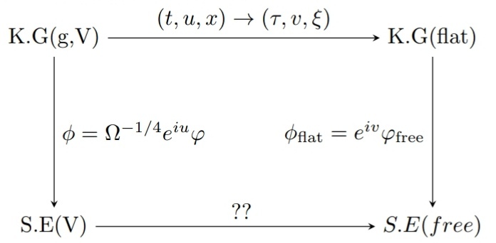
Figure 1: Schematic diagram showing how the transformation of the wave function is obtained.

Let us find explicitly the mapping between the wave functions. Using the covariance of the scalar field, $\phi(t,u,x)=\phi_{flat}(\tau,v,\xi)$ under the transformation $(t,u,x)\rightarrow(\tau,v,\xi)$, and the relation (41), we obtain $\Omega^{-1/4}e^{iu}\varphi_{V}=e^{iv}\varphi_{free}$ and, therefore,

$$\varphi_{V}(t,x)=\Omega^{1/4}e^{-i(u-v)}\varphi_{free}(\tau,\xi).$$ (43)

But $u-v=f_{3}$, and using (33) and (34), we get finally the wave function transformation

$$\varphi_{V}(t,x)=\Omega^{1/4}(t(\tau))e^{-if_{3}(\tau,\xi)}\,\varphi_{free}(\tau,\xi),$$ (44)

where

$$f_{3}(\tau,\xi)=\frac{\xi^{2}}{4\Omega(t(\tau))}\frac{d\Omega(t(\tau))}{d\tau}-\sqrt{\Omega(t(\tau))}\,\frac{dh}{d\tau}\,\xi$$

$$+\int{\left[\frac{\Omega(\tau)}{2}\left(\frac{dh(\tau)}{d\tau}\right)^{2}+\frac{S_{\tau}[\Phi(\tau)]h^{2}(\tau)}{4\Omega(\tau)}+\frac{B(\tau)h(\tau)+C(\tau)}{\Omega(\tau)}\right]}d\tau.\quad$$ (45)

This is the required mapping we were looking for. Here $\varphi_{V}(x,t)$ and $\varphi_{free}$ are solutions of the Schrodinger equation with potential $V(x,t)$ (under the constraint (29)) and with zero potential, respectively.

It is interesting to note that the transformation of the Eisenhart metric immediately gives us both the classical coordinate transformation and the quantum wave function transformation. The function $f_{3}$, as anticipated at the end of the previous section, appears as a phase in the transformation of the wave function.

In the following sections, we will explicitly find the most general maps between specific potentials and zero potential. In particular, we consider harmonic potential in section V and linear potential in section VI. We will deal with both time-independent and time-dependent cases and show that the previous results found in the literature are obtained as trivial sub-cases of our general results.

5 Harmonic oscillator to a free particle transformation

The relationship between quantum particles in zero and harmonic potentials appears to have been identified first in the field of optics [49, 50, 51]. The full mathematical equivalence of these problems was established by Niederer using group theoretical arguments [52]. In [53] Takagi explicitly showed how a quantum particle in harmonic potential can be mapped into a free particle. A fairly general result of this kind was also obtained by Arnold in the analysis of differential equations [3].

In this section, we show that these results are all special cases of a very general coordinate transformation. This will be done using the Eisenhart lift method as discussed in the previous sections. It is interesting to note that in the previous works of Takagi and Arnold, the mapping between a particle in harmonic potential and a free particle appears to be an ingenious guess. While in our case we are trying to classify all the potentials that will give us the flat Eisenhart metric, and by investigating this flatness condition, we find new transformations as a by-product and at the same time reproduce all the previous results already existing in the physical literature. In this respect, the Eisenhart lift method is more elegant.

As we have already mentioned, the most general potential compatible with the flatness condition is (36). This covers the cases of time-dependent and time-independent harmonic potentials and linear potential.

The time-dependent harmonic potential, $V(x,t)=\frac{1}{2}\omega^{2}(t)x^{2}$, corresponds to $B(t)=C(t)=0$ and

$$S_{t}(\Phi)=2\omega^{2}(t).$$ (46)

According to the general theory of Schwarzian derivative [56], (46) means that, $\Phi(t)=\frac{u_{1}(t)}{u_{2}(t)},$ where $u_{1}$ and $u_{2}$ are two linearly independent solutions of

$$\frac{d^{2}u(t)}{dt^{2}}+\omega^{2}(t)u(t)=0.$$ (47)

Then $\Omega(t)=\frac{d\Phi}{dt}=\frac{(u_{2}\frac{du_{1}}{dt}-u_{1}\frac{du_{2}}{dt})}{u_{2}^{2}}$. Let us choose the normalizations of $u_{1}$ and $u_{2}$ so that the Wronskian $W(u_{1},u_{2})=u_{2}\frac{du_{1}}{dt}-u_{1}\frac{du_{2}}{dt}=1$. In this case $\Omega(t)=\frac{1}{u_{2}^{2}(t)}$ and the equation for $h(\tau)$ takes the form

$$\frac{d^{2}h(\tau)}{d\tau^{2}}-\frac{2}{u_{2}(t(\tau))}\frac{du_{2}(t(\tau))}{d\tau}\,\frac{dh(\tau)}{d\tau}+\omega^{2}(t(\tau))u_{2}^{4}(t(\tau))h(\tau)=0.$$ (48)

For a given functional form of the frequency $\omega(t)$, we can solve (47) and find $u_{2}$, which in principle will allow us to solve (48) and find $h(\tau)$ and $p(\tau)$. Since $\tau=\int\Omega(t)dt=\Phi(t)$, from (31) and (33) we get the following coordinate transformations:

$$\tau=\frac{u_{1}(t)}{u_{2}(t)},\;\;\;\xi=\frac{x-h(\tau(t))}{u_{2}(t)},$$

$$v=u+\frac{[x-h(\tau(t))]^{2}}{2u_{2}(t)}\frac{du_{2}(t)}{dt}+\left[x-h(\tau(t))\right]\frac{dh(\tau(t))}{dt}-p(\tau(t)).\quad$$ (49)

Whereas, according to (44), the wave function is transformed as follows:

$$\varphi_{free}(\tau,\xi)=\sqrt{u_{2}(t)}\,e^{i\left[-\frac{[x-h(\tau(t))]^{2}}{2u_{2}(t)}\frac{du_{2}(t)}{dt}-\left[x-h(\tau(t))\right]\frac{dh(\tau(t))}{dt}+p(\tau(t))\right]}\varphi_{H.O}(t,x),$$ (50)

Equations (49) and (50) define the most general quantum transformation between a harmonic oscillator and a free particle. The trivial solution $h(\tau)=0$ of (48) corresponds to $\tau=\frac{u_{1}(t)}{u_{2}(t)}$, $\xi=\frac{x}{u_{2}(t)}$, which is exactly the Arnold transformation [3], and together with the transformation of the wave function

$$\varphi_{free}(\tau,\xi)=\sqrt{u_{2}(t)}\,e^{-i\left[\frac{x^{2}}{2u_{2}}\frac{du_{2}}{dt}\right]}\varphi_{H.O}(t,x)$$

they constitute the so-called ”Quantum Arnold transformation” [57].

In the case of a time-independent Harmonic potential, $\omega(t)=\omega_{0}$, two linearly independent solutions of (47) will be $u_{1}(t)=\frac{1}{\omega_{0}}sin(\omega_{0}t)$ and $u_{2}(t)=cos(\omega_{0}t)$. Our choice of $u_{2}$ is such that at $t=0$, $\Omega$ is well defined, and the normalization of $u_{1}$ is chosen in such a way as to make the Wronskian $W(u_{1},u_{2})=1$. Then $\Omega(t)=\frac{1}{u_{2}^{2}(t)}=\frac{1}{\cos^{2}{\omega_{0}t}}=\sec^{2}(\omega_{0}t)$ and $\tau=\frac{\tan(\omega_{0}t)}{\omega_{0}}$. In terms of $\tau$, we get $\Omega(\tau)=(1+\omega_{0}^{2}\tau^{2})$ and $u_{2}(\tau)=\frac{1}{\sqrt{1+\omega_{0}^{2}\tau^{2}}}$. Substituting $u_{2}(\tau)$ in (48), we get

$$\frac{d^{2}h(\tau)}{d\tau^{2}}+\frac{2\omega_{0}^{2}\tau}{1+\omega_{0}^{2}\tau^{2}}\,\frac{dh(\tau)}{d\tau}+\frac{\omega_{0}^{2}}{(1+\omega_{0}^{2}\tau^{2})^{2}}\,h(\tau)=$$

$$\frac{1}{\sqrt{1+\omega_{0}^{2}\tau^{2}}}\,\frac{d^{2}}{d\tau^{2}}\left[h(\tau)\,\sqrt{1+\omega_{0}^{2}\tau^{2}}\right]=0.$$ (51)

Therefore, the general form of the function $h(\tau)$ is

$$h(\tau)=\frac{c_{1}+c_{2}\,\omega_{0}\tau}{\sqrt{1+\omega_{0}^{2}\tau^{2}}},$$ (52)

where $c_{1}$ and $c_{2}$ arbitrary constants.

We can find $p(\tau)$ from (34):

$$p(\tau)=\int\left[-\frac{(1+\omega_{0}^{2}\tau^{2})}{2}\left(\frac{dh(\tau)}{d\tau}\right)^{2}+\frac{\omega_{0}^{2}h^{2}(\tau)}{2(1+\omega_{0}^{2}\tau^{2})}\right]d\tau=$$

$$\frac{(c_{1}^{2}-c_{2}^{2})\omega_{0}^{2}\tau-2c_{1}c_{2}\omega_{0}}{2(1+\omega_{0}^{2}\tau^{2})}+c_{3},$$ (53)

Where $c_{3}$ is an integration constant. Therefore, ultimately the transformation of coordinates takes the form

$$x=\frac{\xi+c_{2}\,\omega_{0}\tau+c_{1}}{\sqrt{1+\omega_{0}^{2}\tau^{2}}},\;\;\;t=f_{2}\left(\tau\right)=\frac{1}{\omega}\tan^{-1}\left(\omega\tau\right),\;\;\;u=v+f_{3}(\xi,\tau)=$$

$$v+\frac{\omega_{0}^{2}\xi^{2}\tau}{2(1+\omega_{0}^{2}\tau^{2})}-\frac{(c_{2}-c_{1}\,\omega_{0}\tau)\,\omega_{0}}{1+\omega_{0}^{2}\tau^{2}}\,\xi+\frac{(c_{1}^{2}-c_{2}^{2})\omega_{0}^{2}\tau-2c_{1}c_{2}\,\omega_{0}}{2(1+\omega_{0}^{2}\tau^{2})}+c_{3},\qquad$$ (54)

and the transformation law of the wave function becomes

$$\varphi_{H.O}(t,x)=(1+\omega_{0}^{2}\tau^{2})^{1/4}\times$$

$$e^{-i\left(\frac{\omega_{0}^{2}\xi^{2}\tau}{2(1+\omega_{0}^{2}\tau^{2})}-\frac{(c_{2}-c_{1}\omega_{0}\tau)\omega_{0}}{(1+\omega_{0}^{2}\tau^{2})}\xi+\frac{(c_{1}^{2}-c_{2}^{2})\omega_{0}^{2}\tau-2c_{1}c_{2}\omega_{0}}{2(1+\omega_{0}^{2}\tau^{2})}+c_{3}\right)}\varphi_{free}(\tau,\xi)$$ (55)

Equations (54) and (55) represent the most general and complete class of quantum transformations between a time-independent harmonic oscillator and free particle.

An important observation is that the transformations (55) are non-unitary due to the presence of the time dependent factor $(1+\omega_{0}^{2}\tau^{2})^{1/4}$. Thus, these transformations cannot represent the principle of equivalence, in contrast to the case of linear potential (gravity), considered below. It is impossible to reconstruct the entire temporal history of a harmonic oscillator from the temporal history of a free particle using only one transformation (54) (or (49) in the case of time-dependent oscillator). This situation is analogous to the situation in geometry then a manifold cannot be covered by a single patch of coordinates [53].

In the limiting case $c_{1}=0=c_{2}$, which implies $h(\tau)=0$ and $p(\tau)=0$, one recovers the solution already known in the literature as the Niederer transformation [52, 58, 59]. In fact, all the previous results relating one-dimensional harmonic potential to zero potential are special cases of the most general transformation (49).

6 Mapping a linear potential to a free particle

Having considered in detail the case of a harmonic oscillator in the previous section, we now consider the case of a linear potential. A linear potential $V=g(t)\,x$ can be associated with a weak gravitational field. A beautiful neutron interference experiment [61] revealed quantum effects in such fields. Mathematically, these quantum effects arise from the phase transformation of the wave function caused by the transformation of coordinates in the Schrödinger equation during the transition from an inertial coordinate system to an accelerated one [62]. The same effect was observed when setting the entire neutron interferometer into harmonic oscillations and measuring the phase shift as a function of the apparatus maximal acceleration, which demonstrates the validity of the equivalence principle in the nonrelativistic quantum regime [63]. Sakurai’s book [64] contains a brief pedagogical account of neutron interference phenomena in the presence of a weak gravitational potential.

In this section, we will discuss the equivalence between a linear potential and a free particle using the Eisenhart lift and find out explicitly the most general coordinate transformations together with the corresponding quantum phase transformations. It is shown that the transformation representing the equivalence principle is a special case of these general transformations. We report a new class of non-unitary transformations previously unknown to the authors. We consider both time-independent and time-dependent cases.

Time-dependent linear potential, $V(x,t)=B(t)\,x$, corresponds to $C(t)=0$ and $S_{t}(\Phi)=0$ in (36). From the theory of the Schwarzian derivative, we know that the general solution of the equation $S_{t}(\Phi)=0$ is given by the Möbius transformation $\Phi(t)=\frac{at+b}{ct+d}$, $k=ad-bc\neq 0$. First consider the case $c\neq 0$. Then $\Phi(t)=\frac{a}{c}-\frac{k}{c(ct+d)}$, and $\Omega(t)=\frac{d\Phi}{dt}=\frac{k}{(ct+d)^{2}}$, $\tau=\int\Omega(t)dt=\frac{-k}{c(ct+d)}$. Therefore, $\Omega(\tau)=\frac{c^{2}\tau^{2}}{k}$. If we substitute this into (35), we get

$$\frac{d^{2}h(\tau)}{d\tau^{2}}+\frac{2}{\tau}\frac{dh(\tau)}{d\tau}=\frac{1}{\tau^{2}}\,\frac{d}{d\tau}\left(\tau^{2}\,\frac{dh(\tau)}{d\tau}\right)=-\frac{B(t(\tau))\,k^{2}}{c^{4}\tau^{4}}.$$ (56)

The general solution of this differential equation is

$$h(\tau)=-\frac{k^{2}}{c^{4}}\int\frac{1}{\tau^{2}}\left[\int\frac{B(t(\tau))}{\tau^{2}}d\tau\right]d\tau-\frac{c_{1}}{\tau}+c_{2},$$ (57)

where $c_{1}$, $c_{2}$ are arbitrary constants. Then $p(\tau)$ is determined from (34):

$$p(\tau)=\int\left[\frac{-c^{2}\tau^{2}}{2k}\left(-\frac{k^{2}}{c^{4}\tau^{2}}\int\frac{B(t(\tau))}{\tau^{2}}d\tau+\frac{c_{1}}{\tau^{2}}\right)^{2}+\right.$$

$$\left.\frac{B(t(\tau))k}{c^{2}\tau^{2}}\left(-\frac{k^{2}}{c^{4}}\int\frac{1}{\tau^{2}}\left[\int\frac{B(t(\tau))}{\tau^{2}}d\tau\right]d\tau-\frac{c_{1}}{\tau}+c_{2}\right)\right]d\tau.$$ (58)

Correspondingly, according to (33), the coordinate transformation becomes

$$t=\frac{-k}{c^{2}\tau}-\frac{d}{c},\;\;\;x=\frac{\sqrt{k}\,\xi}{c\tau}-\frac{k^{2}}{c^{4}}\int\frac{1}{\tau^{2}}\left[\int\frac{B(t(\tau))}{\tau^{2}}d\tau\right]d\tau-\frac{c_{1}}{\tau}+c_{2},$$ (59)

$$f_{3}=\frac{\xi^{2}}{2\tau}-\frac{c\tau\,\xi}{\sqrt{k}}\left(-\frac{k^{2}}{c^{4}\tau^{2}}\int\frac{B(t(\tau))}{\tau^{2}}d\tau+\frac{c_{1}}{\tau^{2}}\right)+p(\tau),$$

and the wave function transforms as

$$\varphi_{grv}(t,x)=\frac{\sqrt{c\,\tau}}{k^{1/4}}\,e^{-i\left[\frac{\xi^{2}}{2\tau}-\frac{c\tau\xi}{\sqrt{k}}\left(-\frac{k^{2}}{c^{4}\tau^{2}}\int\frac{B(t(\tau))}{\tau^{2}}d\tau+\frac{c_{1}}{\tau^{2}}\right)+p(\tau)\right]}\varphi_{free}(\tau,\xi),$$ (60)

where $p(\tau)$ is given by (58).

Thus, we have found the desired transformation, and it turned out to be non-unitary. Interestingly, it appears that this result was not previously known. We believe that no one has ever looked for the aforementioned transformation that connects a linear potential and a free particle due to the limited use of non-unitary transformations.

For transparency and comparison with previous results, these transformations can be simplified by setting $B(t)=g=\mathrm{const}$, $k=1$, $c=1/\tau_{0}$, $d=0$, $c_{1}=0$ and $c_{2}=0$ ($\tau_{0}$ is some constant with the dimension of time). As a result, we get

$$t=-\frac{\tau_{0}^{2}}{\tau},\;\;\;x=\frac{\xi\tau_{0}}{\tau}-\frac{g\tau_{0}^{4}}{2\tau^{2}},\;\;\;f_{3}=\frac{\xi^{2}}{2\tau}-\frac{g\xi\tau_{0}^{3}}{\tau^{2}}+\frac{g^{2}\tau_{0}^{6}}{3\tau^{3}},$$ (61)

$$\varphi_{grv}(t,x)=\sqrt{\frac{\tau}{\tau_{0}}}\,e^{-i\left[\frac{\xi^{2}}{2\tau}-\frac{g\xi\tau_{0}^{3}}{\tau^{2}}+\frac{g^{2}\tau_{0}^{6}}{3\tau^{3}}\right]}\varphi_{free}(\tau,\xi).$$

This transformation, in its simplest form, is a new equivalence between the time-independent linear potential and the case of free particles.

Now consider the case $c=0$. Then $\Omega=\frac{a}{d}=\mathrm{const}$ and without loss of generality we can assume $\Omega=1$. In this case, the equation for $h(\tau)$ according to (35) becomes

$$\frac{d^{2}h(\tau)}{d\tau^{2}}=-B(t(\tau)),$$ (62)

with a solution (for simplicity, we dropped the integration constants)

$$h(\tau)=-\int d\tau\int B(t(\tau))\,d\tau.$$ (63)

Correspondingly, (34) will gives us $p(\tau)$:

$$p(\tau)=\int\left[-\frac{1}{2}\left(\int B(t(\tau))d\tau\right)^{2}-B(t(\tau))\int d\tau\int B(t(\tau))\,d\tau\right]d\tau,$$ (64)

and we get the following transformation of coordinates, along with the corresponding wave function transformation:

$$\tau=t,\;\;\;x=\xi-\int d\tau\int B(t(\tau))\,d\tau,\;\;\;f_{3}\left(\xi,\tau\right)=\xi\int B(t(\tau))\,d\tau+p(\tau),$$

$$\varphi_{grv}(t,x)=e^{-i\left[\xi\int B(t(\tau))\,d\tau+p\left(\tau\right)\right]}\varphi_{free}(\tau,\xi).$$ (65)

Using integration by parts, we can transform the second term in (64) as follows

$$\int-B(t(\tau))\left[\int d\tau\int B(t(\tau))\,d\tau\right]d\tau=\int B(t(\tau))h(\tau)\,d\tau=$$

$$-\int\frac{d^{2}h(\tau)}{d\tau^{2}}h(\tau)\,d\tau=-h(\tau)\frac{dh(\tau)}{d\tau}+\int\left(\frac{dh(\tau)}{d\tau}\right)^{2}d\tau.$$

Therefore,

$$p(\tau)=\frac{1}{2}\int\left(\frac{dh(\tau)}{d\tau}\right)^{2}d\tau-h(\tau)\frac{dh(\tau)}{d\tau},$$

and we get

$$f_{3}\left(\xi,\tau\right)=-\left(\xi+h(\tau)\right)\frac{dh(\tau)}{d\tau}+\frac{1}{2}\int\left(\frac{dh(\tau)}{d\tau}\right)^{2}d\tau,$$

$$\varphi_{grv}(t,x)=e^{i\left[\left(\xi+h(\tau)\right)\frac{dh(\tau)}{d\tau}-\frac{1}{2}\int\left(\frac{dh(\tau)}{d\tau}\right)^{2}d\tau\right]}\varphi_{free}(\tau,\xi),$$ (66)

where $h(\tau)$ is a solution of (61). This is exactly the transformation that was presented in [65] as an implementation of the well-known weak equivalence principle for the time-dependent gravitational field. It becomes much more recognizable when $B(t)=g$ is a constant. Then the transformation takes the form

$$t=\tau,\;\;\;x=\xi-\frac{g\tau^{2}}{2},\;\;u=v+f_{3}=v+g\xi\tau-\frac{g^{2}\tau^{3}}{3},$$

$$\varphi_{grv}(t,x)=e^{-i\left[g\xi\tau-\dfrac{g^{2}\tau^{3}}{3}\right]}\varphi_{free}(\tau,\xi).$$ (67)

This transformation is known to be a quantum formulation of Einstein’s principle of equivalence in the context of nonrelativistic quantum mechanics [66].

7 Conclusions

In this note, we discussed the relationship between the wave functions of a harmonic oscillator and a free particle using the Eisenhart lift method. We show that only two types of potentials, namely quadratic and linear can be mapped to the zero potential case. This somewhat surprising result has simple geometric interpretation: the corresponding Eisenhart manifolds are flat.

Only one-dimensional dynamical systems and their Eisenhart lifts have been considered. However, the beautiful result that the linearizability criteria are equivalent to the requirement that the underlying manifold be flat is true in the much broader context of ordinary differential equations that can be projected from a system of geodesic equations [67, 68].

In this article, we did not consider the possibility of non-trivial values of $g(x,t)$ in (11), which will further expand the possibilities of including other potentials, such as the Morse potential, damped harmonic oscillator, etc. Research in this direction has the potential to be very interesting.

In conclusion, the study of nonrelativistic physics through the prism of higher-dimensional relativistic theories opens up many opportunities for further understanding of various aspects of nonrelativistic phenomena and can be useful, for example, in nonrelativistic holography [46, 69], which has been gaining attention lately. The Eisenhart Lift Method seems to be a useful tool in this regard, and we hope to conduct further research in this direction.

References

- [1] S.-S. Chern, From Triangles to Manifolds, Amer. Math. Monthly 86 (1979), 339–349. https://doi.org/10.2307/2321093
- [2] A. Weinstein, Symplectic geometry, Bull. Amer. Math. Soc. 5 (1981), 1–13. https://doi.org/10.1090/S0273-0979-1981-14911-9
- [3] V. I. Arnold, Mathematical Methods of Classical Mechanics (Springer: New York, 1989). https://doi.org/10.1007/978-1-4757-2063-1
- [4] H. Geiges, A Brief History of Contact Geometry and Topology, Expo. Math. 19 (2001), 25–53. https://doi.org/10.1016/S0723-0869(01)80014-1
- [5] P. Ševera, Contact geometry in Lagrangean mechanics, J. Geom. Phys. 29 (1999), 235–242. https://doi.org/10.1016/S0393-0440(98)00037-0
- [6] G. B. Halsted, Biography: Paenutij Lvovitsch Tchebychev, Am. Math. Monthly 2N3 (1895), 61–63. https://doi.org/10.2307/2969930
- [7] K. Morand, Embedding Galilean and Carrollian geometries I. Gravitational waves, J. Math. Phys. 61 (2020), 082502. https://doi.org/10.1063/1.5130907
- [8] M. Atiyah, Einstein and Geometry, Curr. Sci. 89 (2005), 2041–2044. https://doi.org/10.1142/9789812772718_0002
- [9] A. McInerney, First Steps in Differential Geometry: Riemannian, Contact, Symplectic (Springer: New York, 2013). https://doi.org/10.1007/978-1-4614-7732-7
- [10] P. Bargueño, Nonrelativistic gauged quantum mechanics: From Kaluza-Klein compactifications to Bargmann structures, Phys. Lett. A 379 (2015), 1563-1567. https://doi.org/10.1016/j.physleta.2015.02.047
- [11] X. Bekaert and K. Morand, Embedding nonrelativistic physics inside a gravitational wave, Phys. Rev. D 88 (2013), 063008. https://doi.org/10.1103/PhysRevD.88.063008
- [12] C. Duval, G. Burdet, H. P. Künzle and M. Perrin, Bargmann Structures and Newton-cartan Theory, Phys. Rev. D 31 (1985), 1841–1853. https://doi.org/10.1103/PhysRevD.31.1841
- [13] L. P. Eisenhart, Dynamical trajectories and geodesics, Annals. Math. 30 (1928-1929) 591–606. https://doi.org/10.2307/1968307
- [14] M. W. Brinkmann, On Riemann spaces conformal to Euclidean space, Proc. Natl. Acad. Sci. U.S. 9 (1923) 1–3. https://doi.org/10.1073/pnas.9.1.1
- [15] M. W. Brinkmann, Einstein spaces which are mapped conformally on each other, Math. Ann. 94 (1925) 119–145. https://doi.org/10.1007/BF01208647
- [16] M. Cariglia, C. Duval, G. W. Gibbons and P. A. Horvathy, Eisenhart lifts and symmetries of time-dependent systems, Annals Phys. 373 (2016) 631–654. https://doi.org/10.1016/j.aop.2016.07.033
- [17] M. Cariglia, Hidden symmetries of Eisenhart-Duval lift metrics and the Dirac equation with flux, Phys. Rev. D 86 (2012), 084050. https://doi.org/10.1103/PhysRevD.86.084050
- [18] G. W. Gibbons and C. N. Pope, Kohn’s Theorem, Larmor’s Equivalence Principle and the Newton-Hooke Group, Annals Phys. 326 (2011), 1760-1774. https://doi.org/10.1016/j.aop.2011.03.003
- [19] K. Finn, S. Karamitsos and A. Pilaftsis, Quantizing the Eisenhart Lift, Phys. Rev. D 103 (2021), 065004. https://doi.org/10.1103/PhysRevD.103.065004
- [20] K. Finn, S. Karamitsos and A. Pilaftsis, Eisenhart lift for field theories, Phys. Rev. D 98 (2018), 016015. https://doi.org/10.1103/PhysRevD.98.016015
- [21] C. Duval, M. Hassaine and P. A. Horvathy, The Geometry of Schrödinger symmetry in gravity background/non-relativistic CFT, Annals Phys. 324 (2009), 1158-1167. https://doi.org/10.1016/j.aop.2009.01.006
- [22] C. Duval and S. Lazzarini, Schrödinger Manifolds, J. Phys. A 45 (2012), 395203. https://doi.org/10.1088/1751-8113/45/39/395203
- [23] N. Kan, T. Aoyama, T. Hasegawa and K. Shiraishi, Eisenhart lift for minisuperspace quantum cosmology, arXiv:2105.09514 [gr-qc]. https://arxiv.org/abs/2105.09514
- [24] M. Cariglia, A. Galajinsky, G. W. Gibbons and P. A. Horvathy, Cosmological aspects of the Eisenhart-Duval lift, Eur. Phys. J. C 78 (2018), 314. https://doi.org/10.1140/epjc/s10052-018-5789-x
- [25] E. Minguzzi, Eisenhart’s theorem and the causal simplicity of Eisenhart’s spacetime, Class. Quant. Grav. 24 (2007), 2781–2808. https://doi.org/10.1088/0264-9381/24/11/002
- [26] M. Cariglia and F. K. Alves, The Eisenhart lift: a didactical introduction of modern geometrical concepts from Hamiltonian dynamics, Eur. J. Phys. 36 (2015), 025018. https://doi.org/10.1088/0143-0807/36/2/025018
- [27] E. Minguzzi, Classical aspects of lightlike dimensional reduction, Class. Quant. Grav. 23 (2006), 7085–7110. https://doi.org/10.1088/0264-9381/23/23/029
- [28] C. W. Misner, K. S. Thorne and J. A. Wheeler, Gravitation (Princeton University Press: Princeton, 2017).
- [29] K. F. Sundman, Mémoire sur le problém des trois corps, Acta Math. 36 (1912-1913), 105–179. https://doi.org/10.1007/BF02422379
- [30] P. Guha, B. Khanra and A. G. Choudhury, On generalized Sundman transformation method, first integrals, symmetries and solutions of equations of Painlevé-Gambier type, Nonlinear Anal. 72 (2010), 3247–3257. https://doi.org/10.1016/j.na.2009.12.004
- [31] J. Barrow-Green, The dramatic episode of Sundman, Historia Mathematica 37 (2010), 164–203. https://doi.org/10.1016/j.hm.2009.12.004
- [32] A. Lichnerowicz, Théories Relativistes de la Gravitation et de l’Électromagnetisme (Masson: Paris, 1955).
- [33] L. P. Eisenhart, Riemannian Geometry (Princeton University Press: Princeton, 1997).
- [34] A. Garcia, F. W. Hehl, C. Heinicke and A. Macias, The Cotton tensor in Riemannian space-times, Class. Quant. Grav. 21 (2004), 1099–1118. https://doi.org/10.1088/0264-9381/21/4/024
- [35] C. Duval, P. A. Horvathy and L. Palla, Conformal Properties of Chern-Simons Vortices in External Fields, Phys. Rev. D 50 (1994), 6658–6661. https://doi.org/10.1103/PhysRevD.50.6658
- [36] C. Duval, G. W. Gibbons and P. Horvathy, Celestial mechanics, conformal structures and gravitational waves, Phys. Rev. D 43 (1991), 3907–3922. https://doi.org/10.1103/PhysRevD.43.3907
- [37] C. Duval, Z. Horvath and P. A. Horvathy, Vanishing of the conformal anomaly for strings in a gravitational wave, Phys. Lett. B 313 (1993), 10–14. https://doi.org/10.1016/0370-2693(93)91183-N
- [38] P. Horvathy, private communication.
- [39] D. McMahon, Relativity Demystified (McGraw-Hill: New York, 2006). http://mhebooklibrary.com/doi/book/10.1036/0071455450
- [40] M. Gasperini, Theory of Gravitational Interactions (Springer-Verlag: Berlin, 2013). https://doi.org/10.1007/978-3-319-49682-5
- [41] D. F. Carneiro, E. A. Freiras, B. Goncalves, A. G. de Lima and I. L. Shapiro, On useful conformal tranformations in general relativity, Grav. Cosmol. 10 (2004), 305–312. https://arxiv.org/abs/gr-qc/0412113
- [42] V. Faraoni, E. Gunzig and P. Nardone, Conformal transformations in classical gravitational theories and in cosmology, Fund. Cosmic Phys. 20 (1999), 121. https://arxiv.org/abs/gr-qc/9811047
- [43] V. Ovsienko and S. Tabachnikov, What is .. the Schwarzian derivative? Notices Am. Math. Soc. 56(1) (2009), 34–36. https://www.ams.org/notices/200901/tx090100034p.pdf
- [44] O. Lehto, Univalent Functions and Teichmüller Spaces (Springer: New York, 1987). https://doi.org/10.1007/978-1-4613-8652-0
- [45] B. Osgood, Old and New on the Schwarzian Derivative, in P. Duren, J. Heinonen, B. Osgood and B. Palka (Eds.), Quasiconformal Mappings and Analysis (Springer: New York, 1998). https://doi.org/10.1007/978-1-4612-0605-7_16
- [46] F. L. Lin and S. Y. Wu, Non-relativistic Holography and Singular Black Hole, Phys. Lett. B 679 (2009), 65–72. https://doi.org/10.1016/j.physletb.2009.07.002
- [47] R. Penrose, A Remarkable property of plane waves in general relativity, Rev. Mod. Phys. 37 (1965), 215–220. https://doi.org/10.1103/RevModPhys.37.215
- [48] M. Blau, M. Borunda, M. O’Loughlin and G. Papadopoulos, Penrose limits and space-time singularities, Class. Quant. Grav. 21 (2004), L43–L49. https://doi.org/10.1088/0264-9381/21/7/L02
- [49] A. Yariv, Quantum Electronics (Wiley: New York, 1967).
- [50] O. Steuernagel, Equivalence between free quantum particles and those in harmonic potentials and its application to instantaneous changes, Eur. Phys. J. Plus 129 (2014), 114. https://doi.org/10.1140/epjp/i2014-14114-3
- [51] O. Steuernagel, Equivalence between focused paraxial beams and the quantum harmonic oscillator, Am. J. Phys. 73 (2005), 625–629. https://doi.org/10.1119/1.1900099
- [52] U. Niederer, The maximal kinematical invariance group of the harmonic oscillator, Helv. Phys. Acta 46 (1973), 191–200. https://doi.org/10.5169/seals-114478
- [53] S. Takagi, Equivalence of a Harmonic Oscillator to a Free Particle, Prog. Theor. Phys. 84 (1990), 1019–1024. https://doi.org/10.1143/ptp/84.6.1019
- [54] M. Oliva, D. Kakofengitis and O. Steuernagel, Anharmonic quantum mechanical systems do not feature phase space trajectories, Physica A 502 (2018) 201–210. https://doi.org/10.1016/j.physa.2017.10.047
- [55] D. Kakofengitis, M. Oliva and O. Steuernagel, Wigner’s representation of quantum mechanics in integral form and its applications, Phys. Rev. A 95 (2017), 022127. https://doi.org/10.1103/PhysRevA.95.022127
- [56] R. L. Devaney and L. Keen, Dynamics of meromorphic maps with polynomial Schwarzian derivative, Ann. Sci. École Norm. Sup. 22 (1989), 55–81.
- [57] V. Aldaya, F. Cossío, J. Guerrero and F. F. López-Ruiz, The quantum Arnold transformation, J. Phys. A: Math. Theor. 44 (2011), 065302. https://doi.org/10.1088/1751-8113/44/6/065302
- [58] O. Steuernagel, Equivalence between free quantum particles and those in harmonic potentials and its application to instantaneous changes, Eur. Phys. J. Plus 129 (2014), 114. https://doi.org/10.1140/epjp/i2014-14114-3
- [59] K. Andrzejewski and S. Prencel, Niederer’s transformation, time-dependent oscillators and polarized gravitational waves, Clas. Quantun Grav. 36 (2019), 155008. https://doi.org/10.1088/1361-6382/ab2394
- [60] Q. L. Zhao, P. M. Zhang and P. A. Horvathy, Time-dependent conformal transformations and the propagator for quadratic systems, arXiv:2105.07374 [quant-ph]. https://arxiv.org/abs/2105.07374
- [61] R. Colella and A. W. Overhauser, How the COW happened, Physica B 385-386 (2006), 1408-1410. https://doi.org/10.1016/j.physb.2006.05.200
- [62] R. Colella, A. W. Overhauser and S. A. Werner, Observation of gravitationally induced quantum interference, Phys. Rev. Lett. 34 (1975), 1472-1474. https://doi.org/10.1103/PhysRevLett.34.1472
- [63] U. Bonse and T. Wroblewski, Measurement of Neutron Quantum Interference in Noninertial Frames, Phys. Rev. Lett. 51 (1983), 1401-1404. https://doi.org/10.1103/physrevlett.51.1401
- [64] J. J. Sakurai, Modern Quantum Mechanics (Addison-Wesley: Reading, 1994).
- [65] D. Giulini, Equivalence principle, quantum mechanics, and atom-interferometric tests. In F. Finster et al. (editors), Quantum Field Theory and Gravity, (Springer Verlag: Basel, 2012), pp. 345-370. https://arxiv.org/abs/1105.0749
- [66] M. Nauenberg, Einstein’s equivalence principle in quantum mechanics revisited, Am. J. Phys. 84 (2016), 879-882. https://doi.org/10.1119/1.4962981
- [67] A. V. Aminova and N. A.-M. Aminov, Projective geometry of systems of second-order differential equations, Sb. Math. 197 (2006), 951-975. https://doi.org/10.1070/SM2006v197n07ABEH003784
- [68] A. Qadir, Linearization: Geometric, Complex, and Conditional, J. Appl. Math., vol. 2012 (2012), 303960. https://doi.org/10.1155/2012/303960
- [69] M. Cariglia, General theory of Galilean gravity, Phys. Rev. D 98 (2018), 084057. https://doi.org/10.1103/PhysRevD.98.084057