A Neutron Star is born

Abstract

A neutron star was first detected as a pulsar in 1967. It is one of the most mysterious compact objects in the universe, with a radius of the order of 10 km and masses that can reach two solar masses. In fact, neutron stars are star remnants, a kind of stellar zombies (they die, but do not disappear). In the last decades, astronomical observations yielded various contraints for the neutron star masses and finally, in 2017, a gravitational wave was detected (GW170817). Its source was identified as the merger of two neutron stars coming from NGC 4993, a galaxy 140 million light years away from us. The very same event was detected in $\gamma$-ray, x-ray, UV, IR, radio frequency and even in the optical region of the electromagnetic spectrum, starting the new era of multi-messenger astronomy. To understand and describe neutron stars, an appropriate equation of state that satisfies bulk nuclear matter properties is necessary. GW170817 detection contributed with extra constraints to determine it. On the other hand, magnetars are the same sort of compact objects, but bearing much stronger magnetic fields that can reach up to 10¹⁵ G on the surface as compared with the usual 10¹² G present in ordinary pulsars. While the description of ordinary pulsars is not completely established, describing magnetars poses extra challenges. In this paper, I give an overview on the history of neutron stars and on the development of nuclear models and show how the description of the tiny world of the nuclear physics can help the understanding of the cosmos, especially of the neutron stars.

I Introduction

Two of the known existing interactions that determine all the conditions of our Universe are of nuclear origin: the strong and the weak nuclear forces. It is not possible to talk about neutron stars without understanding them, and specially the strong nuclear interaction, which is well described by the Quantum Chromodynamics (QCD). But notice: a good description through a Lagrangian density does not mean that the solutions are known for all possible systems subject to the strong nuclear force.

Based on the discovery of asymptotic freedom asym , which predicts that strongly interacting matter undergoes a phase transition from hadrons to the quark-gluon plasma (QGP) and on the possibility that a QGP could be formed in heavy-ion collisions, the QCD phase diagram has been slowly depicted. While asymptotic freedom is expected to take place at both high temperatures, as in the early universe and high densities, as in neutron star interiors, heavy-ion collisions can be experimentally tested with different energies at still relatively low densities, but generally quite high temperatures. If one examines the QCD phase diagram, shown in Fig. 1, it is possible to see that the nuclei occupy a small part of the diagram, at low densities and low temperatures for different asymmetries. One should notice the temperature log scale, chosen to emphasise the region where nuclei exist. Neutron stars, on the other hand, are compact objects with a density that can reach 10 times the nuclear saturation density, discussed later on along this paper. While heavy ion collisions probe experimentally some regions of the diagram, lattice QCD (LQCD) calculations explain only the low density region close to zero baryonic chemical potential. Hence, we rely on effective models to advance our understanding and they are the main subject of this paper.

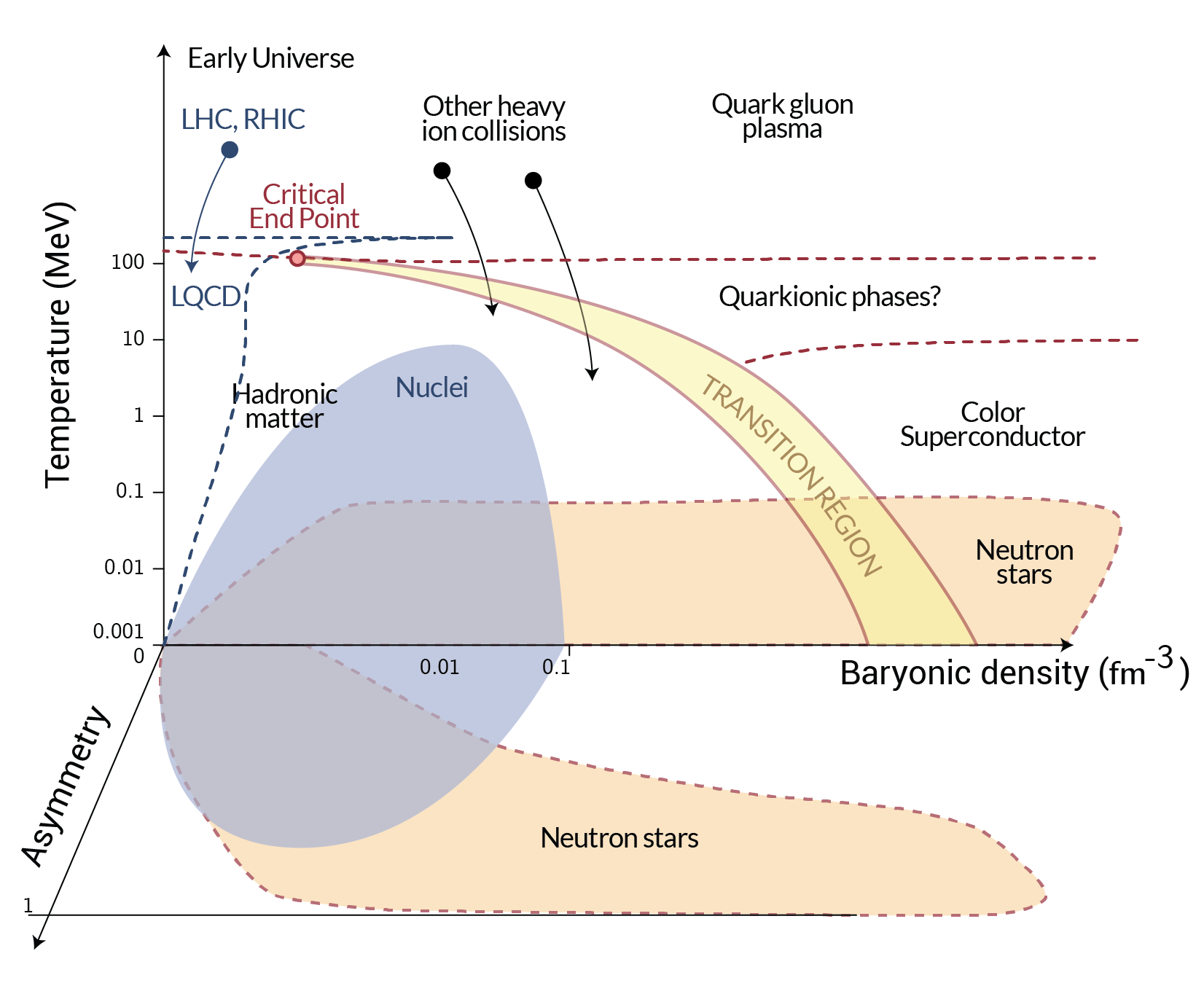
Figure 1: QCD phase diagram. On the left of the transition region stands hadronic matter and on the right side, the quark gluon plasma. Quarkyonic phases represent a region where chiral symmetry has been restored but matter is still confined. Figure taken and adapted from annawatts .

Since the beginning of the last century, many nuclear models have been proposed. In Section II.1, the first models are mentioned and the notion of nuclear matter discussed. The formalisms that followed, either non-relativistic Skyrme-type models skyrme or relativistic ones that gave rise to the quantum hadrodynamics model were based on some basic features described by the early models, the liquid drop model liquiddrop and the semi-empirical mass formula semiempirical . Once the nuclear physics is established, the very idea of a neutron star can be tackled. However, it is very important to have in mind the model extrapolations that may be necessary when one moves from the nuclei region shown in Fig. 1 to the neutron star (NS) region. A simple treatment of the relation between these two regions and the construction of the QCD phase transition line can be seen in Carline2 .

The exact constitution of these compact objects, also commonly named pulsars due to their precise rotation period, is still unknown and all the information we have depends on the confrontation of theory with astrophysical observations. As the density increases towards their center, it is believed that there is an outer crust, an inner crust, an outer core and an inner core. The inner core constitution is the most controversial: it can be matter composed of deconfined quarks or perhaps a mixed phase of hadrons and quarks. I will try to comment and describe every one of the possible layers inside a NS along this text.

NASA’s Neutron Star Interior Composition Explorer (NICER), an x-ray telescope NICER launched in 2017, has already sent some news NICER_news : by monitoring the x-ray emission of gas surrounding the heaviest known pulsar, PSR J0740+6620 with a mass of $2.08\pm 0.07$, it has measured its size and it is larger than previously expected, a diameter of around 25 to 27 km, with consequences on the possible composition of the NS core.

In this paper, I present a comprehensive review of the main nuclear physics properties that should be satisfied by equations of states aimed to describe nuclear matter, the consequences arising from the extrapolation necessary to describe objects with much higher densities as neutron stars and how they can be tuned according to observational constraints. At the end, a short discussion on quark and hybrid stars is presented and the existence of magnetars is rapidly outlined. Not all important aspects related to neutron stars are treated in the present work, rotation being the most important one that is disregarded, but the interested reader can certainly use it as an initiation to the physics of these compact objects.

II Historical perspectives

I divide this section, which concentrates all necessary information for the development of the physics of neutron stars, in two parts. In the first one, I discuss the development of the nuclear physics models based on known experimental properties and introduce the very simple Fermi gas model, whose calculation is later used in more realistic relativistic models. The second part is devoted to the history of compact objects from the astrophysical point of view.

II.1 From the nuclear physics point of view

The history of nuclear physics modelling started with two very simple models: the liquid drop model, introduced in 1929 liquiddrop and the semi-empirical mass formula, proposed in 1935 by Bethe and Weizsäcker semiempirical .

The liquid drop model idea came from the observation that the nucleus has behavior and properties that resemble the ones of an incompressible fluid, such as: a) the nucleus has low compressibility due to its internal almost constant density; b) it presents well defined surface; c) the nucleus radius varies with the number of nucleons as $R=R_{0}A^{1/3}$, where $R_{0}\simeq 1.2\times 10^{-15}$ m and d) the nuclear force is isospin independent and saturates.

Typical nuclear density profiles are shown in Fig. 2, from where one can observe some of the features mentioned above, i.e., the density is almost constant up to a certain point and then it drops rapidly close to the surface, determining the nucleus radius. The mean square radius is usually defined as

$$R_{i}^{2}=\frac{\int d^{3}r\,r^{2}\rho_{i}(\mathbf{r})}{\int d^{3}r\,\rho_{i}(\mathbf{r})},\quad i=p,n$$ (1)

where $\rho_{p}$ is the number density of protons and $\rho_{n}$ the number density of neutrons.

A nucleus with an equal number of protons and neutrons has a slightly larger proton radius because they repel each other due to the Coulomb interaction. A nucleus with more neutrons than protons (as most of the stable ones) has a larger neutron radius than its proton counterpart and the small difference between both radii is known as neutron skin thickness, given by skin ; skin2 ; PREX1 ; PREX2 :

$$\theta=R_{n}-R_{p}.$$ (2)

For the last two decades, a precise measurement of both charge and neutron radii of the ²⁰⁸Pb nucleus has been tried at the parity radius experiment (PREX) at the Jefferson National Accelerator Facility Jefflab using polarised electron scattering. The latest experimental results PREX2 point to $\theta=0.283\pm 0.071$ fm and to the interior baryon density $\rho_{0}=0.1480\pm 0.0036({\rm exp})\pm 0.0013({\rm theo})$ fm^-3. These quantities have shown to be important for the understanding of some of the properties of the neutron star. I will go back to this discussion later on.

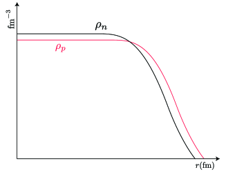
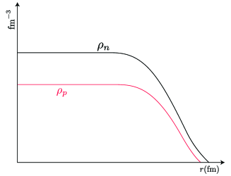
Figure 2: Schematic representation of the nuclear densities with equal number of protons and neutrons (top) and a larger number of neutrons than protons (bottom). The proton and neutron densities depend on the number of nucleons so that heavier elements present larger densities. Typical theoretical densities for ²⁰⁸Pb are of the order of 0.09 fm^-3 for neutrons and 0.06 - 0.07 fm^-3 for protons skin2 .

The binding energy $B$ of a nucleus ${}^{A}_{Z}X_{N}$ is given by the difference between its mass and the mass of its constituents ($Z$ protons and $N$ neutrons):

$$B=(Zm_{p}+Nm_{n}-(m(^{A}_{Z}X)-Zm_{e}))c^{2}$$

$$=(Zm(^{1}H)+Nm_{n}-m(^{A}_{Z}X))c^{2},$$ (3)

where $m(^{A}_{Z}X)$ is the mass of the chemical element ${}^{A}_{Z}X$ and is given in atomic mass units. The binding energy per nucleon $\frac{B}{A}$ is shown in Fig. 3, from where it is seen that the curve is relatively constant and of the order of $8.5$ MeV except for light nuclei. The semi-empirical mass formula, which is a parameter dependent expression was used to fit the experimental results successfully and it reads:

$$B(Z,A)=a_{v}A-a_{s}A^{\frac{2}{3}}-a_{c}e^{2}\frac{Z(Z-1)}{A^{\frac{1}{3}}}-a_{i}\frac{(N-Z)^{2}}{A}+\delta(A).$$ (4)

In this equation, from left to right, the quantities refer to a volume term, a surface term, a Coulomb term, an energy symmetry term and a pairing interaction term livro2 ,livro1 . Of course, with so many parameters, other parameterisations can be obtained from the fitting of the data. One possible set is $a_{v}=15.68$ MeV, $a_{s}=18.56$ MeV, $a_{c}\times e^{2}=0.72$ MeV, $a_{i}=18.1$ MeV and

$$\delta=\begin{cases}34~{}~{}A^{-3/4}{\rm MeV},&{\rm even-even~{}nuclei},\cr 0,&{\rm even-odd~{}nuclei},\cr-34~{}~{}A^{-3/4}{\rm MeV},&{\rm odd-odd~{}nuclei}.\cr\end{cases}$$ (5)

Figure 3: Binding energy per nucleon as a function of the number of nucleons.

Although quite naive, these two models combined can explain many important nuclear physics properties, as nuclear fission, for instance livro1 .

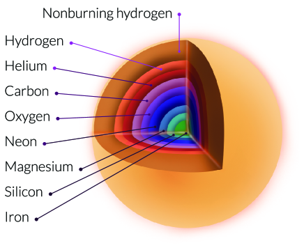
Figure 4: Naive schematic representation of the possible chemical elements synthesised in stellar fusion. Heavier elements are produced in dense stellar matter. Notice that these elements are produced in normal stars, not neutron stars.

Parameter dependent nuclear models can also explain the fusion of the elements in the stars and the primordial nucleosynthesis with the abundance of chemical elements in the observable universe, which is roughly the following: 71% is Hydrogen, 27% is Helium, 1.8% are Carbon to Neon elements, 0.2% are Neon to Titanium, 0.02% is Lead and only 0.0001% are elements with atomic number larger than 60. By observing Fig. 3, one easily identifies the element with the largest binding energy, ${}^{56}Fe$. Hence, it is possible to explain why elements with atomic numbers $A\leq 56$ are synthesised in the stars by nuclear fusion that are exothermic reactions and heavier elements are expected to be synthesised in other astrophysical processes, such as supernova explosions and more recently also simulated in the mergers of compact objects. For a simplistic and naive, but didactic idea of the stellar fusion chains, I show the possible synthesised chemical elements in Fig. 4.

After the star is born, it takes sometime fusing all the chemical elements in its interior, until its death, which is more or less spectacular depending on its mass. One of the most useful diagrams in the study of stellar evolution is the Hertzsprung and Russel (HR) diagram HR , developed by Ejnar Hertzsprung and Norris Russel independently in the early 1900s. According to the HR diagram, displayed in Fig. 5, the star spends most of its life time in the central line of the diagram, the main sequence. Our Sun will become a white dwarf after its death, the kind of objects shown at lower luminosities and higher temperatures, towards the left corner of the diagram. More massive stars, with masses higher than 8 solar masses ($M_{\odot}$) become either a neutron star or a black hole and these compact objects are not shown in the HR Diagram since they do not emit visible light waves. Moreover, neutron stars were only detected much later, as discussed in Section II.2. For a better comprehension of the HR diagram, please refer to astronomytoday .

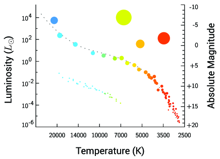
Figure 5: Hertzspring and Russel diagram: luminosity (in terms of the Sun luminosity) as a function of the star temperature. Notice that the temperature increases from right to left. The yellow, orange and red big dots on the right top represent red giants, the blueish sequence on the bottom left represents white dwarfs and the central line is the main sequence, where the red stars are red dwarfs and the blue ones are blue giants.

The main idea underlying nuclear models is to satisfy experimental values and nuclear properties and to achieve this purpose, in almost one century of research, they became more and more sophisticated. The most important of these properties are the binding energy, the saturation density, the symmetry energy, its derivatives and the incompressibility, all of them already explored in the semi-empirical mass formula given in Eq. (4). An important question to be answered is what happens when one moves to higher densities or to finite temperature in the QCD phase diagram shown in Fig. 1 ?

To better understand this point, let’s discuss the concept of nuclear matter. This is a common denomination for an infinite matter characterised by properties of a symmetric nucleus in its ground state, and without the effects of the Coulomb interaction. If one divides eq.(4) by the number of nucleons $A$, one can see that under the conditions just mentioned, the third and forth term disappear. If one assumes an infinite radius, $A\rightarrow\infty$ and no surface effects exist. The pairing interaction would be an unnecessary correction. Hence, the binding energy per nucleon becomes approximately

$$\frac{B(Z,A)}{A}=a_{v}\simeq 16~{}{\rm MeV},$$ (6)

which is what one gets for a two-nucleon system if compared with the average value shown in Fig.3. However, the deuteron binding energy is much smaller, around only 2 MeV. This means that nuclear matter is not an appropriate concept if one wants to describe the properties of a specific nucleus, but it is rather useful to study, for instance, the interior of a neutron star. Normally, it is described by an equation of state, which consists of a set of correlated equations, like pressure, energy and density. The equation of state that describes the ground state of nuclear matter is calculated at zero temperature and is a function of the proton and the neutron densities, which are the same in symmetric matter. Useful definitions are the proton fraction $y_{p}=\frac{\rho_{p}}{\rho}$ and the asymmetry $\delta=\frac{\rho_{n}-\rho_{p}}{\rho}$, which are respectively 0.5 and 0 in the case of symmetric nuclear matter. In these equations $\rho=\rho_{p}+\rho_{n}$ is the total nuclear (or baryonic) density. The macroscopic nuclear energy can be obtained from the microscopic equation of state if one assumes that

$$E_{N}=\int{\cal E}(\rho,\delta)d^{3}{\mathbf{r}},$$ (7)

where ${\cal E}(\rho,\delta)$ is the energy density. Thus,

$$\frac{B(Z,A)}{A}=\frac{E_{N}}{A}-m_{n}=\frac{{\cal E}}{\rho}-m_{n},$$ (8)

where $m_{n}=939$ MeV is the neutron mass ($c=1$). The binding energy as a function of the density is shown in Figure 6. We will see how it can be obtained later in the text. The minimum corresponds to what is generally called saturation density and the value inferred from experiments ranges between $\rho_{0}=0.148-0.17$ fm^-3, as mentioned earlier when the PREX results were given.

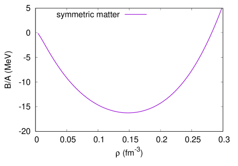
Figure 6: Nuclear matter binding energy per nucleon.

The pressure can be easily obtained from thermodynamics

$$-PV=E_{N}-TS-\mu~{}A,$$ (9)

or, dividing by the volume,

$$-P={\cal E}-T{\cal S}-\mu~{}\rho=\Omega,$$ (10)

where $T$ is the temperature, $\cal S$ is the entropy density, $\mu$ is the chemical potential and $\Omega$ the thermodynamical potential. When we take $T=0$, the expression becomes even simpler because the term $T{\cal S}$ vanishes.

To demonstrate how a simple equation of state (EOS) can be obtained from a relativistic model, we use the free Fermi gas and assume that $\hbar=c=1$, known as natural units. Within this model, the fermions can be either neutrons or nucleons, but I would like to emphasise that it is not adequate to describe nuclear matter properties, as will be obvious later. Its Lagrangian density reads:

$${\cal L}_{0}=\bar{\psi}(i\gamma^{\mu}\partial_{\mu}-m)\psi.$$ (11)

From the Euler-Lagrange equations

$$\partial_{\mu}\left(\frac{\partial{\cal L}}{\partial(\partial_{\mu}\psi)}\right)-\frac{\partial{\cal L}}{\partial\psi}=0,$$ (12)

the Dirac equation is obtained:

$$(i\gamma^{\mu}\partial_{\mu}-m)\psi=0.$$ (13)

Its well known solution has the form $\psi=\Psi(\mathbf{k},\lambda)e^{i(\mathbf{k}\cdot\vec{r}-E(k)t)}$, where $\Psi(\mathbf{k},\lambda)$ is a four-component spinor and $\lambda$ labels the spin. The energy can be calculated from

$$(\vec{\alpha}\cdot\mathbf{k}+\beta M)^{2}\Psi(\mathbf{k},\lambda)=E(\mathbf{k})^{2}\Psi(\mathbf{k},\lambda),$$ (14)

where $\alpha=\gamma_{0}\vec{\gamma}$ or

$$(\mathbf{k})^{2}+M^{2}=E(\mathbf{k})^{2},\quad E(\mathbf{k})=\pm\sqrt{\mathbf{k}^{2}+M^{2}}.$$ (15)

Moreover, one gets

$$<\Psi|\Psi>=\gamma\int\frac{d^{3}k}{(2\pi)^{3}}(f_{+}-f_{-})=\rho,$$ (16)

where $f_{\pm}$ represents the Fermi-Dirac distribution for particles and antiparticles Greiner . For $T=0$, $f_{+}$ is simply the step function and there are no antiparticles in the system. In this case,

$$<\Psi|\Psi>=\gamma\int\frac{d^{3}k}{(2\pi)^{3}}~{}\theta(k_{F}^{2}-k^{2})=$$

$$\frac{\gamma}{2\pi^{2}}\int^{k_{F}}_{0}k^{2}dk=\frac{\gamma~{}k_{F}^{3}}{6\pi^{2}}=\rho,$$ (17)

with $k_{F}$ being the Fermi momentum and $\gamma$ the degeneracy of the particle. If one considers only a gas of neutrons, the degeneracy is 2 due to the spin degeneracy. However, if one considers a gas of nucleons, i.e., symmetric matter with the same amount of protons and neutrons, it is 4 because it accounts for the isospin degeneracy as well.

One can then write

$$<\Psi|\vec{\alpha}\cdot\mathbf{k}+\beta M|\Psi>=\int\frac{d^{3}k}{(2\pi)^{3}}\sqrt{\mathbf{k}^{2}+M^{2}}(f_{+}+f_{-})$$ (18)

or

$${\cal E}=\frac{\gamma}{2\pi^{2}}\int{\mathbf{k}}^{2}dk\sqrt{{\mathbf{k}}^{2}+M^{2}}(f_{+}+f_{-}).$$ (19)

For $T=0$, it becomes

$${\cal E}=\frac{\gamma}{2\pi^{2}}\int^{k_{F}}_{0}{\mathbf{k}}^{2}dk\sqrt{{\mathbf{k}}^{2}+M^{2}}.$$ (20)

As we still do not know the value of the chemical potential in eq.(10), the pressure can be obtained from the energy momentum tensor:

$$T_{\mu\nu}=-g_{\mu\nu}{\cal L}+\partial_{\nu}\psi\left(\frac{\partial{\cal L}}{\partial(\partial^{\mu}\psi)}\right),$$ (21)

having in mind that

$${\cal E}=<T_{00}>,\quad P=\frac{1}{3}<T_{ii}>$$ (22)

and is given by

$$P=\frac{1}{3}\psi^{\dagger}\left(-i\vec{\alpha}\cdot\nabla\right)\psi.$$ (23)

From eq.(18) one can write

$$<\Psi|\vec{\alpha}\cdot\mathbf{k}|\Psi>=k~{}\frac{\partial}{\partial k}<\Psi|\vec{\alpha}\cdot\mathbf{k}+\beta M|\Psi>=$$

$$k~{}\frac{\partial}{\partial k}<\Psi|E(\mathbf{k})|\Psi>$$ (24)

and finally

$$\psi^{\dagger}\left(-i\vec{\alpha}\cdot\nabla\right)\psi=\frac{\gamma}{(2\pi)^{3}}\int d^{3}kk~{}\frac{\partial E}{\partial k}=$$

$$\frac{\gamma}{2\pi^{2}}\int{\mathbf{k}}^{2}dk\cdot\frac{\mathbf{k}^{2}}{\sqrt{\mathbf{k}^{2}+M^{2}}},$$

$$P=\frac{\gamma}{6\pi^{2}}\int dk\frac{\mathbf{k}^{4}}{\sqrt{\mathbf{k}^{2}+M^{2}}}(f_{+}+f_{-}),$$ (25)

and for $T=0$,

$$P=\frac{\gamma}{6\pi^{2}}\int_{0}^{k_{F}}dk\frac{\mathbf{k}^{4}}{\sqrt{\mathbf{k}^{2}+M^{2}}}.$$ (26)

The entropy density of a free Fermi gas is given by

$${\cal S}=-\gamma\int\frac{d^{3}p}{(2\pi)^{3}}\,(f_{+}ln\left(\frac{f_{+}}{1-f_{+}}\right)+ln(1-f_{+})$$ (27)

$$+f_{-}ln\left(\frac{f_{-}}{1-f_{-}}\right)+ln(1-f_{-}))\;,$$ (28)

By minimising eq.(10), the distribution functions are obtained:

$$\frac{\partial\Omega}{\partial f_{+}}=0\rightarrow f_{+}=\frac{1}{1+e^{({\cal E}-\mu)/T}}$$ (29)

and

$$\frac{\partial\Omega}{\partial f_{-}}=0\rightarrow f_{-}=\frac{1}{1+e^{({\cal E}+\mu)/T}}.$$ (30)

On the other hand, the minimisation of the thermodynamical potential with respect to the density yields the chemical potential, i.e.,

$$\frac{\partial\Omega}{\partial\rho}=0\rightarrow\mu.$$ (31)

For $T=0$,

$$\frac{\partial\Omega}{\partial k_{F}}=0\rightarrow\mu=\sqrt{k_{F}^{2}+M^{2}}.$$ (32)

In order to go back to the discussion of nuclear matter, we are lacking exactly the nuclear interaction and its introduction will be seen in section III.

II.2 From the compact objects point of view

I have already discussed the evolution process of a star while it remains in the main sequence of Fig.5. When the fusion ends, it is believed that one of the possible remnants is a neutron star. We see next how it was first predicted and then observed.

In fact, the history of neutron stars started with the observation of a white dwarf and its description with a degenerate free Fermi gas equation of state, as the one just introduced, but with the fermions being electrons instead of neutrons. In 1844, Frederich Bessel observed a very bright star that described an elliptical orbit sirius , known as Sirius. He proposed that Sirius was part of a binary system, whose companion was not possible to see. In 1862, it was observed by Alvan Clark Jr. This companion, named Sirius B, had a luminosity many orders of magnitude lower than Sirius, but approximately the same mass, of the order of the solar mass (1 $M_{\odot}$). In 1914 Walter Adams concluded, through spectroscopy studies that the temperature at the surface of both stars should be similar, but the density of one of them should be much higher than the density of the companion. This high density star was called white dwarf and its properties were explained only in 1926 by Ralph Fowler Fowler , with the help of quantum mechanics. He claimed that the internal constituents of the white dwarf should be responsible for a degeneracy pressure that would compensate the gravitational force. This hypothesis was possible since the electrons are fermions and hence, obey the Pauli Principle. In 1930, Subrahmanyan Chandrasekhar calculated the maximum densities of a white dwarf Chandra and subsequently its maximum mass Chandra2 that he thought should be 0.91 M_⊙ due to an incorrect value of the atomic mass to charge number ratio. It is interesting to note that the correct Chandrasekhar limit, 1.44 M_⊙, was actually obtained by Landau LandauChandra .

Concomitantly, Lev Landau reached the same conclusion as Chandrasekhar and went further: he proposed that even denser objects could exist and in this case, the atomic nuclei would overlap and the star would become a gigantic nucleus Baym . Landau’s hypothesis is considered the first forecast of a neutron star, although the neutrons had not been detected yet. Landau’s paper was written in the beginning of 1931 but published one year later, just when the neutron was discovered by James Chadwick neutrons . The first explicit proposition of the existence of neutron stars was made by Baade and Zwick Baade , soon after Chadwick’s discovery.

In 1939, Toman and, independently Oppenheimer and Volkoff (TOV) tov , used special and general relativity to correct Newton’s equations that described the properties of a perfect isotropic fluid, which they considered could be the interior of compact objects (white dwarfs and neutron stars). While Tolman proposed 8 different solutions for the system of equations, Oppenheimer and Volkoff used the equation of state of a free neutron gas (exactly the one introduced in the last section) and obtained a maximum mass of 0.7 M_⊙ for the neutron star, what was very disappointing because it was lower than the Chandrasekhar limit. However, soon, the limitations of this EOS were noticed: the inclusion of the nuclear interaction could make it harder and then generate higher masses. These calculations will be shown in the next section.

In 1940, Mario Shenberg and George Gamow proposed the Urca process urca , responsible for cooling down the stars by emitting neutrinos, which can carry a large amount of energy with very little interaction.

In 1967, the first neutron star (NS) was detected by Jocelyn Bell and Anthony Hewish seminal . At first, they believed they were capturing signals from an extraterrestrial civilisation and the booklet The Little Green Men really existed. But they soon realised that the radio signals were coming from a compact object with a very stable frequency (pulse) and the object was called pulsar.

It is worth pointing out that white dwarfs and neutron stars bear very different internal constituents and densities. Neutron stars are much denser. This means that general relativity is a very important component in the study of NS, but this is not true for white dwarfs. Hence, it would be expected that only relativistic models, as the ones introduced in the present text, could be used to describe neutron star macroscopic properties. However, there are non-relativistic models, known as Skyrme models which can be used to describe NS, as far as they do not violate causality. Moreover, some non-relativistic models lead to symmetry energies that decrease too much after three times saturation density, which is a very serious problem if we want to apply them to the study of neutron stars, highly asymmetric systems. These problems can be cured with the inclusion of three-body forces, what makes the calculations much more complicated. For a review on Skyrme models, please see ref. skyrme . On the other hand, relativistic models are generally causal and always Lorentz invariant and when extended to finite temperature, anti-particles appear naturally. Thus, only relativistic models are discussed in the present work.

Let’s go back to history because it continues. In 1974 Russel Hulse and Joseph Taylor identified the first binary pulsar PSR1913+16 PSR1913 with a radio-telescope in Arecibo and proposed that the system was losing energy in the form of gravitational waves (GW), the same kind of waves foreseen by relativistic theories. Note that they did not detect gravitational waves directly but instead proved its existence via pulsar timing and were laureated with the Nobel prize for this discovery. In 2015, the first GW produced by two colliding black holes was finally detected directly by LIGO GW15 and in 2017, GW170817, produced by the merger of two NS GW170817 initiated the era of multi-messenger astronomy multi . These gravitational waves have become an excellent source of constraints to the EOS used to describe neutron stars, as will be discussed in a future section.

III Relativistic models for astrophysical studies

In Section II.1 the EOS of a free Fermi gas was introduced and in Section II.2, I mentioned that the EOS can satisfactorily describe a white dwarf, as shown by Chandrasekhar if the free Fermi gas is a gas of electrons. However, if the fermions are neutrons, it cannot describe neutron stars. One important ingredient, besides the already mentioned relativistic effects, is still missing in the recipe: the nuclear interaction. So, let’s go back to nuclear matter.

III.1 The $\sigma-\omega$ model

This model, also known as Walecka model walecka or quantum hadrodynamics (QHD-1) is based on the fact that the interaction inside the nucleus has two contributions: an attractive contribution, at large distances and a repulsive one at short distances, and both can be reasonably well described by Yukawa type potentials and represented by fields generated respectively by scalar and vector mesons. This idea was first proposed by Hans Peter Durr in his Ph.D. thesis in 1956, supervised by Edward Teller, who, in 1955, also proposed a version of the model based on classical field theory johnson . But the quantum version proposed by Walecka was the one that really gained popularity and up to now it is largely applied with different versions and extensions. This simplified model does not take pions into account because, as will be seen next, it is usually solved in a mean field approximation and in this case, the pion contribution disappears. As the $\sigma-\omega$ model is a relativistic model, this simpler and more common approximation is always known as relativistic Mean Field Theory (RMF) or relativistic Hartree approximation.

As the name suggests, the $\sigma-\omega$ model considers that the central effective potential for the nucleon-nucleon interaction is given by

$$V(r)=\frac{g_{\omega}^{2}}{4\pi}\frac{e^{-m_{\omega}r}}{r}-\frac{g_{\sigma}^{2}}{4\pi}\frac{e^{-m_{\sigma}r}}{r},$$

where $r$ is the modulus of the vector that defines the relative distance between two nucleons, the two constants $g_{\sigma}$ and $g_{\omega}$ are adjusted to reproduce the nucleon-nucleon interaction and the meson masses are respectively $m_{\sigma}=550$ MeV and $m_{\omega}=783$ MeV. The interested reader, can look at the potential $V(r)$ obtained with the coupling constants and masses used in this section in livro1 . To obtain the binding energy that corresponds to this potential in RMF, a Lorentz invariant Lagrangian density is necessary and it reads:

$${\cal L}=\bar{\psi}\left[\gamma_{\mu}(i\partial^{\mu}-g_{\omega}\omega^{\mu})-(M-g_{\sigma}\sigma)\right]\psi$$

$$+\frac{1}{2}(\partial_{\mu}\sigma\partial^{\mu}\sigma-m_{\sigma}^{2}\sigma^{2})+\frac{1}{2}m_{\omega}^{2}\omega_{\mu}\omega^{\mu}-\frac{1}{4}F_{\mu\nu}F^{\mu\nu},$$ (33)

where

$$F_{\mu\nu}=\partial_{\mu}\omega_{\nu}-\partial_{\nu}\omega_{\mu},$$ (34)

$\psi$ represents the baryonic field (nucleons), $\sigma$ and $\omega^{\mu}$ represent the fields associated with the scalar and vector mesons and $M$ is the nucleon mass, generally taken as 939 MeV. By comparing eqs. (11) and (33), one can see that besides the Fermi gas representing the nucleons, the latter contains two interaction terms and kinetic and mass terms for both mesons. The usual prescription is to use the Euler-Lagrange equations (12) for each field to obtain the equations of motion. They read:

$$\left(\partial_{\mu}\partial^{\mu}+m_{\sigma}^{2}\right)\sigma=g_{\sigma}\bar{\psi}\psi,$$ (35)

$$\partial_{\mu}F^{\mu\nu}+m_{\omega}^{2}\omega^{\nu}=g_{\omega}\bar{\psi}\gamma^{\nu}\psi$$ (36)

and

$$\left[\gamma_{\mu}(i\partial^{\mu}-g_{\omega}\omega^{\mu})-(M-g_{\sigma}\sigma)\right]\psi=0.$$ (37)

Note that eq. (35) is a Klein-Gordon equation with a scalar source, eq. (36) is analogous to quantum eletrodynamics with a conserved baryonic current ($\bar{\psi}\gamma^{\nu}\psi$), instead of the electromagnetic current and eq.(37) is a Dirac equation for an interacting (not free) gas.

In a RMF approximation, the meson fields are replaced by their expectation values that behave as classical fields:

$$\sigma\rightarrow\left<\sigma\right>\equiv\sigma_{0}$$ (38)

and

$$\omega_{\mu}\rightarrow\left<\omega_{0}\right>\equiv\omega_{0},\quad\left<\omega_{k}\right>=0.$$ (39)

The equations of motion can then be easily solved and they read:

$$\sigma_{0}=\frac{g_{\sigma}}{m_{\sigma}^{2}}<\bar{\psi}\psi>=\frac{g_{\sigma}}{m_{\sigma}^{2}}\rho_{s}$$ (40)

and

$$\omega_{0}=\frac{g_{\omega}}{m_{\omega}^{2}}<\psi^{\dagger}\psi>=\frac{g_{\omega}}{m_{\omega}^{2}}\rho,$$ (41)

where $\rho_{s}$ is a scalar density and $\rho$ is a baryonic number density. The Dirac equation becomes simply

$$\left[(i\gamma_{\mu}\partial^{\mu}-g_{\omega}\gamma_{0}\omega^{0})-(M-g_{\sigma}\sigma_{0})\right]\psi=0,$$ (42)

and

$$M^{*}=M-g_{\sigma}\sigma_{0},$$ (43)

is the effective mass. To obtain the EOS, the recipe is the same as already shown for the free Fermi gas, which leads to expressions for the energy density and pressure. Assuming $C_{s}^{2}=g_{\sigma}^{2}(M^{2}/m_{\sigma}^{2})=267.1$ and $C_{v}^{2}=g_{\omega}^{2}(M^{2}/m_{\omega}^{2})=195.9$, the binding energy $E/N-M=-15.75$ MeV at the saturation density $\rho=0.19$ fm^-3, a little bit too high.

Other important quantities directly related with nuclear matter EOS are the symmetry energy, its derivatives and the incompressibility. The symmetry energy is roughly the necessary energy to transform symmetric matter into a pure neutron matter, as shown in Fig. 7, i.e.,

$${\cal E}(\rho,\delta)\simeq{\cal E}(\rho,\delta=0)+E_{sym}(\rho)\delta^{2}.$$ (44)

Its value can be inferred from experiments and it is of the order of 30-35 MeV and it can be written as

$$E_{sym}=\frac{1}{8}\left(\frac{\partial^{2}({\cal E}/\rho)}{\partial y_{p}^{2}}\right)_{y_{p}=0.5}=\frac{1}{2}\left(\frac{\partial^{2}({\cal E}/\rho)}{\partial\delta^{2}}\right)_{\delta=0}.$$ (45)

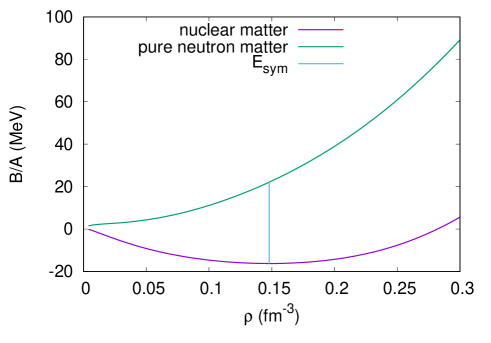
Figure 7: Schematic representation of the nuclear matter symmetry energy.

It is common to expand the symmetry energy around the saturation density in a Taylor series as

$$E_{sym}=J+L_{0}(\frac{\rho-\rho_{0}}{3\rho_{0}})+\frac{K_{sym}}{2}(\frac{\rho-\rho_{0}}{3\rho_{0}})^{2}+{\cal{O}}(3),$$ (46)

where $J$ is the symmetry energy at the saturation point and $L_{0}$ and $K_{sym}$ represent respectively its slope and curvature:

$$L_{0}=3\rho_{0}\left(\frac{\partial E_{sym}(\rho)}{\partial\rho}\right)_{\rho=\rho_{0}},$$ (47)

and

$$K_{sym}=9\rho_{0}^{2}\left(\frac{\partial^{2}E_{sym}(\rho)}{\partial\rho^{2}}\right)_{\rho=\rho_{0}}.$$ (48)

Experimental data for the symmetry energy can be inferred from heavy-ion collisions, giant monopole (GMR) and giant dipole (GDR) resonances, pygmy dipole resonances and isobaric analog states. Accepted values for the slope until very recently lied in between 30.6 and 86.8 MeV relat ; Micaela2017 and for the curvature, in between -400 and 100 MeV Tews ; Zhang . These two quantities are correlated with macroscopic properties of neutron stars, as will be seen later on along this manuscript. Based on 28 experimental and observational data, restricted bands for the values of $J$ ($25<J<35$ MeV) and $L_{0}$ ($25<L_{0}<115$ MeV) were given in bao . More recently, results obtained by the PREX2 experiment PREX2 point to a different band, given by $L_{0}=106\pm 37$ MeV PiekarewiczPREX . If confirmed, this result rehabilitates many of the already ruled out EOS and points to a much larger than previously expected neutron star radius, also discussed later on in the present paper.

Another important quantity is the incompressibility, already mentioned when the liquid drop model idea was introduced. It is a measure of the stiffness of the EOS, i.e., defines how much pressure a system can support and it is calculated from the relation

$$K_{0}=9\left(\frac{\partial P}{\partial\rho}\right)_{\rho=\rho_{0},~{}y_{p}=0.5}$$ (49)

and ranges between 190 and 270 MeV relat ; Micaela2017 . These values can be inferred from both theory and experiments.

I will go back to the importance of these nuclear matter bulk properties and their connection with neutron star properties later on.

III.2 Extended relativistic hadronic models

I next present one example of a complete Lagrangian density that describes baryons interacting among each other by exchanging scalar-isoscalar ($\sigma$) , vector-isoscalar ($\omega$), vector-isovector ($\rho$) and scalar-isovector ($\delta$) mesons:

$$\mathcal{L}=\mathcal{L}_{\rm nm}+\mathcal{L}_{\sigma}+\mathcal{L}_{\omega}+\mathcal{L}_{\rho}+\mathcal{L}_{\delta}+\mathcal{L}_{\sigma\omega\rho},$$ (50)

where Agrawal

$$\mathcal{L}_{\rm nm} = \overline{\psi}(i\gamma^{\mu}\partial_{\mu}-M)\psi+g_{\sigma}\sigma\overline{\psi}\psi-g_{\omega}\overline{\psi}\gamma^{\mu}\omega_{\mu}\psi-\frac{g_{\rho}}{2}\overline{\psi}\gamma^{\mu}\vec{\rho}_{\mu}\cdot\vec{\tau}\psi+g_{\delta}\overline{\psi}\vec{\delta}\cdot\vec{\tau}\psi,$$ (51)

$$\mathcal{L}_{\sigma} = \frac{1}{2}(\partial^{\mu}\sigma\partial_{\mu}\sigma-m^{2}_{\sigma}\sigma^{2})-\frac{A}{3}\sigma^{3}-\frac{B}{4}\sigma^{4},$$ (52)

$$\mathcal{L}_{\omega} = -\frac{1}{4}F^{\mu\nu}F_{\mu\nu}+\frac{1}{2}m^{2}_{\omega}\omega_{\mu}\omega^{\mu}+\frac{C}{4}(g_{\omega}^{2}\omega_{\mu}\omega^{\mu})^{2},$$ (53)

$$\mathcal{L}_{\rho} = -\frac{1}{4}\vec{B}^{\mu\nu}\vec{B}_{\mu\nu}+\frac{1}{2}m^{2}_{\rho}\vec{\rho}_{\mu}\cdot\vec{\rho}^{\mu},$$ (54)

$$\mathcal{L}_{\delta} = \frac{1}{2}(\partial^{\mu}\vec{\delta}\partial_{\mu}\vec{\delta}-m^{2}_{\delta}\vec{\delta}^{2}),$$ (55)

and

$$\mathcal{L}_{\sigma\omega\rho} = g_{\sigma}g_{\omega}^{2}\sigma\omega_{\mu}\omega^{\mu}\left(\alpha_{1}+\frac{1}{2}{\alpha_{1}}^{\prime}g_{\sigma}\sigma\right)+g_{\sigma}g_{\rho}^{2}\sigma\vec{\rho}_{\mu}\cdot\vec{\rho}^{\mu}\left(\alpha_{2}+\frac{1}{2}{\alpha_{2}}^{\prime}g_{\sigma}\sigma\right)$$ (56)

$$+ \frac{1}{2}{\alpha_{3}}^{\prime}g_{\omega}^{2}g_{\rho}^{2}\omega_{\mu}\omega^{\mu}\vec{\rho}_{\mu}\cdot\vec{\rho}^{\mu}.$$

In this Lagrangian density, $\mathcal{L}_{\rm nm}$ represents the kinetic part of the nucleons plus the terms standing for the interaction between them and mesons $\sigma$, $\delta$, $\omega$, and $\rho$. The term $\mathcal{L}_{j}$ represents the free and self-interacting terms of the meson $j$, where $j=\sigma,\delta,\omega,$ and $\rho$. The $\sigma$ self-interaction terms were the first ones to be introduced boguta to correct some of the values of the nuclear bulk properties. The last term, $\mathcal{L}_{\sigma\omega\rho}$, accounts for crossing interactions between the meson fields. The antisymmetric field tensors $F_{\mu\nu}$ and $\vec{B}_{\mu\nu}$ are given by $F_{\mu\nu}=\partial_{\nu}\omega_{\mu}-\partial_{\mu}\omega_{\nu}$ and $\vec{B}_{\mu\nu}=\partial_{\nu}\vec{\rho}_{\mu}-\partial_{\mu}\vec{\rho}_{\nu}-g_{\rho}(\vec{\rho}_{\mu}\times\vec{\rho}_{\nu})$. The nucleon mass is $M$ and the meson masses are $m_{j}$.

In a mean field approximation, the meson fields are treated as classical fields and the equations of motion are obtained via Euler-Lagrange equations. Translational and rotational invariance are assumed. The equations of motion are then solved self-consistently and the energy momentum tensor, Eq. (21) is used in the calculation of the EOS. The calculations follow the steps shown in Section II.1 and III.1. The interested reader can also check them, for instance, in walecka and relat . Nevertheless, some of the important steps are mentioned in what follows. Within a RMF approximation, the common substitution mentioned below is again performed:

$$\sigma\rightarrow\left<\sigma\right>\equiv\sigma_{0},\quad\omega_{\mu}\rightarrow\left<\omega_{0}\right>\equiv\omega_{0},\quad\vec{\rho}_{\mu}\rightarrow\left<\vec{\rho}_{0}\right>\equiv\bar{\rho}_{0(3)},\quad\vec{\delta}\rightarrow\,\,<\vec{\delta}>\equiv\delta_{(3)},$$ (57)

and the equations of motion read:

$$m^{2}_{\sigma}\sigma_{0} =g_{\sigma}\rho_{s}-A\sigma_{0}^{2}-B\sigma_{0}^{3}+g_{\sigma}g_{\omega}^{2}\omega_{0}^{2}(\alpha_{1}+{\alpha_{1}}^{\prime}g_{\sigma}\sigma)+g_{\sigma}g_{\rho}^{2}\bar{\rho}_{0(3)}^{2}(\alpha_{2}+{\alpha_{2}}^{\prime}g_{\sigma}\sigma)\,\mbox{,}\quad$$ (58)

$$m_{\omega}^{2}\omega_{0} =g_{\omega}\rho-Cg_{\omega}(g_{\omega}\omega_{0})^{3}-g_{\sigma}g_{\omega}^{2}\sigma_{0}\omega_{0}(2\alpha_{1}+{\alpha_{1}}^{\prime}g_{\sigma}\sigma_{0})-{\alpha_{3}}^{\prime}g_{\omega}^{2}g_{\rho}^{2}\bar{\rho}_{0(3)}^{2}\omega_{0},$$ (59)

$$m_{\rho}^{2}\bar{\rho}_{0(3)} =\frac{g_{\rho}}{2}\rho_{3}-g_{\sigma}g_{\rho}^{2}\sigma_{0}\bar{\rho}_{0(3)}(2\alpha_{2}+{\alpha_{2}}^{\prime}g_{\sigma}\sigma_{0})-{\alpha_{3}}^{\prime}g_{\omega}^{2}g_{\rho}^{2}\bar{\rho}_{0(3)}\omega_{0}^{2},$$ (60)

$$m_{\delta}^{2}\delta_{(3)} =g_{\delta}\rho_{s3},$$ (61)

and

$$[i\gamma^{\mu}\partial_{\mu}-\gamma^{0}V_{\tau}-(M+S_{\tau})]\psi=0,$$ (63)

where

$$\rho_{s}=\left<\overline{\psi}\psi\right>={\rho_{s}}_{p}+{\rho_{s}}_{n},$$ (64)

$$\rho_{s3}=\left<\overline{\psi}{\tau}_{3}\psi\right>={\rho_{s}}_{p}-{\rho_{s}}_{n},$$ (65)

$$\rho=\left<\overline{\psi}\gamma^{0}\psi\right>=\rho_{p}+\rho_{n},$$ (66)

$$\rho_{3}=\left<\overline{\psi}\gamma^{0}{\tau}_{3}\psi\right>=\rho_{p}-\rho_{n}=(2y_{p}-1)\rho,$$ (67)

with

$${\rho_{s}}_{p,n}=\frac{\gamma M^{*}_{p,n}}{2\pi^{2}}\int_{0}^{{k_{F}}_{p,n}}\frac{k^{2}dk}{\sqrt{k^{2}+M^{*2}_{p,n}}},$$ (68)

$$\rho_{p,n}=\frac{\gamma}{2\pi^{2}}\int_{0}^{{k_{F}}_{p,n}}k^{2}dk=\frac{\gamma}{6\pi^{2}}{k_{F}^{3}}_{p,n},$$ (69)

$$V_{\tau}=g_{\omega}\omega_{0}+\frac{g_{\rho}}{2}\bar{\rho}_{0(3)}\tau_{3},\qquad S_{\tau}=-g_{\sigma}\sigma_{0}-g_{\delta}\delta_{(3)}\tau_{3},$$ (70)

with $\tau_{3}=1$ and $-1$ for protons and neutrons respectively and $\gamma=2$ to account for the spin degeneracy. The proton and neutron effective masses read:

$$M_{p}^{*}=M-g_{\sigma}\sigma_{0}-g_{\delta}\delta_{(3)},$$

$$M_{n}^{*}=M-g_{\sigma}\sigma_{0}+g_{\delta}\delta_{(3)}.$$ (71)

Due to translational and rotational invariance, only the zero components of quadrivectors remain. From the energy-momentum tensor, the following expressions are obtained:

$$\mathcal{E} = \frac{1}{2}m^{2}_{\sigma}\sigma_{0}^{2}+\frac{A}{3}\sigma_{0}^{3}+\frac{B}{4}\sigma_{0}^{4}-\frac{1}{2}m^{2}_{\omega}\omega_{0}^{2}-\frac{C}{4}(g_{\omega}^{2}\omega_{0}^{2})^{2}-\frac{1}{2}m^{2}_{\rho}\bar{\rho}_{0(3)}^{2}+g_{\omega}\omega_{0}\rho+\frac{g_{\rho}}{2}\bar{\rho}_{0(3)}\rho_{3}$$ (72)

$$+ \frac{1}{2}m^{2}_{\delta}\delta^{2}_{(3)}-g_{\sigma}g_{\omega}^{2}\sigma\omega_{0}^{2}\left(\alpha_{1}+\frac{1}{2}{\alpha_{1}}^{\prime}g_{\sigma}\sigma_{0}\right)-g_{\sigma}g_{\rho}^{2}\sigma\bar{\rho}_{0(3)}^{2}\left(\alpha_{2}+\frac{1}{2}{\alpha_{2}}^{\prime}g_{\sigma}\sigma_{0}\right)$$

$$- \frac{1}{2}{\alpha_{3}}^{\prime}g_{\omega}^{2}g_{\rho}^{2}\omega_{0}^{2}\bar{\rho}_{0(3)}^{2}+\mathcal{E}_{\mbox{\tiny kin}}^{p}+\mathcal{E}_{\mbox{\tiny kin}}^{n},$$

with

$$\mathcal{E}_{\mbox{\tiny kin}}^{p,n} = \frac{\gamma}{2\pi^{2}}\int_{0}^{{k_{F}}_{p,n}}k^{2}(k^{2}+M^{*2}_{p,n})^{1/2}dk$$ (73)

and

$$P = -\frac{1}{2}m^{2}_{\sigma}\sigma_{0}^{2}-\frac{A}{3}\sigma_{0}^{3}-\frac{B}{4}\sigma_{0}^{4}+\frac{1}{2}m^{2}_{\omega}\omega_{0}^{2}+\frac{C}{4}(g_{\omega}^{2}\omega_{0}^{2})^{2}+\frac{1}{2}m^{2}_{\rho}\bar{\rho}_{0(3)}^{2}+\frac{1}{2}{\alpha_{3}}^{\prime}g_{\omega}^{2}g_{\rho}^{2}\omega_{0}^{2}\bar{\rho}_{0(3)}^{2}$$ (74)

$$- \frac{1}{2}m^{2}_{\delta}\delta^{2}_{(3)}+g_{\sigma}g_{\omega}^{2}\sigma_{0}\omega_{0}^{2}\left(\alpha_{1}+\frac{1}{2}{\alpha_{1}}^{\prime}g_{\sigma}\sigma_{0}\right)+g_{\sigma}g_{\rho}^{2}\sigma\bar{\rho}_{0(3)}^{2}\left(\alpha_{2}+\frac{1}{2}{\alpha_{2}}^{\prime}g_{\sigma}\sigma\right)$$

$$+ P_{\mbox{\tiny kin}}^{p}+P_{\mbox{\tiny kin}}^{n},\qquad$$

with

$$P_{\mbox{\tiny kin}}^{p,n}=\frac{\gamma}{6\pi^{2}}\int_{0}^{{k_{F}}_{p,n}}\frac{k^{4}dk}{(k^{2}+M^{*2}_{p,n})^{1/2}}.$$ (75)

Table 1: Parameter sets used in this section - all meson masses and $A$ are given in MeV, $\Lambda_{v}={\alpha_{3}}^{\prime}/2$ and $M=939$ MeV.

Model	$m_{\sigma}$	$m_{\omega}$	$m_{\rho}$	$g_{\sigma}$	$g_{\omega}$	$g_{\rho}$	$A$	$B$	$C$	$\Lambda_{v}$
NL3	508.194	782.501	763	10.217	12.868	8.948	2.055 $\times 10^{-3}$	-2.65 $\times 10^{-3}$	0	0
NL3$\omega\rho$	508.194	782.501	763	2.192	12.868	11.276	2.055 $\times 10^{-3}$	-2.65 $\times 10^{-3}$	0	0.03
IUFSU	491.5	782.5	763	9.971	13.032	13.590	1.80 $\times 10^{-3}$	4.9 $\times 10^{-5}$	0.18	0.046

III.3 Too many relativistic models

In relat , a large amount of relativistic models were confronted with two sets of nuclear bulk properties, one more and one less restrictive. The interested reader should check the chosen ranges of properties in both sets and the respective values of 363 models. In what follows, I will restrict myself to 3 parameter sets: NL3 PRC55-540 , NL3$\omega\rho$ Horo , which is an extension of the NL3 parameter set with the introduction of a vector-isovector interaction and IUFSU PRC82-055803 . These models are chosen because they are frequently used in various applications in the literature. Moreover, NL3$\omega\rho$ and IUFSU satisfy all nuclear matter bulk properties, but it will be seen along the text that recent astrophysical observations are not completely satisfied by them. The inclusion of NL3 and its comparison with NL3$\omega\rho$ help the understanding of the importance of the $\omega-\rho$ interaction. Other parameter sets shown along the next sections are GM1 Glen2 , GM3 Glen , TM1 tm1 and FSUGZ03 fsugz03 . All of them are contemplated in relat and the interested reader can check their successes and failures in satisfying the main nuclear bulk properties. Notice that none of the parameter sets explicitly mentioned in the present work includes the $\delta$ meson, which distinguishes protons and neutrons, and consequently, the effective masses given in eq.(71) are identical. The mesonic crossing terms weighted by the parameters $\alpha_{1}$, ${\alpha_{1}}^{\prime}$, $\alpha_{2}$, ${\alpha_{2}}^{\prime}$ are not included either. In Table 1, the parameter values for the three parametrisations mostly used are presented and in Table 2, their main nuclear properties are shown.

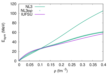
Figure 8: top) Binding energy and bottom) symmetry energy as a function of the baryonic density for the three parameter sets used in this section.

In Figure 8 top, I plot the binding energy per nucleon for the three parameter sets and one can clearly see the slightly different saturation densities and binding energy values. Notice that the $\omega-\rho$ channel does not influence the binding energy of symmetric nuclear matter, but plays an important role in asymmetric matter. In Figure 8 bottom the symmetry energy is depicted and it is easy to see that they are very similar at sub-saturation densities, but completely different at larger densities. As a consequence of what is seen in Figures 8, the incompressibility, the slope and the curvature of the three models are different, as shown in Table 2.

Table 2: Saturation and stellar properties. These values are commented along the text.

Model	$\rho_{0}$	$B/A$	$K_{0}$	$M^{*}/M$	$J$	$L$	$M_{max}/M_{\odot}$	$R_{1.4M_{\odot}}$
	fm-3	MeV	MeV		MeV	MeV		km
NL3	0.148	-16.24	271.53	0.60	37.40	118.53	2.78	14.7
NL3$\omega\rho$	0.148	-16.24	271.60	0.60	31.70	55.50	2.76	13.7
IUFSU	0.155	-16.40	231.33	0.61	31.30	47.21	1.94	12.5

IV Stellar Matter

The idea of this section is to show how the relativistic models presented so far can be applied to describe stellar matter and, in this case, we refer specifically to neutron stars. Looking back at the QCD phase diagram presented in the Introduction, one can see that neutron stars have internal densities that are 6 to 10 times higher than the nuclear saturation density and their temperature is low. Actually, if we compare their thermal energy with the Fermi energy of the system, the assumption of zero temperature is indeed reasonable. At these very high densities the onset of hyperons is expected because their appearance is energetically favourable as compared with the inclusion of more nucleons in the system. To deal with this fact, the first term in the Lagrangian density of eq. (51) has to be modified to take into account, at least, the eight lightest baryons and it becomes:

$$\mathcal{L}_{\rm Bm}=\sum_{B}\overline{\psi_{B}}(i\gamma^{\mu}\partial_{\mu}-M_{B})\psi_{B}+g_{\sigma B}\sigma\overline{\psi_{B}}\psi_{B}-g_{\omega B}\overline{\psi_{B}}\gamma^{\mu}\omega_{\mu}\psi_{B}-\frac{g_{\rho B}}{2}\overline{\psi_{B}}\gamma^{\mu}\vec{\rho}_{\mu}\vec{\tau}\psi_{B}.$$ (76)

The meson-baryon coupling constants are given by

$$g_{jB}=\chi_{Bj}g_{j},$$ (77)

where $g_{j}$ is the coupling of the meson with the nucleon and $\chi_{jB}$ is a value obtained according to symmetry groups or by satisfying hyperon potential values. These are important quantities when hyperons are included in the system Glen ; su3 . We come back to the discussion of these quantities below. If we perform once again a RMF approximation and use the Euler-Lagrange equations to obtain the equations of motion, we find:

$$\sigma_{0}=\sum_{B}\frac{g_{\sigma B}}{m_{\sigma}^{2}}\rho_{sB}-\frac{1}{m_{\sigma}^{2}}\left(A\sigma_{0}^{2}-B\sigma_{0}^{3}\right),$$ (78)

$$\omega_{0}=\sum_{B}\frac{g_{\omega B}}{m_{\omega}^{2}}\rho_{B}-\frac{1}{m_{\omega}^{2}}\left(2\Lambda_{v}g_{\omega}^{2}g_{\rho}^{2}\bar{\rho}_{0(3)}^{2}\omega_{0}\right),$$ (79)

$$\bar{\rho}_{0(3)}=\sum_{B}\frac{g_{\rho B}}{m_{\rho}^{2}}\frac{\tau_{3}}{2}\rho_{B}-\frac{1}{m_{\rho}^{2}}\left(2\Lambda_{v}g_{\omega}^{2}g_{\rho}^{2}\omega_{0}^{2}\bar{\rho}_{0(3)}\right),$$ (80)

where $\rho_{sB}$ is the scalar density and $\rho_{B}$ is the baryon B density, given by:

$$\rho_{sB}=\frac{\gamma}{2\pi^{2}}\int_{0}^{k_{fB}}\frac{M_{B}^{*}}{\sqrt{k^{2}+M_{B}^{*2}}}k^{2}dk\quad,$$ (81)

$$\rho_{B}=\frac{\gamma}{6\pi^{2}}k_{fB}^{3},\quad\mbox{and}\quad\rho=\sum_{B}\rho_{B},$$ (82)

where $k_{fB}$ is the Fermi momentum of baryon $B$. The terms $\mathcal{E}_{\mbox{\tiny kin}}^{p}$ and $\mathcal{E}_{\mbox{\tiny kin}}^{n}$ that appear in eq. (72), must now be substituted by

$$\mathcal{E}_{B}=\frac{\gamma}{2\pi^{2}}\sum_{B}\int_{0}^{k_{fB}}\sqrt{k^{2}+M^{*2}_{B}}k^{2}dk$$ (83)

and

$$M_{B}^{*}=M_{B}-g_{\sigma}\sigma_{0}.$$ (84)

Whenever stellar matter is considered, $\beta$-equilibrium and charge neutrality conditions have to be imposed and hence, the inclusion of leptons (generally electrons and muons) is necessary. These conditions read:

$$\mu_{B}=\mu_{n}-q_{B}\mu_{e},\quad\mu_{e}=\mu_{\mu},\quad\sum_{B}q_{B}\rho_{B}+\sum_{l}q_{l}\rho_{l}=0,$$ (85)

where $\mu_{B}$ and $q_{B}$ are the chemical potential and the electrical charge of the baryons, $q_{l}$ is the electrical charge of the leptons, $\rho_{B}$ and $\rho_{l}$ are the number densities of the baryons and leptons.

After the supernova explosion, the remnant is, at first, a protoneutron star. Before deleptonisation takes place, neutrinos are also present in the system and in this case, the chemical stability condition becomes

$$\mu_{B}=\mu_{n}-q_{B}(\mu_{e}-\mu_{\nu_{e}}),\quad\mu_{e}=\mu_{\mu}.$$ (86)

In this process, entropy is usually fixed at values compatible with simulations of neutron star cooling and the lepton fractions reach values of the order of 0.3-0.4. This scenario is not considered in the present paper, but examples of this calculation can be seen in trapped .

To satisfy the above conditions of chemical equilibrium and charge neutrality, leptons have to be incorporated in the system and this is done with the introduction of a free Fermi gas, i.e.,

$$\mathcal{L}_{lep}=\sum_{l}\bar{\psi}_{l}[i\gamma^{\mu}\partial_{\mu}-m_{l}]\psi_{l},$$ (87)

where the sum runs over the electron and the muon and their eigenenergies are

$$\quad E_{l}=\sqrt{k^{2}+m^{2}_{l}},$$ (88)

so that their energy density becomes

$$\mathcal{E}_{l}=\frac{\gamma}{2\pi^{2}}\sum_{l}\int_{0}^{k_{fl}}\sqrt{k^{2}+m^{2}_{l}}k^{2}dk.$$ (89)

The total pression of the system can be either obtained separately for its baryonic and leptonic parts as in the previous section or by thermodynamics:

$$P=\sum_{f}\mu_{f}\rho_{f}-\mathcal{E}_{f},$$ (90)

where $f$ stands for all fermions in the system and it is common to define the particle fraction (including leptons) as $Y_{f}=\frac{\rho_{f}}{\rho}$.

As already mentioned, an important point is how to fix the meson-hyperon coupling constants $g_{iB},i=\sigma,\omega,\rho$. There are two methods generally used in the literature. The first one is phenomenological and is based on the fitting of the hyperon potentials Glen :

$$U_{Y}=g_{\omega B}\omega_{0}-g_{\sigma B}\sigma_{0},$$ (91)

which, unfortunately, are not completely established. The only well known potential is the $\Lambda$ potential depth $U_{\Lambda}=-28$ MeV Glen2 . Common values for the $\Sigma$ and $\Xi$ potentials are $U_{\Sigma}=+30$ MeV and $U_{\Xi}=-18$ MeV schaffner ; expoy , but their real values remain uncertain. According to Glen2 , appropriate values for the meson hyperon coupling constants defined in eq. (77) are obtained if $\chi_{B\sigma}=0.7$ and $\chi_{B\omega}=\chi_{B\rho}$ is given by 0.772 for NL3 and 0.783 if another common parametrisation, the GM1, is used. However, in these cases, the value of $\chi_{B\rho}$ remains completely arbitrary. We have mentioned GM1 here because it is very often used in the description of neutron star matter since it was one of the first parameter sets with a high effective mass at the saturation density ($M^{*}/M=0.7$) as compared with 0.6 given by NL3, for instance (see Table 2). This high effective mass helps the convergence of the codes when the hyperons are introduced because eq. (84) accounts for a large contribution of the $\sigma_{0}$ field, which in turn, carries the information of the scalar densities of eight baryons. The situation is very different as the one in nuclear matter, where the effective mass only carries the $\sigma_{0}$ field coming from the nucleonic scalar density. This means that whenever the 8 lightest baryons are included, the negative contribution in eq. (84) can make the nucleon mass reach zero very rapidly if the effective mass is too low.

Other examples of how to fit these couplings based on phenomenological potentials can be seen in james1 ; james2 . The second possibility to choose the meson-hyperon couplings is based on the relations established among them by different group symmetries, the most common being SU(3) Weiss ; su3 and SU(6) Luiz2021 .

In the present work we have used the following sets of couplings, for which $U_{\Lambda}=-28$ MeV, $U_{\Sigma}=+30$ MeV and $U_{\Xi}=-18$ MeV:

• for NL3 and NL3$\omega\rho$: $\chi_{\Lambda\sigma}=0.613$, $\chi_{\Sigma\sigma}=0.460$, $\chi_{\Xi\sigma}=0.317$,

• for IUFSU: $\chi_{\Lambda\sigma}=0.611$, $\chi_{\Sigma\sigma}=0.454$, $\chi_{\Xi\sigma}=0.316$,

and $\chi_{\Lambda\omega}=\chi_{\Sigma\omega}=0.667$, $\chi_{\Xi\omega}=0.333$ in all cases due to the SU(6) symmetry and $\chi_{B\rho}=1$ for all hyperons in all cases.

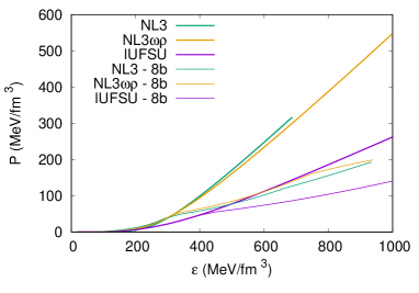
Figure 9: top) Stellar matter EOS obtained with different parametrisations. Thick solid lines show EOS with nucleons only and thin lines represent EOS with the 8 lightest baryons and bottom) same EOS for IUFSU with and without hyperons but with different units for pressure and energy density.

In Fig. 9 six different EOSs are shown, for the three parameter sets identified above, with and without the inclusion of the hyperons. The EOSs for the IUFSU with and without hyperons are reproduced with different units (fm^-4) instead of the more intuitive (MeV/fm³) because those are common units used in stellar matter studies. Notice that $\hbar c=197.326$ MeV.fm and Natural units are used in this calculations.

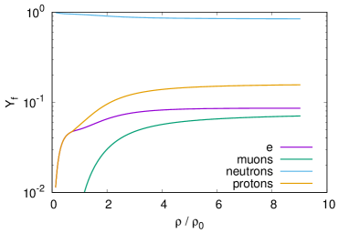
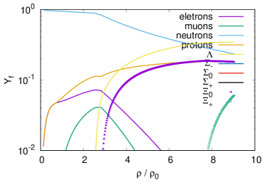
Figure 10: Particle fractions obtained with IUFSU for an EOS with left) nucleons only and right) lightest 8 baryons.

In Fig. 10, the particle fractions obtained with IUFSU are displayed for the two cases shown in Fig.9 right. Notice that when the hyperons are included, these particle fractions depend on the meson-hyperon couplings discussed above. A different choice for these couplings would generate different particle fractions for the same nuclear parametrisation. One can see that the constituents of the neutron stars change with the increase of the density, making their core richer in terms of particles than the region near the crust. From these plots, the conditions of charge neutrality and chemical equilibrium become clear.

IV.1 The Tolman-Oppenheimer-Volkoff equations

As it was just seen, essential nuclear physics ingredients for astrophysical calculations are appropriate equations of state (EOS). After the EOSs are chosen, they enter as input to the Tolman-Oppenheimer-Volkoff equations (TOV) tov , which in turn, give as output some macroscopic stellar properties: radii, masses and central energy densities. Static properties, as the moment of inertia and rotation rate can be obtained as well. The EOSs are also necessary in calculations involving the dynamical evolution of supernova, protoneutron star evolution and cooling, conditions for nucleosynthesis and stellar chemical composition and transport properties, for instance.

The TOV equations were obtained by Tolman and independently by Oppenheimer and Volkoff tov , as already mentioned, and they read:

$$\frac{dP}{dr}={} -G\frac{({\cal E}+P)(M(r)+4\pi Pr^{3})}{r^{2}-2M(r)r},$$ (92)

$$={} -\frac{G{\cal E}M(r)}{r^{2}}\left[1+\frac{P}{{\cal E}}\right]\left[1+\frac{4\pi r^{3}P}{M(r)}\right]\left[1-\frac{2GM(r)}{r}\right]^{-1}$$

$$\frac{dM}{dr}={} 4\pi{\cal E}r^{2},$$

$$\frac{dM_{Baryonic}}{dr}={} 4\pi m_{n}r^{2}\rho(r)\left[1-\frac{2M(r)}{r}\right]^{-1/2},$$

where $M$ is the gravitational mass, $M_{Baryonic}$ the baryonic mass, $m_{n}$ is the nucleon mass and $r$ is the radial coordinate and also the circumferential radius. Be aware that $M_{Baryonic}$ refers to the baryonic mass of the star and it is not the same as the $M_{B}$, the individual baryonic masses used to compute the EOS.

The first differential equation is also shown in such a way that the corrections obtained from special and general relativity are clearly separated.

The EOSs shown on the r.h.s. of Fig. 9 are then used as input to the above TOV equations and the corresponding mass-radius diagram is shown in Fig. 11. Each curve represents a family of stars, being the maximum point of the curves related to the maximum stellar mass of the family. By comparing the curves shown in Fig. 9 and Fig. 11, one can clearly see that the harder EOS yields higher maximum mass. Hence, the inclusion of hyperons makes the EOS softer, as expected, but results in lower maximum masses. As there is no reason to believe that the hyperons are not present, this connection of softer EOS with lower neutron star mass gave rise to what is known as the hyperon puzzle. I will go back to this debate in the next section.

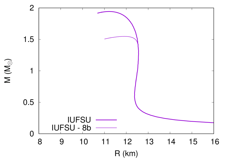
Figure 11: Mass-radius diagram obtained with the IUFSU parametrisation for hadronic matter with (8b) and without hyperons.

I would like to call the attention of the reader for the values of the symmetry energy slope ($L_{0}$), which has been extensively discussed in the last years. Although its true value is still a matter of debate, most studies indicate that it has non-negligible implications on the neutron star macroscopic properties Rafa ; Lopes2014 ; Tsang ; Micaela2017 ; Lattimer2014 ; Pais2016 ; Dex2019 ; Prov2019 . The slope can be controlled by the inclusion of the $\omega-\rho$ interaction, as can be seen in Table 2. In general, the larger the value of the interaction, the lower the values of the symmetry energy and its slope Rafa . As a general trend, it is also true that the lower the value of the slope, the lower the radius of the canonical star, the one with 1.4 $M_{\odot}$. In Table 2 the values of the maximum stellar masses obtained without the inclusion of hyperons and the radii of the canonical stars are displayed. Notice, however, that the value of the radius of the canonical stars depends on the EOS of the crust. To obtain the values shown in Table 2, I used the BPS EOS bps for the outer crust and interpolated the inner crust. As far as the maximum mass is concerned, the crust barely affects it, since the involved densities are too low. I will discuss this subject further when discussing the pasta phase in Section IV.3. Another interesting correlation noticed in isaac2014 is that the onset of the charged (neutral) hyperons takes place at lower (larger) densities for smaller values of the slope.

IV.2 Structure of neutron stars and observational constraints

Although the internal constitution of a neutron star cannot be directly tested, it is reasonably well understood. A famous picture of the NS internal structure was drawn by Dany Page and can be seen in Lattimer2004 . Close to the surface of the star, there is an outer and an inner crust and towards the center, an outer and an inner core are believed to exist. The solid crust is expected to be formed by nonuniform neutron rich matter in $\beta$-equilibrium. This inhomogeneous phase is known as pasta phase and calculations predict that it exists at densities lower than 0.1 fm^-3, where nuclei can coexist with a gas of electrons and neutrons which have dripped out. The center of the star is composed of hadronic matter and the true constituents are still a matter of debate, as one can conclude from the results presented in the last section. The fact that the core should contain hyperons is widely accepted, although this possibility excludes many EOS that become too soft to explain the existing massive stars, namely, MSP J0740+6620, whose mass range lies at $2.07\pm 0.08~{}M_{\odot}$  Cromartie ; NICER_news , PSR J0348+0432 with mass of $2.01\pm 0.04~{}M_{\odot}$ Antoniadis and PSR J1614-2230, which is also a massive neutron star Demorest . Until around 2005, these massive NS had not been detected and practically all EOS could satisfy a maximum 1.4 $M_{\odot}$ star.

Since the appearance of hyperons is energetically favorable, different possibilities were considered in the literature so that the EOS would be stiffer, as the tuning of the unknown meson-hyperon coupling constants, for an example. Another mechanism that increases the maximum mass of neutron stars with hyperons in their core is the inclusion of an additional vector meson that mediates the hyperon-hyperon interaction su3 ; Weiss . In Fig. 12, mass-radius curves are shown for different hyperon-meson coupling constants of the GM1 parametrisation su3 . One can see that all choices produce results with high maximum masses, satisfying the new massive star constraints. I refer the reader to su3 and references therein for explanations on the introduction of the strange meson channel on the Lagrangian density and the corresponding strange meson-hyperon couplings.

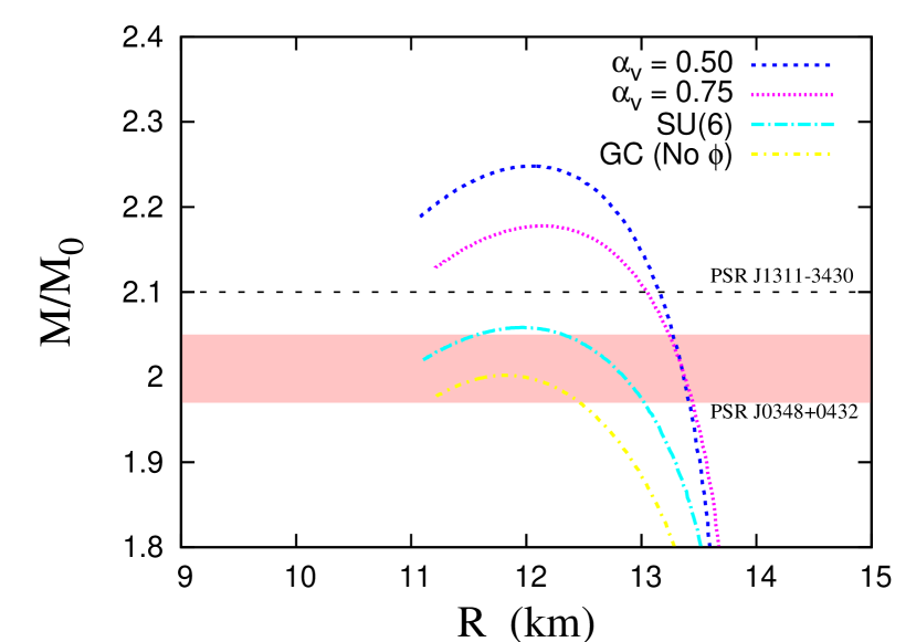
Figure 12: Mass-radius curve for the GM1 parametrisation based on su3 .

As already mentioned in Sec. II.2, the observation of the binary neutron star system GW170817 GW170817 by the LIGO-Virgo scientific collaboration and also in the X-ray, ultraviolet, optical, infrared, and radio bands gave rise to the new era of multi-messenger astronomy multi . The detection of the corresponding gravitational wave helped the establishment of additional constraints to the physics of neutron stars. This subject is better discussed next, but at this point, I would like to mention that a series of papers based on the these constraints imposed restricted values for the neutron star radius Annala2018 ; Ozel2018 ; Riley2019 ; Miller2019 ; Capano2020 , not always compatible among themselves.

The dimensionless tidal deformability, also called tidal polarisability and its associated Love number are related to the induced deformation that a neutron star undergoes by the influence of the tidal field of its neutron star companion in the binary system. The idea is analogous to the tidal response of our seas on Earth as a result of the Moon gravitational field. The theory of Love numbers emerges naturally from the theory of tidal deformation and the first model was proposed in 1909 by Augustus Love firstLove based on Newtonian theory. The relativistic theory of tidal effects was deduced in 2009 Damour ; Binn and since then the computing of Love numbers of neutron stars has become a field of intense investigation.

As different neutron star EOS and related composition have different responses to the tidal field, the tidal polarisability can be used to discriminate between different equations of state. A complete overview on the theory of Love numbers in both Newtonian and General Relativity theories can be found in cesar2020 . Here, I show next only the main equations for the understanding of the constraints on NS.

The second order Love number $k_{2}$ is given by

$$k_{2}=\frac{8C^{5}}{5}(1-2C)^{2}[2+C(y_{R}-1)-y_{R}]\times$$

$$\times\Big{\{}2C[6-3y_{R}+3C(5y_{R}-8)]$$

$$+4C^{3}[13-11y_{R}+C(3y_{R}-2)+2C^{2}(1+y_{R})]$$

$$+3(1-2C^{2})[2-y_{R}+2C(y_{R}-1)]{\rm ln}(1-2C)\Big{\}}^{-1}.$$ (93)

where $C=M/R$ is the star compactness, $M$ and $R$ are the total mass and total circumferential radius of the star respectively and $y_{R}=y(r=R)$, which is obtained from

$$r\frac{dy}{dr}+y^{2}+yF(r)+r^{2}Q(r)=0.$$ (94)

Here the coefficients are given by

$$F(r)=[1-4\pi r^{2}({\cal E}-P)]/E$$ (95)

and

$$Q(r)= 4\pi\left[5{\cal E}+9P+({\cal E}+P)\left(\frac{\partial P}{\partial{\cal E}}\right)-\frac{6}{4\pi r^{2}}\right]/E$$

$$-4\left[\frac{m+4\pi r^{3}P}{r^{2}E}\right]^{2},$$ (96)

where $E=1-2m/r$, ${\cal E}$ and $P$ are the energy density and pressure profiles inside the star. Notice that Eq. (94) has to be solved coupled to the TOV equations.

Finally, one can obtain the dimensionless tidal deformability $\Lambda$, which is connected to the compactness parameter $C$ through

$$\Lambda=\frac{2k_{2}}{3C^{5}}.$$ (97)

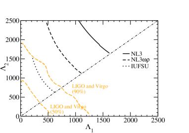
Figure 13: top) Love number as a function of the compactness and bottom) Tidal deformabilities of both NS in the binary system before the merger.

In Fig. 13, the second order Love number as a function of the compactness is shown for the 3 equations of state discussed in Section III.2, as well as the corresponding tidal deformabilities $(\Lambda_{1},\Lambda_{2})$ for the binary system ($M_{1},M_{2}$), with $M_{1}>M_{2}$. The plots are calculated from the equation for the chirp mass

$$M_{chirp}=(M_{1}M_{2})^{3/5}(M_{1}+M_{2})^{-1/5},$$ (98)

and the diagonal dotted line corresponds to the case $M_{1}=M_{2}$. The lower and upper dashed lines correspond to LIGO/Virgo collaboration 50$\%$ and 90$\%$ confidence limits respectively, which are obtained from the GW170817 event. The EOS used to obtain these curves do not include hyperons to avoid the uncertainties related to the meson-hyperon couplings. It is important to mention the matching procedure used to compute the Love number and the tidal polarisabilities. The outer crust is a BPS EOS, the inner crust is a polytropic function which interpolates between the outer crust and the core. A detailed explanation is given in skyrmeGW , sections 2.2 and 2.3. More advanced crustal EOSs are available Pearson2020 ; Fantina and I discuss the sensitivity of some results on the crust model later on. One can see from these figures that the Love numbers are very different for the three models and so are the tidal polarisabilities, the NL3 and NL3$\omega\rho$ not being able to reproduce the GW170817 data satisfactorily. Actually, this behaviour of the NL3 and NL3$\omega\rho$ had already been observed in constanca2018 , but one should notice that in constanca2018 , the confidence lines were taken from a preliminary version of the LIGO/Virgo data GW170817 while in the present paper, they are taken from GW170817_new , where the consideration of massive stars was neglected.

Another important constraint concerns the radii of the canonical stars, the ones with $M=1.4$ M_⊙. According to the LIGO/Virgo collaboration, the tidal polarisability of canonical stars should lie in the range $70\leq\Lambda_{1.4}\leq 580$ GW170817_new , a restriction that imposed a constraint to the radii of the corresponding stars, which should lie in the range $10.5$ km $\leq R_{1.4M_{\odot}}\leq 13.4$ km. This constraint, which does not take into account a maximum stellar mass of 1.97 M_⊙, only excludes the NL3 parameter set from the ones we are analysing (see Table 2), exactly the one that was shown not to describe nuclear bulk properties well enough. But…the history has become more complicated: a recently published paper concludes that the canonical neutron star radius cannot be larger than 11.9 km Capano2020 . If such small radius is confirmed, it could imply in a revision of the EOSs or of the gravity theory itself, as done in Clesio . Notice, however, that this small radius is in line with older works that predicted that the maximum mass of a canonical star should be 13.6 km Annala2018 and Ozel2018 , whose authors claimed that any NS, independently of its mass, should bear a radius smaller than 13 km. Moreover, the new information sent by NICER NICER_news supports the evidence that the detected massive PSR J0740+6620 has a radius of the order of $12.35\pm 0.75$ km and that a star with a mass compatible with a canonical star, J0030+0451, has a radius of the order of $12.45\pm 0.65$ km NICER_canonical , or $12.71^{+1.14}_{1.19}$ km Riley2019 or even $13.02^{+1.24}_{1.06}$ km Miller2019 , depending on the analysis performed. These recent detections point to the fact that the radii of canonical and massive stars are of the same order and this feature is not easily reproduced by most EOSs. On the other hand, one of the analysis of the results from the PREX experiment implies that $13.25$ km $\leq R_{1.4M_{\odot}}\leq 14.26$ km corresponding to a tidal polarisability in the range $642\leq\Lambda_{1.4M_{\odot}}\leq 955$ PiekarewiczPREX , also much higher than the above mentioned value obtained from GW170817 data. Notice, however, that the recent PREX results seem to contradict previous understandings on the softness of the symmetry energy Piekarewiczpola . Hence, the sizes of these objects are still a source of debate. One of the conclusions in PiekarewiczPREX is that a precise knowledge of the crust of these compact objects may help to minimize the systematic uncertainties of these results.

A detailed analysis of the relativistic mean field models shown to be consistent with all nuclear bulk properties in relat according to the masses and radii they yield when applied to describe NS, can be found in NS_RMF . Thirty four models were analysed and only twelve were shown to describe massive stars with maximum masses in the range $1.93\leq M/M_{\odot}\leq 2.05$ without the inclusion of hyperons. In another paper GW_RMF , the very same models were confronted with the constraints imposed by the LIGO/Virgo collaboration. In this case, 24 models were shown to satisfy them. However, only 5 models could, at the same time describe massive stars and constraints from GW170817. These studies did not use EOSs with hyperons, what poses an extra degree of complication due to the uncertainties on the meson-hyperon coupling constants. Looking at the three sets used in the present work, one can clearly see the difficulty. The two models that can describe massive stars are outside the range of validity of the GW170817 tidal deformabilities. On the other hand, IUFSU gives a mass a bit lower than desired, a deficiency that can be correct with some tuning.

Another aspect that deserves to be mentioned refers to the inclusion of $\Delta$ baryons in the EOS. If they are considered as a possible constituent of neutron stars, at least with the parametrisations studied (GM1 and GM1$\omega\rho$), no “$\Delta$ puzzle” is observed Veronica_Kauan .

IV.3 The importance of the inner and outer crusts

When examining neutron star merger, the coalescence time is determined by the tidal polarisability, which as already explained, is a direct response of the tidal field of the companion that induces a mass quadrupole. This scenario suggests that the neutron star crust should play a role in this picture. If one looks at the famous figure drawn by Dany Page Lattimer2004 , one can see that the crust is divided in two pieces, the outer and the inner crust, the latter being the motive for the present section. It may include a pasta phase, the result of a frustrated system in which there is a unique competition between the Coulomb and the nuclear interactions, possible at very low baryonic densities. In the simplest interpretation of the geometries present in the pasta phase, they are known as droplets (3D), rods (2D) and slabs (1D) and their counterparts (bubbles, tubes and slabs) are also possible. Much more sophisticated geometries such as waffles, parking garages and triple periodic minimal surface have been proposed schneider2018 ; newton2009 ; schuetrumpt2019 , but I next describe only the more traditional picture.

The pasta phase is the dominant matter configuration if its free energy (binding energy at $T=0$) is lower than its corresponding homogeneous phase. Depending on the model, the used parametrisation and the temperature pasta , typical pasta densities lie between 0.01 and 0.1 fm^-3. Different approaches are used to compute the pasta phase structures: the coexisting phases (CP) method, the Thomas-Fermi approximation, numerical simulations, etc. For detailed calculations, one can look at pasta , maruyama , Schneider2016 , for instance. In what follows, I only show the main equations used to build the pasta phase with the CP method.

According to the Gibbs conditions, both pasta phases have the same pressure and chemical potentials for proton and neutron and, at a fixed temperature, the following equations must be solved simultaneously:

$$P^{I}=P^{II},$$ (99)

$$\mu_{p}^{I}=\mu_{p}^{II},$$ (100)

$$\mu_{n}^{I}=\mu_{n}^{II},$$ (101)

$$f(\rho^{I}_{p}-\rho_{e})+(1-f)(\rho^{II}_{p}-\rho_{e})=0.$$ (102)

where $I$ ($II$) represents the high (low) density region, $\rho_{p}$ is the global proton density, $\rho_{e}$ is the electron density taken as constant in both phases and $f$ is the volume fraction of the phase $I$, that reads

$$f=\frac{\rho-\rho^{II}}{\rho^{I}-\rho^{II}}.$$ (103)

The total hadronic matter energy reads:

$${\cal E}_{matter}=f{\cal E}^{I}+(1-f){\cal E}^{II}+{\cal E}_{e},$$ (104)

where ${\cal E}^{I}$ and ${\cal E}^{II}$ are the energy densities of phases $I$ and $II$ respectively and ${\cal E}_{e}$ is the energy density of the electrons, included to account for charge neutrality. The total energy can be obtained by adding the surface and Coulomb terms to the matter energy in Eq. (104),

$${\cal E}={\cal E}_{matter}+{\cal E}_{surf}+{\cal E}_{Coul}.$$ (105)

Minimizing ${\cal E}_{surf}+{\cal E}_{Coul}$ with respect to the size of the droplet/bubble, cylinder/tube or slabs, we obtain maruyama ${\cal E}_{surf}=2{\cal E}_{Coul}$ where

$${\cal E}_{Coul}=\frac{2\alpha}{4^{2/3}}(e^{2}\pi\Phi)^{1/3}\left[\sigma^{surf}D(\rho^{I}_{p}-\rho^{II}_{p})\right]^{2/3},$$ (106)

with $\alpha=f$ for droplets, rods and slabs, and $\alpha=1-f$ for tubes and bubbles. The quantity $\Phi$ is given by

$$\Phi=\left\{\begin{array}[]{c}\left(\frac{2-D\alpha^{1-2/D}}{D-2}+\alpha\right)\frac{1}{D+2},\quad D=1,3\\ \frac{\alpha-1-\ln\alpha}{D+2},\quad D=2\end{array}\right.$$ (109)

where, $\sigma^{surf}$ is the surface tension, which measures the energy per area necessary to create a planar interface between the two regions. The surface tension is a crucial quantity in the pasta calculation and it is normally parametrised with the help of more sophisticated formalisms. Another important aspect is that the pasta phase is only present at the low-density regions of the neutron stars, and in this region, muons are not present, although they are present in the EOS that describes the homogeneous region.

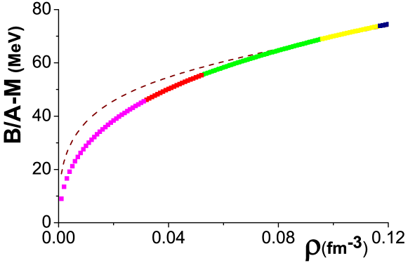
Figure 14: $npe$ matter binding energy obtained with the CP method and NL3 parametrisation PRC55-540 . Figure taken from pasta .

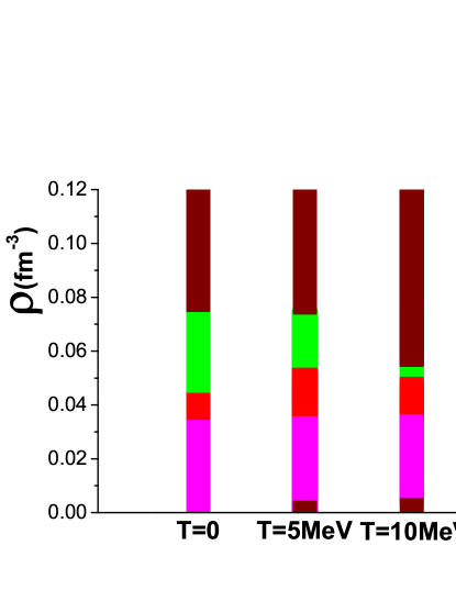
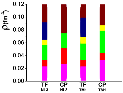
Figure 15: Phase diagrams obtained with Left) NL3 parametrisation and CP method for $Y_{p}=0.5$. From bottom to top the colors represent homogeneous phase ($T=5$ and 10 MeV only), droplets, rods and homogeneous phase. Right) NL3 and TM1 parametrisations with CP and TF methods for $Y_{p}=0.3$ and $T=0$. Figures taken from pasta .

In Fig. 14, I plot the binding energy of the homogeneous matter (dashed line) as compared with the pasta phase binding energy (solid line with different colours representing the different structures). One can see that the pasta phase binding energy is lower up to a certain density, when the homogeneous phase becomes the preferential state. In Fig. 15, I show various phase diagrams obtained with the CP and TF methods for fixed proton fractions at different temperatures. As the temperature increases, the pasta phase shrinks. Here I have mentioned the TM1 parameter set tm1 , not used before in the present work, but also quite common in the literature. The purpose is only to show that different approximations and different parametrisations result in different internal structures with different transition densities from one phase to another.

But then, what is the influence of the pasta phase on the calculation of the tidal polarisability and if this structure is not well determined, how much its uncertainty contributes to the final calculations? This problem was tackled in GW_QMC and, as the model used in that paper is quite different from the RMF models we use in the present work, we do not include any figures, but it is fair to say that the contribution is indeed minor. In GW_QMC , the BPS EOS was used for the outer crust. For the inner crust, two possibilities were considered: the existence of the pasta phase and a simple interpolation between the outer crust and the core. It was observed that, although the explicit inclusion of the pasta phase affected the Love number in a visible way, it almost did not change the tidal polarisabilities, a result that corroborated the findings in piekarewicz . These results can be explained by the fact that, for a fixed compactness, even if the Love number is sensitive to the inner crust structure, the tidal polarisability scales with the fifth power of $C$ and hence, the influence is small.

And what about the outer crust? Indeed, in this case, the tidal effects should be even more sensitive. In what follows, I test how much the use of a modern EOS for the outer crust, which we call reliable Fantina change the results as compared with the BPS generally used and mentioned below. A modified version of the IUFSU model known as FSUGZ03 fsugz03 was used to plot Figure 16 and we trust the qualitative results would be the same for any other parametrisation. In this Figure, the outer crust is linked directly to the core EOS, as seen on the top. Log-scale is used because the differences cannot be seen in linear scale. Then, the different prescriptions are used to compute the tidal polarisabilities shown on the bottom. Once again, one can see that the influence is very small.

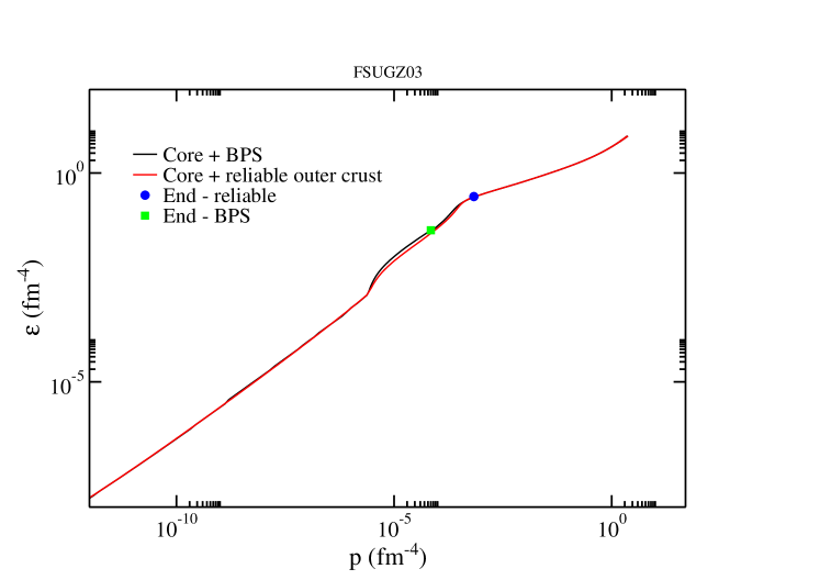
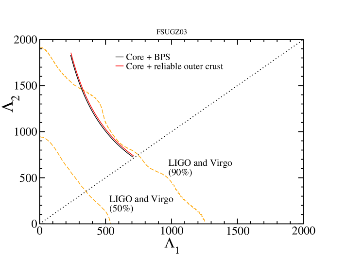
Figure 16: top) EOSs obtained with the outer crust described by BPS and by a reliable model Fantina ; bottom) Tidal polarisabilities for both NSs with the EOSs shown on the right.

Although we have seen that neither the outer nor the inner crust alter significantly the tidal polarisabilities, they do have an impact, which was quantified in marcio1 ; marcio2 . The authors of these works concluded that the impact of the crust EOS is not larger that 2%, but the matching procedure (crust-core) can account for a 5% difference on the determination of the low mass NS radii and up to 8% on the tidal deformability. In another recent work Luiz_crust , the inner crust was parametrised in terms of a polytropic-like EOS and the sound velocity and canonical star radii were computed. EOS for the inner crust with different sound velocities produced radii with up to 8% difference when the same EOS was used for the core.

Albeit the fact that present results show that the inclusion of the pasta phase is not essential when the above discussed macroscopic properties of NSs are computed, it may indeed be important for the thermal thermal , magnetic evolution magnetic1 ; magnetic2 and neutrino diffusion of NS opacity1 ; opacity2 , processes that take place at different epochs. Hence, being able to handle properly the pasta phase structure is still a matter or concern. The first issue worth discussing is the possible existence of baryons that are more massive than nucleons and carry strangeness in the pasta phase. In hyperons , it was verified that the $\Lambda$ hyperons, can indeed be present, although in small amounts, as seen in Fig.17, where the $\Lambda$ fraction is shown as a function of temperature in phases $I$ (clusters) and $II$ (gas). For the parametrisation used, NL3$\omega\rho$, the pasta phase disappears at T=14.45 MeV, the $\Lambda$s being present for electron fractions ranging from 0.1 to 0.5 and in quantities larger than $10^{-11}$ for $T>7$ MeV. The $\Xi^{-}$ can also be found, but in much smaller amounts, of the order of $10^{-12}$.

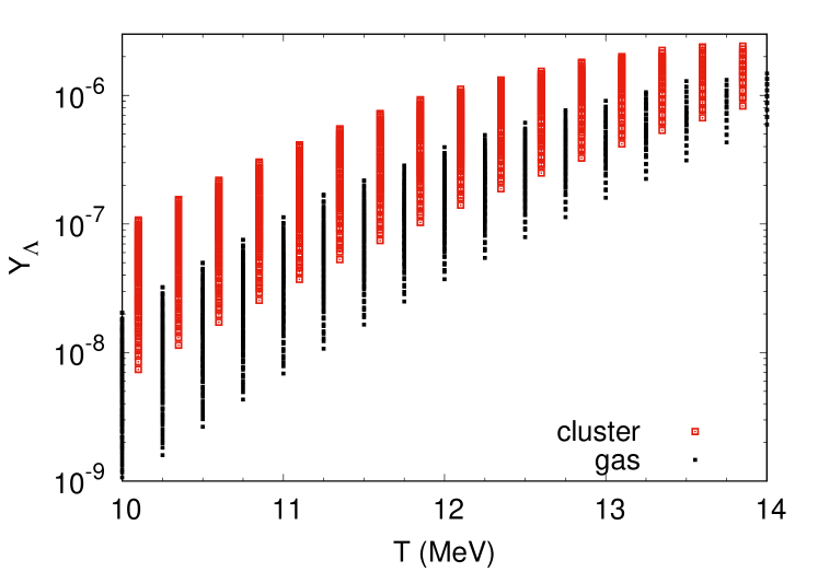
Figure 17: $\Lambda$ fraction as a function of temperature in the cluster and gas phases with the NL3$\omega\rho$ parametrisation Horo . Figure taken from hyperons .

The second important point refers to the fact that the CP method just presented and also another commonly used method, the Thomas-Fermi approximation TF , can only provide one specific geometry for each density, temperature and proton (or electron) fraction but it is well known that this picture is very naive. In fact, different geometries can coexist at thermal equilibrium maruyama2013 ; Schneider2016 ; Fattoyev2017 . The problem with these more sophisticated approaches is that the computational cost is tremendous, making them inadequate to be joined to other expensive computational methods that may be necessary to calculate neutrino opacities and transport properties, for instance. In a recent paper, a prescription with a very low computational cost was presented flu . In that paper, fluctuations are taken into account in a reasonably simple way by the introduction of a rearrangement term in the free energy density of the cluster. A simple result can be seen in Figure 18, where one can see that different geometries can coexist at a certain temperature for a fixed density. If different proton fractions are considered, the dominat geometry changes as in the CP or TF method, but the other geometries can still be present. The complete formalism has been revised and extended to asymmetric matter and can be found in flu2 .

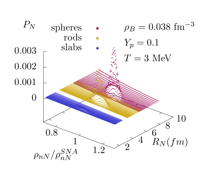
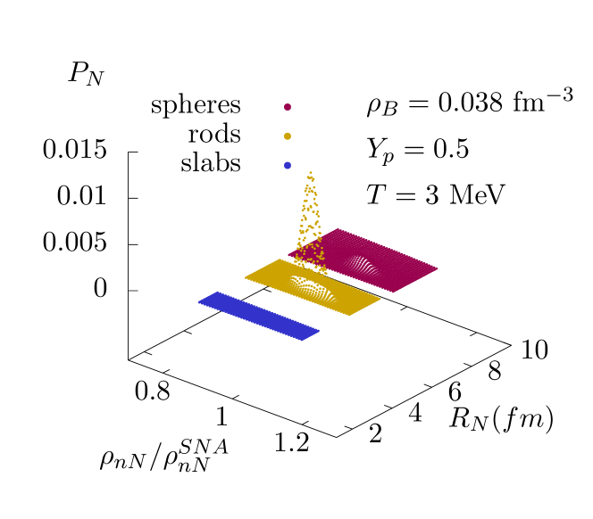
Figure 18: 3D probability distribution as a function of the pasta linear dimension and the normalised cluster density with different geometries obtained with the IUFSU parametrisation for different proton fractions. Notice the vertical scale differences.

V Hybrid stars

So far, I have discussed the possibility that hadronic matter exists in the core of a neutron star and that nuclear physics underlies the models that describe it. The idea of a hybrid star, containing a hadronic outer core that has a different composition than the inner core, which could be composed of deconfined quarks was first proposed by Ivanenko and Kurdgelaidze firsthybrid in the late 60’s. In their papers, they have even foreseen that a transition to a superconducting phase would be possible. This idea has gained credibility lately. A model-independent analysis based on the sound velocity in hadronic and quark matter points to the fact that the existence of quark cores inside massive stars should be considered the standard pattern nature_2020 . In this case, one would be dealing with what is known as hybrid star and, from the theoretical point of view, its description requires a sophisticated recipe: a reliable model for the outer hadronic core and another model for the inner quark core. The ideal picture would be a chiral model that could describe both matters as density increases, but those models are still rarely used veronica1 ; veronica2 ; Lena2016 ; Clebson19 . Generally, what we find in the literature are Walecka-type models as the ones presented in Section III.2 or density-dependent models, whose density dependence is introduced on the meson-baryon couplings as in DDHD ; Typel for the hadronic matter and the MIT bag model mit or the Nambu-Jona-Lasinio (NJL) model njl for the quark matter. While the MIT bag model is very simplistic, the NJL model is more robust and accounts for the expected chiral symmetry but cannot satisfy the condition of absolutely stable strange matter that will be discussed next. The MIT bag model EOS is simply the EOS calculated for a free Fermi gas in Section II.1, where the masses are the ones of the $u,d,s$ quarks, generally taken as $m_{u}=m_{d}=5$ MeV and $m_{s}$ varying from around 80 to 150 MeV and the inclusion of a bag constant $B$ of arbitrary value, which is responsible for confining the quarks inside a certain surface. $B$ enters with a negative sign in the pressure equation and consequently a positive one in the energy density equation. The NJL EOS is more complicated and besides accounting for chiral symmetry breaking/restoration, also depends on a cut-off parameter. The derivation of the EOS can be obtained in the original papers njl , in an excellent review article buballa_review or in one of the papers I have co-authored as DC2003 , for instance and I will refrain from copying the equations here. Contrary to the MIT bag model, the NJL model does not offer the possibility of free parameters. All of them are adjusted to fit the pion mass, its decay constant, the kaon mass and the quark condensates in the vacuum. There are different sets of parameters for describing the SU(2) (only considers $u$ and $d$ quarks) and the SU(3) versions of the model.

When building the EOS to describe hybrid stars, two constructions are comonly made: one with a mixed phase (MP) and another without it, where the hadron and quark phases are in direct contact. In the first case, neutron and electron chemical potentials are continuous throughout the stellar matter, based on the standard thermodynamical rules for phase coexistence known as Gibbs conditions. In the second case, the electron chemical potential suffers a discontinuity and only the neutron chemical potential is continuous. This condition is known as Maxwell construction. The differences between stellar structures obtained with both constructions were discussed in many papers maruyama07 ; vos2 ; paoli and I just reproduce the main ideas next.

In the mixed phase, constituted of hadrons and quarks, charge neutrality is not imposed locally but only globally, meaning that quark and hadron phases are not neutral separately. Instead, the system rearranges itself so that

$$\chi\rho_{c}^{QP}+(1-\chi)\rho_{c}^{HP}+\rho_{c}^{l}=0,$$

where $\rho_{c}^{iP}$ is the charge density of the phase $i=H,Q$, $\chi$ is the volume fraction occupied by the quark phase, and $\rho_{c}^{l}$ is the electric charge density of leptons. The Gibbs conditions for phase coexistence impose that Glen :

$$\mu^{HP}_{n}=\mu^{QP}_{n},\quad\mu^{HP}_{e}=\mu^{QP}_{e}\quad{\rm and}\quad P^{HP}=P^{QP},$$

and consequently,

$$\langle{\cal E}\rangle=\chi{\cal E}^{QP}+(1-\chi){\cal E}^{HP}+{\cal E}^{l}$$ (110)

and

$$\langle\rho\rangle=\chi\rho^{QP}+(1-\chi)\rho^{HP}.$$ (111)

The Maxwell construction is much simpler than the case above and it is only necessary to find the transition point where

$$\mu^{HP}_{n}=\mu^{QP}_{n}\quad{\rm and}\quad P^{HP}=P^{QP},$$

and then construct the EoS.

In Fig.19, different EOS are built with both constructions and the respective mass radius curves are also shown. In all cases, the hadronic matter was described with either GM1 Glen2 or GM3 parametrisations Glen and the quark phase with the two most common parametrisations for the NJL model (HK HK and RKH RKH ). On the top one can see that under the Maxwell construction, the EOS presents a step at fixed pressure and under the Gibbs construction, the EOS is continuous. It is then easy to see that for both constructions, the mass radius curves are indeed very similar and yield almost indistinguishable results for gravitational masses and radii. In these cases, the differences of the hadronic EOSs dominate over the differences of quark EOSs. Hence, the maximum mass is mostly determined by the hadronic part. It is also important to stress that the quark core is not always present in the star even if it the quark matter EOS is included in the EOS. This fact is noticed when one compares the density where the onset of quarks takes place with the star central density. If the star central density is lower than the quark onset, no quark core exists.

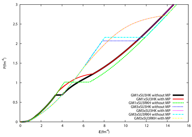
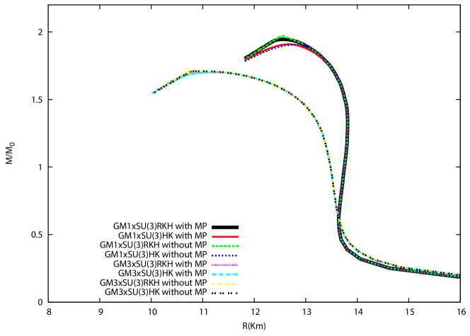
Figure 19: top) EOS built with Maxwell (without MP) and Gibbs (with MP) constructions; bottom) Corresponding mass-radius diagram. Figure based on the results presented in paoli .

A more recent analysis of the dependence of the macroscopic properties of hybrid stars on meson-hyperon coupling constants and on the vector channel added to the NJL model can be seen in Luiz2021 .

In 2019, the LIGO/Virgo collaboration detected yet another gravitational wave, the GW190814 GW190814 , resulting from the merger of a 23 $M_{\odot}$ black hole and another object with $2.59^{+0.08}_{-0.09}M_{\odot}$, which falls in the mass-gap category, i.e., too light to be a black hole and too massive to be a NS. In veronica2 , a chirally invariant model was used to describe hybrid stars with a variety of different vector interactions and this compact object could be explained as a massive rapidly rotating NS. A comprehensive discussion on ultra-heavy NS (masses larger than 2.5 $M_{\odot}$) and the possibility that they are hybrid objects can be found in Veronica_Jacquelyn2021 .

If the reader is interested in understanding the effects of different quark cores that also include trapped neutrinos at fixed entropies, reference trapped can be consulted.

VI Quark stars

All experiments that can be realised in laboratories show that hadrons are the ground state of the strong interaction. Around 50 years ago, Itoh Itoh and Bodmer Bodmer , in separate studies, proposed that under specific circumstances, as the ones existing in the core of neutron stars, strange quark matter (SQM) may be the real ground state. This hypothesis, later on also investigated by Witten, became known as the Bodmer-Witten conjecture and it is theoretically tested with the search of a stability window, defined for different models in such a way that a two- flavour quark matter (2QM) must be unstable (i.e., its energy per baryon has to be larger than 930 MeV, which is the iron binding energy) and SQM (three-flavour quark matter) must be stable, i.e., its energy per baryon must be lower than 930 MeV Bodmer ; Witten . As shown in the previous section, although the Nambu-Jona-Lasinio (NJL) model njl can be used to describe the core of a hybrid star Clebson19 ; DC2003 , it cannot be used in the description of absolutely stable SQM as shown in buballa_stability ; NJLmag ; NJLmag2 ; James_Veronica . The most common model, the MIT bag model mit satisfies the Bodmer-Witten conjecture, but cannot explain massive stars J0348+0432 Antoniadis , J1614-2230 Demorest and J0740+6620) Cromartie ; NICER_news , as can be seen in Fig.20, from where one can observe that the maximum attained mass is 1.94 $M_{\odot}$ obtained for a non-massive strange quark.

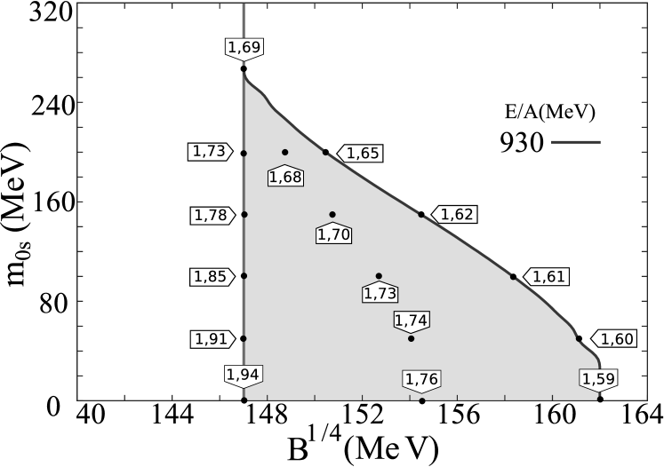
Figure 20: Stability window shown in the shaded area. The flags indicate the maximum stellar masses obtained with various $B$ and strange quark mass values. Figure taken from James2013 .

Hence, we next mention another quark matter model that satisfies de Bodmer-Witten conjecture at the same time that can describe massive stars and canonical stars with small radii, the density dependent quark mass (DDQM) proposed in Peng2000 ; Xia2014 and investigated in Betania21 . In the DDQM model, the quark masses depend on two arbitrary parameters and are given by

$$m_{i}=m_{i0}+m_{I}\equiv m_{i0}+\frac{D}{\rho_{b}^{1/3}}+C\rho_{b}^{1/3},$$ (112)

where the index $I$ stands for the medium corrections and the baryonic density is written in terms of the quark densities as

$$\rho_{b}=\frac{1}{3}\sum_{i}\rho_{i},\quad\rho_{i}=\frac{g_{i}\nu_{i}^{3}}{6\pi^{2}},$$ (113)

and $\nu_{i}$ is the Fermi momentum of quark $i$, which reads:

$$\nu_{i}=\sqrt{\mu_{i}^{*2}-m_{i}^{2}}$$ (114)

and $\mu_{i}^{*}$ is the $i$ quark effective chemical potential. The energy density and pressure are respectively given by

$${\cal E}=\Omega_{0}-\sum_{i}\mu_{i}^{*}\frac{\partial\Omega_{0}}{\partial\mu_{i}^{*}},$$ (115)

and

$$P=-\Omega_{0}+\sum_{i,j}\frac{\partial\Omega_{0}}{\partial m_{j}}n_{i}\frac{\partial m_{j}}{\partial\rho_{i}},$$ (116)

where $\Omega_{0}$ stands for the thermodynamical potential of a free system with particle masses $m_{i}$ and effective chemical potentials $\mu_{i}^{*}$ Peng2000 :

$$\Omega_{0}=-\sum_{i}\frac{g_{i}}{24\pi^{2}}\left[\mu_{i}^{*}\nu_{i}\left(\nu_{i}^{2}-\frac{3}{2}m_{i}^{2}\right)+\frac{3}{2}m_{i}^{4}\ln\frac{\mu_{i}^{*}+\nu_{i}}{m_{i}}\right],$$ (117)

with $g_{i}$ being the degeneracy factor 6 (3 (color) x 2 (spin)) and the relation between the chemical potentials and their effective counterparts is simply

$$\mu_{i}=\mu_{i}^{*}+\frac{1}{3}\frac{\partial m_{I}}{\partial n_{b}}\frac{\partial\Omega_{0}}{\partial m_{I}}\equiv\mu_{i}^{*}-\mu_{I},$$ (118)

On the left of Fig. 21 the stability window is plotted for a fixed value of $C$, so that it displays a shape that can be compared with Fig. 20. For other values of the constants, more stability windows are shown in Betania21 . On the right of Fig. 21, different mass-radius curves are shown and one can see that very massive stars can indeed be obtained. At this point, it is worth mentioning that quark stars are believed to be bare (no crust is supported) and for this reason, the shape of the curves shown in Fig.21 is so different from the ones obtained for hadronic stars and shown in Figs. 11, Fig.12 and for hybrid stars, as seen in Fig.19.

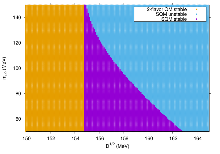
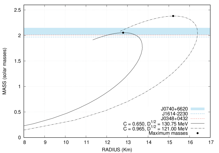
Figure 21: top) Stability window for fixed $C=0$, bottom) Mass-radius diagram for different values of $C$ and $\sqrt{D}$. Figures based on the results shown in Betania21 .

There is still another very promising model, an extension of the MIT bag model based on the ideas of the QHD model. In this extended version, the Lagrangian density accounts for the free Fermi gas part plus a vector interaction and a self-interaction mesonic field and reads Carline1 :

$$\mathcal{L}=\sum_{u,d,s}\{\bar{\psi}_{q}[\gamma^{\mu}(i\partial_{\mu}-g_{qqV}V_{\mu})-m_{q}]\psi_{q}-B\}\Theta(\bar{\psi_{q}}\psi_{q})+\frac{1}{2}m_{\omega}^{2}V_{\mu}V^{\mu}+b_{4}\frac{(g_{uuV}^{2}V_{\mu}V^{\mu})^{2}}{4},$$ (119)

where the quark interaction is mediated by the vector channel $V_{\mu}$ representing the $\omega$ meson, in the same way as in QHD models  walecka . The relative quark-vector field interaction is fixed by symmetry group and results in

$$g_{ssV}=\frac{2}{5}g_{uuV}=\frac{2}{5}g_{ddV},$$ (120)

with adequate redefinitions given by

$$(g_{uuV}/m_{V})^{2}=G_{V},\quad X_{V}=\frac{g_{ssV}}{g_{uuV}}$$ (121)

and $b_{4}$ taken as a free parameter. Using a mean field approximation and solving the Euler-Lagrange equations of motion, the following eigenvalues for the quarks and $V_{0}$ field can be obtained:

$$E_{q}=\mu=\sqrt{m_{q}^{2}+k^{2}}+g_{qqV}V_{0},$$ (122)

$$g_{uuV}V_{0}+\bigg{(}\frac{g_{uuV}}{m_{\omega}}\bigg{)}^{2}\bigg{(}b_{4}(g_{uuV}V_{0})^{3}\bigg{)}=\bigg{(}\frac{g_{uuV}}{m_{\omega}}\bigg{)}\sum_{u,d,s}\bigg{(}\frac{g_{qqV}}{m_{\omega}}\bigg{)}n_{q}.$$

With this new approach, when the self-interaction vector channel is turned off, the stability window increases and a 2.41$M_{\odot}$ quark star that satisfies all astrophysical constraints is obtained. The self-interaction vector channel does not change the stability window, but allow even more flexibility in the calculation of the tidal polarisability and the canonical star radius due to the inclusion of the free parameter $b_{4}$. In this case, a 2.65 $M_{\odot}$ quark star corresponding to a 12.13 km canonical star radius and a tidal polarisability within the expected observed range is obtained along many other results which satisfy many of the presently known astrophysical constraints. Some of the results are displayed in figure 22. After all the discussion on the radii of NS constrained with the help of gravitational wave observation and neutron skin thickness experimental results presented in section IV.2 and on the uncertainty of these values, I just would like to add one comment: contrary to what is obtained for a family of hadronic stars (maximum mass stars are generally associated with a smaller radii than their canonical star counterparts), a family of quark stars may produce canonical stars with radii that can be approximately the same as the maximum mass star radii, depending on the model used Carline1 and this feature could accomodate the recent NICER detections for J0030+0451 and J0740+6620 .

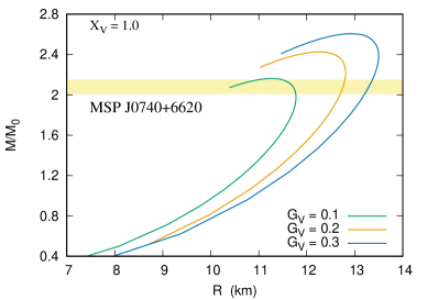
Figure 22: Mass-radius diagram obtained with the minimum value of the bag pressure that produces stable quark stars with different values of $G_{v}$ and top) $X_{v}=0.4$, bottom) $X_{v}=1.0$. Figure based on the results presented in Carline1 .

This modified MIT bag model has also been used to investigate the finite temperature systems and to obtain the QCD phase diagram in Carline2 with the help of a temperature dependent bag $B(T)$, as discussed in the Introduction of the paper. Some of the possible phase diagrams are shown in figure 23.

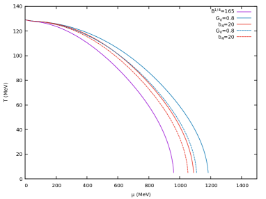
Figure 23: Phase diagram for neutral matter in $\beta$-equilibrium with a temperature dependent bag pressure $B(T)$. Dashed lines stand for $X_{v}=0.4$ and solid lines for $X_{v}=1.0$. Figure based on the results presented in Carline2 .

I have outlined the main aspects concerning the internal structure of quark stars, but the discussion about their bare surface Melrose ; quarkstars is not completely settled Yakovlev and important problems as its high plasma frequency and neutrinosphere are out of the scope of the present work but should not be disregarded.

VII Magnetars: crust-core transitions and oscillations

I could not end this review without mentioning magnetars Duncan ; Pons , a special class of neutron stars with surface magnetic fields three orders of magnitude (reaching up to $10^{15}$ G at the surface) stronger than the ones present in standard neutron stars ($10^{12}$ G at the surface). Most of the known magnetars detected so far are isolated objects, i.e., they are not part of a binary system and manifest themselves as either transient X-ray sources, known as soft-$\gamma$ repeaters or persistent anomalous x-ray pulsars. They are also promising candidates for the recent discovery of fast radio bursts bochenek . So far, only about 30 of them have been clearly identified catalog but more information is expected from NICER NICER and ATHENA ATHENA , launching foreseen to take place in 2030. So far, NICER has already pointed to the fact that the beams of radiation emitted by rapidly rotating pulsars may not be as simple as often supposed: the detection of two hot spots in the same hemisphere suggests a magnetic field configuration more complex than perfectly symmetric dipoles NICER_news .

From the theoretical point of view, there is no reason to believe that the structure of the magnetars differs from the ones I have mentioned in this article. Thus, they can also be described as hadronic objets Lopes2012 ; Rudinei2014 ; Lopes2015 ; Debi2019 ; Lopes2020 ; cesar2020 , as quark stars NJLmag ; Veronica2014 ; Lopes2015 ; Lopes2016 ; Lopes2020 or as hybrid stars Rudinei2014 ; Lopes2020 .

At this point, it is fair to claim that the best approach to calculate macroscopic properties of magnetars is the use of the LORENE code LORENE , which takes into account Einstein-Maxwell equations and equilibrium solutions self consistently with a density dependent magnetic field. LORENE avoids discussions on anisotropic effects and violation of Maxwell equations as pointed out in Lopes2016 , for instance. However, at least two important points involving matter subject to strong magnetic fields can be dealt with even without the LORENE code. The first one is the crust core transition density discussed in Debi2019 and Constanca2017 . Although the magnetic fields at the surface of magnetars are not stronger than $10^{15}$ G, if the crust is as large as expected (about 10% of the size of the star), at the transition region the magnetic field can reach $10^{17}$ G. The transition density can then be estimated by computing the spinodal sections, both dynamically and thermodynamically. The point where the EOS crosses the spinodal defines the transition density older . An interesting aspect is that the spinodals of magnetised matter are no longer smooth curves. Due to the filling of the Landau levels, more than one crossing point is possible Debi2019 ; Constanca2017 , what introduces an extra uncertainty on the calculation.

The second aspect refers to possible oscillations in magnetars caused by the violent dynamics of a merging binary system. One has to bear in mind that so far, all observed magnetars are isolated compact objects, but there is no reason to believe that binary systems do not exist. In this case, the perturbations on the metric can couple to the fluid through the field equations Thorne ; Hinderer . For a comprehensive discussion on the equations involved, please refer to cesar2020 . The gravitational wave frequency of the fundamental mode is expected to be detected in a near future by detectors like the Einstein Telescope. In cesar2020 , the effect of strong magnetic fields on the fundamental mode was investigated. From the results presented in that paper, one can clearly see that magnetars bearing masses below 1.8 M_⊙ present practically the same frequencies. Nevertheless, more massive stars present different frequencies depending on their constitution: nucleonic stars present frequencies lower than their hyperonic counterparts, a feature which may define the internal constitution of magnetars.

The DDQM described in Section VI was also investigated under the effects of strong magnetic fields and the main expressions can be found in Betania_Kauan . This may be an interesting model for future calculations of the fundamental models.

VIII Final Remarks

From the existence of a massive ordinary star that lives due to nuclear fusion, to its explosive ending and its aftermath, I have tried to tell the neutron star history. All these stages can be explained thanks to nuclear physics and I have revisited the main aspects and models underlying each one.

I have also tried to emphasise that nuclear models are generally parameter dependent and a plethora of models have been proposed in the last decades, but it is unlikely that the very same models can be used to describe different aspects of nuclear matter and, at the same time, all macroscopic properties of neutron stars. I do not advocate that the models I have chosen to use are the best ones, but the main idea is to show that different models should be used at the discretion of the people who employ them. I have not used density dependent hadronic models as the ones proposed, for instance, in Typel ; ddme2 to avoid extra theoretical complications, but they are indeed very good options, since they can describe well nuclear matter, finite nuclei and NS properties, as seen in relat ; NS_RMF ; GW_RMF .

As far as detections of gravitational waves are concerned, a window was opened in 2015 and many observations will certainly be disclosed even before I finish writing this paper. Besides the ones already mentioned, I would like to comment on the GW190425 GW190425 , GW200105 and GW200115 GW200115 . The first one was used in conjunction with a chiral effective field theory to constrain the NS equation of state Dietrich2020 . The authors obtained a radius equal to $11.75^{+0.86}_{0.81}$ for a canonical star, also quite small as compared with the ones obtained from the PREX experiment. The other two probably refer to neutron star - black hole mergers, systems that have been conjectured for a long time and will probably contribute to the understanding of NS EOS.

Before concluding, I would like to mention that many aspects regarding either isolated NS or binary systems have not been tackled in this manuscript and, in my opinion, rotation is the most important one. A better understanding of these compact objects depends on many rich features, including thermal and magnetic evolution. Different observation manifestations as pulsars, accreting X-ray binaries, soft $\gamma$-repeaters and anomalous X-ray pulsars, also deserve an attentive investigation. Hence, this review is just one step towards the incredible exotic world of neutron stars.

As far as the QCD phase diagram is concerned, many aspects have been extensively studied and are well understood: matter at zero temperature, symmetric nuclear and pure neutron matter, low density matter, including clusterisation and the pasta phase, high density matter and matter in $\beta$-equilibrium. Nevertheless, an EOS that covers the complete QCD phase diagram parameter space in $(T,\mu_{B})$ in a single model is not available yet. Some of the EOS can be found on the CompOSE (CompStar Online Supernovae Equations of State) website compose .