The Parity Ray Regularizer for Pacing in Auction Markets

Abstract

Budget-management systems are one of the key components of modern auction markets. Internet advertising platforms typically offer advertisers the possibility to pace the rate at which their budget is depleted, through budget-pacing mechanisms. We focus on multiplicative pacing mechanisms in an online setting in which a bidder is repeatedly confronted with a series of advertising opportunities. After collecting bids, each item is then allocated through a single-item, second-price auction. If there were no budgetary constraints, bidding truthfully would be an optimal choice for the advertiser. However, since their budget is limited, the advertiser may want to shade their bid downwards in order to preserve their budget for future opportunities, and to spread expenditures evenly over time. The literature on online pacing problems mostly focuses on the setting in which the bidder optimizes an additive separable objective, such as the total click-through rate or the revenue of the allocation. In many settings, however, bidders may also care about other objectives which oftentimes are non-separable, and therefore not amenable to traditional online learning techniques. Building on recent work, we study the frequent case in which advertisers seek to reach a certain distribution of impressions over a target population of users. We introduce a novel regularizer to achieve this desideratum, and show how to integrate it into an online mirror descent scheme attaining the optimal order of sub-linear regret compared to the optimal allocation in hindsight when inputs are drawn independently, from an unknown distribution. Moreover, we show that our approach can easily be incorporated in standard existing pacing systems that are not usually built for this objective. The effectiveness of our algorithm in internet advertising applications is confirmed by numerical experiments on real-world data.

1 Introduction

In the last decade, the spending on Internet advertising has grown dramatically, reaching more than $130 billion in the United States in 2019 [23]. One of the drivers of this rapid growth has been the success of auction markets as a practical mechanism to match bidders (i.e., advertisers) to their target audience at an appropriate price [22, 40]. In this type of mechanisms, advertisers usually specify a targeting rule to target a certain population of users, and they are asked to bid on events of interest such as an impression, a click, a conversion or a video view. For each ad slot, the mechanism determines a winning advertiser, which is subsequently given the chance to show an impression and potentially generate the event of interest.

Auction markets are typically operationalized through simple mechanisms that can be effectively implemented at scale, and that simplify the interaction between advertisers and the platform. A common paradigm to manage large amounts of repeated ad auctions is for the platform to operate a proxy bidder on behalf of each advertiser. The advertisers communicate the maximum bid for the event of interest, their targeting criteria, and their overall budget for their campaigns to the proxy bidder. In real time, the proxy bidder then constructs bids for each individual auction via these parameters, as well as additional information computed by the platform.

The complexity of the competitive interactions taking place between advertisers, the frequency of the decisions, and the intrinsic uncertainties of the environment make budget management particularly challenging in this setting. An advertiser may lose out on significant amounts of revenue if their budget is depleted too early (thereby missing potentially valuable future bidding opportunities), or if their budget it not fully depleted within the planned duration of the campaign. To solve this problem, platforms offer advertisers the possibility to pace the rate at which their budget is depleted, through a budget-pacing mechanism. The most common pacing mechanisms modify the values of the bids within a series of repeated auctions either by shading the bid appropriately (i.e., multiplicative pacing) [9, 18], or by determining a participation probability through the toss of an appropriately weighted coin for each auction (i.e., probabilistic pacing) [1, 9]. In this work, we focus on the former type of budget-management mechanism. This choice is motivated by the widespread adoption of this mechanisms in large online advertising platforms. Specifically, we study an online setting in which an advertiser is repeatedly confronted with a series of advertising opportunities, one per iteration, allocated through a second-price auction. If there were no budgetary constraints, bidding truthfully (i.e., bidding their true valuation for an advertising opportunity) would be an optimal choice for the advertiser. However, since their budget is limited, the advertiser may want to shade their bid downwards in order to preserve their budget for future opportunities.

The literature on online bidding and online pacing problems mostly focuses on settings in which the bidder optimizes an additively separable objective, such as the total click-through rate or revenue of the allocation (see, e.g., [10, 13, 15, 18, 24, 31]). In many settings, however, advertisers may also care about other objectives which oftentimes are non-separable, and therefore not amenable to traditional online learning techniques. Two notable exceptions are the work by Agrawal and Devanur [2], which focuses on solving general online stochastic convex programs with general concave objectives and convex constraints, and the recent work by Balseiro et al. [12], where the authors study online allocation problems with non-separable objectives in settings such as fairness across advertisers and load balancing. We argue that another frequent objective, which is oftentimes sought after by advertisers, is reaching a certain distribution of impressions over a target population of users. Surprisingly enough, to the best of our knowledge, industry practitioners don’t have at their disposal a practical way to solve this problem. Consider, for example, the following real-world use cases: an advertiser may want to enforce uniform sampling on a target population for conducting unbiased surveys, to promote a business based on a two-sided market by balancing their reach on users belonging to “both sides of the market” (this is the case, for example, of dating apps, and online marketplaces), or to perform online outreach to a population of users. In the latter setting, Gelauff et al. [28] showed that advertisers have to resort to complex segmentation strategies through subcampaigns to achieve a distribution of conversions close to that of the overall adult population of a target city.

Our contributions

Thus motivated, we present a practical way to steer a multiplicative-pacing mechanism so as to satisfy advertisers’ distributional preferences over the advertising opportunities which they are allocated. In particular, an advertiser may want to reach a realized distribution of impressions close to some target distribution across a given user breakdown. We refer to the feature determining the breakdown of interest as the category of the user. We consider a finite horizon model in which an advertiser participates in a series of auctions. The advertiser has a fixed amount of non-replenishable resources (i.e., a budget). We consider an incomplete information model where, at each iteration, an item is drawn i.i.d. from some unknown distribution and presented to the advertiser, who has to compute a bid for the current item. Then, a second-price auction is run and the advertiser observes their reward and budget consumption. The advertiser does not get to observe the reward functions and types of future requests until their arrival. First, we describe a regularizer, which we call the parity ray regularizer, that can be employed to model the advertiser’s distributional preferences. Second, we propose a practical mechanism for our specific regularized online pacing problem by casting the online mirror descent scheme by Balseiro et al. [12] to our setting. Our algorithm guarantees regret of order $O(T^{1/2})$, which optimal in our stochastic setting. Moreover, we show that our framework could easily be incorporated into standard existing pacing systems that are not usually built for this objective. Finally, we empirically demonstrate the efficacy of our mechanism on real-world data from a large Internet advertising company.

2 Multiplicative pacing for auction markets

We study the problem faced by a bidder (i.e., an advertiser) who wishes to maximize their utility over a sequence of auctions that occur over $T$ time steps. At each time $t=1,\ldots,T$ an item (i.e., an advertising opportunity to reach a user) appears, and an auction is run in order to allocate it. We will assume that the item is allocated via a single-item second-price auction, meaning that the highest bid wins, and the winner pays the second-highest bid. At every time $t$, the bidder observes their valuation $v_{t}$ for the item, submits a bid $b_{t}$, and then observes the variable $x_{t}\in\{0,1\}$ specifying whether they won, and if they did win then they observe the price $p_{t}$ that they paid for the item.

Without further restrictions, bidding in such a dynamic auction setting would be straightforward: the bidder can simply bid their true value, and the second-price auction ensures that this maximizes their utility. However, in practice, bidders usually have a total budget $B$, and they wish to constrain their expenditure across the $T$ auctions to be at most $B$. This complicates bidding even in second-price auctions, because this budget constraint links all $T$ auctions together. If we allow fractional allocations, then an omniscient budget-constrained bidder can be thought of as a fractional knapsack packer: they now wish to order the $T$ auctions by decreasing bang-per-buck $v_{t}/p_{t}$, and grab items in this order until they either deplete their budget, or they reach some item $t$ such that $v_{t}/p_{t}\leq 1$ [18]. In practice, the bidder must decide their bids in an online fashion: at time $t$ they only know their first $t$ valuations $(v_{1},\ldots,v_{t})$, their past allocations up to time $t-1$, i.e., $(x_{1},\ldots x_{t-1})$, as well as their past expenditures $(x_{1}p_{1},\ldots,x_{t-1}p_{t-1})$. Thus, the only information they have about the auction at time $t$ is their valuation for the item, and they must adaptively smooth out their spending across the $T$ auctions, in order to satisfy their budget constraint while maximizing utility.

The above problem of how to bid in such a setting has been studied extensively both from the perspective of an individual bidder, as well as from a platform perspective. One popular approach in practice is to use a pacing multiplier $\alpha\in[0,1]$, which is then used to construct each bid as $b_{t}=\alpha v_{t}$. Given a sequence of prices $(p_{1},\ldots,p_{T})$, an optimal allocation can be achieved within the context of second-price auctions by choosing $\alpha$ such that the bidder spends their budget exactly (assuming that the bidder can choose the fraction that they wish to win on any items such that $\alpha v_{t}=p_{t}$) [14, 18]. The pacing multiplier can be adaptively controlled via online-learning methods in order to guarantee asymptotic optimality in stochastic environments [13, 10].

In the above, we presented the setting as if the individual bidder controls their pacing parameter $\alpha$ used in smoothing their expenditure. However, a second model which arises in practice is the proxy-bidder setting. The proxy-bidder setting arises in online advertising, where advertisers often submit only a value per click, budget, and targeting criteria to the platform. The platform then performs budget smoothing on behalf of the advertiser. In that setting, the proxy bidder refers to a bidder operated by the platform, which is effectively a control algorithm that scales the parameter $\alpha$ up or down, depending on whether the advertiser is on track to spend their budget correctly across the given time frame. Equilibria arising in the proxy-bidder setting have been studied in several works (see, e.g., [9, 18, 17]).

3 Problem description

In this paper, we focus on the setting where we wish to smooth out the expenditure of a single bidder, while the rest of the market behaves according to a stochastic model. In particular, we will assume that valuations, prices, and user categories are generated i.i.d. from an unknown distribution. In practice, valuations and categories can be safely described as coming from a stochastic model. The prices, however, typically come from the paced bids arising from other bidders whom are also employing some budget-smoothing technique. In small-scale settings where bidders react to the expenditure of other bidders, these prices could behave adversarially rather than stochastically. However, for large-scale markets, an individual bidder has almost no impact on the prices or the overall market, in which case stochastic behavior of the prices is a reasonable assumption. This idea can be formalized, for example, via fluid mean-field models such as the one given by Balseiro et al. [14].

The bidder can spend a budget $B$ over a sequence of auctions withing a finite time horizon $T$. Let $\bm{x}\in[0,1]^{T}$ be the allocation vector for the bidder, and $x_{t}\in\mathcal{X}_{t}\subseteq[0,1]$ be the allocation at time $t$. Let $\rho\in\mathbb{R}_{>0}$ be the per-iteration budget, which is a constant such that $B=T\rho$. Items can be of $m$ different types or, equivalently, categories. The vector $\bm{c}_{t}\in[0,1]^{m}$ specifies the categories of the item being auctioned at time $t$. At each iteration $t$, the bidder receives as input the tuple $(v_{t},p_{t},\bm{c}_{t})$ specifying the valuation for the item $v_{t}\in\mathbb{R}_{\geq 0}$, its price $p_{t}\in\mathbb{R}_{\geq 0}$, and its category vector $\bm{c}_{t}$. At each $t$, the input tuple is generated i.i.d. from an unknown distribution $\mathscr{P}\in\Delta^{\mathcal{I}}$, where $\mathcal{I}$ is the set of all possible input tuples that can be observed. In the remainder of the paper we make the following assumption on the regularity of inputs, which is easily satisfied in practice.

Assumption 1.

There exists $\bar{v}\in\mathbb{R}_{\geq 0}$ and $\bar{p}\in\mathbb{R}_{\geq 0}$ such that, for any input tuple $(v_{t},p_{t},\bm{c}_{t})\in\mathcal{I}$ in the support of $\mathscr{P}$, it holds $v_{t}\leq\bar{v}$ and $p_{t}\leq\bar{p}$.

Let $f_{t}:[0,1]\to\mathbb{R}$ be the reward function at time $t$ such that, for each $x\in\mathcal{X}_{t}$,

$$f_{t}(x)\mathrel{:\mkern-0.25mu=}(v_{t}-p_{t})x.$$ (1)

Then, given a generic concave regularizer $R:\mathbb{R}_{\geq 0}^{m}\to\mathbb{R}$, we are interested in finding an online algorithm guaranteeing performance close to that of the optimal solution in hindsight, which we denote by $\textsc{Opt}(\mathscr{P})$. In particular, this baseline is the expected reward that the bidder would achieve by computing the optimal allocation $\bm{x}$ when the input sequence from $t=1$ to $T$ is known in advance. Computing $\textsc{Opt}(\mathscr{P})$ amounts to solving the offline optimal allocation problem for each possible realized input sequence, and by taking expectations according to the realization probability specified by $\mathscr{P}$. Formally, it is defined as follows

$$\textsc{Opt}(\mathscr{P})\mathrel{:\mkern-0.25mu=}\mathbb{E}_{\mathscr{P}}\left[\begin{array}[]{l}\displaystyle\max_{\bm{x}:x_{t}\in\mathcal{X}_{t}}\sum_{t=1}^{T}f_{t}(x_{t})+TR\left(\frac{1}{T}\sum_{t=1}^{T}\bm{c}_{t}x_{t}\right)\\[5.69054pt] \displaystyle\text{s.t. }\sum_{t=1}^{T}p_{t}x_{t}\leq T\rho\end{array}\right].$$ (2)

4 Parity ray regularizer

For simplicity, we assume that a type specifies a convex combination over categories, that is, for any $t$, the vector of realized categories $\bm{c}_{t}$ belongs to $\mathcal{C}\mathrel{:\mkern-0.25mu=}\left\{\bm{c}\in[0,1]^{m}:\sum_{i}c_{i}=1\right\}$. This assumption can be relaxed to a larger bounded set. Given a target distribution over categories $\hat{\bm{x}}\in\Delta^{m}$, we consider a setting where the bidder is interested in steering their realized distribution of impressions towards $\hat{\bm{x}}$. Given a time horizon $T$, a sequence of types $(\bm{c}_{t})_{t=1}^{T}$, and $\hat{\bm{x}}\in\Delta^{m}$, the bidder’s goal is to obtain a vector of allocations $\bm{x}\in[0,1]^{T}$ such that, for each $i\in[m]$, $\sum_{t=1}^{T}c_{t,i}x_{t}/\sum_{t=1}^{T}x_{t}$ is close to $\hat{x}_{i}$. However, directly handling such realized distribution of impressions entails solving a non-convex optimization problem. Then, a natural question is the following: is it possible to incorporate such distributional preference as a concave regularization term in the bidder’s objective function?

We propose the following regularization term as a natural solution for this problem.

Definition 1 (Parity ray regularizer).

Let $D:\Delta^{m}_{+}\times\Delta^{m}_{+}\to\mathbb{R}_{\geq 0}$. Then, given a target distribution $\hat{\bm{x}}\in\Delta^{m}$, the parity ray regularizer is a function $R:\Delta^{m}_{+}\times\Delta^{m}_{+}\to\mathbb{R}_{\leq 0}$ such that, for any vector $\bar{\bm{x}}\in\Delta^{m}_{+}$, it holds

$$R(\bar{\bm{x}})\mathrel{:\mkern-0.25mu=}-\min_{\gamma\in[0,1]}D\left(\gamma\hat{\bm{x}};\bar{\bm{x}}\right).$$

We say that a bidder is optimizing for their parity-regularized utility if they are solving Problem (2) and $R$ is defined as in Definition 1. Intuitively, $D$ acts as a pseudo-distance measure on $\Delta^{m}_{+}$. It is not a true distance metric because we will not be assuming that it satisfies all the conditions of a metric. It can be thought of as analogous to a divergence from statistics, although we measure distances on the full-dimensional simplex. Given some current distribution $\bar{\bm{x}}$, $R$ performs a projection onto the line segment generated by $[0,1]\times\hat{\bm{x}}$, where the projection is in terms of $D$ (this is analogous to, e.g., a Bregman projection).

The “parity ray” name comes from the fact that we can think of $R$ as measuring the distance between a given point $\bar{\bm{x}}\in\Delta^{m}_{+}$ to the ray $\{\gamma\hat{\bm{x}}:\gamma\geq 0\}$. In our definition we only consider a segment of this ray by restricting $\gamma\in[0,1]$. This restriction is mostly for analytical convenience when deriving Lipschitz constants below. For a suitable $D$ that extends to the positive orthant, one could remove the restriction and measure distances on the whole positive orthant.

We will assume that $D$ satisfies a number of properties that will allow us to optimize it as part of an online optimization procedure.

Assumption 2.

We assume that $D(\bar{\bm{x}};\bm{x})$ satisfies the following conditions:

• $D$ is jointly convex on $\Delta^{m}_{+}\times\Delta^{m}_{+}$, and $D(\bm{x};\bar{\bm{x}})\in[0,\bar{r}]$ for all $\bm{x},\bar{\bm{x}}\in\Delta^{m}_{+}$.

• For a fixed $\gamma$, the function $D(\gamma\hat{\bm{x}};\cdot)$ is $L$-Lipschitz with respect to the second argument under some $\ell_{p}$ norm.

Proposition 1.

Given 2, the regularizer $R$ is concave, closed, and for each $\bm{x}\in\Delta_{+}^{m}$, $R(\bm{x})\in[\underline{r},0]$ with $\underline{r}=-\bar{r}$. Furthermore, $R$ is $L$-Lipschitz continuous under the $\ell_{p}$ norm.

For any $\ell_{p}$ norm, the distance $D_{p}(\bm{x};\bar{\bm{x}})=\|\bm{x}-\bar{\bm{x}}\|_{p}$ satisfies 2. In particular, $D_{p}$ is $1$ Lipschitz with respect to $\ell_{p}$, and the remaining properties follow directly from the definition of a norm and the fact that $D_{p}$ is defined on a bounded set $\Delta^{m}_{+}$. Moreover, the $\ell_{2}$ norm yields a simple closed form solution for the parity ray regularizer, which is particularly appealing for practical purposes. In particular, we have that for any $\bar{\bm{x}}\in\Delta_{+}^{m}$, $R(\bar{\bm{x}})=-\|\bar{\bm{x}}-\left(\langle\bar{\bm{x}},\hat{\bm{x}}\rangle/\|\hat{\bm{x}}\|_{2}^{2}\right)\hat{\bm{x}}\|_{2}$, which is well defined with respect to Definition 1 since $0\leq\langle\bar{\bm{x}},\hat{\bm{x}}\rangle/\|\hat{\bm{x}}\|_{2}^{2}\leq 1$.

Another source of appropriate choices for $D$ are $f$-divergences: $D_{f}(\bm{x};\bar{\bm{x}})=\sum_{i=1}^{m}\bar{\bm{x}}_{i}f(\bm{x}_{i}/\bar{\bm{x}}_{i})$ defined with respect to some convex function $f$, since $f$-divergences are jointly convex. However, $f$-divergences are not necessarily $L$ Lipschitz for a fixed $L$. In the case where we wish to use a non-Lipschitz $f$, we have to modify $f$ such that $|\frac{s}{t^{2}}f^{\prime}(s/t)|\leq L$ for $s,t\in[0,1]$. For example, setting $f(t)=t\log t$ yields the Kullback-Leibler (KL) divergence. However, we need to slightly modify the KL divergence in order to ensure that 2 is satisfied: (1) we must shift if by $\log m$ to make it nonnegative, and (2) we make it Lipschitz in the second argument by setting $f(t)=t\log\min(t,1/\epsilon)$; $\epsilon$ then more-or-less corresponds to a lower probability threshold at which we stop increasing the penalty. This lower threshold may actually be useful in practice, to prevent the algorithm from reacting too aggressively to allocation imbalances at the first few iterations.

5 Online allocation algorithm

First, we show that a suitably defined Lagrangian dual function provides an upper bound on $\textsc{Opt}(\mathscr{P})$ (omitted proofs are reported in Appendix B). Let $f^{\ast}_{t}:\mathbb{R}_{\geq 0}\to\mathbb{R}$ be the conjugate function of $f_{t}$ as defined in Equation 1 restricted to $\mathcal{X}_{t}$, that is, for all $\mu\in\mathbb{R}_{\geq 0}$,

$$f^{\ast}_{t}(\mu)\mathrel{:\mkern-0.25mu=}\sup_{x\in\mathcal{X}^{t}}\left\{f_{t}(x)-\mu x\right\}.$$

Moreover, let $R^{\ast}:\mathbb{R}^{m}\to\mathbb{R}$ be the conjugate function of the regularizer $R$ restricted to $\Delta_{+}^{m}$. Formally, for each $\bm{\lambda}\in\mathbb{R}^{m}$,

$$R^{\ast}(-\bm{\lambda})\mathrel{:\mkern-0.25mu=}\sup_{\bar{\bm{x}}\in\Delta^{m}_{+}}\left\{R(\bar{\bm{x}})+\langle\bm{\lambda},\bar{\bm{x}}\rangle\right\}.$$

Let $\mathcal{D}$ be the set of dual variables for which the conjugate of the regularizer is bounded. Formally,

Lemma 1.

$\mathcal{D}\mathrel{:\mkern-0.25mu=}\left\{(\mu,\bm{\lambda})\in\mathbb{R}_{\geq 0}\times\mathbb{R}^{m}:-\infty<R^{\ast}(-\bm{\lambda})<+\infty\right\}=\mathbb{R}_{\geq 0}\times\mathbb{R}^{m}$.

For a given distribution $\mathscr{P}$ over the finite set of possible input tuples $\mathcal{I}$, the Lagrangian dual function $D(\mu,\bm{\lambda}|\mathscr{P}):\mathcal{D}\to\mathbb{R}$ is such that, for each pair of dual variables $(\mu,\bm{\lambda})\in\mathcal{D}$,

$$D(\mu,\bm{\lambda}|\mathscr{P})\mathrel{:\mkern-0.25mu=}\mathbb{E}_{(v_{t},p_{t},\bm{c}_{t})\sim\mathscr{P}}\left[f^{\ast}_{t}\left(\mu p_{t}+\langle\bm{\lambda},\bm{c}_{t}\rangle\right)+R^{\ast}(-\bm{\lambda})\right]+\rho\mu.$$ (3)

Then, the following holds.

Theorem 1.

Given a time horizon $T\geq 0$, for any $(\mu,\bm{\lambda})\in\mathcal{D}$, $\textsc{Opt}(\mathscr{P})\leq TD(\mu,\bm{\lambda}|\mathscr{P})$.

Given this intermediate result, we describe an online allocation algorithm (Algorithm 1) based on the online mirror descent scheme by Balseiro et al. [10], which we adapt to account for parity-regularized objectives (which are non-separable). We exploit the specific structure of our problem to recover better constants in the regret upper bound (see Theorem 2), and to relax some of the assumptions required by Balseiro et al. [10] (see 2). For a specific choice of the reference function $\psi$, Algorithm 1 gives an instantiation of the dual subgradient descent algorithm by Balseiro et al. [12] for our setting. Therefore, the dual subgradient descent algorithm by Balseiro et al. [12] is a special case of Algorithm 1.

The algorithm proceeds according to the following main steps:

Primal decision

At each time step $t$, given input tuple $(v_{t},p_{c},\bm{c}_{t})$, the algorithm computes the optimal allocation $\hat{x}$ which maximizes an opportunity cost-adjusted reward, based on the current dual solutions $(\mu_{t},\bm{\lambda}_{t})$ (Equation 4). The optimal decision $\hat{x}$ is taken if the remaining budget is enough to cover costs, that is, $p_{t}\hat{x}\leq B_{t}$. Finally, the target distribution over categories $\bar{\bm{x}}_{t}$ is computed by computing the value maximizing the regularizer $R$ adjusted by an additive term accounting for the current dual solution $\bm{\lambda}_{t}$ (Equation 5).

Dual variables update

First, the algorithm computes an unbiased stochastic estimator of a subgradient of $D(\mu,\bm{\lambda}|\mathscr{P})$ at $(\mu_{t},\bm{\lambda}_{t})$ (Equation 6). The algorithm employs this estimator to update the vector of dual variables by performing an online dual mirror descent descent step with step size $\eta$ and reference function $\psi$ (Equation 7).

Intuitively, at each time step $t$, the algorithm compares (i) the actual expenditure from the auction to the expected rate of spend per iteration $\rho$, and (ii) the target distribution over categories at $t$ to the realized category. If the actual expenditure is higher (resp., lower) than this expected rate, then the algorithm surmises that future opportunities will offer higher (resp., lower) bang for the buck than current opportunities, and therefore the algorithm lowers (resp., raises) the bid shading multiplier. At the same time, if the realized category causes an undesired skew, and moves the realized distribution of impressions away from the desired $\bar{\bm{x}}_{t}$, then the algorithm will adjust its dual solutions to penalize allocations from that category, and increase the likelihood of acceptance for items coming from under-represented categories.

Input: Initial dual solutions $(\mu_{1},\bm{\lambda}_{1})$, time horizon $T$, initial budget consumption $B_{1}=B$, function $\psi$, step-size $\eta$.

for $t=1,\ldots,T$ do

       Observe $(v_{t},p_{t},\bm{c}_{t})\sim\mathscr{P}$

       Compute primal decision:

      

$$\hat{x}\in\operatorname*{arg\,max}_{x\in\mathcal{X}_{t}}\left\{f_{t}(x)-\mu_{t}p_{t}x-\langle\bm{\lambda}_{t},\bm{c}_{t}\,\,x\rangle\right\}$$ (4)

      

$$x_{t}=\left\{\begin{array}[]{l}\hat{x}\hskip 8.5359pt\text{if }p_{t}\hat{x}\leq B_{t}\\[5.69054pt] 0\hskip 11.38092pt\text{otherwise}\end{array}\right.$$

      

$$\bar{\bm{x}}_{t}\in\operatorname*{arg\,max}_{\bar{\bm{x}}^{\prime}\in\Delta_{+}^{m}}\left\{R(\bar{\bm{x}}^{\prime})+\langle\bm{\lambda}_{t},\bar{\bm{x}}^{\prime}\rangle\right\}$$ (5)

       Update resource consumption: $B_{t+1}=B_{t}-p_{t}x_{t}$

       Compute subgradient $\bm{g}\in\mathbb{R}^{m+1}$ of $D(\mu_{t},\bm{\lambda}_{t}|\mathscr{P})$:

      

$$\bm{g}=\left(\rho-p_{t}\hat{x},\,\,\bar{\bm{x}}_{t}-\bm{c}_{t}\hat{x}\right)$$ (6)

       Update dual variables:

      

$$(\mu_{t+1},\bm{\lambda}_{t+1})=\operatorname*{arg\,min}_{(\mu,\bm{\lambda})\in\mathcal{D}}\left\{\langle\bm{g},(\mu,\bm{\lambda})\rangle+\frac{1}{\eta}B_{\psi}((\mu,\bm{\lambda}),(\mu_{t},\bm{\lambda}_{t}))\right\}$$ (7)

end for

Algorithm 1 Online allocation algorithm for parity-regularized pacing

5.1 Regret bound

We focus on the stochastic setting in which, at each $t$, an input tuple is drawn i.i.d. from $\mathscr{P}$. This setting is particularly relevant for applications to large Internet advertising platforms in which the number of bidders interacting makes the environment unlikely to react adversarially to choices of one specific bidder. We show that Algorithm 1 attains a sublinear regret of order $O(T^{1/2})$.

Let $\tau$ be the time at which the budget of the bidder is depleted when following Algorithm 1. By playing according to Algorithm 1, the bidder attains the following expected reward:

$$\textsc{Rew}(\mathscr{P})\mathrel{:\mkern-0.25mu=}\mathbb{E}_{\mathscr{P}}\left[\sum_{t=1}^{T}f_{t}(x_{t})+TR\left(\frac{1}{T}\sum_{t=1}^{T}\bm{c}_{t}x_{t}\right)\right].$$ (8)

We start with the following intermediate result which provides a lower bound on the expected reward attained by following Algorithm 1 up to the time $\tau$ in which the budget is fully depleted.

Lemma 2.

Consider an arbitrary $\mathscr{P}\in\Delta^{\mathcal{I}}$. For each $t\in[T]$, let $x_{t}$ and $\bar{x}_{t}$ be computed according to Equation 4 and Equation 5, respectively. Moreover, given the time of budget depletion $\tau$, let

$$\bar{\mu}=\frac{1}{\tau}\sum_{t=1}^{\tau}\mu_{t}\quad\text{and }\quad\bar{\bm{\lambda}}=\frac{1}{\tau}\sum_{t=1}^{\tau}\bm{\lambda}_{t}.$$

Then, it holds

$$\mathbb{E}_{\mathscr{P}}\left[\sum_{t=1}^{\tau}\left(f_{t}(x_{t})+R(\bar{\bm{x}}_{t})\right)\right]\geq\mathbb{E}_{\mathscr{P}}\left[\tau D(\bar{\mu},\bar{\bm{\lambda}}|\mathscr{P})-\sum_{t=1}^{\tau}\left(\mu_{t}(\rho-p_{t}x_{t})-\langle\bm{\lambda}_{t},\bar{\bm{x}}_{t}-\bm{c}_{t}x_{t}\rangle\right)\right].$$

In order to prove the regret bound of Theorem 2 we need the following additional assumption on the reference function $\psi$ of the Bregman divergence $B_{\psi}$.

Assumption 3.

The reference function $\psi$ is $\sigma$-strongly convex with respect to an $\ell_{p}$ norm $\left\lVert\cdot\right\rVert_{p}$.

This assumption is a relaxation of the requirements in Balseiro et al. [10, Assumption 2] (i.e., strong convexity with respect to $\|\cdot\|_{1}$). Indeed, by exploiting the specific structure of our problem, we can prove the following.

Theorem 2.

Consider Algorithm 1 with step-size $\eta\geq 0$ and initial solution $(\mu_{1},\bm{\lambda}_{1})\in\mathcal{D}$. Suppose 1, Proposition 1, and 3 are satisfied, and the requests are drawn i.i.d. from an unknown distribution $\mathscr{P}\in\Delta^{\mathcal{I}}$. Then, for any $T\geq 1$, it holds

$$\textsc{Opt}(\mathscr{P})-\textsc{Rew}(\mathscr{P})\leq C_{1}+\frac{G^{2}\eta}{\sigma}T+\frac{1}{\eta}C_{2},$$

where $C_{1}=(\bar{v}-\underline{r}+2L)\bar{p}/\rho$, $G=\max\{\rho+\bar{p},2\}$, and

$$C_{2}=2\sup\{B_{\psi}((\mu,\bm{\lambda}),\bm{d}_{1}):(\mu,\bm{\lambda})\in\mathcal{D},\left\lVert\bm{\lambda}\right\rVert\leq L\}.$$

By setting $\eta\sim T^{-1/2}$ we obtain a regret of order $O(T^{1/2})$, which is the optimal order of regret that can be attained in this setting as shown by Arlotto and Gurvich [6, Lemma 1].

6 Regularized pacing within a paced-auction framework

One of the major selling points of our approach to enforcing distributional preferences via regularization is that Algorithm 1 can easily be incorporated in existing pacing systems that are not necessarily built around this objective. In Section 2 we described how pacing systems with proxy bidders work for large-scale Internet advertising. In that setup, the platform controls a proxy bidder on behalf of every advertiser $i$, where the proxy bidder uses a control algorithm on the pacing parameter $\alpha_{i}$ used to construct bids, in order to ensure that the advertiser satisfies their budget constraint. An important feature of this setup is that each proxy bidder can control their own pacing parameter $\alpha_{i}$ purely through their observed spending. This leads to a highly decentralized framework, where communication between proxy bidders is only necessary via the second-price auctions that sell items whenever they show up, and bidders only need to submit their paced bids to these auctions. This decentralization is important, because centralized optimization problems may not be realistic to solve every time a user shows up on the site. In the remainder of the section we explain how a bidder may implement our Algorithm 1 via a form of decentralized double-pacing. We do this to explain it in generality, but we emphasize that the proxy-bidder setting is one of our main motivations.

Consider a bidder who attempts to maximize parity-regularized utility. By using Algorithm 1, the bidder will have two parameters at time $t$: $\mu_{t}$ and $\bm{\lambda}_{t}$, with some item of value $v_{t}$ having appeared (the price $p_{t}$ would not be known yet since the auction has not been run). Algorithm 1 requires that the bidder achieve an allocation that solves Equation 4, which we can rewrite as follows:

$$\operatorname*{arg\,max}_{x\in\{0,1\}}\left\{f_{t}(x)-\mu_{t}p_{t}x-\langle\bm{\lambda}_{t},\bm{c}_{t}x\rangle\right\} =\operatorname*{arg\,max}_{x\in\{0,1\}}\left\{v_{t}x-(1+\mu_{t})p_{t}x-\langle\bm{\lambda}_{t},\bm{c}_{t}\rangle x\right\}$$

$$=\operatorname*{arg\,max}_{x\in\{0,1\}}\left\{(v_{t}-\langle\bm{\lambda}_{t},\bm{c}_{t}\rangle)x-(1+\mu_{t})p_{t}x\right\}$$

$$=\operatorname*{arg\,max}_{x\in\{0,1\}}\left\{\frac{v_{t}-\langle\bm{\lambda}_{t},\bm{c}_{t}\rangle}{1+\mu_{t}}x-p_{t}x\right\}.$$

From the above derivations, we observe at each $t$ that there are three possible cases: (i) the bidder needs to win the item at time $t$ if $\frac{v_{t}-\langle\bm{\lambda}_{t},\bm{c}_{t}\rangle}{1+\mu_{t}}>p_{t}$; (ii) the bidder has to pass on the item if the strict inequality is reversed; (iii) the bidder is indifferent if equality holds. Even though the bidder does not know $p_{t}$, this is exactly achieved within a second-price auction framework by bidding the value $\frac{v_{t}-\langle\bm{\lambda}_{t},\bm{c}_{t}\rangle}{1+\mu_{t}}$ at time $t$. Here, $1/(1+\mu_{t})$ plays the role of the standard multiplicative pacing parameter, but before multiplicative pacing, the bidder first applies an additive pacing term $\langle\bm{\lambda}_{t},\bm{c}_{t}\rangle$.

Thus, we see that our approach can easily be adopted by individual bidders that wish to incorporate distributional regularization as part of their bidding procedure in a repeated-auction setting. For the same reason, proxy bidders can easily incorporate this in the case where an advertising platform wishes to enforce some amount of distributional parity while performing budget-pacing on behalf of the advertisers.

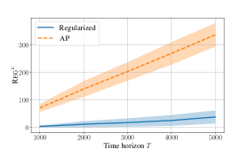
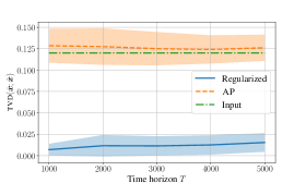
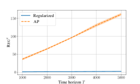
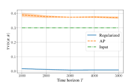
Figure 1: (Top-Left): Empirical upper bound on the regret (i.e., $\textsc{Reg}^{\textsc{u}}$ as defined in Equation 9) for breakdown B2. (Top-Right): Total variation distance from the target distribution $\hat{\bm{x}}$ for B2. (Bottom-Left): Empirical upper bound on the regret for breakdown B3. (Bottom-Right): Total variation distance from the target distribution $\hat{\bm{x}}$ for B3. Input denotes the total variation distance between $\hat{\bm{x}}$ and the underlying empirical category distribution computed on the dataset.

7 Experimental evaluation

In this section, we present numerical experiments on data from a large Internet advertising company.

Experimental setup

We construct a real-world dataset through logs of a large Internet advertising company. In this dataset, we have one advertiser (more specifically, we consider data at individual campaign level) participating in a sequence of auctions. We consider only ad requests coming from mobile devices. For each ad request we retrieve the advertiser’s bid, the price computed via the auction mechanism, and the relevant categories for the request. We observe that, due to the nature of the bidding system, the bids provide a good approximation to the true advertiser’s valuations. Bids and prices are suitably normalized for privacy reasons. Then, we generate a dataset consisting of $10^{6}$ entries (i.e., one entry per ad requests) and, at each run of the algorithm, we sample from this dataset $T$ requests without replacement. We consider two different ad-request breakdowns. The first one, denoted as breakdown B2, is a binary breakdown (i.e., $m=2$) where the category is the type of mobile device originating the request (we consider the two most frequent such types). The second one, which we denote by B3, is a breakdown into three categories (i.e., $m=3$) determined by the manufacturer of the mobile device. In all of the experiments we set $\rho$ to be approximately equal to the $0.5$ quantile of the empirical distribution of normalized prices from our dataset. In this way, the advertiser is set to win at most half of the ad requests which they are presented.

Algorithms

We instantiate parity ray regularizers with $D_{2}(\bm{x};\bar{\bm{x}})=\|\bm{x}-\bar{\bm{x}}\|_{2}$ as the pseudo-distance measure. Moreover, given a sequence of input tuples $(v_{t},p_{t},\bm{c}_{t})_{t=1}^{T}$, let

$$\textsc{Opt}^{\textsc{u}}\left((v_{t},p_{t},\bm{c}_{t})_{t=1}^{T}\right)\mathrel{:\mkern-0.25mu=}\max_{\bm{x}:x_{t}\in\mathcal{X}_{t}}\sum_{t=1}^{T}f_{t}(x_{t})\,\,\text{s.t. }\,\sum_{t=1}^{T}p_{t}x_{t}\leq T\rho$$

be the value of an optimal allocation in absence of regularization penalties. Then, we evaluate the regret guarantees of our algorithm by computing an upper bound to the parity-regularized regret $\textsc{Opt}(\mathscr{P})-\textsc{Rew}(\mathscr{P})$. In particular, we compute

$$\textsc{Reg}^{\textsc{u}}\left((x_{t},v_{t},p_{t},\bm{c}_{t})_{t=1}^{T}\right)\mathrel{:\mkern-0.25mu=}\textsc{Opt}^{\textsc{u}}\left((v_{t},p_{t},\bm{c}_{t})_{t=1}^{T}\right)-\textsc{Rew}\left((x_{t},v_{t},p_{t},\bm{c}_{t})_{t=1}^{T}\right),$$ (9)

where $\textsc{Rew}\left((x_{t},v_{t},p_{t},\bm{c}_{t})_{t=1}^{T}\right)$ is the realized reward for the sequence of online decisions $\bm{x}$. The baseline algorithm which we employ is the adaptive pacing algorithm (AP) by Balseiro and Gur [13], which guarantees optimal regret in the stochastic setting without regularization. The step size is $\eta=0.1/\sqrt{T}$. This choice guarantees the optimal order of regret both for our algorithm, and for adaptive pacing (in the non-reqularized setting). Dual variables are initialized to $0$. Convex programs are solved using the Xpress Optimization Suite 8.10 [27]. All experiments are run on a 24-core machine with 57 GB of RAM.

Results

We run $20$ independent trials for each time horizon $T\in\{10^{3},2\cdot 10^{3},\ldots,5\cdot 10^{3}\}$. The left column of Figure 1 reports the empirical upper bounds on the regret computed as in Equation 9. The right column of Figure 1 reports the total variation distance between the realized distributions of impressions $\bar{\bm{x}}$ and the target distribution $\hat{\bm{x}}$. We compute this distance as $\textsc{tvd}(\bar{\bm{x}};\hat{\bm{x}})=\sup_{j}|\bar{x}_{j}-\hat{x}_{j}|$. The first row of Figure 1 reports result for the B2 breakdown. In this setting, we set $\hat{\bm{x}}=(.5,.5)$, that is, the advertiser seeks to reach a uniform realized distribution of impressions over the two mobile device types. Algorithm 1 achieves small regret over all time horizons, and guarantees a realized distribution of impression close to the target. On the other hand, the adaptive pacing algorithm shows linear regret in $T$, which is due to the penalty for not being able to steer the realized distribution of impression towards the target. The same behavior can be observed in the B3 setting. Here, the empirical distribution of categories of the dataset is roughly $(.5,.3,.2)$. To make the problem harder, we try to skew the realized distribution of impressions towards the least frequent category by setting $\hat{\bm{x}}=(.1,.3,.6)$. Algorithm 1 manages to keep the resulting distribution close to the target even in this challenging setting. It is interesting to notice that the distribution over categories of the input data would be closer to the target distribution than what achieved by the adaptive pacing algorithm. The same behavior can be observed when we artificially create an unbalance between the distribution of prices for the different categories. In these extreme cases, the adaptive pacing algorithm forces the advertiser to win only impression of the cheap category (see Appendix C).

Appendix A Related works

Online allocation problems have been studied from a number of different perspectives. One stream of works addresses the case in which inputs are chosen by an adversary (see, e.g., Mehta et al. [36], Feldman et al. [25]). In our work, motivated by Interned advertising applications, we study the stochastic case in which inputs are drawn i.i.d. from an unknown distribution. Stochastic input models have been studied, among others, by Devanur and Hayes [19], Mirrokni et al. [37], Devanur et al. [20], Mahdian et al. [35], Feldman et al. [26], Goel and Mehta [29].

In the setting of stochastic input models with linear reward functions it is possible to guarantee an optimal order of regret of $O(T^{1/2})$ [3, 21]. More recent works by Li et al. [34] and Balseiro et al. [11] propose simple algorithms with $O(T^{1/2})$ regret guarantees that, in contrast with previous works, do not require periodically solving large linear programs. Finally, under some specific structural assumptions, it is possible to obtain a regret bound of order $O(\log T)$ [33, 32].

As discussed in Section 1 and Section 4, we study how to optimize for parity-regularized utilities, which are non-separable in nature. Two related works addressing similar problems are the following:

• Agrawal et al. [3] focus on how to solve general online stochastic convex programs that allow general concave objectives and convex constraints. However, their approach requires periodically solving convex optimization programs on historical data, unless the optimal value of the objective is known. Moreover, their algorithm handles resource constraints as soft constraints, while we are interested in enforcing a hard constraint on the budget.

• Balseiro et al. [12] propose a dual subgradient descent algorithm for a general class of non-separable objectives. In our work, we focus on the specific real-world problem of modeling advertisers’ distributional preferences within standard pacing systems. Balseiro et al. [12] focus on a more general class of problems, without providing a concrete way to model our objective. In particular, we observe that the regularizer for max-min fairness which the authors propose in their Example 2 is not suitable for our setting. In order to employ their regularizer to model distributional preferences, an advertisers would have to appropriately pick parameters $\lambda$ and $\rho_{i}$ depending on the contingent state of the environment during the $T$ time horizon. Specifically, this choice would require knowing beforehand the underlying input distribution of requests, as well as the scale of the number of ad opportunities that the advertiser will win during the $T$ steps. On the other hand, the parity ray regularizer simplifies the interaction between the advertiser and the pacing mechanism, as the advertiser just needs to specify their target distribution, without requiring any additional knowledge on the current state of the environment. Moreover, the parity ray regularizer can be equipped with any pseudo-distance measure satisfying 2. Finally, in our paper we adapt the online mirror descent scheme by Balseiro et al. [10] to the case of non-separable objectives (which allows for a more general class of reference functions than the online gradient descent scheme of Balseiro et al. [12]). The dual-descent scheme by Balseiro et al. [12] can be derived from our OMD scheme through an appropriate choice of the reference function. Our analysis draws heavily on the ideas developed in both Balseiro et al. [10] and Balseiro et al. [12]. By exploiting the specific structure of our problem we show how to relax some of the assumptions required by Balseiro et al. [10] (see, .e.g., Assumption 2 of their paper).

There is also a stream of literature studying budget management problems within the framework of stochastic bandits with knapsacks constraints (see, e.g., the work by Avadhanula et al. [7]). The difference between our setting and the bandits literature is that, in online allocation problems, the advertiser observes the reward function and consumption matrix before making a decision, while in the bandit setting those are revealed after each decision is made. In order to deal with unknown reward functions and consumption matrices, the most frequent approach in contextual bandits is to discretize the context and action space. However, this inevitably leads to worse performance, and does not fit well with real-world pacing systems such as those described in Section 2. As an example, in Internet advertising applications bandits algorithms typically attain regret on the order of $O(T^{3/4})$ [4, 8].

Another line of research studies how individual bidders should optimize their budget spending across a set of auctions. This problem has been cast, for example, as a knapsack problem [24, 15, 46], a Markov Decision Process [30, 5, 41], a constrained optimization problem [43, 44], and an optimal control problem [42, 45].

In a recent work, Nasr and Tschantz [38] study how to compute bidding strategies for advertisers which aim at satisfying various types of parity constraints with respect to a binary user breakdown. Their model is different from ours since (i) we are interested in letting advertisers reach an arbitrary target distribution over an arbitrary user breakdown, while their goal is guaranteeing that specific parity constraints are satisfied for a binary user breakdown; (ii) we have a hard constraint on the budget, while they assume advertisers have an unlimited budget; (iii) the techniques which are adopted are very different since the authors model the problem as an MDP which is then solved with an ad-hoc method to properly manage the constraints, while we address distributional preferences directly within the pacing architecture.

Appendix B Omitted proofs

See 1

Proof.

Concavity follows from the facts that $D$ is jointly convex and convexity is preserved by taking the infimum over one argument, finally taking the negative leads to concavity. The fact that $R$ is $L$ Lipschitz follows since $D$ is $L$ Lipschitz in the second argument for each $\gamma$, and infimum preserves Lipschitz continuity when all functions in the infimum have the same Lipschitz constant. Closedness is implied by $L$ Lipschitzness, since closedness of a convex function is equal to lower-semicontinuity, a weaker condition that Lipschitz continuity. ∎

See 1

Proof.

Given $\bm{\lambda}\in\mathbb{R}^{m}$, the following holds

$$R^{\ast}(-\bm{\lambda}) =\sup_{\bar{\bm{x}}\in\Delta^{m}_{+}}\left\{R(\bar{\bm{x}})+\langle\bm{\lambda},\bar{\bm{x}}\rangle\right\}$$

$$\leq\sup_{\bar{\bm{x}}\in\Delta^{m}_{+}}R(\bar{\bm{x}})+\sup_{\bar{\bm{x}}\in\Delta^{m}_{+}}\langle\bm{\lambda},\bar{\bm{x}}\rangle$$

$$\leq||\bm{\lambda}||_{1}<+\infty,$$

where the third inequality follows by Assumption 1. Analogously, given $\lambda\in\mathbb{R}^{m}$, we have

$$R^{\ast}(\bm{\lambda})\geq\underline{r}-||\bm{\lambda}||_{1}>-\infty,$$

which proves the statement. ∎

See 1

Proof.

Let $(\bm{v},\bm{p},\bm{c})=((v_{t})_{t=1}^{T},(p_{t})_{t=1}^{T},(\bm{c}_{t})_{t=1}^{T})$ be an arbitrary sequence of input tuples. From the definition of the baseline Opt we have that:

$$\textsc{Opt}(\mathscr{P})\mathrel{:\mkern-0.25mu=} \mathbb{E}_{(\bm{v},\bm{p},\bm{c})\sim\mathscr{P}}\left[\begin{array}[]{l}\displaystyle\max_{\bm{x}:x_{t}\in\mathcal{X}_{t}}\sum_{t=1}^{T}f_{t}(x_{t})+TR\left(\frac{1}{T}\sum_{t=1}^{T}\bm{c}_{t}x_{t}\right)\\[5.69054pt] \displaystyle\text{s.t. }\sum_{t=1}^{T}p_{t}x_{t}\leq T\rho\end{array}\right]$$

$$= \mathbb{E}_{(\bm{v},\bm{p},\bm{c})\sim\mathscr{P}}\left[\begin{array}[]{l}\displaystyle\max_{\begin{subarray}{c}\bm{x}:x_{t}\in\mathcal{X}_{t}\\ \bar{\bm{x}}\in\Delta_{+}^{m}\end{subarray}}\sum_{t=1}^{T}f_{t}(x_{t})+TR\left(\bar{\bm{x}}\right)\\[8.53581pt] \displaystyle\,\,\text{s.t. }\hskip 11.38092pt\sum_{t=1}^{T}p_{t}x_{t}\leq T\rho\\[8.53581pt] \displaystyle\hskip 14.22636pt\hskip 14.22636pt\bar{\bm{x}}=\frac{1}{T}\sum_{t=1}^{T}\bm{c}_{t}x_{t}\end{array}\right].$$

Then, by exploiting weak duality and the fact that input tuples are drawn i.i.d. from $\mathscr{P}$, we have that, for any $(\mu,\bm{\lambda})\in\mathcal{D}$,

$$\textsc{Opt}(\mathscr{P}) \leq\mathbb{E}_{(\bm{v},\bm{p},\bm{c})\sim\mathscr{P}}\left[\max_{\bm{x},\bar{\bm{x}}}\left\{\sum_{t=1}^{T}f_{t}(x_{t})+TR\left(\bar{\bm{x}}\right)-\mu\sum_{t=1}^{T}p_{t}x_{t}+T\mu\rho+\langle\bm{\lambda},T\bar{\bm{x}}-\sum_{t=1}^{T}\bm{c}_{t}x_{t}\rangle\right\}\right]$$

$$\leq\mathbb{E}_{(\bm{v},\bm{p},\bm{c})\sim\mathscr{P}}\left[\sum_{t=1}^{T}f^{\ast}_{t}(\mu p_{t}+\langle\bm{\lambda},\bm{c}_{t}\rangle)+TR^{\ast}(-\bm{\lambda})+T\rho\mu\right]$$

$$=T\,\mathbb{E}_{(v_{t},p_{t},\bm{c}_{t})\sim\mathscr{P}}\left[f^{\ast}_{t}(\mu p_{t}+\langle\bm{\lambda},\bm{c}_{t}\rangle)+R^{\ast}(-\bm{\lambda})\right]+\rho\mu$$

$$=TD(\mu,\bm{\lambda}|\mathscr{P}).$$

This proves our statement. ∎

See 2

Proof.

For each $t\leq\tau$, by Equation 4 and Equation 5 we have

$$\mathbb{E}_{\mathscr{P}}\left[f_{t}(x_{t})+R(\bar{\bm{x}}_{t})\right] =\mathbb{E}\left[f_{t}^{\ast}(\mu_{t}p_{t}+\langle\bm{\lambda}_{t},\bm{c}_{t}\rangle)+\mu_{t}p_{t}x_{t}+\langle\bm{\lambda}_{t},\bm{c}_{t}x_{t}\rangle+R^{\ast}(\bm{\lambda}_{t})-\langle\bm{\lambda}_{t},\bar{\bm{x}}_{t}\rangle\right]$$

$$=\mathbb{E}\left[D(\mu_{t},\bm{\lambda}_{t}|\mathscr{P})-\rho\mu_{t}+\mu_{t}p_{t}x_{t}+\langle\bm{\lambda}_{t},\bm{c}_{t}x_{t}\rangle-\langle\bm{\lambda}_{t},\bar{\bm{x}}_{t}\rangle\right]$$

$$=\mathbb{E}\left[D(\mu_{t},\bm{\lambda}_{t}|\mathscr{P})-\mu_{t}(\rho-p_{t}x_{t})-\langle\bm{\lambda}_{t},\bar{\bm{x}}_{t}-\bm{c}_{t}x_{t}\rangle\right],$$

where the second equality holds by Equation 3. By summing over $t=1,\ldots,\tau$ we obtain

$$\mathbb{E}_{\mathscr{P}}\left[\sum_{t=1}^{\tau}f_{t}(x_{t})+R(\bar{\bm{x}}_{t})\right] =\sum_{t=1}^{\tau}\mathbb{E}\left[f_{t}(x_{t})+R(\bar{\bm{x}}_{t})\right]$$

$$=\mathbb{E}\left[\sum_{t=1}^{\tau}\left(D(\mu_{t},\bm{\lambda}_{t}|\mathscr{P})-\mu_{t}(\rho-\mu_{t}p_{t})-\langle\bm{\lambda}_{t},\bar{\bm{x}}_{t}-\bm{c}_{t}x_{t}\rangle\right)\right]$$

$$\geq\mathbb{E}\left[\tau D(\bar{\mu},\bar{\bm{\lambda}}|\mathscr{P})-\sum_{t=1}^{\tau}\left(\mu_{t}(\rho-p_{t}x_{t})-\langle\bm{\lambda}_{t},\bar{\bm{x}}_{t}-\bm{c}_{t}x_{t}\rangle\right)\right],$$

where the last inequality holds by convexity of the Lagrangian dual function. Specifically, $f_{t}^{\ast}(\mu p+\langle\bm{\lambda},\bm{c}\rangle)$ is the composition of a convex function (by definition of conjugate function) with an affine mapping, which is convex. Therefore, $D$ is convex since it is the result of a sum of convex functions, and expectation preserves convexity. ∎

For completeness, we report the standard regret bound for OMD (see, e.g., Orabona [39, Section 6] for further details). This bound will be employed in the proof of Theorem 2.

Theorem 3 (Regret bound for OMD).

Consider a sequence of convex functions $\xi_{t}(\bm{y})$. Let $B_{\psi}$ be the Bregman divergence with respect to $\psi$, and assume $\psi$ to be $\sigma$-strongly convex with respect to $\|\cdot\|_{p}$. Let $\bm{g}_{t}\in\partial\xi_{t}(\bm{y}_{t})$, and

$$\bm{y}_{t+1}=\operatorname*{arg\,min}_{\bm{y}}\langle\bm{g}_{t},\bm{y}\rangle+\frac{1}{\eta}B_{\psi}(\bm{y},\bm{y}_{t}).$$

If subgradients are bounded by $\|\bm{g}_{t}\|_{p,\ast}\leq G$, then, for any $\bm{u}\in\mathcal{V}$, the following upper bound holds

$$\sum_{t=1}^{T}\left(\xi_{t}(\bm{y}_{t})-\xi_{t}(\bm{u})\right)\leq\textsc{U}(T,\bm{u}),$$

with

$$\textsc{U}(T,\bm{u})\mathrel{:\mkern-0.25mu=}\frac{G^{2}\eta}{2\sigma}T+\frac{1}{\eta}B_{\psi}(\bm{u},\bm{y}_{1}).$$

This can be exploited in order to prove the following regret bound for Algorithm 1.

See 2

Proof.

Recall that $\tau$ is the time at which the budget is depleted. By Theorem 1 and since $v_{t}\leq\bar{v}$ and $p_{t}\geq 0$ we have that, for any $(\mu,\bm{\lambda})\in\mathcal{D}$,

$$\textsc{Opt}(\mathscr{P}) =\frac{\tau}{T}\textsc{Opt}(\mathscr{P})+\frac{T-\tau}{T}\textsc{Opt}(\mathscr{P})$$

$$\leq\tau D(\mu,\bm{\lambda}|\mathscr{P})+(T-\tau)\bar{v}.$$

Let $\xi_{1,t}(\mu)=\mu(\rho-p_{t}x_{t})$ and $\xi_{2,t}(\bm{\lambda})=\langle\bm{\lambda},\bar{\bm{x}}_{t}-\bm{c}_{t}x_{t}\rangle$ be the two complementary slackness terms at iteration $t$. From Equation 8 and Lemma 2 we have

$$\textsc{Rew}(\mathscr{P}) =\mathbb{E}\left[\sum_{t=1}^{\tau}f_{t}(x_{t})+TR\left(\frac{1}{T}\sum_{t=1}^{T}\bm{c}_{t}x_{t}\right)\right]$$

$$\geq\mathbb{E}\left[\tau D(\bar{\mu},\bar{\bm{\lambda}}|\mathscr{P})-\sum_{t=1}^{\tau}\left(\xi_{1,t}(\mu_{t})+\xi_{2,t}(\bm{\lambda}_{t})+R(\bar{\bm{x}}_{t})\right)+TR\left(\frac{1}{T}\sum_{t=1}^{T}\bm{c}_{t}x_{t}\right)\right].$$

Then,

$$\textsc{Opt}(\mathscr{P})-\textsc{Rew}(\mathscr{P})\leq\mathbb{E}\left[(T-\tau)\bar{v}+\sum_{t=1}^{\tau}\left(\xi_{1,t}(\mu_{t})+\xi_{2,t}(\bm{\lambda}_{t})+R(\bar{\bm{x}}_{t})\right)-TR\left(\frac{1}{T}\sum_{t=1}^{T}\bm{c}_{t}x_{t}\right)\right].$$ (10)

Complementary slackness term $\xi_{1,t}$. For each $t$, the gradient of $\xi_{1,t}$ is given by $\nabla_{\mu}\xi_{1,t}=\rho-p_{t}x_{t}$ and is bounded as follows $|\nabla_{\mu}\xi_{1,t}|\leq\rho+\bar{p}$. Algorithm 1 applies online mirror descent to the sequence of functions $(\xi_{1,t},\xi_{2,t})_{t=1}^{T}$. Therefore, by holding the second term fixed, we have that, for any pair $(\mu,\bm{\lambda})\in\mathcal{D}$, $\sum_{t=1}^{\tau}\xi_{1,t}(\mu_{t})-\xi_{1,t}(\mu)\leq\textsc{U}(\tau,(\mu,\bm{\lambda}))\leq\textsc{U}(T,(\mu,\bm{\lambda}))$, where $\textsc{U}(\tau,(\mu,\bm{\lambda}))$ is the regret guarantee for online mirror descent after $\tau$ iterations as defined in Theorem 3, and the second inequality follows from the fact the regret upper bound is increasing in $t$.

Complementary slackness term $\xi_{2,t}$. For each $t$, the gradient of $\xi_{2,t}$ is given by $\nabla_{\bm{\lambda}}\xi_{2,t}=\bar{\bm{x}}_{t}-\bm{c}_{t}x_{t}$. Since $\bar{\bm{x}}_{t},\bm{c}_{t}x_{t}\in\Delta_{+}^{m}$, the gradient is bounded by $\left\lVert\nabla_{\bm{\lambda}}\xi_{2,t}\right\rVert_{p,\ast}\leq 2$. Therefore, analogously to the previous case, for any $(\mu,\bm{\lambda})\in\mathcal{D}$, we have $\sum_{t=1}^{\tau}\xi_{2,t}(\bm{\lambda}_{t})-\xi_{2,t}(\bm{\lambda})\leq\textsc{U}(T,(\mu,\bm{\lambda}))$. Now, we focus on a particular choice of $\bm{\lambda}$. Let

$$\hat{\bm{\lambda}}\in\operatorname*{arg\,max}_{\bm{\lambda}\in\mathbb{R}^{m}}\left\{R^{\ast}(-\bm{\lambda})-\langle\bm{\lambda},\frac{1}{T}\sum_{t=1}^{T}\bm{c}_{t}x_{t}\rangle\right\}.$$ (11)

By definition of $R^{\ast}$ we have that, for any $t$,

$$R^{\ast}\left(-\bm{\lambda}\right)\mathrel{:\mkern-0.25mu=}\max_{\bar{\bm{x}}\in\Delta_{+}^{m}}\left\{R(\bar{\bm{x}})+\langle\bm{\lambda},\bar{\bm{x}}\rangle\right\}\geq R(\bar{\bm{x}}_{t})+\langle\bm{\lambda},\bar{\bm{x}}_{t}\rangle.$$

Then, by summing over $t=1,\ldots,T$ we obtain

$$R^{\ast}\left(-\bm{\lambda}\right)\geq\frac{1}{T}\sum_{t=1}^{T}\left(R(\bar{\bm{x}}_{t})+\langle\bm{\lambda},\bar{\bm{x}}_{t}\rangle\right).$$ (12)

Now, if $R$ is concave and closed we have that $R=R^{\ast\ast}$ (see, e.g., Borwein and Lewis [16, Theorem 4.2.1]). Then, by using this fact and Equation 11,

$$R\left(\frac{1}{T}\sum_{t=1}^{T}\bm{c}_{t}x_{t}\right) =R^{\ast\ast}\left(\frac{1}{T}\sum_{t=1}^{T}\bm{c}_{t}x_{t}\right)=R^{\ast}\left(-\hat{\bm{\lambda}}\right)-\langle\hat{\bm{\lambda}},\frac{1}{T}\sum_{t=1}^{T}\bm{c}_{t}x_{t}\rangle.$$

Then,

$$R^{\ast}\left(-\hat{\bm{\lambda}}\right)=R\left(\frac{1}{T}\sum_{t=1}^{T}\bm{c}_{t}x_{t}\right)+\langle\hat{\bm{\lambda}},\frac{1}{T}\sum_{t=1}^{T}\bm{c}_{t}x_{t}\rangle.$$ (13)

By Equation 12 and Equation 13 we obtain

$$R\left(\frac{1}{T}\sum_{t=1}^{T}\bm{c}_{t}x_{t}\right)+\langle\hat{\bm{\lambda}},\frac{1}{T}\sum_{t=1}^{T}\bm{c}_{t}x_{t}\rangle\geq\frac{1}{T}\sum_{t=1}^{T}\left(R(\bar{\bm{x}}_{t})+\langle\hat{\bm{\lambda}},\bar{\bm{x}}_{t}\rangle\right).$$

The above inequality can be rewritten as

$$\sum_{t=1}^{T}\xi_{2,t}\left(\hat{\bm{\lambda}}\right) =\sum_{t=1}^{T}\langle\hat{\bm{\lambda}},\bar{\bm{x}}_{t}-\bm{c}_{t}x_{t}\rangle$$

$$\leq TR\left(\frac{1}{T}\sum_{t=1}^{T}\bm{c}_{t}x_{t}\right)-\sum_{t=1}^{T}R(\bar{\bm{x}}_{t}).$$ (14)

Finally, by setting $\hat{\bm{\lambda}}$ as specified in Equation 11, and for any $\mu\in\mathbb{R}_{\geq 0}$, we can bound the complementary slackness term as follows

$$\sum_{t=1}^{\tau}\xi_{2,t}(\bm{\lambda}_{t}) \leq\sum_{t=1}^{\tau}\xi_{2,t}(\hat{\bm{\lambda}})+\textsc{U}(T,(\mu,\hat{\bm{\lambda}}))$$

$$=\sum_{t=1}^{T}\xi_{2,t}(\hat{\bm{\lambda}})-\sum_{t=\tau+1}^{T}\xi_{2,t}(\hat{\bm{\lambda}})+\textsc{U}(T,(\mu,\hat{\bm{\lambda}}))$$

$$\leq TR\left(\frac{1}{T}\sum_{t=1}^{T}\bm{c}_{t}x_{t}\right)-\sum_{t=1}^{T}R(\bar{\bm{x}}_{t})-\sum_{t=\tau+1}^{T}\xi_{2,t}(\hat{\bm{\lambda}})+\textsc{U}(T,(\mu,\hat{\bm{\lambda}})),$$

where the last inequality follows from Equation 14.

Final step. By substituting in Equation 10 the above upper bounds to the complementary slackness terms we obtain that, for any $\mu\in\mathbb{R}_{+}$ and for $\hat{\bm{\lambda}}$ as in Equation 11,

$$\textsc{Opt}(\mathscr{P})-\textsc{Rew}(\mathscr{P}) \leq\mathbb{E}\left[(T-\tau)\bar{v}+\sum_{t=1}^{\tau}\xi_{1,t}(\mu)-\sum_{t=\tau+1}^{T}\left(R(\bar{\bm{x}}_{t})+\xi_{2,t}(\hat{\bm{\lambda}})\right)\right]+2\textsc{U}(T,(\mu,\hat{\bm{\lambda}}))$$

$$\leq\mathbb{E}\left[(T-\tau)\left(\bar{v}-\underline{r}+2\|\hat{\bm{\lambda}}\|_{\infty}\right)+\sum_{t=1}^{\tau}\xi_{1,t}(\mu)\right]+2\textsc{U}(T,(\mu,\hat{\bm{\lambda}})).$$

By definition of the stopping time $\tau$, $\sum_{t=1}^{\tau}p_{t}x_{t}+\bar{p}\geq T\rho$. By letting $C=\left(\bar{v}-\underline{r}+2\|\hat{\bm{\lambda}}\|_{\infty}\right)$, and $\hat{\mu}=C/\rho$, which is well defined as $\hat{\mu}\geq 0$, we obtain

$$\sum_{t=1}^{\tau}\xi_{1,t}(\hat{\mu}) =\sum_{t=1}^{\tau}\hat{\mu}(\rho-p_{t}x_{t})$$

$$\leq\hat{\mu}(\tau\rho-T\rho+\bar{p})$$

$$=\frac{C}{\rho}\bar{p}-(T-\tau)C.$$

Then,

$$\textsc{Opt}(\mathscr{P})-\textsc{Rew}(\mathscr{P})\leq\frac{C}{\rho}\bar{p}+2\textsc{U}(T,(\mu,\bm{\lambda})).$$

Finally, we observe that $\|\hat{\bm{\lambda}}\|_{\infty}\leq L$ because $R$ is $L$-Lipschitz continuous with respect to $\|\cdot\|_{1}$ and $\hat{\bm{\lambda}}\in\partial R(\bar{x}_{t})$ by Equation 11. Therefore, by substituting the regret guarantees for OMD as specified in Theorem 3, we have

$$\textsc{Opt}(\mathscr{P})-\textsc{Rew}(\mathscr{P})\leq C_{1}+\frac{G^{2}\eta}{\sigma}T+\frac{1}{\eta}C_{3},$$

where $C_{1}=(\bar{v}-\underline{r}+2L)\bar{p}/\rho$, $G=\max\{\rho+\bar{p},2\}$, and

$$C_{3}=2\sup\left\{B_{\psi}((\mu,\bm{\lambda}),(\mu_{1},\bm{\lambda}_{1})):(\mu,\bm{\lambda})\in\mathcal{D},\left\lVert\bm{\lambda}\right\rVert\leq L\right\}.$$

This concludes the proof. ∎

Appendix C Additional experimental results

In order to further assess the performance of Algorithm 1 we consider the following setting. We start from the B2 scenario described in Section 7, where we have two possible categories per item corresponding to different mobile device types. Then, we artificially create an unbalance in the price distributions for the two categories, making one category slightly cheaper than the other.  Figure 2 reports the comparison between Algorithm 1 and AP. Figure 2 (Right) show that the total variation distance between the realized distribution of impressions $\bar{\bm{x}}$ and the target distribution $\hat{\bm{x}}$ is close to $0.5$. Since $\hat{\bm{x}}=(.5,.5)$ this means that AP is forcing the bidder to win only impressions for cheap requests. On the other hand, by employing Algorithm 1 we can effectively steer the realized distribution of impression towards the target without compromising the quality of the solution in terms of rewards.

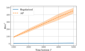
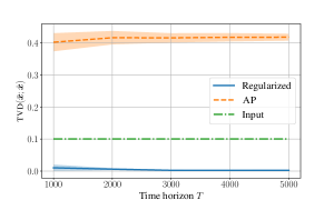
Figure 2: (Left): Empirical upper bound on the regret (i.e., $\textsc{Reg}^{\textsc{u}}$ as defined in Equation 9) for breakdown B2 with prices unbalance. (Right): Total variation distance from the target distribution $\hat{\bm{x}}$ for B2 with prices unbalance.

References

- Agarwal et al. [2014] Deepak Agarwal, Souvik Ghosh, Kai Wei, and Siyu You. Budget pacing for targeted online advertisements at linkedin. In Proceedings of the 20th ACM SIGKDD international conference on Knowledge discovery and data mining, pages 1613–1619, 2014.
- Agrawal and Devanur [2014] Shipra Agrawal and Nikhil R Devanur. Fast algorithms for online stochastic convex programming. In Proceedings of the twenty-sixth annual ACM-SIAM symposium on Discrete algorithms, pages 1405–1424. SIAM, 2014.
- Agrawal et al. [2014] Shipra Agrawal, Zizhuo Wang, and Yinyu Ye. A dynamic near-optimal algorithm for online linear programming. Operations Research, 62(4):876–890, 2014.
- Agrawal et al. [2016] Shipra Agrawal, Nikhil R Devanur, and Lihong Li. An efficient algorithm for contextual bandits with knapsacks, and an extension to concave objectives. In Conference on Learning Theory, pages 4–18. PMLR, 2016.
- Amin et al. [2012] Kareem Amin, Michael Kearns, Peter Key, and Anton Schwaighofer. Budget optimization for sponsored search: Censored learning in mdps. arXiv preprint arXiv:1210.4847, 2012.
- Arlotto and Gurvich [2019] Alessandro Arlotto and Itai Gurvich. Uniformly bounded regret in the multisecretary problem. Stochastic Systems, 9(3):231–260, 2019.
- Avadhanula et al. [2021] Vashist Avadhanula, Riccardo Colini-Baldeschi, Stefano Leonardi, Karthik Abinav Sankararaman, and Okke Schrijvers. Stochastic bandits for multi-platform budget optimization in online advertising. arXiv preprint arXiv:2103.10246, 2021.
- Badanidiyuru et al. [2014] Ashwinkumar Badanidiyuru, John Langford, and Aleksandrs Slivkins. Resourceful contextual bandits. In Conference on Learning Theory, pages 1109–1134. PMLR, 2014.
- Balseiro et al. [2017] Santiago Balseiro, Anthony Kim, Mohammad Mahdian, and Vahab Mirrokni. Budget management strategies in repeated auctions. In Proceedings of the 26th International Conference on World Wide Web, pages 15–23, 2017.
- Balseiro et al. [2020a] Santiago Balseiro, Haihao Lu, and Vahab Mirrokni. The best of many worlds: Dual mirror descent for online allocation problems. arXiv preprint arXiv:2011.10124, 2020a.
- Balseiro et al. [2020b] Santiago Balseiro, Haihao Lu, and Vahab Mirrokni. Dual mirror descent for online allocation problems. In International Conference on Machine Learning, pages 613–628. PMLR, 2020b.
- Balseiro et al. [2020c] Santiago Balseiro, Haihao Lu, and Vahab Mirrokni. Regularized online allocation problems: Fairness and beyond. arXiv preprint arXiv:2007.00514, 2020c.
- Balseiro and Gur [2019] Santiago R Balseiro and Yonatan Gur. Learning in repeated auctions with budgets: Regret minimization and equilibrium. Management Science, 65(9):3952–3968, 2019.
- Balseiro et al. [2015] Santiago R Balseiro, Omar Besbes, and Gabriel Y Weintraub. Repeated auctions with budgets in ad exchanges: Approximations and design. Management Science, 61(4):864–884, 2015.
- Borgs et al. [2007] Christian Borgs, Jennifer Chayes, Nicole Immorlica, Kamal Jain, Omid Etesami, and Mohammad Mahdian. Dynamics of bid optimization in online advertisement auctions. In Proceedings of the 16th international conference on World Wide Web, pages 531–540, 2007.
- Borwein and Lewis [2010] Jonathan Borwein and Adrian S Lewis. Convex analysis and nonlinear optimization: theory and examples. Springer Science & Business Media, 2010.
- Conitzer et al. [2019] Vincent Conitzer, Christian Kroer, Debmalya Panigrahi, Okke Schrijvers, Eric Sodomka, Nicolas E Stier-Moses, and Chris Wilkens. Pacing equilibrium in first-price auction markets. In Proceedings of the 2019 ACM Conference on Economics and Computation, pages 587–587, 2019.
- Conitzer et al. [2021] Vincent Conitzer, Christian Kroer, Eric Sodomka, and Nicolas E. Stier-Moses. Multiplicative pacing equilibria in auction markets. Operations Research (to appear), 2021. URL https://arxiv.org/abs/1706.07151.
- Devanur and Hayes [2009] Nikhil R Devanur and Thomas P Hayes. The adwords problem: online keyword matching with budgeted bidders under random permutations. In Proceedings of the 10th ACM conference on Electronic commerce, pages 71–78, 2009.
- Devanur et al. [2012] Nikhil R Devanur, Balasubramanian Sivan, and Yossi Azar. Asymptotically optimal algorithm for stochastic adwords. In Proceedings of the 13th ACM Conference on Electronic Commerce, pages 388–404, 2012.
- Devanur et al. [2019] Nikhil R Devanur, Kamal Jain, Balasubramanian Sivan, and Christopher A Wilkens. Near optimal online algorithms and fast approximation algorithms for resource allocation problems. Journal of the ACM (JACM), 66(1):1–41, 2019.
- Edelman et al. [2007] Benjamin Edelman, Michael Ostrovsky, and Michael Schwarz. Internet advertising and the generalized second-price auction: Selling billions of dollars worth of keywords. American economic review, 97(1):242–259, 2007.
- eMarketer [2020] eMarketer. eMarketer us digital ad spending update q2 2020. https://www.emarketer.com/content/us-digital-ad-spending-update-q2-2020, 2020. Accessed: 2020-02-03.
- Feldman et al. [2007] Jon Feldman, Shanmugavelayutham Muthukrishnan, Martin Pal, and Cliff Stein. Budget optimization in search-based advertising auctions. In Proceedings of the 8th ACM conference on Electronic commerce, pages 40–49, 2007.
- Feldman et al. [2009a] Jon Feldman, Nitish Korula, Vahab Mirrokni, Shanmugavelayutham Muthukrishnan, and Martin Pál. Online ad assignment with free disposal. In International workshop on internet and network economics, pages 374–385. Springer, 2009a.
- Feldman et al. [2009b] Jon Feldman, Aranyak Mehta, Vahab Mirrokni, and Shan Muthukrishnan. Online stochastic matching: Beating 1-1/e. In 2009 50th Annual IEEE Symposium on Foundations of Computer Science, pages 117–126. IEEE, 2009b.
- FICO [2021] FICO. Xpress optimization suite, 2021. URL https://www.fico.com/en/products/fico-xpress-optimization.
- Gelauff et al. [2020] Lodewijk Gelauff, Ashish Goel, Kamesh Munagala, and Sravya Yandamuri. Advertising for demographically fair outcomes. arXiv preprint arXiv:2006.03983, 2020.
- Goel and Mehta [2008] Gagan Goel and Aranyak Mehta. Online budgeted matching in random input models with applications to adwords. In SODA, volume 8, pages 982–991, 2008.
- Gummadi et al. [2013] Ramki Gummadi, Peter Key, and Alexandre Proutiere. Optimal bidding strategies and equilibria in dynamic auctions with budget constraints. Available at SSRN 2066175, 2013.
- Hosanagar and Cherepanov [2008] Kartik Hosanagar and Vadim Cherepanov. Optimal bidding in stochastic budget constrained slot auctions. In Proceedings of the 9th ACM Conference on Electronic Commerce, pages 20–20, 2008.
- Jasin [2015] Stefanus Jasin. Performance of an lp-based control for revenue management with unknown demand parameters. Operations Research, 63(4):909–915, 2015.
- Li and Ye [2019] Xiaocheng Li and Yinyu Ye. Online linear programming: Dual convergence, new algorithms, and regret bounds. arXiv preprint arXiv:1909.05499, 2019.
- Li et al. [2020] Xiaocheng Li, Chunlin Sun, and Yinyu Ye. Simple and fast algorithm for binary integer and online linear programming. arXiv preprint arXiv:2003.02513, 2020.
- Mahdian et al. [2012] Mohammad Mahdian, Hamid Nazerzadeh, and Amin Saberi. Online optimization with uncertain information. ACM Transactions on Algorithms (TALG), 8(1):1–29, 2012.
- Mehta et al. [2007] Aranyak Mehta, Amin Saberi, Umesh Vazirani, and Vijay Vazirani. Adwords and generalized online matching. Journal of the ACM (JACM), 54(5):22–es, 2007.
- Mirrokni et al. [2012] Vahab S Mirrokni, Shayan Oveis Gharan, and Morteza Zadimoghaddam. Simultaneous approximations for adversarial and stochastic online budgeted allocation. In Proceedings of the twenty-third annual ACM-SIAM symposium on Discrete Algorithms, pages 1690–1701. SIAM, 2012.
- Nasr and Tschantz [2020] Milad Nasr and Michael Carl Tschantz. Bidding strategies with gender nondiscrimination constraints for online ad auctions. In Proceedings of the 2020 Conference on Fairness, Accountability, and Transparency, pages 337–347, 2020.
- Orabona [2019] Francesco Orabona. A modern introduction to online learning. arXiv preprint arXiv:1912.13213, 2019.
- Varian [2007] Hal R Varian. Position auctions. International Journal of industrial Organization, 25(6):1163–1178, 2007.
- Wu et al. [2018] Di Wu, Xiujun Chen, Xun Yang, Hao Wang, Qing Tan, Xiaoxun Zhang, Jian Xu, and Kun Gai. Budget constrained bidding by model-free reinforcement learning in display advertising. In Proceedings of the 27th ACM International Conference on Information and Knowledge Management, pages 1443–1451, 2018.
- Xu et al. [2015] Jian Xu, Kuang-chih Lee, Wentong Li, Hang Qi, and Quan Lu. Smart pacing for effective online ad campaign optimization. In Proceedings of the 21th ACM SIGKDD International Conference on Knowledge Discovery and Data Mining, pages 2217–2226, 2015.
- Zhang et al. [2012] Weinan Zhang, Ying Zhang, Bin Gao, Yong Yu, Xiaojie Yuan, and Tie-Yan Liu. Joint optimization of bid and budget allocation in sponsored search. In Proceedings of the 18th ACM SIGKDD international conference on knowledge discovery and data mining, pages 1177–1185, 2012.
- Zhang et al. [2014] Weinan Zhang, Shuai Yuan, and Jun Wang. Optimal real-time bidding for display advertising. In Proceedings of the 20th ACM SIGKDD international conference on Knowledge discovery and data mining, pages 1077–1086, 2014.
- Zhang et al. [2016] Weinan Zhang, Yifei Rong, Jun Wang, Tianchi Zhu, and Xiaofan Wang. Feedback control of real-time display advertising. In Proceedings of the Ninth ACM International Conference on Web Search and Data Mining, pages 407–416, 2016.
- Zhou et al. [2008] Yunhong Zhou, Deeparnab Chakrabarty, and Rajan Lukose. Budget constrained bidding in keyword auctions and online knapsack problems. In International Workshop on Internet and Network Economics, pages 566–576. Springer, 2008.