Maximum Entropy Spectral Analysis: a case study

The Maximum Entropy Spectral Analysis (MESA) method, developed by Burg, provides a powerful tool to perform spectral estimation of a time-series. The method relies on a Jaynes’ maximum entropy principle and provides the means of inferring the spectrum of a stochastic process in terms of the coefficients of some autoregressive process AR($p$) of order $p$. A closed form recursive solution provides an estimate of the autoregressive coefficients as well as of the order $p$ of the process. We provide a ready-to-use implementation of the algorithm in the form of a python package memspectrum. We characterize our implementation by performing a power spectral density analysis on synthetic data (with known power spectral density) and we compare different criteria for stopping the recursion. Furthermore, we compare the performance of our code with the ubiquitous Welch algorithm, using synthetic data generated from the released spectrum by the LIGO-Virgo collaboration. We find that, when compared to Welch’s method, Burg’s method provides a power spectral density (PSD) estimation with a systematically lower variance and bias. This is particularly manifest in the case of a little number of data points, making Burg’s method most suitable to work in this regime.

1 Introduction

The study of the properties of stochastic processes is a crucial task in many fields of physics, astronomy, quantitative biology, as well as engineering and finance. Among those, a special place is occupied by the so-called wide-sense stationary processes. These are stochastic processes that display an invariance of their statistical properties, such as their two-point autocovariance function, with respect to time translation. If $x(t)$ is a wide-sense stationary process, it is completely determined by the knowledge of the autocorrelation function

$$C(\tau)=\mathbf{E}[x_{t}\cdot x_{t+\tau}]$$ (1)

or, equivalently, by the knowledge of their power spectral density (PSD) $S(f)$. Thanks to the Wiener-Khinchin theorem the two are related by a Fourier transform:

$$S(f)=\int_{-\infty}^{\infty}\textrm{d}\tau C(\tau)e^{-i2\pi f\tau}\,.$$ (2)

In some literature, especially in the context of gravitational waves physics, e.g.  (Finn 1992), the PSD is introduced as

$$\mathbf{E}[\tilde{x}(f)\cdot\tilde{x}(f^{\prime})]=S(f)\delta(f-f^{\prime})$$ (3)

without highlighting its connection with the time structure of the process itself, thus masking some important properties that will be explored further in what follows. The latter definition in (3) gives, however, i) a straightforward interpretation of the PSD: it measures how much signal “power” is located in each frequency; ii) an operative way of estimating it for an unknown process.

An ubiquitous method for such computation is due to Welch (1967) and it is based on Eqs.(2-3). The PSD is obtained by slicing the observed realization $x(t_{1}),\ldots,x(t_{n})$ of the process $x(t)$ into many window-corrected batches and averaging the squared moduli of their Fourier transforms. This approach is equivalent (Lomb 1976; Scargle 1982) to taking the Fourier Transform of the windowed sample autocorrelation $\rho_{W}$, written as

$$\rho_{W}=\left\{W_{0}\rho_{0},W_{\pm 1}\rho_{\pm 1},\dots,W_{\pm M}\rho_{\pm M},0,0,\dots\right\},$$ (4)

where $\rho$ is the empirical autocorrelation and $M$ is the maximum time lag at which the autocorrelation is computed. The sequence $W$ is a window function that can be chosen in several different ways, each choice presenting advantages and disadvantages for the final estimate of the PSD.

The choice of a window function is arbitrary and typically is made by trial and error, until a satisfactory compromise between variance and resolution of the estimate of PSD is reached. A high frequency resolution implies high variance and vice-versa. Besides the window function, Welch’s method requires a number of arbitrary choices to be made, such as the number of time slices and the overlap between consecutive slices. All these knobs must be tuned by hand and their choice can dramatically affect the PSD estimation, hence begging the question of what the “best” PSD estimate is.

Another drawback of this approach is the requirement for the window to be $0$ outside the interval in which the autocorrelation is computed. We are arbitrarily assuming $\rho_{j}=0$ for $j>M$ and modifying the estimate (i.e. the data) if a non-rectangular window is chosen. Making assumptions on unobserved data and modifying the ones we have at our disposal introduces “spurious” information about the process that we, in general, do not really have.

A alternative approach providing a smooth PSD estimation, is to adopt a parametric model for the PSD and to fit its parameters to the data with a Markov Chain Monte Carlo (Cornish & Littenberg 2015; Littenberg & Cornish 2015, e.g.). Despite being effective, this method is problem dependent, since it needs to make definite assumptions on the shape of the PSD. Moreover, it can be computationally expensive and it does not come with an handy implementation available to the public. For all the above reasons, we did not consider such method in our work.

An appealing alternative, based on the Maximum Entropy principle (Jaynes 1957; Jaynes & Bretthorst 2003; Jaynes 1982), has been put forward by Burg (1975). Being rooted on solid theoretical foundations, we will see that Burg’s method, unlike Welch’s, does not require any preprocessing of the data and requires very little tuning of the algorithm parameters, since it provides an iterative closed form expression for the spectrum of a stochastic stationary time series. Furthermore, it embeds the PSD estimation problem into an elegant theoretical framework and makes minimal assumptions on the nature of the data. Lastly and most importantly, it provides a robust link between spectral density estimation and the field of autoregressive processes. This provides a natural and simple machinery to forecast a time series, thus predicting future observations based on previous ones.

In this paper, we discuss the details of the Maximum entropy principle, its application to the problem of PSD estimation with Burg’s algorithm and the link between Burg’s algorithm and autoregressive process. Our goal is to bring (again) to public attention Maximum Entropy Spectral analysis, in the hope that it will be widely employed as a way out to the many undesired aspects of the Welch’s algorithm (or other similar methods). To facilitate this goal, we present and describe a new code, memspectrum, that provides a robust and easy-to-use python implementation of the algorithm. We provide a thorough assessment of the performance of our code and we validate our results performing a number of tests on simulated and real data. We also compare our results with those of spectral analysis carried out with the standard Welch’s method. In order to apply our model on a realistic setting, we analyse some time series of broad interest in the scientific community.

Our paper is organized as follows: we begin by briefly reviewing the theoretical foundations of the maximum entropy principle in Sec. 2. Sec. 3 presents the validation of Burg’s method as well as of our implementation on simulated data. In Sec. 4 we compare the results from memspectrum with the Welch method; Sec. 5 presents a few applications to real time series and, finally, we conclude with a discussion in Sec. 6.

2 Theoretical foundations

The Maximum Entropy principle (MAXENT) is among the most important results in probability theory. It provides a way to uniquely assign probabilities to a phenomenon in a way that best represent our state of knowledge, while being non committal with unavailable information. Its domain of application turned out to be wider than expected. In fact, thanks to Burg (1975), this method has also been applied to perform high quality computation of power spectral densities of time series.

After a short introduction to Jaynes’ MAXENT (sec. 2.1), we will develop in detail Burg’s technique of Maximum Entropy Spectral Analysis (MESA) and show that the estimate can be expressed in an analytical closed form (sec. 2.2). Next, we will discuss an interesting link between Burg’s method and autoregressive processes (sec. 2.3) and in sec. 2.4 we will use such link for straightforwardly forecasting a time series.

2.1 Maximum Entropy Principle

Before introducing MAXENT principle, we will define through some simple examples the two core concepts of the problem and the role they play: the ‘evidence’ and the ‘information’. Let us start with the ‘information’ (or entropy): it is a measure of the degree of uncertainty on the outcomes of some experiment and specifies the length of the message necessary to provide a full description of the system under study. For instance, consider a perfectly sinusoidal signal: knowledge of amplitude, frequency and phase are sufficient to fully reproduce it: it has a low information content. Even less information is required if we are studying a system whose outcome is certain (has probability $p=1$), as in this case, a communication is not even needed. Shannon (1948) proposed the quantity

$$I=\log_{2}\frac{1}{p(x)}$$ (5)

to measure the quantity of information brought by an outcome $x$ with probability $p(x)$. It is additive quantity as well as monotonically decreasing as a function of $p\in[0,1]$: the more uncertain the outcome, the higher the information it brings.

We can generalize the definition of information in the case where two different outcomes $E_{1},E_{2}$, with given probabilities $P_{1}$ and $P_{2}$, are possible. To gain some intuition on the problem, we ask ourselves which are the probability assignments that make the outcome more uncertain (i.e. maximize the information). If $P_{1}$ and $P_{2}$ are largely different, for instance $P_{1}=0.999$ and $P_{2}=0.001$, we are allowed to believe that event $E_{1}$ will occur almost certainly, considering $E_{2}$ to be a very implausible outcome. The information content will be very low. On the other hand, most unpredictable experiment happens when

$$P_{1}=P_{2}=\frac{1}{2}:$$

this describes a situation of ‘maximum ignorance’ and the information content of such system must be high. Any generalization of eq. (5), must then have its maximum when $P_{1}=P_{2}$. For $N$ events, the system with the highest possible information content is when:

$$P_{1}=\ldots=P_{N}=\frac{1}{N}:$$

Shannon (1948) showed that the only functional form satisfying continuity with respect to its parameters, additivity and that has a maximum for equal probability events is:

$$H[p_{1},\dots,p_{N}]=-\sum_{i=1}^{N}p_{i}\log{p_{i}},$$ (6)

The equation can be interpreted as the ‘expected information’ brought by an experiment with $N$ possible outcomes each with its own probability $p_{i}$. In the continuous case:

$$H[p(x)]=-\int p(x)\ln p(x)dx,$$ (7)

We call the functional $H$ (information) entropy.

We now turn to the core of our problem: how do we make a probability assignment for a set of events, that keeps into account our knowledge of the system and, at the same time, it is non committal towards unavailable knowledge? The knowledge at our disposal about the system under study is what we call ‘evidence’ and any probability assignment must agree with it. In the above cases, our knowledge on the system is only the total number $N$ of different outcomes – this is a minimal requirement. Of course, more complex evidence constraints can be applied.

It is very common that the constraints provided by the evidence are not enough for setting the probabilities for each event: in this case, it is reasonable to assume that the probability assignment should make the experiment as unpredictable as possible. In other words, the amount of ‘information’ introduced by the probability assignment should be as high as possible.

MAXENT puts the aforementioned principle into a more precise mathematical context by stating that probabilities should be assigned by maximizing uncertainty (information entropy) using evidence as constraint. This defines a variational problem, where the information entropy functional $H\left[p_{1},\dots,p_{N}\right]$, defined in eq. (6), has to be maximized.

The maximisation of entropy, supplemented by evidence in the form of constraints to which the sought-for probability distribution must obey, gives rise to several of the most common probability distributions commonly employed in statistics. For instance, whenever the only constraint available is the normalization of the probability distribution (i.e. no evidence is available), the entropy is maximised by the uniform distribution. If we have evidence to constraint the expected value, the information entropy is maximised by the exponential distribution

Of particular importance is the case in which, in addition to the mean, also the variance is known: MAXENT leads to the Gaussian distribution. This derivation is particularly interesting from the foundational point of view, since it provides a deeper insight into the ubiquitous Gaussian distribution. Indeed, it is not only the limit distribution provided by the central limit theorem for finite variance processes but it is also the distribution that maximizes the entropy. For this reason, appealing to MAXENT principle, it is the correct assignment if mean and covariance are the only quantities that fully define our process. In some sense, we can interpret the central limit theorem as the natural ‘statistical’ evolution toward a configuration that maximizes entropy.

For this work, we are particularly interested in the multi-dimensional case. Suppose we have a vector of measurements $(x(t_{1}),\ldots,x(t_{n}))=(x_{1},\ldots,x_{n})$ that we conveniently express as a single realization of an unknown stochastic process $x(t)$ and we have information about the expectation value of the process $\mu(t)$ and on the matrix of autocovariances $C_{ij}\equiv C(t_{i},t_{j})$, then the MAXENT distribution is the $n$-dimensional multivariate Gaussian distribution (Gregory 2005):

$$p \left((x_{1},\ldots,x_{n})|I\right)=$$

$$\frac{1}{\left(2\pi\det C\right)^{k/2}}\exp\left(-\frac{1}{2}\sum_{i,j}(x_{i}-\mu_{i})(x_{j}-\mu_{j})C^{-1}_{ij}\right)\,.$$ (8)

For a wide-sense stationary process the mean function is independent of time, hence it can be redefined to be equal to zero without loss of generality, and the auto-covariance function is dependent only on the time lag $\tau\equiv t_{i}-t_{j}$. One can thus choose a sampling rate $\Delta t$ so that $C_{ij}=C((i-j)\Delta t)$. The autocovariance matrix thus becomes a Toeplitz matrix. Toeplitz matrices are asymptotically equivalent to circulant matrices and thus diagonalized by the discrete Fourier transform base (Gray 2006). Some simple algebra shows that the time-domain multivariate Gaussian can be transformed into the equivalent frequency domain probability distribution:

$$p \left((\tilde{x}_{1},\ldots,\tilde{x}_{n/2})|I\right)=$$

$$\frac{1}{\left(2\pi\det S\right)^{n/2}}\exp\left(-\frac{1}{2}\sum_{ij}\tilde{x}_{i}S^{-1}_{ij}\tilde{x}_{j}\right)\,,$$ (9)

where the matrix $S_{ij}=S_{i}\delta_{ij}$ is an $n\times n$ diagonal matrix whose elements are the PSD $S(f)$ calculated at frequency $f_{i}$. Many readers will recognize the familiar form of the Whittle likelihood that stands at the basis of the matched filter method(P. M. Woodward & Higinbotham 1964) and of gravitational waves data analysis, (Finn 1992; Allen et al. 2012, e.g.). Thanks to MAXENT, the problem of defining the probability distribution describing a wide-sense stationary process is thus entirely reduced to the estimation of the PSD or, equivalently, the autocovariance function.

2.2 Maximum Entropy Spectral Analysis

In principle, if the autocorrelation was known exactly (i.e. at every time $\tau\in(-\infty,+\infty)$), the computation of the PSD would reduce to a single Fourier transform. However, in any realistic setting, we are dealing with a finite number of samples $N$ from the process, hence such computation is impossible. Moreover, the error $\sigma_{k}$ in the estimate of the autocorrelation after $k$ steps increases as $\sigma\sim 1/\sqrt{N-k}$, so that only few values for the autocorrelation function can actually be computed reliably. This bring us the core of the problem: how to give an estimate from partial (and noisy) knowledge of the autocorrelation function? MAXENT can guide us in this task without any a priori assumptions on the unavailable data.

As in the previous examples, one needs to set up a variational problem where the entropy, Eq. (7), is maximized subject to some problem-specific constraints. In our case, they are i) the PSD estimate has to be non-negative; ii) its Fourier transform has to match the sample autocorrelation (wherever an estimate of this is available).

Before doing so, there is a technicality to solve: the definition of entropy depends on a probability distribution, not on the PSD. It can be shown,  (Ables 1974; Bartlett 1968, e.g.), that the variational problem can be formulated in terms of the power spectral density $S(f)$ alone by considering our signal as the result of the filtering a white noise process using a filter with transfer function $T(f)$ equal to $S(f)$. The difference in entropy between the input and the output time series (i.e. the entropy gain) obtained by such filter applied on white noise is:

$$\Delta H=\int_{-Ny}^{Ny}\log S(f)df\,.$$ (10)

where $\Delta t$ is sampling rate and $Ny\equiv\frac{1}{2\Delta t}$ is the Nyquist frequency. Thus maximising Eq. (10) is equivalent to maximizing eq. (7).

Before maximizing the entropy gain, we need to include the evidence available as a form of mathematical constraints for the assignment of $S(f)$. This is equivalent in imposing that the variational solution $S(f)$ for the PSD matches the empirical autocorrelation. Let us define a realization of a stochastic process $(x_{1},\ldots,x_{N})$ with sample autocorrelations $\bar{r}_{k},\,k=0,\ldots,N/2$, then the PSD must satisfy the following equation:

$$\int_{-Ny}^{Ny}S(f)e^{\imath 2\pi fk\Delta t}df=\bar{r}_{k}\,.$$ (11)

Thus, by maximizing Eq. (10) with constraints in Eq. (11), we can give an estimate of the spectrum given an empirical time series. This approach on PSD computation provides a result consistent with the empirical autocorrelation function whenever this is available and, at the same time, it does not make any assumption for the unavailable estimates for the autocorelation at large time lags.

Most importantly, the variational problem admits a closed-form analytical expression for $S(f)$. The expression was first found by  Burg (1975):

$$S(f)=\frac{P_{N}\Delta t}{\left(\sum_{s=0}^{N}a_{s}z^{s}\right)\left(\sum_{s=0}^{N}a^{*}_{s}z^{-s}\right)},$$ (12)

where $\Delta t$ is the sampling interval of the time series, $z=\exp{(2\pi if\Delta t)}$, $a_{0}$ = 1. The vector obtained as $(1,a_{1},\dots,a_{N})$ is also known as the prediction error filter. The coefficients $a_{s}(s>0)$, together with an overall multiplicative scale factor $P_{N}$, are to be determined by an iterative process (called Burg’s algorithm). The number $N$ of such coefficients is a choice that shall be made by the user and indeed it is the only hyperparameter that needs to be tuned. The details of the derivation and the actual form for the coefficients $a_{s}$ can be found in appendix A.

2.3 Autoregressive Process Analogy

The application of MESA is not limited to spectral estimates, but it also provides a link between spectral analysis and the study of autoregressive processes (AR) (Ulrych & Bishop 1975). An autoregressive stationary process of order $p$, AR($p$), is a time series whose values satisfy the following expression:

$$x_{t}-b_{1}x_{t-1}-b_{2}x_{t-2}\dots b_{p}x_{t-p}=\nu_{t}$$ (13)

where $b_{1},\ldots,b_{p}$ are real coefficients and $\nu_{t}$ is white noise with a given variance $\sigma^{2}$. Thus, an AR($p$) process models the dependence of the value of the process at time $t$ on every past $p$ observations, thus being potentially able to model complex autocorrelation structures within observations.

Thanks to Wold’s theorem (Wold 1939), every stationary time series can be represented as an autoregressive process: this ensures that maximum entropy estimation is faithful and general; it turns out that the maximum entropy principle provides a representation of the time series as an $AR(p)$ process and Burg’s algorithm computes the autoregressive coefficients that are suitable to the available data.

To show the analogy, we compute the PSD $S_{AR(p)}$ of an $AR(p)$ process and we show that it is formally equivalent to the PSD obtained in Eq. (12). This will also provide a direct expression for the autoregressive coefficients $b_{i}$ and for the noise variance $\sigma^{2}$. We start taking the $z$ transform  of Eq. (13):

$$\sum_{t}x_{t}z^{t}-\sum_{i}b_{i}z^{i}\sum_{t}x_{t-i}z^{t-i}=\sum_{t}\nu_{t}z^{t}.$$ (14)

Calling $\tilde{x}(z)$ and $\tilde{\nu}(z)$, the transformed quantities, in the $z$ domain, the process takes the form:

$$\tilde{x}(z)=\frac{\tilde{\nu}(z)}{\left(1-\sum_{n=1}^{p}b_{n}z^{n}\right)}$$ (15)

Since we assumed a wide-sense stationary process, $\tilde{x}(z)$ is analytic both on and inside the unit circle. Taking its square value and evaluating it on the unit circle $z=e^{-\imath 2\pi f\Delta t}$, from the definition of spectral density one obtains:

$$S_{AR(p)}(f)=|\tilde{x}(z)|^{2}=\frac{|\tilde{\nu}(f)|^{2}}{\left|1-\sum_{n=1}^{p}b_{n}e^{\imath 2\pi fn\Delta t}\right|^{2}}\,.$$ (16)

The numerator is the spectral density of white noise $\nu_{t}$, i.e. its (constant) variance $\sigma^{2}$.

Eqs. (16) and  (12) are equivalent, if we identify $b_{i}=-a_{i}$ and $P_{N}\Delta t=\sigma^{2}$. This shows that the MAXENT estimation of the PSD models the observed times series as an AR process and provides a fit for the autoregressive coefficients. Furthermore, as a consequence of Wold’s theorem, there is the theoretical guarantee that every stationary time series can be modelled faithfully by the MAXENT.

2.4 Forecasting

The link between MESA and AR processes is of particular interest. Given the solution to Burg’s recursion to determine the $a_{k}$, we automatically obtain the coefficients of the equivalent AR process, hence we are able to exploit Eq. 13 to perform forecasting, thus providing plausible future observations, conditioned on the observed data. Indeed, for an AR($p$) process the conditional probability $p(x_{t}|x_{t-1},\ldots,x_{t-p})$ of the observation at time $t$ with respect to the past $p$ observation has the form:

$$p (x_{t}|x_{t-1},\ldots,x_{t-p})$$

$$=\frac{1}{\sigma\sqrt{2\pi}}\exp\left[-\frac{1}{2}\left(\frac{x_{t}-\sum_{i=1}^{p}b_{i}x_{t-i}}{\sigma}\right)^{2}\right]\,.$$ (17)

The interpretation of Eq. (2.4) is straightforward: $x_{t}$ follows a Gaussian distribution with a fixed variance and a mean value $m_{t}=\sum_{i=1}^{p}b_{i}x_{t-i}$ computed from past observations. Eq. (2.4) provides then a well defined probability framework for predicting future observations: this is a very useful feature of MESA, that does not have an equivalent in any other spectral analysis computation methods.

3 Validation of the model

It is now clear that MESA provides a recursive formula for computing the coefficients $a_{k}$ in Eq. (12). The number $M$ of such coefficients is equivalent to the maximum order of the autocorrelation $\bar{r}_{m}$ considered. In an ideal scenario, this would be equal to the number of points the autocorrelation is computed at (equivalent to the length of data considered). However, the computation of high order coefficients of the autocorrelation is unstable and for high enough $m$, as the estimation for $\bar{r}_{m}$ shows a very high variance, broadly scaling as $\sim\left(\sqrt{M-m}\right)^{-1}$.

It is then clear that the choice of the number of samples of the discrete autocorrelation to consider is important: on the one hand it is advisable to include as much knowledge of the autocorrelation as possible, leading to include all the known $\bar{r}_{m}$; on the other hand, including values of the autocorrelation that are not reliably estimated, can be counterproductive. The order $M$ of the autocorrelation to be considered (or, equivalently, the order $M$ of the underlying autoregressive process) is the only tuning parameter of MESA and a careful balance between these two necessities must be made when applying the algorithm.

The remainder of this section is devoted to an extensive study on how to make such choice. In Section 3.1, we are going to define three different loss functions to measure how well the algorithm is able to reproduce a known PSD. The basic idea is to validate, as the autoregressive order considered increases, the performance of the algorithm results by measuring the loss function and pick, among the orders the one that yields better results. Second, the performance of different loss functions will be assessed by performing the spectral analysis on time series with an analytical Gaussian PSD, sec. 3.2. In a last subsection 3.3, the same analysis is performed on synthetic data generated from the analytical spectrum released by the LIGO-Virgo collaboration.

3.1 Choice of the autoregressive order

Guided from numerical experiments, an indication on the upper bound to the autoregressive order $M_{max}$ is (Berryman 1978):

$$M_{max}=2N/\ln{(2N)}\,,$$ (18)

where $N$ is the number of observed points in the time-series. However, this is just a plausible upper limit on the order of the AR process $m$ and the optimal algorithm could employ fewer points. We then need a more sophisticated method for computing the right value for $m$. Various loss functions to assess the algorithm performance have been proposed in literature. We summarise them below:

• Final prediction Error The first criterion is due to  Akaike (1998). It was proposed that $m$ should be chosen as the length that minimizes the error when the filter is used as a predictor, the final prediction error (FPE):

  $$FPE(m)=\mathbb{E}\left[\left((x_{t}-\hat{x}_{t})^{2}\right)\right]$$ (19)

  with $\hat{x}_{t}=\sum_{i=1}^{M}a_{i}x_{t-i}$. Minimizing FPE is equivalent to minimizing the quantity:

  $$\mathcal{L}_{\rm FPE}(m)=P_{m}\frac{N+m+1}{N-m-1}$$ (20)

  with $P_{m}$ being the estimated noise variance at order $m$, see Eq. (35). In the $N\to\infty$ limit, remembering $m_{max}\sim 2N/\log(2N)$, Akaike’s loss function is equivalent to the minimization of the variance $P_{m}$ of the white noise of the underlying $AR(p)$ model.

• Criterion Autoregressive Transfer function (CAT) This second loss function has been proposed by Parzen and studied in detail by Bhansali (1986). It is based on the assumption that the observed process is an infinite order autoregressive process

  $$x_{t}=\sum_{i=1}^{\infty}a_{i}x_{t-i}+\nu_{t}$$ (21)

  and tries to select the order $m$ as the best finite-order approximation for the observed process. Being N the number of samples it has the property that $m\to\infty$ as $N\to\infty$. Since any real-valued stochastic process can be written as a ARMA(p,q) process (Wold theorem) i.e. an $AR(\infty)$ process, this is a physically significant property. The loss function has the functional form:

  $$\mathcal{L}_{\rm CAT}(m)=\frac{1}{N}\sum_{k=1}^{m}\frac{N-k}{NP_{k}}-\frac{N-m}{NP_{m}},$$ (22)

  and the so-chosen order is found to be asymptotically unbiased for $P_{N}$.

• Optimum Bayes Decision rule The last criterion we will consider is the Optimum Bayes Decision rule (OBD)(Rao et al. 1982). Let $x(t)$ be the observed time series for the process that has to be described as an $AR(m)$ process, with $m$ to be determined. The OBD is obtained choosing between M different hypothesis $H_{i},i=1,\dots,M$ maximizing their posterior distribution $P(H_{i}|x(t))$. Each hypothesis is uniquely determined from both the length and the values of the filter under study. Choosing a Likelihood of the form Eq. (2.4) and uniform priors for both the coefficients and the hypotheses, Rao has shown that choosing the minimum for $-log(P(H_{i}|x(t))$, i.e. maximizing the posterior for $H_{i}$, is asymptotically equivalent to the minimization of:

  $$\mathcal{L}_{\rm OBD} (m)=(N-m-2)\log(P_{m})$$

  $$+m\log(N)+\sum_{k=0}^{m-1}\log(P_{k})+\sum_{k=1}^{m}a_{k}^{2}\,.$$ (23)

Once a loss function is selected, the choice of the best recursion order is straightforward: we solve the Levinson recursion (Levinson 1946) until $M_{max}$, as given in Eq. (18), iterations are reached. Then, the order $m$ is selected to be the one that minimizes the specified loss function.

In a real implementation of the algorithm, computing all the recursion up to $M_{max}$ can result in a significant waste of computational power: the optimal value is often $m_{opt}<<M_{max}$ and, in such cases, computing all the values of $m$ until $M_{max}$ is not useful. In practice, we can apply an early stop procedure: every few iterations we look for the best order of $m_{opt}$; if this value does not change for a while, we assume that a good (local) minimum of the loss function is found and the computation is stopped.

The following sections will be devoted to the study of the statistical properties of the loss functions introduced above: we need to understand which choice provides the best quality in the reproduction of some known power spectral densities.

3.2 Choice of the loss function: Gaussian PSD

We test the performance of the three loss functions on a random time series generated with a known power spectral density. In this first experiment, we take the PSD to be a Gaussian distribution with mean $\mu=2.5$ and standard deviation $\sigma=0.5$, where the units are arbitrary. The time series are generated by sampling a frequency vector from ${p(\tilde{n}(f_{i}))\propto\exp{\left\{-\frac{1}{2}\sum_{i}\frac{n_{i}^{2}}{S(f_{i})}\right\}}}$ and performing an inverse Fast Fourier Transform on the frequency series. For this investigation, we generate a dataset of $N=1000$ time series of $3000$ points each.

We then apply Burg’s method choosing in turn each of the loss functions on the ensemble of simulated time series, thus obtaining an ensemble of PSD estimates. Through these ensembles, we characterize statistically the performance of each loss function. The disagreement between the PSD $S_{i}(f)$ estimated from the $i$-th simulated time series and the target PSD $S(f)$ is measured via the frequency-averaged relative error $r_{i}$:

$$r_{i}=\frac{1}{N_{f}}\sum_{f_{j}=\{0,\ldots,Ny\}}\frac{|S_{i}(f_{j})-S(f_{j})|}{S(f_{j})}$$ (24)

where $Ny$ is the Nyquist frequency of the time series and $N_{f}$ is the number of the discrete frequencies the PSD is evaluated at.

For each loss function, we compute the ensemble-averaged PSD (as well as the $90\%$ confidence level) and the ensemble-averaged relative error:

$$r(f)=\frac{1}{N}\sum_{i}\frac{|S_{i}(f)-S(f)|}{S(f)}\;.$$ (25)

For each loss function, Figs. 1 2 and 3 show the averaged PSD, as well as the ensemble-averaged relative error from Eq. (25). Furthermore, Fig. 4 displays the relation between $r_{i}$ and the autoregressive order $m_{i}$ chosen for each independently drawn time series.

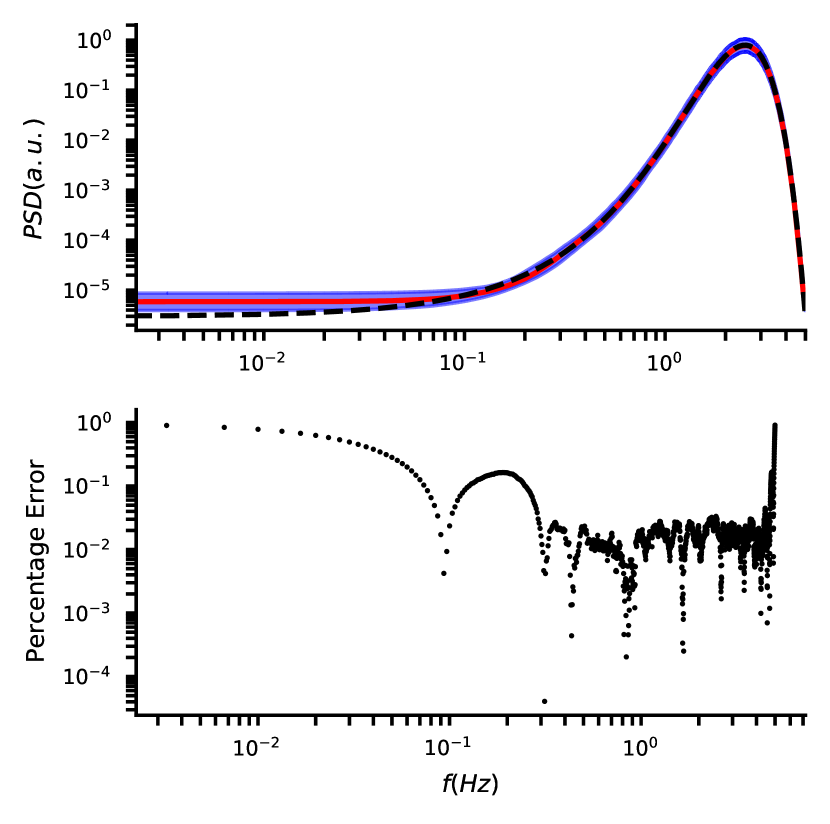
Figure 1: In the top panel, we show the average spectrum for $\mathcal{L}_{\rm FPE}(m)$ with 90% confidence regions (purple shaded region), together with the median estimation (red line) and the target PSD (black dashed line). In the bottom panel, we display the ensemble-averaged relative error eq. (25). The average is computed with $1000$ realization of a $3000$ points long time series.

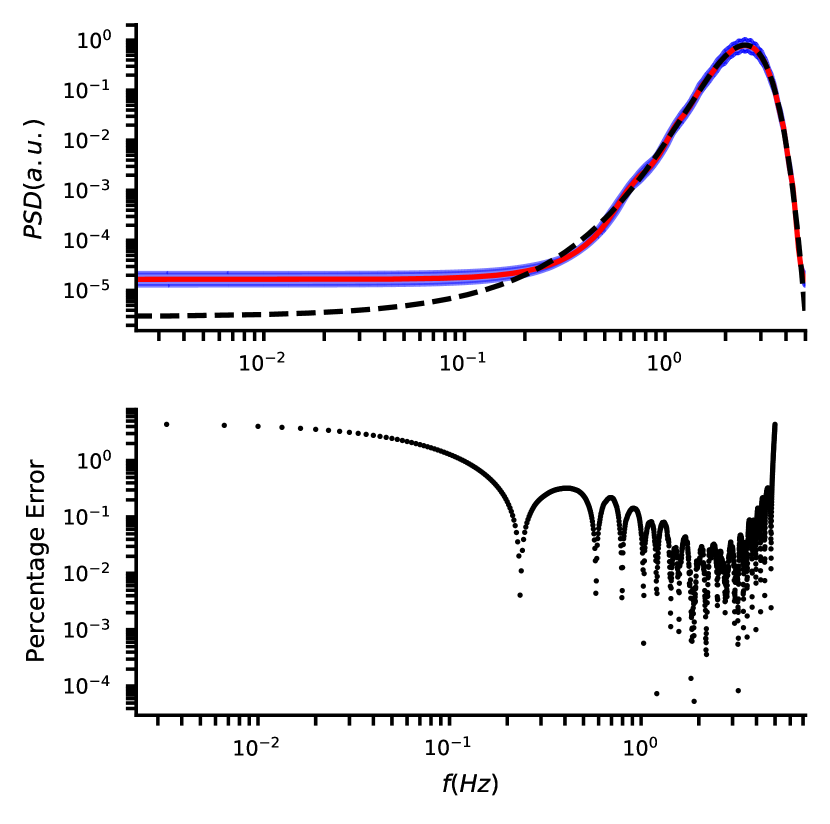
Figure 2: In the top panel, we show the average spectrum for $\mathcal{L}_{\rm OBD}(m)$ with 90% confidence regions (purple shaded region), together with the median estimation (red line) and the target PSD (black dashed line). In the bottom panel, we display the ensemble-averaged relative error eq. (25). The average is computed with $1000$ realization of a $3000$ points long time series.

Figure 3: In the top panel, we show the average spectrum for $\mathcal{L}_{\rm CAT}(m)$ with 90% confidence regions (purple shaded region), together with the median estimation (red line) and the target PSD (black dashed line). In the bottom panel, we display the ensemble-averaged relative error eq. (25). The average is computed with $1000$ realization of a $3000$ points long time series.

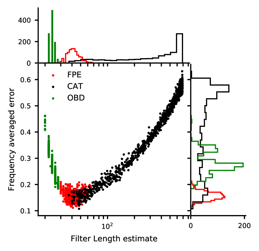
Figure 4: Frequency-averaged relative error $r$ eq. (24) vs the length $m$ of autoregressive process, for each of the $1000$ independent realizations of the synthetic time series with a gaussian PSD. Different colours refers to different choices for the loss function: in red $\mathcal{L}_{\rm FPE}(m)$, in green $\mathcal{L}_{\rm OBD}(m)$ and in black $\mathcal{L}_{\rm CAT}(m)$. The top and right histograms show the marginal distributions.

Final Prediction Error (FPE)

The results of our investigation on the performance of FPE are shown in Fig. 1. Qualitatively, there is a good agreement between the reconstructed spectrum and the true spectrum; however, we note that the reconstruction is not very accurate in the low frequency region. Furthermore, the $90\%$ credible region is very small: this means that if we randomly take two of the reconstructed spectra, we expect their differences to be statistically small. These facts are evidence for FPE to be a reliable loss function.

By looking at Fig. 4 (red series), we note that the AR orders obtained with FPE are clustered in a very small region. This is also a desirable property: FPE, in fact, provides a stable estimation of the AR order, which does not affect much the reconstruction error. We conclude that the FPE shows good quality reconstruction for the spectrum and very desirable stability properties, its estimate for filter’s length $m$ is clustered in a region where there is no dependence of error on $m$.

Optimum Bayes Decision Rule (OBD)

The second loss function we consider is OBD and the results are summarized in Fig. 2. As for the FPE case, they show a good agreement between the average over the reconstructions and the true spectrum. Qualitatively the same behaviour of FPE is observed: a good quality reconstruction at the intermediate and high frequencies with a narrow $90\%$ confidence level as well as a degrading performance at low frequencies. However, when looking at the error, the disagreement of this method is found to be larger compared to FPE: in the worst case, the error can be as large as a factor of $2$ compared to FPE.

The error as a function of the AR length (green series in Fig. 4) clusters in a small region, indicating the stability of the reconstructed process order $m$. We note that on average, OBD tends to choose smaller values of $m$ with respect to FPE.

Criterion Autoregressive Transfer function (CAT)

The performance of CAT is shown in Fig. 3. At a first glance, CAT differs substantially from the other two loss functions considered. The ensemble-average PSD matches very well the underlying “true” PSD. This is also true even in the low frequency region, where both OBD and FPE showed poor performance. However, the variance of the reconstructed spectrum is quite large (much larger than for FPE and OBD), and the relative error is quite high, $\sim 10\%$ and it is approximately constant over all the frequencies.

The reason for this behaviour becomes clear from Fig. 4 (black series): CAT does not converge to any specific value for the order of the AR process. The estimated $m$ spans a large range of values, hence the large variance observed. Fig. 4 also shows a strong dependence of the error on the estimated length of the filter. The good quality of the reconstruction from the average spectrum can be explained as follows: long filters are able to capture features that short filters cannot see, like outliers in different realizations of the time-series, but this is also responsible for an increased variance in the estimate, by introducing spurious peaks in the reproduction.

When averaging the different PSD estimates, the noise in each spectrum cancels, as expected from the Gaussian nature of the AR process. This implies, in a sense, that each estimate of the spectrum is independent of any other, as suggested by the huge variance in the residuals. This lack of stability is not a good property for the estimation of the PSD from a single realization of the time-series, however, thanks to the averaging out of errors, this estimator seems optimal in the case of repeatable experiments and ensemble-averages.

Final remarks on the choice of the loss function

In our analysis, the FPE and OBD loss functions are found to behave similarly while CAT shows fairly different properties. CAT provides an accurate average spectrum over all the frequencies at the price of a large variance; in turn OBD and FPE provide a poorer average in the low frequency tails, however they also display a smaller variance, with FPE showing the lowest.

The poor low-frequency reconstruction from OBD and FPE might be due to the fact that the first tends to select shorter filters, whereas long filters are required to model low frequency correlation. This seems to be confirmed by looking at fig. 4. OBD, which select the shortest filters, can provide an error as large as $300\%$ at the extrema, as compared with $85\%$ error of FPE. In turn, CAT is $5\%$ accurate in these regions.

However, we also note that the when inferring PSDs from a single time-series realization, FPE provide the lowest averaged error over all frequencies, while CAT can reach errors $5$ times larger (see again Fig. 4). Hence, while CAT is the loss function that minimizes errors in the low-frequency end of the spectrum, FPE obtains the best overall accuracy.

The conclusion is clear: even if in some cases CAT is more accurate when taking the average over several realizations of the underlying process, FPE guarantees that the single estimation is more faithful. As in any common situation we cannot perform such averaging over different realizations of the same time series, we must prefer FPE over CAT (let alone OBD, which even though qualitatively similar to FPE has worse performance). However, if we indeed can measure the PSD by averaging over different time series, using CAT as a loss function is the best choice. In this sense we retain CAT to provide the best, and most similar in spirit, alternative to the commonly employed Welch estimation method whenever ensemble-averages are needed and justified.

3.3 Choice of the loss function: LIGO Spectrum

We continue our characterization of the various loss functions considered in this work, by investigating the reconstruction of a specific, known, power spectrum: that is the Advanced LIGO (Aasi et al. 2015; Acernese et al. 2014; Somiya 2012; Aso et al. 2013) design sensitivity theoretical spectral curve (Abbott et al. 2020; LIGO/Virgo Collaboration 2020). For this analysis, we generate $N=500$ time series of $40960$ points each, sampled with a sampling rate of $2048\text{\,}\mathrm{H}\mathrm{z}$, hence we fix the duration of the time-series to $20\text{\,}\mathrm{s}$. The chosen length is convenient to capture fairly accurately the low-frequency features of the LIGO PSD. We report our findings in Figs. 5 and 6.

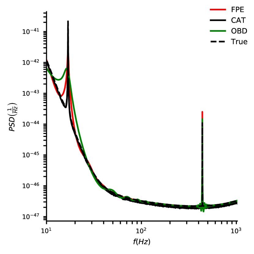
Figure 5: Average spectrum for the three different loss functions as compared with the “true” PSD. The average is computed over $500$ realization of a $40960$ points long time series.

Fig. 5 shows the simulated spectrum (dashed line) and the ensemble-averaged reconstructed PSD adopting the FPE (green line), OBD (red line) and CAT (black line). In all cases, the spectrum is well reconstructed, but with a fairly distinct behaviour at low frequency, where CAT – as in the Gaussian case – better captures and resolves the distinct spectral feature at $\sim$17\text{\,}\mathrm{H}\mathrm{z}$$. In Fig. 7, we report the reconstructed spectra around the two peaks at $\sim$17\text{\,}\mathrm{H}\mathrm{z}$$ and $\sim$438\text{\,}\mathrm{H}\mathrm{z}$$ (left and right panel respectively).

Fig. 6 shows the distribution of recovered AR orders $m$ against the relative frequency-averaged error. The behaviour of the three loss functions is very similar to what found in the Gaussian PSD case (compare it with fig. 4): ODB infers the smallest orders and gives average errors around $20$%, FPE consistently estimates orders of a few hundreds and shows the smallest errors $\sim 15$ % while CAT does not show any preference towards any AR order and displays wildly varying errors. Yet again, when the PSD is averaged over multiple realization of the time, CAT is able to capture the spectrum very precisely. In fact, even in presence of very sharp spectral features, CAT reconstruction seems to be almost perfectly coincident with each of them. Hence, also the study of simulated LIGO data seems to indicate that whenever and wherever ensemble-averaged PSDs are necessary, CAT is the optimal choice of loss function. However, on a single time-series realization, FPE is the more robust choice.

Let us summarize some key general conclusions:

• there are no reasons to prefer OBD over CAT or FPE;

• if we have one single realization for the process, we recommend the use of FPE, that would get the best resolution possible. In this situation, CAT would provide spurious and unreliable results, with large error;

• in the case of several realizations of the same process, CAT ensemble-average properties provide very a precise spectral estimation.

Therefore, the choice of loss function, at least in between CAT and FPE, depends on the problem one is attempting to solve.

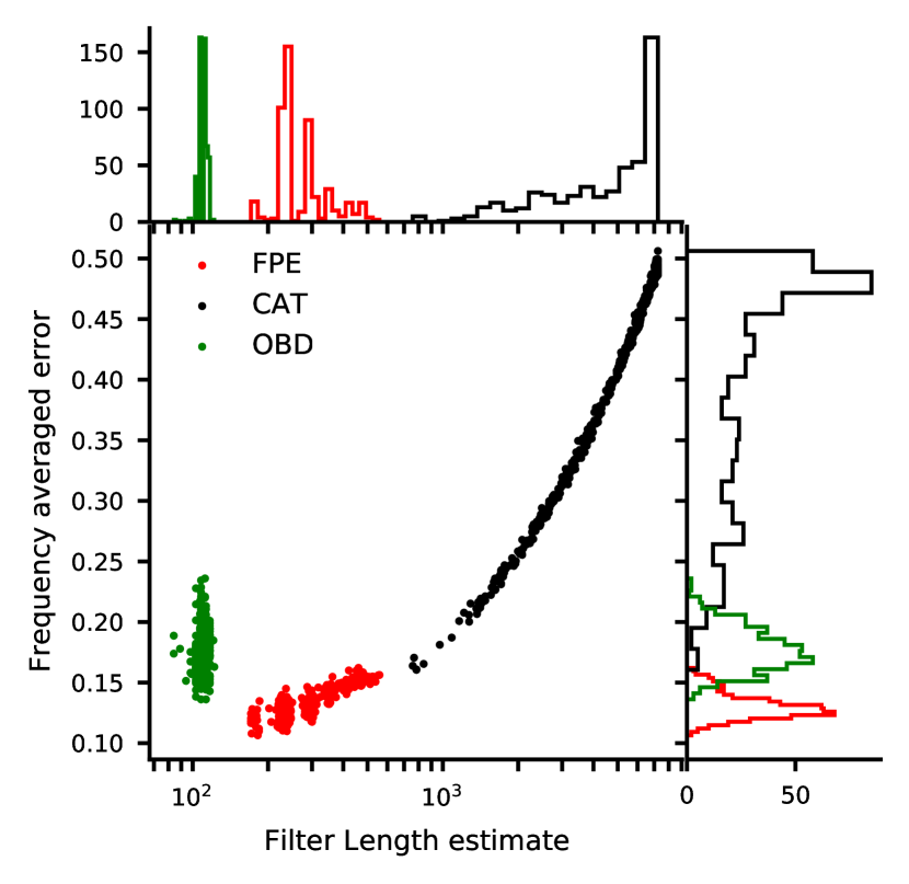
Figure 6: For each of the $500$ independent realization of the time series, we plot the relative error $r$ (as in eq. (24)) against the length $m$ of autoregressive process. The time series are randomly drawn with a the analytical LIGO PSD in fig.‘5. Different colors refers to different choices for the loss function. Histograms for the distribution od the individual quantities are also represented.

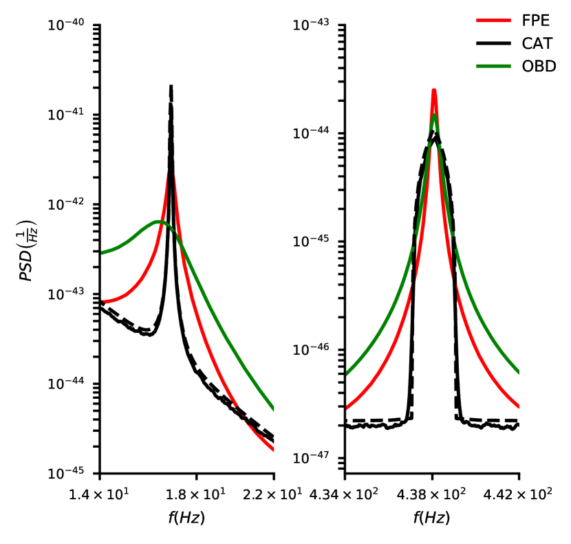
Figure 7: Details of peaks of the spectrum and their reconstruction with every optimizer

3.4 How well is the AR order recovered?

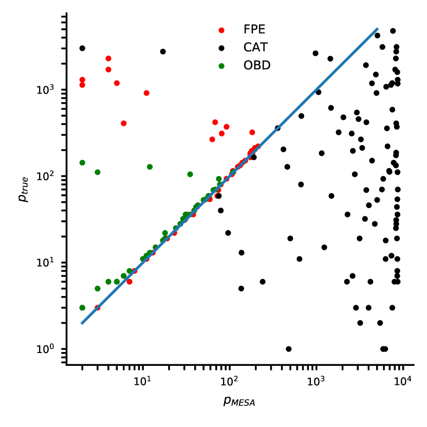
Figure 8: Reconstructed value for the autoregressive order plotted against the true value of the autoregressive order. The reconstructed autoregressive orders are computed from a time series randomly drawn with an $AR(p)$ model, with the three different loss functions under investigation.

We now address the issue of how well the AR order (i.e. the number of $a_{k}$ coefficients employed) is estimated by each loss function. This is useful to further characterize the properties of the different loss functions. Furthermore, as MESA is supposed to model data as an $AR(p)$ process, it is interesting to quantify its precision on some true autoregressive (and stationary) time series.

We generate $100$ autoregressive processes $AR(p)$ with a random value of $p$, drawn such that $log(p)\sim\mathcal{U}_{[log(2),log(5000)]}$. Each coefficient $a_{k}$ is assigned according to a Dirichlet distribution $\mathrm{Dir}([1,\ldots,1])$. The sign of $a_{k}$ is assigned randomly according to a binomial distribution. We report the result of this investigation in Fig. 8.

It can be seen that OBD and FPE loss functions show very similar behaviour. They are very reliable in capturing the correct AR order up to a certain threshold ($p\sim 100$ for OBD and $p\sim 200$ for FPE). For any AR process of order higher than the threshold, the optimization underestimates badly the actual value of $p$. For this reason, FPE and OBD seem reliable only for relatively simple AR processes. For more complicated processes, they seem to “underfit” the problem (i.e. they output a model simpler that those required).

On the other hand, CAT shows a different behaviour. The selected AR order $p$ is always close to the maximum possible value, regardless the actual value $p_{true}$ of the underlying process. This produces always a model that is more complex than those obtained with FPE and OBD and this can explain the origin of the high variance in the estimation observed in the experiments described in the previous sections. Of course, CAT does not perform a good job in reconstructing the AR process. However, for high order AR processes, the error introduced by CAT is more tolerable than the error introduced by FPE and OBD. This is a good reason to prefer CAT in these situations (see also Sec. 5.1 for another example of this effect).

4 Comparison with Welch method

We perform a qualitative comparison between the performance of the MESA and of the standard Welch algorithm. In this, we cannot avoid to be only qualitative. Indeed, as the results of the comparison are problem dependent, it is very hard to quantify this in a single metric. Although similar studies can be drawn from any other PSD, in this section we focus on a single PSD and we try to generalize some observations that we make. We decide to use the analytical PSD computed for LIGO Handford interferometer, released together with the GWCT-1 catalog (Abbott et al. 2019a, b), and computed with BayesLine package (Cornish & Littenberg 2015; Littenberg & Cornish 2015; Cornish et al. 2021; Chatziioannou et al. 2019).

We simulate data from the PSD used for the analysis of the event GW150914 and we employ both Welch’s method and MESA to estimate the spectrum. We vary the length of the data used for the estimation: this is also useful to assess how the computation depends on the data available. We set the total observation time $T=1,5,10,100,1000$\text{\,}\mathrm{s}$$ For the MESA algorithm, we choose the FPE loss function. For the Welch algorithm, we employ a Tukey window with a parameter $\alpha$ equal to 0.4, an overlap fraction of $1/2$ for the segments and a length of segments $L=512,1024,2048,8192,32768$ points, depending on the observation time. In all cases, the sampling rate is set to $4096\text{\,}\mathrm{H}\mathrm{z}$. For the Welch algorithm, we use the standard implementation provided by the python library scipy (Harris et al. 2020; Virtanen et al. 2020). The results from both methods are summarized in Figs. 10 and 10 respectively.

First of all, we note that using a longer time series results in a better estimation of the PSD, especially at low frequencies. This is somehow obvious: longer data streams probe lower frequencies thanks to Nyquist’s theorem as well as providing better estimates for the FFT, in the Welch case, and the sample autocorrelation, for MESA.

We also note that MESA converges to the underlying spectrum much faster than Welch’s method, providing a better estimate even in the case of short time series. Although observed at every frequency, this behaviour is more evident in the low frequency region. An accurate profile reconstruction can be obtained with MESA using a 5 seconds-strain only, while Welch method requires at least 10 seconds of data to obtain a comparable profile. Furthermore, MESA is able to model all the details of the peak at around $\sim$40\text{\,}\mathrm{H}\mathrm{z}$$ (even with $T=$100\text{\,}\mathrm{s}$$), while the Welch’s algorithm fails to do so even with an observation time of $T=$1000\text{\,}\mathrm{s}$$.

Another important element is the noise of the spectral estimation: we find that the PSD estimation provided by the Welch’s method is more noisy (i.e. has a large number of spurious peaks) compared to the PSD measured with MESA and FPE loss function. This is especially true at high frequencies and for long observation times $T$.

Finally, as already discussed Welch’s method is very dependent on the choice of window function. A Tukey window with aforementioned parameters is what we found to be the best compromise between noise and accuracy for the reconstruction, but different choices can be made, possibly providing more accurate results than the ones reported here. However, we want to stress that this fact does not invalidate our discussion but reinforces it: one of the most appealing advantages of MESA is the minimal amount of fine tuning required.

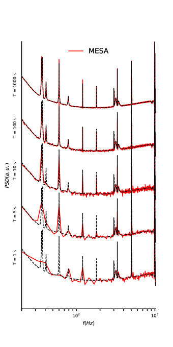
Figure 9: Comparison between analytic (dashed line) and estimated (red line) spectrum. The estimation is performed with Maximum Entropy method on synthetic data, with an increasing observation time $T=1,5,10,100,$1000\text{\,}\mathrm{s}$$.

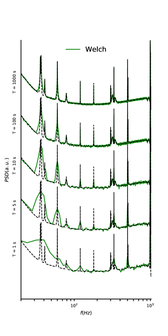
Figure 10: Comparison between analytic (dashed line) and estimated (green line) spectrum. The estimation is performed with Welch’s method on synthetic data with an increasing observation time $T=1,5,10,100,$1000\text{\,}\mathrm{s}$$.

5 Applications

5.1 Temperature Time Series

As a further example of the breadth of applicability of MESA, we applied our implementation to atmospheric temperature time series. The reason for this choice is twofold: i) atmospheric temperature time series present a variety of overlapping periodicities most of which are known; ii) it provides a stress test for the time series forecast analysis. As dataset, we used the historical reanalysis data from the “ERA5-Land hourly data from 1981 to present” dataset, downloaded from the Climate Data Store (Muñoz Sabater 2019). The data consist in temperatures taken at coordinates N $45\mathrm{°}⁤5\mathrm{\prime }$  E $9\mathrm{°}⁤1\mathrm{\prime }$, corresponding about to the city of Milan, Italy. The temperatures are given on an hourly cadence for almost 31 years from 31st December 1989 to 30th November 2020.

Fig. 11, shows the MESA spectrum inferred from the data. As a comparison, we adopt both the FPE and the CAT loss functions. In agreement with what we found in previous sections, the FPE PSD is more regular compared to the one from CAT. Both spectra show a peak at the frequency $f_{D}=$1\text{\,}\mathrm{d}\mathrm{a}\mathrm{y}^{-1}$$ corresponding to one day, corresponding to the day-night cycle: this is expected. Higher order harmonics (corresponding to integer multiples of $f_{D}$) are also visible up to the Nyquist frequency ($f_{D}=$0.5\text{\,}\mathrm{h}\mathrm{o}\mathrm{u}\mathrm{r}^{-1}$$): they correspond to signals that preserve the 1 day period while, at the same time, capturing the complex variability of the daily temperature cycle throughout the year.

Looking at low frequencies, FPE does not capture the yearly variability at $f_{yr}=$1\text{\,}\mathrm{y}\mathrm{r}^{-1}$$. On the other hand, the peak is captured well by the CAT loss function. In analogy as what observed for the peak at $f_{D}$, in the CAT spectrum we observe a higher order harmonic at a frequency $2\cdot f_{yr}$. As in the previous case, this is required to better model the temperature variation in the year.

The failure of FPE in capturing the low frequency trend can be understood by looking at Fig. 8. It is shown that CAT systematically select very long filters (i.e. large $p_{CAT}$ values for the autoregressive orders), whereas FPE tends to select smaller values for the order $p_{FPE}$ of the autoregressive process, often underestimating the actual value. In this example, we have $p_{CAT}\sim 36500\sim$4\text{\,}\mathrm{y}\mathrm{r}$$, whereas $p_{FPE}\sim 1300\sim$2\text{\,}\mathrm{m}\mathrm{o}\mathrm{n}\mathrm{t}\mathrm{h}\mathrm{s}$$. The autoregressive process selected by FPE, hence cannot produce a meaningful prediction on the timescale longer than a few weeks and for this reason it is unable to capture the low frequency peak at $f_{yr}$. In other words, the model is too simple to model both the behaviour at high and low frequencies (separated by approximately 3 orders of magnitude). On the other hand, the model chosen by CAT is much more complex and is able to model also the high frequency behaviour, at the expense of making a more noisy estimation. The “actual” length of the autoregressive process should be closer to the choice of CAT.

We now assess the accuracy of the forecasting of new observations of the time series. Based on actual data, we try to predict future values as described in sec. 2.4 (of course the MESA is performed with CAT loss function). We produce $N=100$ independent predictions and we compute the median as well as the $90\%$ confidence interval. This is compared with the actual measured temperature values. The predictions span a two years range of time. We report our results in Fig. 11.

We note the observed difference is always well included in the $90\%$ confidence interval: the forecasting predictions seem reliable. On the other hand, the confidence interval is pretty large (almost as large as $15\text{\,}\mathrm{K}$), thus making “easy” for the actual data to fit the predictions. Indeed, the prediction model, while suitable for spectral estimation, is nothing more than a linear regression (plus noise term). Such a simple model hardly catches the complex trend in the variability of the temperature daily trend during a year. For more precise predictions, probably one should consider nonlinear regression model, tapping into the wealth of non linear predictors offered by the field of Deep Learning.

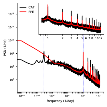
Figure 11: Spectrum for the historical temperature time series. The two lines refers to different loss functions (CAT and FPE); the inset shows the harmonics of the fundamental frequency of a day. Two vertical lines are drawn in correspondence to the frequency $f_{D}$ of a day and $f_{yr}$ of a year.

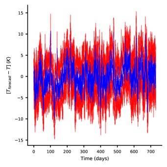
Figure 12: Difference between the historical temperature $T$ and the forecast temperature $T_{forecast}$ for two years of data. The red shadow denotes the $90\%$ confidence interval of the predictions. The model is trained with CAT loss function. The discrepancy between predicted and actual values is always everywhere included in the $90\%$ confidence interval.

5.2 Forecasting the LIGO strain

As a last example of an application of MESA, we return to the study of the strain produced by the LIGO-Virgo interferometers and we forecast the future observations. A seminal work on the application of autoregressive models to Virgo data is presented in Cuoco et al. (2001), where an $AR(p)$ model is trained on the data for the purpose of estimating the PSD and to create a whitener filter.

We focus on the public data released by the LIGO/Virgo collaboration (Abbott et al. 2021). We reconstruct the PSD both assuming the CAT and FPE loss functions on $1000\text{\,}\mathrm{s}$ of data from the Livingston observatory starting from GPS time $1164603392$. The data are sampled at $4096\text{\,}\mathrm{H}\mathrm{z}$. We then forecast the following $100\text{\,}\mathrm{s}$ of observations with the model optimized with CAT. The results are shown in fig. 13. The prediction is always in the $90\%$ confidence interval. The confidence interval, however, is very broad and the prediction is not very accurate (being the same order of magnitude of the strain). By looking at the standard deviation $\sigma$ of the predictions (bottom panel in Fig. 13), we note that it increases very quickly in the first $0.5\text{\,}\mathrm{s}$. The order of the autoregressive process selected is $p_{CAT}=57766\sim$14\text{\,}\mathrm{s}$$, which is much larger than the region in which $\sigma$ is small $\sim$0.2\text{\,}\mathrm{s}$$. The implication is that the series is very difficult to predict: the knowledge of past observations is not very helpful to predict future observations. Although FPE selects an autoregressive order $p_{FPE}=29924\sim$7\text{\,}\mathrm{s}$$ smaller than CAT, the forecasted time series behaves very similarly.

Despite poor predictions on long timescales, the AR process obtained with MESA still can be useful on short timescales. Indeed, a precise prediction of the strain time series can be beneficial in the detection of anomalies in the data and, eventually, their removal. Indeed loud anomalies in the data, called glitches, pose a major challenge to the ability of detecting signals and intensive work has been done to mitigate the disruption in sensitivity they cause (Nuttall et al. 2015; Abbott et al. 2016; Zevin et al. 2017) and to develop effective subraction techniques (Pankow et al. 2018; Zackay et al. 2019). The predictions can form an expected baseline for the strain; any anomaly (i.e. a glitch or even a transient of physical origin) can show up as a large departure from expected trend. Moreover, if a glitch is detected, its shape can be estimated (as well as the confidence level) by subtracting the expected signal with the actual signal. This can work: a typical glitch can last as long as $0.2\text{\,}\mathrm{s}$, close to the time scale over which the forecasting is reliable. Future works will explore this exicting opportunity.

As noted above, for pushing further the prediction performance from our simple linear predictor, more sophisticated forecasting methods are available in the Machine Learning literature (see e.g. (Hochreiter & Schmidhuber 1997; van den Oord et al. 2016; Lea et al. 2016)) and they can be trained for precision forecasting. However, a Maximum-Entropy trained AR process can be a simple baseline for comparing such more advanced methods and might suffice for many purposes. This opens a promising path in GW data analysis and other fields of physics might also take advantage from this.

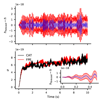
Figure 13: In the top panel, we show the difference between the forecasted strain values (CAT model) and the actual values observed at Livingston interferometer (blue). The red shadow denotes the $90\%$ confidence interval subtracted with the actual time series values. The confidence interval is computed on $100$ independent random realization of the predictions. The bottom panel displays the standard deviation of the predictions with both CAT and FPE models. The inset shows a detail of the first $0.5\text{\,}\mathrm{s}$ of plot in the top panel.

6 Final remarks and future prospects

We presented a case study of the application of Maximum Entropy principle to the realm of spectral estimation. Albeit the methodology hereby presented is grounded on solid theoretical foundations and its merits are widely recognised, Maximum Entropy methods have yet to be adopted routinely in the study of problems related to time series. The superior nature of maximum entropy methods, and in particular of Burg’s method, is exemplified by the closed form estimate of the power spectral density and by the theoretical bridge between spectral analysis and AR processes. Moreover, the method presents, in our view, two main advantages when compared with more traditional ones; first there is no need to choose an arbitrary window function to correct the data and, second it provides as straightforward way to compute predictions given past observations. Accompanying this work, we provide a publicly available Python implementation, called memspectrum, that we used to perform the numerical studies presented in this work..

Since the order of the AR process is not yet determined by the theory, we opted for an in-depth investigation of several proposals in the literature and found that different loss functions are required for different situations, with the FPE loss function being the most indicated to deal with gravitational wave data. Along these lines, we directly compared the PSDs computed with MESA with the canonical Welch’s algorithm. As outlined in Sec. 4, MESA provides PSD estimates with smaller variance and better accuracy than Welch algorithm. The use of MESA is particularly useful for short time series samples, where Welch’s method is outperformed in both precision and confidence.

This observation suggests a promising avenue to pursue in future developments of gravitational waves data analysis: for short time series, comparable with the length of binary black hole systems as observed by LIGO, Virgo and KAGRA, the computational cost of MESA is moderate and the inferred PSD is an accurate representation of the true underlying PSD. Hence MESA could be employed for online PSD estimation during a Bayesian parameter estimation exercise.

This is possible whenever the log-likelihood of the model for a time series takes the form

$$\log\mathcal{L}(d_{t}|\theta)\propto-\frac{1}{2}\frac{|\tilde{d}(f)-\tilde{x}(f;\theta)|^{2}}{S(f)}-\frac{1}{2}\log\left[\int df\,S(f)\right]$$ (26)

where $\tilde{\hphantom{a}}$ denotes the Fourier transform and the signal model $x(t;\theta)$, dependent on some parameter $\theta$, is a prediction for a deterministic signal buried in the observed time series $d(t)$. In GW data analysis, a typical approach is to estimate the PSD offline on a large batch of data and off-source: this scheme assumes stationary data on a long timescale (longer than the data under study) and it might not reflect the structure of the noise in the analyzed time slice. Some alternatives exist for dropping this assumption and modifying the likelihood accordingly (Röver et al. 2010; Röver 2011; Edwards et al. 2020; Chatziioannou et al. 2021). MESA can add to those an elegant way out: at each evaluation of the likelihood, a new spectral analysis is performed by computing the PSD on the residual $d_{t}-x_{t}$. In this way, the PSD would depend also on $\theta$ and would effectively model the residuals. For this method, we would only need to assume the stationariety of the residual on the batch to analyse, making a lighter assumption on the nature of the data. Furthermore, this method would get, as a bonus, a posterior distribution for the PSD of the analyzed data. Preliminary studies suggest that this is possible (Martini 2020). Other studies have been done in this direction, mostly using a parametric model for the PSD (Littenberg et al. 2013; Edwards et al. 2015; Veitch et al. 2015).

Furthermore, MESA provides a simple, but robust and quite accurate, albeit for short times, predictor for the time series. This fact is remarkable and can be used in time series analysis for several purposes. As discussed in Sec. 5.2, an anomaly detection pipeline could be built using the forecasts of MESA: the predictions can form a baseline to compare the actual observations with. Whenever the observed data are outside the expectations, an anomaly detection can be claimed. Of course such predictions can be done with a more accurate (perhaps nonlinear) model; however MESA has the advantage of being simple and fast to construct, while providing decent predictions. At the same time, several instruments present gaps in their data stream, for instance LISA is expected to show such gaps (e.g. Baghi et al. (2019) and references therein), MESA forecasting capabilities could be used to fill those gaps with predicted data from past observations. In conclusion, we reiterate that MESA is a theoretically sound, computationally feasible and reliable way of studying the properties of stochastic processes and we hope that the investigations presented in this work will further stimulate developments and applications of this method.

Acknowledgments

We are grateful to S. Biscoveanu, D. Laghi, M. Maugeri, C. Rossi and S. Shore for useful comments and discussions.
This research has made use of data, software and/or web tools obtained from the Gravitational Wave Open Science Center (https://www.gw-openscience.org/), a service of LIGO Laboratory, the LIGO Scientific Collaboration and the Virgo Collaboration. LIGO Laboratory and Advanced LIGO are funded by the United States National Science Foundation (NSF) as well as the Science and Technology Facilities Council (STFC) of the United Kingdom, the Max-Planck-Society (MPS), and the State of Niedersachsen/Germany for support of the construction of Advanced LIGO and construction and operation of the GEO600 detector. Additional support for Advanced LIGO was provided by the Australian Research Council. Virgo is funded, through the European Gravitational Observatory (EGO), by the French Centre National de Recherche Scientifique (CNRS), the Italian Istituto Nazionale di Fisica Nucleare (INFN) and the Dutch Nikhef, with contributions by institutions from Belgium, Germany, Greece, Hungary, Ireland, Japan, Monaco, Poland, Portugal, Spain.

Appendix A Details of PSD computation

A.1 MESA solution

We derive the expression for the MAXENT spectral estimator following the approach proposed by Burg (1975). Unlike the standard approach, we do not enforce the constraints in Eq. (11) with the standard Lagrange Multipliers approach. We write instead the PSD $S(f)$ as the Fourier Transform of the sample autocorrelation function:

$$S(f)=\frac{1}{2Ny}\sum_{n=-\infty}^{\infty}\bar{r}_{n}e^{-\imath 2\pi n\Delta t},$$ (27)

and, plugging it in the entropy gain expression eq. (10), we obtain:

$$\Delta H=\int_{-Ny}^{Ny}\log\left(\frac{1}{2Ny}\sum_{n=-\infty}^{\infty}\bar{r}_{n}e^{-\imath 2\pi fn\Delta t}\right)df.$$ (28)

Note that this expression already takes into account the constraints in eq. (11).

We now introduce a set of coefficients $\lambda_{s}$, defined as the derivative of $\Delta H$ with respect to the autocorrelation function $r_{s}$. Explicitly they are:

$$\lambda_{s}\coloneqq\frac{\delta H}{\delta\bar{r}_{s}}=\frac{1}{2Ny}\int_{-Ny}^{Ny}S(f)^{-1}e^{-\imath 2\pi fs\Delta t}df$$ (29)

and we will show that $S(f)^{-1}$ can be written as a Fourier Expansion in terms of such coefficients. Then, the determination of the values for the $\lambda_{s}$ uniquely solves the problem of power-spectral density estimation.

Some properties for the coefficients can be worked out easily. First, since $S(f)$ is real, the $\lambda_{s}$ show the property

$$\lambda_{s}=\lambda_{-s}^{*}.$$

The second property is obtained considering that the autocorrelation function $r_{n}$ can only be computed for a finite time interval $n\in[-N,N]$ and that the PSD estimation must not depend on the unavailable values $r_{n}$: this is part of the constraint in eq. (11) This requirement can be implemented as:

$$\frac{\delta H}{\delta\bar{r}_{s}}=0\text{ for }|s|>N,$$

that means

$$\lambda_{s}=0\text{ for }|s|>N.$$

From Eq. (29) and from the properties above, is easily seen from the properties of the Fourier transform that $S(f)$ can be expressed via a Fourier Series

$$S(f)^{-1}=\sum_{s=-N}^{N}\lambda_{s}e^{-\imath 2\pi fs\Delta t}.$$ (30)

Defining $z=e^{-\imath 2\pi f\Delta t}$ the previous Fourier expansion becomes a Laurent Polynomial in $z$:

$$S(f)^{-1}=\lambda_{0}+\sum_{s=1}^{N}\lambda_{s}z^{s}+\sum_{s=1}^{N}\lambda^{*}_{s}z^{-s}.$$ (31)

It is easy to show that if $z_{0}$ is a root for the polynomial $(z_{0}^{*})^{-1}$ is also a root: for every root laying outside the unit circle there will be another root inside of it and vice-versa. These properties allow us to rewrite the Fourier expansion (31) as (Barnard 1975):

$$S(f)=\frac{P_{N}\Delta t}{\left(\sum_{s=0}^{N}a_{s}z^{z}\right)\left(\sum_{s=0}^{N}a^{*}_{s}z^{-s}\right)}$$ (32)

with $a_{0}=1$ and $\Delta t$ the uniform sampling interval for the time series. The vector obtained as $(1,a_{1},\dots,a_{N})$ is the prediction error filter. The power spectral density $S(f)$ is uniquely determined if both the prediction error filter and $P_{N}$ coefficients are computed.

To compute the $a_{s}$ is convenient to plug into Eq. (11) the Laurent Polynomial exansion for $S(f)$ eq. (32) and then integrating over $z$ (taking values on ${\mathbb{S}^{1}}$). In this way the equation becomes:

$$\frac{P_{N}}{2\pi\imath}\oint_{\mathbb{S}^{1}}\frac{z^{-s-1}}{\sum_{n=0}^{N}a_{n}z^{n}\sum_{n=0}^{N}a^{*}_{n}z^{-n}}dz=\bar{r}_{s}.$$ (33)

Substituting $s\to s-r$, multiplying by $a^{*}_{s}$ and summing over $s$, the previous equation becomes

$$\sum_{s=0}^{N}a_{s}\bar{r}_{s-r}=\frac{P_{N}}{2\pi\imath}\oint\frac{z^{r-1}}{\sum_{s=0}^{N}a_{s}z^{s}}dz$$ (34)

For a wide-sense stationary processes, all the poles lay outside the unit circle so that the previous integral can be easily computed obtaining the following, well known, equations:

$$\sum_{s=0}^{N}a_{s}\bar{r}_{r-s} =P_{N}\quad\text{ if }r=0$$ (35)

$$\sum_{s=0}^{N}a_{s}\bar{r}_{r-s} =0\qquad\text{ if }r\neq 0.$$ (36)

A.2 Levinson recursion

The solution of the Eqs. (35-36) fully determines the functional form of the power spectral density estimator (32). The method for solving the equations is called the Levinson-Durbin recursion (Levinson 1946) and it is described in the following. For each order $N$ of the iteration we define the quantities:

$$\Delta_{N} =\sum_{n=0}^{N}a_{n}\bar{r}_{N-n+1}$$ (37)

$$c_{N} =-\frac{\Delta_{N}}{P_{N}},$$ (38)

The Levinson recursion computes the $N$th order quantities given the $N-1$th order quantities:

$$P_{N}=P_{N-1}\left(1-|c_{N-1}|^{2}\right)$$ (39)

and

$$\begin{pmatrix}1\\ a_{1}\\ \vdots\\ a_{N-1}\\ a_{N}\end{pmatrix}=\begin{pmatrix}1\\ b_{1}\\ \vdots\\ b_{N-1}\\ 0\end{pmatrix}+c_{N-1}\begin{pmatrix}0\\ b_{N-1}^{*}\\ \vdots\\ b^{*}_{1}\\ 1\end{pmatrix}.$$ (40)

where $b$ holds the value of the $a_{s}$ coefficients at order $N-1$. The 0-th order element can be easily initialized reminding that $a_{0}=1$ (always) and that $P_{0}$ can be determined from (35). Its values turns out to be:

$$P_{0}=R(0),$$ (41)

$\Delta_{0}$ and $c_{0}$ are uniquely determined from their definitions and they are:

$$\Delta_{0}=R(1);\quad c_{0}=-\frac{R(1)}{R(0)}.$$ (42)

These expressions allow us to compute $\@vec{a}$ and $P_{N}$ to any order by simply iterating (39) and (40). Substituting them in equation (32) the problem of the estimation for the power spectral density via maximum entropy principle is solved. Burg’s method for spectral analysis is solved via Levinson is implemented in the released memspectrum package. Another faster recursion method is available in Vos (2013) and it is also available in memspectrum.

References

- Aasi et al. (2015) Aasi, J., Abbott, B. P., Abbott, R., et al. 2015, Classical and Quantum Gravity, 32, 074001
- Abbott et al. (2019a) Abbott, B., Abbott, R., Abbott, T., et al. 2019a, Physical Review X, 9
- Abbott et al. (2019b) Abbott, B., Abbott, R., Abbott, T., et al. 2019b, LIGO Document P1900011-Power Spectral Densities (PSD) release for GWTC-1, LIGO Document Service: https://dcc.ligo.org/LIGO-P1900011/public
- Abbott et al. (2016) Abbott, B. P., Abbott, R., Abbott, T. D., et al. 2016, Classical and Quantum Gravity, 33, 134001
- Abbott et al. (2020) Abbott, B. P., Abbott, R., Abbott, T. D., et al. 2020, Living Reviews in Relativity, 23
- Abbott et al. (2021) Abbott, R., Abbott, T., Abraham, S., et al. 2021, SoftwareX, 13, 100658
- Ables (1974) Ables, J. G. 1974, Astronomy and Astrophysics Supplement, 15, 383
- Acernese et al. (2014) Acernese, F., Agathos, M., Agatsuma, K., et al. 2014, Classical and Quantum Gravity, 32, 024001
- Akaike (1998) Akaike, H. 1998, Annals of the Institute of Statistical Mathematics, 137
- Allen et al. (2012) Allen, B., Anderson, W. G., Brady, P. R., Brown, D. A., & Creighton, J. D. E. 2012, Phys. Rev. D, 85, 122006
- Aso et al. (2013) Aso, Y., Michimura, Y., Somiya, K., et al. 2013, Physical Review D, 88
- Baghi et al. (2019) Baghi, Q., Thorpe, J. I., Slutsky, J., et al. 2019, Phys. Rev. D, 100, 022003
- Barnard (1975) Barnard, T. E. 1975, The maximum entropy spectrum and the Burg technique. Technical report no. 1: Advanced signal processing, NASA STI/Recon Technical Report N
- Bartlett (1968) Bartlett, M. 1968, Louvain Economic Review, 34, 227–227
- Berryman (1978) Berryman, J. G. 1978, GEOPHYSICS, 43, 1384
- Bhansali (1986) Bhansali, R. J. 1986, Annals of Statistics., 14, 315
- Biscoveanu et al. (2020) Biscoveanu, S., Haster, C.-J., Vitale, S., & Davies, J. 2020, Physical Review D, 102
- Burg (1975) Burg, J. 1975, Maximum Entropy Spectral Analysis, Stanford Exploration Project (Stanford University)
- Chatziioannou et al. (2021) Chatziioannou, K., Cornish, N., Wijngaarden, M., & Littenberg, T. B. 2021, Physical Review D, 103
- Chatziioannou et al. (2019) Chatziioannou, K., Haster, C.-J., Littenberg, T. B., et al. 2019, Physical Review D, 100
- Cornish & Littenberg (2015) Cornish, N. J. & Littenberg, T. B. 2015, Classical and Quantum Gravity, 32, 135012
- Cornish et al. (2021) Cornish, N. J., Littenberg, T. B., Bécsy, B., et al. 2021, Phys. Rev. D, 103, 044006
- Cuoco et al. (2001) Cuoco, E., Calamai, G., Fabbroni, L., et al. 2001, Classical and Quantum Gravity, 18, 1727–1751
- Edwards et al. (2020) Edwards, M. C., Maturana-Russel, P., Meyer, R., et al. 2020, Physical Review D, 102
- Edwards et al. (2015) Edwards, M. C., Meyer, R., & Christensen, N. 2015, Physical Review D, 92
- Finn (1992) Finn, L. S. 1992, Physical Review D, 46, 5236–5249
- Gray (2006) Gray, R. M. 2006, Toeplitz and Circulant Matrices: A Review (Now Foundations and Trends)
- Gregory (2005) Gregory, P. 2005, Multivariate Gaussian from maximum entropy (Cambridge University Press), 450–454
- Harris et al. (2020) Harris, C. R., Millman, K. J., van der Walt, S. J., et al. 2020, Nature, 585, 357–362
- Hochreiter & Schmidhuber (1997) Hochreiter, S. & Schmidhuber, J. 1997, Neural computation, 9, 1735
- Jaynes & Bretthorst (2003) Jaynes, E. & Bretthorst, G. 2003, Probability Theory: The Logic of Science (Cambridge University Press:)
- Jaynes (1957) Jaynes, E. T. 1957, Physical Review, 106, 620
- Jaynes (1982) Jaynes, E. T. 1982, Proceedings of the IEEE, 70, 939
- Lea et al. (2016) Lea, C., Flynn, M. D., Vidal, R., Reiter, A., & Hager, G. D. 2016, Temporal Convolutional Networks for Action Segmentation and Detection
- Levinson (1946) Levinson, N. 1946, Journal of Mathematics and Physics, 25, 261
- LIGO/Virgo Collaboration (2020) LIGO/Virgo Collaboration. 2020, Noise curves used for Simulations in the update of the Observing Scenarios Paper, https://dcc.ligo.org/LIGO-T2000012/public
- Littenberg & Cornish (2015) Littenberg, T. B. & Cornish, N. J. 2015, Physical Review D, 91
- Littenberg et al. (2013) Littenberg, T. B., Coughlin, M., Farr, B., & Farr, W. M. 2013, Physical Review D, 88
- Lomb (1976) Lomb, N. R. 1976, Astrophysics and Space Science, 39, 447
- Martini (2020) Martini, A. 2020, Maximum Entropy Spectral Analysis: characterization and applications to on-source parameter estimation of time series, https://etd.adm.unipi.it/theses/available/etd-11162020-182406/
- Muñoz Sabater (2019) Muñoz Sabater, J. 2019, ERA5-Land hourly data from 1981 to present, Copernicus Climate Change Service (C3S) Climate Data Store (CDS): https://cds.climate.copernicus.eu/cdsapp#!/dataset/reanalysis-era5-land
- Nuttall et al. (2015) Nuttall, L. K., Massinger, T. J., Areeda, J., et al. 2015, Classical and Quantum Gravity, 32, 245005
- P. M. Woodward & Higinbotham (1964) P. M. Woodward, D. W. F. & Higinbotham, W. 1964, Probability and information theory, with applications to radar, 2nd edn. (Pergamon Press)
- Pankow et al. (2018) Pankow, C., Chatziioannou, K., Chase, E. A., et al. 2018, Physical Review D, 98
- Rao et al. (1982) Rao, A. R., Kashyap, R. L., & Mao, L. 1982, Water Resources Research, 18, 1097
- Röver (2011) Röver, C. 2011, Physical Review D, 84
- Röver et al. (2010) Röver, C., Meyer, R., & Christensen, N. 2010, Classical and Quantum Gravity, 28, 015010
- Scargle (1982) Scargle, J. D. 1982, The Astrophysical Journal, 263, 835
- Shannon (1948) Shannon, C. E. 1948, Bell System Technical Journal, 27, 379
- Somiya (2012) Somiya, K. 2012, Classical and Quantum Gravity, 29, 124007
- Talbot & Thrane (2020) Talbot, C. & Thrane, E. 2020, Gravitational-wave astronomy with an uncertain noise power spectral density
- Ulrych & Bishop (1975) Ulrych, T. J. & Bishop, T. N. 1975, Reviews of Geophysics, 13, 183
- van den Oord et al. (2016) van den Oord, A., Dieleman, S., Zen, H., et al. 2016, WaveNet: A Generative Model for Raw Audio
- Veitch et al. (2015) Veitch, J., Raymond, V., Farr, B., et al. 2015, Phys. Rev. D, 91, 042003
- Virtanen et al. (2020) Virtanen, P., Gommers, R., Oliphant, T. E., et al. 2020, Nature Methods, 17, 261
- Vos (2013) Vos, K. 2013, A Fast Implementation of Burg’s Algorithm, https://opus-codec.org/docs/vos_fastburg.pdf
- Welch (1967) Welch, P. 1967, IEEE Transactions on audio and electroacoustics, 15, 70
- Wold (1939) Wold, H. 1939, Journal of the Institute of Actuaries, 70, 113–115
- Zackay et al. (2019) Zackay, B., Venumadhav, T., Roulet, J., Dai, L., & Zaldarriaga, M. 2019, Detecting Gravitational Waves in Data with Non-Gaussian Noise
- Zevin et al. (2017) Zevin, M., Coughlin, S., Bahaadini, S., et al. 2017, Classical and Quantum Gravity, 34, 064003