Calculation of force and torque between two arbitrarily oriented circular filaments using Kalantarov-Zeitlin’s method

Abstract

In this article, formulas for calculation of force and torque between two circular filaments arbitrarily oriented in space were derived by using Kalantarov-Zeitlin’s method. Formulas are presented in an analytical form through integral expressions, whose kernel function is expressed in terms of the elliptic integrals of the first and second kinds, and provide an alternative formulation to Babič’s expressions. The derived new formulas were validated via comparison with a series of reference examples. Also, we obtained additional expressions for calculation of force and torque between two circular filaments by means of differentiation of Grover’s formula for the mutual inductance between two circular filaments with respect to appropriate coordinates. These additional expressions allow to verifying comprehensively and independently derived new formulas.

1 Introduction

Analytical and semi-analytical methods in the calculation of parameters of electrical circuits and force interaction between their elements play an important role in power transfer, wireless communication, and sensing and actuation, and are applied in different fields of science, including electrical and electronic engineering, medicine, physics, nuclear magnetic resonance, mechatronics and robotics, to name the most prominent. A number of efficient numerical methods implemented in the commercially available software currently provides an accurate and fast solution for the calculation of parameters of electrical circuits. However, analytical methods allow to obtain the result in the form of a final formula with a finite number of input parameters, which when applicable may significantly reduce computation effort. It will also facilitate mathematical analysis, for example, when derivatives of the mutual inductance with respect to one or more parameters are required to evaluate electromagnetic forces via the stored magnetic energy, or when optimization is performed.

Analytical methods applied to the calculation of force and torque between two circular filaments, which is closely related to calculation of the mutual inductance in such the system, is a prime example. These methods have been successfully used in an increasing number of applications, including electromagnetic levitation [1], superconducting levitation [2, 3, 4], magnetic force interaction [5], wireless power transfer [6, 7, 8], electromagnetic actuation [9, 10, 11, 12], micro-machined contactless inductive suspensions [13, 14, 15, 16, 17] and hybrid suspensions [18, 19, 20, 21], biomedical applications [22, 23], topology optimization [24], nuclear magnetic resonance [25, 26], indoor positioning systems [27], navigation sensors [28], wireless power transfer systems [29] and magneto-inductive wireless communications [30].

The calculation of force and torque between two circular filaments with running electrical current is reduced to finding first derivatives of a function of mutual inductance corresponding to this filament system. In 1954, using the mutual inductance between two coaxial circular filaments derived by Maxwell [31, page 340, Art. 701], C. Snow obtained the formula for calculation attractive force between them in work [32]. Also, in the same work [32] C. Snow presented formulas for calculation of torque between circular filaments covering the following cases, namely, when axes of circular filaments are intersected, and two concentric circles, and for calculation of force between two parallel circles. The formulas were expressed via series over the Legendre polynomials. In 1996, Kim et al. developed the expression for calculation of the restoring force in a system of two non-coaxial coils based on magnetic potential method [33]. Employing Grover’s formula for calculation of mutual inductance between two filament coils [34], Babič et al. developed the formulas for calculation of force and torque in such filament coil systems, in which circles have the lateral misalignment [35] and whose ases are inclined at the same plane [36, 37], respectively. The developed formulas were applied to the calculation of force interaction between superconducting magnets and coils having a rectangular cross-section. In work [38], Babič et al. presented new general formulas for calculating the magnetic force between inclined circular filaments placed in any desired position based on two approaches, namely, Biot-Savart’s law and the formula for calculation of the mutual inductance [39].

In this article, new formulas for calculation of force and torque between two circular filaments arbitrarily oriented in space presented in an integral analytical form, whose kernel function is expressed in terms of the elliptic integrals of the first and second kinds, were derived based on Kalantarov-Zeitlin’s method and provide an alternative formulation to Babič’s expressions. Kalantarov and Zeitlin showed that the calculation of mutual inductance between a circular primary filament and any other secondary filament having an arbitrary shape and any desired position with respect to the primary filament can be reduced to a line integral [40, Sec. 1-12, page 49]. Adapting this method to the case of two circular filaments, the author derived analytical formulas for calculating the mutual inductance between two circular filaments having any desired position with respect to each other in work [41]. Taking first derivatives with respect to the appropriate coordinates of the formulas for calculation of the mutual inductance obtained by means of Kalantarov-Zeitlin’s method, the derivation of these presented formulas for calculation of force and torque was carried out.

Developed new formulas were successfully verified by the examples taken from Babič et al. work [38] and comparison with results of calculation of force and torque performed by expressions derived from Grover’s formula for calculation of mutual inductance [42, page 207, Eq. (179)]. For the convenience of a reader, all derived formulas including expressions derived by Grover’s method were programmed by using the Matlab language. The Matlab files with the implemented formulas are available from the author as supplementary materials to this article.

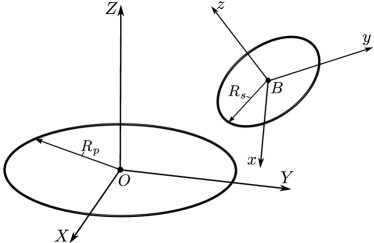
Figure 1: General scheme of arbitrarily positioning two circular filaments with respect to each other.

2 Preliminary discussion

Similar to our previous work [41], the general scheme of arbitrarily positioning of two circular filaments with respect to each other is considered as shown in Fig. 1. The primary circular filament (the primary circle) and the secondary circular filament (the secondary circle) have radii of $R_{p}$ and $R_{s}$, respectively. A coordinate frame (CF) denoted as $XYZ$ is assigned to the primary circle in such a way that the $Z$ axis is coincident with the circle axis and the $XOY$ plane of the CF lies on circle’s plane, where the origin $O$ corresponds to the centre of primary circle. In turn, the $xyz$ CF is assigned to the secondary circle in a similar way so that its origin $B$ is coincident with the centre of the secondary circle.

The linear misalignment of the secondary circle with respect to the primary one is defined by the coordinates of the centre $B$ ($x_{B},y_{B},z_{B}$). The angular misalignment of the secondary circle can be defined by using Grover’s angles [42, page 207]. Namely, the angle of $\theta$ and $\eta$ corresponds to the angular rotation around an axis passing through the diameter of the secondary circle, and then the rotation of this axis lying on the surface $x^{\prime}By^{\prime}$ around the vertical $z^{\prime}$ axis, respectively, as it is shown in Figure 2(a). As an alternative manner to Grover’s angles, the same angular misalignment can be determined through the $\alpha$ and $\beta$ angle, which corresponds to the angular rotation around the $x^{\prime}$ axis and then around the $y^{\prime\prime}$ axis, respectively, as it is shown in Figure 2(b). This additional second manner is more convenient in a case of study dynamics and stability issues, for instance, applying to axially symmetric inductive levitation systems [14, 16] in compared with Grover’s manner. These two pairs of angles have the following relationship with respect to each other such as [41]:

$$\left\{\begin{array}[]{l}\sin\beta=\sin\eta\sin\theta;\\ \cos\beta\sin\alpha=\cos\eta\sin\theta.\end{array}\right.$$ (1)

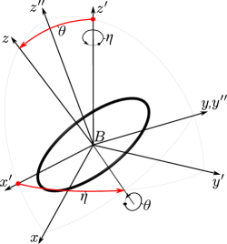
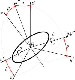
(a)

Figure 2: Two manners for determining the angular position of the secondary circle with respect to the primary one: $x^{\prime}y^{\prime}z^{\prime}$ is the auxiliary CF the axes of which are parallel to the axes of $XYZ$, respectively; $x^{\prime\prime}y^{\prime\prime}z^{\prime\prime}$ is the auxiliary CF defined in such a way that the $x^{\prime}$ and $x^{\prime\prime}$ are coincide, but the $z^{\prime\prime}$ and $y^{\prime\prime}$ axis is rotated by the $\alpha$ angle with respect to the $z^{\prime}$ and $y^{\prime}$ axis, respectively.

The mutual inductance between these two filaments can be calculated by the following formulas, which were derived by using Kalantarov-Zeitlin’s approach in work [41] for two cases. Introducing the following dimensionless coordinates:

$${\displaystyle{x}=\frac{x_{B}}{R_{s}};\;{y}=\frac{y_{B}}{R_{s}};\;{z}=\frac{z_{B}}{R_{s}};{s}=\sqrt{{x}^{2}+{y}^{2}},}\\$$ (2)

for the first case when the $\theta$ angle is lying in interval of $0\leq\theta<\pi/2$, the formula can be written as

$$M=\frac{\mu_{0}\sqrt{R_{p}R_{s}}}{\pi}\int_{0}^{2\pi}{r}\cdot U\cdot\Phi(k)d\varphi,$$ (3)

where

$${r}={r}(\theta,\eta)=\frac{\cos\theta}{\sqrt{\sin^{2}(\varphi-\eta)+\cos^{2}\theta\cos^{2}(\varphi-\eta)}},$$ (4)

$$U=U({x},{y},\theta,\eta)=\frac{R}{{\rho}^{1.5}}=\frac{{r}+t_{1}\cdot\cos\varphi+t_{2}\cdot\sin\varphi}{{\rho}^{1.5}},$$ (5)

$$\begin{array}[]{l}t_{1}=t_{1}({x},{y},\theta,\eta)={x}+0.5\bar{r}^{2}\tan^{2}\theta\sin(2(\varphi-\eta))\cdot{y},\\ t_{2}=t_{2}({x},{y},\theta,\eta)={y}-0.5\bar{r}^{2}\tan^{2}\theta\sin(2(\varphi-\eta))\cdot{x},\\ {\rho}={\rho}({x},{y},\theta,\eta)=\sqrt{{r}^{2}+2{r}\cdot\left({x}\cos(\varphi)+{y}\sin(\varphi)\right)+{s}^{2}},\end{array}$$ (6)

$$\Phi(k)=\frac{1}{k}\left[\left(1-\frac{k^{2}}{2}\right)K(k)-E(k)\right],$$ (7)

and $K(k)$ and $E(k)$ are the complete elliptic functions of the first and second kind, respectively, and

$$\begin{array}[]{l}{\displaystyle k^{2}=k^{2}({x},{y},{z},\theta,\eta)=\frac{4\nu{\rho}}{(\nu{\rho}+1)^{2}+\nu^{2}{z}_{\lambda}^{2}},}\\ {\displaystyle\nu=R_{s}/R_{p},\;{z}_{\lambda}={z}+{r}\tan\theta\sin(\varphi-\eta)}.\end{array}$$ (8)

For the second case when the $\theta$ angle is equal to $\pi/2$ and the two filament circles are mutually perpendicular to each other, the formula becomes

$$\begin{array}[]{l}{\displaystyle M=\frac{\mu_{0}\sqrt{R_{p}R_{s}}}{\pi}\left\{\int_{-1}^{1}U\cdot\Phi(k)d\bar{\ell}\right.}\\ {\displaystyle\left.+\int_{1}^{-1}U\cdot\Phi(k)d\bar{\ell}\right\}},\end{array}$$ (9)

where

$$U=U({x},{y},\eta)=\frac{R}{{\rho}^{1.5}}=\frac{t_{1}-t_{2}}{{\rho}^{1.5}},$$ (10)

$$\begin{array}[]{l}t_{1}=t_{1}({x},\eta)=\sin\eta\cdot({x}+\bar{\ell}\cos\eta),\\ t_{2}=t_{2}({y},\eta)=\cos\eta\cdot({y}+\bar{\ell}\sin\eta),\\ {\rho}={\rho}({x},{y},\eta)=\sqrt{{s}^{2}+2\bar{\ell}\cdot\left({x}\cos(\eta)+{y}\sin(\eta)\right)+\bar{\ell}^{2}},\end{array}$$ (11)

and $\bar{\ell}=\ell/R_{s}$ is the dimensionless variable. The functions $\Phi(k)$ and $k=k({x},{y},{z},\eta)$ in formula (9) have the same structures as defined by Eq. (7) and (8), respectively. Besides that, in the elliptic module $k=k({x},{y},{z},\eta)$, the ${z}_{\lambda}$ function is governed as follows

$${z}_{\lambda}={z}\pm\sqrt{1-\bar{\ell}^{2}},$$ (12)

Note that integrating formula (9) between $-1$ and $1$, Eq. (12) is calculated with the positive sign and for the other direction the negative sign is taken.

Assuming that the primary and secondary circular filaments carry the currents of $I_{p}$ and $I_{s}$, respectively, hence, the magnetic force and torque between these two circular filaments can be calculated by taking the first derivatives of the function of the magnetic energy stored in such the system with respect to the appropriate coordinates. Hence, force can be calculated by

$${\displaystyle F_{g}=I_{p}I_{s}\frac{\partial M}{\partial g},}$$ (13)

where $g=x_{B}$, $y_{B}$, or $z_{B}$. For torque, we can write:

$${\displaystyle T_{g}=I_{p}I_{s}\frac{\partial M}{\partial g},}$$ (14)

where $g=\theta$ or $\eta$. Thus, to derive formulas for calculation of force and torque between two arbitrarily oriented circular filaments, the first derivatives of formulas of mutual inductance, namely, represented by Eq. (3) and (9) must be taken.

3 Derivation of Formulas

In this section the first derivatives of mutual inductance with respect to appropriate coordinates are taken for the two considered above cases separately.

3.1 The first case: $0\leq\theta<\pi/2$

For this case, formula (3) for calculation of mutual inductance is considered. Its kernel is defined as

$$\mathrm{Kr}={r}\cdot U\cdot\Phi(k).$$ (15)

Finding the first derivatives of mutual inductance (3) is reduced to taking the derivatives of kernel function. Following this, firstly five derivatives of the kernel with respect to the defined five coordinates are obtained as follows.

According to the definitions of functions $r$, $U$, $\Phi(k)$ and $k$ given in Eq. (4), (5), (7) and (8), respectively, the $x_{B}$-derivative of kernel $\mathrm{Kr}$ can be written as

$${\displaystyle\frac{\partial\mathrm{Kr}}{\partial x_{B}}=\frac{\partial\mathrm{Kr}}{\partial x}\frac{1}{R_{s}}=\frac{r}{R_{s}}\cdot\left[\frac{\partial U}{\partial x}\cdot\Phi(k)+U\cdot\frac{d\Phi(k)}{dk}\cdot\frac{\partial k}{\partial x}\right],}$$ (16)

where

$$\begin{array}[]{l}{\displaystyle\frac{\partial U}{\partial x}=\left({\displaystyle\frac{\partial R}{\partial x}}\cdot\rho-1.5\cdot R\cdot\frac{\partial\rho}{\partial x}\right)\bigg{/}{{\rho}^{2.5}},}\\ {\displaystyle\frac{\partial R}{\partial x}=\frac{\partial t_{1}}{\partial x}\cdot\cos\varphi+\frac{\partial t_{2}}{\partial x}\cdot\sin\varphi},\\ {\displaystyle\frac{\partial t_{1}}{\partial x}=1,\;\frac{\partial t_{2}}{\partial x}=-0.5\bar{r}^{2}\tan^{2}\theta\sin(2(\varphi-\eta))},\\ {\displaystyle\frac{\partial\rho}{\partial x}=\left(r\cdot\cos\varphi+x\right)\big{/}{{\rho}},}\end{array}$$ (17)

$$\frac{d\Phi(k)}{dk}=\frac{1}{k^{2}}\left[\frac{2-k^{2}}{2(1-k^{2})}E(k)-K(k)\right],$$ (18)

$${\displaystyle\frac{\partial k}{\partial x}=\frac{2/k-k(\nu{\rho}+1)}{(\nu{\rho}+1)^{2}+\nu^{2}{z}_{\lambda}^{2}}\cdot\nu\frac{\partial\rho}{\partial x}.}$$ (19)

For the $y_{B}$-derivative of kernel $\mathrm{Kr}$, we have

$${\displaystyle\frac{\partial\mathrm{Kr}}{\partial y_{B}}=\frac{\partial\mathrm{Kr}}{\partial y}\frac{1}{R_{s}}=\frac{r}{R_{s}}\cdot\left[\frac{\partial U}{\partial y}\cdot\Phi(k)+U\cdot\frac{d\Phi(k)}{dk}\cdot\frac{\partial k}{\partial y}\right],}$$ (20)

where

$$\begin{array}[]{l}{\displaystyle\frac{\partial U}{\partial y}=\left({\displaystyle\frac{\partial R}{\partial y}}\cdot\rho-1.5\cdot R\cdot\frac{\partial\rho}{\partial y}\right)\bigg{/}{{\rho}^{2.5}},}\\ {\displaystyle\frac{\partial R}{\partial y}=\frac{\partial t_{1}}{\partial y}\cdot\cos\varphi+\frac{\partial t_{2}}{\partial y}\cdot\sin\varphi},\\ {\displaystyle\frac{\partial t_{1}}{\partial y}=0.5\bar{r}^{2}\tan^{2}\theta\sin(2(\varphi-\eta)),\;\frac{\partial t_{2}}{\partial y}=1},\\ {\displaystyle\frac{\partial\rho}{\partial y}=\left(r\cdot\sin\varphi+y\right)\big{/}{{\rho}}.}\end{array}$$ (21)

The derivative of elliptic module $k$ with respect to $y$ has a similar form to Eq. (19), but in the later one the partial derivative, ${\displaystyle\frac{\partial\rho}{\partial x}}$, must be replaced by ${\displaystyle\frac{\partial\rho}{\partial y}}$ defined in (21). The $z_{B}$-derivative of kernel $\mathrm{Kr}$ is

$${\displaystyle\frac{\partial\mathrm{Kr}}{\partial z_{B}}=\frac{\partial\mathrm{Kr}}{\partial z}\frac{1}{R_{s}}=\frac{r}{R_{s}}\cdot U\cdot\frac{d\Phi(k)}{dk}\cdot\frac{\partial k}{\partial z},}$$ (22)

where

$${\displaystyle\frac{\partial k}{\partial z}=-\sqrt{4\nu\rho}\cdot\frac{\nu^{2}{z}_{\lambda}}{\left((\nu{\rho}+1)^{2}+\nu^{2}{z}_{\lambda}^{2}\right)^{3/2}}.}$$ (23)

The $\theta$-derivative of kernel $\mathrm{Kr}$ becomes as follows

$${\displaystyle\frac{\partial\mathrm{Kr}}{\partial\theta}=\left[\frac{\partial r}{\partial\theta}\cdot U+r\cdot\frac{\partial U}{\partial\theta}\right]\cdot\Phi(k)+r\cdot U\cdot\frac{d\Phi(k)}{dk}\cdot\frac{\partial k}{\partial\theta},}$$ (24)

where

$$\frac{\partial r}{\partial\theta}=-\frac{{\sin\left(\eta-\varphi\right)}^{2}\,\sin\left(\theta\right)}{{\left({\sin\left(\eta-\varphi\right)}^{2}+{\cos\left(\theta\right)}^{2}{\cos\left(\eta-\varphi\right)}^{2}\right)}^{3/2}},$$ (25)

$$\begin{array}[]{l}{\displaystyle\frac{\partial U}{\partial\theta}=\left({\displaystyle\frac{\partial R}{\partial\theta}}\cdot\rho-1.5\cdot R\cdot\frac{\partial\rho}{\partial\theta}\right)\bigg{/}{{\rho}^{2.5}},}\\ {\displaystyle\frac{\partial R}{\partial\theta}=\frac{\partial r}{\partial\theta}+\frac{\partial t_{1}}{\partial\theta}\cdot\cos\varphi+\frac{\partial t_{2}}{\partial\theta}\cdot\sin\varphi},\\ {\displaystyle\frac{\partial t_{1}}{\partial\theta}=r\cdot y\cdot\sin\left(2\,\varphi-2\,\eta\right)\,\mathrm{tan}\left(\theta\right)\left[\frac{\partial r}{\partial\theta}\cdot\mathrm{tan}\left(\theta\right)+\frac{r}{{\cos\left(\theta\right)}^{2}}\right]},\\ {\displaystyle\frac{\partial t_{2}}{\partial\theta}=-r\cdot x\cdot\sin\left(2\,\varphi-2\,\eta\right)\,\mathrm{tan}\left(\theta\right)\left[\frac{\partial r}{\partial\theta}\cdot\mathrm{tan}\left(\theta\right)+\frac{r}{{\cos\left(\theta\right)}^{2}}\right]},\\ {\displaystyle\frac{\partial\rho}{\partial\theta}=\frac{r+y\cdot\sin\varphi+x\cdot\cos\varphi}{\rho}\cdot\frac{\partial r}{\partial\theta}},\end{array}$$ (26)

$$\begin{array}[]{l}{\displaystyle\frac{\partial k}{\partial\theta}=\frac{{\displaystyle\left[2/k-k(\nu{\rho}+1)\right]\cdot\nu\frac{\partial\rho}{\partial\theta}-k\cdot\nu^{2}{z}_{\lambda}\frac{\partial{z}_{\lambda}}{\partial\theta}}}{(\nu{\rho}+1)^{2}+\nu^{2}{z}_{\lambda}^{2}}.}\\ {\displaystyle\frac{\partial{z}_{\lambda}}{\partial\theta}=\sin(\varphi-\eta)\left[\frac{\partial r}{\partial\theta}\cdot\mathrm{tan}\left(\theta\right)+\frac{r}{{\cos\left(\theta\right)}^{2}}\right]}.\end{array}$$ (27)

The $\eta$-derivative of kernel $\mathrm{Kr}$ can be written as

$${\displaystyle\frac{\partial\mathrm{Kr}}{\partial\eta}=\left[\frac{\partial r}{\partial\eta}\cdot U+r\cdot\frac{\partial U}{\partial\eta}\right]\cdot\Phi(k)+r\cdot U\cdot\frac{d\Phi(k)}{dk}\cdot\frac{\partial k}{\partial\eta},}$$ (28)

where

$$\frac{\partial r}{\partial\eta}=\frac{{\sin\left(\varphi-\eta\right)}\,{\cos\left(\varphi-\eta\right)}\,\cos\left(\theta\right)(1-{\cos\left(\theta\right)}^{2})}{{\left({\sin\left(\eta-\varphi\right)}^{2}+{\cos\left(\theta\right)}^{2}{\cos\left(\eta-\varphi\right)}^{2}\right)}^{3/2}},$$ (29)

$$\begin{array}[]{l}{\displaystyle\frac{\partial U}{\partial\eta}=\left({\displaystyle\frac{\partial R}{\partial\eta}}\cdot\rho-1.5\cdot R\cdot\frac{\partial\rho}{\partial\eta}\right)\bigg{/}{{\rho}^{2.5}},}\\ {\displaystyle\frac{\partial R}{\partial\eta}=\frac{\partial r}{\partial\eta}+\frac{\partial t_{1}}{\partial\eta}\cdot\cos\varphi+\frac{\partial t_{2}}{\partial\eta}\cdot\sin\varphi},\\ {\displaystyle\frac{\partial t_{1}}{\partial\eta}={\mathrm{tan}\left(\theta\right)}^{2}\cdot r\cdot y\cdot\left[\frac{\partial r}{\partial\eta}\cdot\sin\left(2\,\varphi-2\,\eta\right)-r\cdot\cos\left(2\,\varphi-2\,\eta\right)\right]},\\ {\displaystyle\frac{\partial t_{2}}{\partial\eta}=-{\mathrm{tan}\left(\theta\right)}^{2}\cdot r\cdot x\cdot\left[\frac{\partial r}{\partial\eta}\cdot\sin\left(2\,\varphi-2\,\eta\right)-r\cdot\cos\left(2\,\varphi-2\,\eta\right)\right]},\\ {\displaystyle\frac{\partial\rho}{\partial\eta}=\frac{r+y\cdot\sin\varphi+x\cdot\cos\varphi}{\rho}\cdot\frac{\partial r}{\partial\eta}},\end{array}$$ (30)

$$\begin{array}[]{l}{\displaystyle\frac{\partial k}{\partial\eta}=\frac{{\displaystyle\left[2/k-k(\nu{\rho}+1)\right]\cdot\nu\frac{\partial\rho}{\partial\eta}-k\cdot\nu^{2}{z}_{\lambda}\frac{\partial{z}_{\lambda}}{\partial\eta}}}{(\nu{\rho}+1)^{2}+\nu^{2}{z}_{\lambda}^{2}},}\\ {\displaystyle\frac{\partial{z}_{\lambda}}{\partial\eta}={\mathrm{tan}\left(\theta\right)}\cdot\left[\frac{\partial r}{\partial\eta}\cdot\sin\left(\varphi-\eta\right)-r\cdot\cos\left(\varphi-\eta\right)\right]}.\end{array}$$ (31)

Accounting for (16) and (20), the formulas for calculation the first derivatives of mutual inductance between two circular filaments arbitrarily oriented in space relative to the $x$ and $y$ axis can be written as

$${\displaystyle\frac{\partial M}{\partial g}=\frac{\mu_{0}}{\pi}\sqrt{\frac{R_{p}}{R_{s}}}\int_{0}^{2\pi}r\cdot\left[\frac{\partial U}{\partial g}\cdot\Phi(k)+U\cdot\frac{d\Phi(k)}{dk}\cdot\frac{\partial k}{\partial g}\right]d\varphi,}$$ (32)

where $g=x_{B}$, and $y_{B}$, the derivatives of functions $U$ and $k$ with respect to appropriate coordinates are defined in (16), and (20) for $x_{B}$ and $y_{B}$ coordinate, respectively. The formula for calculation of the first derivative of the mutual inductance (3) with respect to $z_{B}$ by taking into account Eq. (22) becomes

$${\displaystyle\frac{\partial M}{\partial z_{B}}=\frac{\mu_{0}}{\pi}\sqrt{\frac{R_{p}}{R_{s}}}\int_{0}^{2\pi}r\cdot U\cdot\frac{d\Phi(k)}{dk}\cdot\frac{\partial k}{\partial z}d\varphi.}$$ (33)

The first derivatives of the mutual inductance (3) with respect to angular coordinates by accounting for (24) and (28) are

$${\displaystyle\frac{\partial M}{\partial g}=\frac{\mu_{0}\sqrt{{R_{p}}{R_{s}}}}{\pi}\int_{0}^{2\pi}\left[\frac{\partial r}{\partial g}\cdot U+r\cdot\frac{\partial U}{\partial g}\right]\cdot\Phi(k)+r\cdot U\cdot\frac{d\Phi(k)}{dk}\cdot\frac{\partial k}{\partial g}d\varphi,}$$ (34)

where $g=\theta$, and $\eta$. Substituting (32) and (33) into Eq. (13), the force between two filaments arbitrarily oriented in space relative to the $X$, $Y$ and $Z$ axis and carrying electrical current $I_{p}$ and $I_{s}$ can be calculated. Substituting (34) into Eq. (14), the torque acting on these two circular filaments can be estimated.

3.2 The second case: $\theta=\pi/2$

For the second case, formula (9) for calculation of mutual inductance is used. Its kernel is defined as

$$\mathrm{Kr}=U\cdot\Phi(k).$$ (35)

Then, the $x_{B}$ and $y_{B}$ -derivative of the kernel (35) are

$${\displaystyle\frac{\partial\mathrm{Kr}}{\partial g}=\frac{\partial\mathrm{Kr}}{\partial g}\frac{1}{R_{s}}=\frac{1}{R_{s}}\cdot\left[\frac{\partial U}{\partial g}\cdot\Phi(k)+U\cdot\frac{d\Phi(k)}{dk}\cdot\frac{\partial k}{\partial g}\right],}$$ (36)

where $g=x_{B}$, and $y_{B}$,

$$\begin{array}[]{l}{\displaystyle\frac{\partial U}{\partial g}=\left({\displaystyle\frac{\partial R}{\partial g}}\cdot\rho-1.5\cdot R\cdot\frac{\partial\rho}{\partial g}\right)\bigg{/}{{\rho}^{2.5}},}\\ {\displaystyle\frac{\partial k}{\partial g}=\frac{2/k-k(\nu{\rho}+1)}{(\nu{\rho}+1)^{2}+\nu^{2}{z}_{\lambda}^{2}}\cdot\nu\frac{\partial\rho}{\partial g},}\end{array}$$ (37)

for the $x$-derivatives of $R$ and $\rho$:

$$\begin{array}[]{l}{\displaystyle\frac{\partial R}{\partial x}=\frac{\partial t_{1}}{\partial x}=\sin\eta},\\ {\displaystyle\frac{\partial\rho}{\partial x}=\frac{x+\bar{\ell}\cos\eta}{\rho}},\end{array}$$ (38)

for the $y$-derivatives of $R$ and $\rho$:

$$\begin{array}[]{l}{\displaystyle\frac{\partial R}{\partial y}=\frac{\partial t_{2}}{\partial y}=\cos\eta},\\ {\displaystyle\frac{\partial\rho}{\partial y}=\frac{y+\bar{\ell}\sin\eta}{\rho}}.\end{array}$$ (39)

The $z_{B}$-derivative is

$${\displaystyle\frac{\partial\mathrm{Kr}}{\partial z_{B}}=\frac{\partial\mathrm{Kr}}{\partial z}\frac{1}{R_{s}}=\frac{1}{R_{s}}\cdot U\cdot\frac{d\Phi(k)}{dk}\cdot\frac{\partial k}{\partial z},}$$ (40)

where the partial derivative of elliptic module $k$ with respect to $z$ has the same structure as in Eq. (23). We can write the following equation for the $\eta$-derivative of the kernel:

$${\displaystyle\frac{\partial\mathrm{Kr}}{\partial\eta}=\frac{\partial U}{\partial\eta}\cdot\Phi(k)+U\cdot\frac{d\Phi(k)}{dk}\cdot\frac{\partial k}{\partial\eta},}$$ (41)

where

$$\begin{array}[]{l}{\displaystyle\frac{\partial U}{\partial\eta}=\left({\displaystyle\frac{\partial R}{\partial\eta}}\cdot\rho-1.5\cdot R\cdot\frac{\partial\rho}{\partial\eta}\right)\bigg{/}{{\rho}^{2.5}},}\\ {\displaystyle\frac{\partial R}{\partial\eta}=\frac{\partial t_{1}}{\partial\eta}-\frac{\partial t_{2}}{\partial\eta}=x\cdot\cos\eta+y\cdot\sin\eta},\\ {\displaystyle\frac{\partial\rho}{\partial\eta}=\frac{y\cdot\cos\eta-x\cdot\sin\eta}{\rho}\cdot\bar{\ell},}\\ {\displaystyle\frac{\partial k}{\partial\eta}=\frac{2/k-k(\nu{\rho}+1)}{(\nu{\rho}+1)^{2}+\nu^{2}{z}_{\lambda}^{2}}\cdot\nu\frac{\partial\rho}{\partial\eta}.}\end{array}$$ (42)

Hence, replacing the kernel in formula (9) by Eq. (36), the first derivatives of the formula for calculation of the mutual inductance in the case, when the circular filaments are mutually perpendicular to each other with respect to variables of $x_{B}$ and $y_{B}$ can be written as

$$\begin{array}[]{l}{\displaystyle\frac{\partial M}{\partial g}=\frac{\mu_{0}}{\pi}\sqrt{\frac{R_{p}}{R_{s}}}\left\{\int_{-1}^{1}\left[\frac{\partial U}{\partial g}\cdot\Phi(k)+U\cdot\frac{d\Phi(k)}{dk}\cdot\frac{\partial k}{\partial g}\right]d\bar{\ell}\right.}\\ {\displaystyle+\left.\int_{1}^{-1}\left[\frac{\partial U}{\partial g}\cdot\Phi(k)+U\cdot\frac{d\Phi(k)}{dk}\cdot\frac{\partial k}{\partial g}\right]d\bar{\ell}\right\}},\end{array}$$ (43)

where $g=x_{B}$, and $y_{B}$. Accounting for (40), the first derivative of formula (9) with respect to $z_{B}$ becomes

$$\begin{array}[]{l}{\displaystyle\frac{\partial M}{\partial z_{B}}=\frac{\mu_{0}}{\pi}\sqrt{\frac{R_{p}}{R_{s}}}\left\{\int_{-1}^{1}U\cdot\frac{d\Phi(k)}{dk}\cdot\frac{\partial k}{\partial z}d\bar{\ell}\right.}\\ {\displaystyle+\left.\int_{1}^{-1}U\cdot\frac{d\Phi(k)}{dk}\cdot\frac{\partial k}{\partial z}d\bar{\ell}\right\}}.\end{array}$$ (44)

The $\eta$-derivative of formula (9) by taking into account (41) can be written as follows

$$\begin{array}[]{l}{\displaystyle\frac{\partial M}{\partial\eta}=\frac{\mu_{0}\sqrt{{R_{p}}{R_{s}}}}{\pi}\left\{\int_{-1}^{1}\left[\frac{\partial U}{\partial\eta}\cdot\Phi(k)+U\cdot\frac{d\Phi(k)}{dk}\cdot\frac{\partial k}{\partial\eta}\right]d\bar{\ell}\right.}\\ {\displaystyle+\left.\int_{1}^{-1}\left[\frac{\partial U}{\partial\eta}\cdot\Phi(k)+U\cdot\frac{d\Phi(k)}{dk}\cdot\frac{\partial k}{\partial\eta}\right]d\bar{\ell}\right\}}.\end{array}$$ (45)

Now the force and torque for this particular case of the configuration of the filament system can be calculated by substituting (43), (44) and (45) into (13) and (14), respectively.

Since the obtained formulas are intuitively understandable for application, they can be easily programmed. For this purpose, the Matlab language was used. The Matlab files with the implemented formulas (32), (33), (34), (43), (44) and (45) are available from the author as supplementary materials to this article. Also, the developed formulas can be rewritten through the pair of the angle $\alpha$ and $\beta$.

4 Examples of Calculation. Numerical Verification

In this section, developed new formulas (32), (33), (34), (43), (44) and (45) are verified by the examples taken from Babič et al. work [38] and comparison with results of calculation of force and torque performed by expressions derived from Grover’s formula for calculation of mutual inductance [42, page 207, Eq. (179)]. The derivations of these expressions are shown in A. In all examples bellow, it is assumed that the carrying currents in both coils are equal to one ampere ($I_{p}=I_{s}=$1\text{\,}\mathrm{A}$$). All calculations for considered cases proved the robustness and efficiency of developed formulas.

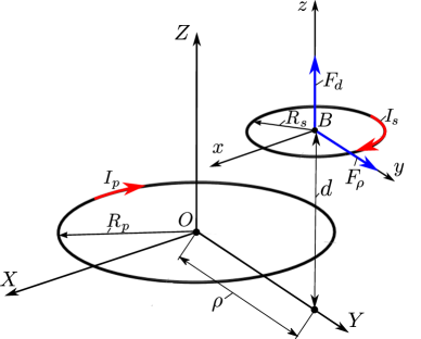
Figure 3: Geometrical scheme of circular filaments with parallel axes denoted via Grover’s notation: $\rho$ is the distance between axes; $d$ is the distance between the coils’ planes $d=z_{B}$.

4.1 Force and torque between circular filaments with parallel axes

The scheme for calculation of force and torque between circular filaments with parallel axes is shown in Fig. 3. The linear misalignment in the Grover notation can be defined by the geometrical parameter, $d$, which is the distance between the planes of circles and the parameter, $\rho$, is the distance between their axes. These parameters have the following relationship to the notation defined in this article, namely, $z_{B}=d$ and $\rho=\sqrt{x_{B}^{2}+y_{B}^{2}}$. Fig. 3 shows the particular case, when $\rho=y_{B}$, which is convenient for calculation of the restoring magnetic force $F_{y}=F_{\rho}$ and the propulsive magnetic force $F_{z}=F_{d}$ corresponding to Example 6 in Babič et al. work [38]. Also, the torque $T_{\theta}$ and $T_{\eta}$, which are directed along the $x$- and $z$-axis, respectively, is calculated.

Example 1: Force (Example 6, page 74 in Babič et al. work [38])

In this example, the restoring force (in Babič’s notation, it is denoted as $F_{r}$) between the primary filament having a radius of $R_{p}=$$42.5\text{\,}\mathrm{mm}$ and the secondary one having a radius of $R_{s}=$$20.0\text{\,}\mathrm{mm}$ was calculated. The distance between the coils’ centres is $\rho=y_{B}=$$3.0\text{\,}\mathrm{mm}$, while the distance, $d=z_{B}$, between the coils’ planes is in a range between 0 and $11\text{\,}\mathrm{mm}$. For the calculation both the developed new formula (32) and the one derived by Grover’s method (61) were used. The results of calculation are summed up in Table 1. As it can be seen from the analysis of Table 1 that all results of calculation of restoring force obtained by both formulas (32) and (61) are in an excellent agreement with results of calculation performed by Babič’s formula.

Table 1: Calculation of the restoring force for Example 1

	Babič’s	Grover’s method,	This work,
$z_{B}=d$	formula, [38, Eq. (10)],	Eq. (61),	Eq. (32),
$\mathrm{mm}$	$F_{r}=F_{\rho}$, $\mathrm{\SIUnitSymbolMicro N}$	$F_{\rho}=F_{y}$, $\mathrm{\SIUnitSymbolMicro N}$	$F_{y}=F_{\rho}$, $\mathrm{\SIUnitSymbolMicro N}$
0	0.0754774971002899	0.0754774971002898	0.0754774971002900
1.0	0.0748858332720979	0.0748858332720979	0.0748858332720979
2.0	0.0731367134919867	0.0731367134919868	0.0731367134919868
3.0	0.0703054618194718	0.0703054618194719	0.0703054618194720
4.0	0.0665103249889932	0.0665103249889937	0.0665103249889934
5.0	0.0619026566955100	0.0619026566955099	0.0619026566955097
6.0	0.0566551686796067	0.0566551686796067	0.0566551686796069
7.0	0.0509497255158943	0.0509497255158945	0.0509497255158945
8.0	0.0449660177790821	0.0449660177790823	0.0449660177790822
9.0	0.0388721123989230	0.0388721123989233	0.0388721123989234
10.0	0.0328174528506593	0.0328174528506596	0.0328174528506595
11.0	0.0269284649078899	0.0269284649078902	0.0269284649078900

Example 2: Force (Example 6, page 74 in Babič et al. work [38])

The propulsive force (in Babič’s notation, it is denoted as $F_{z}$) between the primary and second filament under the same configuration given in Example 1 was calculated. The results of calculation are shown in Table 2. Analysis of Table 2 depicts that all results of calculation obtained by new formula (33) and formula (62) derived by Grover’s method have very good agreement with results of calculation performed by Babič’s formula.

Table 2: Calculation of the propulsive force for Example 2

	Babič’s	Grover’s method,	This work,
$z_{B}=d$	formula, [38, Eq. (10)],	Eq. (62),	Eq. (33),
$\mathrm{mm}$	$F_{z}=F_{d}$, $\mathrm{\SIUnitSymbolMicro N}$	$F_{d}=F_{z}$, $\mathrm{\SIUnitSymbolMicro N}$	$F_{z}=F_{d}$, $\mathrm{\SIUnitSymbolMicro N}$
0	0.0	0.0	0.0
1.0	-0.0510570118824195	-0.0510570118824194	-0.0510570118824195
2.0	-0.101293579295215	-0.101293579295215	-0.101293579295215
3.0	-0.149926462414138	-0.149926462414137	-0.149926462414138
4.0	-0.196243385024538	-0.196243385024538	-0.196243385024538
5.0	-0.239630444882395	-0.239630444882394	-0.239630444882394
6.0	-0.279591228665736	-0.279591228665736	-0.279591228665736
7.0	-0.315756838476827	-0.315756838476827	-0.315756838476827
8.0	-0.347887153545896	-0.347887153545896	-0.347887153545896
9.0	-0.375864540746323	-0.375864540746323	-0.375864540746323
10.0	-0.399681785157597	-0.399681785157597	-0.399681785157597
11.0	-0.419426221842137	-0.419426221842137	-0.419426221842137

Table 3: Calculation of the torque $T_{\theta}$ for Example 3

$z_{B}=d$	Grover’s method,	This work,
$\mathrm{mm}$	Eq. (59), $T_{\theta}$, $\mathrm{nN}\text{\,}\mathrm{m}$	Eq. (34), $T_{\theta}$, $\mathrm{nN}\text{\,}\mathrm{m}$
0	0	0
1.0	-0.1578740617610107	-0.1578740617610108
2.0	-0.3116544572018358	-0.3116544572018354
3.0	-0.4575094468248243	-0.4575094468248247
4.0	-0.5921003456361885	-0.5921003456361873
5.0	-0.7127567873444469	-0.7127567873444469
6.0	-0.8175809895015301	-0.8175809895015308
7.0	-0.9054774849564481	-0.905477484956448
8.0	-0.9761154129579873	-0.9761154129579885
9.0	-1.029838133074231	-1.029838133074231
10.0	-1.067538737088322	-1.067538737088322
11.0	-1.090520164249831	-1.090520164249831

Table 4: Calculation of the torque $T_{\eta}$ for Example 3

$z_{B}=d$	Grover’s method,	This work,
$\mathrm{mm}$	Eq. (59), $T_{\psi}$, $\mathrm{nN}\text{\,}\mathrm{m}$	Eq. (34), $T_{\eta}$, $\mathrm{nN}\text{\,}\mathrm{m}$
0	$-1.36317281085437\times 10^{-16}$	0
1.0	$-2.000664966411278\times 10^{-16}$	0
2.0	$-1.781112775806449\times 10^{-16}$	0
3.0	$-1.996595700073574\times 10^{-16}$	0
4.0	$-1.194158312920886\times 10^{-16}$	0
5.0	$-6.21450714145062\times 10^{-17}$	0
6.0	$-9.46986487725448\times 10^{-17}$	0
7.0	$1.10795621370042\times 10^{-16}$	0
8.0	$1.548091424456673\times 10^{-16}$	0
9.0	$-2.570095735195105\times 10^{-16}$	0
10.0	$8.214737035699823\times 10^{-17}$	0
11.0	$2.123122223811704\times 10^{-16}$	0

Example 3: Torque

Considering the scheme shown in Fig. 3, the torques corresponding the generalized coordinates $\theta$ and $\eta$, namely, $T_{\theta}$ and $T_{\eta}$, respectively, are calculated by using formula (34). The calculation was performed for the same coil arrangement as in Example 1. Changing the distance, $d=z_{B}$, between the coils’ planes in the same range between 0 and $11\text{\,}\mathrm{mm}$, the obtained results of calculation of the torque $T_{\theta}$ are depicted in Table 3. While the results of calculation of the torque $T_{\eta}$ are shown in Table 4. The analysis of the tables show that the results of calculation are in excellent agreement to each other. Also, worth noting that calculation of the torque $T_{\eta}$ by means of Kalantarov-Zeitlin’s method provides the zero result for all considered cases, while the Grover method shows small errors.

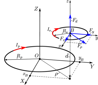
Figure 4: Geometrical scheme of circular filaments with parallel axes corresponding to the general case, when neither the $Y$-axis nor $X$-axis coincides with the $\rho$ -axis.

Example 4: Force (Example 6, page 74 in Babič et al. work [38])

Now, considering the coils having the same radii as in Example 1 and 2, but let us assume that the centre of secondary coil has the following coordinates: $x_{B}=y_{B}=~{}$$2.1213\text{\,}\mathrm{mm}$ and $z_{B}=~{}$$8.0\text{\,}\mathrm{mm}$. It means that neither the $Y$-axis nor $X$-axis coincides with the $\rho$ -axis. In this particular case, the values of coordinates $x_{B}$ and $y_{B}$ are corresponding to the Grover parameter $\rho=\sqrt{x_{B}^{2}+y_{B}^{2}}=~{}$$3.0\text{\,}\mathrm{mm}$, which has the same value as in the previous examples 1 and 2 (please see Figure 4). The restoring force with its $x$- and $y$-components and propulsive force between the primary and second filament were calculated. The results are shown in Table 5 and 6, respectively.

Table 5: Calculation of the restoring force for Example 4

This work,	$F_{x}$, $\mathrm{\SIUnitSymbolMicro N}$	$F_{y}$, $\mathrm{\SIUnitSymbolMicro N}$	$\sqrt{F_{x}^{2}+F_{y}^{2}}$, $\mathrm{\SIUnitSymbolMicro N}$
Eq. (32)	$0.031795776094544$	$0.031795776094544$	$0.0449660177790823$
Babič’s formula [38, Eq. (10)], $F_{r}$, $\mathrm{\SIUnitSymbolMicro N}$			$0.0449660177790821$
Grover’s method, Eq. (61), $F_{\rho}$, $\mathrm{\SIUnitSymbolMicro N}$			$0.0449660177790823$

Table 6: Calculation of the propulsive force for Example 4

Babič’s formula, [38, Eq. (10)],	Grover’s method,	This work,
$F_{z}$, $\mathrm{\SIUnitSymbolMicro N}$	Eq. (62), $F_{d}$, $\mathrm{\SIUnitSymbolMicro N}$	Eq. (33), $F_{z}$, $\mathrm{\SIUnitSymbolMicro N}$
$-0.347887153545896$	$-0.347887153545896$	$-0.347887153545896$

Example 5: Force (Example 8, page 75 in Babič et al. work [38])

The primary coil has a radius of $1\text{\,}\mathrm{m}$, while the secondary of $0.5\text{\,}\mathrm{m}$. The centre of the secondary coil with respect to the primary one is located at point $B$ having the following coordinate $x_{B}=y_{B}=z_{B}=~{}$$2.0\text{\,}\mathrm{m}$. The results of calculation are as follows

This work	$F_{x}$, Eq. (32) , $\mathrm{nN}$	$F_{y}$, Eq. (32), $\mathrm{nN}$	$F_{z}$, Eq. (33), $\mathrm{nN}$
	$-2.745371984357345$	$-2.745371984357349$	$3.509473102444028$
Babič’s	$F_{x}$, $\mathrm{nN}$	$F_{y}$, $\mathrm{nN}$	$F_{z}$, $\mathrm{nN}$
formula	$-2.745371984357346$	$-2.745371984357346$	$3.509473102444032$
Grover’s	–	$F_{\rho}$, Eq. (61), $\mathrm{nN}$	$F_{d}$, Eq. (62), $\mathrm{nN}$
method	–	$-3.882542294037291$	$3.50947310244403$
This work,	$\sqrt{F_{x}^{2}+F_{y}^{2}}$, $\mathrm{nN}$:	$3.882542294037292$	–

Example 6: Force, the special case of $\theta=\pi/2$ (Example 9, page 76 in Babič et al. work [38])

The primary coil has a radius of $1\text{\,}\mathrm{m}$, while the secondary of $0.5\text{\,}\mathrm{m}$. The centre of the secondary coil with respect to the primary one is located at point $B$ having the following coordinate $x_{B}=$$1.0\text{\,}\mathrm{m}$, $y_{B}=$$2.0\text{\,}\mathrm{m}$, $z_{B}=~{}$$3.0\text{\,}\mathrm{m}$. The secondary coil is located on the plane $x=$ $1.0\text{\,}\mathrm{m}$ ($\theta=\eta=$$\pi\text{/}2\text{\,}\mathrm{rad}$). For the calculation, Eq. (43) and (44) are used. Results are

This work	$F_{x}$, Eq. (43) , $\mathrm{nN}$	$F_{y}$, Eq. (43), $\mathrm{nN}$	$F_{z}$, Eq. (44), $\mathrm{nN}$
	$1.939241379554505$	$-1.861181718234279$	$-2.202382194552672$
Babič’s	$F_{x}$, $\mathrm{nN}$	$F_{y}$, $\mathrm{nN}$	$F_{z}$, $\mathrm{nN}$
formula	$1.939241379554508$	$-1.861181718234281$	$-2.202382194552672$

Example 7: Torque (the singular case of Kalantarov-Zeitlin’s method)

For the same arrangement of coils as in Example 6 above, the torque $T_{\eta}$ is calculated by formula (45). This case corresponds to the singularity of Kalantarov-Zeitlin’s method for the calculation of the torque $T_{\theta}$. Due to this fact the value is not available in the table below. The results are

This work,	$T_{\theta}$, $\mathrm{nN}\text{\,}\mathrm{m}$	$T_{\eta}$, $\mathrm{nN}\text{\,}\mathrm{m}$
Eq. (45):	$--$	$6.860953527497655$
Grover’s method,	$T_{\theta}$, $\mathrm{nN}\text{\,}\mathrm{m}$	$T_{\psi}$, $\mathrm{nN}\text{\,}\mathrm{m}$
Eq. (63):	$-6.036471731788468$	$6.860953527497664$

However, to avoid this difficulty the angle $\theta$ can be chosen enough close to the value $\pi/2$, but not equal to it. Hence, formula (34) can be applied. For instance, if the angle $\theta$ is $1.570\,62\text{\,}\mathrm{rad}$, the result of calculation of the torque $T_{\theta}$ becomes $-6.036\,471\,614\,863\,915\text{\,}\mathrm{nN}\text{\,}\mathrm{m}$ with a relative error of $-1.93696844616845\times 10^{-8}$ in comparing with the exact result of calculation obtained by means of Grover’s method.

Example 8: Force, the special case of $\theta=\pi/2$ (Example 10, page 76 in Babič et al. work [38])

The primary and secondary coils have the same radii as in example 5. While, the centre of the secondary coil with respect to the primary one is located at point $B$ having the coordinate: $x_{B}=y_{B}=z_{B}=$$2.0\text{\,}\mathrm{m}$. The secondary coil is located on the plane $y=$ $2.0\text{\,}\mathrm{m}$ ($\theta=$ $\pi\text{/}2\text{\,}\mathrm{rad}$ and $\eta=$$0\text{\,}\mathrm{rad}$). For the calculation, as in the previous example Eq. (43) and (44) are used. The results are

This work	$F_{x}$, Eq. (43), $\mathrm{nN}$	$F_{y}$, Eq. (43), $\mathrm{nN}$	$F_{z}$, Eq. (44), $\mathrm{nN}$
	$4.901398177052338$	$1.984872313200136$	$2.582265710169335$
The Babič	$F_{x}$, $\mathrm{nN}$	$F_{y}$, $\mathrm{nN}$	$F_{z}$, $\mathrm{nN}$
formula	$4.901398177052345$	$1.984872313200137$	$2.582265710169336$

Example 9: Force

The primary and secondary coils have the same radii as in example 5 (the primary coil has a radius of $1\text{\,}\mathrm{m}$ and the secondary one of $0.5\text{\,}\mathrm{m}$). The centre of the secondary coil with respect to the primary one is located at point $B$ having the coordinates: $x_{B}=0$ and $y_{B}=z_{B}=$$2.0\text{\,}\mathrm{m}$ ($\theta=0$ and $\eta=$$0\text{\,}\mathrm{rad}$). The results of calculation are as follows

This work:
$F_{x}$, Eq. (32), $\mathrm{nN}$	$F_{y}$, Eq. (32), $\mathrm{nN}$	$F_{z}$, Eq. (33), $\mathrm{nN}$
$-2.943923360032078\times 10^{-15}$	$-13.05164071847218$	$0.5836068102838426$
The Grover method:	$F_{\rho}$, Eq. (61), $\mathrm{nN}$	$F_{d}$, Eq. (62), $\mathrm{nN}$
–	$-13.05164071847219$	$0.583606810283838$

Example 10: Force, the special case of $\theta=\pi/2$

The primary and secondary coils have the same radii as in example 5 (the primary coil has a radius of $1\text{\,}\mathrm{m}$ and the secondary one of $0.5\text{\,}\mathrm{m}$). The centre of the secondary coil with respect to the primary one is located at point $B$ having the coordinates: $x_{B}=0$ and $y_{B}=z_{B}=$$2.0\text{\,}\mathrm{m}$. While, the angular orientation of the secondary coil is defined as follows $\theta=\pi/2$ and $\eta=$$0\text{\,}\mathrm{rad}$. The results of calculation are

This work:
$F_{x}$, Eq. (43), $\mathrm{nN}$	$F_{y}$, Eq. (43), $\mathrm{nN}$	$F_{z}$, Eq. (44) , $\mathrm{nN}$
$-3.986562883376773\times 10^{-16}$	$9.62480501067982$	$12.81718822413886$
The Grover method:	$F_{\rho}$, Eq. (61), $\mathrm{nN}$	$F_{d}$, Eq. (62), $\mathrm{nN}$
–	$9.624805010679824$	$12.81718822413886$

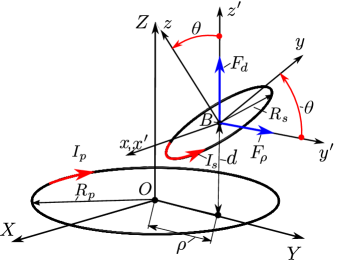
Figure 5: Geometrical scheme of circular filaments with intersect axes.

4.2 Force and torque between inclined circular filaments with intersect axes

The general scheme of the arrangement of two inclined circular filaments whose axes intersect for calculation of the force and torque is shown in Fig. 5. The centre $B$ of the secondary circle is located on the $ZY$- plane and the $xy$ plane of the secondary circle is inclined by the $\theta$ angle ($\eta=0$).

Example 11: Force

The primary and secondary coils have the same radii as in examples 7 and 8 (the primary coil has a radius of $1\text{\,}\mathrm{m}$ and the secondary one of $0.5\text{\,}\mathrm{m}$). Also, similar to Example 7 and 8, the centre of the secondary coil with respect to the primary one is located at point $B$ having the coordinates: $x_{B}=0$ and $y_{B}=z_{B}=$$2.0\text{\,}\mathrm{m}$, while the angel of $\theta$ is changed in a range from $\pi/12$ to $5\pi\text{/}12\text{\,}\mathrm{rad}$. Hence, the results of calculation of force are as follows.

For the angle of $\theta=$$\pi\text{/}12\text{\,}\mathrm{rad}$, results are

This work:
$F_{x}$, Eq. (32), $\mathrm{nN}$	$F_{y}$, Eq. (32), $\mathrm{nN}$	$F_{z}$, Eq. (33) , $\mathrm{nN}$
$-3.925231146709438\times 10^{-15}$	$-10.83934689818066$	$4.085335195849623$
The Grover method:	$F_{\rho}$, Eq. (61), $\mathrm{nN}$	$F_{d}$, Eq. (62), $\mathrm{nN}$
–	$-10.83934689818066$	$4.08533519584963$

For the angle of $\theta=$$\pi\text{/}6\text{\,}\mathrm{rad}$, results are

This work:
$F_{x}$, Eq. (32), $\mathrm{nN}$	$F_{y}$, Eq. (32), $\mathrm{nN}$	$F_{z}$, Eq. (33) , $\mathrm{nN}$
$-2.943923360032078\times 10^{-15}$	$-7.552692503639927$	$7.633101747693313$
The Grover method:	$F_{\rho}$, Eq. (61), $\mathrm{nN}$	$F_{d}$, Eq. (62), $\mathrm{nN}$
–	$-7.552692503639934$	$7.633101747693303$

For the angle of $\theta=$$\pi\text{/}4\text{\,}\mathrm{rad}$, results are

This work:
$F_{x}$, Eq. (32), $\mathrm{nN}$	$F_{y}$, Eq. (32), $\mathrm{nN}$	$F_{z}$, Eq. (33) , $\mathrm{nN}$
$-2.943923360032078\times 10^{-15}$	$-3.307376210012321$	$10.68822709927552$
The Grover method:	$F_{\rho}$, Eq. (61), $\mathrm{nN}$	$F_{d}$, Eq. (62), $\mathrm{nN}$
–	$-3.307376210012323$	$10.6882270992755$

For the angle of $\theta=$$\pi\text{/}3\text{\,}\mathrm{rad}$, results are

This work:
$F_{x}$, Eq. (32), $\mathrm{nN}$	$F_{y}$, Eq. (32), $\mathrm{nN}$	$F_{z}$, Eq. (33) , $\mathrm{nN}$
$-9.813077866773594\times 10^{-16}$	$1.423367390491171$	$12.68704579579398$
The Grover method:	$F_{\rho}$, Eq. (61), $\mathrm{nN}$	$F_{d}$, Eq. (62), $\mathrm{nN}$
–	$1.42336739049117$	$12.68704579579398$

For the angle of $\theta=$$5\pi\text{/}12\text{\,}\mathrm{rad}$, results are

This work:
$F_{x}$, Eq. (32), $\mathrm{nN}$	$F_{y}$, Eq. (32), $\mathrm{nN}$	$F_{z}$, Eq. (33) , $\mathrm{nN}$
$4.906538933386797\times 10^{-16}$	$5.934542693142568$	$13.34958760362382$
The Grover method:	$F_{\rho}$, Eq. (61), $\mathrm{nN}$	$F_{d}$, Eq. (62), $\mathrm{nN}$
–	$5.934542693142566$	$13.3495876036238$

Example 12: Torque

Now, for the same coil arrangement as in Example 10 above, the components of the torque were calculated. The results are as follows.

For the angle of $\theta=$$\pi\text{/}12\text{\,}\mathrm{rad}$, results are

This work,	$T_{\theta}$, $\mathrm{nN}\text{\,}\mathrm{m}$	$T_{\eta}$, $\mathrm{nN}\text{\,}\mathrm{m}$
Eq. (34):	$-16.91560720972092$	$-1.103971260012029\times 10^{-15}$
The Grover method,	$T_{\theta}$, $\mathrm{nN}\text{\,}\mathrm{m}$	$T_{\psi}$, $\mathrm{nN}\text{\,}\mathrm{m}$
Eq. (59):	$-16.91560720972094$	$3.496810701779198\times 10^{-15}$

For the angle of $\theta=$$\pi\text{/}6\text{\,}\mathrm{rad}$, results are

This work,	$T_{\theta}$, $\mathrm{nN}\text{\,}\mathrm{m}$	$T_{\eta}$, $\mathrm{nN}\text{\,}\mathrm{m}$
Eq. (34):	$-18.05278139644676$	$-1.717288626685379\times 10^{-15}$
The Grover method,	$T_{\theta}$, $\mathrm{nN}\text{\,}\mathrm{m}$	$T_{\psi}$, $\mathrm{nN}\text{\,}\mathrm{m}$
Eq. (59):	$-18.05278139644677$	$2.99873918328272\times 10^{-16}$

For the angle of $\theta=$$\pi\text{/}4\text{\,}\mathrm{rad}$, results are

This work,	$T_{\theta}$, $\mathrm{nN}\text{\,}\mathrm{m}$	$T_{\eta}$, $\mathrm{nN}\text{\,}\mathrm{m}$
Eq. (34):	$-17.23198131459169$	$4.599880250050123\times 10^{-15}$
The Grover method,	$T_{\theta}$, $\mathrm{nN}\text{\,}\mathrm{m}$	$T_{\psi}$, $\mathrm{nN}\text{\,}\mathrm{m}$
Eq. (59):	$-17.23198131459168$	$-2.386186316760677\times 10^{-16}$

For the angle of $\theta=$$\pi\text{/}3\text{\,}\mathrm{rad}$, results are

This work,	$T_{\theta}$, $\mathrm{nN}\text{\,}\mathrm{m}$	$T_{\eta}$, $\mathrm{nN}\text{\,}\mathrm{m}$
Eq. (34):	$-14.34174801596063$	$3.925231146709438\times 10^{-15}$
The Grover method,	$T_{\theta}$, $\mathrm{nN}\text{\,}\mathrm{m}$	$T_{\psi}$, $\mathrm{nN}\text{\,}\mathrm{m}$
Eq. (59):	$-14.34174801596063$	$-1.034553191651082\times 10^{-15}$

For the angle of $\theta=$$5\pi\text{/}12\text{\,}\mathrm{rad}$, results are

This work,	$T_{\theta}$, $\mathrm{nN}\text{\,}\mathrm{m}$	$T_{\eta}$, $\mathrm{nN}\text{\,}\mathrm{m}$
Eq. (34):	$-10.05276095457351$	$1.177569344012831\times 10^{-14}$
The Grover method,	$T_{\theta}$, $\mathrm{nN}\text{\,}\mathrm{m}$	$T_{\psi}$, $\mathrm{nN}\text{\,}\mathrm{m}$
Eq. (59):	$-10.05276095457353$	$2.72021517637498\times 10^{-16}$

4.3 Force and torque between circular filaments arbitrarily positioned in the space

The validation of the developed formulas, namely, for force calculation (32), (33) and for torque calculation (34) between circular filaments arbitrarily positioned in the space as shown in Fig. 6 is performed by comparison with the results of calculation obtained by utilizing Grover’s method. The position of the secondary coil with respect to the primary one is determined by the linear and angular misalignment, in particular, the angular one is defined by the $\eta$- and $\theta$-angle.

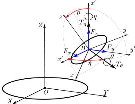
Figure 6: Geometrical scheme for calculation of force and torque between circular filaments arbitrarily positioned in the space: the angular misalignment is determined by the $\eta$- and $\theta$-angle.

Example 13: Force

The primary and secondary circles have radii $R_{p}=$$16.0\text{\,}\mathrm{cm}$ and $R_{s}=$$10.0\text{\,}\mathrm{cm}$, respectively. The centre of the secondary circle is located at $x_{B}=0$, $y_{B}=$$4.3301\text{\,}\mathrm{cm}$, $z_{B}=$$17.5\text{\,}\mathrm{cm}$ and the angle, $\theta$ of $60.0\text{\,}\mathrm{\SIUnitSymbolDegree}$, but the angle $\eta$ is varied in a range from 0 to 360$\mathrm{\SIUnitSymbolDegree}$. The arrangement corresponds to one considered in Babič et al. work [39] for calculation of mutual inductance. The results of calculation are summed up below.

For the angle of $\eta=$$0\text{\,}\mathrm{rad}$, results are

This work:
$F_{x}$, Eq. (32), $\mathrm{\SIUnitSymbolMicro N}$	$F_{y}$, Eq. (32), $\mathrm{\SIUnitSymbolMicro N}$	$F_{z}$, Eq. (33) , $\mathrm{nN}$
$-9.12816701829942\times 10^{-17}$	$-0.178854052497651$	$-0.120726650359416$
The Grover method:	$F_{\rho}$, Eq. (61), $\mathrm{\SIUnitSymbolMicro N}$	$F_{d}$, Eq. (62), $\mathrm{\SIUnitSymbolMicro N}$
–	$-0.178854052497651$	$-0.120726650359416$

For the angle of $\eta=$$\pi\text{/}6\text{\,}\mathrm{rad}$, results are

This work:
$F_{x}$, Eq. (32), $\mathrm{\SIUnitSymbolMicro N}$	$F_{y}$, Eq. (32), $\mathrm{\SIUnitSymbolMicro N}$	$F_{z}$, Eq. (33) , $\mathrm{nN}$
$0.0739614721316561$	$-0.159981513393707$	$-0.128840188997851$
The Grover method:	$F_{\rho}$, Eq. (61), $\mathrm{\SIUnitSymbolMicro N}$	$F_{d}$, Eq. (62), $\mathrm{\SIUnitSymbolMicro N}$
–	$-0.159981513393707$	$-0.128840188997851$

For the angle of $\eta=$$\pi\text{/}3\text{\,}\mathrm{rad}$, results are

This work:
$F_{x}$, Eq. (32), $\mathrm{\SIUnitSymbolMicro N}$	$F_{y}$, Eq. (32), $\mathrm{\SIUnitSymbolMicro N}$	$F_{z}$, Eq. (33) , $\mathrm{nN}$
$0.128768354487727$	$-0.108439678353152$	$-0.151814417341889$
The Grover method:	$F_{\rho}$, Eq. (61), $\mathrm{\SIUnitSymbolMicro N}$	$F_{d}$, Eq. (62), $\mathrm{\SIUnitSymbolMicro N}$
–	$-0.108439678353152$	$-0.151814417341889$

For the angle of $\eta=$$\pi\text{/}2\text{\,}\mathrm{rad}$, results are

This work:
$F_{x}$, Eq. (32), $\mathrm{\SIUnitSymbolMicro N}$	$F_{y}$, Eq. (32), $\mathrm{\SIUnitSymbolMicro N}$	$F_{z}$, Eq. (33) , $\mathrm{nN}$
$0.150180118721259$	$-0.0376756210066879$	$-0.18544258034698$
The Grover method:	$F_{\rho}$, Eq. (61), $\mathrm{\SIUnitSymbolMicro N}$	$F_{d}$, Eq. (62), $\mathrm{\SIUnitSymbolMicro N}$
–	$-0.037675621006688$	$-0.18544258034698$

For the angle of $\eta=$$2\pi\text{/}3\text{\,}\mathrm{rad}$, results are

This work:
$F_{x}$, Eq. (32), $\mathrm{\SIUnitSymbolMicro N}$	$F_{y}$, Eq. (32), $\mathrm{\SIUnitSymbolMicro N}$	$F_{z}$, Eq. (33) , $\mathrm{nN}$
$0.13174801806108$	$0.034039013278426$	$-0.222277730943632$
The Grover method:	$F_{\rho}$, Eq. (61), $\mathrm{\SIUnitSymbolMicro N}$	$F_{d}$, Eq. (62), $\mathrm{\SIUnitSymbolMicro N}$
–	$0.034039013278426$	$-0.222277730943632$

For the angle of $\eta=$$5\pi\text{/}6\text{\,}\mathrm{rad}$, results are

This work:
$F_{x}$, Eq. (32), $\mathrm{\SIUnitSymbolMicro N}$	$F_{y}$, Eq. (32), $\mathrm{\SIUnitSymbolMicro N}$	$F_{z}$, Eq. (33) , $\mathrm{nN}$
$0.0768930004431087$	$0.0873707070288501$	$-0.251739105122414$
The Grover method:	$F_{\rho}$, Eq. (61), $\mathrm{\SIUnitSymbolMicro N}$	$F_{d}$, Eq. (62), $\mathrm{\SIUnitSymbolMicro N}$
–	$0.0873707070288498$	$-0.251739105122414$

For the angle of $\eta=$$\pi\text{\,}\mathrm{rad}$, results are

This work:
$F_{x}$, Eq. (32), $\mathrm{\SIUnitSymbolMicro N}$	$F_{y}$, Eq. (32), $\mathrm{\SIUnitSymbolMicro N}$	$F_{z}$, Eq. (33) , $\mathrm{nN}$
$-2.38736675863216\times 10^{-16}$	$0.107078490953807$	$-0.263132411165356$
The Grover method:	$F_{\rho}$, Eq. (61), $\mathrm{\SIUnitSymbolMicro N}$	$F_{d}$, Eq. (62), $\mathrm{\SIUnitSymbolMicro N}$
–	$0.107078490953807$	$-0.263132411165356$

For the angle of $\eta=$$7\pi\text{/}6\text{\,}\mathrm{rad}$, results are

This work:
$F_{x}$, Eq. (32), $\mathrm{\SIUnitSymbolMicro N}$	$F_{y}$, Eq. (32), $\mathrm{\SIUnitSymbolMicro N}$	$F_{z}$, Eq. (33) , $\mathrm{nN}$
$-0.0768930004431088$	$0.08737070702885$	$-0.251739105122414$
The Grover method:	$F_{\rho}$, Eq. (61), $\mathrm{\SIUnitSymbolMicro N}$	$F_{d}$, Eq. (62), $\mathrm{\SIUnitSymbolMicro N}$
–	$0.0873707070288499$	$-0.251739105122414$

For the angle of $\eta=$$4\pi\text{/}3\text{\,}\mathrm{rad}$, results are

This work:
$F_{x}$, Eq. (32), $\mathrm{\SIUnitSymbolMicro N}$	$F_{y}$, Eq. (32), $\mathrm{\SIUnitSymbolMicro N}$	$F_{z}$, Eq. (33) , $\mathrm{nN}$
$-0.13174801806108$	$0.0340390132784261$	$-0.222277730943632$
The Grover method:	$F_{\rho}$, Eq. (61), $\mathrm{\SIUnitSymbolMicro N}$	$F_{d}$, Eq. (62), $\mathrm{\SIUnitSymbolMicro N}$
–	$0.0340390132784261$	$-0.222277730943632$

For the angle of $\eta=$$3\pi\text{/}2\text{\,}\mathrm{rad}$, results are

This work:
$F_{x}$, Eq. (32), $\mathrm{\SIUnitSymbolMicro N}$	$F_{y}$, Eq. (32), $\mathrm{\SIUnitSymbolMicro N}$	$F_{z}$, Eq. (33) , $\mathrm{nN}$
$-0.150180118721259$	$-0.0376756210066879$	$-0.18544258034698$
The Grover method:	$F_{\rho}$, Eq. (61), $\mathrm{\SIUnitSymbolMicro N}$	$F_{d}$, Eq. (62), $\mathrm{\SIUnitSymbolMicro N}$
–	$-0.0376756210066879$	$-0.18544258034698$

For the angle of $\eta=$$5\pi\text{/}3\text{\,}\mathrm{rad}$, results are

This work:
$F_{x}$, Eq. (32), $\mathrm{\SIUnitSymbolMicro N}$	$F_{y}$, Eq. (32), $\mathrm{\SIUnitSymbolMicro N}$	$F_{z}$, Eq. (33) , $\mathrm{nN}$
$-0.128768354487727$	$-0.108439678353152$	$-0.151814417341889$
The Grover method:	$F_{\rho}$, Eq. (61), $\mathrm{\SIUnitSymbolMicro N}$	$F_{d}$, Eq. (62), $\mathrm{\SIUnitSymbolMicro N}$
–	$-0.108439678353152$	$-0.151814417341889$

For the angle of $\eta=$$11\pi\text{/}6\text{\,}\mathrm{rad}$, results are

This work:
$F_{x}$, Eq. (32), $\mathrm{\SIUnitSymbolMicro N}$	$F_{y}$, Eq. (32), $\mathrm{\SIUnitSymbolMicro N}$	$F_{z}$, Eq. (33) , $\mathrm{nN}$
$-0.0739614721316564$	$-0.159981513393707$	$-0.128840188997851$
The Grover method:	$F_{\rho}$, Eq. (61), $\mathrm{\SIUnitSymbolMicro N}$	$F_{d}$, Eq. (62), $\mathrm{\SIUnitSymbolMicro N}$
–	$-0.159981513393707$	$-0.128840188997851$

For the angle of $\eta=$$2\pi\text{\,}\mathrm{rad}$, results are

This work:
$F_{x}$, Eq. (32), $\mathrm{\SIUnitSymbolMicro N}$	$F_{y}$, Eq. (32), $\mathrm{\SIUnitSymbolMicro N}$	$F_{z}$, Eq. (33) , $\mathrm{nN}$
$-2.24693341988909\times 10^{-16}$	$-0.178854052497651$	$-0.120726650359416$
The Grover method:	$F_{\rho}$, Eq. (61), $\mathrm{\SIUnitSymbolMicro N}$	$F_{d}$, Eq. (62), $\mathrm{\SIUnitSymbolMicro N}$
–	$-0.178854052497651$	$-0.120726650359416$

Example 14: Torque

For the same arrangement of coils as in Example 13 above, the torque is calculated. Results are shown below.

For the angle of $\theta=$$0\text{\,}\mathrm{rad}$, results are

This work,	$T_{\theta}$, $\mathrm{nN}\text{\,}\mathrm{m}$	$T_{\eta}$, $\mathrm{nN}\text{\,}\mathrm{m}$
Eq. (34):	$-35.67279850151469$	$-2.10650008114602\times 10^{-15}$
The Grover method,	$T_{\theta}$, $\mathrm{nN}\text{\,}\mathrm{m}$	$T_{\psi}$, $\mathrm{nN}\text{\,}\mathrm{m}$
Eq. (59):	$-35.67279850151468$	$7.820828205289753\times 10^{-16}$

For the angle of $\eta=$$\pi\text{/}6\text{\,}\mathrm{rad}$, results are

This work,	$T_{\theta}$, $\mathrm{nN}\text{\,}\mathrm{m}$	$T_{\eta}$, $\mathrm{nN}\text{\,}\mathrm{m}$
Eq. (34):	$-34.95015525890449$	$3.202605704772845$
The Grover method,	$T_{\theta}$, $\mathrm{nN}\text{\,}\mathrm{m}$	$T_{\psi}$, $\mathrm{nN}\text{\,}\mathrm{m}$
Eq. (59):	$-34.95015525890452$	$3.202605704772839$

For the angle of $\eta=$$\pi\text{/}3\text{\,}\mathrm{rad}$, results are

This work,	$T_{\theta}$, $\mathrm{nN}\text{\,}\mathrm{m}$	$T_{\eta}$, $\mathrm{nN}\text{\,}\mathrm{m}$
Eq. (34):	$-32.95959317516494$	$5.575798517673081$
The Grover method,	$T_{\theta}$, $\mathrm{nN}\text{\,}\mathrm{m}$	$T_{\psi}$, $\mathrm{nN}\text{\,}\mathrm{m}$
Eq. (59):	$-32.95959317516493$	$5.575798517673075$

For the angle of $\eta=$$\pi\text{/}2\text{\,}\mathrm{rad}$, results are

This work,	$T_{\theta}$, $\mathrm{nN}\text{\,}\mathrm{m}$	$T_{\eta}$, $\mathrm{nN}\text{\,}\mathrm{m}$
Eq. (34):	$-30.16106072467219$	$6.502949320749249$
The Grover method,	$T_{\theta}$, $\mathrm{nN}\text{\,}\mathrm{m}$	$T_{\psi}$, $\mathrm{nN}\text{\,}\mathrm{m}$
Eq. (59):	$-30.16106072467218$	$6.502949320749247$

For the angle of $\eta=$$2\pi\text{/}3\text{\,}\mathrm{rad}$, results are

This work,	$T_{\theta}$, $\mathrm{nN}\text{\,}\mathrm{m}$	$T_{\eta}$, $\mathrm{nN}\text{\,}\mathrm{m}$
Eq. (34):	$-27.19599671483476$	$5.704820930062833$
The Grover method,	$T_{\theta}$, $\mathrm{nN}\text{\,}\mathrm{m}$	$T_{\psi}$, $\mathrm{nN}\text{\,}\mathrm{m}$
Eq. (59):	$-27.19599671483475$	$5.704820930062828$

For the angle of $\eta=$$5\pi\text{/}6\text{\,}\mathrm{rad}$, results are

This work,	$T_{\theta}$, $\mathrm{nN}\text{\,}\mathrm{m}$	$T_{\eta}$, $\mathrm{nN}\text{\,}\mathrm{m}$
Eq. (34):	$-24.8616946084914$	$3.329543812187064$
The Grover method,	$T_{\theta}$, $\mathrm{nN}\text{\,}\mathrm{m}$	$T_{\psi}$, $\mathrm{nN}\text{\,}\mathrm{m}$
Eq. (59):	$-24.86169460849138$	$3.329543812187052$

For the angle of $\eta=$$\pi\text{\,}\mathrm{rad}$, results are

This work,	$T_{\theta}$, $\mathrm{nN}\text{\,}\mathrm{m}$	$T_{\eta}$, $\mathrm{nN}\text{\,}\mathrm{m}$
Eq. (34):	$-23.96174184275239$	$5.617333549722721\times 10^{-15}$
The Grover method,	$T_{\theta}$, $\mathrm{nN}\text{\,}\mathrm{m}$	$T_{\psi}$, $\mathrm{nN}\text{\,}\mathrm{m}$
Eq. (59):	$-23.96174184275239$	$4.791446029057778\times 10^{-15}$

For the angle of $\eta=$$7\pi\text{/}6\text{\,}\mathrm{rad}$, results are

This work,	$T_{\theta}$, $\mathrm{nN}\text{\,}\mathrm{m}$	$T_{\eta}$, $\mathrm{nN}\text{\,}\mathrm{m}$
Eq. (34):	$-24.8616946084914$	$-3.329543812187048$
The Grover method,	$T_{\theta}$, $\mathrm{nN}\text{\,}\mathrm{m}$	$T_{\psi}$, $\mathrm{nN}\text{\,}\mathrm{m}$
Eq. (59):	$-24.86169460849138$	$-3.329543812187046$

For the angle of $\eta=$$4\pi\text{/}3\text{\,}\mathrm{rad}$, results are

This work,	$T_{\theta}$, $\mathrm{nN}\text{\,}\mathrm{m}$	$T_{\eta}$, $\mathrm{nN}\text{\,}\mathrm{m}$
Eq. (34):	$-27.19599671483477$	$-5.704820930062826$
The Grover method,	$T_{\theta}$, $\mathrm{nN}\text{\,}\mathrm{m}$	$T_{\psi}$, $\mathrm{nN}\text{\,}\mathrm{m}$
Eq. (59):	$-27.19599671483473$	$-5.704820930062823$

For the angle of $\eta=$$3\pi\text{/}2\text{\,}\mathrm{rad}$, results are

This work,	$T_{\theta}$, $\mathrm{nN}\text{\,}\mathrm{m}$	$T_{\eta}$, $\mathrm{nN}\text{\,}\mathrm{m}$
Eq. (34):	$-30.16106072467218$	$-6.502949320749249$
The Grover method,	$T_{\theta}$, $\mathrm{nN}\text{\,}\mathrm{m}$	$T_{\psi}$, $\mathrm{nN}\text{\,}\mathrm{m}$
Eq. (59):	$-30.16106072467218$	$-6.502949320749249$

For the angle of $\eta=$$5\pi\text{/}3\text{\,}\mathrm{rad}$, results are

This work,	$T_{\theta}$, $\mathrm{nN}\text{\,}\mathrm{m}$	$T_{\eta}$, $\mathrm{nN}\text{\,}\mathrm{m}$
Eq. (34):	$-32.95959317516493$	$-5.575798517673075$
The Grover method,	$T_{\theta}$, $\mathrm{nN}\text{\,}\mathrm{m}$	$T_{\psi}$, $\mathrm{nN}\text{\,}\mathrm{m}$
Eq. (59):	$-32.95959317516497$	$-5.575798517673072$

For the angle of $\eta=$$11\pi\text{/}6\text{\,}\mathrm{rad}$, results are

This work,	$T_{\theta}$, $\mathrm{nN}\text{\,}\mathrm{m}$	$T_{\eta}$, $\mathrm{nN}\text{\,}\mathrm{m}$
Eq. (34):	$-34.95015525890449$	$-3.202605704772844$
The Grover method,	$T_{\theta}$, $\mathrm{nN}\text{\,}\mathrm{m}$	$T_{\psi}$, $\mathrm{nN}\text{\,}\mathrm{m}$
Eq. (59):	$-34.95015525890452$	$-3.202605704772843$

For the angle of $\eta=$$2\pi\text{\,}\mathrm{rad}$, results are

This work,	$T_{\theta}$, $\mathrm{nN}\text{\,}\mathrm{m}$	$T_{\eta}$, $\mathrm{nN}\text{\,}\mathrm{m}$
Eq. (34):	$-35.6727985015147$	$-1.40433338743068\times 10^{-15}$
The Grover method,	$T_{\theta}$, $\mathrm{nN}\text{\,}\mathrm{m}$	$T_{\psi}$, $\mathrm{nN}\text{\,}\mathrm{m}$
Eq. (59):	$-35.6727985015147$	$3.112983652841607\times 10^{-16}$

5 Conclusion

We derived new formulas, namely, (32), (33), (34), (43), (44) and (45) for calculation of force and torque between two circular filaments arbitrarily oriented in space presented in the integral analytical form, whose kernel function is expressed in terms of the elliptic integrals of the first and second kinds. In particular, formulas (43), (44) and (45) are applied for the special case ($\theta=$$\pi\text{/}2\text{\,}\mathrm{rad}$), when the circular filaments are mutually perpendicular to each other. For calculation of the torque $T_{\theta}$, this special case corresponds to the singularity one. To avoid this difficulty, it is suggested that the angle $\theta$ can be chosen enough close to the value $\pi/2$, but not equal to it and calculation is performed by means of formula (34). Thus, the developed formulas are applicable for all possible arrangements between two circular filaments.

New developed formulas have been successfully validated through a number of examples available in the literature and direct comparison with results of calculation of force and torque performed by expressions derived by Grover’s method. Besides, the obtained formulas can be easily programmed, they are intuitively understandable for application.

Appendix A Calculation of force and torque between two arbitrarily oriented circular filaments using Grover’s formula of mutual inductance [42, page 207, Eq. (179)]

Figure 7: Geometrical scheme of arbitrarily oriented circular filaments: the Grover notations.

According to Grover’s notations, the linear misalignment of the centre of the secondary circle is characterised by two parameters, namely, $d=z_{B}$ and $\rho=\sqrt{x_{B}^{2}+y_{B}^{2}}$ as shown in Figure 7. Besides that the angular misalignment is defined in accordance with the first manner as shown in Fig. 2, but keeping the original Grover’s notation the angle, $\eta$, is replaced by $\psi$. In absence of the angular misalignment, the CF $xyz$ assigned to the secondary circle is oriented in the following way. The $z$-axis is directed upward along the $d$-line, while the $y$-axis is parallel to the $\rho$-line and directed in continuation of the $\rho$-line. Then adopting the above considered notations, Grover’s formula for calculation of mutual inductance between two circular filaments can be written as

$$M=\frac{\mu_{0}\sqrt{R_{p}R_{s}}}{2\pi}\int_{0}^{2\pi}U\cdot\Psi(k)d\varphi,$$ (46)

where

$$U=U({\gamma},\theta,\psi)=\frac{R({\gamma},\theta,\psi)}{{V}^{1.5}}=\frac{\cos\theta-\gamma(\cos\psi\cos\varphi-\sin\psi\cos\theta\sin\varphi)}{{V}^{1.5}},$$ (47)

$$V=V({\gamma},\theta,\psi)=\sqrt{1-{\cos(\varphi)}^{2}{\sin(\theta)}^{2}+2\gamma(\sin\psi\sin\varphi-\cos\varphi\cos\psi\cos\theta)+\gamma^{2}},$$ (48)

$$\Psi(k)=\frac{2}{k}\left[\left(1-\frac{k^{2}}{2}\right)K(k)-E(k)\right],$$ (49)

$$\begin{array}[]{l}{\displaystyle k^{2}=k^{2}({\gamma},\Delta,\theta,\psi)=\frac{4\alpha{V}}{(\alpha{V}+1)^{2}+z^{2}},}\\ {\displaystyle\alpha=R_{s}/R_{p},\;\Delta=d/R_{p},\;\gamma=\rho/R_{s}},\;z={\Delta}-{\alpha}\sin\theta\cos\varphi.\end{array}$$ (50)

The kernel of formula (46) is

$$\mathrm{Kr}=U\cdot\Psi(k).$$ (51)

Accounting for (47), (48), (49) and (50), the $\rho$-derivative of the kernel becomes

$${\displaystyle\frac{\partial\mathrm{Kr}}{\partial\rho}=\frac{\partial\mathrm{Kr}}{\partial\gamma}\frac{1}{R_{s}}=\frac{1}{R_{s}}\cdot\left[\frac{\partial U}{\partial\gamma}\cdot\Psi(k)+U\cdot\frac{d\Psi(k)}{dk}\cdot\frac{\partial k}{\partial\gamma}\right],}$$ (52)

where

$$\begin{array}[]{l}{\displaystyle\frac{\partial U}{\partial\gamma}=\left({\displaystyle\frac{\partial R}{\partial\gamma}}\cdot V-1.5\cdot R\cdot\frac{\partial V}{\partial\gamma}\right)\bigg{/}{{V}^{2.5}},}\\ {\displaystyle\frac{\partial R}{\partial\gamma}=-(\cos\psi\cos\varphi-\sin\psi\cos\theta\sin\varphi),}\\ {\displaystyle\frac{\partial V}{\partial\gamma}=\frac{\sin\psi\,\sin\varphi-\cos\varphi\,\cos\psi\,\cos\theta+\gamma}{V},}\\ {\displaystyle\frac{\partial k}{\partial\gamma}=\frac{2/k-k(\alpha{V}+1)}{(\alpha{V}+1)^{2}+{z}^{2}}\cdot\alpha\frac{\partial V}{\partial\gamma},}\end{array}$$ (53)

$$\frac{d\Psi(k)}{dk}=\frac{2}{k^{2}}\left[\frac{2-k^{2}}{2(1-k^{2})}E(k)-K(k)\right].$$ (54)

The $d$-derivative of the kernel is

$${\displaystyle\frac{\partial\mathrm{Kr}}{\partial d}=\frac{\partial\mathrm{Kr}}{\partial\Delta}\frac{1}{R_{p}}=\frac{1}{R_{p}}\cdot U\cdot\frac{d\Psi(k)}{dk}\cdot\frac{\partial k}{\partial\Delta},}$$ (55)

where

$$\begin{array}[]{l}{\displaystyle\frac{\partial k}{\partial\Delta}=-\frac{k\cdot z}{(\alpha{V}+1)^{2}+{z}^{2}}\cdot\frac{\partial z}{\partial\Delta},}\\ {\displaystyle\frac{\partial z}{\partial\Delta}=1.}\end{array}$$ (56)

Note that in Eq. (55) the $k$-derivative of $\Psi(k)$ is defined similarly as in Eq. (54). The derivatives of the kernel with respect to the angular coordinates are as follows. The $\theta$-derivative is

$${\displaystyle\frac{\partial\mathrm{Kr}}{\partial\theta}=\frac{\partial U}{\partial\theta}\cdot\Psi(k)+U\cdot\frac{d\Psi(k)}{dk}\cdot\frac{\partial k}{\partial\theta},}$$ (57)

where

$$\begin{array}[]{l}{\displaystyle\frac{\partial U}{\partial\theta}=\left({\displaystyle\frac{\partial R}{\partial\theta}}\cdot V-1.5\cdot R\cdot\frac{\partial V}{\partial\theta}\right)\bigg{/}{{V}^{2.5}},}\\ {\displaystyle\frac{\partial R}{\partial\theta}=-\sin\theta\cdot(1+\gamma\cdot\sin\varphi\,\sin\psi),}\\ {\displaystyle\frac{\partial V}{\partial\theta}=\frac{-\sin\theta\cdot({\cos(\varphi)}^{2}\,\cos\theta-\gamma\cdot\cos\varphi\,\cos\psi)}{V},}\\ {\displaystyle\frac{\partial k}{\partial\theta}=\frac{\left[2/k-k(\alpha{V}+1)\right]{\displaystyle\cdot\alpha\frac{\partial V}{\partial\theta}}-k\cdot z\cdot{\displaystyle\frac{\partial z}{\partial\theta}}}{(\alpha{V}+1)^{2}+{z}^{2}},}\\ {\displaystyle\frac{\partial z}{\partial\theta}=-\alpha\cdot\cos\theta\cos\varphi.}\end{array}$$ (58)

The $\psi$-derivative is

$${\displaystyle\frac{\partial\mathrm{Kr}}{\partial\psi}=\frac{\partial U}{\partial\psi}\cdot\Psi(k)+U\cdot\frac{d\Psi(k)}{dk}\cdot\frac{\partial k}{\partial\psi},}$$ (59)

where

$$\begin{array}[]{l}{\displaystyle\frac{\partial U}{\partial\psi}=\left({\displaystyle\frac{\partial R}{\partial\psi}}\cdot V-1.5\cdot R\cdot\frac{\partial V}{\partial\psi}\right)\bigg{/}{{V}^{2.5}},}\\ {\displaystyle\frac{\partial R}{\partial\psi}=\gamma\cdot(\cos\varphi\,\sin\psi+\sin\varphi\,\cos\psi\,\cos\theta),}\\ {\displaystyle\frac{\partial V}{\partial\psi}=\frac{\gamma\cdot(\sin\varphi\,\cos\psi+\cos\varphi\,\sin\psi\,\cos\theta)}{V},}\\ {\displaystyle\frac{\partial k}{\partial\psi}=\frac{2/k-k(\alpha{V}+1)}{(\alpha{V}+1)^{2}+{z}^{2}}\cdot{\displaystyle\alpha\frac{\partial V}{\partial\psi}},}\\ {\displaystyle\frac{\partial z}{\partial\psi}=0.}\end{array}$$ (60)

Using the derivatives of the kernel obtained above, we can write the first derivatives of Grover’s formula of mutual inductance with respect to the appropriate coordinates. Taking into account Eq. (52), the $\rho$-derivative of Grover’s formula (46) is

$$\frac{\partial\mathrm{M}}{\partial\rho}=\frac{\mu_{0}}{2\pi}\sqrt{\frac{R_{p}}{R_{s}}}\int_{0}^{2\pi}\frac{\partial U}{\partial\gamma}\cdot\Psi(k)+U\cdot\frac{d\Psi(k)}{dk}\cdot\frac{\partial k}{\partial\gamma}\;\;d\varphi.$$ (61)

Accounting for (55), the $d$-derivative of Grover’s formula (46) can be written as

$$\frac{\partial\mathrm{M}}{\partial d}=\frac{\mu_{0}}{2\pi}\sqrt{\frac{R_{s}}{R_{p}}}\int_{0}^{2\pi}U\cdot\frac{d\Psi(k)}{dk}\cdot\frac{\partial k}{\partial\Delta}\;\;d\varphi.$$ (62)

Considering Eq. (57) and (59), first derivatives of Grover’s formula (46) of with respect to angular coordinates can be written

$$\frac{\partial\mathrm{M}}{\partial g}=\frac{\mu_{0}\sqrt{R_{p}R_{s}}}{2\pi}\int_{0}^{2\pi}\frac{\partial U}{\partial g}\cdot\Psi(k)+U\cdot\frac{d\Psi(k)}{dk}\cdot\frac{\partial k}{\partial g}\;\;d\varphi,$$ (63)

where $g=\theta$ and $\psi$, respectively.

The derived formulas (61), (62) and (63) can be easily programmed by using, for instance, Matlab language. The file with Matlab code with implemented formulas is available for a reader in supplementary materials to this article.

References

- [1] E. Okress, D. Wroughton, G. Comenetz, P. Brace, J. Kelly, Electromagnetic levitation of solid and molten metals, Journal of Applied Physics 23 (5) (1952) 545–552.
-
[2]
Y. M. Urman, Theory for the
calculation of the force characteristics of an electromagnetic suspension of
a superconducting body, Technical Physics 42 (1) (1997) 1–6.
doi:10.1134/1.1258645.
URL https://doi.org/10.1134/1.1258645 -
[3]
Y. M. Urman, Calculation of the force
characteristics of a multi-coil suspension of a superconducting sphere,
Technical Physics 42 (1) (1997) 7–13.
doi:10.1134/1.1258654.
URL https://doi.org/10.1134/1.1258654 - [4] M. W. Coffey, Mutual inductance of superconducting thin films, Journal of Applied Physics 89 (10) (2001) 5570–5577.
- [5] Y. Urman, S. Kuznetsov, Translational transformations of tensor solutions of the helmholtz equation and their application to describe interactions in force fields of various physical nature, Quarterly of Applied Mathematics 72 (1) (2014) 1–20.
- [6] U.-M. Jow, M. Ghovanloo, Design and optimization of printed spiral coils for efficient transcutaneous inductive power transmission, IEEE Transactions on biomedical circuits and systems 1 (3) (2007) 193–202.
- [7] Y. P. Su, X. Liu, S. Y. R. Hui, Mutual inductance calculation of movable planar coils on parallel surfaces, IEEE Transactions on Power Electronics 24 (4) (2009) 1115–1123. doi:10.1109/TPEL.2008.2009757.
- [8] S. Y. Chu, A. T. Avestruz, Transfer-power measurement: A non-contact method for fair and accurate metering of wireless power transfer in electric vehicles, in: 2017 IEEE 18th Workshop on Control and Modeling for Power Electronics (COMPEL), 2017, pp. 1–8. doi:10.1109/COMPEL.2017.8013344.
- [9] A. Shiri, A. Shoulaie, A new methodology for magnetic force calculations between planar spiral coils, Progress In Electromagnetics Research 95 (2009) 39–57.
- [10] R. Ravaud, G. Lemarquand, V. Lemarquand, Force and stiffness of passive magnetic bearings using permanent magnets. part 1: Axial magnetization, IEEE transactions on magnetics 45 (7) (2009) 2996.
- [11] S. Obata, A muscle motion solenoid actuator, Electrical Engineering in Japan 184 (2) (2013) 10–19.
-
[12]
R. Shalati, K. V. Poletkin, J. G. Korvink, V. Badilita,
Novel concept of a
series linear electromagnetic array artificial muscle, Journal of Physics:
Conference Series 1052 (1) (2018) 012047.
URL http://stacks.iop.org/1742-6596/1052/i=1/a=012047 -
[13]
K. Poletkin, A. I. Chernomorsky, C. Shearwood, U. Wallrabe,
An analytical model of
micromachined electromagnetic inductive contactless suspension., in: the
ASME 2013 International Mechanical Engineering Congress & Exposition, ASME,
San Diego, California, USA, 2013, pp. V010T11A072–V010T11A072.
doi:10.1115/IMECE2013-66010.
URL http://dx.doi.org/10.1115/IMECE2013-66010 -
[14]
K. Poletkin, A. Chernomorsky, C. Shearwood, U. Wallrabe,
A qualitative
analysis of designs of micromachined electromagnetic inductive contactless
suspension, International Journal of Mechanical Sciences 82 (2014) 110–121.
doi:10.1016/j.ijmecsci.2014.03.013.
URL http://authors.elsevier.com/sd/article/S0020740314000897 -
[15]
Z. Lu, K. Poletkin, B. den Hartogh, U. Wallrabe, V. Badilita,
3D micro-machined
inductive contactless suspension: Testing and modeling, Sensors and
Actuators A Physical 220 (2014) 134–143.
doi:10.1016/j.sna.2014.09.017.
URL http://dx.doi.org/10.1016/j.sna.2014.09.017 -
[16]
K. Poletkin, Z. Lu, U. Wallrabe, J. Korvink, V. Badilita,
Stable
dynamics of micro-machined inductive contactless suspensions, International
Journal of Mechanical Sciences 131-132 (2017) 753 – 766.
doi:https://doi.org/10.1016/j.ijmecsci.2017.08.016.
URL http://www.sciencedirect.com/science/article/pii/S0020740316306555 -
[17]
V. Vlnieska, A. Voigt, S. Wadhwa, J. Korvink, M. Kohl, K. Poletkin,
Development of control circuit
for inductive levitation micro-actuators, Proceedings 64 (1).
doi:10.3390/IeCAT2020-08479.
URL https://www.mdpi.com/2504-3900/64/1/39 - [18] K. V. Poletkin, A. I. Chernomorsky, C. Shearwood, A proposal for micromachined accelerometer, base on a contactless suspension with zero spring constant, IEEE Sensors J. 12 (07) (2012) 2407–2413. doi:10.1109/JSEN.2012.2188831.
-
[19]
K. V. Poletkin, R. Shalati, J. G. Korvink, V. Badilita,
Pull-in actuation in
hybrid micro-machined contactless suspension, Journal of Physics: Conference
Series 1052 (1) (2018) 012035.
URL http://stacks.iop.org/1742-6596/1052/i=1/a=012035 - [20] K. V. Poletkin, J. G. Korvink, Modeling a pull-in instability in micro-machined hybrid contactless suspension 7 (1) (2018) 11.
-
[21]
K. Poletkin, Static pull-in
behavior of hybrid levitation micro-actuators: simulation, modelling and
experimental study, IEEE/ASME Transactions on Mechatronicsdoi:10.1109/TMECH.2020.2999516.
URL https://doi.org/10.1109/TMECH.2020.2999516 - [22] T. Theodoulidis, R. J. Ditchburn, Mutual impedance of cylindrical coils at an arbitrary position and orientation above a planar conductor, IEEE Transactions on Magnetics 43 (8) (2007) 3368–3370. doi:10.1109/TMAG.2007.894559.
-
[23]
M. Sawan, S. Hashemi, M. Sehil, F. Awwad, M. Hajj-Hassan, A. Khouas,
Multicoils-based inductive
links dedicated to power up implantable medical devices: modeling, design and
experimental results, Biomedical Microdevices 11 (5) (2009) 1059.
doi:10.1007/s10544-009-9323-7.
URL https://doi.org/10.1007/s10544-009-9323-7 -
[24]
S. Kuznetsov, J. K. Guest,
Topology
optimization of magnetic source distributions for diamagnetic and
superconducting levitation, Journal of Magnetism and Magnetic Materials 438
(2017) 60 – 69.
doi:https://doi.org/10.1016/j.jmmm.2017.04.052.
URL http://www.sciencedirect.com/science/article/pii/S0304885316319515 -
[25]
D. Hoult, B. Tomanek,
Use of
mutually inductive coupling in probe design, Concepts in Magnetic Resonance
15 (4) (2002) 262–285.
arXiv:https://onlinelibrary.wiley.com/doi/pdf/10.1002/cmr.10047,
doi:10.1002/cmr.10047.
URL https://onlinelibrary.wiley.com/doi/abs/10.1002/cmr.10047 -
[26]
N. Spengler, P. T. While, M. V. Meissner, U. Wallrabe, J. G. Korvink,
Magnetic lenz lenses
improve the limit-of-detection in nuclear magnetic resonance, PLOS ONE
12 (8) (2017) 1–17.
doi:10.1371/journal.pone.0182779.
URL https://doi.org/10.1371/journal.pone.0182779 - [27] G. D. Angelis, V. Pasku, A. D. Angelis, M. Dionigi, M. Mongiardo, A. Moschitta, P. Carbone, An indoor ac magnetic positioning system, IEEE Transactions on Instrumentation and Measurement 64 (5) (2015) 1267–1275. doi:10.1109/TIM.2014.2381353.
- [28] F. Wu, J. Jeon, S. K. Moon, H. J. Choi, H. Son, Voice coil navigation sensor for flexible silicone intubation, IEEE/ASME Transactions on Mechatronics 21 (2) (2016) 851–859. doi:10.1109/TMECH.2015.2476836.
- [29] X. Zhang, C. Quan, Z. Li, Mutual inductance calculation of circular coils for an arbitrary position with electromagnetic shielding in wireless power transfer systems, IEEE Transactions on Transportation Electrification (2021) 1–1doi:10.1109/TTE.2021.3054762.
- [30] B. Gulbahar, A communication theoretical analysis of multiple-access channel capacity in magneto-inductive wireless networks, IEEE Transactions on Communications 65 (6) (2017) 2594–2607. doi:10.1109/TCOMM.2017.2669995.
- [31] J. C. Maxwell, A Treatise on Electricity and Magnetism, 3rd Edition, Vol. 2, Dover Publications Inc., 1954.
- [32] C. Snow, Formulas for computing capacitance and inductance, Vol. 544, US Govt. Print. Off., 1954.
- [33] K.-B. Kim, E. Levi, Z. Zabar, L. Birenbaum, Restoring force between two noncoaxial circular coils, IEEE Transactions on Magnetics 32 (2) (1996) 478–484.
- [34] F. W. Grover, The calculation of the mutual inductance of circular filaments in any desired positions, Proceedings of the IRE 32 (10) (1944) 620–629. doi:10.1109/JRPROC.1944.233364.
-
[35]
S. I. Babic, C. Akyel, Y. Ren, W. Chen,
Magnetic force calculation
between circular coils of rectangular cross section with parallel axes for
superconducting magnet, Progress In Electromagnetics Research 37 (2012)
275–288.
doi:10.2528/PIERB11110508.
URL http://dx.doi.org/10.2528/PIERB11110508 - [36] S. I. Babic, C. Akyel, Torque calculation between circular coils with inclined axes in air, International Journal of Numerical Modelling: Electronic Networks, Devices and Fields 24 (3) (2011) 230–243.
- [37] S. I. Babic, C. Akyel, New formulas for calculating torque between filamentary circular coil and thin wall solenoid with inclined axis whose axes are at the same plane, Progress In Electromagnetics Research 73 (2018) 141–151.
- [38] S. Babic, C. Akyel, Magnetic force between inclined circular filaments placed in any desired position, IEEE transactions on magnetics 48 (1) (2012) 69–80.
-
[39]
S. Babic, F. Sirois, C. Akyel, C. Girardi,
Mutual inductance
calculation between circular filaments arbitrarily positioned in space:
Alternative to Grover’s formula, IEEE Transactions on Magnetics 46 (9)
(2010) 3591–3600.
doi:10.1109/TMAG.2010.2047651.
URL https://doi.org/10.1109/TMAG.2010.2047651 - [40] P. L. Kalantarov, L. A. Zeitlin, Raschet induktivnostey (Calculation of Inductances), 3rd Edition, Energoatomizdat, Leningrad, 1986.
-
[41]
K. V. Poletkin, J. G. Korvink,
Efficient
calculation of the mutual inductance of arbitrarily oriented circular
filaments via a generalisation of the Kalantarov-Zeitlin method, Journal
of Magnetism and Magnetic Materials 483 (2019) 10–20.
doi:https://doi.org/10.1016/j.jmmm.2019.03.078.
URL https://www.sciencedirect.com/science/article/pii/S0304885318337703 - [42] F. W. Grover, Inductance calculations : working formulas and tables, special ed. prepared for instrument society of america Edition, Research Triangle Park, N.C. : Instrument Society of America, 1981, reprint. Originally published: New York : Van Nostrand, 1946. With publisher’s comment.