Investigations of the linear and non-linear flow harmonics
using the A Multi-Phase Transport model
Abstract
The Multi-Phase Transport model (AMPT) is used to study the effects of the parton-scattering cross-sections () and hadronic re-scattering on the linear contributions to the flow harmonic , the non-linear response coefficients, and the correlations between different order flow symmetry planes in Au+Au collisions at 200 GeV. The model results, which agree with current experimental measurements, indicate that the higher-order flow harmonics are sensitive to the variations. However, the non-linear response coefficients and the correlations between different order flow symmetry planes are independent. These results suggest that further detailed experimental measurements which span a broad range of collision systems and beam energies could serve as an additional constraint for the theoretical models’ calculations.
I Introduction
Numerous experimental investigations of heavy-ion collisions at the Large Hadron Collider (LHC) and the Relativistic Heavy Ion Collider (RHIC) indicate the creation of the matter predicted by Quantum Chromodynamics (QCD), called Quark-Gluon Plasma (QGP) Shuryak (1978, 1980); Muller et al. (2012), in these collisions. Many of the previous and current experimental investigations in heavy-ion collisions are aimed at a better understanding of the QGP transport properties (especially, ) Shuryak (2004); Romatschke and Romatschke (2007); Luzum and Romatschke (2008); Bozek (2010); Acharya et al. (2019, 2020a); Adam et al. (2020).
A wealth of knowledge about was obtained by studying the anisotropic flow observables. The anisotropic flow measurements are expected to display the viscous hydrodynamic response to the initial spatial distribution formed in the collision’s early stages Heinz and Kolb (2002); Hirano et al. (2006); Huovinen et al. (2001); Hirano and Tsuda (2002); Romatschke and Romatschke (2007); Luzum (2011); Song et al. (2011); Qian et al. (2016); Magdy (2018, 2017); Schenke et al. (2011); Teaney and Yan (2012); Gardim et al. (2012a); Lacey et al. (2016). Anisotropic flow can be represented via the Fourier expansion Poskanzer and Voloshin (1998) of the distribution of the particle azimuthal angle , as;
| (1) |
where represents the value of the order flow harmonic, and is the reaction plane defined by the beam direction and impact parameter Poskanzer and Voloshin (1998). The is called directed flow, is named elliptic flow, and is termed triangular flow, etc. The earlier investigations of flow correlations and fluctuations Adam et al. (2018, 2016); Adamczyk et al. (2018a); Qiu and Heinz (2011); Adare et al. (2011); Aad et al. (2014, 2015a); Magdy (2019a); Alver et al. (2008, 2010a); Ollitrault et al. (2009) and higher-order flow coefficients Magdy (2019b); Adam et al. (2019); Magdy (2019a); Adamczyk et al. (2018b); Magdy (2017); Adamczyk et al. (2018a); Alver and Roland (2010); Chatrchyan et al. (2014), have guided us toward a better understanding of the QGP properties.
In a hydrodynamic-like scenario, anisotropic flow is driven by the spatial anisotropy of the initial-state energy density, characterized by the complex eccentricity vector Alver et al. (2010b); Petersen et al. (2010); Lacey et al. (2011); Teaney and Yan (2011); Qiu and Heinz (2011):
where and are the value and azimuthal direction of the n eccentricity vector, , , is the spatial azimuthal angle, and is the initial anisotropic energy density profile Teaney and Yan (2011); Bhalerao et al. (2015); Yan and Ollitrault (2015). To a good degree the Adamczyk et al. (2016a, b); Magdy (2019a); Adamczyk et al. (2015); Wei et al. (2018) and Adamczyk et al. (2016c); Adam et al. (2019) are linearly related to and , respectively Song et al. (2011); Niemi et al. (2013); Gardim et al. (2015); Fu (2015); Holopainen et al. (2011); Qin et al. (2010); Qiu and Heinz (2011); Gale et al. (2013); Liu and Lacey (2018):
| (3) |
where is expected to be sensitive to the QGP Adam et al. (2019); Heinz and Snellings (2013). Although the lower- and higher-order flow harmonics are emerging from linear response to the same-order eccentricity, the higher-order harmonics, , in addition, contains a non-linear response to the lower-order eccentricities Teaney and Yan (2012); Bhalerao et al. (2015); Yan and Ollitrault (2015); Gardim et al. (2012b):
| (4) | |||||
where carry information about the medium properties as well as the coupling between the lower and higher order eccentricity harmonicsLiu and Lacey (2018). The terms and are the linear and the non-linear contributions respectively. The represents the non-linear response coefficients.
The non-linear contribution to will display the correlation between different order flow symmetry planes. This correlation is expected to shed light on the heavy-ion collisions’ initial stage dynamics Bilandzic et al. (2014); Bhalerao et al. (2015); Aad et al. (2015a); Adam et al. (2016, 2018); Zhou (2016); Qiu and Heinz (2012); Teaney and Yan (2014); Niemi et al. (2016); Zhou et al. (2016); Zhao et al. (2017). The linear and non-linear contributions to higher-order flow harmonics have been discussed in several experimental publications Magdy (2021); Sirunyan et al. (2020); Acharya et al. (2020b, c, 2021); Adam et al. (2020); Aad et al. (2015b). In addition, they are also widely discussed in several phenomenological studies using different transport and hydrodynamic models Magdy et al. (2020); Yang et al. (2020); Liu and Lacey (2018); Bozek (2018); Chattopadhyay et al. (2018); Zhao et al. (2017).
In this work, I investigated the influence of the parton-scattering cross-sections () and the hadronic re-scattering on the linear and non-linear contributions to the as well as the coupling constant () and the correlations between different order flow symmetry planes (). Here, an important objective is to gain improved insights on the sensitivity of these measures to the initial-state geometry and the medium’s properties. Note that in transport models Lin et al. (2005) have been related to the final state transport confection Xu and Ko (2011a); Nasim (2017); Solanki et al. (2013). The current sensitivity study, conducted within the AMPT model Lin et al. (2005) framework, could lend important insights on ongoing beam energy measurements Magdy (2021) of the linear and non-linear contributions to designed to constrain the dependence of on and .
II Methodology
II.1 The AMPT model
This investigation is conducted with simulated events for Au–Au collisions at = 200 GeV, obtained using the AMPT Lin et al. (2005) model. Calculations were made for charged hadrons in the transverse momentum span GeV/ and the pseudorapidity acceptance . The latter selection mimics the acceptance of the STAR experiment at RHIC.
The AMPT model Lin et al. (2005) is widely employed to investigate the physics of the relativistic heavy-ion collisions at LHC and RHIC energies Lin et al. (2005); Ma and Lin (2016); Haque et al. (2019); Bhaduri and Chattopadhyay (2010); Nasim et al. (2010); Xu and Ko (2011b); Magdy et al. (2020); Guo et al. (2019). In this study, simulations were performed with the string melting option in the AMPT model both on and off. In a string melting scenario hadrons produced using the HIJING model are converted to their valence quarks and anti-quarks, and their evolution in time and space is then evaluated by the ZPC parton cascade model Zhang (1998). The essential components of AMPT are (i) an HIJING model Wang and Gyulassy (1991); Gyulassy and Wang (1994) initial parton-production stage, (ii) a parton-scattering stage, (iii) hadronization through coalescence followed by (iv) a hadronic interaction stage Li and Ko (1995). In the parton-scattering stage the employed parton-scattering cross-sections are estimated according to;
| (5) |
where is the QCD coupling constant and is the screening mass in the partonic matter. They generally give the expansion dynamics of the A–A collision systems Zhang (1998); Within the AMPT framework, the initial value of (evaluated at the beginning of heavy-ion collision) can be related to see Refs Xu and Ko (2011a); Nasim (2017); Solanki et al. (2013).
In this work, Au+Au collisions at 200 GeV, were simulated with AMPT version ampt-v2.26t9b for a fixed value of = 0.47, but varying in the range 2.26 – 4.2 Xu and Ko (2011a); Nasim (2017). The presented AMPT sets in this work are given in Tab. 1.
| AMPT-set | String Melting Mechanism | |
|---|---|---|
| Set-1 | 6.1 | OFF |
| Set-2 | 6.1 | ON |
| Set-3 | 2.7 | ON |
| Set-4 | 1.8 | ON |
The results presented in sec. II.2, were obtained for minimum bias Au–Au collisions at 200 GeV. A total of approximately 4.0, 5.0, 4.0, and 3.0 M events of Au–Au collisions were generated with AMPT Set-1, Set-2, Set-3, and Set-4, respectively.
II.2 Analysis Method
The two- and multi-particle cumulants methods Bilandzic et al. (2011, 2014); Gajdošová (2017); Jia et al. (2017), are used in this work. The two- and multi-particle cumulants can be constructed in terms of nth flow vectors () magnitude. The are given as:
| (6) |
where is the total number of particles in an event and is the particle weight. We also introduce the sum over the particles weight as:
| (7) |
Using Eqs.(6, 7) the two-, three-, and four-particle correlations were constructed using the two-subevents cumulant methods Jia et al. (2017), with ( and ).
| (8) |
| (9) |
| (10) |
The benefit of using the two-subevents technique is that it assists the reduction of the nonflow correlations due to resonance decays, Bose-Einstein correlations, and the fragments of individual jets Magdy et al. (2020).
The non-linear contribution to can be given as Yan and Ollitrault (2015); Bhalerao et al. (2013):
| (11) |
and the linear contribution to can be expressed as:
| (12) |
Equation (12) suggests that and are independent Yan and Ollitrault (2015); Magdy et al. (2020).
The non-linear response coefficient (), which quantify the mode-coupling contributions to the , is defined as:
| (13) |
The correlations between different order flow symmetry planes () Acharya et al. (2017) can be given as:
| (14) |
III Results and discussion
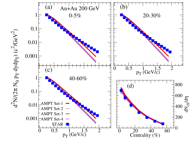
Before I present the AMPT model flow harmonics results, I first compare the AMPT model transverse momentum spectra and the charged-particle multiplicity density with the experimental measurements Adams et al. (2003); Abelev et al. (2009). Fig. 1 shows the transverse momentum spectra (a)-(c) and the charged-particle multiplicity density (d) for Au+Au collisions at 200 GeV from the AMPT model. The model results are also compared to the STAR collaboration measurements (solid points) Adams et al. (2003); Abelev et al. (2009). They indicate that the AMPT results agree with the STAR measurements at low (1.3 GeV/) but fails to explain the data for larger . By contrast, AMPT shows good overall agreement with the experimental charged-particle multiplicity density.
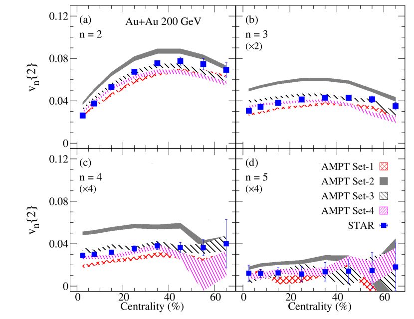
The extraction of the linear and the non-linear contributions to relies on the two- and multiparticle correlations. Therefore, it is instructive to investigate the dependence of these variables on the model parameters tabulated in Table 1. Fig. 2 shows a comparison of the centrality dependence of (a)-(d) for Au–Au collisions at 200 GeV from the AMPT model. The presented from the AMPT exhibit a sensitivity to both and whether or not string melting is turned on. They also indicate similar patterns to the data reported by the STAR collaboration Adamczyk et al. (2016c, 2018a) (solid points) depending on the model parameters given in Table 1.
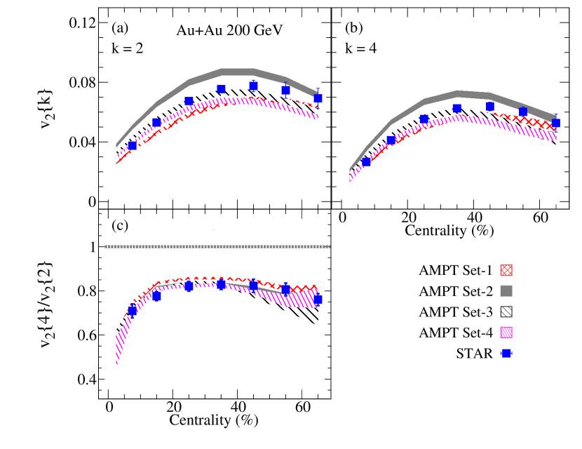
Figure 3 shows a comparison of the centrality dependence of (a), (b) and the ratios (c) for the AMPT model. The results presented in Fig. 3 panels (a) and (b) show that AMPT (k=2 and 4) are sensitive to the model parameters tabulated in Tab. 1.They also give similar values and trends to those measured by the STAR experiment Adams et al. (2005). The ratios , shown in panel (c), work as a figure of merit for the elliptic flow fluctuations strength; correspond to minimal flow fluctuations and decreasing values of for larger flow fluctuations. The estimated ratios, which are in good agreement with the experimental ratios, are to within 2% insensitive to the model setups given in Tab. 1, implying that the flow fluctuations in the AMPT model are eccentricity-driven and are roughly a constant fraction of .
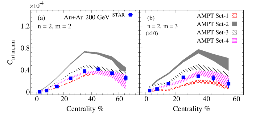
The centrality dependence of the three-particle correlators, and , are shown in Fig. 4 for Au+Au collisions at 200 GeV from the AMPT model. These results indicate that and are strongly sensitive to the and also sensitive to whether or not string melting is turned on. They also show patterns similar to the experimental data reported by the STAR collaboration Adam et al. (2020).
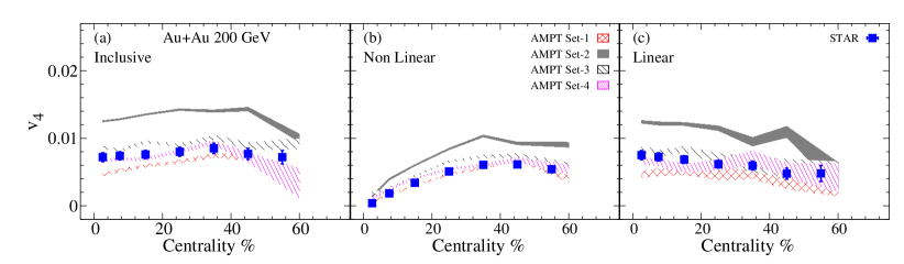
The centrality dependence of the inclusive, linear and non-linear for Au+Au collisions at = 200 GeV from the AMPT model are shown in Fig. 5. The presented measurements indicate that the linear contribution of which is the dominant contribution to the inclusive in central collisions has a weak centrality dependence. The presented results show that the inclusive, linear and non-linear are sensitive to the . These results are compared to STAR collaboration measurements Adam et al. (2020). The AMPT model simulations indicate similar qualitative patterns to the measured by the STAR collaboration Adam et al. (2020).
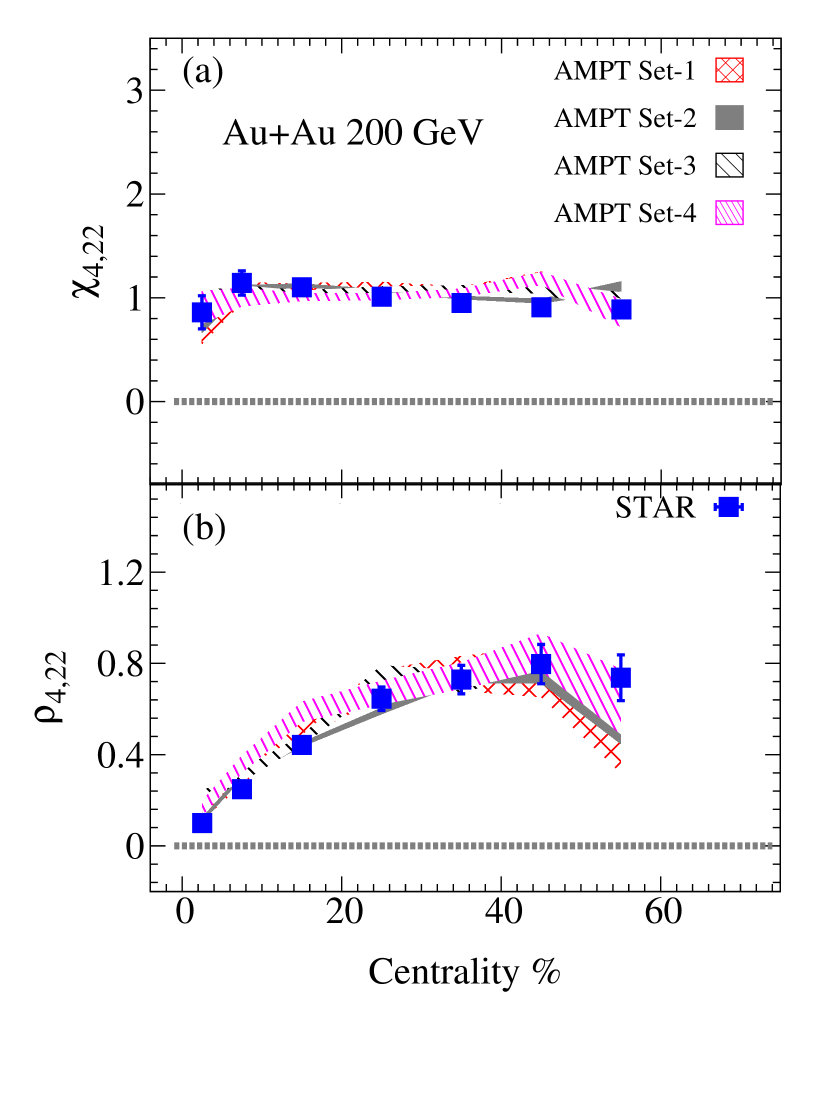
The centrality dependence of the non-linear response coefficients, , for Au+Au collisions at = 200 GeV, from the AMPT model is presented in Fig. 6(a). The results indicate a weak centrality and dependence, which implies that (i) the non-linear centrality dependence arises from the lower-order flow harmonics and (ii) the is dominated by initial-state eccentricity couplings. The from the AMPT model shows a good agreement with the measured by the STAR experiment Adam et al. (2020).
Figure 6(b) shows the centrality dependence of the correlations of the event plane angles, , in Au–Au collisions at = 200 GeV from the AMPT model. The results imply stronger event plane correlations in peripheral collisions for all presented AMPT sets. However, the calculated magnitudes of are shown and found to be independent of . Such observation suggests that the correlation of event plane angles are dominated by initial-state correlations. The from the AMPT model indicate a good agreement with the measured by the STAR collaboration Adam et al. (2020).
IV Conclusions
In summary, I have presented extensive AMPT model studies to evaluate the dependence of the linear and non-linear contributions to the , non-linear response coefficients, and the correlations of the event plane angle for Au–Au collisions at = 200 GeV. The presented AMPT calculations indicate a strong centrality dependence for the non-linear in contrast, the linear shows a soft centrality dependence. In addition, calculations show a strong sensitivity to the and whether or not string melting is turned on. The dimensionless parameters and show magnitudes and trends which are independent, suggesting that the correlations of event plane angles, as well as the non-linear response coefficients, are dominated by initial-state effects. Based on these AMPT model calculations, I conclude that conducting further detailed experimental measurements of the linear and non-linear response to the higher-order flow harmonics over a broad range of beam-energies and for different collision systems could serve as an additional constraint for theoretical models.
Acknowledgments
This research is supported by the US Department of Energy, Office of Nuclear Physics (DOE NP), under contracts DE-FG02-94ER40865.
References
- Shuryak (1978) E. V. Shuryak, Phys. Lett. B 78, 150 (1978).
- Shuryak (1980) E. V. Shuryak, Phys. Rept. 61, 71 (1980).
- Muller et al. (2012) B. Muller, J. Schukraft, and B. Wyslouch, Ann. Rev. Nucl. Part. Sci. 62, 361 (2012).
- Shuryak (2004) E. Shuryak, Prog. Part. Nucl. Phys. 53, 273 (2004).
- Romatschke and Romatschke (2007) P. Romatschke and U. Romatschke, Phys.Rev.Lett. 99, 172301 (2007).
- Luzum and Romatschke (2008) M. Luzum and P. Romatschke, Phys.Rev. C78, 034915 (2008).
- Bozek (2010) P. Bozek, Phys. Rev. C 81, 034909 (2010).
- Acharya et al. (2019) S. Acharya et al. (ALICE), Phys. Rev. Lett. 123, 142301 (2019).
- Acharya et al. (2020a) S. Acharya et al. (ALICE), JHEP 05, 085 (2020a).
- Adam et al. (2020) J. Adam et al. (STAR), Phys. Lett. B 809, 135728 (2020).
- Heinz and Kolb (2002) U. W. Heinz and P. F. Kolb, Statistical QCD. Proceedings, International Symposium, Bielefeld, Germany, August 26-30, 2001, Nucl. Phys. A702, 269 (2002).
- Hirano et al. (2006) T. Hirano, U. W. Heinz, D. Kharzeev, R. Lacey, and Y. Nara, Phys.Lett. B636, 299 (2006).
- Huovinen et al. (2001) P. Huovinen, P. F. Kolb, U. W. Heinz, P. V. Ruuskanen, and S. A. Voloshin, Phys. Lett. B503, 58 (2001).
- Hirano and Tsuda (2002) T. Hirano and K. Tsuda, Phys. Rev. C66, 054905 (2002).
- Luzum (2011) M. Luzum, J. Phys. G38, 124026 (2011).
- Song et al. (2011) H. Song, S. A. Bass, U. Heinz, T. Hirano, and C. Shen, Phys. Rev. Lett. 106, 192301 (2011), [Erratum: Phys. Rev. Lett.109,139904(2012)].
- Qian et al. (2016) J. Qian, U. W. Heinz, and J. Liu, Phys. Rev. C93, 064901 (2016).
- Magdy (2018) N. Magdy (STAR), Proceedings, 11th International Workshop on Critical Point and Onset of Deconfinement (CPOD2017): Stony Brook, NY, USA, August 7-11, 2017, PoS CPOD2017, 005 (2018).
- Magdy (2017) N. Magdy (STAR), Proceedings, 16th International Conference on Strangeness in Quark Matter (SQM 2016): Berkeley, California, United States, J. Phys. Conf. Ser. 779, 012060 (2017).
- Schenke et al. (2011) B. Schenke, S. Jeon, and C. Gale, Phys.Lett. B702, 59 (2011).
- Teaney and Yan (2012) D. Teaney and L. Yan, Phys. Rev. C86, 044908 (2012).
- Gardim et al. (2012a) F. G. Gardim, F. Grassi, M. Luzum, and J.-Y. Ollitrault, Phys.Rev.Lett. 109, 202302 (2012a).
- Lacey et al. (2016) R. A. Lacey, D. Reynolds, A. Taranenko, N. N. Ajitanand, J. M. Alexander, F.-H. Liu, Y. Gu, and A. Mwai, J. Phys. G43, 10LT01 (2016).
- Poskanzer and Voloshin (1998) A. M. Poskanzer and S. A. Voloshin, Phys. Rev. C58, 1671 (1998).
- Adam et al. (2018) J. Adam et al. (STAR), Phys. Lett. B783, 459 (2018).
- Adam et al. (2016) J. Adam et al. (ALICE), Phys. Rev. Lett. 117, 182301 (2016).
- Adamczyk et al. (2018a) L. Adamczyk et al. (STAR), Phys. Rev. C98, 034918 (2018a).
- Qiu and Heinz (2011) Z. Qiu and U. W. Heinz, Phys. Rev. C84, 024911 (2011).
- Adare et al. (2011) A. Adare et al. (PHENIX), Phys. Rev. Lett. 107, 252301 (2011).
- Aad et al. (2014) G. Aad et al. (ATLAS), Phys. Rev. C90, 024905 (2014).
- Aad et al. (2015a) G. Aad et al. (ATLAS), Phys. Rev. C92, 034903 (2015a).
- Magdy (2019a) N. Magdy (STAR), Proceedings, 27th International Conference on Ultrarelativistic Nucleus-Nucleus Collisions (Quark Matter 2018): Venice, Italy, May 14-19, 2018, Nucl. Phys. A982, 255 (2019a).
- Alver et al. (2008) B. Alver et al. (PHOBOS), Phys. Rev. C77, 014906 (2008).
- Alver et al. (2010a) B. Alver et al. (PHOBOS), Phys. Rev. C81, 034915 (2010a).
- Ollitrault et al. (2009) J.-Y. Ollitrault, A. M. Poskanzer, and S. A. Voloshin, Phys. Rev. C80, 014904 (2009).
- Magdy (2019b) N. Magdy (STAR), (2019b), arXiv:1909.09640 [nucl-ex] .
- Adam et al. (2019) J. Adam et al. (STAR), Phys. Rev. Lett. 122, 172301 (2019).
- Adamczyk et al. (2018b) L. Adamczyk et al. (STAR), Phys. Rev. C98, 014915 (2018b).
- Alver and Roland (2010) B. Alver and G. Roland, Phys. Rev. C81, 054905 (2010), [Erratum: Phys. Rev.C82,039903(2010)].
- Chatrchyan et al. (2014) S. Chatrchyan et al. (CMS), Phys. Rev. C89, 044906 (2014).
- Alver et al. (2010b) B. H. Alver, C. Gombeaud, M. Luzum, and J.-Y. Ollitrault, Phys. Rev. C82, 034913 (2010b).
- Petersen et al. (2010) H. Petersen, G.-Y. Qin, S. A. Bass, and B. Muller, Phys. Rev. C82, 041901 (2010).
- Lacey et al. (2011) R. A. Lacey, R. Wei, N. N. Ajitanand, and A. Taranenko, Phys. Rev. C83, 044902 (2011).
- Teaney and Yan (2011) D. Teaney and L. Yan, Phys. Rev. C83, 064904 (2011).
- Bhalerao et al. (2015) R. S. Bhalerao, J.-Y. Ollitrault, and S. Pal, Phys. Lett. B742, 94 (2015).
- Yan and Ollitrault (2015) L. Yan and J.-Y. Ollitrault, Phys. Lett. B744, 82 (2015).
- Adamczyk et al. (2016a) L. Adamczyk et al. (STAR), Phys. Rev. C 94, 034908 (2016a).
- Adamczyk et al. (2016b) L. Adamczyk et al. (STAR), Phys. Rev. C 93, 014907 (2016b).
- Adamczyk et al. (2015) L. Adamczyk et al. (STAR), Phys. Rev. Lett. 115, 222301 (2015).
- Wei et al. (2018) D.-X. Wei, X.-G. Huang, and L. Yan, Phys. Rev. C 98, 044908 (2018).
- Adamczyk et al. (2016c) L. Adamczyk et al. (STAR), Phys. Rev. Lett. 116, 112302 (2016c).
- Niemi et al. (2013) H. Niemi, G. S. Denicol, H. Holopainen, and P. Huovinen, Phys. Rev. C87, 054901 (2013).
- Gardim et al. (2015) F. G. Gardim, J. Noronha-Hostler, M. Luzum, and F. Grassi, Phys. Rev. C91, 034902 (2015).
- Fu (2015) J. Fu, Phys. Rev. C92, 024904 (2015).
- Holopainen et al. (2011) H. Holopainen, H. Niemi, and K. J. Eskola, Phys. Rev. C83, 034901 (2011).
- Qin et al. (2010) G.-Y. Qin, H. Petersen, S. A. Bass, and B. Muller, Phys.Rev. C82, 064903 (2010).
- Gale et al. (2013) C. Gale, S. Jeon, B. Schenke, P. Tribedy, and R. Venugopalan, Phys. Rev. Lett. 110, 012302 (2013).
- Liu and Lacey (2018) P. Liu and R. A. Lacey, Phys. Rev. C 98, 021902 (2018).
- Heinz and Snellings (2013) U. Heinz and R. Snellings, Ann. Rev. Nucl. Part. Sci. 63, 123 (2013).
- Gardim et al. (2012b) F. G. Gardim, F. Grassi, M. Luzum, and J.-Y. Ollitrault, Phys. Rev. C 85, 024908 (2012b).
- Bilandzic et al. (2014) A. Bilandzic, C. H. Christensen, K. Gulbrandsen, A. Hansen, and Y. Zhou, Phys. Rev. C89, 064904 (2014).
- Zhou (2016) Y. Zhou, Adv. High Energy Phys. 2016, 9365637 (2016).
- Qiu and Heinz (2012) Z. Qiu and U. Heinz, Phys. Lett. B717, 261 (2012).
- Teaney and Yan (2014) D. Teaney and L. Yan, Phys. Rev. C90, 024902 (2014).
- Niemi et al. (2016) H. Niemi, K. J. Eskola, and R. Paatelainen, Phys. Rev. C93, 024907 (2016).
- Zhou et al. (2016) Y. Zhou, K. Xiao, Z. Feng, F. Liu, and R. Snellings, Phys. Rev. C93, 034909 (2016).
- Zhao et al. (2017) W. Zhao, H.-j. Xu, and H. Song, Eur. Phys. J. C 77, 645 (2017).
- Magdy (2021) N. Magdy (STAR), Nucl. Phys. A 1005, 121881 (2021).
- Sirunyan et al. (2020) A. M. Sirunyan et al. (CMS), Eur. Phys. J. C 80, 534 (2020).
- Acharya et al. (2020b) S. Acharya et al. (ALICE), JHEP 06, 147 (2020b).
- Acharya et al. (2020c) S. Acharya et al. (ALICE), JHEP 05, 085 (2020c).
- Acharya et al. (2021) S. Acharya et al. (ALICE), Phys. Lett. B 818, 136354 (2021).
- Aad et al. (2015b) G. Aad et al. (ATLAS), Phys. Rev. C 92, 034903 (2015b).
- Magdy et al. (2020) N. Magdy, O. Evdokimov, and R. A. Lacey, J. Phys. G 48, 025101 (2020).
- Yang et al. (2020) J. Yang, Y. Zhang, and W.-N. Zhang, Int. J. Mod. Phys. E 28, 1950092 (2020).
- Bozek (2018) P. Bozek, Phys. Rev. C 97, 034905 (2018).
- Chattopadhyay et al. (2018) C. Chattopadhyay, R. S. Bhalerao, J.-Y. Ollitrault, and S. Pal, Phys. Rev. C 97, 034915 (2018).
- Lin et al. (2005) Z.-W. Lin, C. M. Ko, B.-A. Li, B. Zhang, and S. Pal, Phys. Rev. C72, 064901 (2005).
- Xu and Ko (2011a) J. Xu and C. M. Ko, Phys. Rev. C 83, 034904 (2011a).
- Nasim (2017) M. Nasim, Phys. Rev. C 95, 034905 (2017).
- Solanki et al. (2013) D. Solanki, P. Sorensen, S. Basu, R. Raniwala, and T. K. Nayak, Phys. Lett. B 720, 352 (2013).
- Ma and Lin (2016) G.-L. Ma and Z.-W. Lin, Phys. Rev. C93, 054911 (2016).
- Haque et al. (2019) M. R. Haque, M. Nasim, and B. Mohanty, J. Phys. G 46, 085104 (2019).
- Bhaduri and Chattopadhyay (2010) P. P. Bhaduri and S. Chattopadhyay, Phys. Rev. C 81, 034906 (2010).
- Nasim et al. (2010) M. Nasim, L. Kumar, P. K. Netrakanti, and B. Mohanty, Phys. Rev. C 82, 054908 (2010).
- Xu and Ko (2011b) J. Xu and C. M. Ko, Phys. Rev. C 83, 021903 (2011b).
- Guo et al. (2019) Y. Guo, S. Shi, S. Feng, and J. Liao, Phys. Lett. B 798, 134929 (2019).
- Zhang (1998) B. Zhang, Comput. Phys. Commun. 109, 193 (1998).
- Wang and Gyulassy (1991) X.-N. Wang and M. Gyulassy, Phys. Rev. D44, 3501 (1991).
- Gyulassy and Wang (1994) M. Gyulassy and X.-N. Wang, Comput. Phys. Commun. 83, 307 (1994).
- Li and Ko (1995) B.-A. Li and C. M. Ko, Phys. Rev. C52, 2037 (1995).
- Bilandzic et al. (2011) A. Bilandzic, R. Snellings, and S. Voloshin, Phys. Rev. C83, 044913 (2011).
- Gajdošová (2017) K. Gajdošová (ALICE), Proceedings, 26th International Conference on Ultra-relativistic Nucleus-Nucleus Collisions (Quark Matter 2017): Chicago, Illinois, USA, February 5-11, 2017, Nucl. Phys. A967, 437 (2017).
- Jia et al. (2017) J. Jia, M. Zhou, and A. Trzupek, Phys. Rev. C96, 034906 (2017).
- Bhalerao et al. (2013) R. S. Bhalerao, J.-Y. Ollitrault, and S. Pal, Phys. Rev. C88, 024909 (2013).
- Acharya et al. (2017) S. Acharya et al. (ALICE), Phys. Lett. B773, 68 (2017).
- Adams et al. (2003) J. Adams et al. (STAR), Phys. Rev. Lett. 91, 172302 (2003).
- Abelev et al. (2009) B. I. Abelev et al. (STAR), Phys. Rev. C 79, 034909 (2009).
- Adams et al. (2005) J. Adams et al. (STAR), Phys. Rev. C 72, 014904 (2005).