* monthyeardate[]

[-1cm]-3cm

University of Liège
Faculty of Applied Sciences
Department of Electrical Engineering & Computer Science

PhD dissertation

IMPORTANCE MEASURES DERIVED FROM RANDOM FORESTS

characterisation and extension

by Antonio Sutera

Advisors:	Prof. Pierre Geurts
	Prof. Louis Wehenkel
	June 2019

Jury members.1Jury members.1Jury membersJury membersJury members.1

Jury members

Gilles Louppe, Professor at the Université de Liège (President);
Pierre Geurts, Professor at the Université de Liège (Advisor);
Louis Wehenkel, Professor at the Université de Liège (Co-advisor);
Benoît Frénay, Professor at the Université de Namur;
Robin Genuer, Professor at the Université de Bordeaux (France);
Patrick Meyer, Professor at the Université de Liège;
Erwan Scornet, Professor at Ecole Polytechnique (France).

acknowledgments.1acknowledgments.1AcknowledgmentsAcknowledgmentsacknowledgments.1

Abstract

Nowadays new technologies, and especially artificial intelligence, are more and more established in our society. Big data analysis and machine learning, two sub-fields of artificial intelligence, are at the core of many recent breakthroughs in many application fields (e.g., medicine, communication, finance, …), including some that are strongly related to our day-to-day life (e.g., social networks, computers, smartphones, …). In machine learning, significant improvements are usually achieved at the price of an increasing computational complexity and thanks to bigger datasets. Currently, cutting-edge models built by the most advanced machine learning algorithms typically became simultaneously very efficient and profitable but also extremely complex. Their complexity is to such an extent that these models are commonly seen as black-boxes providing a prediction or a decision which can not be interpreted or justified. Nevertheless, whether these models are used autonomously or as a simple decision-making support tool, they are already being used in machine learning applications where health and human life are at stake. Therefore, it appears to be an obvious necessity not to blindly believe everything coming out of those models without a detailed understanding of their predictions or decisions.

Accordingly, this thesis aims at improving the interpretability of models built by a specific family of machine learning algorithms, the so-called tree-based methods. Several mechanisms have been proposed to interpret these models and we aim along this thesis to improve their understanding, study their properties, and define their limitations.

The first part of this thesis introduces the techniques used to build these models, i.e. decision tree and ensemble of randomised trees induction algorithms. It also presents the basis of feature selection, a data analysis method aiming at identifying the essential features of a model and allowing to improve the model performances and/or its interpretability.

The second part of this thesis focuses on the two most popular importance measures, aiming at measuring the relative importance of features in the model, derived from tree-based methods. Our contribution in this part is two-fold. On one hand, we review the main literature on that topic, with a focus on theoretical analyses. On the other hand, we improve the theoretical characterisation of one subclass of these importance measures, known as the Mean Decrease of Impurity (MDI), and study it in greater details, both theoretically and practically.

The last part of this thesis is a collection of several works addressing some limitations of existing importance measures in some specific applications. We thus propose an extension of the MDI importance measure that can take into account different contexts in which the problem can be put, so as to provide further insight into the feature importances. We also study a new tree-based method that yields an efficient feature selection even in presence of large datasets and/or under memory constraints. Lastly we discuss the strengths and weaknesses of a solution to the network inference problem based on a tree-based importance measure, and propose a non tree-based method that we have designed as part of a network inference challenge that we eventually won.

Résumé.1Résumé.1RésuméRésuméRésumé.1

Résumé

De nos jours, les nouvelles technologies, et tout particulièrement l’intelligence artificielle, sont toujours plus ancrées dans notre société. L’analyse de grands volumes de données et l’apprentissage automatique, deux sous-domaines de l’intelligence artificielle, sont au centre des plus récentes percées dans de nombreux domaines (e.g., la médecine, la communication, la finance, …), et en particulier des applications intimement liées à notre vie quotidienne (réseaux sociaux, ordinateurs, smartphones, …). En apprentissage automatique, les améliorations significatives sont souvent obtenues au prix d’une plus grande complexité computationelle et grâce à des quantités de données toujours plus grandes. A l’heure actuelle, les modèles de pointe obtenus par les algorithmes d’apprentissage automatique les plus sophistiqués sont généralement à la fois très efficaces et extrêmement complexes. Leur complexité est telle qu’ils sont souvent vus comme des «boîtes noires» fournissant une prédiction ou une décision qui ne peut ni être interprétée ni être justifiée. Néanmoins, que ces modèles soient considérés de manière autonome ou comme de simples outils d’aide à la décision, ils sont déjà utilisés dans des applications d’apprentissage automatique desquelles dépendent la santé et des vies humaines. Par conséquent, il apparait comme une évidente nécessité de ne pas croire les prédictions de ces modèles aveuglément, sans les avoir comprises.

Dans ce contexte, cette thèse a pour but d’améliorer l’interprétation qui peut être faite de modèles construits par une famille particulière d’algorithmes d’apprentissage automatique basées sur les arbres de décision. Plusieurs mécanismes ont été mis en œuvre pour interpréter ces modèles et nous visons tout au long de cette thèse à améliorer leur compréhension, à étudier leurs propriétés et à en définir les limites.

La première partie de cette thèse introduit les techniques de construction de ces modèles, à savoir les arbres de décision et les ensembles d’arbres aléatoires. Elle présente également les bases de la sélection de variables, méthode d’analyse de données qui a pour but d’identifier les variables essentielles d’un problème permettant à la fois d’améliorer les performances des modèles et leur interprétabilité.

La seconde partie de cette thèse se concentre sur les deux mesures d’importance les plus populaires, visant à déterminer l’importance relative des variables dans le modèle, dérivées des méthodes à base d’arbres. Notre contribution dans cette partie est double. D’une part, nous examinons la littérature traitant ce sujet, avec une attention toute particulière pour les analyses théoriques. D’autre part, nous améliorons la caractérisation théorique d’une sous-classe de mesures d’importance, à savoir celle basée sur la réduction d’impureté (MDI), et nous l’étudions de manière détaillée théoriquement et pratiquement.

La dernière partie de cette thèse est une collection de plusieurs travaux qui se concentrent sur certaines limitations des mesures d’importance existantes dans des applications spécifiques. Ainsi, nous proposons une extension de la mesure d’importance MDI capable de prendre en compte les différents contextes dans lesquels le problème peut être placé, et cela de manière à fournir une connaissance approfondie sur l’importance des variables. Nous étudions également une nouvelle méthode à base d’arbres capable de fournir une sélection de variables performante, et ce, même en présence de grands volumes de données et/ou en cas de contraintes de mémoire. Et enfin, nous discutons les forces et les faiblesses d’une solution à ce problème au d’inférence de réseaux utilisant les mesures d’importances dérivées d’arbres de décision. Nous proposons également une méthode développée lors d’une compétition d’inférence de réseaux, qui ne fait pas intervenir les arbres de décision mais qui nous a permis de remporter cette compétition.

tableofcontents.1tableofcontents.1ContentsContentstableofcontents.1

Contents

1. 1 Introduction
   1. 1 Motivation
   2. 2 Outline of the manuscript
   3. 3 Publications
2. I
   1. 2 Machine Learning and Feature Selection
      1. 4 Machine learning vs Artificial Intelligence
      2. 5 What is data?
         1. 5.1 Nature of features
         2. 5.2 Interactions between features
      3. 6 Supervised learning
         1. 6.1 Predictions
         2. 6.2 Model assessment and selection
         3. 6.3 Other forms of learning
      4. 7 Feature selection for supervised learning
         1. 7.1 Relevance of features
            1. 7.1.1 On the quantitative measure of irrelevance
         2. 7.2 Markov boundary
         3. 7.3 Redundancy
            1. 7.3.1 yu2004efficient’s redundancy
            2. 7.3.2 Total redundancy
            3. 7.3.3 Asymmetric and partial redundancies
            4. 7.3.4 Quantitative measure of redundancy
            5. 7.3.5 Redundancy and relevance
            6. 7.3.6 Redundancy and correlation
         4. 7.4 Feature selection problems
         5. 7.5 Feature selection methods
         6. 7.6 Feature subset search algorithms
         7. 7.7 Discussion
   2. 3 Decision trees and ensemble methods
      1. 8 Introduction
      2. 9 Supervised Learning with Decision trees
         1. 9.1 Semantics of tree based prediction models
            1. 9.1.1 From graph theory to decision tree terminology
            2. 9.1.2 A tree structure shaped by the features
            3. 9.1.3 Decision tree models
         2. 9.2 Learning a decision tree model from data
            1. 9.2.1 Splitting rules
            2. 9.2.2 Stopping rules and pruning
            3. 9.2.3 Labeling the leaves
         3. 9.3 Interpretability of decision tree models
      3. 10 Tree-based ensembles
         1. 10.1 Random forest type of methods
         2. 10.2 Random Forests and Extra-Trees: parameters, properties, interpretability
            1. 10.2.1 Parameters
            2. 10.2.2 Variable importances
            3. 10.2.3 Out-of-bag samples and estimates
            4. 10.2.4 Proximity measure
3. II
   1. 4 A survey of the literature about tree-based feature importance measures
      1. 11 Contribution of a feature to a tree-based model
      2. 12 MDI and MDA feature importance measures
         1. 12.1 MDI importance measure
         2. 12.2 MDA importance measure
         3. 12.3 Discussion of MDI versus MDA
      3. 13 Theoretical analyses
         1. 13.1 Asymptotic properties of MDA
         2. 13.2 Asymptotic properties of MDI
         3. 13.3 Correlated and redundant features
            1. 13.3.1 MDA
            2. 13.3.2 MDI
      4. 14 Empirical analyses
         1. 14.1 Soundness
         2. 14.2 Split randomisation parameter $K$
         3. 14.3 Feature ranking stability and number of trees
         4. 14.4 Importance measures vs prediction performances
         5. 14.5 Biases
            1. 14.5.1 Bias due to masking effect
            2. 14.5.2 Bias due to correlation
            3. 14.5.3 Bias due to number of categories and scale of measurement
            4. 14.5.4 Bias due to the category frequencies
            5. 14.5.5 Bias due to empirical impurity estimations
            6. 14.5.6 Bias due to binary splits and split value selection
            7. 14.5.7 Bias due to bootstrapping
      5. 15 Meaningful thresholds on feature importances
      6. 16 Extensions and derivations
      7. 17 Other importance measures
      8. 18 Some applications exploiting feature importances
   2. 5 Characterisation of MDI importance measure
      1. 19 Degree of relevant variables
      2. 20 Totally randomised and totally developed trees
      3. 21 Importances of relevant and irrelevant variables
      4. 22 Impact of redundant variables
      5. 23 Non-totally randomised trees
      6. 24 Non-fully developed trees
      7. 25 Binary trees
         1. 25.1 Binary splits
         2. 25.2 Relevance in binary trees
         3. 25.3 Importance scores in binary trees
      8. 26 In non-asymptotic conditions
         1. 26.1 With a finite number of trees
         2. 26.2 With a finite number of samples
      9. 27 Result summary
4. III
   1. 6 With a contextual effect
      1. 28 Motivation
      2. 29 Context-dependent feature selection and characterization
      3. 30 Context analysis with random forests
         1. 30.1 Variable importances
         2. 30.2 Identifying context-dependent variables
         3. 30.3 Characterizing context-dependent variables
         4. 30.4 In practice
         5. 30.5 Generalization to other impurity measures
      4. 31 Experiments
      5. 32 Conclusions and future work
   2. Appendix
      1. 6.A Details of Example 6.1
      2. 6.B Proof of Theorem 6.1
      3. 6.C Proof of Theorem 6.2
      4. 6.D Proof of Theorem 6.3
      5. 6.E Results for Problem 3
   3. 7 In very high dimensions
      1. 1 Motivation
      2. 2 Sequential random subspace
      3. 3 Theoretical analysis
         1. 3.1 Soundness
         2. 3.2 Convergence
      4. 4 Experiments
      5. 5 Conclusions and future work
   4. Appendix
      1. 7.A Proof of Theorem 7.2
      2. 7.B Convergence analysis
         1. 7.B.1 Simplifying assumptions
         2. 7.B.2 Average times
         3. 7.B.3 Markov chain interpretation

ection]chapter

Introduction

1   Motivation

From Alan Turing and Claude Shannon in the 1940’s and the birth of computer science to the recent breakthroughs in the Internet of Things and in Artificial Intelligence (AI), the scientific and technological worlds of data collection and computing have tremendously evolved. In the last 20 years, this phenomenon has been accelerating significantly. There was a real "boom" in terms of new discoveries and breakthroughs. Among those recent and popular successes, many were made in the field of Machine Learning (ML). This field unifies all researches that aim at equipping machines (high performance computer grids, robots, cars, smart-phones, etc.) with the ability of learning a new task, and then improving their performances, by the mere fact of exploiting more data. Let us mention for example the famous softwares of Google, AlphaGo and AlphaGoZero, that learned how to play and even become champion of the game of Go as well as several other highly complex boardgames. Progresses in ML are either dedicated to help researchers to exploit growing empirical datasets in their fields (e.g., physics, medicine, environmental sciences, social sciences, linguistics… ) or to improve day-to-day life. ML applications include sorting incoming e-mails, translating text (e.g., Google translate, DeepL), understanding and producing spoken language (e.g., Siri from Apple, Ok Google, Alexa from Amazon), and even self-driving cars and autonomous robots.

Following the main trend of the ML domain, those applications are constantly improved with the avowed goal of always achieving better performances and reducing the costs. In machine learning, significant improvements are usually achieved at the price of an increasing computational complexity and thanks to bigger datasets. Currently, cutting-edge models built by the most advanced machine learning algorithms are commonly seen as black-boxes because they are either too complex to be comprehensible, or because they are kept secret by their owners.

In the future, there will be countless new ML applications in which human health and life are at stake. Making a diagnosis (i.e., identification of a disease), estimating a prognosis (i.e., predicting the expected development of a disease), personalising a medical treatment and so many other medical decisions are already available or currently developed. It is obvious that one will not blindly believe everything coming out of those machines. The failure of Google Flu (predicting flu pandemics) illustrates that machines are not always infallible, but they may be of great help. To gain trust in machine learning based solutions, it is and will remain crucial to understand these algorithms and the reasons behind their decisions or predictions in a given application, e.g., examine choices of (military) autonomous drones and self-driving cars and knowing why Google Death forecasts someone’s near death. That is one of the reasons motivating a second trend in ML focusing on the interpretability of models rather than on their mere predictive and computational performances only (see, e.g., [lipton2016mythos; doshi2017towards]). An interpretable model means that one understands the problem that is modelled and apprehends the underlying inference mechanism. Therefore, in some circumstances, the preference is for an interpretable model, that is not necessarily the most accurate or the fastest one but that manages to extract relevant knowledge from the data.

Performances and interpretability are typically not concomitant and a trade-off between those two properties is usually a desirable feature for a ML method. Works are then made to improve the interpretability of existing black-box approaches while others focus on boosting the performances of already interpretable models.

Among the broad set of existing machine learning methods, this thesis only considers tree-based models. Within that kind of methods, single decision trees are very popular method and considered as highly interpretable. The model takes the form of a tree-structured graph representing a sequential reasoning to take a complex decision. The interest of the model is that it follows the reasoning everyone can make to handle difficult problems. However, this approach often provides highly variable models (because of the greedy nature of the approach) which in turn leads to rather modest levels of accuracy. In this thesis, special attention will be given to tree-based ensemble methods, also known as random forests (RF). While improving significantly the accuracy with respect to single trees, they unfortunately provide also much less interpretable models. With an ensemble of trees, many different explanations for a single decision are aggregated and interpreting the resulting prediction is not possible any more.

As mentioned, some efforts are usually made to interpret accurate models and, in this case, to recover some of the interpretability of a single decision tree. This can be done by identifying the constitutive elements (variables) of the model and their relative importances. For example, trying to predict someone’s wine taste, we could determine that the wine colour is quite important and plays a decisive role in the wine taste discovery. In the literature on random forests, several different so-called ‘feature-importance’ measures have been proposed in order to restore some interpretability, and also in order to help selecting relevant subsets of features, whenever this is useful.

Despite their success, RF methods and in particular importance measures derived from these models still contain some grey areas:

1. Parameters of the methods have been usually studied with the scope of maximising the model performances. How do these parameters impact the quality of importance measures? Are optimal values for performances similar to those providing the best understanding of the problem?

2. What is actually measured by an importance measure? Is it its usefulness in the model? Does the importance evaluate the contribution of the variable in the model? How is defined the contribution of a variable?

3. Are those importance measures consistent? Are all variables equally treated when their importance is evaluated?

4. For a given importance measure, one can retrieve a numerical score for each variable. Is this sufficient to interpret all kinds of data structures, such as interacting features?

Along this thesis, we focus on answering some of those important questions in the light of our own work and of major contributions from the literature. We also propose some improvements to respond to some of the main limitations of the importance measures.

2   Outline of the manuscript

The first part of this manuscript aims at summarising important notions about supervised learning, feature selection and tree-based methods. In particular, Chapter 2 describes the different natures and roles of variables and how they may interact together to form complex structures. Then, in the context of supervised learning, the interest of a variable is formalised by various notions of relevance and redundancy. This chapter is concluded by a description of feature selection problems and methods, that aim at using a dataset to find the most relevant features in order to improve performances of machine learning models and/or to improve their interpretability. Chapter 3 introduces tree-based models: from the single decision tree algorithm to state-of-the-art tree-based ensemble methods. Some key points or methods are highlighted for a better understanding of the subsequent chapters.

The second part of this manuscript is dedicated to the most popular importance measures derived from tree-based ensembles. In particular, Chapter 4 reviews the main literature on that topic, with a focus on theoretical analyses. Chapter 5 then focuses on one subclass of these importance measures (known as the Mean Decrease of Impurity (MDI)) and studies it in greater details, both theoretically and practically.

The third and last part collects several contributions made in order to improve existing importance measures and/or in the context of some specific applications. In particular, Chapter 6 proposes an extension of the MDI importance measure to take into account different contexts in which the problem can be put, so as to provide further insight into the feature importances. Chapter 7 describes a new method using tree-based ensembles to perform feature selection under memory constraints. Finally, Chapter LABEL:ch:connectomics considers the network inference application. Its first part describes a tree-based solution and highlights some of the limitations of the method facing some challenges of network inference. The second part focuses on a network inference challenge and a non tree-based approach that we have designed in order to win the competition.

3   Publications

This dissertation summarises several contributions to tree-based importance measures. Publications that are directly related to this work include:

• louppe2013understanding

  This publication is of interest in Chapters 4 and 5.

• sutera2015simple

  Chapter LABEL:ch:connectomics is the result of that publication.

• sutera2016context

  Chapter 6 is the result of that publication.

• sutera2017simple

  Second version of [sutera2015simple].

• sutera2018random

  Chapter 7 is the result of the methodological part of that publication. Theoretical results of that publication are also of interest in Chapters 4 and 5.

During the course of this thesis, several fruitful collaborations have also led to the following publications. These are not discussed within this dissertation.

• taralla2016decision

• olivier2018phase

• wehenkel2018random

Part I   Background

Machine Learning and Feature Selection

“Can machines think?”

— Alan Turing, 1950

4   Machine learning vs Artificial Intelligence

By studying the possibility of a machine to think, which led to his famous test to establish human level intelligence of a machine, turing1950computing laid the foundation stone for a new field of research, called Artificial Intelligence (AI). Since then, in their quest to give a sort of intelligence to machines (and most prominently to computers), scientists have developed theories and algorithms to enable computers to learn from examples. This topic forms a sub-domain of AI called machine learning (ML). The goal of machine learning is to allow a machine to progressively improve its ability to solve some tasks by exploiting some relevant data collected over time. This contrasts with the habit of classical programming that implements computer programs based on a frozen set of human-based knowledge. Learning algorithms may actually allow a machine to discover knowledge that was missed by human experts or that is too complex to be discovered by them. Thus, the purpose of ML methods is dual. On the one hand, ML methods aim at producing models derived from data that allow for accurate predictions, e.g. to take decisions or to guess not yet observed values. On the other hand, those models need to be interpretable in order to help humans to explore data and understand complex systems. Both goals however equally require the same thing: (a lot of) data. That is why the next section presents the notion of data and its constituent elements known as observations and features.

5   What is data?

In the context of this thesis, a dataset $\mathbf{D}$ is a collection of data and is organised as a set of $N$ observations $\{\mathbf{o}^{i}\}_{i=1}^{N}$. An observation $\mathbf{o}^{i}$, also called sample or example, is a (line)vector of $p$ values $\mathbf{o}^{i}=(o^{i}_{1},\dots,o_{p}^{i})$, where the element $o^{i}_{j}$ corresponds to the value of the feature $j$. A feature (or equivalently a variable) is a function taking as argument an object (belonging to some underlying set of possible objects) and whose values belong to a certain domain.

A dataset of $N$ observations described by $p$ features is usually represented by a matrix of size $N\times p$.

A large dataset refers to a dataset where $N$ is very large while a small dataset refers to a dataset where $N$ is small. A high-dimensional (respectively low-dimensional) dataset corresponds to the case where $p$ is very large (respectively small), while a big dataset corresponds to the case where $N\times p$ is very large. From a statistical viewpoint, the number $N$ of samples should ideally be (much) larger than the number $p$ of features in order to cover sufficiently well all possible combinations of features values. In practice, datasets with $N\ll p$ are often encountered and they indeed raise important challenges in the learning process [kuncheva2018feature].

5.1   Nature of features

In machine learning, a feature encodes some observed information by taking a value from its domain. The number of possible values and the relationship between them allow to define several types of features, listed hereunder.

continuous

A feature is continuous if it can take any value within an interval of $\mathbb{R}$. This results in an uncountable number of possibilities, and one can always find a new value between two other ones as close as they can be. A continuous feature is also ordered: its values are inherently numerical and hence they are (logically) ordered.

A few examples of continuous features are height (domain is $\mathbb{R}^{+}$), weight ($\mathbb{R}^{+}$), time ($\mathbb{R}^{+}$), speed ($\mathbb{R}$), flow ($\mathbb{R}$), correlation score ($[-1,1]$), error rate ($[0,1]$).

A continuous feature may be rescaled without loss of information by mapping its domain to $[-1,1]$ or $[0,1]$ for instance. In the same machine learning application, ranges of different continuous features may vary widely from each other and some machine learning algorithms (e.g., artificial neural networks or support vector machines) might require to rescale all continuous features to the same range to work properly (e.g., by helping or speeding up optimisation) or to compare features with each others (e.g., in k-nearest-neighbours so that all features can contribute equally) .

discrete

A feature is discrete when it takes its values in a set of at most a countable (and usually finite) number of values. Its values can either be numerical or categorical, ordered or not. The number of possible values defines the cardinality of such a feature. A m-ary feature (i.e., a feature of cardinality $m$) can take $m$ different values. In particular, a feature of cardinality two is a binary feature and its set of possible values is typically represented as $\{0,1\}$ or $\{-1,1\}$.

Usually, discrete features are divided in three sub-types:

1. A numerical discrete feature takes on numerical values from a countable or finite subset of $\mathbb{N}$ or $\mathbb{R}$. Its values are thus naturally ordered.

   Examples of numerical discrete features usually refer to counts or proportions of indivisible elements: the number of children, the number of passengers, the proportion of expensive of cars, etc.

2. An ordinal discrete feature takes on values that are not numerical but are still following a logical order.

   Examples of ordinal discrete features usually refer to a scale, a degree of magnitude and can often straightforwardly be replaced by numerical values if necessary: position $\{first,second,third\}$, the degree of severity (of a car accident, a disease) $\{low,intermediate,high\}$, the coffee strength $\{mild,strong\}$, etc.

   Some methods (e.g., neural networks, support vector machines) are not able to handle features with non-numerical values (i.e., ordinal and categorical discrete features). Values of such features thus need to be encoded, converted into numerical values. With an ordered feature, one can easily attribute a numerical value to each possible values while respecting the logical order between them (e.g., $\{low,middle,high\}$ into $\{1,2,3\}$ and $low<high$ is preserved through $1<3$). Similarly, numerical values can be assigned to each class of a categorical feature. For example, let us take a categorical feature representing the eye colour with possible classes $\{blue,brown,green\}$. A classical numerical encoding would give $\{blue=1,brown=2,green=3\}$. However, this introduces an order between the classes that was not originally there. Having $blue$ eyes is not "lower" than having $brown$ eyes but assigned numerical values ($1$ and $3$) induce a spurious ordering. Another encoding consists in replacing a categorical feature by several binary features $B$. Two binary variables are enough to perfectly encode a variable with four different classes ($x$ binary variables give up to $2^{x}$ combinations). However, all binary variables are required to unambiguously retrieve the value. This is the binary equivalent of the classical encoding. One-hot encoding associates one binary feature ${h}_{i}$ to each possible value of the original feature such that the binary value is equal to $1$ only if the original feature has the corresponding class (e.g., $h_{1}$ corresponding to $blue$). In this case, a larger number of binary features are required to represent all possible values of the original feature but there is no ordering implied by this encoding. A summary is made in Table 2.1. Eye colour Classical Enc. Binary Enc. One-Hot Enc. $b_{1}$ $b_{2}$ $h_{1}$ $h_{2}$ $h_{3}$ $blue$ 1 0 0 1 0 0 $brown$ 2 0 1 0 1 0 $green$ 3 1 1 0 0 1 Table 2.1: Example of different encodings of a categorical variable

3. A categorical discrete feature (also known as nominal discrete feature) takes on values from an finite set of elements without logical order. Values, referred to as classes or categories, are unordered.

   Examples are eye colour taking values in $\{blue,brown,green\}$, mood $\in\{happy,sad\}$, etc.. While they are not ordered, they can however be encoded as numerical values if necessary (see side note on page 2).

When only the existence of a logical order between the feature values is of interest, continuous, numerical or ordinal discrete features are united as ordered features and, conversely, categorical discrete features are unordered features.

5.2   Interactions between features

Beyond their individual natures, the relations between features may also play a key role. Indeed, features can be seen as individual entities that carry some information (e.g., a value), but to consider features to their full extent, they need to be seen in the context of other features possibly interacting with them.

In what follows, we first define a model of interacting features and then focus on the interactions between variables.

A (causal) model of interacting features

Following pearl2009causality’s definition, a (causal) model is a triple $M=(U,V,F)$ [white2011linking], where

• $U$ is a set of background variables $\{u_{1},\dots,u_{m}\}$ that are determined outside the model. Such variables are also called exogenous.

• $V$ is a set of variables $\{v_{1},\dots,v_{n}\}$ that are determined within the model. Such variables are also called endogenous.

• $F$ is a set of functions $\{f_{1},\dots,f_{n}\}$ specifying how each endogenous variable is determined by other variables of the model. More precisely, each $f_{i}$ provides the value of $v_{i}$ given the values of a subset of all other variables $U\cup V^{-i}$ where $V^{-i}$ is the set $V$ without the variable $v_{i}$ (i.e., $V^{-i}=V\setminus\{v_{i}\}$).

The structure of such a model may be represented in the form of a directed graph, where each vertex corresponds to one of the (exogenous or endogenous) variables, and where for each endogenous variable $v_{i}$ there is an edge pointing to its vertex from each one of the vertices corresponding to the other variables actually intervening in the function $f_{i}$. More details about the associated graph and uniqueness are given in [pearl2009causality].

Some exogenous variables may become endogenous if one extends the (causal) model by adding new features ($\not\in V\cup U$). In some way, the characterisation associated to one feature will depend on the considered model.

Based on this characterisation, endogenous and exogenous variables are particularly interesting in terms of interactions between variables. In the following section, we characterise some of those interactions.

Direct, indirect and confounded interactions between variables

From the previous section, it appears that variables may interact with each others. An endogenous variable $v_{i}$ is determined by (potentially) all other variables in $V^{-i}$. It means that some variables in $V^{-i}$ interact with $v_{i}$ to determine its value. Let us notice that exogenous variables interact with endogenous variables asymmetrically. Indeed, they can influence the value of variables in $V$ but their values can not be determined, as defined, by variables in $V$. On the other side, interactions implying endogenous variables can be symmetrical because one endogenous variable $v_{i}$ may influence and be influenced by the value of another endogenous variable $v_{j}$.

Let us extend the characterisation of interacting variables to include indirect influences of variables.

intermediate variable

is a variable providing a (causal) link between two other variables. Let us consider two variables $x$ and $y$. There may be a (causal) path going from $x$ (a cause) directly to $y$ (an effect), or indirectly through some intermediate step(s). A variable (i.e., the intermediate step) on the pathway from $x$ to $y$ is an intermediate variable. An intermediate variable mediates the effect of $x$ on $y$. Figure 2.1 shows an example of model with an intermediate variable $z$ between $x$ and $y$. Practically, the starting point (the source) $x$ may be a treatment or an exposure and the ending point $y$ may be a survival status or a disease [deng2013identifiability]. For example, let us associate $x$ with a certain drug that affects the heartbeat, $y$ with the survival status of a patient. One may observe that the drug have a positive effect on the survival of the patient. However, the drug does not directly modify the survival status. Actually, the drug helps to regulate the heartbeat which in turn may improve the survival expectation of the patient. In this example, the heartbeat is an intermediate variable between the treatment and the outcome [deng2013identifiability]. A more trivial example is the relationship between the income and the life expectancy. One can not actually "buy" a longer life but money can contribute to better medical care that help to live longer. In this case, the quality of medical care is the intermediate variable.

From that, we can define the direct effect as the influence of $x$ on $y$ that is not mediated by other variables [pearl2001direct]. Conversely, the indirect effect is the influence of $x$ on $y$ that is mediated by other variables.

Figure 2.1: Example of model with an intermediary variable $z$ in the pathway from the cause $x$ to the effect $y$.

There may be several paths from $x$ to $y$ and so $x$ may have simultaneously direct and indirect (through intermediates variables) effects on $y$. Figure 2.2 illustrates two paths: a direct one and another that goes through an intermediate variable $z$. In this case, the indirect effect is meant to quantify the influence $x$ through indirect paths only. One may notice that this is not practically possible to block paths (i.e., holding a set of variables constant) such that the direct pathway would be circumvented. More thorough definitions of direct and indirect effects are given in [pearl2001direct]. Figure 2.2: Framework where there is a direct path from $x$ to $y$ and an indirect path from $x$ going through $z$ to $y$.

confouding variable or confounder

is a (unstudied, exogenous) variable, say $z$, which influences two other variables $x$ and $y$ (conditionally or not to $x$), and tends to confound our reading of the effect of $x$ on $y$ [pearl2009simpson; li2011ccsvm]. Figure 2.3 gives a possible model where $x$ and $y$ are confounded by a third variable $z$ that influences both $x$ and $y$ (conditionally or not to $x$). As illustrative example, let us examine an example proposed by kamangar2012confounding: the risk of Down’s syndrome for a newborn baby. Let us associate $x$ with the parity (i.e., mother’s number of pregnancies), $y$ with the Down’s syndrome (i.e., whether or not the baby is affected by the syndrome), and $z$ with the maternal age (i.e., mother’s age when giving birth to the baby). Researches that only consider parity and the risk of Down’s syndrome tend to show that the risk for a baby to be affected is associated with the number of his/her mother’s pregnancies. For instance, the first-born has lower risk to be affected by the Down’s syndrome than the fifth one. However, one needs to take the maternal age into account to determine the real association between the parity and the risk of Down’s syndrome. The fifth children of a young 30-year-old mother has actually lower risk of getting affected than the first baby of a 40-year-old mother. In this case, the mother’s age is a confounder that accentuates the effect of parity on the risk of being affected by the syndrome. Many studies (e.g., in bioinformatics [li2011ccsvm], in ecology [ewers2006confounding], in medicine [moller2000comet; del2012recommendations; ananth2017confounding; wu2018fair]) focus on the effect of confouding factors as a way of taking another look at previous observations.

Figure 2.3: Example of model with a confounding variable $z$ for $x$ and $y$.

When the confounding bias comes from contextual elements (e.g., the specific conditions in which an experiment is made), these circumstances are assumed to be encoded by a specific context variable, further referred as a contextual variable. When taking into account the context, some feature dependencies may be accentuated or toned down while other may be unchanged being non-contextual (see side note about Simpson’s paradox on page 5.2).

The Simpson’s paradox [simpson1951interpretation] refers to a setting where there is a trend in a given population $p$, and, at the same time, this trend disappears or reverses in every subpopulation of $p$. pearl2009simpson formalises it as follows: “An event $C$ increases the probability of $E$ in a given population $p$ and, at the same time, decreases the probability of $E$ in every subpopulation of $p$. In other words, if $F$ and $\neg F$ are two complementary properties describing two subpopulations, we might well encounter the inequalities: $\displaystyle P(E|C)>P(E|\neg C)$ (2.1) $\displaystyle P(E|C,F)<P(E|\neg C,F)$ (2.2) $\displaystyle P(E|C,\neg F)<P(E|\neg C,\neg F)$ (2.3) […] For example, if we associate $C$ with taking a certain drug, $E$ with recovery, and $F$ with being a female then - under the causal interpretation of Equations 2.2 and 2.3 - the drug seems to be harmful to both males and females yet beneficial to the population as a whole (Equation 2.1). Intuition deems such a result impossible, and correctly so.” Such paradoxical setting - yet surprising - shows that this is possible to have a certain effect (or no effect in case of equality) without considering an external factor (here, $F$) and opposite effects when taking into account this factor (see Chapter 6 in which variable $F$ will refer to some contextual conditions, i.e., a contextual variable).

6   Supervised learning

In all generality, machine learning consists in learning models from data. This learning can be supervised when used data is labelled, i.e., where each sample is associated with a label or a specific value. Supervised learning thus focuses on learning a model from a learning set (i.e., labelled data) that can be used to predict the label of new (unseen) objects.

A learning set $LS$ is a collection of input-output pairs [liu2012supervised; schrynemackers2015supervised]

$$\mathbf{LS}=\{(\mathbf{x}^{1},y^{1}),\dots,(\mathbf{x^{N}},y^{N})\}\in(\mathcal{X}\times\mathcal{Y})^{N}$$

where $\mathcal{X}$ and $\mathcal{Y}$ are respectively the input and output spaces, $\mathbf{x}^{i}=\{x^{i}_{1},\dots,x^{i}_{p}\}\in\mathcal{X}$ is the vector of the $i^{th}$ sample made of $p$ input variable values and $y^{i}\in\mathcal{Y}$ is the corresponding output (label).

From a learning set, a supervised learning algorithm $\mathcal{A}$ aims at finding a function $f:\mathcal{X}\rightarrow\mathcal{Y}$ that expresses the relationship between the inputs and the output. Such a model is able to provide a prediction $f(\mathbf{x})=\hat{y}$ approximating the true value $y$ for a new input vector $\mathbf{x}$.

Section 6.1 focuses on the prediction of a supervised model. Section 6.2 defines the relevant notions of error for model assessment and selection. Section 6.3 briefly presents other forms of learning but only supervised learning is considered in the rest of this thesis.

6.1   Predictions

The output variable, also known as a target variable, can be either continuous or discrete and the learning algorithm must take this nature into account. The learnt model thus differs depending on the nature of the variable to predict. The performance of the model (i.e., the quality of its predictions) is usually measured by means of a loss function $L:\mathcal{Y}\times\mathcal{Y}\rightarrow\mathbb{R}^{+}$ (see Section 6.2). It provides a numerical score based on the comparison of the predictions with the targeted (actual) values.

Two kinds of models are defined:

a classification model

predicts the value of a discrete output. This model typically chooses its prediction from a set of pre-defined values (e.g., usually output values in the learning set) and is thus unable to predict an unseen value (e.g., predicting $yellow$ if only $blue$, $brown$ and $green$ have been observed in $\mathbf{LS}$). A typical loss function for a classification model is the zero-one loss $L^{0-1}(f(\mathbf{x}),y)=\mathbb{1}(f(\mathbf{x})\neq y)$ which is equal to $1$ if the condition is verified (i.e., if the prediction is wrong and differs from the real value) and otherwise equal to zero.

a regression model

predicts the value of a continuous output. This model is usually able to produce new output values different from those found in the learning set (e.g., by averaging subsets of these latter values). A typical loss function for regression is the squared error (SE) $L^{se}(f(\mathbf{x}),y)=(y-f(\mathbf{x}))^{2}$ which computes the difference between the prediction and the real values exaggerating large deviations by taking the square of the difference. Another common loss function is the absolute error $L^{ae}(f(\mathbf{x}),y)=|y-f(\mathbf{x})|$.

The model and the loss functions must be chosen accordingly with the considered application. Let us note that when trying to predict the value of an ordered discrete variable, one can also use a regression model. Given the logical order between the values, even an unseen predicted value can be related to the others.

6.2   Model assessment and selection

In this section, we focus on the assessment of the prediction performance of a model $f$. Let us consider a set of input variables $X=\{x_{1},x_{2},\dots,x_{p}\}$ and an output variable $y$. We denote $P_{x_{1},x_{2},\dots,x_{p},y}$, or equivalently $P_{X,y}$, the joint probability density of variables $x_{1},x_{2},\dots,x_{p},y$ and $P_{y|x_{1},x_{2},\dots,x_{p}}$, or equivalently $P_{y|X}$, the conditional density of $y$ given variables $x_{1},x_{2},\dots,x_{p}$.

Given a loss function $L$ (e.g., $L^{0-1}$,$L^{se}$,$L^{ae}$), the goal of supervised learning is to find a model $f$ which minimises the prediction error over an independent test set (usually drawn from the same distribution than the learning set), and defined as follows:

Definition 2.1.

The generalisation error (a.k.a., test error or expected prediction error) is the expected value of the loss function

$$Err(f)=\mathbb{E}_{X,y}\{L(f(X),y)\}$$ (2.4)

over $X$ and $y$ randomly drawn from their joint distribution $P_{X,y}$.

Given a model $\hat{f}_{\mathbf{LS}}$ learnt from a learning set $\mathbf{LS}$, its generalisation error is

$$Err(\hat{f}_{\mathbf{LS}})=\mathbb{E}_{X,y}\{L(\hat{f}_{\mathbf{LS}}(X),y)\}.$$ (2.5)

Another quantity of interest is the expected generalisation error $\mathbb{E}_{\mathbf{LS}}\{Err({\hat{f}_{\mathbf{LS}}})\}$ over random learning sets of size $N$. Typically, $Err(\hat{f}_{\mathbf{LS}})$ is used for model assessment and selection while $\mathbb{E}_{\mathbf{LS}}\{Err({\hat{f}_{\mathbf{LS}}})\}$ is useful to characterise a learning algorithm.

From the distribution $P_{X,y}$ of a given problem and for a given loss function, it is actually possible the derive analytically and independently of any learning set the best possible model. First, let us rewrite the generalisation error by conditioning on $X$:

$$Err(f)=\mathbb{E}_{X,y}\{L(X),y)\}=\mathbb{E}_{X}\{\mathbb{E}_{y|X}\{L(f(X),y)\}\}.$$ (2.6)

From that, let us define the best possible model as follows:

Definition 2.2.

The best possible model $f_{B}$, known as the Bayes model, that minimises $Err(f_{B})$ is the one that minimises the inner expectation at each point $\mathbf{x}$ of the input space, that is:

$$f_{B}(X)=\operatorname*{arg\,min}_{y^{\prime}\in\mathcal{Y}}\mathbb{E}_{y|X}\{L(y^{\prime},y)\}.$$ (2.7)

The generalisation error $Err(f_{B})$ of the Bayes model is referred to as the residual error.

However, the joint distribution $P_{X,y}$ is usually unknown in practice and one needs to estimate the generalisation error from available data. Let us define the average prediction error as the average loss over a set $\mathbf{LS}^{\prime}$ of $N^{\prime}$ observations (possibly different from the learning set $\mathbf{LS}$ used to learn $\hat{f}_{\mathbf{LS}}$), that is,

$$\widehat{Err}(\hat{f}_{\mathbf{LS}},\mathbf{LS}^{\prime})=\dfrac{1}{N^{\prime}}\sum_{(\mathbf{x}^{i},y^{i})\in\mathbf{LS}^{\prime}}L(\hat{f}_{\mathbf{LS}}(\mathbf{x}^{i}),y^{i}).$$ (2.8)

When $\mathbf{LS}^{\prime}$ is identical to the learning set $\mathbf{LS}$ used to learn the model, $\widehat{Err}(\hat{f}_{\mathbf{LS}},\mathbf{LS})$ is known as the training error or empirical risk. Another approach, known as the test set method, consists in dividing the available learning set in two disjoint sets $\mathbf{LS}_{train}$ (training set) and $\mathbf{LS}_{test}$ (test set) that are respectively use to learn the model and estimate the generalisation error. Similarly, the $K$ fold cross-validation (CV) consists in dividing the available learning set in $K$ disjoint sets and learn in turn on $K-1$ folds and estimate the error on the remaining fold. When the number of folds $K$ corresponds to the number of samples, this method is then known as the leave-one-out cross validation.

6.3   Other forms of learning

Only one facet of machine learning is considered in this thesis, however many other forms of machine learning have been developed. This section is a brief summary of these other forms of learning.

Unsupervised learning

differs from supervised learning by the absence of (labelled) outputs. Since, there are not outputs or targets to supervise the learning process, this part of machine learning focus on extracting informations from data (see, e.g., PCA, ICA, Gaussian mixture models). Gathering similar samples together by making clusters is one way to get some information from unlabelled data. Clustering is one of the most known unsupervised approaches and aims to gather similar samples into clusters (see, e.g., k-means and k-metroids).

Semi-supervised learning

is halfway between supervised and unsupervised learnings. In this case, some of the samples in the training data are not labelled. Semi-supervised techniques aim at using those additional unlabelled data to better characterise the underlying data distribution than what could be done using only labelled data. Active learning is a particular case in which the learning algorithm can interact with the user in order to improve the quality of the learning process, e.g. by asking for a label.

Transfer learning

differs from other kinds of learning by the fact that the underlying distribution is not the same in the training data and in the testing data. Therefore, transfer learning mainly consists in learning a model and then apply it on a different but related application.

Transductive learning

basically consists in transferring the information retrieved from labelled examples to unlabelled ones (see [bousquet2002transductive] for details). The purpose is not to generate a model but only to label unlabelled samples. Transfer transductive learning is a particular case considering transfer learning in a transductive setting [arnold2007comparative; rohrbach2013transfer]. In this setting, the learning process can use labelled training data but the test set is unlabelled on the target domain (which is different than the training domain as in the transfer learning) but can be seen during training.

Reinforcement learning

is apart from previously described forms of learning because it does not only rely on data. Indeed, the goal is not to discover an underlying distribution or mechanism but to determine an optimal control policy (i.e., the strategy that guides (future) chosen actions) from interaction with a system or from observations of a system [ernst2005tree].

7   Feature selection for supervised learning

Machine learning problems in bioinformatics, neuroimaging, engineering, psychology (and many others) have in common that their typical dimensions have increased very significantly within the last two decades [guyon2003introduction; saeys2007review]. Such applications usually go with high-dimensional datasets that are characterised by a large number of input features. Exploring the whole input space in such applications often requires to consider hundreds of thousands of variables. However, many supervised learning techniques were originally designed to cope with only a few tens or hundreds of variables. Furthermore, most practical supervised learning algorithms decrease in performances when facing many features that are not useful for the prediction of the output [kohavi1997wrappers; blum1997selection].

Therefore, reducing the input data dimension, e.g., by selecting a subset of the original features [liu2005toward], has become a real prerequisite in such applications. In this context, the task of feature selection mainly consists in finding as small as possible subsets of features that are sufficient to build accurate predictors [guyon2003introduction]), or alternatively in finding the subset of all informative features, i.e., all those that are somehow related to the output variable [nilsson2007consistent; paja2018decision].

In addition to a dimensionality reduction, feature selection comes along with many potential benefits in terms of interpretability and performances.

Improving interpretability

Identifying and focusing on (the most) informative or useful features gives insight of the features involved in the underlying mechanism behind the data and facilitates the data understanding and data visualisation [guyon2003introduction; saeys2007review].

Unlike feature extraction or construction techniques (e.g, principal component analysis [jolliffe2011principal] or partial least squares [wold1984collinearity]), feature selection preserves original features and thus resulting selected subsets of features remain interpretable by a domain expert [kohavi1997wrappers; saeys2007review; wehenkel2018characterization].

Increasing performances

The dimensionality reduction helps to overcome the curse of dimensionality and to avoid overfitting [guyon2003introduction; saeys2007review]. Smaller data dimensions also reduce storage and computation requirements by providing faster and more cost-effective models [guyon2003introduction; saeys2007review]. In presence of many input features that are not necessary for predicting the output, performances of most practical algorithms decrease [kohavi1997wrappers] and this can be toned down by removing irrelevant features (i.e., not related at all with the output). For example, feature selection often increases the prediction accuracy in supervised learning and often improves the quality of clustering in the case of unsupervised learning [saeys2007review].

So far, feature selection has been summarized as finding a subset of features. In what follows, we refine this concept by first characterising the relevance of a feature which quantifies the amount of information provided about the target variable. Then we define the usefulness of a feature which is its contribution for a given learning algorithm in prediction accuracy and therefore allows one to define what would be an optimal subset of features. Then we describe the two flavours of feature selection mentioned in this introduction, namely the all-relevant and the minimal-optimal problems. While the first problem consists in finding all relevant features in the sense of all features that are somehow related with the output variable, the second problem aims at identifying the smallest subset that yields similar (or better) accuracy performances than any other subset of features.

In the rest of this section, we review some concepts needed for our later developments while abstracting away from the fact that in practice we need to use a finite (and often small) learning set to identify suitable subsets of features for a given problem. We thus use concepts from probability theory and information theory, such as (conditional) independance, Markov boundary, and mutual information to characterize notions such as the relevance and optimality of input features and subsets of input features in the task of predicting the value of a particular output variable.

The notions of Markov boundary and redundancy motivate the fact that all relevant features are not necessary to capture all the information about the target output. Some particular settings that limits the feature selection (or the interpretation that can be retrieved from) will also be reviewed in this chapter such as the multiplicity of Markov boundaries, the difficulty to distinguish direct from indirect effects as well as contextual effects.

7.1   Relevance of features

Notational conventions

In the present and subsequent sections we use uppercase letters to denote both individual random variables and sets of random variables, and we reserve lower case letters to denote values of variables or configurations of subsets of variables. In order to lighten the presentation, we assume that all considered random variables are discrete unless explicitly specified differently. We denote the joint probability density of variables $X,Y,Z$ by $P_{X,Y,Z}$ and its value for a combination of values of these variables by $P_{X,Y,Z}(x,y,z)$, and by $P_{X,Y|Z}$ (resp. $P_{X,Y|Z}(x,y|z)$) the conditional joint density of $X$ and $Y$ given $Z$ (respectively its value).

Let us denote by $V$ the set of all original input variables, with $|V|=p$, and by $Y$ the target output variable. Let $V^{-m}$ be the subset of $V$ excluding the input feature $X_{m}\in V$ (i.e.,$V^{-m}=V\setminus\{X_{m}\}$).

One facet of feature selection is concerned about the identification in $V$ of the (most) relevant variables. Many definitions of relevance have been proposed in the literature over the years [gennari1989models; almuallim1991learning; kohavi1997wrappers; blum1997selection; guyon2006introduction] (usually incompatible with each other [kohavi1997wrappers; kursa2011all]). A common and popular set of relevance notions that we retain has been proposed by kohavi1997wrappers and is as follows:

Definition 2.3.

A variable $X_{m}\in V$ is relevant with respect to the output $Y$ iff there exists a subset $B\subset V^{-m}$ such that $X_{m}\mathbin{\mathchoice{\hbox to0.0pt{\hbox{\set@color$\displaystyle\perp$}\hss}\kern 3.46875pt{\not}\kern 3.46875pt\hbox{\set@color$\displaystyle\perp$}}{\hbox to0.0pt{\hbox{\set@color$\textstyle\perp$}\hss}\kern 3.46875pt{\not}\kern 3.46875pt\hbox{\set@color$\textstyle\perp$}}{\hbox to0.0pt{\hbox{\set@color$\scriptstyle\perp$}\hss}\kern 2.36812pt{\not}\kern 2.36812pt\hbox{\set@color$\scriptstyle\perp$}}{\hbox to0.0pt{\hbox{\set@color$\scriptscriptstyle\perp$}\hss}\kern 1.63437pt{\not}\kern 1.63437pt\hbox{\set@color$\scriptscriptstyle\perp$}}}Y|B$. A variable is irrelevant if it is not relevant.

In this definition the notation “$X_{m}\mathbin{\mathchoice{\hbox to0.0pt{\hbox{\set@color$\displaystyle\perp$}\hss}\kern 3.46875pt{\not}\kern 3.46875pt\hbox{\set@color$\displaystyle\perp$}}{\hbox to0.0pt{\hbox{\set@color$\textstyle\perp$}\hss}\kern 3.46875pt{\not}\kern 3.46875pt\hbox{\set@color$\textstyle\perp$}}{\hbox to0.0pt{\hbox{\set@color$\scriptstyle\perp$}\hss}\kern 2.36812pt{\not}\kern 2.36812pt\hbox{\set@color$\scriptstyle\perp$}}{\hbox to0.0pt{\hbox{\set@color$\scriptscriptstyle\perp$}\hss}\kern 1.63437pt{\not}\kern 1.63437pt\hbox{\set@color$\scriptscriptstyle\perp$}}}Y|B$” indicates (probabilistic) conditional dependence and is equivalent (in the case of discrete variables) to saying that

$$\exists b,x_{m},y:\begin{tabular}[t]{c}such that\leavevmode\nobreak\ $P_{B}(b)>0$ \mbox{\leavevmode\nobreak\ and\leavevmode\nobreak\ }\\ $P_{X_{m},Y|B}(x_{m},y|b)\neq P_{X_{m}|B}(x_{m}|b)P_{Y|B}(y|b).$\end{tabular}$$

When the subset $B$ is empty, features are relevant by themselves:

Definition 2.4.

A variable $X_{m}\in V$ is marginally relevant with respect to the output $Y$ iff $X_{m}\mathbin{\mathchoice{\hbox to0.0pt{\hbox{\set@color$\displaystyle\perp$}\hss}\kern 3.46875pt{\not}\kern 3.46875pt\hbox{\set@color$\displaystyle\perp$}}{\hbox to0.0pt{\hbox{\set@color$\textstyle\perp$}\hss}\kern 3.46875pt{\not}\kern 3.46875pt\hbox{\set@color$\textstyle\perp$}}{\hbox to0.0pt{\hbox{\set@color$\scriptstyle\perp$}\hss}\kern 2.36812pt{\not}\kern 2.36812pt\hbox{\set@color$\scriptstyle\perp$}}{\hbox to0.0pt{\hbox{\set@color$\scriptscriptstyle\perp$}\hss}\kern 1.63437pt{\not}\kern 1.63437pt\hbox{\set@color$\scriptscriptstyle\perp$}}}Y$.

Relevant variables can be further divided into two categories:

Definition 2.5.

A variable $X_{m}$ is strongly relevant with respect to the output $Y$ iff $Y\mathbin{\mathchoice{\hbox to0.0pt{\hbox{\set@color$\displaystyle\perp$}\hss}\kern 3.46875pt{\not}\kern 3.46875pt\hbox{\set@color$\displaystyle\perp$}}{\hbox to0.0pt{\hbox{\set@color$\textstyle\perp$}\hss}\kern 3.46875pt{\not}\kern 3.46875pt\hbox{\set@color$\textstyle\perp$}}{\hbox to0.0pt{\hbox{\set@color$\scriptstyle\perp$}\hss}\kern 2.36812pt{\not}\kern 2.36812pt\hbox{\set@color$\scriptstyle\perp$}}{\hbox to0.0pt{\hbox{\set@color$\scriptscriptstyle\perp$}\hss}\kern 1.63437pt{\not}\kern 1.63437pt\hbox{\set@color$\scriptscriptstyle\perp$}}}X_{m}|V^{-m}$.

Definition 2.6.

A variable $X_{m}$ is weakly relevant with respect to the output $Y$ if it is relevant but not strongly relevant.

This definition is characterised by two degrees of relevance in order to cope with particular settings such as features that are relevant but not marginally (e.g., a XOR problem) [nilsson2007consistent]. Strongly relevant variables are thus variables that convey information about the output that no other variable (or combination of variables) in $V$ conveys [nilsson2007consistent]. Figure 2.4 is a graphical representation of features in $V$ according to the type of relevance with respect to $Y$. It shows that the subset of relevant features is made of all weakly relevant features and all strongly relevant ones. Let us note that a system can be constructed so that it contains relevant but no strongly relevant features [kursa2011all].

Alternative, strictly equivalent, definitions of relevance can be formulated using the notion of conditional mutual informations (see [meyer2008information; louppe2013understanding]):

Definition 2.7.

A variable $X_{m}\in V$ is relevant to $Y$ iff there exists a subset $B\subset V$ such that $I(X_{m};Y|B)>0$. A variable is called irrelevant if it is not relevant.

Definition 2.8.

A variable $X_{m}$ is strongly relevant to $Y$ iff $I(X_{m};Y|V^{-m})>0$. A variable $X_{m}$ is weakly relevant if it is relevant but not strongly relevant.

The equivalence between these definitions and Definitions 2.3, 2.5, and 2.6, follows from the equivalence between zero (conditional) mutual information and (conditional) independence.

Figure 2.4: Graphical decomposition of the set of input variables $V$ according to the feature relevance. The subset of relevant features can be further refined into two degrees of relevance: weak and strong relevances.

7.1.1   On the quantitative measure of irrelevance

In relation to Definition 2.7, several authors (eg., [bell2000formalism; guyon2006introduction; meyer2008information]) proposed to use the notion of (conditional) mutual information to assess the level of relevance/irrelevance of a feature.

For example, guyon2006introduction define a notion of “approximate irrelevance” as follows:

Definition 2.9.

A variable $X_{m}$ is approximately irrelevant at level $\epsilon$ if for all subsets of features $B\subseteq V^{-m}$, $I(X_{m};Y|B)\leq\epsilon$.

They further say that a variable $X_{m}$ is surely irrelevant if it is approximately irrelevant at level $\epsilon=0$. Notice that this notion is equivalent to the previously introduced notion of irrelevance (Definition 2.7).

Let us finally mention that guyon2006introduction claim that one single notion of (ir)relevance is enough if one simultaneously considers the notion of sufficient feature subset, while kohavi1997wrappers preferred two degrees to characterise relevance. In addition to [kohavi1997wrappers; guyon2006introduction], we also further refer to [bell2000formalism] for a review on relevance.

7.2   Markov boundary

In this subsection, we introduce the notions of Markov blanket and Markov boundary that will be of interest in the rest of this chapter.

Let us consider a set of features $V$ and a target variable $Y$, Markov blanket and Markov boundaries are defined as follows [pearl1988probabilistic; tsamardinos2003towards; statnikov2013algorithms]:

Definition 2.10.

A Markov blanket of variable $Y$ relative to $V$ is a subset $M\subseteq V$ such $Y\mathbin{\mathchoice{\hbox to0.0pt{\hbox{\set@color$\displaystyle\perp$}\hss}\kern 3.46875pt{}\kern 3.46875pt\hbox{\set@color$\displaystyle\perp$}}{\hbox to0.0pt{\hbox{\set@color$\textstyle\perp$}\hss}\kern 3.46875pt{}\kern 3.46875pt\hbox{\set@color$\textstyle\perp$}}{\hbox to0.0pt{\hbox{\set@color$\scriptstyle\perp$}\hss}\kern 2.36812pt{}\kern 2.36812pt\hbox{\set@color$\scriptstyle\perp$}}{\hbox to0.0pt{\hbox{\set@color$\scriptscriptstyle\perp$}\hss}\kern 1.63437pt{}\kern 1.63437pt\hbox{\set@color$\scriptscriptstyle\perp$}}}V\setminus M|M$.

Definition 2.11.

A Markov boundary of variable $Y$ relative to $V$ is a Markov blanket of $Y$ relative to $V$ such that no proper subset of $M$ is also a Markov blanket of $Y$ relative to $V$.

Trivially, the set of all input features $V$ is a Markov blanket of $Y$ and a given Markov blanket can be arbitrarily extended by adding features (even irrelevant ones with respect to $Y$) [statnikov2013algorithms]. That is why minimal Markov blankets - Markov boundaries - are of greater interest in the context of feature selection [margaritis2000bayesian; tsamardinos2003towards; aliferis2003hiton; hardin2004theoretical; nilsson2007consistent; statnikov2013algorithms]. Figure 2.5 shows how Markov boundaries relate with subsets of relevant features. As shown formally below, any Markov blanket (and hence any Markov boundary) includes all strongly relevant features, and no Markov boundary can contain any irrelevant feature. On the other hand, some weakly relevant features may belong to some Markov boundaries.

Figure 2.5: Graphical decomposition of the set of input variables $V$ according to the feature relevance. A Markov boundary $M$ in all generality gathers all strongly relevant features and some weakly relevant ones.

A target variable $Y$ may have several Markov boundaries, for example because of redundancies between features [statnikov2010analysis; geurts2011exploring; statnikov2013algorithms]. However, the intersection of all Markov boundaries always includes the set of strongly relevant features.

Indeed we have the following property [tsamardinos2003towards]:

Property 2.1.

Let us consider a set $V$ of input features and an output $Y$. If $M$ is Markov blanket of $Y$, and $X_{m}$ is a strongly relevant feature, then $X_{m}\in M$. Therefore, any Markov boundary of $Y$, as well as the intersection of all these Markov boundaries, contains all strongly relevant features.

Proof.

Consider some subset $M$ of $V$ which is a Markov blanket of $Y$; thus

$$Y\mathbin{\mathchoice{\hbox to0.0pt{\hbox{\set@color$\displaystyle\perp$}\hss}\kern 3.46875pt{}\kern 3.46875pt\hbox{\set@color$\displaystyle\perp$}}{\hbox to0.0pt{\hbox{\set@color$\textstyle\perp$}\hss}\kern 3.46875pt{}\kern 3.46875pt\hbox{\set@color$\textstyle\perp$}}{\hbox to0.0pt{\hbox{\set@color$\scriptstyle\perp$}\hss}\kern 2.36812pt{}\kern 2.36812pt\hbox{\set@color$\scriptstyle\perp$}}{\hbox to0.0pt{\hbox{\set@color$\scriptscriptstyle\perp$}\hss}\kern 1.63437pt{}\kern 1.63437pt\hbox{\set@color$\scriptscriptstyle\perp$}}}V\setminus M|M.$$ (2.9)

Then consider some variable $X_{m}\in V\setminus M$; thus (2.9) may be rewritten as

$$Y\mathbin{\mathchoice{\hbox to0.0pt{\hbox{\set@color$\displaystyle\perp$}\hss}\kern 3.46875pt{}\kern 3.46875pt\hbox{\set@color$\displaystyle\perp$}}{\hbox to0.0pt{\hbox{\set@color$\textstyle\perp$}\hss}\kern 3.46875pt{}\kern 3.46875pt\hbox{\set@color$\textstyle\perp$}}{\hbox to0.0pt{\hbox{\set@color$\scriptstyle\perp$}\hss}\kern 2.36812pt{}\kern 2.36812pt\hbox{\set@color$\scriptstyle\perp$}}{\hbox to0.0pt{\hbox{\set@color$\scriptscriptstyle\perp$}\hss}\kern 1.63437pt{}\kern 1.63437pt\hbox{\set@color$\scriptscriptstyle\perp$}}}(\{X_{m}\}\cup(V\setminus(M\cup\{X_{m}\})))|M.$$ (2.10)

The weak union property ($X\mathbin{\mathchoice{\hbox to0.0pt{\hbox{\set@color$\displaystyle\perp$}\hss}\kern 3.46875pt{}\kern 3.46875pt\hbox{\set@color$\displaystyle\perp$}}{\hbox to0.0pt{\hbox{\set@color$\textstyle\perp$}\hss}\kern 3.46875pt{}\kern 3.46875pt\hbox{\set@color$\textstyle\perp$}}{\hbox to0.0pt{\hbox{\set@color$\scriptstyle\perp$}\hss}\kern 2.36812pt{}\kern 2.36812pt\hbox{\set@color$\scriptstyle\perp$}}{\hbox to0.0pt{\hbox{\set@color$\scriptscriptstyle\perp$}\hss}\kern 1.63437pt{}\kern 1.63437pt\hbox{\set@color$\scriptscriptstyle\perp$}}}(Y\cup W)|Z\Rightarrow X\mathbin{\mathchoice{\hbox to0.0pt{\hbox{\set@color$\displaystyle\perp$}\hss}\kern 3.46875pt{}\kern 3.46875pt\hbox{\set@color$\displaystyle\perp$}}{\hbox to0.0pt{\hbox{\set@color$\textstyle\perp$}\hss}\kern 3.46875pt{}\kern 3.46875pt\hbox{\set@color$\textstyle\perp$}}{\hbox to0.0pt{\hbox{\set@color$\scriptstyle\perp$}\hss}\kern 2.36812pt{}\kern 2.36812pt\hbox{\set@color$\scriptstyle\perp$}}{\hbox to0.0pt{\hbox{\set@color$\scriptscriptstyle\perp$}\hss}\kern 1.63437pt{}\kern 1.63437pt\hbox{\set@color$\scriptscriptstyle\perp$}}}Y|(Z\cup W)$, see side note on page 7.2) applied to (2.10) yields

$$Y\mathbin{\mathchoice{\hbox to0.0pt{\hbox{\set@color$\displaystyle\perp$}\hss}\kern 3.46875pt{}\kern 3.46875pt\hbox{\set@color$\displaystyle\perp$}}{\hbox to0.0pt{\hbox{\set@color$\textstyle\perp$}\hss}\kern 3.46875pt{}\kern 3.46875pt\hbox{\set@color$\textstyle\perp$}}{\hbox to0.0pt{\hbox{\set@color$\scriptstyle\perp$}\hss}\kern 2.36812pt{}\kern 2.36812pt\hbox{\set@color$\scriptstyle\perp$}}{\hbox to0.0pt{\hbox{\set@color$\scriptscriptstyle\perp$}\hss}\kern 1.63437pt{}\kern 1.63437pt\hbox{\set@color$\scriptscriptstyle\perp$}}}X_{m}|M\cup(V\setminus(M\cup\{X_{m}\})),\mbox{\leavevmode\nobreak\ i.e.\leavevmode\nobreak\ }Y\mathbin{\mathchoice{\hbox to0.0pt{\hbox{\set@color$\displaystyle\perp$}\hss}\kern 3.46875pt{}\kern 3.46875pt\hbox{\set@color$\displaystyle\perp$}}{\hbox to0.0pt{\hbox{\set@color$\textstyle\perp$}\hss}\kern 3.46875pt{}\kern 3.46875pt\hbox{\set@color$\textstyle\perp$}}{\hbox to0.0pt{\hbox{\set@color$\scriptstyle\perp$}\hss}\kern 2.36812pt{}\kern 2.36812pt\hbox{\set@color$\scriptstyle\perp$}}{\hbox to0.0pt{\hbox{\set@color$\scriptscriptstyle\perp$}\hss}\kern 1.63437pt{}\kern 1.63437pt\hbox{\set@color$\scriptscriptstyle\perp$}}}X_{m}|V\setminus\{X_{m}\}.$$ (2.11)

Therefore $X_{m}$ is not strongly relevant. ∎

Furthermore, a Markov boundary of $Y$ never contains irrelevant features:

Property 2.2.

Let us consider a set $V$ of input features and an output $Y$. If $M$ is a Markov boundary of $Y$, and $X_{i}$ is an irrelevant input feature, then $X_{i}\not\in M$.

Proof.

Consider a Markov blanket $M$ of $Y$ containing an irrelevant variable $X_{i}$. Then, rewriting $M$ as $M^{-i}\cup\{X_{i}\}$, we have

$$Y\mathbin{\mathchoice{\hbox to0.0pt{\hbox{\set@color$\displaystyle\perp$}\hss}\kern 3.46875pt{}\kern 3.46875pt\hbox{\set@color$\displaystyle\perp$}}{\hbox to0.0pt{\hbox{\set@color$\textstyle\perp$}\hss}\kern 3.46875pt{}\kern 3.46875pt\hbox{\set@color$\textstyle\perp$}}{\hbox to0.0pt{\hbox{\set@color$\scriptstyle\perp$}\hss}\kern 2.36812pt{}\kern 2.36812pt\hbox{\set@color$\scriptstyle\perp$}}{\hbox to0.0pt{\hbox{\set@color$\scriptscriptstyle\perp$}\hss}\kern 1.63437pt{}\kern 1.63437pt\hbox{\set@color$\scriptscriptstyle\perp$}}}V\setminus(M^{-i}\cup\{X_{i}\})|(M^{-i}\cup\{X_{i}\}).$$ (2.12)

Since $X_{i}$ is irrelevant with respect to $Y$, we also have

$$Y\mathbin{\mathchoice{\hbox to0.0pt{\hbox{\set@color$\displaystyle\perp$}\hss}\kern 3.46875pt{}\kern 3.46875pt\hbox{\set@color$\displaystyle\perp$}}{\hbox to0.0pt{\hbox{\set@color$\textstyle\perp$}\hss}\kern 3.46875pt{}\kern 3.46875pt\hbox{\set@color$\textstyle\perp$}}{\hbox to0.0pt{\hbox{\set@color$\scriptstyle\perp$}\hss}\kern 2.36812pt{}\kern 2.36812pt\hbox{\set@color$\scriptstyle\perp$}}{\hbox to0.0pt{\hbox{\set@color$\scriptscriptstyle\perp$}\hss}\kern 1.63437pt{}\kern 1.63437pt\hbox{\set@color$\scriptscriptstyle\perp$}}}X_{i}|M^{-i}.$$ (2.13)

Using the contraction property (i.e., $X\mathbin{\mathchoice{\hbox to0.0pt{\hbox{\set@color$\displaystyle\perp$}\hss}\kern 3.46875pt{}\kern 3.46875pt\hbox{\set@color$\displaystyle\perp$}}{\hbox to0.0pt{\hbox{\set@color$\textstyle\perp$}\hss}\kern 3.46875pt{}\kern 3.46875pt\hbox{\set@color$\textstyle\perp$}}{\hbox to0.0pt{\hbox{\set@color$\scriptstyle\perp$}\hss}\kern 2.36812pt{}\kern 2.36812pt\hbox{\set@color$\scriptstyle\perp$}}{\hbox to0.0pt{\hbox{\set@color$\scriptscriptstyle\perp$}\hss}\kern 1.63437pt{}\kern 1.63437pt\hbox{\set@color$\scriptscriptstyle\perp$}}}Y|Z\textit{ and }X\mathbin{\mathchoice{\hbox to0.0pt{\hbox{\set@color$\displaystyle\perp$}\hss}\kern 3.46875pt{}\kern 3.46875pt\hbox{\set@color$\displaystyle\perp$}}{\hbox to0.0pt{\hbox{\set@color$\textstyle\perp$}\hss}\kern 3.46875pt{}\kern 3.46875pt\hbox{\set@color$\textstyle\perp$}}{\hbox to0.0pt{\hbox{\set@color$\scriptstyle\perp$}\hss}\kern 2.36812pt{}\kern 2.36812pt\hbox{\set@color$\scriptstyle\perp$}}{\hbox to0.0pt{\hbox{\set@color$\scriptscriptstyle\perp$}\hss}\kern 1.63437pt{}\kern 1.63437pt\hbox{\set@color$\scriptscriptstyle\perp$}}}W|(Z\cup Y)\Rightarrow X\mathbin{\mathchoice{\hbox to0.0pt{\hbox{\set@color$\displaystyle\perp$}\hss}\kern 3.46875pt{}\kern 3.46875pt\hbox{\set@color$\displaystyle\perp$}}{\hbox to0.0pt{\hbox{\set@color$\textstyle\perp$}\hss}\kern 3.46875pt{}\kern 3.46875pt\hbox{\set@color$\textstyle\perp$}}{\hbox to0.0pt{\hbox{\set@color$\scriptstyle\perp$}\hss}\kern 2.36812pt{}\kern 2.36812pt\hbox{\set@color$\scriptstyle\perp$}}{\hbox to0.0pt{\hbox{\set@color$\scriptscriptstyle\perp$}\hss}\kern 1.63437pt{}\kern 1.63437pt\hbox{\set@color$\scriptscriptstyle\perp$}}}(Y\cup W)|Z$, see side note on page 7.2) between Equations 2.13 and 2.12, we thus have

$$Y\mathbin{\mathchoice{\hbox to0.0pt{\hbox{\set@color$\displaystyle\perp$}\hss}\kern 3.46875pt{}\kern 3.46875pt\hbox{\set@color$\displaystyle\perp$}}{\hbox to0.0pt{\hbox{\set@color$\textstyle\perp$}\hss}\kern 3.46875pt{}\kern 3.46875pt\hbox{\set@color$\textstyle\perp$}}{\hbox to0.0pt{\hbox{\set@color$\scriptstyle\perp$}\hss}\kern 2.36812pt{}\kern 2.36812pt\hbox{\set@color$\scriptstyle\perp$}}{\hbox to0.0pt{\hbox{\set@color$\scriptscriptstyle\perp$}\hss}\kern 1.63437pt{}\kern 1.63437pt\hbox{\set@color$\scriptscriptstyle\perp$}}}\{X_{i}\}\cup(V\setminus(M^{-i}\cup\{X_{i}\}))|M^{-i}$$ (2.14)

$$\Leftrightarrow Y\mathbin{\mathchoice{\hbox to0.0pt{\hbox{\set@color$\displaystyle\perp$}\hss}\kern 3.46875pt{}\kern 3.46875pt\hbox{\set@color$\displaystyle\perp$}}{\hbox to0.0pt{\hbox{\set@color$\textstyle\perp$}\hss}\kern 3.46875pt{}\kern 3.46875pt\hbox{\set@color$\textstyle\perp$}}{\hbox to0.0pt{\hbox{\set@color$\scriptstyle\perp$}\hss}\kern 2.36812pt{}\kern 2.36812pt\hbox{\set@color$\scriptstyle\perp$}}{\hbox to0.0pt{\hbox{\set@color$\scriptscriptstyle\perp$}\hss}\kern 1.63437pt{}\kern 1.63437pt\hbox{\set@color$\scriptscriptstyle\perp$}}}V\setminus M^{-i}|M^{-i}.$$ (2.15)

Equation 2.15 implies that $M^{-i}$ is also a Markov blanket of $Y$, so that $M$ can not be a Markov boundary of $Y$. ∎

Following [nilsson2007consistent], let us define a strictly positive density $P_{V}$ over the full set of input variables $V$ as a density such that $P_{V}(v)>0$ for all configurations $v$ of the variables in $V$. When $P_{V}$ is strictly positive (see side note on page 7.2), the Markov boundary of $Y$ is unique and it contains only strongly relevant features [tsamardinos2003towards; hardin2004theoretical; nilsson2007consistent; sutera2018random].

Figure 2.6 illustrates the relation between the concept of Markov boundary and relevance. Figure 2.6a shows that the (unique) Markov boundary coincides with the set of strongly relevant features when the distribution verifies the intersection property (proof in [nilsson2007consistent, Theorem 10]). Figure 2.6b illustrates the fact that when the Markov boundary is not unique, the intersection of all Markov boundaries (or blankets) yields the set of strongly relevant features [tsamardinos2003towards]. The composition property prevents features to be irrelevant for some B but relevant when considered together for the same B.

(a) Distribution satisfying the intersection property

(b) Distribution not satisfying the intersection property

Figure 2.6: Correspondance between relevance and Markov boundaries in case of a distribution (a) satisfying the intersection property with a unique Markov boundary $M$ and (b) not satisfying the intersection property with four Markov boundaries $M_{1},M_{2},M_{3},M_{4}$ whose the intersection is the set of strongly relevant features.

Let $X$,$Y$,$Z$ and $W$ be any four subsets of features from $V$ and $T_{i}\in V$ be a single variable. Any distribution verifies the following properties [pearl1988probabilistic; nilsson2007consistent; statnikov2013algorithms]: $\bullet$ Symmetry: $X\mathbin{\mathchoice{\hbox to0.0pt{\hbox{\set@color$\displaystyle\perp$}\hss}\kern 3.46875pt{}\kern 3.46875pt\hbox{\set@color$\displaystyle\perp$}}{\hbox to0.0pt{\hbox{\set@color$\textstyle\perp$}\hss}\kern 3.46875pt{}\kern 3.46875pt\hbox{\set@color$\textstyle\perp$}}{\hbox to0.0pt{\hbox{\set@color$\scriptstyle\perp$}\hss}\kern 2.36812pt{}\kern 2.36812pt\hbox{\set@color$\scriptstyle\perp$}}{\hbox to0.0pt{\hbox{\set@color$\scriptscriptstyle\perp$}\hss}\kern 1.63437pt{}\kern 1.63437pt\hbox{\set@color$\scriptscriptstyle\perp$}}}Y|Z\Leftrightarrow Y\mathbin{\mathchoice{\hbox to0.0pt{\hbox{\set@color$\displaystyle\perp$}\hss}\kern 3.46875pt{}\kern 3.46875pt\hbox{\set@color$\displaystyle\perp$}}{\hbox to0.0pt{\hbox{\set@color$\textstyle\perp$}\hss}\kern 3.46875pt{}\kern 3.46875pt\hbox{\set@color$\textstyle\perp$}}{\hbox to0.0pt{\hbox{\set@color$\scriptstyle\perp$}\hss}\kern 2.36812pt{}\kern 2.36812pt\hbox{\set@color$\scriptstyle\perp$}}{\hbox to0.0pt{\hbox{\set@color$\scriptscriptstyle\perp$}\hss}\kern 1.63437pt{}\kern 1.63437pt\hbox{\set@color$\scriptscriptstyle\perp$}}}X|Z$, $\bullet$ Decomposition: $X\mathbin{\mathchoice{\hbox to0.0pt{\hbox{\set@color$\displaystyle\perp$}\hss}\kern 3.46875pt{}\kern 3.46875pt\hbox{\set@color$\displaystyle\perp$}}{\hbox to0.0pt{\hbox{\set@color$\textstyle\perp$}\hss}\kern 3.46875pt{}\kern 3.46875pt\hbox{\set@color$\textstyle\perp$}}{\hbox to0.0pt{\hbox{\set@color$\scriptstyle\perp$}\hss}\kern 2.36812pt{}\kern 2.36812pt\hbox{\set@color$\scriptstyle\perp$}}{\hbox to0.0pt{\hbox{\set@color$\scriptscriptstyle\perp$}\hss}\kern 1.63437pt{}\kern 1.63437pt\hbox{\set@color$\scriptscriptstyle\perp$}}}(Y\cup W)|Z\Rightarrow X\mathbin{\mathchoice{\hbox to0.0pt{\hbox{\set@color$\displaystyle\perp$}\hss}\kern 3.46875pt{}\kern 3.46875pt\hbox{\set@color$\displaystyle\perp$}}{\hbox to0.0pt{\hbox{\set@color$\textstyle\perp$}\hss}\kern 3.46875pt{}\kern 3.46875pt\hbox{\set@color$\textstyle\perp$}}{\hbox to0.0pt{\hbox{\set@color$\scriptstyle\perp$}\hss}\kern 2.36812pt{}\kern 2.36812pt\hbox{\set@color$\scriptstyle\perp$}}{\hbox to0.0pt{\hbox{\set@color$\scriptscriptstyle\perp$}\hss}\kern 1.63437pt{}\kern 1.63437pt\hbox{\set@color$\scriptscriptstyle\perp$}}}Y|Z\textit{ and }X\mathbin{\mathchoice{\hbox to0.0pt{\hbox{\set@color$\displaystyle\perp$}\hss}\kern 3.46875pt{}\kern 3.46875pt\hbox{\set@color$\displaystyle\perp$}}{\hbox to0.0pt{\hbox{\set@color$\textstyle\perp$}\hss}\kern 3.46875pt{}\kern 3.46875pt\hbox{\set@color$\textstyle\perp$}}{\hbox to0.0pt{\hbox{\set@color$\scriptstyle\perp$}\hss}\kern 2.36812pt{}\kern 2.36812pt\hbox{\set@color$\scriptstyle\perp$}}{\hbox to0.0pt{\hbox{\set@color$\scriptscriptstyle\perp$}\hss}\kern 1.63437pt{}\kern 1.63437pt\hbox{\set@color$\scriptscriptstyle\perp$}}}W|Z$, $\bullet$ Weak union: $X\mathbin{\mathchoice{\hbox to0.0pt{\hbox{\set@color$\displaystyle\perp$}\hss}\kern 3.46875pt{}\kern 3.46875pt\hbox{\set@color$\displaystyle\perp$}}{\hbox to0.0pt{\hbox{\set@color$\textstyle\perp$}\hss}\kern 3.46875pt{}\kern 3.46875pt\hbox{\set@color$\textstyle\perp$}}{\hbox to0.0pt{\hbox{\set@color$\scriptstyle\perp$}\hss}\kern 2.36812pt{}\kern 2.36812pt\hbox{\set@color$\scriptstyle\perp$}}{\hbox to0.0pt{\hbox{\set@color$\scriptscriptstyle\perp$}\hss}\kern 1.63437pt{}\kern 1.63437pt\hbox{\set@color$\scriptscriptstyle\perp$}}}(Y\cup W)|Z\Rightarrow X\mathbin{\mathchoice{\hbox to0.0pt{\hbox{\set@color$\displaystyle\perp$}\hss}\kern 3.46875pt{}\kern 3.46875pt\hbox{\set@color$\displaystyle\perp$}}{\hbox to0.0pt{\hbox{\set@color$\textstyle\perp$}\hss}\kern 3.46875pt{}\kern 3.46875pt\hbox{\set@color$\textstyle\perp$}}{\hbox to0.0pt{\hbox{\set@color$\scriptstyle\perp$}\hss}\kern 2.36812pt{}\kern 2.36812pt\hbox{\set@color$\scriptstyle\perp$}}{\hbox to0.0pt{\hbox{\set@color$\scriptscriptstyle\perp$}\hss}\kern 1.63437pt{}\kern 1.63437pt\hbox{\set@color$\scriptscriptstyle\perp$}}}Y|(Z\cup W)$, $\bullet$ Contraction: $X\mathbin{\mathchoice{\hbox to0.0pt{\hbox{\set@color$\displaystyle\perp$}\hss}\kern 3.46875pt{}\kern 3.46875pt\hbox{\set@color$\displaystyle\perp$}}{\hbox to0.0pt{\hbox{\set@color$\textstyle\perp$}\hss}\kern 3.46875pt{}\kern 3.46875pt\hbox{\set@color$\textstyle\perp$}}{\hbox to0.0pt{\hbox{\set@color$\scriptstyle\perp$}\hss}\kern 2.36812pt{}\kern 2.36812pt\hbox{\set@color$\scriptstyle\perp$}}{\hbox to0.0pt{\hbox{\set@color$\scriptscriptstyle\perp$}\hss}\kern 1.63437pt{}\kern 1.63437pt\hbox{\set@color$\scriptscriptstyle\perp$}}}Y|Z\textit{ and }X\mathbin{\mathchoice{\hbox to0.0pt{\hbox{\set@color$\displaystyle\perp$}\hss}\kern 3.46875pt{}\kern 3.46875pt\hbox{\set@color$\displaystyle\perp$}}{\hbox to0.0pt{\hbox{\set@color$\textstyle\perp$}\hss}\kern 3.46875pt{}\kern 3.46875pt\hbox{\set@color$\textstyle\perp$}}{\hbox to0.0pt{\hbox{\set@color$\scriptstyle\perp$}\hss}\kern 2.36812pt{}\kern 2.36812pt\hbox{\set@color$\scriptstyle\perp$}}{\hbox to0.0pt{\hbox{\set@color$\scriptscriptstyle\perp$}\hss}\kern 1.63437pt{}\kern 1.63437pt\hbox{\set@color$\scriptscriptstyle\perp$}}}W|(Z\cup Y)\Rightarrow X\mathbin{\mathchoice{\hbox to0.0pt{\hbox{\set@color$\displaystyle\perp$}\hss}\kern 3.46875pt{}\kern 3.46875pt\hbox{\set@color$\displaystyle\perp$}}{\hbox to0.0pt{\hbox{\set@color$\textstyle\perp$}\hss}\kern 3.46875pt{}\kern 3.46875pt\hbox{\set@color$\textstyle\perp$}}{\hbox to0.0pt{\hbox{\set@color$\scriptstyle\perp$}\hss}\kern 2.36812pt{}\kern 2.36812pt\hbox{\set@color$\scriptstyle\perp$}}{\hbox to0.0pt{\hbox{\set@color$\scriptscriptstyle\perp$}\hss}\kern 1.63437pt{}\kern 1.63437pt\hbox{\set@color$\scriptscriptstyle\perp$}}}(Y\cup W)|Z$, $\bullet$ Self-conditioning: $X\mathbin{\mathchoice{\hbox to0.0pt{\hbox{\set@color$\displaystyle\perp$}\hss}\kern 3.46875pt{}\kern 3.46875pt\hbox{\set@color$\displaystyle\perp$}}{\hbox to0.0pt{\hbox{\set@color$\textstyle\perp$}\hss}\kern 3.46875pt{}\kern 3.46875pt\hbox{\set@color$\textstyle\perp$}}{\hbox to0.0pt{\hbox{\set@color$\scriptstyle\perp$}\hss}\kern 2.36812pt{}\kern 2.36812pt\hbox{\set@color$\scriptstyle\perp$}}{\hbox to0.0pt{\hbox{\set@color$\scriptscriptstyle\perp$}\hss}\kern 1.63437pt{}\kern 1.63437pt\hbox{\set@color$\scriptscriptstyle\perp$}}}Z|Z$. Strictly positive distributions (P) also satisfy [pearl1988probabilistic; nilsson2007consistent; statnikov2013algorithms]: $\bullet$ Intersection: $X\mathbin{\mathchoice{\hbox to0.0pt{\hbox{\set@color$\displaystyle\perp$}\hss}\kern 3.46875pt{}\kern 3.46875pt\hbox{\set@color$\displaystyle\perp$}}{\hbox to0.0pt{\hbox{\set@color$\textstyle\perp$}\hss}\kern 3.46875pt{}\kern 3.46875pt\hbox{\set@color$\textstyle\perp$}}{\hbox to0.0pt{\hbox{\set@color$\scriptstyle\perp$}\hss}\kern 2.36812pt{}\kern 2.36812pt\hbox{\set@color$\scriptstyle\perp$}}{\hbox to0.0pt{\hbox{\set@color$\scriptscriptstyle\perp$}\hss}\kern 1.63437pt{}\kern 1.63437pt\hbox{\set@color$\scriptscriptstyle\perp$}}}Y|(Z\cup W)\textit{ and }X\mathbin{\mathchoice{\hbox to0.0pt{\hbox{\set@color$\displaystyle\perp$}\hss}\kern 3.46875pt{}\kern 3.46875pt\hbox{\set@color$\displaystyle\perp$}}{\hbox to0.0pt{\hbox{\set@color$\textstyle\perp$}\hss}\kern 3.46875pt{}\kern 3.46875pt\hbox{\set@color$\textstyle\perp$}}{\hbox to0.0pt{\hbox{\set@color$\scriptstyle\perp$}\hss}\kern 2.36812pt{}\kern 2.36812pt\hbox{\set@color$\scriptstyle\perp$}}{\hbox to0.0pt{\hbox{\set@color$\scriptscriptstyle\perp$}\hss}\kern 1.63437pt{}\kern 1.63437pt\hbox{\set@color$\scriptscriptstyle\perp$}}}W|(Z\cup Y)\Rightarrow X\mathbin{\mathchoice{\hbox to0.0pt{\hbox{\set@color$\displaystyle\perp$}\hss}\kern 3.46875pt{}\kern 3.46875pt\hbox{\set@color$\displaystyle\perp$}}{\hbox to0.0pt{\hbox{\set@color$\textstyle\perp$}\hss}\kern 3.46875pt{}\kern 3.46875pt\hbox{\set@color$\textstyle\perp$}}{\hbox to0.0pt{\hbox{\set@color$\scriptstyle\perp$}\hss}\kern 2.36812pt{}\kern 2.36812pt\hbox{\set@color$\scriptstyle\perp$}}{\hbox to0.0pt{\hbox{\set@color$\scriptscriptstyle\perp$}\hss}\kern 1.63437pt{}\kern 1.63437pt\hbox{\set@color$\scriptscriptstyle\perp$}}}(Y\cup W)|Z$. nilsson2007consistent also consider two additional classes of distributions: strictly positive distributions that satisfy the composition property (PC): $\bullet$ Composition: $X\mathbin{\mathchoice{\hbox to0.0pt{\hbox{\set@color$\displaystyle\perp$}\hss}\kern 3.46875pt{}\kern 3.46875pt\hbox{\set@color$\displaystyle\perp$}}{\hbox to0.0pt{\hbox{\set@color$\textstyle\perp$}\hss}\kern 3.46875pt{}\kern 3.46875pt\hbox{\set@color$\textstyle\perp$}}{\hbox to0.0pt{\hbox{\set@color$\scriptstyle\perp$}\hss}\kern 2.36812pt{}\kern 2.36812pt\hbox{\set@color$\scriptstyle\perp$}}{\hbox to0.0pt{\hbox{\set@color$\scriptscriptstyle\perp$}\hss}\kern 1.63437pt{}\kern 1.63437pt\hbox{\set@color$\scriptscriptstyle\perp$}}}Y|Z\textit{ and }X\mathbin{\mathchoice{\hbox to0.0pt{\hbox{\set@color$\displaystyle\perp$}\hss}\kern 3.46875pt{}\kern 3.46875pt\hbox{\set@color$\displaystyle\perp$}}{\hbox to0.0pt{\hbox{\set@color$\textstyle\perp$}\hss}\kern 3.46875pt{}\kern 3.46875pt\hbox{\set@color$\textstyle\perp$}}{\hbox to0.0pt{\hbox{\set@color$\scriptstyle\perp$}\hss}\kern 2.36812pt{}\kern 2.36812pt\hbox{\set@color$\scriptstyle\perp$}}{\hbox to0.0pt{\hbox{\set@color$\scriptscriptstyle\perp$}\hss}\kern 1.63437pt{}\kern 1.63437pt\hbox{\set@color$\scriptscriptstyle\perp$}}}W|Z\Rightarrow X\mathbin{\mathchoice{\hbox to0.0pt{\hbox{\set@color$\displaystyle\perp$}\hss}\kern 3.46875pt{}\kern 3.46875pt\hbox{\set@color$\displaystyle\perp$}}{\hbox to0.0pt{\hbox{\set@color$\textstyle\perp$}\hss}\kern 3.46875pt{}\kern 3.46875pt\hbox{\set@color$\textstyle\perp$}}{\hbox to0.0pt{\hbox{\set@color$\scriptstyle\perp$}\hss}\kern 2.36812pt{}\kern 2.36812pt\hbox{\set@color$\scriptstyle\perp$}}{\hbox to0.0pt{\hbox{\set@color$\scriptscriptstyle\perp$}\hss}\kern 1.63437pt{}\kern 1.63437pt\hbox{\set@color$\scriptscriptstyle\perp$}}}(Y\cup W)|Z$, and strictly positive distributions that satisfy both composition and weak transitivity (PCWT): $\bullet$ Weak transitivity: $X\mathbin{\mathchoice{\hbox to0.0pt{\hbox{\set@color$\displaystyle\perp$}\hss}\kern 3.46875pt{}\kern 3.46875pt\hbox{\set@color$\displaystyle\perp$}}{\hbox to0.0pt{\hbox{\set@color$\textstyle\perp$}\hss}\kern 3.46875pt{}\kern 3.46875pt\hbox{\set@color$\textstyle\perp$}}{\hbox to0.0pt{\hbox{\set@color$\scriptstyle\perp$}\hss}\kern 2.36812pt{}\kern 2.36812pt\hbox{\set@color$\scriptstyle\perp$}}{\hbox to0.0pt{\hbox{\set@color$\scriptscriptstyle\perp$}\hss}\kern 1.63437pt{}\kern 1.63437pt\hbox{\set@color$\scriptscriptstyle\perp$}}}Y|Z\textit{ and }X\mathbin{\mathchoice{\hbox to0.0pt{\hbox{\set@color$\displaystyle\perp$}\hss}\kern 3.46875pt{}\kern 3.46875pt\hbox{\set@color$\displaystyle\perp$}}{\hbox to0.0pt{\hbox{\set@color$\textstyle\perp$}\hss}\kern 3.46875pt{}\kern 3.46875pt\hbox{\set@color$\textstyle\perp$}}{\hbox to0.0pt{\hbox{\set@color$\scriptstyle\perp$}\hss}\kern 2.36812pt{}\kern 2.36812pt\hbox{\set@color$\scriptstyle\perp$}}{\hbox to0.0pt{\hbox{\set@color$\scriptscriptstyle\perp$}\hss}\kern 1.63437pt{}\kern 1.63437pt\hbox{\set@color$\scriptscriptstyle\perp$}}}Y|R\cup\{T_{i}\}\Rightarrow X\mathbin{\mathchoice{\hbox to0.0pt{\hbox{\set@color$\displaystyle\perp$}\hss}\kern 3.46875pt{}\kern 3.46875pt\hbox{\set@color$\displaystyle\perp$}}{\hbox to0.0pt{\hbox{\set@color$\textstyle\perp$}\hss}\kern 3.46875pt{}\kern 3.46875pt\hbox{\set@color$\textstyle\perp$}}{\hbox to0.0pt{\hbox{\set@color$\scriptstyle\perp$}\hss}\kern 2.36812pt{}\kern 2.36812pt\hbox{\set@color$\scriptstyle\perp$}}{\hbox to0.0pt{\hbox{\set@color$\scriptscriptstyle\perp$}\hss}\kern 1.63437pt{}\kern 1.63437pt\hbox{\set@color$\scriptscriptstyle\perp$}}}\{T_{i}\}|Z\textit{ and }\{T_{i}\}\mathbin{\mathchoice{\hbox to0.0pt{\hbox{\set@color$\displaystyle\perp$}\hss}\kern 3.46875pt{}\kern 3.46875pt\hbox{\set@color$\displaystyle\perp$}}{\hbox to0.0pt{\hbox{\set@color$\textstyle\perp$}\hss}\kern 3.46875pt{}\kern 3.46875pt\hbox{\set@color$\textstyle\perp$}}{\hbox to0.0pt{\hbox{\set@color$\scriptstyle\perp$}\hss}\kern 2.36812pt{}\kern 2.36812pt\hbox{\set@color$\scriptstyle\perp$}}{\hbox to0.0pt{\hbox{\set@color$\scriptscriptstyle\perp$}\hss}\kern 1.63437pt{}\kern 1.63437pt\hbox{\set@color$\scriptscriptstyle\perp$}}}Y|Z$. A more restricted class of distributions is strictly positive distributions that are DAG-faithful (PD) (i.e., faithful to some Bayesian network [tsamardinos2003towards; statnikov2013algorithms]). PD is included in PCWT [nilsson2007consistent] and verifies all its properties. While PD distributions offer some information about the causal structure (i.e., the Markov boundary of feature $Y$ is the set of direct causes, direct effects, and direct causes of direct effects (i.e., spouses) of $Y$), PCWT (including in particular jointly Gaussian distributions [studeny2006probabilistic]) is claimed to be more realistic [nilsson2007consistent].

7.3   Redundancy

In many applications, and in particular in high-dimensional settings, the information about the output $Y$ to predict is shared and sometimes replicated among several input variables. In neuroimaging for instance, one often observes a strong spatial correlation between voxels (i.e., pixels in 3D image) implying that neighbouring voxels are likely to be exchangeable when it comes to predict the output class [wehenkel2018random]. The fact that the same information about the output is held by several features is called redundancy. It can be total, i.e., several features carry exactly the same information about the output and are exchangeable, or partial, i.e., several features carry some of the same information about the target.

From a feature selection point of view, features that share similar information about the target, such as neighbouring voxels in neuroimaging, are relevant but not necessarily useful together for a learning algorithm. Taking into account redundancy in feature selection may thus help to reduce the number of selected features.

In this section, we first review and refine formal definitions of feature redundancy , propose a quantitative measure of redundancy , and discuss the relation between redundancy and relevance and between redundancy and correlation .

7.3.1   yu2004efficient’s redundancy

Using the concept of Markov blankets, yu2004efficient define the following notion of redundancy:

Definition 2.12.

Let us consider a subset $B\subset V$ of features and a variable $X_{i}\in V\setminus B$. We say that $X_{i}$ is redundant to the set $B$ with respect to the target $Y$ iff (i) $X_{i}$ is weakly relevant with respect to $Y$ and (ii) there exists a subset $M\subseteq B$ such that $X_{i}\mathbin{\mathchoice{\hbox to0.0pt{\hbox{\set@color$\displaystyle\perp$}\hss}\kern 3.46875pt{}\kern 3.46875pt\hbox{\set@color$\displaystyle\perp$}}{\hbox to0.0pt{\hbox{\set@color$\textstyle\perp$}\hss}\kern 3.46875pt{}\kern 3.46875pt\hbox{\set@color$\textstyle\perp$}}{\hbox to0.0pt{\hbox{\set@color$\scriptstyle\perp$}\hss}\kern 2.36812pt{}\kern 2.36812pt\hbox{\set@color$\scriptstyle\perp$}}{\hbox to0.0pt{\hbox{\set@color$\scriptscriptstyle\perp$}\hss}\kern 1.63437pt{}\kern 1.63437pt\hbox{\set@color$\scriptscriptstyle\perp$}}}(\{Y\}\cup(V\setminus(M\cup\{X_{i}\}))|M$.

Condition (i) excludes irrelevant features from consideration, since they are anyhow not useful to predict $Y$. Condition (ii) implies that $B$ contains a Markov blanket $M$ of variable $X_{i}$ relative to all other features including the target $Y$. This subset of variables can thus replace $X_{i}$ without loss of information, both about $Y$ and about any variables from $V$ not in the set $B$. According to this definition, and as expected, a strongly relevant feature can thus never be redundant to any subset because it conveys information about $Y$ that can not be found in other features and thus condition (ii) can not be satisfied.

This definition was proposed by yu2004efficient to identify features that can be safely ignored when $B$ is an intermediate approximate solution in the search for a Markov boundary of the target $Y$. A relaxed definition could have been adopted by changing condition (ii) simply into $Y\mathbin{\mathchoice{\hbox to0.0pt{\hbox{\set@color$\displaystyle\perp$}\hss}\kern 3.46875pt{}\kern 3.46875pt\hbox{\set@color$\displaystyle\perp$}}{\hbox to0.0pt{\hbox{\set@color$\textstyle\perp$}\hss}\kern 3.46875pt{}\kern 3.46875pt\hbox{\set@color$\textstyle\perp$}}{\hbox to0.0pt{\hbox{\set@color$\scriptstyle\perp$}\hss}\kern 2.36812pt{}\kern 2.36812pt\hbox{\set@color$\scriptstyle\perp$}}{\hbox to0.0pt{\hbox{\set@color$\scriptscriptstyle\perp$}\hss}\kern 1.63437pt{}\kern 1.63437pt\hbox{\set@color$\scriptscriptstyle\perp$}}}X_{i}|B$, but this would have excluded features $X_{i}$ that might bring complementary information about $Y$ with respect to $B$ when combined with some other features from $V\setminus B$.

7.3.2   Total redundancy

louppe2014understanding defines totally redundant features as pairs of features $X_{i}$ and $X_{j}$ such that

$$H(X_{i}|X_{j})=H(X_{j}|X_{i})=0.$$ (2.16)

Note that an asymmetrical version of Equation 2.16 has also been proposed to define redundancy (e.g., [meyer2008information]). One limitation of these definitions is that they do not involve the output variable $Y$. Therefore, based on [louppe2014understanding, Lemma 7.1], let us define total redundancy with respect to $Y$ as follows:

Definition 2.13.

$X_{i}$ and $X_{j}$ are totally redundant variables with respect to the target $Y$ if for any conditioning set $B\subseteq V^{-i,j}(=V\setminus\{X_{i},X_{j}\})$, we have:

$$Y\mathbin{\mathchoice{\hbox to0.0pt{\hbox{\set@color$\displaystyle\perp$}\hss}\kern 3.46875pt{}\kern 3.46875pt\hbox{\set@color$\displaystyle\perp$}}{\hbox to0.0pt{\hbox{\set@color$\textstyle\perp$}\hss}\kern 3.46875pt{}\kern 3.46875pt\hbox{\set@color$\textstyle\perp$}}{\hbox to0.0pt{\hbox{\set@color$\scriptstyle\perp$}\hss}\kern 2.36812pt{}\kern 2.36812pt\hbox{\set@color$\scriptstyle\perp$}}{\hbox to0.0pt{\hbox{\set@color$\scriptscriptstyle\perp$}\hss}\kern 1.63437pt{}\kern 1.63437pt\hbox{\set@color$\scriptscriptstyle\perp$}}}X_{i}|B\cup\{X_{j}\} Y\mathbin{\mathchoice{\hbox to0.0pt{\hbox{\set@color$\displaystyle\perp$}\hss}\kern 3.46875pt{}\kern 3.46875pt\hbox{\set@color$\displaystyle\perp$}}{\hbox to0.0pt{\hbox{\set@color$\textstyle\perp$}\hss}\kern 3.46875pt{}\kern 3.46875pt\hbox{\set@color$\textstyle\perp$}}{\hbox to0.0pt{\hbox{\set@color$\scriptstyle\perp$}\hss}\kern 2.36812pt{}\kern 2.36812pt\hbox{\set@color$\scriptstyle\perp$}}{\hbox to0.0pt{\hbox{\set@color$\scriptscriptstyle\perp$}\hss}\kern 1.63437pt{}\kern 1.63437pt\hbox{\set@color$\scriptscriptstyle\perp$}}}X_{j}|B\cup\{X_{i}\}$$ and (2.17)

Equation 2.17 states that $X_{i}$ provides no additional information about the output once $X_{j}$ is given, whatever the context $B$, and vice versa. A direct consequence of this definition is that for all $B\subseteq V^{-i,j}$, we have

$$I(X_{i};Y|B)=I(X_{j};Y|B),$$ (2.18)

ie., $X_{i}$ and $X_{j}$ are equally informative about $Y$ in all circumstances. Total redundancy defines the ability of one feature to replace entirely the other in any context without loss of information about the output. Two totally redundant features are such that one is irrelevant iff the other is irrelevant. Obviously, none of them can be strongly relevant since Equation 2.17 for $B=V^{-i,j}$ gives $Y\mathbin{\mathchoice{\hbox to0.0pt{\hbox{\set@color$\displaystyle\perp$}\hss}\kern 3.46875pt{}\kern 3.46875pt\hbox{\set@color$\displaystyle\perp$}}{\hbox to0.0pt{\hbox{\set@color$\textstyle\perp$}\hss}\kern 3.46875pt{}\kern 3.46875pt\hbox{\set@color$\textstyle\perp$}}{\hbox to0.0pt{\hbox{\set@color$\scriptstyle\perp$}\hss}\kern 2.36812pt{}\kern 2.36812pt\hbox{\set@color$\scriptstyle\perp$}}{\hbox to0.0pt{\hbox{\set@color$\scriptscriptstyle\perp$}\hss}\kern 1.63437pt{}\kern 1.63437pt\hbox{\set@color$\scriptscriptstyle\perp$}}}X_{i}|V^{-i,j}\cup\{X_{j}\}\Leftrightarrow Y\mathbin{\mathchoice{\hbox to0.0pt{\hbox{\set@color$\displaystyle\perp$}\hss}\kern 3.46875pt{}\kern 3.46875pt\hbox{\set@color$\displaystyle\perp$}}{\hbox to0.0pt{\hbox{\set@color$\textstyle\perp$}\hss}\kern 3.46875pt{}\kern 3.46875pt\hbox{\set@color$\textstyle\perp$}}{\hbox to0.0pt{\hbox{\set@color$\scriptstyle\perp$}\hss}\kern 2.36812pt{}\kern 2.36812pt\hbox{\set@color$\scriptstyle\perp$}}{\hbox to0.0pt{\hbox{\set@color$\scriptscriptstyle\perp$}\hss}\kern 1.63437pt{}\kern 1.63437pt\hbox{\set@color$\scriptscriptstyle\perp$}}}X_{i}|V^{-i}$ and also $Y\mathbin{\mathchoice{\hbox to0.0pt{\hbox{\set@color$\displaystyle\perp$}\hss}\kern 3.46875pt{}\kern 3.46875pt\hbox{\set@color$\displaystyle\perp$}}{\hbox to0.0pt{\hbox{\set@color$\textstyle\perp$}\hss}\kern 3.46875pt{}\kern 3.46875pt\hbox{\set@color$\textstyle\perp$}}{\hbox to0.0pt{\hbox{\set@color$\scriptstyle\perp$}\hss}\kern 2.36812pt{}\kern 2.36812pt\hbox{\set@color$\scriptstyle\perp$}}{\hbox to0.0pt{\hbox{\set@color$\scriptscriptstyle\perp$}\hss}\kern 1.63437pt{}\kern 1.63437pt\hbox{\set@color$\scriptscriptstyle\perp$}}}X_{j}|V^{-j}$.

Note that Equation 2.16, which implies that $X_{i}$ and $X_{j}$ are copies of each other, implies Definition 2.13 (see [louppe2014understanding, Lemma 7.1] for a proof and [meyer2008information, Equations 3.7-3.9] for a proof in the asymmetrical case) but the converse is not true. Two features might be totally redundant with respect to the target, while not explaining perfectly each other. As defined, total redundancy and yu2004efficient’s redundancy (Definition 2.12) are also different concepts. Given two totally redundant features $X_{i}$ and $X_{j}$, we do not have necessarily that $X_{i}$ is redundant with respect to the subset $B=\{X_{j}\}$ according to Definition 2.12. There might indeed exist a distinct feature $X_{k}\in V$ such that $X_{i}\mathbin{\mathchoice{\hbox to0.0pt{\hbox{\set@color$\displaystyle\perp$}\hss}\kern 3.46875pt{\not}\kern 3.46875pt\hbox{\set@color$\displaystyle\perp$}}{\hbox to0.0pt{\hbox{\set@color$\textstyle\perp$}\hss}\kern 3.46875pt{\not}\kern 3.46875pt\hbox{\set@color$\textstyle\perp$}}{\hbox to0.0pt{\hbox{\set@color$\scriptstyle\perp$}\hss}\kern 2.36812pt{\not}\kern 2.36812pt\hbox{\set@color$\scriptstyle\perp$}}{\hbox to0.0pt{\hbox{\set@color$\scriptscriptstyle\perp$}\hss}\kern 1.63437pt{\not}\kern 1.63437pt\hbox{\set@color$\scriptscriptstyle\perp$}}}X_{k}|X_{j}$ and thus condition (ii) in Definition 2.12 might not be satisfied. It would be always satisfied however if using louppe2014understanding’s definition of total redundancy (Equation 2.16).

7.3.3   Asymmetric and partial redundancies

In this section, we propose and discuss two relaxations of the definitions of redundancy given in the two previous sections.

First, while total redundancy as defined in Definition 2.13 is symmetric, one can also define total redundancy in an asymmetric way:

Definition 2.14.

$X_{i}$ is totally redundant to $X_{j}$ with respect to $Y$ if $\forall B\subseteq V^{-i,j}$, $X_{i}\mathbin{\mathchoice{\hbox to0.0pt{\hbox{\set@color$\displaystyle\perp$}\hss}\kern 3.46875pt{}\kern 3.46875pt\hbox{\set@color$\displaystyle\perp$}}{\hbox to0.0pt{\hbox{\set@color$\textstyle\perp$}\hss}\kern 3.46875pt{}\kern 3.46875pt\hbox{\set@color$\textstyle\perp$}}{\hbox to0.0pt{\hbox{\set@color$\scriptstyle\perp$}\hss}\kern 2.36812pt{}\kern 2.36812pt\hbox{\set@color$\scriptstyle\perp$}}{\hbox to0.0pt{\hbox{\set@color$\scriptscriptstyle\perp$}\hss}\kern 1.63437pt{}\kern 1.63437pt\hbox{\set@color$\scriptscriptstyle\perp$}}}Y|B\cup X_{j}$.

In other words, $X_{i}$ is totally redundant to $X_{j}$ if it never brings any additional information about $Y$ when $X_{j}$ is known. $X_{i}$ and $X_{j}$ are thus totally redundant if they are totally redundant to each other.

Total redundancy means that $X_{i}$ is always useless for predicting the output when $X_{j}$ is known. A notion of partial redundancy could also be defined that relaxes this constraint.

Definition 2.15.

$X_{i}$ is partially redundant to $X_{j}$ with respect to $Y$ if (i) $\exists B\subseteq V^{-i,j}$ such that $X_{i}\mathbin{\mathchoice{\hbox to0.0pt{\hbox{\set@color$\displaystyle\perp$}\hss}\kern 3.46875pt{\not}\kern 3.46875pt\hbox{\set@color$\displaystyle\perp$}}{\hbox to0.0pt{\hbox{\set@color$\textstyle\perp$}\hss}\kern 3.46875pt{\not}\kern 3.46875pt\hbox{\set@color$\textstyle\perp$}}{\hbox to0.0pt{\hbox{\set@color$\scriptstyle\perp$}\hss}\kern 2.36812pt{\not}\kern 2.36812pt\hbox{\set@color$\scriptstyle\perp$}}{\hbox to0.0pt{\hbox{\set@color$\scriptscriptstyle\perp$}\hss}\kern 1.63437pt{\not}\kern 1.63437pt\hbox{\set@color$\scriptscriptstyle\perp$}}}Y|B\cup X_{j}$ and (ii) $\forall B\subseteq V^{-i,j}$ such that $X_{i}\mathbin{\mathchoice{\hbox to0.0pt{\hbox{\set@color$\displaystyle\perp$}\hss}\kern 3.46875pt{\not}\kern 3.46875pt\hbox{\set@color$\displaystyle\perp$}}{\hbox to0.0pt{\hbox{\set@color$\textstyle\perp$}\hss}\kern 3.46875pt{\not}\kern 3.46875pt\hbox{\set@color$\textstyle\perp$}}{\hbox to0.0pt{\hbox{\set@color$\scriptstyle\perp$}\hss}\kern 2.36812pt{\not}\kern 2.36812pt\hbox{\set@color$\scriptstyle\perp$}}{\hbox to0.0pt{\hbox{\set@color$\scriptscriptstyle\perp$}\hss}\kern 1.63437pt{\not}\kern 1.63437pt\hbox{\set@color$\scriptscriptstyle\perp$}}}Y|B\cup X_{j}$:

$$I(X_{i};Y|B)>I(X_{i};Y|B\cup\{X_{j}\}).$$ (2.19)

Condition (i) excludes $X_{i}$ from being totally redundant to $X_{j}$. Condition (ii) means that the information that $X_{i}$ brings about the output is always reduced when $X_{j}$ is known. Having instead $I(X_{i};Y|B)<I(X_{i};Y|B\cup\{X_{j}\})$ would mean that $X_{i}$ is more complementary than redundant to $X_{j}$. Note that the equality is impossible since $X_{i}\mathbin{\mathchoice{\hbox to0.0pt{\hbox{\set@color$\displaystyle\perp$}\hss}\kern 3.46875pt{\not}\kern 3.46875pt\hbox{\set@color$\displaystyle\perp$}}{\hbox to0.0pt{\hbox{\set@color$\textstyle\perp$}\hss}\kern 3.46875pt{\not}\kern 3.46875pt\hbox{\set@color$\textstyle\perp$}}{\hbox to0.0pt{\hbox{\set@color$\scriptstyle\perp$}\hss}\kern 2.36812pt{\not}\kern 2.36812pt\hbox{\set@color$\scriptstyle\perp$}}{\hbox to0.0pt{\hbox{\set@color$\scriptscriptstyle\perp$}\hss}\kern 1.63437pt{\not}\kern 1.63437pt\hbox{\set@color$\scriptscriptstyle\perp$}}}Y|B\cup X_{j}$ implies that $I(X_{i};Y|B\cup\{X_{j}\})>0$.

Interestingly, Definition 2.15 implies that $X_{i}$ and $X_{j}$ are both relevant to $Y$.

Property 2.3.

If $X_{i}$ is partially redundant to $X_{j}$ with respect to $Y$, then $X_{i}$ and $X_{j}$ are both relevant with respect to the output $Y$.

Proof.

By definition of partial redundance, there exists at least one $B$ such that $X_{i}\mathbin{\mathchoice{\hbox to0.0pt{\hbox{\set@color$\displaystyle\perp$}\hss}\kern 3.46875pt{\not}\kern 3.46875pt\hbox{\set@color$\displaystyle\perp$}}{\hbox to0.0pt{\hbox{\set@color$\textstyle\perp$}\hss}\kern 3.46875pt{\not}\kern 3.46875pt\hbox{\set@color$\textstyle\perp$}}{\hbox to0.0pt{\hbox{\set@color$\scriptstyle\perp$}\hss}\kern 2.36812pt{\not}\kern 2.36812pt\hbox{\set@color$\scriptstyle\perp$}}{\hbox to0.0pt{\hbox{\set@color$\scriptscriptstyle\perp$}\hss}\kern 1.63437pt{\not}\kern 1.63437pt\hbox{\set@color$\scriptscriptstyle\perp$}}}Y|B\cup X_{j}$. For one such $B$, condition (ii) implies that:

$$I(X_{i};Y|B)>I(X_{i};Y|B\cup\{X_{j}\})>0.$$ (2.20)

From Equation 2.20, we directly have that

$$I(X_{i};Y|B)>0$$ (2.21)

implying that $X_{i}$ is relevant with respect to $Y$.

Then, the first inequality of Equation 2.20 is equivalent to

$$I(X_{i};Y|B)-I(X_{i};Y|B\cup\{X_{j}\})>0.$$ (2.22)

The chain rule ($I(X_{1},X_{2},\dots,X_{n};Y)=\sum_{i=1}^{n}I(X_{i};Y|X_{i-1},\dots,X_{1})$) applied to the mutual information between both features $X_{i},X_{j}$ and $Y$ yields

$$I(X_{i},X_{j};Y|B) = I(X_{i};Y|B)+I(X_{j};Y|B\cup\{X_{i}\})$$ (2.23)

$$= I(X_{j};Y|B)+I(X_{i};Y|B\cup\{X_{j}\})$$ (2.24)

where Equations 2.23 and 2.24 depend on the order in which $X_{i}$ and $X_{j}$ are used. By rearranging terms in 2.23 and 2.24, we have

$$I(X_{i};Y|B)-I(X_{i};Y|B\cup\{X_{j}\})=I(X_{j};Y|B)-I(X_{j};Y|B\cup\{X_{i}\}).$$ (2.25)

Since the left member is strictly positive given Equation 2.22, we thus have

$$I(X_{j};Y|B)-I(X_{j};Y|B\cup\{X_{i}\})>0$$ (2.26)

which implies that $I(X_{j};Y|B)>0$ because $I(X_{j};Y|B\cup\{X_{i}\})\geq 0$ (positivity of conditional mutual information) and $I(X_{j};Y|B)>I(X_{j};Y|B\cup\{X_{i}\})$. Therefore $X_{j}$ is also relevant with respect to $Y$.

∎

The proof of the previous theorem shows that Equation 2.19 is equivalent to Equation 2.26. In consequence, if $X_{j}$ reduces the information brought by $X_{i}$ about $Y$, then $X_{i}$ also reduces the information brought by $X_{j}$ about $Y$. Nevetheless, partial redundancy is not symmetric because the sets $B$ such that $X_{i}\mathbin{\mathchoice{\hbox to0.0pt{\hbox{\set@color$\displaystyle\perp$}\hss}\kern 3.46875pt{\not}\kern 3.46875pt\hbox{\set@color$\displaystyle\perp$}}{\hbox to0.0pt{\hbox{\set@color$\textstyle\perp$}\hss}\kern 3.46875pt{\not}\kern 3.46875pt\hbox{\set@color$\textstyle\perp$}}{\hbox to0.0pt{\hbox{\set@color$\scriptstyle\perp$}\hss}\kern 2.36812pt{\not}\kern 2.36812pt\hbox{\set@color$\scriptstyle\perp$}}{\hbox to0.0pt{\hbox{\set@color$\scriptscriptstyle\perp$}\hss}\kern 1.63437pt{\not}\kern 1.63437pt\hbox{\set@color$\scriptscriptstyle\perp$}}}Y|B\cup X_{j}$ do not necessarily coincide with the sets $B$ such that $X_{j}\mathbin{\mathchoice{\hbox to0.0pt{\hbox{\set@color$\displaystyle\perp$}\hss}\kern 3.46875pt{\not}\kern 3.46875pt\hbox{\set@color$\displaystyle\perp$}}{\hbox to0.0pt{\hbox{\set@color$\textstyle\perp$}\hss}\kern 3.46875pt{\not}\kern 3.46875pt\hbox{\set@color$\textstyle\perp$}}{\hbox to0.0pt{\hbox{\set@color$\scriptstyle\perp$}\hss}\kern 2.36812pt{\not}\kern 2.36812pt\hbox{\set@color$\scriptstyle\perp$}}{\hbox to0.0pt{\hbox{\set@color$\scriptscriptstyle\perp$}\hss}\kern 1.63437pt{\not}\kern 1.63437pt\hbox{\set@color$\scriptscriptstyle\perp$}}}Y|B\cup X_{i}$.

7.3.4   Quantitative measure of redundancy

A measure of redundancy among $p$ random variables $X_{1},\dots,X_{p}$ can be defined as follows (see, e.g., [mcgill1954multivariate; watanabe1960information; wienholt1996determine; jakulin2003quantifying; meyer2008information]):

$$R(X_{1};X_{2};\dots;X_{p})=\sum_{i=1}^{p}H(X_{i})-H(X_{1},X_{2},\dots,X_{p})$$ (2.27)

where $H(X_{i})$ and $H(X_{1},X_{2},\dots,X_{p})$ are respectively the entropy of $X_{i}$ and the joint entropy of $X_{1},X_{2},\dots,X_{p}$ (see Appendix LABEL:app:information_theory). However, like total redundancy (Definition 2.13), this measure does not involve the output variable

$Y$ [meyer2008information]. Therefore, following the use of $I(X_{m};Y|B)$ to quantify feature relevance (see Section 7.1.1), one could use similarly multivariate mutual information [mcgill1954multivariate] to quantify redundancy.

Multivariate mutual information is usually defined as follows :

$$I(X;Y;Z) = I(X;Y,Z)-I(X;Z|Y)-I(X;Y|Z)$$ (2.28)

It can be shown that $I(X;Y;Z)$ is symmetric with respect to a permutation of the roles of $X,Y,Z$ (e.g., $I(X;Y;Z)=I(X;Z;Y)$) and, applying the chain rule on $I(X;Y,Z)$, that

$$I(X;Y;Z)=I(X;Y)-I(X;Y|Z).$$ (2.29)

Unlike standard (conditional) mutual information, $I(X;Y;Z)$ can be negative as $I(X;Y)$ can be increased by conditioning on $Z$. mcgill1954multivariate sees $I(X;Y;Z)$ (Equation 2.29) as the the gain (or loss) of common information between two variables (i.e., $X$ and $Y$) due to the additional knowledge of a third one (i.e., $Z$). A negative value is therefore due to an increase of the dependence between $X$ and $Y$ knowing $Z$. Noting the symmetry, $I(X;Y;Z)$ (Equation 2.28) can also be seen intuitively as a generalisation of the mutual information common to three random variables [cover2012elements].

The degree of redundancy between two features (in a given context $B$) could then be defined as follows:

Definition 2.16.

For a given conditioning set $B\subseteq V^{-i,j}$, the degree of redundancy between $X_{i}$ and $X_{j}$ with respect to $Y$ is measured by

$$I(X_{i};X_{j};Y|B)=I(X_{i};Y|B)-I(X_{i};Y|B\cup\{X_{j}\}).$$ (2.30)

$I(X_{i};X_{j};Y|B)$ has several desirable properties as a measure of the degree of redundancy:

• It is positive as soon as $I(X_{i};Y|B)>I(X_{i};Y|B\cup\{X_{j}\})$ or equivalently $I(X_{i};Y|B)>I(X_{i};Y|B\cup\{X_{j}\})$, which corresponds precisely to condition (ii) of partial redundancy (Definition 2.15).

• It is equal to zero when $I(X_{i};Y|B)=I(X_{i};Y|B\cup\{X_{j}\})$, which corresponds to $X_{j}$ not impacting the information brought by $X_{i}$ about the output.

• It is negative when $X_{i}$ and $X_{j}$ are complementary. For instance, in the case of a XOR problem, $X_{i}$ and $X_{j}$ are marginally irrelevant but together perfectly explain the output $Y$. Mathematically, we have in this case $I(X_{i};Y)=I(X_{j};Y)=0$ and $I(X_{i};Y|X_{j})=I(X_{j};Y|X_{i})=H(Y)$, which is strictly greater than 0 unless $Y$ is constant. Therefore, $I(X_{i};Y|X_{j})>I(X_{i};Y)$ and thus $I(X_{i};X_{j};Y)<0$.

• It is maximal and equal to $I(X_{i};Y|B)=I(X_{j};Y|B)$ when $X_{i}$ and $X_{j}$ are totally redundant, as in this case $I(X_{i};Y|B\cup\{X_{i}\})=I(X_{i};Y|B\cup\{X_{i}\})=0$.

Note that several authors have proposed to use the opposite of Equation 2.16 to quantify the synergy or the complementarity between two features, which is indeed the opposite of redundancy. This measure can also be generalised to more than two features. See, e.g., [meyer2013information] for a review of these measures.

7.3.5   Redundancy and relevance

Like relevance, redundancy characterises the interest of (de)selecting features. Depending on how the feature selection problem is formulated (see Section 7.4), it is often desirable not to select totally redundant features that convey the exact same information about the output as other features. By definition, strongly relevant features always contain some unique information and thus only weakly relevant features can be considered as (totally) redundant with respect to some other features. Figure 2.7 (adapted from yu2004efficient) illustrates that input features can be divided into four categories: irrelevant, strongly relevant, non-redundant and redundant weakly relevant features. Non-redundant and redundant features are such that the redundant ones are redundant to both the non-redundant ones and the strongly relevant features with respect to the target (according for example to Definition 2.14 extended to sets of features). Since redundancy is a relative notion that is defined for pairs of features (or sets of features), the division of the weakly relevant features is typically not unique. For instance, if two copies of the same (relevant) feature are present, each one of them could play the role of the redundant one to the other leading to at least two divisions.

Figure 2.7: Graphical decomposition of the set of input variables $V$ according to the feature relevance. The subset of relevant features can be refined into two degrees of relevance: weak and strong relevance. Weakly relevant features can furthermore be divided into completely redundant (with respect to non-redundant features) and non-redundant features.

7.3.6   Redundancy and correlation

Correlation is a statistical measure of the dependence between two numerical random variables. The most common measure of correlation is the Pearson correlation coefficient defined for two random variables $\mathcal{A}$ and $\mathcal{B}$ as [pearson1896mathematical; lee1988thirteen; guyon2006introduction]:

$$\rho(A,B)=\dfrac{cov(A,B)}{\sigma_{A}\sigma_{B}}$$ (2.31)

where $cov(A,B)=\mathbb{E}\left\{(A-\mu_{A})(B-\mu_{B})\right\}$ is the covariance between both variables and where $\mu$ and $\sigma$ denote respectively the mean and the standard deviation. When the values of both variables move in the same direction (resp. opposition direction) in a similar fashion (i.e., by keeping a fixed distance), they are perfectly correlated (resp. anti-correlated) and this corresponds to $\rho=1$ (resp. $\rho=-1$).

Correlation and redundancy are different notions. We saw that duplicated (relevant) features are subsequently totally redundant with respect to the target. Intuitively, one may expect that a high correlation (or anti-correlation) between the values of two features suggests that those features are also redundant. However, correlation does not imply redundancy [guyon2006introduction]. Figure 2.8 gives examples (inspired from [guyon2006introduction]) showing that highly correlated features are not necessary redundant. But, if $cov(X_{i},X_{j})=\pm 1$ then Equation 2.16 holds and thus $X_{i}$ and $X_{j}$ are totally redundant with respect to any target $Y$.

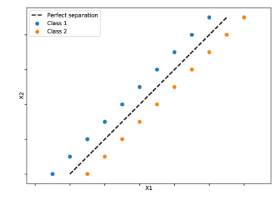
(a) Features are correlated ($\rho(X_{1},X_{2})=0.94$) and not redundant.

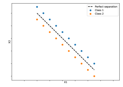
(b) Features are anti-correlated ($\rho(X_{1},X_{2})=-0.94$) and not redundant

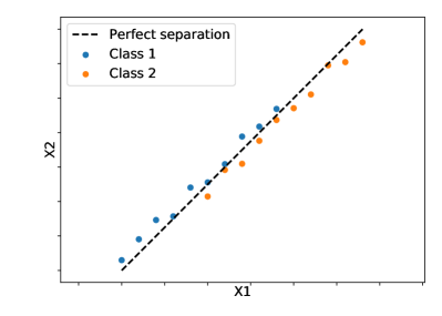
(c) Features are correlated ($\rho(X_{1},X_{2})=0.99$) and not redundant.

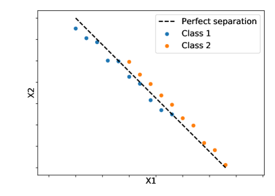
(d) Features are anti-correlated ($\rho(X_{1},X_{2})=-0.99$) and not redundant.

(e) Features are correlated ($\rho(X_{1},X_{2})=1$) and indeed redundant.

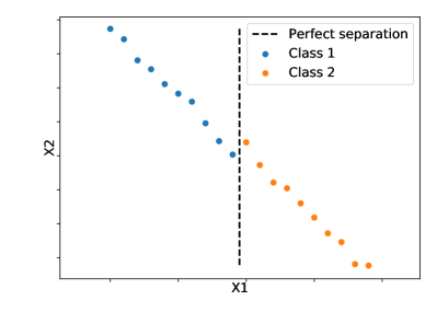
(f) Features are anti-correlated ($\rho(X_{1},X_{2})=-1$) and indeed redundant.

Figure 2.8: Illustrating examples where correlation does not necessary imply redundancy. Figures (a) to (d) show that features can be highly correlated while being not redundant as both features are required to achieve a perfect separation between the two classes. Figures (e) and (f) show that correlated features can indeed be redundant as one feature out of the two is enough to perfectly separate classes. Let us note that in both last examples, both features can individually lead to a perfect separation.

7.4   Feature selection problems

Besides the objective of size reduction, the problem of feature selection usually can take two flavours [guyon2003introduction; nilsson2007consistent; genuer2010variable; kursa2011all]. Typically, those side-objectives guide the feature selection and determine the subset of features that end up being selected.

Many studies (e.g., with microarray gene-expression data [ambroise2002selection] or in drug discovery application [janecek2008relationship]) showed that dealing with small sets of relevant features usually gives better results and facilitate learning accurate classifiers [guyon2003introduction; nilsson2007consistent; kursa2011all].

In presence of many features, it is common that a large number of features are either irrelevant or redundant (to the target). Such variables are in principle not necessary to predict the output and computational performances of supervised learning algorithms can often be optimised by discarding them [yu2004efficient]. Discarding some non-redundant features (with respect to those that are kept), may however be detrimental in terms of accuracy. Furthermore, for some specific learning algorithms, it may actually be beneficial in terms of accuracy to keep some redundant features. Moreover, when sample sizes are small compared to the number of features, it may even become beneficial (in terms of accuracy), to discard some non-redundant features (to decrease overfitting). Usually, as the number of selected features grows, it is expected that the performances of a learning algorithm increases and then decreases. The optimal size for the feature subset being the one that maximises the accuracy [hua2004optimal], the minimal-optimal problem is the first problem of feature selection and consists in finding the smallest optimal subset for a given learning algorithm and a given dataset.

When only accuracy of the learnt predictor is used a criterion to select an optimal subset of features, many weakly relevant features (and sometimes even some strongly relevant one) might be discarded. There is however an interest of identifying all features that are somehow related to the target in order to get a full understanding of the underlying mechanism (e.g., in gene expression analysis [golub1999molecular]). The all-relevant problem is the second approach of feature selection and consists in finding all relevant features.

Those two approaches are usually complementary for a given application. Let us take the example of a medical diagnosis that consists in predicting a disease. The doctor has to evaluate a given number of factors before making his diagnosis. The number of factors has to be as a small as possible to save time and money. Hence, one would want to identify a small set of features that provides the best possible diagnosis. The minimal-optimal approach aims at providing such a feature subset. In different circumstances, for research purposes for instance, the all-relevant approach may be more appropriate. One may want to identify all factors that are related to the output even if some of them are redundant with respect to other.

Both feature selection approaches are further described below.

All-relevant problem

The all-relevant problem is defined as follows [nilsson2007consistent; kursa2011all]:

Definition 2.17.

The all-relevant feature selection problem consists in finding all relevant features. The solution to this problem is the set of all strongly and weakly relevant features.

The solution of this problem is in principle unique, as suggested by Figure 2.9. One further step, in such an analysis, would be to also distinguish between strongly and weakly relevant features.

Figure 2.9: The solution $S$ to the all-relevant problem is the union of weakly relevant and strongly relevant features to the target variable. This set includes all relevant features even if there is redundant information about the target.

Minimal-optimal problem

In terms of learning algorithm performances, the minimal-optimal problem is usually defined as follows [kohavi1997wrappers; nilsson2007consistent]:

Definition 2.18.

Let $\mathcal{A}$ be a learning algorithm, $V$ the set of input features and $Y$ be the target feature. The minimal-optimal feature selection problem consists in finding a subset of $V$ of minimal size that minimises the generalisation error of $\mathcal{A}$.

A solution of this problem is usually a subset of all relevant features, even if for some very specific combinations of problems and algorithms, including irrelevant features may actually be beneficial from the viewpoint of accuracy [kohavi1997wrappers].

For regression and calibrated classification tasks, tsamardinos2003towards showed that a Markov boundary of minimal size is a solution to the minimal-optimal problem (see [tsamardinos2003towards, Proposition 3] for more details and see side note on page 7.4 for a word on Markov blanket discovery algorithms). Therefore, a solution of the minimal-optimal problem is a set made of all strongly relevant and a maximal subset of non-redundant weakly relevant features [kursa2011all]. Let us however note that when the zero-one loss is used (i.e., only the most probable class of $Y$ is required), tsamardinos2003towards state that only some features of the Markov boundary are required or features that do not belong to the Markov boundary.

Markov blanket and boundary discovery algorithms constitute another broad family of feature selection techniques (see, e.g., [guyon2003introduction; tsamardinos2003time; aliferis2010local; statnikov2013algorithms; tsamardinos2003algorithms]). They are usually independent of any learning algorithm and are mainly based on graph theory and related to causality. They are however not addressed in this thesis.

Resulting of the multiplicity of Markov boundaries, the minimal-problem problem does not have a unique solution in general. For example, in presence of two totally redundant features, each can be kept (without the other one) giving two valid options. For strictly positive distributions however, the Markov boundary $M$ of $Y$ is unique and corresponds to the set of all strongly relevant variables [nilsson2007consistent].

Figure 2.10 shows typical solutions to the minimal-optimal problem with respect to the relevance of features. In the case of a strictly positive distribution, Figure 2.10a gives the unique solution to the minimal-optimal problem which is the set of strongly relevant features. In the case of non-strictly positive distribution, Figure 2.10b illustrates a solution to the minimal-optimal problem which includes in all generality some weakly relevant features and all strongly relevant ones.

Finding an optimal subset is usually intractable because some distributions may require an exhaustive search of all possible subsets to guarantee optimality [cover1977possible; kohavi1997wrappers; blum1997selection; yu2004efficient; nilsson2007consistent]. With $p$ features, there are $2^{p}$ possible subsets which is clearly impractical, especially for high-dimensional datasets. However, letting this search be guided by a heuristic (see Section 7.6 and [guyon2003introduction]) or considering only strictly positive distributions [nilsson2007consistent] make this problem more tractable computationally.

(a) Distribution satisfying the intersection property

(b) Distribution not satisfying the intersection property

Figure 2.10: Typical solutions $S$ to the minimal-optimal problem for distributions satisfying the intersection property or not. Solutions are Markov boundaries of $Y$ with respect to $V$.

7.5   Feature selection methods

Feature selection methods are usually classified in three categories depending on how they interact with the learning algorithm: filters, wrappers and embedded methods [blum1997selection; guyon2003introduction; tsamardinos2003towards; saeys2007review].

Filters

A filter approach aims at selecting features independently of the learning algorithm (i.e., without optimising its performance) [kohavi1997wrappers; blum1997selection; guyon2003introduction; guyon2006introduction; saeys2007review; brown2012conditional; chandrashekar2014survey]. A filter tries to assess the interest of keeping features solely from the data in order to then filter out irrelevant features. As a pre-processing step that selects inputs, any learning algorithm can thus be combined with a filtering feature selection.

A common filter method is feature ranking [stoppiglia2003ranking; blum1997selection; guyon2003introduction; chandrashekar2014survey] and consists in ordering features according to a suitable ranking criterion. Any feature relevance measure providing a numerical score can be used (e.g., correlation [guyon2003introduction] or mutual information [blum1997selection; brown2012conditional] with the target, decision tree [cardie1993using], …). Then the top $k$ features (i.e., with highest value) are selected [blum1997selection; saeys2007review; chandrashekar2014survey]. The number $k$ of selected features is determined using an (arbitrary or not) threshold value or based on a random probe (i.e., a random variable is introduced in the process in order to determine which features are statistically better than an artificial irrelevant feature and thus relevant) [stoppiglia2003ranking].

Filter techniques are usually computationally fast and scale very well to high-dimensional datasets [saeys2007review]. As they are independent of the learning algorithm, they only need to be performed once and for all whatever what follows.

A downside of this independence is that filter techniques totally ignore the performance of the learning algorithm with the selected subset [kohavi1997wrappers]. In the filtering approach, most proposed techniques (e.g., correlation and mutual information) are univariate: each feature is considered individually and feature dependencies and redundancies are not taken into account [guyon2003introduction; saeys2007review; chandrashekar2014survey]. Ignoring such effects may lead to a selected set of features that yields poor performance when compared to other types of (multivariate) feature selection techniques [saeys2007review]. Besides, a subset of the selected set of features may be sufficient in presence of redundancy [chandrashekar2014survey]. Consequently, multivariate criteria have been proposed to integrate feature dependencies (e.g., based on mutual information [peng2005feature; meyer2008information; frenay2013mutual; meyer2013information] or based on Markov blankets [koller1996toward], and see [brown2012conditional] for a unifying framework based on conditional likelihood maximisation) but at the cost of scalability and computational speed [saeys2007review].

In the light of the feature selection problems introduced in Section 7.4, two filter approaches are of interest:

the focus algorithm

[almuallim1991efficient; almuallim1991learning; almuallim1994learning] conducts an exhaustive search among all possible subsets of features for the minimal one providing a perfect discrimination (or the best possible) of the target values [koller1996toward; kohavi1997wrappers]. It has a preference for a small set of features and suffer from the so-called Min-features bias [almuallim1991efficient] which may lead to a poor feature selection (see side note on page the focus algorithm). Nevertheless, it is expected that the selected set of features includes all strongly relevant features and some weakly relevant ones.

By chance, an irrelevant feature could be sufficient to perfectly determine the target value in the training data (e.g., a unique sample ID such as the social security number in a medical dataset). A learning algorithm receiving such a feature would surely overfit the training data leading to poor performances in generalisation [kohavi1997wrappers]. A preference towards small set of features - the Min-features bias - would choose that variable as the best subset in comparison with other subsets made of a single variable.

the relief algorithm

[kira1992feature; kira1992practical] is an instance of feature ranking and aims at assigning a relevance score to each feature. The selection is then made by considering as relevant (and thus to be kept) features with a relevance score above a given threshold (determined for instance by a statistical method of interval estimation). The selected subset of features is expected to be the set of all relevant features (weak and strong ones) including redundant features.

Figure 2.11 illustrates a typical solution according to the relevance for both algorithms. One can see that Focus algorithm aims to solve the minimal-optimal problem (although ignoring the usefulness of the selected set of features) and that Relief algorithm aims to solve the all-relevant problem [kohavi1997wrappers].

(a) Focus ($F_{F}$) aims to solve the minimal-optimal problem

(b) Relief ($F_{R}$) aims to solve the all-relevant problem

Figure 2.11: Expected set of features selected by Focus ($F_{F}$) and Relief ($F_{R}$) algorithm according to the feature relevance.

Wrappers

A wrapper method aims at selecting a set of features using a learning algorithm as a "black box" [kohavi1997wrappers; blum1997selection; guyon2003introduction; saeys2007review]. A set of features is presented to a learning algorithm and the corresponding accuracy performances is used as an estimation of the relative usefulness of the given set of features. The search over all possible subsets is usually guided by a search algorithm (see Section 7.6 for more details) "wrapped" around the learning algorithm [saeys2007review]. At the end, the best set of features is then selected as the one leading to the best performances of the given learning algorithm.

In the wrapper approach, the optimal feature subset search is carried out in interaction with a specific learning algorithm $\mathcal{A}$. The resulting selected set of features is therefore the most useful for $\mathcal{A}$ but also tailored to it. Wrapper methods benefit from learning algorithm characteristics (e.g., feature dependencies) but depend on its complexity implying a high computational cost. In contrast with filter techniques, the feature selection is coupled with the learning algorithm performances increasing the risk of overfitting. Examples of wrapper methods (e.g., sequential feature selection and sequential backward elimination) are given in Section 7.6.

Embedded methods

An embedded method of feature selection is comprised in the learning algorithm [blum1997selection; guyon2003introduction; geurts2006extremely; saeys2007review; chandrashekar2014survey]. Similarly to wrapper methods, the selected set of features is specific to the learning algorithm. However, the feature subset search and evaluation are incorporated in the training algorithm [guyon2006introduction] and thus embedded methods are usually less computationally expensive than wrapper methods [saeys2007review; chandrashekar2014survey]. Two examples of embedded methods are two regularised linear regressions known as Lasso and Ridge regressions. Both methods construct a linear model that minimises its error for a given loss function and uses a subset of the variables while including a penalty term that limits the number of variables used. Similarly with wrappers, the selected set of features may depend on the considered embedded method. Indeed, Lasso and Ridge regressions use different penalisation terms and therefore may select different set of features.

7.6   Feature subset search algorithms

Given $p$ features, the number of possible feature subsets (i.e., equal to $2^{p}$) grows exponentially with the number of features making the feature selection space (i.e., the space of all possible subsets of features) very large. Several approaches have been proposed to explore this space. An exhaustive search is optimal but computationally intensive. Heuristic searches have been introduced to explore this space more efficiently. In the rest of this section, we describe well-known search algorithms that will be of interest in this thesis.

exhaustive search

[kira1992feature] consists in exploring the whole feature selection space. All possible subsets are evaluated and the smallest one that maximises a given criterion (which can be a relevance index for a filter approach or the accuracy for a wrapper method for example) is selected. The optimal subset is thus always found at the expense of computational efficiency. For example, the Focus algorithm [almuallim1991efficient; almuallim1991learning; almuallim1994learning] examines subsets by increasing order of size and stops as soon as an optimal subset is found. This approach limits the computational burden while preserving optimality [kira1992feature].

heuristic search

explores more efficiently the search space while trying to find the best (possible) subsets of features. Several approaches aim at reducing the number of subsets to evaluate. A first way consists in limiting the maximal size to $d\leq p$. Only subsets with $d$ or less features are considered but this requires an explicit value of $d$ which is in practice unknown [kira1992feature; devijver1982pattern].

The Sequential Feature Selection (SFS, also known as Forward Selection) [whitney1971direct; miller1990subset; kira1992feature; blum1997selection; jain2000statistical; guyon2003introduction; reunanen2003overfitting; chandrashekar2014survey] starts by selecting the single feature that maximises the given criterion and then sequentially adds one feature at a time. At each step, each remaining feature is evaluated in combination with already selected features and the best one is permanently added to the current subset. The process stops when all features have been added or when the required size of subset is reached. Conversely, the Sequential Backward Elimination (SBE, also known as Sequential Backward Selection) [marill1963effectiveness; kira1992feature; pudil1994floating; kohavi1997wrappers; blum1997selection; jain2000statistical; guyon2003introduction; chandrashekar2014survey] starts with all features and then evaluates shrinking feature sets. At each step, the less promising feature (i.e., the one whose removal is the less penalising according to the criterion) is removed, one at a time, until the required subset size is reached.

SFS is more computationally advantageous than SBE as first evaluated subsets are made of few features [kohavi1997wrappers] (see side node on page 7.6). Feature dependency is not taken into account as some features may not be very useful individually while being highly informative together [kira1992feature; chandrashekar2014survey]. However, the backward elimination strategy can theoretically capture feature interactions [kohavi1997wrappers]. Both approaches do not examine all possible subsets and yield nested feature subsets in the sense that a selected (respectively removed) feature can not be removed (respectively re-selected) even if it would lead to a better subset of features [pudil1994floating; guyon2003introduction; reunanen2003overfitting; chandrashekar2014survey]. Therefore, optimality of the selected subset can not be guaranteed [pudil1994floating; jain1997feature]. More complexed algorithms have been proposed in order to overcome nested subsets. The approach "Plus-$l$-Minus-$r$" consists in combining the forward selection and backward elimination in selecting at each step the $l$ most promising features and removing the $r$ less promising ones [stearns1976selecting; kittler1978feature]. Parameters $l$ and $r$ need however to be fixed. Sequential Floating Forward Selection (SFFS) follows the sequential search procedure but includes a potential feature elimination at each step [pudil1994floating; somol1999adaptive]. Similarly, Sequential Floating Backward Elimination (SFBE) includes a potential feature selection at each step [pudil1994floating; somol1999adaptive]. Adaptive Sequential Forward Floating Selection (ASFFS) generalises above-mentioned approaches with an adaptive determination of $l$ and $r$ at each step [somol1999adaptive].

Let us consider a dataset $\mathbf{D}$ made of a set $F$ of $p$ features and $N$ samples. We want to solve the minimal-optimal problem. Thus, we need to identify the best feature subset of $F$ according to a function $J(E)$ that evaluates a feature subset $E\subseteq F$ on the dataset $\mathbf{D}$. The evaluating function $J$ can either be an independent criterion (in a filtering approach) or an induced model (in a wrapper approach). In both cases, $J$ returns a score that assess the quality of the selected subset $E$ and has a computational cost $\mathcal{O}(J)$ (e.g., that may be the computation cost of the model). In the case of an exhaustive search, all $2^{p}$ subsets must be examined in order to find the best one. The overall complexity is therefore $\mathcal{O}(2^{p})\mathcal{O}(J)$ but guarantees optimality. This can be conceivably performed, if $p$ is not too large [guyon2003introduction] but otherwise it is computationally intractable. In the case of a heuristic search (either SFS or SBE), the complexity is $\mathcal{O}(p^{2})\mathcal{O}(J)$, which is much less than $\mathcal{O}(2^{p})\mathcal{O}(J)$. Both are then much more efficient than exhaustive search but may not yield optimal results as the procedure may miss some feature interactions. It should be stressed that the evaluating function cost may overburden the overall search complexity and therefore it is important to have an efficient and reliable evaluation of each subset. In Chapter 7, we propose to use a computationally inexpensive model (i.e., a randomised tree, see Chapter 3 for a definition) to perform a multivariate sequential feature selection. Let us also mention that nilsson2007consistent showed that if the distribution is restricted to be strictly positive (i.e., all weakly relevant variables are necessarily redundant and thus can be ignored): the minimal-optimal problem can be solved in polynomial time in the number of features and SBE approaches become consistent (but SFS ones do not).

7.7   Discussion

This section aims at reviewing some of the main limitations of feature selection and open problems that motivate some of the research questions considered in the rest of this thesis.

Feature relevance in the context of others

Multivariate approaches are usually preferred over univariate ones because they take into account feature dependencies even though they are computationally less efficient. It shows that feature dependencies is crucial in many applications. Relevant features (even strongly) can be marginally irrelevant while being (highly) relevant in combination with other features [domingos1996exploiting; guyon2003introduction]. A well-known example is the exclusive-OR (XOR) structure [guyon2003introduction; kohavi1997wrappers]. Redundancy (another form of feature dependency) may tone relevance or usefulness of features down. Consequently a feature may be not selected (or identified as relevant) while being highly marginally relevant.

The problem of finding all relevant features requires thus to carefully take into account feature dependencies and the only way to do so is to perform an exhaustive search [nilsson2007consistent], especially to identify weakly relevant features. For example, a sequential forward selection would systematically fail in the identification of relevant features structured such as cliques, i.e. all features are relevant together but are irrelevant in any subset of the clique. Indeed, let us for instance consider a clique made of two features, i.e. an XOR structure. SFS evaluates the relevance of features in the context of already selected ones. In our example, if both features are marginally irrelevant, then none will be selected preventing also the identification of the other feature. SFS is thus unable to identify features that are only relevant in the context of non-selected ones. Nevertheless, features that make other features relevant need to be relevant as well and thus may be end up being selected [sutera2018random]. However, if such structures are excluded (e.g., by considering only PCWT distributions), the exhaustive search is not required any more and the all-relevant problem can be solved efficiently [nilsson2007consistent]. Complex feature structures such as the clique are studied in Chapter 7 in the context of tree-based feature selection.

Last but not least, the confounding effect is an indirect feature interaction. One input feature may seem irrelevant to the target but another feature, an external feature known as a confounding factor, provides the key to understand the relationship between the input feature and the output. This confounding effect can be enlarged to features that appear at first sight to be irrelevant but, taking into account the context, are indeed relevant. Such feature interactions are studied in Chapter 6.

Feature ranking is limited for interpretation

Feature ranking is extremely limited as it only provides a single ordering of features. This ranking can not render the full complexity of feature interactions or the multiplicity of optimal subsets of features. The subset evaluation function is also critical, e.g. a univariate criterion will only rank features according to their marginal relevance missing potential interactions.

In all generality, the most relevant features are not necessary the best ones (or the only ones) to select [guyon2003introduction]. The top-ranked feature may be a rather good feature to predict the target but some other features with lower ranks may perfectly discriminate the target together. Redundancy may have lowered the rank of redundant but highly relevant features [guyon2003introduction]. Selecting a top-ranked feature may also be counter-productive, e.g. selecting only one feature of a clique is not interesting without all the rest of the clique (which might typically be much lower in the ranking). Although very useful, feature selection/ranking methods however only provide very limited information about the often very complex input-output relationships that can be modelled by supervised learning methods. There is no information about feature dependencies in a classical feature ranking. In case of a contextual effect, two similar ranked features may have totally different roles. One may be always relevant while the relevance of the other one depends on the context. The interpretation is totally different but the rank similarity seems to indicate that they are similarly relevant as well.

Feature ranking does not allow to distinguish among features that are directly related to the output and those that influence it only indirectly. Applications focusing on direct links (e.g., network inference [de2010advantages; huynh2010inferring; altay2011differential; marbach2012wisdom], see also Chapter LABEL:ch:connectomics), must therefore filter out the indirect component from feature selection methods.

There is thus a high interest in designing new techniques to extract more complete information about input-output relationships than a single global feature subset or feature ranking. A first step towards more interpretable results could be to derive more than one (relevance) score to capture the interest of a feature in several settings. Chapter 6 extends classical tree-based feature ranking to incorporate a contextual analysis.

Finite sample size makes feature selection more difficult

High dimensionality together with small sample-size are nowadays typical in many application domains and it poses a great challenge for classical machine learning techniques [raudys1991small; braga2004cross; molinaro2005prediction; saeys2007review] and in particular for feature selection [sima2006should; saeys2008robust; meinshausen2010stability; kuncheva2007stability; bolon2015recent; kuncheva2018feature]. In such conditions, feature selection is however all the more interesting and may help, for example, to counter-balance the disadvantageous features/samples ratio by reducing the number of variables. Nevertheless, studies show that selecting features in such datasets (e.g., micro-arrays of gene-expression) is less reliable [jain1997feature; sima2006should]. In this case, feature selection methods may not necessarily provide a close-to-optimal feature set (i.e., whose error is close to the minimal achievable error) [sima2006should; hua2009performance]. They also may be unable to find a satisfying feature subset and this does not imply either that an optimal subset does not exist [sima2006should; hua2009performance].

Despite an expensive computational cost, the evaluation function must be properly (cross-)validated to avoid the risk of overfitting and overestimated accuracy performances (known as the so-called "peeking phenomenom" or as "selection bias" problem [ambroise2002selection]) [reunanen2003overfitting; smialowski2009pitfalls; pereira2009machine; diciotti2013peeking; kuncheva2018feature]. Hybrid data (i.e., coexistence of categorical and numerical data) are also worthy of attention [wang2016efficient; jiang2016efficient].

In small sample-size conditions, small changes (e.g., addition/removal of samples or noise added to features [saeys2008robust]) may have a strong influence on the selected feature subset. For the sake of interpretation for instance, one would usually prefer some stability in the outcomes of feature selection algorithm. In a cross-validation feature selection, this would be highly undesirable to have tremendously different selected feature sets from two folds drawn from the same dataset. Stability of feature selection with respect to sampling variation have drawn researchers’ attention as another step towards a more robust feature selection [kuncheva2007stability; kalousis2007stability; saeys2008robust; saeys2008towards; abeel2009robust; he2010stable].

In small sample-size conditions, irrelevant variables may seem relevant due to random fluctuations. Indeed, the risk of having spurious associations between irrelevant features and the output increases with a decreasing sample-size, especially if the number of features is large [kursa2011all]. Discerning barely but truly relevant from falsely relevant features is a common issue in feature selection with high-dimensional datasets. Solutions, such as introducing an artificial random contrast variable [stoppiglia2003ranking; tuv2006feature; rudnicki2006statistical; kursa2011all; huynh2012statistical] or using dimensionality reduction techniques (by random projections, see random subspace method [ho1998random] in Chapters 3 and 7), are required to do so.

Decision trees and ensemble methods

“May the forest be with you.”

8   Introduction

A popular and classical approach to solve a complex problem is the divide-and-conquer strategy. It consists in (recursively) dividing the problem into several sub-problems easier to solve. The solution of the original problem is then a combination of the sub-problem solutions. Based on that strategy, the recursive partitioning method aims at simplifying a task to carry out on a set of elements (e.g., sorting, labelling, …) by recursively dividing the set into smaller and smaller subsets in such a way that doing this task is easier in each subset than in the original set. For example, sorting can be achieved efficiently using this strategy: the merge-sort algorithm recursively divides the list of elements into smaller and smaller groups until each sub-group is easy (or trivial) to sort, and then combines sorted sub-lists.

The decision tree algorithm successfully applies this method to provide a supervised learning model that partitions the input space into distinct (smaller) subspaces [breiman1984classification; quinlan1986induction; quinlan2014c4]. As a sub-problem, an output value is then assigned to each subspace. From there, the prediction of a new object simply consists in identifying the subspace in which it falls to retrieve its predicted output value.

Single decision trees are simple and consistent supervised models making them easy to use and to understand. They however suffer from variance, and their accuracy performances are consequently affected.

In order to circumvent variance issues and thus improve model performances, ho1998random; dietterich2000experimental; breiman2001random were among the firsts to propose to grow an ensemble of trees instead of settling for a single one. Making a prediction by letting every tree vote and then aggregating these votes results in significant improvement in accuracy. Many state-of-the-art algorithms stemmed from that idea, including random forests and boosting methods. In particular, a random forest is an ensemble (i.e., a forest) of randomised trees and is at the centre of this thesis. Randomisation is introduced to create some diversity between trees of the same ensemble. The motivating assumption of this approach is that the prediction of an ensemble of weak models is better than the prediction of a single (supposedly stronger) model.

Furthermore, the success of tree-based methods is also explained by their following common characteristics [geurts2002contributions; louppe2014understanding]:

non-parametric nature

by not requiring a priori assumptions on the relationships between inputs and output,

ability to handle heteregeneous data

by handling learning sets made of a mix of continuous, discrete (ordered or not), and categorical variables (but not necessarily fairly, see Section 14.5.3 for more details),

robustness to outliers or errors in labels

by usually avoiding to completely modify the model to fit a few spurious values in the data,

robustness to irrelevant or noisy variables

by automatically selecting the most useful (and relevant) features to build the tree structure (at least to some extent, see Chapters 4 and 5 for more details),

interpretability

by providing a decision path (with decision trees) or an importance degree for used features (with ensemble methods, see Chapters 4 and 5 for more details),

In this chapter, Section 9 describes the decision tree algorithm. Then, Section 10 presents ensemble methods as a way of circumventing the high variance of decision trees.

9   Supervised Learning with Decision trees

9.1   Semantics of tree based prediction models

9.1.1   From graph theory to decision tree terminology

In all generality, let $G=(V,E)$ be a graph where $V$ is a finite set of nodes $t$ (also denoted as vertices in graph theory), and $E\subset V\times V$ is the set of edges. The graph is called undirected, if $(t_{i},t_{j})\in E$ implies that also $(t_{j},t_{i})\in E$. In graph theory, a tree is an undirected graph in which any two vertices are connected by exactly one (undirected) path.

We use the term tree structure to denote a directed graph obtained from a tree by choosing a node as the root (denoted $t_{0}$), and by directing all edges ‘away’ from this root (see Figure 3.1 for an illustrative example). A branch $(t_{i},t_{i+1})$ is an edge going from $t_{i}$ towards $t_{i+1}$ where $t_{i}$ is called the parent of $t_{i+1}$, and $t_{i+1}$ is a child of $t_{i}$. A node is internal if it has at least one child, and terminal (also known as leaf node in the tree terminology) if it has no children.

Figure 3.1 gives an example of a tree structure (i.e., a tree-structured graph). It is represented with the (internal) root node $t_{0}$ on top and such that nodes at the same depth (i.e., distance with respect to the root node) are horizontally aligned. Nodes $t_{1}$ and $t_{2}$ are also internal because they respectively have the children $t_{3},t_{4}$ and $t_{5},t_{6}$. Here $t_{3},t_{4},t_{5},t_{6}$ are the leaves of the tree.

The following section describes a decision tree model: a tree structure with an additional layer of information.

Figure 3.1: Example of a tree-structure.

9.1.2   A tree structure shaped by the features

A tree structure $G_{T}$ recursively partitions the input space $\mathcal{X}$ into subsets where each node $t$ is associated to one specific subset $\mathcal{X}_{t}$. The subsets corresponding to the terminal nodes are disjoint and such that their union is the original input space $\mathcal{X}$, i.e., $\cup_{t\,\text{is terminal}}\mathcal{X}_{t}=\mathcal{X}$. The subset corresponding to an internal node is the union of the subsets attached to its children; hence the subset corresponding to the root is always the whole input space. To define all these subsets the tree structure uses features as building blocks. Each internal node typically uses one specific feature, in order to partition its own subset into the subsets corresponding to its children.

In all generality, a split $s$ is a partition of a set $\mathcal{L}$ into a finite number of non-empty and disjoint subsets $\mathcal{L}^{i}$. In other words, every element of $\mathcal{L}$ belongs to one and only one $\mathcal{L}^{i}$. A split on a node $t$, also known as a test and denoted by $s_{t}$, is a split of $\mathcal{X}_{t}$ using the value of a feature to compute the partition. A split variable $v(s_{t})$ is the variable on which the test $s_{t}$ is based and is the one that corresponds to node $t$ in the tree structure.

The cardinality of a split $s_{t}$, denoted $|s_{t}|$, corresponds to the number of created subsets, or equivalently the number of possible test outcomes. Cardinalities may or may not be the same for all $t$. The cardinality $|s_{t}|$ also determines the number of children of node $t$ (i.e., the node cardinality) and may depend on the number of possible values for the split variable (the variable cardinality).

A split is said to be binary if exactly two subsets are created. However, a node can be divided in more than two by a so-called multiway splits. A multiway split is said to be exhaustive if the split cardinality is equal to the number of values of the split variable (i.e., one value per branch).

Some authors have looked at more exotic splits. An oblique split is made by using a linear combination of several numerical features to create the partition. In an even more general framework, multivariate splits also consider complex models (e.g., a decision tree [botta2013walk]) as separating functions, extending axis-parallel and oblique splits [gama2004functional]. Fuzzy trees do not longer consider disjoint subsets for children but take advantage of the fuzzy logic to allow some (uncertain) samples to be in several terminal nodes [janikow1998fuzzy; olaru2003complete].

Figure 3.2: Example of a decision tree model: a tree-structure that recursively splits the $2\times 2$ input space with four colours.

9.1.3   Decision tree models

A decision tree model $T:\mathcal{X}\rightarrow\mathcal{Y}$ recursively partitions the input space $\mathcal{X}$ into subspaces to provide an input-output model in the form of a tree structure (see Figure 3.2 for an illustrative example). The model is such that

1. each node $t$ corresponds to one subset $\mathcal{X}_{t}\subseteq\mathcal{X}$, in particular the one associated to the root node is the input space $\mathcal{X}$ itself,

2. each internal node $t$ is labelled with a split $s_{t}$,

3. each branch going from an internal node $t$ indicates one possible outcome $i$ of the split $s_{t}$, and leads to one child $c_{i}$ of $t$ such that its subset is $\mathcal{X}_{c_{i}}=\mathcal{X}_{t}\cap\mathcal{X}^{i}$ where $\mathcal{X}^{i}\subset\mathcal{X}$ is the subset of inputs satisfying outcome $i$,

4. all terminal nodes $t$ have their subsets (called terminal subsets) assigned to a predicted value $\hat{y}_{t}\in\mathcal{Y}$; $\hat{y}_{t}$ is also called the label of the leaf $t$.

Figure 3.2 shows a decision tree model that decomposes an input space of two dimensions (represented by a $2\times 2$ matrix) with four possible output values (i.e., green, blue, red, or orange) using the tree-structure of Figure 3.1. The root node $t_{0}$ corresponds to the complete input space $\mathcal{X}$. Its split is made on the vertical axis ("Which row?") and gives two children ($t_{1}$ and $t_{2}$) corresponding to the two possible outcomes (i.e., top or bottom). Each child has its own subset that is still made of two colours. By splitting them on the horizontal axis ("Which column?"), we obtain four terminal nodes, each with a subset of only one colour. At this point, there is no interest in further partitioning these subsets. The output label associated to each terminal node is immediate and corresponds to the remaining colour. The prediction of the model for a new input value $\mathbf{x}$ is the associated value of the terminal node reached by $\mathbf{x}$. Let us observe that, for each internal node $t$, the input subsets of its children are disjoint and their union is the subset of that node $t$, i.e., $\mathcal{X}_{t}=\cup_{i=1}^{|s_{t}|}\mathcal{X}_{c_{i}}$.

Let us consider a more realistic classification problem, described in Example 3.1, that will be used to illustrate the two following decision tree models.

Example 3.1.

Let us consider a classification problem with two input variables $X_{1}$ and $X_{2}$ with two possible output classes $c_{1}$ and $c_{2}$. Figure 3.3 illustrates the learning set where each input variable corresponds to one dimension. At first sight, based on Figure 3.3a, this is not straightforward to give a model that will perfectly separate the two classes. For the sake of illustration, Figure 3.3b gives a decomposition of the input space that provides a perfect separation between objects of different classes.

(a) Raw data

(b) Explained data

Figure 3.3: Example of a classification problem with two input variables $X_{1}$ and $X_{2}$ and two possible values of the output $y$ ($c_{1}$ and $c_{2}$). Blue dots correspond to objects class $c_{1}$ while orange squares correspond to objects class $c_{2}$. On the right figure, the underlying decomposition of the input space is explicitly given.

Definition 3.1.

A binary decision tree is a decision tree model in which all internal nodes have exactly two children.

This is the case when all splits are binary, that is to say, when there are only two possible outcomes (e.g., true or false, yes or no), or when all input features are binary.

A split $s$ divides the input space between the part that satisfies the test $\mathcal{X}^{s}$ and the rest $\mathcal{X}^{\bar{s}}$. Therefore, the input subspace of the left child $c_{l}$ of $t$ (i.e., satisfying the test) is $\mathcal{X}_{c_{l}}=\mathcal{X}_{t}\cap\mathcal{X}^{s}$ , and the input subspace of the right child $c_{r}$ is $\mathcal{X}_{c_{r}}=\mathcal{X}_{t}\cap\mathcal{X}^{\bar{s}}=\mathcal{X}_{t}\cap(\mathcal{X}\setminus\mathcal{X}^{s})$.

Figure 3.5 shows a binary classification tree applied on Example 3.1.

Figure 3.4: Example of a binary classification tree applied on Example 3.1.

Figure 3.5: Example of a multiway classification tree applied on Example 3.1.

Decision trees are typically binary but they can also be built using multiway splits. Figure 3.5 illustrates a multiway decision tree applied on Example 3.1. In comparison with the binary decision tree of Figure 3.5, threeway splits are used at the second level to create three children corresponding to three intervals of values of $X_{1}$ (in the example, intervals $[0,1],]1,2],]2,3]$). Notice that while the binary tree uses two more splits, it manages to find the same final partition.

When all input variables are categorical, let us define a decision tree using multiway exhaustive splits:

Definition 3.2.

Let all input variables $V=\{X_{1},\dots,X_{p}\}$ be categorical. A multiway exhaustive decision tree is a decision tree model in which splits on feature $X_{i}$ yield exactly $|X_{i}|$ children, namely one for each possible value of the split variable $X_{i}$.

Multiway exhaustive splits are typically of various cardinalities as they depend on the number of possible values of each split variable. Notice that for such a tree, the maximal depth is limited by the number of features, as each feature can be used at most once along a path.

9.2   Learning a decision tree model from data

The tree model aims at fitting at best the partition induced by $\mathcal{Y}$ over $\mathcal{X}$ and thus approximating the Bayes model (i.e., the optimal model yielding the lowest error rate). In practice, the partition induced by $\mathcal{Y}$ over $\mathcal{X}$ is unknown and the input space is only partially observed through a learning set. Given a learning set $\mathbf{LS}$, a decision tree model $T^{\mathbf{LS}}$ is learnt on $\mathbf{LS}$ and provides a partitioning of $\mathbf{LS}$, denoted $\varphi$. While growing the decision tree, the objective is to find the partitioning $\varphi$ that provides the lowest possible error rate, the optimal induced partitioning $\varphi^{*}$. Assuming that the learning set represents faithfully the input space, $\varphi^{*}$ should be close to the partition induced by $\mathcal{Y}$ over $\mathcal{X}$.

The tree learning algorithms that we consider in this thesis (and which have become a standard in supervised learning) proceed in a top-down fashion, by starting with the root node and progressively developing the tree structure, while at each step choosing a node to split and a way to split the node, until the tree fits the learning sample sufficiently well (see side note on page 9.2).

$\bullet$ Initialization: create the root node of the tree, attach the whole learning set to this node, and set the list of open nodes to contain only this node. $\bullet$ Recursion: until the list of open nodes is empty, remove a node from the list of open nodes (following a given growing strategy), and decide whether this node should be split: – If yes, the node becomes a test node, and a good split for it is determined and used to split the learning set of the node into two or more subsets. For each subset a child node is created and inserted in the list of open nodes. – If no, the node becomes a leaf and a class label is assigned to it based on its learning subset.

This procedure aims at finding a suitable tree structure, and at associating the right class label to each one of its terminal nodes. This thought has been summarised by breiman1984classification as follows:

“It turns out that the class assignment problem is simple. The whole story [of the construction of a tree] is in finding good splits and in knowing when to stop splitting.” [breiman1984classification]

The three next sections are dedicated to a detailed description of these three key steps of a decision tree learning procedure. In Section 9.2.1, we describe how to find the variable (and the associated test) that provides a "good" split for a learning subset. In Section 9.2.2, we review some stopping criteria that define the end of the building process. In Section 9.2.3, how to choose the labels attached to leaves and used for making predictions.

9.2.1   Splitting rules

The impurity framework

The growing/learning procedure of a decision tree model recursively divides the learning set in subsets of learning samples $\mathbf{LS}_{t}$ where $\mathbf{LS}_{t}$ is the set of all objects reaching node $t$ (i.e., $\mathbf{LS}_{t}=\{(\mathbf{x},y)|\mathbf{x}\in\mathcal{X}_{t}\}$). For a given node $t$ and its set of learning samples $\mathbf{LS}_{t}$, let us define $p(c_{j}|t)$ as the proportion of samples in $\mathbf{LS}_{t}$ such that $y=c_{j},\,c_{j}\in\mathcal{Y}$. The sum of $p(c_{j}|t)$ for all $c_{j}\in\mathcal{Y}$ is $1$. Based on $\mathbf{LS}$, the learnt model tries to mimic the optimal induced partitioning $\varphi^{*}$.

A good decision tree is one that minimises the generalisation error while minimising some complexity criterion of three, e.g., the size of the tree. Even though several trees can equivalently represent the optimal partitioning $\varphi^{*}$, the shorter tree is usually the easiest to interpret and consequently the best one. Naively, one can generate all possible decision trees in order to keep the best one (minimising a criterion depending on the accuracy performances and the complexity of the model). However, even if the number of trees may be finite when the number of (discrete/categorical) features is limited, this number can increase exponentially and becomes intractable from a computational point of view when considering a large number of (continuous) features.

Circumventing the intractability of an exhaustive search for the optimal tree model (giving $\varphi^{*}$), the idea of breiman1984classification’s heuristic algorithm is to keep splitting nodes until they are (almost) pure. The resulting partitioning is expected to be close to $\varphi^{*}$. A node $t$ is pure when all learning samples reaching that node ($\mathbf{LS}_{t}$) are of the same class label $c_{j}$ ($p(c_{j}|t)=1,\,c_{j}\in\mathcal{Y}$ and $p(c_{i}|t)=0$ for all $c_{i}\neq c_{j}$,$c_{i}\in\mathcal{Y}$) (see terminal nodes of Figures 3.2, 3.5 and 3.5). Hereafter, we refer to the output distribution of a pure node as a pure distribution. A pure node is always terminal because there is no gain in splitting more its samples. Conversely, the impurity of a node is the largest when all class labels are equally likely ($p(c_{j}|t)=p(c_{i}|t)$ for all $c_{i},c_{j}\in\mathcal{Y}$).

From that, one can logically assume that the purer a node is, the more striking is the majority class making the prediction easier and usually better.

Following the framework of breiman1984classification, let us define an impurity measure $i(t)$ as a non-negative function $\phi$ that evaluates the purity of a node $t$ from the vector of class proportion samples $\pi$ (where the $j^{th}$ term of $\pi$, $\pi^{j}=p(c_{j}|t)$) and verifies the following three properties [breiman1984classification; joly2017exploiting]:

1. $i(t)$ is minimal (typically equal to $0$) when the node $t$ is pure, i.e., $p(c_{j}|t)=1$ for some $c_{j}\in\mathcal{Y}$ and $\forall c_{i}\neq c_{j}:p(c_{i}|t)=0$,

2. $i(t)$ is maximal only when the distribution of output values in $\mathbf{LS}_{t}$ is uniform, i.e. such that $p(c_{i}|t)=\frac{1}{|\mathcal{Y}|}$ for any $c_{i}\in\mathcal{Y}$,

3. $i(t)$ is not biased towards some output values (symmetrical with respect to the class proportion samples), e.g., the impurity measures of two nodes $t_{1}$ and $t_{2}$ are the same if $\pi_{2}$ is a permutation of $\pi_{1}$.

The goodness of a split

A good split is one that reduces the impurity $i(t)$ of a node $t$, i.e., such that children of $t$ are purer than $t$ itself. The goodness of a split dividing a node $t$ in two can be formalised using the impurity measure as follows:

Definition 3.3.

Let $s$ be a binary split that divides a node $t$ into a left node $t_{L}$ and a right node $t_{R}$. The decrease of impurity is

$${\Delta{i(s,t)}} = i(t)-\dfrac{N_{t_{L}}}{N_{t}}i(t_{L})-\dfrac{N_{t_{R}}}{N_{t}}i(t_{R})$$ (3.1)

$$= i(t)-p_{t_{L}}i(t_{L})-p_{t_{R}}i(t_{R})$$ (3.2)

where $N_{t}$ is the number of learning samples in node $t$, $N_{t_{L}}$ and $p_{t_{L}}$ (respectively, $N_{t_{R}}$ and $p_{t_{R}}$) are the number of samples and the proportion of samples that fall into $t_{L}$ (resp., $t_{R}$).

We will discuss later on several impurity measures that may be used for growing decision trees. Once the impurity is chosen, the greedy procedure for growing a decision tree consists in searching at each node for the split that yields locally the largest decrease of impurity $\Delta i(s,t)$ among all valid splits.

Candidate splits for different types of features

Let $S_{t,m}$ be the set of all candidate splitting functions for node $t$ on feature $X_{m}$, consisting of all candidate ways to divide $\mathcal{X}_{t,m}$ in two non-empty subsets, where $\mathcal{X}_{t,m}$ denotes the set of all values of $X_{m}$ observed in the learning sample of node $t$.

If $X_{m}$ is an unordered variable, defining a split amounts to find two non-empty subsets $\mathcal{X}_{t_{L},m}$ and $\mathcal{X}_{t_{R},m}$ such that every element of $\mathcal{X}_{t,m}$ is in one and only one of them, i.e., $\mathcal{X}_{t,m}=\mathcal{X}_{t_{L},m}\cup\mathcal{X}_{t_{R},m}$ and $\mathcal{X}_{t_{L},m}\cap\mathcal{X}_{t_{R},m}=\emptyset$. In that case, $S_{t,m}$ can be formally defined as follows:

$$S_{t,m}=\{s(\mathbf{x})=\mathbb{1}(x_{m}\in\mathcal{X}_{t_{L},m})|\mathcal{X}_{t_{L},m}\subset\mathcal{X}_{t,m}\}$$ (3.3)

where $\mathbf{x}$ is a vector of input values and $x_{m}$ is the value of $X_{m}$. All splits guide samples whose value $x_{m}$ is in $\mathcal{X}_{t_{L},m}$ in the left child, while all others go in the right child. Let us note that $\mathcal{X}_{t_{L},m}$ must be non-empty, and a proper subset of $\mathcal{X}_{t,m}$ to ensure that $\mathcal{X}_{t_{R},m}$ is also non-empty. A combinatorial analysis gives that the number of possible splits $|S_{t,m}|$ is equal to $2^{|X_{t,m}|-1}-1$ where $|X_{t,m}|$ is the cardinality of $X_{t,m}$.

If $X_{m}$ is an ordered variable, the logic between values should be preserved by the split. Consequently, the two disjoint non-empty subspaces $\mathcal{X}_{t_{L},m}$ and $\mathcal{X}_{t_{R},m}$ must be such that every element in one subspace has a split variable value strictly lower than the split variable value of any element from the other subspace, i.e., $\mathbf{x}_{t_{L},m}<\mathbf{x}_{t_{R},m}$ for all pairs $(\mathbf{x}_{t_{L}},\mathbf{x}_{t_{R}})\in\mathcal{X}_{t_{L},m}\times\mathcal{X}_{t_{R},m}$. An equivalent way to fulfil that condition is to determine a threshold value $\tau$ (also called cut-point), and to assign every value below $\tau$ to the left child and to the right child otherwise, i.e.:

$$S_{m}=\{s(\mathbf{x})=\mathbb{1}(x_{m}\leq\tau)|\tau\in\mathcal{X}_{m}\}$$ (3.4)

where $\tau$ is a threshold value referred to as the cut-point of the split.

In practice, it suffices to consider a single candidate cut-point between each pair of successive values of the concerned feature observed in the learning subset of the node $t$ (in most implementations it is the mid-point). Indeed, different cut-points between a given pair of such successive values yield the same partition of the learning sample of the considered node, and are thus equivalent from the viewpoint of impurity reduction. The number of different splits to consider is thus $|S_{t,m}|=|X_{t,m}|-1$. Let us however notice that all cut-points between two successive values (as observed in the learning set) are not necessarily equivalent outside the learning set (see Figure 3.6 for an illustrative example).

Figure 3.6: Split selection. Projection on the $X_{1}$ axis of samples reaching the second node that splits on $X_{1}$ (i.e., $X_{1}\leq 2$) on the left branch (i.e., $X_{2}\leq 1$) of the decision tree of Figure 3.5. Filled circles and squares are samples from the learning set $\mathbf{LS}$ and non-filled ones are samples from the testing set $\mathbf{TS}$ (unknown in the learning phase). In practice, all cut-points in the red zone (i.e., between two successive values $]1.7,2.3[$) are equivalent on the learning set and $\tau=2$ was chosen in Figure 3.5. However, other values such as $\tau=1.8$ or $\tau=2.2$ also perfectly separate classes in the learning but not on the test set.

Let $S_{t}$ be the set of splits on all $p$ features and such that $S_{t}=\cup_{j=1}^{p}S_{t,j}$. The best split $s_{t}^{*}$ is therefore

$${s_{t}^{*}=\operatorname*{arg\,max}_{s\in S_{t}}\Delta i(s,t).}$$ (3.5)

In practice, Equation 3.5 is solved by exhaustively considering all features and all possible splits on those features (either all cut-points $\tau$ or all subsets $\mathcal{X}_{t_{L},m}$). This approach however only optimises the split for the current node. Growing a decision tree while foreseeing some future splits is known as (limited) lookahead search and has been shown to provide shorter but not significantly better trees while being computationally more costly [murthy1995lookahead; louppe2014understanding].

Suitable impurity measures

Any function satisfying the three properties of an impurity measure can be plugged in the decision tree algorithm. Classical impurity measures used for classification problems are the Shannon entropy and the Gini index.

Definition 3.4.

The impurity function $i_{h}(t)$ of a node $t$ derived from Shannon entropy [shannon1949mathematical] is

$$i_{h}(t)=-\sum_{j=1}^{C}p(c_{j}|t)\log_{2}(p(c_{j}|t))$$ (3.6)

where $C$ is the number of possible classes.

Shannon entropy quantifies the uncertainty of a discrete random variable based on its probability density. It is non-negative, maximal for a uniform density, and equal to zero (hence minimal) when only one value has a strictly positive probability. Notice that the entropy-based impurity reduction $\Delta i_{h}(s,t)$ is actually an estimation, based on the learning subset reaching the node $t$, of the mutual information between the split outcome and the output $t$. This impurity reduction is also non-negative, and equal to zero only if the class proportions in the two subsets are identical.

Definition 3.5.

The impurity function $i_{g}(t)$ of a node $t$ derived from Gini index [gini1912variabilita] is

$$i_{g}(t)=\sum_{j=1}^{C}p(c_{j}|t)(1-p(c_{j}|t))$$ (3.7)

where $C$ is the number of possible classes.

The Gini index quantifies the dispersion of a distribution. The gini-based impurity $i_{g}(t)$ aims at evaluating the error rate of a random labelling of objects from $\mathbf{LS}_{t}$ following the distribution of labels within node $t$, $p(y|t)$. That is, the probability of labelling an object with class $c_{j}$ is given by the probability $p(c_{j}|t)$ while $1-p(c_{j}|t)=\sum_{i\neq j}^{C}p(c_{i}|t)$ is the probability of error when labelling an object $c_{j}$. Similarly to Shannon entropy, $i_{g}(t)$ is non-negative, maximal for a uniform distribution, and equal to zero and hence minimal for a pure distribution. The resulting impurity reduction is also non-negative, and equal to zero only if the class proportions in the two subsets are identical.

Extension to regression trees

In order to extend the tree growing algorithm to the case where the output is numerical (i.e. for regression), various alternative goodness of split measures have been defined in the literature. In particular, for ’least squares regression’, a natural way to do this is to use the same approach as above while using as “impurity” measure the variance of the output $Y$ estimated from a learning subset [breiman1984classification].

Definition 3.6.

The “impurity” function $i_{v}(t)$ of a node $t$ derived from the variance is

$$i_{v}(t)=\dfrac{1}{N_{t}}\sum_{y\in\mathcal{Y}_{t}}(y-\bar{y}_{t})^{2}$$ (3.8)

where $N_{t}$ is the number of learning samples in node $t$ and $\bar{y}_{t}=\dfrac{1}{N_{t}}\sum_{y\in\mathcal{Y}_{t}}y$ is the average of $y$ in $\mathbf{LS}_{t}$.

The variance estimate $i_{v}(t)$ is non-negative and equal to zero when all samples have the same target value (equal to the mean value). It also leads to an impurity reduction measure that is non-negative.

9.2.2   Stopping rules and pruning

In the previous section, we described how to develop a tree by starting with its root node and splitting its nodes so as to maximise at every step the impurity reduction.

Given the recursive nature of the growing process, there comes a stage when it is no longer possible to further divide a sample set. The splitting process then has no choice but to stop if there is no more valid splits for the node. It occurs in the two following situations, seen as inherent stopping criteria:

1. Constant output value: all learning observations reaching the node have the same output value, meaning that the impurity of the learning subset is already equal to zero and hence can not be further reduced,

2. Constant input values: all learning observations reaching the node have the same value for every input feature, so that the set of available candidate splits is empty.

Let us note that all learning samples may have the same input values (case (b)) while not having the same output value.

Definition 3.7.

A decision tree is said to be fully developed if all learning subsets corresponding to its leaves have either a constant output (case (a)) or constant inputs (case (b)) and consequently none of the leaves could have been split in a meaningful way.

Fully developed trees are often overfitting the training data. To limit this phenomenon, additional criteria for stopping to split have been imposed.

1. Complexity-based stopping criteria aim at preventing the decision tree from becoming too complex. Typical complexity measures are the total number of nodes or the maximal (or average) depth of the tree.

2. Impurity-based stopping criteria stops the growing procedure when the possible impurity reduction is not significant anymore. Indeed, since the growing procedure recursively splits the learning set, the number of learning samples reaching deeper nodes decreases typically rather quickly with the tree depth. Deeper nodes therefore typically yield impurity reductions that are less and less significant from a statistical point of view. Thus it has been proposed to stop splitting if

   1. the size of the learning subset of a node is below a given threshold, or if learning subset sizes of its child nodes would be below a given threshold,

   2. if the best achievable impurity reduction is too small given the size of the learning subset. Instead of setting explicitly a threshold, some statistical measures (e.g., a $\chi^{2}$ test or a permutation test) can associate a split impurity reduction to a significance level (e.g., a p-value) for which it is easier to find an interpretable threshold value.

It should be noted that a single criterion may be sufficient to stop the construction of a tree although several can be combined. In practice, all criteria are defined by a hyper-parameter whose value must be carefully chosen. By being too restrictive with their values, these criteria would result in a shallow tree that potentially misses some information about the output in the dataset (i.e., a situation of under-fitting). On the other hand, choosing parameter values that are too permissive would not limit the size of the tree enough, causing over-fitting and sub-optimal performances (in terms of generalisation error). All parameters must therefore be carefully tuned in order to achieve the best trade-off for the size of the tree.

Although those stopping criteria may give in practice good results, they may also lead to sub-optimal trees. A few nodes more or less might indeed sometimes produce a significantly better tree. Another way of finding the best model is to first build a fully developed tree and then choose one of its subtrees a posteriori. Techniques following this approach are known as post-pruning methods. In practice, a post-pruning method consists in finding the best subtree $T^{*}\subseteq T$, obtained by contracting an internal node of the fully developed tree $T$ (i.e., replacing it by a terminal node and dropping all its descendent nodes), say one which minimises a given criterion such as the error rate on a independent test set for example.

Therefore, stopping criteria that preventively control the growing of the tree are usually referred to as pre-pruning methods.

9.2.3   Labeling the leaves

The prediction $T(\mathbf{x})=\hat{y}(\mathbf{x})$ for an input vector $\mathbf{x}$ is obtained by propagating $\mathbf{x}$ through the tree (following branches according to its values) and then returning the prediction (or label) $\hat{y}_{t}$ associated to the terminal node reached by $\mathbf{x}$.

During the learning stage, each terminal node $t$ must thus receive a label $\hat{y}_{t}\in\mathcal{Y}$. The choice of $\hat{y}_{t}$ of course aims at maximizing accuracy and hence essentially depends on the nature of the output variable and on the loss function used to measure accuracy. In practice the output label values found in the learning subset of each leaf are used to choose a label such that in the end the total loss is minimised over the learning set.

For classification trees and zero-one loss

Let us consider a decision tree model to predict $\mathcal{Y}=\{c_{1},\dots,c_{J}\}$. If the goal is to minimise the probability of mis-classification, the label $\hat{y}_{t}$ associated to a terminal node $t$ is chosen as the most frequent class (output value) among objects reaching node $t$. That is

$$\hat{y}_{t}=\operatorname*{arg\,max}_{c_{j}}p(c_{j}|t).$$ (3.9)

Indeed, in classification tasks, the commonly used loss is the zero-one loss, which for a decision tree and its learning set sums up to

$$L^{0-1}=\sum_{t}\sum_{(\mathbf{x}^{i},y^{i})\in\mathbf{LS}_{t}}\mathbb{1}(y^{i}\neq\hat{y}_{t}),$$

where the outer sum is over all leaves of the tree. And thus, choosing for each leaf its label as the most frequent class in its learning subset $\mathbf{LS}_{t}$ therefore minimises the total zero-one loss over the complete learning set.

For regression trees and square loss

Let us consider a regression tree model ($\mathcal{Y}\in\mathbb{R}$). If the goal is to minimise the expected square error, the label $\hat{y}_{t}$ associated to a terminal node $t$ is chosen as the average of all output values of objects reaching this terminal node. That is

$$\hat{y}_{t}=\dfrac{1}{N_{t}}\sum_{y_{t}\in\mathcal{Y}_{t}}y_{t}.$$ (3.10)

Indeed, in regression tasks, the commonly used loss is the square loss, which for a regression tree and its learning set sums up to

$$L^{se}=\sum_{t}\sum_{(\mathbf{x}^{i},y^{i})\in\mathbf{LS}_{t}}(y^{i}-\hat{y}_{t})^{2}.$$

And thus, choosing for each leaf $t$ its label as the average of all $y^{i}$ values in $\mathbf{LS}_{t}$ therefore minimises the total square loss over the complete learning set.

9.3   Interpretability of decision tree models

One of the main strengths of decision tree models is their interpretability [hastie2005elements]. A decision tree model can be naturally represented in the form of a tree-structured graph or seen as a set of mutually exclusive rules. It recursively partitions the input space into subregions. Each of these regions is described by a sequence of feature-based tests.

A decision tree model also helps to fully understand the reasons for a prediction. By following the path of a sample from the root to the terminal node, one can directly retrieve the explanation for the predicted value. This property is desirable in many domains and in particular in medical applications where a model can provide sensitive results such as a diagnosis or a prognosis. In such cases, understanding the reasons driving the model to some conclusions is crucial as wrong decisions might have severe consequences.

In practice, the tree structure gives all features that are involved in the model. More specifically, the followed branch gives the features used for the prediction in particular and the sequential order in which they are used. In addition to that, one can follow the progress of a prediction by tracking the evolution of output values (i.e., class proportions or output averaged value) within nodes in the path. Figure 3.7 is another graphical representation of the classification tree shown in Figure 3.5 which highlights class proportions within nodes. Note that sometimes left and right nodes are rearranged so that the left child always corresponds to an increase of the same class (even if the splitting function must be reversed). However, it can be laborious to understand each decision/node of a decision tree, especially if it is large or deep (see [luvstrek2016makes] for a study of factors impacting the interpretability of a decision tree).

Figure 3.7: Another representation of the binary classification tree in Figure 3.5. In each node, class proportions are represented by the part of the circle filled with the class colour and number of samples of each class are given.

Furthermore, one may exploit the impurity reductions computed when growing the tree in order to measure the “relevance” of the different input features (see e.g. [breiman1984classification]). Since we will focus on this idea in the subsequent chapters of this thesis, we do not elaborate too much on it here.

On the other hand, an important caveat concerning interpretability stems from the high learning variance of the decision tree growing algorithms [geurts2002contributions] and the so-called “masking effect” [breiman1984classification]. A high learning variance means that small changes to the learning set may lead to large changes in the learnt model. The masking effect denotes situations where several candidate splits on different features yield roughly the same impurity reduction, but one of the features is always slightly better so that none of the other ones has a chance to be selected by the tree-growing algorithm. We highlight both effects on the “XOR” example explained in Figure 3.8.

(a) Learning set 1 ($\mathbf{LS}_{1}$).

(b) Learning set 2 ($\mathbf{LS}_{2}$).

(c) Tree $T^{\mathbf{LS}_{1}}$ built on $\mathbf{LS}_{1}$.

(d) Tree $T^{\mathbf{LS}_{2}}$ built  on $\mathbf{LS}_{2}$.

(e) Importances of features in $T^{\mathbf{LS}_{1}}$.

(f) Importances of features in $T^{\mathbf{LS}_{2}}$.

Figure 3.8: Let us consider two highly similar datasets $\mathbf{LS}_{1}$ and $\mathbf{LS}_{2}$ made of a set of input features $V$ and a binary output (of two classes). Two features $X_{1}\in V$ and $X_{2}\in V$ (represented in Figures 3.8a and 3.8b) form a $XOR$ structure that determines the output, i.e. all points with ($X_{1}\leq 0.5$ and $X_{2}\leq 0.5$), or ($X_{1}>0.5$ and $X_{2}>0.5$) belong to the first class, and to the second class otherwise. Both datasets are identical except one sample (surrounded by a green circle) that has been slightly moved in $\mathbf{LS}_{2}$. Figures 3.8c and 3.8d show trees built on each learning set respectively. For sake of simplicity, let us assume that $X_{1}$ and $X_{2}$ are used on top of the tree and each split has a cut-point at $0.5$. In $\mathbf{LS}_{1}$, $X_{1}$ is slightly better than $X_{2}$ (masking $X_{2}$) and thus selected first, while in $\mathbf{LS}_{2}$, the situation is reversed ($X_{1}$ is now masked by $X_{2}$) and $X_{2}$ is selected first. The small change only is enough to completely change the (top of the) tree (i.e., the order in which $X_{1}$ and $X_{2}$ are used) and potentially all the rest of the tree, symbolised by shaded different sub-trees (see [breiman1984classification, Figure 5.8] for a complete example). Figures 3.8e and 3.8f show the importances of $X_{1}$ and $X_{2}$ computed as the (unweighted) sum of Shannon impurity decreases.

10   Tree-based ensembles

Decision trees are simple and interpretable models but fail to compete with other machine learning algorithms in terms of accuracy. This lack of performances is mostly caused by their very high variance [geurts2002contributions].

This variability stems from the strong sensitivity of the decision tree algorithm to the variability of the learning dataset. Indeed, a small change in the learning set (e.g., due to sampling or noise) may cause significant differences between induced models such as the split choices, the branch depths or the distributions of samples in terminal nodes [breiman1996heuristics; geurts2002contributions]. Any modification has a strong impact on all following decisions because of the recursive nature of the algorithm, resulting in a greatly modified tree structure [dietterich1995machine; schrynemackers2015supervised]. In addition, the choice of splits or predictions in deep nodes are made with only few training samples and hence are expected to be of very high variance [dietterich1995machine; geurts2002contributions]. Ultimately, the high variance of a decision tree model penalises both its accuracy and its interpretability (at least to some extent).

As a way of increasing the performances, ensemble learning is a technique that is particularly adapted for variance reduction in the context of decision tree models [louppe2014understanding]. Based on the idea of kwok1990multiple’s ’Multiple decision trees’, the principle of this approach consists in combining several different models to achieve better performances than individual ones by aggregating their predictions [hastie2005elements]. Base models of an ensemble are usually built independently of each other and their predictions are either averaged (for a regression task) or aggregated by majority vote (for a classification task). In the same vein, boosting methods do not build independent individual predictors but rather build a sequence of models in which each step builds a predictor trying to refine the predictions of its predecessors.

In what follows, we focus on the first family of methods, usually referred to as averaging methods, where models are built independently and usually differ from each other because of some randomisation introduced in one way or another. We generically denote these methods by “Random forest type of method” to distinguish the family from its particular well-known instance proposed by Leo Breiman and called “Random forests”.

10.1   Random forest type of methods

Random forest type of methods refers to several tree-based ensemble learning methods based on the idea of randomisation and aggregation. The main common principle is to generate an ensemble of randomised trees (i.e., a forest) in which each individual tree is induced by a randomised version of the classical decision tree growing algorithm, and to combine in a suitable way the predictions of all the elements of this ensemble. Formally, a random forest consists of a collection of $N_{T}$ tree-structured models $\mathbf{T}=\{T_{i}|i=1,...,N_{T}\}$ used together in the way suggested by Figure 3.9 in order to make predictions.

Figure 3.9: Principle of the random forests method. The model $\mathbf{T}$ consists of an ensemble of $N_{T}$ (different) trees. The model prediction $\mathbf{T}(\mathbf{x})=\hat{y}$ is the aggregation of the predictions of every individual decision tree model.

The goal of introducing randomisation is to generate diverse tree models, i.e., models whose errors are as much as possible uncorrelated. Indeed, for a given average behavior of the members of the ensemble, the more diverse they are, the smaller is the variance of the ensemble model and the higher is its accuracy (see side note on page 10.1 and in particular [hastie2005elements; louppe2014understanding; joly2017exploiting] for more details).

hastie2005elements motivate the aggregation of several models by giving the variance of the average of : (a) $N_{T}$ independent and identically distributed (i.i.d.) random variables, each with a variance of $\sigma^{2}$, is $\displaystyle\dfrac{1}{N_{T}}\sigma^{2}.$ (3.11) As the number of random variables $N_{T}$ increases, the variance tends to disappear. (b) $N_{T}$ identically distributed (but not independent) (i.d.) random variables, each with a variance of $\sigma^{2}$ and a positive pairwise correlation of $\rho$, is $\displaystyle\rho\sigma^{2}+\dfrac{1-\rho}{N_{T}}\sigma^{2}.$ (3.12) Similarly to the first case, the second term disappears with an increasing $N_{T}$. The first term however is independent of $N_{T}$ but decreases as the variables are de-correlated (i.e., lowering the value of $\rho$). Both examples show that trees must as numerous and diverse (i.e., de-correlated) as possible to decrease the variance. It motivates the use of randomisation to generate trees for an ensemble. We refer to louppe2014understanding for a detailed bias-variance decomposition of an ensemble of trees.

In addition to a potential increase of performances, let us note that building a random forest is usually advantageous from a computational point of view. Indeed, the randomisation often cuts the complexity down as it removes heavy computations or reduces the dimensionality of the problem. In addition, the bulk of the learning of a random forest can be parallelised by growing the individual trees independently and exploiting several computers to do so.

Several random forest type of methods have been proposed over the years. They all apply the ’perturb and combine’ paradigm and essentially differ from each other only in the way the decision tree procedure is perturbed [geurts2002contributions]. The random perturbation can be introduced in several parts of the algorithm (mainly where the variability is observed), namely at the level of:

1. the learning set: As discussed in the context of the high variance of decision trees, models are expected to vary if they are built on different learning sets [breiman1996bagging];

2. the split variable selection, i.e., features that are considered at each tree node: not considering all features at each node allows sometimes alternative (e.g. masked) features to be selected;

3. the split value selection: the cut-point for numerical features or the binary splitting function for categorical features is chosen at each node at random rather than being optimised in terms of impurity reduction for the learning subset of that node.

Below we explain the involved randomization mechanism of the main random forest type of methods published in the literature .

bagging

– tree-wise learning set randomization
Bagging, standing for bootstrap aggregating [breiman1996bagging], consists in growing each tree of the ensemble from a bootstrap replicate of the learning set. Given a learning set $\mathbf{LS}$ of $N$ samples, a bootstrap sample $\mathbf{LS}^{B}$ is obtained by sampling $n$ samples from $\mathbf{LS}$ at random and with replacement [efron1994introduction]. Let us note that some samples of $\mathbf{LS}$ may appear multiple times in $\mathbf{LS}^{B}$ or not at all. On average, around 37% of original samples are not represented in the bootstrap sample [louppe2014understanding], this will be of interest in Section 10.2.3. Figure 3.10 sketches the principle of generating bootstrap copies of a learning set, for an ensemble of 5 copies gotten from a learning set of ten samples. Figure 3.11 illustrates the Bagging approach.

Figure 3.10: Example of five bootstrap replicates of a learning set $\mathbf{LS}$ of $N=10$ samples. Each $x^{i}$ represents a sample $(\mathbf{x}^{i},y^{i})$ of the learning set ($y^{i}$ is omitted for sake of clarity). On the left, five bootstrap replicates $\mathbf{LS}^{B}_{1},\mathbf{LS}^{B}_{2},\dots,\mathbf{LS}^{B}_{5}$ of $\mathbf{LS}$ are shown. On the right, sets $\mathbf{LS}^{oob}_{1},\mathbf{LS}^{oob}_{2},\dots,\mathbf{LS}^{oob}_{5}$ of (out-of-bag) samples that are not used in the corresponding bootstrap samples are highlighted. Sizes of oob sample sets are not necessarily the same. (Figure inspired from raschka2016model).

Figure 3.11: Bagging method. It consists of an ensemble of $N_{T}$ trees, each built on bootstrap replicates of $\mathbf{LS}$. Classically, the prediction $\hat{y}$ of the bagging model is the aggregation (majority vote or average) of every individual predictions $\hat{y}_{i}$.

randomized trees

– node-wise randomized split selection among best ones
With this first randomised version of the decision tree algorithm itself, dietterich1995machine extend the idea of kwok1990multiple and propose to randomise the choice of the split for each node. For a given node $t$, instead of selecting the best split $s^{*}_{t}$, one of the $20$ best splits of node $t$ is selected uniformly at random.

random feature subset

– node-wise variable randomization
When the number of variables $p$ is large (e.g., in a handwritten character recognition application), the number of potential splits at each node is typically very large too. In order to avoid a search for the best split among too many possibilities, amit1997shape propose to limit the search for the best split among a random subset of only $K$ variables chosen at each node.

random subspace

– tree-wise variable randomization
ho1998random propose to grow each tree of the ensemble on a random subspace, i.e., a learning set in which only $K$ ($\leq p$) features have been randomly chosen. Figure 3.12 illustrates this approach. This method appears as similar to the “Random feature subset” approach, but here one particular tree of the ensemble faces the same subset of features at all its nodes.

random patches

– tree-wise variable and learning set randomization
louppe2012ensembles propose to build an ensemble of trees on random patches where, before building a tree, both a subset of (say $K$) features and a subset of (say $L$) learning samples is selected at random. This allows to handle very big datasets and adapt to different types of problems by tuning $K$ and $L$ while keeping $K\times L$ compatible with memory capacity.

Figure 3.12: Building an ensemble of trees with the random subspace method. Given $p=5$ features, each individual tree is learnt on an input subspace made of $K=3$ features that have been randomly sampled.

random forests

– tree-wise learning set, node-wise variable randomization
With Random Forests (RFs), breiman2001random combines his idea of bagging with the random feature subset at each node of amit1997shape in order to differentiate even more trees by perturbing them in two simultaneous ways. This is undoubtedly the most well known and used version of the random forests methods and more details are given in the following section.

perfect random tree ensembles

– node-wise split randomization
The novelty of the Perfect Random Tree Ensembles (PERT) proposed by [cutler2001pert] is to combine a feature selection totally at random, similar to the random feature subset approach with only one feature considered at each node (i.e., $K=1$), and then a random split on that feature. Given an ordered split variable $X_{m}$ and a node $t$, two samples of different output values (classes) in $\mathbf{LS}_{t}$ are selected, say $(\mathbf{x}^{i},y^{i})$ and $(\mathbf{x}^{j},y^{j})$ with $y^{i}\neq y^{j}$, and the cut-point $\tau$ (the split value) is found as follows $\tau=\alpha x^{i}_{m}+(1-\alpha)x^{j}_{m}$ where $\alpha$ is drawn uniformly at random between $[0,1]$, $x^{i}_{m}$ and $x^{j}_{m}$ are respectively the values of variable $X_{m}$ for samples $\mathbf{x}^{i}$ and $\mathbf{x}^{j}$.

extra-trees

– node-wise candidate variable and split randomization.
The method of Extremely Randomized Trees or Extra-Trees (ETs) geurts2002contributions; geurts2006extremely draws a random subset of $K$ variables at each node (as the “Random feature subset method”) and for each one a single random split, and selects among these $K$ candidate splits the one yielding the largest impurity reduction to split a node. In this method, the cut-point selected for a numerical feature is drawn at each node according to a uniform distribution between the minimum and maximum values of that feature as observed in the local learning subset.

totally randomized trees

– node-wise split randomization
The method of Totally Randomized Trees (TRTs) is a variant of “Extremely randomized trees” maximising the randomization geurts2002contributions; geurts2006extremely. Concretely, it consists in building ETs with $K=1$. Node splitting is thus carried independently of the output variable. The method of “Totally randomized trees” is especially of interest in theoretical analyses in the rest of this thesis, in particular in Chapters 4 and 5.

Without further explanation, let us also mention the Rotation Forests method [rodriguez2006rotation] which exploits feature extraction principle to build an ensemble of trees on different learning sets.

10.2   Random Forests and Extra-Trees: parameters, properties, interpretability

Among all methods, breiman2001random’s Random Forests is certainly the most widely known. It was implemented from the very beginning in a freely available and well documented library [breiman2002manual; breiman2003random]. Today, it is available within “R” and in the Scikit-learn open-source platform (one of the most used machine learning libraries) which proposes a very efficient and simple to use implementation of both Random Forests and Extra-Trees [pedregosa2011scikit]. From a theoretical viewpoint, several authors studied the consistency (i.e., theoretical guarantees that the model converges towards optimality given asymptotic conditions, including a learning set of infinite size) of the method (see, e.g., [zhao2000new; breiman2000some; breiman2004consistency; biau2008consistency; biau2012analysis; denil2014narrowing; scornet2015consistency]). In conclusion, all the results point in the direction that random forests methods work well in practice (see louppe2014understanding for a review).

In this section, we first go through the different parameters of the Random Forest and Extra-Trees methods and then describe some of their properties that allow us to go beyond a simple predictor, and to some extent interpret the model.

10.2.1   Parameters

In this section, we discuss the common parameters of the Random Forest and the Extra-Tree methods. Specific parameters of other random forest type of methods are not mentioned here.

1. Randomisation parameter $K$: It concerns the number of features considered at each node as split variable candidates. Usually given as a function of the number of features, it directly impacts the degree of randomisation of the tree-based model. With $p$ features, typical default values for this parameter are $K=\sqrt{p}$, $K=\log_{2}{p}$ or $K=p$. Experimentally, it has been shown that $\sqrt{p}$ is usually an appropriate choice for classification tasks, while $K=p$ is often a better choice in case of regression [hastie2005elements; geurts2006extremely]. The minimal value, $K=1$, implies a maximal randomisation. It may be of interest when all features are a priori known to be more or less equally informative, while large values of $K$ are preferable when a large proportion of irrelevant variables is suspected.

2. Number of trees $N_{T}$: It defines the number of trees in the ensemble. Intuitively and theoretically, it seems that the number of trees should not be limited as it does not cause over-fitting [hastie2005elements], but performance stabilises after a certain number of trees depending on the problem considered. However, the number of trees should not be too small either as it has been shown that a certain number of trees is required to achieve the best prediction accuracy or to capture the whole problem structure [latinne2001limiting; genuer2010variable; wehenkel2018characterization]. One usually needs to find a good trade-off for the number of trees to achieve good performance while not being too costly in terms of memory or computational resources.

3. Individual tree complexity: This parameter, unlike the first two, is not only defined by a single value. Several criteria, including of course a simple constraint on the maximal tree depth $d$, aim at limiting the complexity of the trees. As this corresponds to pre-prune the tree, we retrieve parameters that correspond to the stopping criteria that were discussed in Section 9.2.2. In addition to a maximal depth parameter $d$, $n_{min}$ and $n_{leaf}$ control the growing process of a branch and respectively define the minimal number of samples required to split a node and the minimal number of samples required in child nodes after the split. $\Delta i_{min}$ and $i_{min}$ respectively prevent the splitting of a node if the impurity reduction is not large enough or if the node has low impurity (i.e., pure enough). $N_{nodes}$ and $N_{leaf}$ control the overall complexity of the tree by defining a maximal number of nodes or leaves.

Let us mention that the choice of the impurity function (typically, Gini or Shannon) for classification tasks is usually left to the discretion of the user.

10.2.2   Variable importances

The decision tree model is interpretable. From this model, one can directly read the tree structure giving features that have been used to build the model and how they are split, and the reasons behind a prediction. This was however limited by the high variance of the decision tree model.

When taking an ensemble of trees, the resulting model is indeed more accurate in general but the multiplicity of trees it contains makes it difficult to read and synthesise the information provided by this model. Moreover, because of randomisation, every individual tree structure is also less relevant.

In order to recover some interpretability, the random forest type of algorithms however offer, similarly to single decision trees, the possibility to derive a numerical “importance” value for each feature. This score aims at evaluating the contribution of a feature in the model. Reviewing, studying, and assessing such variable importances derived from tree-based ensemble models is the focus of Chapters 4 and 5. More specifically, Chapter 4 revisits the main variable importance measures, while Chapter 5 is devoted to a detailed analysis of one of these measures in particular, namely the mean decrease of impurity, on which we have focused our research.

10.2.3   Out-of-bag samples and estimates

In methods using bootstrapping such as Bagging or Random Forests, for each tree model, there are some samples that have not been used for construction. Given a bootstrap sample set $\mathbf{LS}^{B}_{i}$ used for tree $i$, left-out samples $\mathbf{LS}^{oob}_{i}=\mathbf{LS}\setminus\mathbf{LS}^{B}_{i}$ are said to be out-of-bag (OOB) for tree $i$ (see Figure 3.10). These OOB samples can be used to estimate important statistics of the ensemble of trees such as the generalisation error or variable importances (see Section 12.2 of Chapter 4).

For each training sample $(\mathbf{x}^{j},y^{j})\in\mathbf{LS}$, some trees are built on bootstrap samples that did not include sample $j$. Let us denote this subset of trees as $\mathbf{T}^{-j}=\{T^{-j}_{i}|i=1,\dots,N_{T}^{-j}\}$ where $N_{T}^{-j}$ is the number of such trees. The out-of-bag error estimate at $(\mathbf{x}^{j},y^{j})\in\mathbf{LS}$ consists in evaluating the prediction $\mathbf{T}^{-j}(\mathbf{x}_{j})$ of the ensemble of trees $\mathbf{T}^{-j}$ for the input $\mathbf{x}^{j}$. Mathematically, the out-of-bag error estimate over all the learning set is computed as follows

$$\widehat{Err}^{oob}=\dfrac{1}{N}\sum_{(\mathbf{x}^{j},y^{j})\in\mathbf{LS}}L(\mathbf{T}^{-j}(\mathbf{x}^{j}),y^{j})$$ (3.13)

where $N$ is the number of samples in $\mathbf{LS}$. In classification, $L$ and $\mathbf{T}^{-j}(\mathbf{x}_{j})$ are respectively the zero-one loss and the result of a majority vote between all individual predictions $\{T^{-j}_{i}(\mathbf{x}_{j})|i=1,\dots,N_{T}^{-j}\}$. In regression, $L$ and $\mathbf{T}^{-j}(\mathbf{x}_{j})$ are respectively the MSE loss and the average of all individual prediction, i.e., $\frac{1}{N_{T}^{-j}}\sum_{i=1}^{N_{T}^{-j}}T^{-j}_{i}(\mathbf{x}_{j})$.

The out-of-bag error estimate provides an accurate approximation of the generalisation error (compared to one resulting from a test set of the same size as the training set [breiman1996out] and from a K-fold cross validation [wolpert1999efficient]). Let us note that the out-of-bag error estimate requires only one ensembles of $N_{T}$ trees while K-fold cross validation needs to learn $K$ ensemble of $N_{T}$ trees.

10.2.4   Proximity measure

As another by-product, the Random Forests algorithm offers a proximity measure between samples from which a proximity matrix can be derived from the tree-based model [breiman2002manual; breiman2003random]. Given a set of $N$ samples, each element $(i,j)$ of the matrix $N\times N$ is the proximity value between samples $(\mathbf{x}^{i},y^{i})$ and $(\mathbf{x}^{j},y^{j})$ which corresponds to the fraction of trees in which both samples fall in the same terminal node. The intuition is that samples sharing regularly the same terminal node (and thus the same prediction) are close to each other from the point of view of the random forests model. This also provides a comparison of samples that may of high dimensionality and/or made of mixed variables.

This proximity measure can be used to identify structures in the data or for unsupervised learning (see for more details and examples of proximity plot, e.g., [breiman2002manual; liaw2002classification; breiman2003random; hastie2005elements; louppe2014understanding; scornet2016random]).

Part II   Characterisation of importance measures

A survey of the literature about tree-based feature importance measures

Tree-based ensemble methods are known to be powerful methods for modelling complex systems while providing accurate predictions [auret2011empirical]. In many problems, including for example micro-array studies [archer2008empirical] or medical prognosis [wehenkel2017tree], a black-box that only provides predictions is however not enough, or even not the main goal. Such applications require indeed to understand how the model is built, to allow some interpretation of results and predictions so as to gain insights on the underlying problem structure [archer2008empirical]. However, at first sight, tree based ensemble models are not directly interpretable as the number of trees and the introduction of perturbations in the growing process make their individual interpretation difficult and certainly unreliable [auret2011empirical]. Indeed, two questions are raised among others:

“Is a feature used at the top of only one tree necessarily important?”

“What about features that are only used in a few trees of the ensemble, are they necessarily useless?”

Anticipating this need for interpretability, the Random Forests algorithm (presented in Section 10) was proposed together with several built-in measures of feature importance [breiman2001random; breiman2002manual; breiman2003random]. Identifying the constitutive elements of the forest model (and their relative importance) is a way to interpret it, and so to gain insight about the underlying problem. Indeed, the variable importance is often presented as a robust statistic to assess the feature contribution in the random forests model of the underlying data generating mechanism [archer2008empirical]. Furthermore, these importance measure give an aggregated information, contrasting with the local interpretation of each individual tree.

Concretely, given an ensemble of trees, the principle of feature importance evaluation is to derive a numerical score that reflects the “(relative) contribution” of the different candidate features in the learnt model. Based on those scores, one can now evaluate the usefulness of a feature and compare the contributions of two features, whatever the way they are used in the individual trees. A feature having a larger importance score than another one indicates that it is more useful in the learnt model than the other one [archer2008empirical]. Conversely, a feature with a very low importance score is not really useful in the learnt model. In addition, ordering all features according to their importance scores provides a feature ranking [guyon2006introduction] that may be exploited in different ways.

In this chapter we focus on the subclass of tree-based ensemble methods where all trees are drawn from the same distribution and independently of the others. This choice corresponds, for example, to Tree Bagging, Random Forests, and Totally or Extremely Randomised Trees; but it excludes, for example, Tree Boosting or non-tree-based supervised learning methods. Whenever suitable, we will indicate how the discussed methods could apply to other types of predictors.

Section 11 gives an intuitive discussion of the contribution of a feature in a tree-based ensemble model. Section 12 provides the definitions of the MDA and MDI measures, the two most used ones, while Sections 13 and 14 summarise the main theoretical and empirical studies on these measures reported in the literature. Then, the last sections aim at reviewing the main use of those importance measures. In particular, Section 15 focuses on techniques to distinguish important features from non-important ones based on their importance scores. Section 16 describes several machine learning methods exploiting importance measures or extending them. Section 17 is dedicated to other importance measures that have been proposed in the literature. Finally, Section 18 aims at describing some practical applications using successfully tree-based feature importance measures.

Remark: in order to make this chapter self-consistent and as complete as possible, we have included in our review results that will be discussed in more details in subsequent chapters of this thesis (and published in [sutera2016context; sutera2018random]).

11   Contribution of a feature to a tree-based model

In this section, we discuss several possible indicators to evaluate the contribution of a feature in a tree-based predictor. We first look at the role of a feature inside a single decision tree built by the classical CART approach [breiman1984classification] and then consider the case of randomised tree ensembles.

Position of feature splits in the tree

Intuitively, the position in the tree structure of the splits using a given feature gives an indication on the importance of that feature: splits close to the root should be more important than those used deeper in the tree. Indeed, in ordre to produce simple trees, the tree growing procedure first considers the most useful splits (corresponding to largest decreases of node impurity) and then refines the model by using less useful ones.

However, this intuitive principle can not be directly transposed to ensemble of randomised trees. In all generality, a feature is used in more than one tree. Instead of a single position, the same feature may be at several (and different) positions in the different trees and one would need to take all of these positions into account to determine which features are the most important ones. For example, a feature might be used deeper in a tree because it has some redundant information with other variables used higher in that tree. Such a feature could be seen as important despite its deep positions in some tree. The randomised nature of the growing procedure (e.g., at the level of split variable selection) also disrupts the intuitive order in which features are used in the tree. A feature may be used in the top of a tree while being barely useful or relevant, e.g., if the split variable selection is randomised, this feature may be considered simultaneously with a lot of noisy irrelevant variables and be the best choice among them.

Feature selection frequency

When extended to an ensemble of randomised trees, the position in a tree does not longer reflect the importance of a feature. If we put the node position aside, the decision tree growing procedure still naturally performs a feature selection by selecting the best feature in each node except for the most randomised variant of random forests methods. Intuitively, irrelevant features are not supposed to be selected, or only a very limited number of times by chance, because there is no interest of using them anywhere in the tree. Conversely, relevant features are statistically related to the output and therefore should be regularly used in the model [konukoglu2014approximate]. A feature can therefore be seen as important if it is used frequently in many trees. From there, the most straightforward way - although naive - to measure the importance of a feature is to simply count the number of times a feature is used as split variable in all individual trees in the ensemble [strobl2007bias; konukoglu2014approximate; lundberg2017consistent; lundberg2018consistent].

Although it is sometimes not done in the literature, we prefer to normalise the “feature selection importance” by the total number of test nodes of all the trees composing the ensemble, in the following fashion:

Definition 4.1.

Let us consider an ensemble $\mathbf{T}=\{T_{1},\dots,T_{N_{T}}\}$ of $N_{T}$ trees using a set of input features $V$ to predict an output variable $Y$. The feature selection frequency importance measure $Imp^{freq}$ of $X_{m}\in V$ in $\mathbf{T}$ is the proportion of nodes of the tree ensemble in which $X_{m}$ has been used as split variable, i.e.,

$$Imp^{freq}(X_{m})=\frac{\sum_{i=1}^{N_{T}}\sum_{t\in T_{i}}\mathbb{1}(v(s_{t})=X_{m})}{\sum_{i=1}^{N_{T}}\sum_{t\in T_{i}}1}$$ (4.1)

where a node is denoted $t$ and associated to a split $s_{t}$ with a split variable $v(s_{t})$.

Despite its intuitive interest, this importance measure is biased towards features used deeply in trees. Indeed, being selected at the root node only counts for one, while the same feature can be used multiple times deeper in the trees. For example, a barely important feature always selected in each last node of a branch (and providing only marginal impurity reductions) would outscore a feature selected only once at each root node. Moreover, the actual contributions of two features with the same importance (i.e., used the same number of times in the forest model) can be completely different if one yields much larger decreases of impurity than the other. Indeed, some features can be seen many times despite their irrelevance (e.g., because of randomisation) while relevant features are missed because of some undesirable effects (e.g., a masking effect of another feature, see Section 14.5 for other examples), impacting directly their importance.

To address those limitations, other criteria of feature importance taking into account the actual contribution of a feature in the learnt predictor should be considered.

Two ways for evaluating the actual contribution of a feature to a decision tree prediction

As presented in Section 9.2.1, the tree growing procedure aims at splitting nodes until all terminal nodes are pure. To that end, each split is optimised by selecting as split variable the feature yielding locally the largest decrease of impurity. The construction of a model is thus completely based on the notion of impurity decrease, and in the eyes of the learning algorithm, a variable is indeed important if it provides a large decrease of impurity. Based on that observation, it makes sense to integrate the amount of impurity decrease obtained thanks to all the splits using a particular feature, in order to evaluate its contribution to making predictions. This rationale leads to the Mean Decrease of Impurity (MDI) importance measure.

Beyond its specific mechanism, the purpose of supervised learning is to enable accurate predictions of the target variable. In this respect, the importance of a feature should be directly related to its contribution to the predictive accuracy of the learnt predictor, or in other ways how this accuracy is affected by not using the concerned feature. This rationale leads to the Mean Decrease of Accuracy (MDA) feature importance measure.

Notice that these two importance measures are not equivalent, since reducing impurity on a learning sample does not necessarily imply increasing accuracy out of the learning sample.

Section 12.1 describes the first importance measure based on the contribution of a feature in the building mechanism while Section 12.2 presents the second importance measure that associates the contribution of a feature to the impact of its removal on the prediction accuracy.

12   MDI and MDA feature importance measures

In this section, we present the two importance measures, each considering a different aspect of the contribution of features. Section 12.1 introduces the Mean Decrease of Impurity (MDI) that assesses the importance of a feature based on its average contribution in the impurity reduction in the tree-ensemble growing procedure. Section 12.2 defines the Mean Decrease of Accuracy (MDA) that evaluates the contribution a feature in terms of its impact on predictive accuracy. Anticipating on the rest of this chapter, let us notice the parallel that can be made with the two feature selection problems (described in Section 7.4). The minimal-optimal approach focuses on selecting features that provide the highest accuracy. The all-relevant approach aims at identifying all features that are relevant to the target variable.

12.1   MDI importance measure

Used as splitting criterion in decision tree growing [breiman1984classification] and then in tree-based ensemble methods [breiman2001random], the computation of impurity and impurity reductions is at the heart of these supervised learning algorithms. Taking advantage of these computations of impurity reductions, breiman2002manual proposed to evaluate the importance of an input feature $X_{m}$ for predicting the output $Y$ by its Mean Decrease of Impurity (MDI), also presented as the empirical improvement in the splitting criterion [strobl2007bias; friedman2001greedy]. Concretely, it consists in summing all impurity decreases due to $X_{m}$, weighted by the size of the node (in terms of the relative number of observations reaching that node) and divided by the number of trees composing the ensemble model. For a forest made out of $N_{T}$ trees, the MDI importance measure is computed as follows:

Definition 4.2.

The Mean Decrease of Impurity importance $Imp^{mdi}$ of a feature $X_{m}\in V$ about the output $Y$ is

$$Imp^{mdi}(X_{m})=\dfrac{1}{N_{T}}\sum_{T}\sum_{t\in T:v(s^{*}_{t})=X_{m}}p(t)\Delta i(s^{*}_{t},t)$$ (4.2)

where $p(t)$ is the ratio $N_{t}/N$ between samples reaching node $t$ $(N_{t})$ and the total number of samples $(N)$, and $v(s_{t})$ is the split variable of $s_{t}$.

This definition of the MDI importance can be applied with any impurity measure, including Gini impurity and Shanon entropy used for decision tree growing, and variance used for regression tree growing (see Section 9.2.1).

Discussion

The underlying assumption of MDI is that all relevant features, i.e., related to the output and thus important, will show up to be useful to discriminate $Y$ at some point of the ensemble learning, and thus yield a high enough decrease of impurity to lead to their selection as split variable, while, on the contrary, irrelevant features are expected to provide no (too small) impurity decrease in any context, and so will be selected only with very low probability as split variable when growing a tree. It may occur that some noisy features yield (e.g., at nodes with a small number of samples) are still selected, but their (low) impurity decrease should be toned down by the weighting mechanism. Let us however note that the MDI importance can not be negative as a split never increases the impurity of a node, i.e., $\Delta i(s^{*}_{t},t)\geq 0$. konukoglu2014approximate see the MDI importance as an extension of the selection frequency importance where the split count is weighted by the actual contribution of the feature, i.e., $\Delta i(s^{*}_{t},t)$. The size of the node $p(t)$ is moreover taken into account to balance deep and shallow nodes. There are more deep nodes than shallow ones but usually with less samples.

One of the main advantages of this measure is its computational efficiency. MDI computation is indeed a direct byproduct of the ensemble learning: all impurity decreases are already computed in order to build the tree ensemble [breiman2003random]. However, it does not explicitly take into account the quality of the generated model, while being important according to MDI in a poor model does not imply much.

12.2   MDA importance measure

In tree ensemble learning methods using bootstrapping (Bagging, Random Forests), a tree of the ensemble does not use all samples for its construction. Using these out-of-bag samples, breiman2001random proposed to evaluate the importance of an input feature $X_{m}$ by its Mean Decrease of Accuracy (MDA) based the out-of-bag (OOB) error estimate. To this end, the contribution of a feature in a particular tree is evaluated by the impact of its removal on the OOB error-rate for that tree (which is expected to increase for an important feature). The removal of the feature is simulated by permuting in a random fashion its values in the OOB sample, and by evaluating the impact of this on the prediction accuracy of the tree estimated over its OOB sample. The contribution of a feature for the whole forest is then obtained by averaging this measure over all trees.

To formalize this idea, let us first consider a given predictor $f(\cdot)\in{\cal Y}^{\cal X}$ and a given sample $\cal D$ of input-output pairs $(x,y)$ and some loss function $L$. Let us denote by $\tilde{{\cal D}}_{m}$ a modified sample obtained from $\cal D$ by permuting the values of the variable $X_{m}$ randomly (and thus independently of the values of $Y$ and all other input features), and define the MDA-estimate of $X_{m}$ (in $f$) over $\cal D$ by

$$Imp_{f}^{{mda}}(X_{m},f,{\cal D},\tilde{{\cal D}}_{m})=\frac{1}{|{\cal D}|}\left(\sum_{(x,y)\in\tilde{\cal D}_{m}}L(f(x),y)-\sum_{(x,y)\in{\cal D}}L(f(x),y)\right).$$ (4.3)

This quantity is an empirical estimate, based on the sample $\cal D$, of how much the “removal” of variable $X_{m}$ influences the accuracy of $f$ as a predictor of $y$. Its value depends on the particular permutation $\tilde{\cal D}_{m}$ used. This dependence can be factored out by averaging over a uniform distribution of permutations, yielding

$$Imp_{f}^{{mda}}(X_{m},f,{\cal D})=\mathbb{E}_{\tilde{{\cal D}}_{m}}\{Imp_{f}^{{mda}}(X_{m},f,{\cal D},\tilde{{\cal D}}_{m})\}.$$ (4.4)

Now, consider a learning set $\mathbf{LS}$ of input-output pairs and a tree growing algorithm $Algo$. Denote by $\mathbf{T}=\{T_{1},\dots,T_{N_{T}}\}$ an ensemble of trees where each tree $T_{i}$ is grown by $Algo$ on a bootstrap replicate $\mathbf{LS}_{i}$ of $\mathbf{LS}$, and evaluated on the corresponding OOB sample ($\mathbf{LS}^{oob}_{i}=\mathbf{LS}\setminus\mathbf{LS}_{i}$). The MDA importance of a feature $X_{m}$ derived from $Algo$ is defined as follows:

Definition 4.3.

The Mean Decrease of Accuracy Importance $Imp_{Algo}^{mda}$ of a feature $X_{m}$ about the output $Y$ derived from a bagged version of $Algo$ applied on the learning sample $\mathbf{LS}$ is

$$Imp_{Algo}^{mda}(X_{m},Algo,\mathbf{LS})=\dfrac{1}{N_{T}}\sum_{i=1}^{N_{T}}Imp_{f}^{{mda}}(X_{m},T_{i},\mathbf{LS}^{oob}_{i},\widetilde{\mathbf{LS}}^{oob}_{i,m}).$$ (4.5)

Discussion

The underlying assumption of MDA is that all important features are related to the output $Y$, and thus contribute to the ability of the model to predict $Y$. The permutation of the values of a feature $X_{m}$ breaks the statistical link between $X_{m}$ and $Y$, and thus mimics predictions made without using feature $X_{m}$, which are expected to be worse if $X_{m}$ is an important feature.

A high (and positive) importance value indicates that the variable is important and its removal strongly reduces the accuracy of the tree ensemble-based predictor.

Contrary to MDI, MDA importances can take negative values [genuer2010variable].

12.3   Discussion of MDI versus MDA

Both methods can be used for classification and regression problems. MDA depends explicitly on the loss function used, whereas MDI depends explicitly on the impurity measure used. Both $Imp^{mdi}$ and $Imp^{mda}$ are random quantities depending on the random learning sample and on the tree ensemble randomisation; $Imp^{mda}$ further depends on the random permutations of the values of $X_{m}$. While MDI is defined only for tree-based models, MDA can be used with any bagged supervised learning algorithm, and with slight modification in the loss-estimation method with any supervised learning algorithm.

13   Theoretical analyses

Supported by the broad success of tree-based methods in applied research (see, e.g., [svetnik2003random; diaz2006gene; cutler2007random; statnikov2008comprehensive; ghimire2010contextual; zaklouta2011traffic; nayak2016brain; belgiu2016random]), many authors studied tree-based variable importances to increase their understanding of the methods. Some theoretical analyses about the consistency of the Random Forests algorithm were already mentioned in Section 10.2. But only a few works focused on tree-based variable importances from a theoretical point of view and this section aims at summarising these results and at providing the reader with a better understanding of their theoretical properties.

Mechanisms for building a tree-based ensemble, and consequently to derive importance measures, are highly complex because of their randomisation and their data-dependent nature. For that reason, theoretical studies on MDI and MDA usually deal with that complexity by considering either a simplified version of the tree-based algorithm [ishwaran2007variable], an asymptotic setting [louppe2013understanding; louppe2014understanding; sutera2018random], or even a specific class of supervised learning problems [gregorutti2017correlation].

In the present section, we first review the main known theoretical properties of the importance measures focusing on so-called asymptotic conditions, i.e., when the ensemble of trees and the training sample are both assumed to be of infinite sizes. We then discuss theoretical analyses studying the impact of feature correlation or redundancy on importance measures. Empirical analyses of these measures in real settings are discussed in the next section.

Notational conventions

In the present and subsequent sections, MDI and MDA importances derived in asymptotic conditions, i.e. their population versions, are respectively denoted $Imp_{\infty}^{mdi}$ and $Imp^{mda}_{\infty}$. Additional parameters are specified as subscript or superscripts when they have an influence on the importance measure.

13.1   Asymptotic properties of MDA

Following gregorutti2017correlation, let us introduce the population version of the MDA importance measure (Equation 4.3) in the context of least-squares regression problems. Denote by $P(Y,X)$ the joint distribution of inputs and all outputs, and by $\tilde{P}_{m}(Y,X)$ the joint distribution obtained by replacing in $P$ the factor $P(X_{m}|Y,X^{-m})$ by the marginal distribution of $P(X_{m})$, i.e. by breaking any link between $X_{m}$ with the output and all other input features will leaving the marginal distribution of $X_{m}$ unchanged. Denote also by $f_{B}$ the Bayes model with respect to the original distribution $P$ and the square loss-function (i.e. $L(y,y^{\prime})=(y-y^{\prime})^{2}$):

$$f_{B}(X)=\mathbb{E}_{P}\left\{Y|X\right\},$$

where the subscript $P$ indicates the distribution used for computing the conditional expectation. Then the population version of MDA introduced by gregorutti2017correlation is defined as follows

$$Imp_{\infty}^{mda}(X_{m})=\mathbb{E}_{\tilde{P}_{m}}\left\{(Y-f_{B}(X))^{2}\right\}-\mathbb{E}_{P}\left\{(Y-f_{B}(X))^{2}\right\}.$$ (4.6)

Notice that this quantity is non-negative, since $f_{B}$ is the Bayes model with respect to the original distribution.

Obviously,

both $Imp_{f}^{mda}(X_{m},f_{B},{\cal D},\tilde{\cal D}_{m})$ (Equation 4.3) and $Imp_{f}^{mda}(X_{m},f_{B},{\cal D})$ (Equation 4.4) are unbiased and consistent finite sample estimates of $Imp_{\infty}^{mda}(X_{m})$.

On the other hand, while Equation 4.6 only depends on the joint distribution between $Y$ and $X$, the “Bagging” estimate of Equation 4.5 also depends on the base learner $Algo$ used. The consistency of $Imp_{Algo}^{mda}$ with respect to $Imp_{\infty}^{mda}$ thus depends on the properties (and obviously the consistency) of the base learner. In particular, [gregorutti2017correlation] note that this consistency was shown by zhu2015reinforcement under several hypotheses, including the use of purely random forests biau2008consistency and the independence between features.

Additive regression model.

To handle the complexity of the theoretical analysis of the MDA importance measure, [gregorutti2017correlation] consider the particular case of a joint distribution $P$ satisfying the following additive regression model

$$Y=\sum_{j=1}^{p}f_{j}(X_{j})+\epsilon$$ (4.7)

where $\epsilon$ is such that $\mathbb{E}\{\epsilon|X\}=0$ and $\mathbb{E}\{\epsilon^{2}|X\}$ is finite (and where all functions $f_{j}$ are measurable) implying that $f_{B}(\mathbf{x})=\sum_{j=1}^{p}f_{j}(x_{j})$.

In this setting, gregorutti2017correlation show that the MDA importance of a variable $X_{m}$ is

$$Imp^{mda}_{\infty}(X_{m})=2\,var\{f_{m}(X_{m})\}.$$ (4.8)

Equation 4.8 states that the MDA importance of a feature is (twice) the variance of the contribution $f_{m}(X_{m})$ of $X_{m}$ in the additive Bayes model (Equation 4.7). In the classification setting, gregorutti2017correlation show that this result is not valid with zero-one loss in the case of an additive logistic regression model, as they note that $Imp^{mda}_{\infty}(X_{m})>0$ only if the contribution of $X_{m}$ to $P(Y|X)$ is large enough to change the predicted class.

zhu2015reinforcement use a slightly different notion of population importance, which is a normalised version of

$$\mathbb{E}\{(f_{B}(X)-f_{B}(\tilde{X}^{m}))^{2}\}$$

where $\tilde{X}^{m}$ denotes the vector of inputs where the $m$th coordinate was replaced by an independent copy of $X_{m}$ and the expectation is taken with respect to the joint distribution of $Y$, the original inputs $X$, and the independent copy of $X_{m}$. Under the above additive model, this definition actually coincides with the former notion introduced above, as shown by [gregorutti2017correlation].

Simplified permutation scheme.

Instead of considering a specific model and still circumventing the complexity of the permutation scheme, ishwaran2007variable study a variant of MDA importance sharing similar key properties but implementing another permutation scheme. Instead of permuting the values of a feature $X_{m}$ in oob samples, ishwaran2007variable propose to "noise up" the feature $X_{m}$ by ignoring all nodes coming after one splitting on $X_{m}$. In practice, it comes to a random left-right assignment of samples in all ignored nodes. The beginning of the tree however remains unchanged. For this setting and assuming that the model can provide a good approximation, the asymptotic behaviour of this variant can be derived.

In particular, [ishwaran2007variable] focus on the position bias and show that variables split close to the root node tend to have a stronger effect on the predictive accuracy than other variables. It seems reasonable that the model performances are highly impacted as most of the tree is ignored when evaluating the importance of a feature close to the root. A similar behaviour is expected in the classical MDA importance. Indeed, the relation between features used at the top of the tree structure and their expected usefulness is obvious.

Nevertheless, some irrelevant features may appear as important in this variant because of the feature noising. Since all nodes are ignored after one splitting on the evaluated feature $X_{m}$, the observed decreases in predictive accuracy is not only due to $X_{m}$ but also to all features used in deeper nodes. Therefore, the importance of $X_{m}$ reflects both the actual contribution of $X_{m}$ and the contribution of all split variables of ignored nodes. The importance of $X_{m}$ can thus be strictly positive even if $X_{m}$ is irrelevant. In response to that, ishwaran2007variable suggest that non-informative features are more likely used down in trees and thus spurious importance scores should be limited. He also claims that noising up only the right node (i.e., the one using $X_{m}$ to split) is too difficult to be theoretically analysed without additional assumptions.

13.2   Asymptotic properties of MDI

Regression tree-based models

According to friedman2001greedy, the MDI importance measure is an approximated measure of the relative influence of variables. In the context of regression problems, let us consider a given predictor $f(\cdot)\in\mathcal{Y}^{\mathcal{X}}$. Following friedman2001greedy, the relative importance of an input variable $X_{j}$ in the predictor $f$ is its relative influence on the variation of $f$ over the joint input variable distribution and computed as follows

$$Imp_{f}^{infl}(X_{j},f)=\sqrt{\mathbb{E}_{X}\left\{\left(\dfrac{\partial f(X)}{\partial X_{j}}\right)^{2}\right\}.\;var_{X}\{X_{j}\}}.$$ (4.9)

friedman2001greedy note that Equation 4.9 does not strictly exist for piecewise constant functions such as produced by regression tree-based models. friedman2001greedy therefore suggest that the MDI importance measure of $X_{j}$ was proposed as a surrogate measure to approximate Equation 4.9 for piecewise constant functions and shown to be consistent with expected feature influences in the case of linear relationships between inputs and output variable [friedman2001greedy].

Beyond this intuitive motivation, we now turn to classification problems, and analyse the main properties of the MDI importance measure when it is based on the Shannon entropy as an impurity measure.

Totally randomized decision-tree based ensembles with categorical input features and multiway exhaustive splits.

Following louppe2013understanding; louppe2014understanding, let us consider a set $V=\{X_{1},\dots,X_{p}\}$ of categorical input features and a categorical output $Y$. For the sake of simplicity, only the Shannon impurity is considered below but most results can be go generalised to other impurity measures [louppe2013understanding; louppe2014understanding]. Let us also consider totally randomized trees (defined in Section 10) with multiway exhaustive splits (see Section 9). In case of categorical variables, each node $t$ is split into $|X_{i}|$ sub-trees, i.e., one for each possible value of $X_{i}$. It implies that features can only be used once and thus limits the depth of a branch to $p$.

In this setting, the MDI importance of feature $X_{m}\in V$ for $Y$ computed in asymptotic conditions is given by [louppe2013understanding]:

$$Imp^{mdi}_{\infty}(X_{m})=\sum_{k=0}^{p-1}\dfrac{1}{C_{p}^{k}}\dfrac{1}{p-k}\sum_{B\in\mathcal{P}_{k}(V^{-m})}I(X_{m};Y|B)$$ (4.10)

where $V^{-m}$ denotes the subset of features $V\setminus\{X_{m}\}$, $\mathcal{P}_{k}(V^{-m})$ is the set of subsets of $V^{-m}$ of cardinality $k$, and $I(X_{m};Y|B)$ is the conditional mutual information of $X_{m}$ and $Y$ given the variables in the conditioning set $B$. Additionally, louppe2013understanding show that

$$\sum_{m=1}^{p}Imp^{mdi}_{\infty}(X_{m})=I(X_{1},\dots,X_{p};Y)$$ (4.11)

where $I(X_{1},\dots,X_{p};Y)$ is the joint mutual information between all features in $V$ and the output $Y$.

Equation 4.10 shows that each importance can be divided along the interaction degree $k$, i.e., the number of features in the conditioning set $B$, and along the combinations of $B$ of fixed size of $k$ features.

Equation 4.11 states that all the information $I(X_{1},\dots,X_{p};Y)$ contained in the set of input variables $V$ about the output $Y$ can be decomposed between the importance of all features. The equality of Equation 4.11 induces that the sum of all importances equals a fixed value (of the joint mutual information). It implies that the increase or decrease of one feature importance is made to the detriment of other importances.

Let us mention that any (conditional) mutual information term involving $Y$ (of the form $I(X;Y|B)$ or $I(X_{1},\cdots,X_{q};Y|B)$ with $B$ potentially empty) is upper bounded by $H(Y)$. It gives in particular that $\sum_{m=1}^{p}Imp^{mdi}_{\infty}(X_{m})\leq H(Y)$ where the equality indicates that $Y$ is perfectly explained by $V$ (i.e., $I(X_{1},\dots,X_{p};Y)=H(Y)$).

louppe2013understanding show also that the form of these expressions remains valid for any impurity measure leading to non negative impurity decreases, including obviously all classical impurity measures such as Shannon-, Gini-, and variance-based ones.

Non-totally randomized trees with multiway exhaustive splits and categorical input features.

Beyond its asymptotic behaviour, [louppe2013understanding; louppe2014understanding] establish a relationship between relevance and MDI importance. This relationship follows from the definition of relevance in terms of mutual information (see Definitions 2.7 and 2.8 in Section 7.1).

In what follows, results can be extended to MDI importances derived from non-totally randomised trees (i.e., with $K>1$). Thus, let us denote the MDI importance computed with totally or non-totally randomized trees depending on the value of $K$ as $Imp^{mdi,1}_{\infty}$ and $Imp^{mdi,K}_{\infty}$ respectively.

In this context, a feature $X$ which is irrelevant for $Y$ with respect to $V$ always verifies $Imp^{mdi,K}_{\infty}(X)=0$ [louppe2013understanding; sutera2018random]. In case of totally randomised trees ($K=1$), a null score is only associated to an irrelevant feature and consequently all relevant features (strongly and weakly) have strictly positive MDI importance scores. Additionally, this result implies that irrelevant features do not impact importance scores of other features. Consequently, the relevant feature MDI importances are thus independent of the number of irrelevant features.

On the contrary, with non-totally randomised trees ($K>1$), some relevant features can also have a zero importance score due to the effect of $K$ on the tree construction. sutera2018random show that only strongly relevant features are guaranteed to have strictly positive MDI importance score as they convey information about the output that no other variable (or combination of variables) in $V$ conveys Depending on the value of $K$, some weakly relevant features may have a zero importance score. The randomisation parameter $K$ (when $>1$) thus affects the number and nature of relevant variables that can be found.

In the same conditions, [louppe2013understanding] also show that the MDI importance derived from pruned trees (i.e., built up to a depth $q<p$) is equivalent to the ones obtained from unpruned trees built on random subspaces of $q$ variables randomly drawn from $V$.

13.3   Correlated and redundant features

By definition, totally redundant features share exactly the same information about the target variable $Y$, while correlated features often share information without necessarily being totally redundant with respect to $Y$. Tree-based or model-based importance measures described so far evaluate the contribution of a feature in the tree-based predictor or in the Bayes model. In the presence of redundant or correlated features, the sum of all contributions can no longer be shared unequivocally between all features. For example, the same "piece" of contribution might be attributed to several totally redundant features as they are interchangeable in the eyes of the model. The rest of this section describes works focusing on that aspect of importance measures.

13.3.1   MDA

Additive regression model with centred $f_{j}(X_{j})$ functions.

gregorutti2017correlation continue their theoretical study of the additive model, by analysing the population version of the MDA importance in terms of feature correlations, assuming in addition that all $f_{j}(X_{j})$ functions have zero mean. Under these conditions, Equation (4.7) becomes

$$Imp^{mda}_{\infty}(X_{m})=2cov\{Y,f_{m}(X_{m})\}-2\sum_{k\neq m}cov\{f_{m}(X_{m}),f_{k}(X_{k})\}$$ (4.12)

where $cov$ denotes the covariance function. In this alternative formulation, interactions between input features are explicitly shown in the second term.

Additive regression model and a normal distribution.

gregorutti2017correlation further consider the case of normal joint distribution $P_{V,Y}\sim\mathcal{N}_{p+1}\left(0,Z\right)$ with a group $C$ of $c$ features $\{X_{1},\dots,X_{c}\}$ equally correlated with each other and with the output. In order to highlight relationships between block of features, the covariance matrix $Z$ can be expressed as follows

$$Z=\begin{pmatrix}Z_{V}&\mbox{\boldmath$\tau$}^{T}\\ \mbox{\boldmath$\tau$}&\sigma_{y}^{2}\end{pmatrix}=\begin{pmatrix}\mbox{\boldmath$\rho$}&0&\mbox{\boldmath$\tau$}_{\in C}^{T}\\ 0&\mathbb{1}&\mbox{\boldmath$\tau$}_{\not\in C}^{T}\\ \mbox{\boldmath$\tau$}_{\in C}&\mbox{\boldmath$\tau$}_{\not\in C}&\sigma_{y}^{2}\end{pmatrix}$$ (4.13)

where

1. $Z_{V}$ is the covariance between input features;

2. $\rho$ is the covariance sub-matrix $c\times c$ of features in the correlated group such that $cov(X_{i},X_{i})=1$ and $cov(X_{i},X_{j})=\rho$ for all $1\leq i,j\leq c$, i.e. $\mbox{\boldmath$\rho$}=(1-\rho)I_{c}+\rho\mathbb{1}\mathbb{1}^{T}$;

3. $\mbox{\boldmath$\tau$}_{\in C}$ is a (line)vector of $c$ elements $\mbox{\boldmath$\tau$}_{\in C}=\{\tau_{C},\dots,\tau_{C}\}$, i.e. $cov\{X_{m},Y\}=\tau_{C}$ with $0<m\leq c$;

4. $\mbox{\boldmath$\tau$}_{\not\in C}$ is a (line)vector of $(p-c)$ elements $\mbox{\boldmath$\tau$}_{\not\in C}=\{\tau_{c+1},\dots,\tau_{p}\}$, i.e. $cov\{X_{j},Y\}=\tau_{j}$ with $c<j<p$;

5. and $\sigma_{y}^{2}$ is the variance of $Y$.

In this setting, gregorutti2017correlation specify the MDA importances as follows:

$$Imp^{mda}_{\infty}(X_{m})=2\alpha_{m}^{2}var\{X_{m}\}=2\alpha_{m}cov\{X_{m},Y\}-2\alpha_{m}\sum_{k\neq m}\alpha_{k}cov\{X_{m},X_{k}\}$$ (4.14)

where $\alpha$’s are deterministic coefficient equal to $\alpha_{m}=[Z_{V}^{-1}\mbox{\boldmath$\tau$}]_{m}$.

For a feature $X_{j}\not\in C$, Equation 4.14 becomes

$$Imp^{mda}_{\infty}(X_{j})=2\tau_{j}^{2}$$ (4.15)

where $\tau_{j}$ corresponds to $cov\{X_{j},Y\}$.

For a feature $X_{i}\in C$, Equation 4.14 becomes

$$Imp^{mda}_{\infty}(X_{i})=2\left(\dfrac{\tau_{C}}{1-\rho+c\rho}\right)^{2}$$ (4.16)

where $\tau_{C}=cov\{X_{i},Y\}$ and $\rho=cov\{X_{i},X_{k}\}$ with $0\leq k\leq c,k\neq i$. In the particular case of two copies of the same feature, i.e. $c=2$ and $\rho=1$, it is

$$Imp^{mda}_{\infty}(X_{i})=2\left(\dfrac{\tau_{C}}{2}\right)^{2}=\dfrac{\tau_{C}^{2}}{2}.$$ (4.17)

Equation 4.15 states that the importance of a non-correlated feature is not impacted by potential correlation between other features. Equation 4.16 shows that the importance of a feature correlated with others is influenced by $\rho$ and $c$. A large number of correlated features $c$ or a strong correlation, i.e. $c$ close to $1$, decrease the MDA importance of each individual feature. Combining Equations 4.15 and 4.16 suggests that $X_{j}$ may appear more important, i.e. corresponds to a higher MDA importance, than $X_{i}$ even if $\tau_{j}<\tau_{C}$ if $\rho$ is large enough. Conversely, anti-correlation $\rho<0$ tends to increase the MDA importance.

13.3.2   MDI

Totally randomized trees with multiway exhaustive splits and categorical input features.

Let $X_{j}\in V$ be a relevant variable with respect to $Y$ and $V$ and let $X^{\prime}_{j}\not\in V$ be a new variable such that $X_{j}$ and $X^{\prime}_{j}$ are totally redundant with respect to $Y$ (see Definition 2.17). louppe2014understanding extends the analytical formulation of the MDI importances of $X_{j}$ and any non-redundant variable $X_{l}\in V^{-j}$ in order to show the impact of the addition of $X^{\prime}_{j}$. For sake of clarity, only one pair of totally redundant featuresis considered but see [louppe2014understanding] for a generalisation to $c$ such features.

The asymptotic importance of variable $X_{j}$ as computed from an ensemble built on $V\cup\{X^{\prime}_{j}\}$ is:

$$Imp_{\infty}^{mdi,1}(X_{j})=\sum_{k=0}^{p-1}\dfrac{p-k}{p+1}\dfrac{1}{C^{k}_{p}}\dfrac{1}{p-k}\sum_{B\in\mathcal{P}_{k}(V^{-j})}I(X_{j};Y|B)$$ (4.18)

For any other variable $X_{l}$ from $V^{-j}$, the importance becomes

$$\begin{split}Imp^{mdi,1}_{\infty}(X_{l})=\sum_{k=0}^{p-2}\dfrac{p-k}{p+1}\dfrac{1}{C^{k}_{p}}\dfrac{1}{p-k}\sum_{B\in\mathcal{P}_{k}(V^{-l}\setminus\{X_{j}\})}I(X_{l};Y|B)\\ +\sum_{k=0}^{p-2}\left[\sum_{k^{\prime}=1}^{2}\dfrac{C^{k^{\prime}}_{2}}{C^{k+k^{\prime}}_{p+1}}\dfrac{1}{p+1-(k+k^{\prime})}\right]\sum_{B\in\mathcal{P}_{k}(V^{-l}\setminus\{X_{j}\})}I(X_{l};Y|B\cup\{X_{j}\})\end{split}$$ (4.19)

A comparison of Equations 4.18 and 4.10 shows that the introduction of a variable $X^{\prime}_{j}$ totally redundant with $X_{j}$ decreases the importance of $X_{j}$. Indeed, with respect to 4.10, all terms of the sum in 4.18 are multiplied by a factor $\dfrac{p-k}{p+1}<1$. Intuitively, this is a consequence of the fact that both $X_{j}$ and $X^{\prime}_{j}$ convey the exact same information about the output and they now both compete to explain the output, as the sum of all importances is not affected by the introduction of $X^{\prime}_{j}$. Indeed, $X^{\prime}_{j}$ does not bring any new information about the output with respect to $X_{j}$ (by definition) and therefore the right side of Equation 4.11 is unchanged. Although we obviously have $Imp^{mdi,1}_{\infty}(X_{j})=Imp^{mdi,1}_{\infty}(X^{\prime}_{j})$ by symmetry, notice that the importance of $X_{j}$ is not simply divided by a factor 2 since the importances of the other variables are also affected by the introduction of $X^{\prime}_{j}$, as shown in Equation 4.19.

Equation 4.19 shows that the impact of the introduction of $X^{\prime}_{j}$ on the importances of the variables in $V^{-j}$ is the combination of two effects. The first sum in 4.19 is over all $B$ composed of variables from $V^{-j}$. With respect to the corresponding terms in 4.10, each term is multiplied by a factor $\dfrac{p-k}{p+1}$ strictly lower than 1. The second sum in 4.19 is over all conditionings including $X_{j}$ and the weights of the corresponding terms are now increased with respect to similar terms in 4.10. Whether or not the importance of $X_{l}$ will increase will thus depend on the way $X_{l}$ interacts with $X_{j}$. If the mutual informations $I(X_{l};Y|B,X_{j})$ are large ($X_{l}$ and $X_{j}$ are complementary), then adding $X_{j}$ will reinforce these terms and the net effect could be an increase of the importance of $X_{l}$. On the other hand, if these mutual informations are small ($X_{l}$ and $X_{j}$ are redundant), the net effect could be a decrease of the importance of $X_{l}$.

14   Empirical analyses

In the previous section, we studied theoretically both importance measures in asymptotic conditions. Although those results are helpful to better understand the mechanisms of MDA and MDI importance measures, they do not provide insights on how they actually behave in practice. In the light of their expected behaviours, the goal of this section is to analyse those two measures in a more realistic setting, i.e. with finite sample size and number of trees. To do so, we review many empirical analyses of their practical behaviours in numerous settings. In particular, we aim at highlighting the main biases and practical limitations of MDI and MDA importance measures in several view angles.

14.1   Soundness

Variable importance measures derived from tree-based ensemble methods have been suggested for the identification and selection of relevant features in numerous applications, e.g. gene selection in micro-array data [huang2005comparative; diaz2006gene; pang2006pathway; rodenburg2008framework], SNPs in large-scale/genome-wide association study data (GWAS) [lunetta2004screening; bureau2005identifying; botta2014exploiting], proteins [qi2006evaluation], or, more recently, brain regions involved in neuronal disease in neuroimaging data [wehenkel2018characterization]. Along with this wide practical use, some works have tried to assess the quality of this identification.

archer2008empirical; gromping2009variable show that MDI and MDA feature importance measures manage to identify true predictors in different settings, and results are usually in agreement with other machine learning methods.

In presence of feature interactions, it was also noted that these measures provide interesting alternatives to classical statistical tests because they do not require explicit modelling or assumptions on the problem (e.g., gaussianity, (non-)linearity, or independence) and naturally handle feature interactions [gromping2009variable; geurts2009supervised]. Differences between univariate approaches and tree-based importance scores may additionally be indicative of multivariate interactions [rodenburg2008framework; auret2011empirical]. For example, lunetta2004screening show that selections of relevant genetic markers (SNPs) provided by random forest feature importance measures outperform those obtained from a standard univariate screening method (i.e., Fisher Exact test), especially in presence of many interacting features.

In presence of correlated features, archer2008empirical showed, in a setting similar to gregorutti2017correlation’s (i.e., one group of correlated and equally predictive features, see Section 13.3.1), that both Gini MDI and MDA importance measures manage to identify most predictive features in many settings. They however noted that in case of strong correlation ($\rho$ close to $1$), the highest importance score may be associated to one feature correlated with the most predictive one. When there were more than one group of predictive correlated features or uncorrelated predictive features, some experiments show that both importance measures are sensitive to correlation structures and this may sometimes impact the reliability and stability of importance scores [strobl2008conditional; nicodemus2009predictor; tolocsi2011classification; auret2011empirical]. Depending on tree parameters and correlation structures, empirical observations seems to diverge. Therefore, a more detailed analysis of those experimental results will be the focus of Section 14.5.2.

From another point of view, lundberg2017consistent; lundberg2018consistent claim that MDI importance measure is not "consistent" in the case of a (non-randomised) single tree. In the chosen example of two equally relevant features, increasing the predictive contribution of one does not necessarily correspond to an increase of its MDI importance. Conversely, the MDA importance measure appears to be "consistent" in this example.

14.2   Split randomisation parameter $K$

In random forest methods, $K$ is the number of features considered at each node as split variable candidates. A low value of $K$ (e.g., $K=1$) maximises randomisation as one feature is selected totally at random without optimising the node impurity reduction. Consequently, all features can be selected and all relevant features may be identified. In contrast, high values (e.g., $K=p$) induce more optimised trees and only strongly relevant features are guaranteed to be identifiable.

The interaction between $K$ and feature importance measures is not clear. For several authors [auret2011empirical; strobl2008conditional; nicodemus2010behaviour], importance measures are more accurate when derived from ensemble of trees built with large $K$ values. In these studies, experiments are carried out on simulated data where the output is a linear combination of several features, i.e. $Y=\alpha_{1}X_{1}+\alpha_{2}X_{2}+\dots+\alpha_{p}X_{p}$ where non-zero coefficients correspond to predictive features while zero coefficients refer to non-predictive ones. Additionally, some features may be correlated, possibly in a strong fashion. In this setting, a feature importance measure is said to be inaccurate if it provides importance scores that do not comply with the $\alpha_{i}$ coefficients of the true model. Below, we argue that feature importance measures should not be necessarily considered as less accurate for low values of $K$ because importance scores do not align with these coefficients, especially when correlated features are not equally contributive in the linear combination as it is the case in their analyses. In particular, as explained above, low values of $K$ might be more appropriate to address the all-relevant problem, even if this leads to importances that do not match coefficients $\alpha$. Results in these papers are also of interest to discuss biases in feature importance measures due to correlation and we analyse them with this different angle in Section 14.5.2.

It should be noted that a non predictive feature $X_{i}$ ($\alpha_{i}=0$) that is strongly correlated with a predictive feature $X_{j}$ ($\alpha_{j}>0$) may therefore be weakly relevant to the target as it may provide part of the information of $X_{j}$ about $Y$. nicodemus2010behaviour characterised such features that appears to be predictive as long as some other features are not included in the model as “spurious correlation". In our terminology, feature $X_{i}$ is weakly relevant and totally redundant to $X_{j}$ with respect to the target. Consequently, coefficients $\alpha$ do not reflect the actual contribution of each feature in a tree-based model.

Authors adopting the minimal-optimal point of view for feature selection (like those mentioned above) concentrate their efforts on identifying only a part of relevant features (i.e., strongly relevant features and a maximal subset of non-redundant ones). It therefore makes sense that redundant features are expected not to be identified as important. However, except in trees built without node-wise split randomisation (i.e., $K=p$), even totally redundant and weakly relevant features can be selected in tree models if they do not compete at some nodes with features that are most useful (and eventually provide the same information). This explains why [auret2011empirical; strobl2008conditional; nicodemus2010behaviour] observe that feature importance measures seem more accurate for high values of $K$ even if low values of $K$ would be more appropriate when interested in solving the all-relevant problem. In such cases, theoretical results (from [sutera2018random] and summarised in Section 13.2) confirm that high values of $K$ imply that redundant features are more frequently masked by strongly relevant features (with positive coefficients) and therefore importance scores are more similar to coefficients $\alpha$. Strongly (“truly”) relevant features are also expected to be used more often and to recover most of the importance in the tree model. genuer2010variable indeed observed experimentally that higher values of $K$ increase the importance of truly important variables.

In addition, low-sample conditions imply that only few variables can be evaluated before reaching nodes with too few samples for an accurate impurity estimation (see Section 14.5.5). Increasing the value of $K$ may actually improve importance scores for relevant features that are more often chosen near the root. They are estimated more often and with more samples, potentially making them more stable and more accurately estimated.

Similarly, in presence of many irrelevant features, using a small value of $K$ may induce that numerous splits are made on irrelevant features (because all split variable candidates are irrelevant) . On one hand, such splits do not provide information about the target. On the other hand, a feature is selected based on its spurious relationship with the output and is unfairly credited of some importance for it. Less randomised trees (i.e., $K$ close to $p$) are therefore preferable in such situations. In contrast, if all features are assumed to be equally relevant, then more randomised trees ($K$ close to $1$) are more suitable because they consider all features and not just some of them.

From all those observations, a trade-off for the value of $K$ needs to be found in order to identify the right set of relevant features while taking into account the nature of the problem.

14.3   Feature ranking stability and number of trees

Typically, the number of trees necessary for good performances grows with the number of features [liaw2002classification]. There is no need to grow more trees when the predictions of a subset of the forest are as good as the predictions of the whole forest. This approach however requires to build an unnecessary large number of trees. Therefore, several works propose simple procedure to determine a priori the number of trees for stable and accurate predictions [latinne2001limiting; hernandez2013large]. However, these only concern the predictive ability of tree-based ensemble and the number of trees may not be optimal with respect to the feature importance measures. In [huynh2012statistical; paul2012stability], experiments show that the numbers of required trees yielding stable feature selection and predictive performances differ from several orders of magnitude.

Theoretically, feature importance measures only attribute zero importance scores for irrelevant or masked features. However, in practice, this property relies on one fundamental principle: the number of trees is large enough. Indeed, as pointed in [wehenkel2018random], in case of too small trees and/or high-dimensional datasets ($p\gg N$), some features may have a zero importance value because they never have been considered during the tree growing process. Additionally, some feature importance may have been evaluated in too few occasions to fairly represent its true contribution. For example, two features forming a XOR structure need to be used at least two times such that both features can be used once before each other. Ultimately, one expect that their averaged importances over a sufficient number of evaluations is the same for both features. In that context, wehenkel2018characterization uses the idea of the so-called coupon collector’s problem and derives a minimal number of trees (for given parameters $N$, $p$ and $K$) that should be built to have some minimum guarantee that all features are seen at least once.

Even if all features have been considered and receive an importance score, the interpretation of feature importance measures is only possible if results are stable enough, i.e., do not vary significantly if a few additional trees are taken into account, for another ensemble of same size or if small changes are made to the dataset [strobl2008conditional; saeys2008robust]. Typically, it has been suggested and observed that increasing the number of trees in the forest improves the stability of feature importance measures [liaw2002classification; archer2008empirical; genuer2010variable; paul2012stability]. In practice, liaw2002classification however observed that importance scores may vary from one ensemble to another while ranking of importances is usually more stable for the same number of trees. In a discussion about stability of ranked gene lists (which aims at identifying a short-list of genes of interest for further analyses), boulesteix2009stability state that the rank of a particular feature is usually as important as its value from a practical point of view. saeys2008robust note that the analyses of selected features typically require much effort and time and this stresses the need for a stable feature ranking and robust feature selection techniques, especially for model interpretation in biomedical applications [tolocsi2011classification].

Assuming enough trees and a stabilised feature ranking, it appears in several data sets that the most important features have typically the highest importance scores [auret2011empirical]. This also suggests that efficient feature selection can be performed by selecting the best $k$ features, where $k$ can be determined by selecting a judicious importance thresholds so as to minimise the number of selected irrelevant features (false positive). Section 15 focuses on approaches proposed in the literature to determine this threshold. However, a stable feature ranking does not imply that importance scores are reliable, i.e. that one feature better ranked than another is not necessarily more important. Feature importance measures may be sensitive to different factors, such as the presence of correlated features, and provides unfair importance scores. In Section 14.5, we review the main sources of unfairness (biases) that have been studied in literature.

14.4   Importance measures vs prediction performances

Tree-based feature importance measure is usually seen as a side-product of the random forest model. However, a model optimised so as the maximise its performances is typically not adjusted for measuring feature importances [vanderlaan2006statistical]. For example, paul2012stability show that the number of trees yielding stable prediction performances is smaller of several orders of magnitude than what is required for a stable feature selection. The number of trees should then be carefully chosen. In relation with Section 14.2, randomisation parameter $K$ is usually considered as crucial to obtain good accuracy performances, by controlling the randomisation of the model (and thus the bias-variance trade-off). In classification (respectively, in regression), empirical studies typically suggest that $K=\sqrt{p}$ (resp., $K=p$) is an appropriate and often optimal value with respect to prediction accuracy [geurts2006extremely; strobl2008conditional]. It has however been noticed that model performances is usually not related to the goodness of tree ensemble parameters for variable importance purposes [auret2011empirical; huynh2012statistical]. Theoretical results suggest that low values of $K$ are more suitable for feature importance measures as $K=1$ is the only way to guarantee that all relevant features can be identified, but this usually requires a larger number of trees to consider all features. Conversely, higher values of $K$ tend to focus more on strongly relevant features. In terms of prediction accuracy, larger values (e.g., $K=\sqrt{p}$ or $K=p$) are more suitable, especially in presence of many irrelevant features, to avoid useless but will definitely prevent some weakly relevant features to be identified. As a result of this discussion, one should carefully choose tree-based parameters and find an appropriate trade-off between feature importance measures (selection or ranking) and prediction performances.

14.5   Biases

In what follows, we discuss some experimental results that reveal the presence of biases that affect one or both importance measures. In this work, an importance measure is biased if its use in practical conditions differs from its expected and theoretical behaviour. In particular, it is biased if it does not equally treat similar variables, i.e. it does not attribute the same importance score to all features that are equally relevant (or irrelevant) [dobra2001bias]. For example, let us consider two features that are completely independent of the output and are thus irrelevant. An unbiased measure would attribute the same score for both variables while a biased one may have a systematic preference for one of them resulting in a higher importance score.

We refer to an importance score over-estimation (respectively, under-estimation) as a positive bias (resp. negative bias). For example, an importance measure that gives a positive score to an irrelevant feature, that should receive a zero importance, is positively biased.

As a preamble, let us note that MDA feature importance measure relies on the tree structure that has been induced using an impurity criterion. Therefore, some biases that affect impurity measures and thus MDI importance measures, may sometimes also affect MDA. For example, if a feature is never selected because it produces for some reasons no impurity decrease, its permutation does not change the accuracy performances of the model. Conversely, it is also possible that MDA importance measure reduces the importance of features that have been unfairly selected. For the sake of example, let us imagine a bias favouring the selection of redundant features, each providing strictly positive impurity decreases (partly due to noise). Permuting the value of one variable may be ineffective on the prediction of the model, yielding to a null MDA importance scores while the corresponding MDI value might be slightly higher.

14.5.1   Bias due to masking effect

Source of bias: tree-based method randomisation parameter $K$.

Masking effect was already mentioned in several occasions in this thesis as a consequence of non-totally randomised split variable selections. In Section 9.3, we showed that the inversion between masked and masking features by the means of a small change in the learning set can induce totally different decision tree model (and non randomised), illustrating the high variance of the decision tree algorithms. In Sections 13.2 and 14.2, we highlighted that large values of $K$ increase the range of masking effect, resulting in giving preference to strongly relevant features that can not be masked to the detriment of weakly relevant features. The masking effect is maximal when $K=p$. In this section, we discuss the impact of the masking effect on importance measures.

The masking effect denotes situations where several candidate splits on different variables yield roughly the same impurity reduction, but one is always slightly better so that none of the other ones has a chance to be selected by the tree-growing algorithm. Concretely, some branches are never explored as splits are never selected. This induces a positive bias for importances of masking features as they are more frequently selected and their contributions is prioritised over features carrying similar information about the target, i.e., in case of two redundant features with one masking the other, the first one always receives credit for its information because the second one is never selected before. In contrast, importance of masked features are negatively biased and under-estimated. Let us note that this bias impacts both importance measures as it affects the building of the tree models.

A straightforward way to reduce this bias is to reduce the value of $K$. This bias can be totally removed by using totally randomised trees ($K=1$) but this usually requires to increase the number of trees and might jeopardise the predictive performance of the model in presence of many irrelevant features. However, in order to reach global optimality of the ensemble [strobl2008conditional], it may also be necessary to unveil some feature interactions (e.g., cliques where features are marginally irrelevant and thus unlikely to be selected at first sight) or feature importances (e.g., the second feature in an imbalanced XOR).

14.5.2   Bias due to correlation

Source of bias: presence of correlated features in learning samples.

Random forest methods are popular in many scientific fields for their ability to handle high-dimensional datasets, as it is particularly the case in biomedical applications. In addition, it is quite common in biomedical studies that features are strongly correlated with each other and this strong correlation usually has a biological explanation. For example, co-regulated genes in expression data are expected to be similar as they relate to the same molecular pathway [tolocsi2011classification]. Neighbouring pixels/voxels in biomedical images are likely associated to the same biological entities (e.g., neurons) implying a spatial correlation [wehenkel2018random]. These examples have motivated several empirical studies of feature importance measures in presence of correlated features.

We however need to distinguish two different biases due to correlation that have been identified in the literature: a preference for correlated features with respect to uncorrelated ones and a preference for correlated groups of smaller sizes. In what follows, let us note that the correlation structure is not the same in both parts. All features in a group share the same predictive power to study the effect of the size of correlated feature groups [tolocsi2011classification] while features within the same group can vary in their information about the target in order to highlight preference for correlated features [strobl2008conditional; nicodemus2010behaviour].

Preference for (un)correlated features

In their experimental studies, strobl2008conditional; nicodemus2009predictor; nicodemus2010behaviour analyse feature importance measures in presence of correlated features that are not equally contributive in the prediction of the output. Several effects are observed in those studies.

Gini MDI importance measure appears to be biased in the presence of correlation [nicodemus2009predictor]. strobl2008conditional observe that correlated features are positively biased with MDA feature importance measure. strobl2008conditional; nicodemus2010behaviour report that correlated features are more frequently selected at the first split of the tree (when $K>1$). Nevertheless, across all splits, nicodemus2010behaviour observe a slight preference for selection of uncorrelated features. Most of these results are studied for different values of $K$, including totally randomised trees with $K=1$ but excluding non-randomised trees with $K=p$. A first observation is that a correlated feature with zero coefficient in the generating model (see Section 14.2 for the description) ends up with larger importance than uncorrelated features with zero coefficient. For strobl2008conditional, this phenomenon is due to a spurious correlation that makes a zero coefficient feature marginally informative but conditionally useless. However, such feature carrying redundant information is actually weakly relevant and thus might be selected and contribute to the model. Because of randomisation, it may occur that those features are evaluated without being in competition with their correlated features and end up being selected at some nodes. Such situations are expected to be less likely when the level of randomisation decreases, as observed in those studies with an increasing $K$. Moreover, correlation does not necessarily imply redundancy (as shown in Section 7.3.6 and in [guyon2006introduction]) and it may slightly increase the predictive contribution of some correlated features with respect to uncorrelated ones with similar coefficients, making them more frequently selected. Simultaneously, non-predictive features that are weakly relevant because of correlation necessarily provide redundant informations. If those features are selected, it reduces the potential interest of selecting correlated features in subsequent nodes in favour of uncorrelated features.

In conclusion, we believe that some of these observations are not actually directly due to the presence of correlation but consequences of masking effect (and the preference for strongly relevant features with high $K$ values) and weakly relevance of features with zero coefficient that benefits from their correlation with highly informative features. Furthermore, nicodemus2009predictor noticed that pre-pruning trees by limiting node-size tends to reduce the effect of bias. Therefore, part of observed effects may actually be due to other reasons, such as empirical impurity misestimations in nodes with too few samples.

Preference for smaller groups of correlated features

In many biomedical applications, all features within a correlated group are roughly equivalent (e.g., neighbouring voxels in neuroimaging) and can typically be used interchangeably yielding equally performing tree-based models. One can thus associate a group of correlated features with a certain contribution in the prediction of the output.

Theoretical results, especially MDI importance of totally redundant features (see Section 13.3.2), suggest that if features are equivalent, they are expected to be equally informative and the importance corresponding to the group contribution is equally shared between all correlated features. This implies that features belonging to larger groups receive smaller importance scores compared to a equally informative group but with less correlated features. tolocsi2011classification refer to this phenomenon as the correlation bias and noted that if the group is large enough, all features may appear as irrelevant (because of their low importance scores), even if they are highly informative about the output.

Let us however mention that due to the masking effect can counter-balance this bias as only some features of the group may collect the whole group importance, implying that some other features are masked and so of lower importances.

14.5.3   Bias due to number of categories and scale of measurement

Source of bias: features of various natures and different cardinalities.

It is known for a long time that the Gini impurity is biased in favour of features of higher cardinalities which thus offer more potential splits breiman1984classification; kim2001classification. This phenomenon is usually referred to as the so-called “bias selection”. Since (Gini) MDI importance measure is directly derived from impurity decreases within trees, it suffers from the same bias towards features of higher cardinalities and numerous studies reported this selection bias for the MDI importance measure (see, e.g., [dobra2001bias; strobl2007unbiased; boulesteix2012overview]). [strobl2007bias] noted that features with high cardinality (i.e., categorical features with a large number of categories or continuous ones) offer more potential cut-points (splits on that feature) and are thus more likely to provide a good split with respect to features of lower cardinalities. Consequently, the number of categories and the scale of measurement affects the feature and some features might be more frequently selected by a (Gini-based) impurity criterion yielding biased MDI importance scores and misleading feature ranking.

In contrast, it has been observed that this bias does not impact MDA importance measure [strobl2007bias; boulesteix2012overview]. The explanation given is that a feature that is more frequently selected does not necessarily improves the oob accuracy and thus may receive low MDA importance scores despite being often used in the model. This however increase the variance of MDA importances [boulesteix2012overview].

Let us note that comparison between continuous and discrete features (i.e., with different domain size) is not specific to trees and has been studied in other context (see, e.g., [jiang2016efficient]).

louppe2014understanding however suggests that the observed bias in strobl2007bias’s study is mainly due to empirical misestimations (see Section 14.5.5). Indeed, this bias was also observed when no feature or split value selections are performed (e.g., for Extra-Trees with $K=1$ or for totally randomised trees). This suggests that the bias is not only caused by a preference for features of higher cardinalities.

14.5.4   Bias due to the category frequencies

Source of bias: features of various category frequencies.

In genetic epidemiology, single nucleotide polymorphisms (SNPs), i.e., variation of a single nucleotide that occurs at a specific position in the genome, are of interest to study some diseases and personalised medicine [carlson2008snps] and are known to interact with each others. In the context of genetic association studies, all SNPs have the same number of categories but vary in their category frequencies. Experiments reveal that both importance measures prefer informative SNPs with larger minor allele frequency (MAF) with respect to informative SNPs with lower MAF and (Gini) MDI importance measure is still biased in case of non-informative SNPs [nicodemus2011letter; boulesteix2011random].

This phenomenon, known as the minor allele frequency bias, highlight the bias due to an unbalance in the category frequencies, or more generally in the value distribution. Let us note that the presence of missing values modifies the actual value distribution and therefore may also impact importance measures.

14.5.5   Bias due to empirical impurity estimations

Source of bias: number of learning samples $N$.

In the beginning of this chapter, the size of the learning set was never actually taken into account. In all theoretical analyses, a learning set of infinite size (in asymptotic conditions) assumes that the joint probability density $P_{V,Y}$ is known. Similarly, most empirical studies consider artificial datasets and thus the generating model was also known. In practice however, the learning set size is finite and this may cause empirical misestimations. For multiway splits, louppe2014understanding observes that misestimation bias in (Shannon) MDI importance relates to the misestimations of the mutual information terms $\Delta i(s,t)\approx I(X_{i};Y|t)$. For independent random variables $X_{i}$ and $Y$, the mean of the distribution of finite sample size estimates of their mutual information is proportional to the cardinalities $|X_{i}|$ and $|Y|$ and inversely proportional to $N_{t}$, the number of samples in node $t$. This explains why MDI importance measures tend to positively bias importance of features of higher cardinalities. We refer to [louppe2014understanding] for a detailed analysis. The case of binary splits is discussed in Section 14.5.6.

Notice that the estimation of impurity measures and impurity decreases, in particular Shannon entropy and mutual information, has been widely studied in general frameworks that are not directly related to tree-based methods (see, e.g., [moddemeijer1989estimation; beirlant1997nonparametric; paninski2003estimation; schurmann2004bias]).

14.5.6   Bias due to binary splits and split value selection

Source of bias: tree-based algorithms.

Unlike multiway splits, binary splits do not fully exploit a variable. A binary split only discretises the information contained in a variable and therefore the same variable (if not binary) can be reused several times in the same branch. Therefore, binary splits $\Delta i(s,t)$ actually estimates the mutual information between the output and the split outcome (as mentioned in Section 9.2.1) while multiway splits would provide an estimate of the mutual information between the split variable and the outcome. As a consequence, the estimated mutual information $I(X_{i};Y)$ is actually a collection of potentially biased estimates provided by all binary splits [louppe2014understanding]. From a different angle, explored branches are not equivalent in binary and multiway trees. A feature can be used several times in binary trees but only once in multiway tree because branches correspond to single value of the split variable. Feature importance scores are therefore not computed from the same sequence of impurity terms and can therefore be different. louppe2014understanding gives an illustrative example of two features whose importance scores are different depending on the kind of tree used to compute them. Moreover, the discretisation directly depends on the split value selection and thus the chosen strategy may have an impact on the feature importance scores. For example, a random split value selection such as in Extra-Trees may induce more splits on the same variable and thus more impurity terms, each providing part of the information contained in the feature, compared to an optimal split value such as in Random Forest that may yield all the information contained in the feature in only one split. Feature importance scores obtained with one or the other technique can thus also differ [louppe2014understanding].

14.5.7   Bias due to bootstrapping

Source of bias: tree-based algorithms and number of learning samples $N$.

strobl2007bias observe that the bootstrap sampling increases the bias due to the cardinality and therefore suggest not to use bootstrap. Moreover, it has been shown experimentally in [louppe2012ensembles] that bootstrapping is rarely crucial for random forest to obtain good accuracy.

The second observation is not directly due to the bootstrap mechanism but related to the number of OOB samples. The number of samples $N$ has a direct impact on the resolution of MDA importance measure. On average, around $37\%$ of original samples are not represented in the bootstrap sample. Therefore, when computing the MDA importance score on those samples, only granular values of accuracy change can be obtained when $N$ is small because to resolution is limited to approximately $3/N$, yielding over- and under-estimations of true feature importances [archer2008empirical].

15   Meaningful thresholds on feature importances

Feature importance measures can be used to rank features in order to facilitate the identification of a useful subset of important features. In this way those features having an importance below some threshold would be considered as unimportant and thus eliminated from further consideration. Unfortunately, there is no natural way to choose a “good” threshold on importances [janitza2015computationally]. Therefore, in practice, performing feature selection from such a ranking consists in selecting the $k$ top features (i.e., with highest importance scores). This then reduces to the determination of a “good” value of $k$. This may be trivial if one observes a huge gap between relevant and irrelevant features, however in practice, such differences are not common and importance scores are usually smoothly decreasing when going down in the ranking. In such cases, distinguishing when features are no longer informative and when their importances are due to random fluctuations or some undesirable effects, is much more complicated. In this section, we give a non-exhaustive list of several approaches that allow to find either a threshold separating importance scores of relevant features from irrelevant, or propose to use or derive some statistical measure scores for which thresholds are usually more interpretable [konukoglu2014approximate]. Let us note that methods that are not specific to tree-based methods are asterisked.

[2em]0em

Random probe* [stoppiglia2003ranking]  In the probe feature method, the key idea is to introduce a random feature in the feature ranking technique. This probe is expected to be ranked similarly as other irrelevant features and all features ranked below the probe should be naturally discarded. However, this probe rank can actually be seen as a random variable and its cumulative distribution function can be computed exactly or estimated (through the generation of several realisations of that random variable). One can then choose an acceptable value of risk and derive the corresponding rank position (and the corresponding threshold importance value) in order to discriminate relevant from irrelevant features.

Artificial contrast variables [tuv2006feature]  Similarly to random probes, tuv2006feature propose to introduce $M$ contrast features that are known to be truly independent of the output and to generate them by randomly permuting values of $M$ input features. By the means of a t-test and a significance level, this allows to identify relevant features as those with importance scores significantly better than those of contrast features. Additionally, they propose to estimate split weights from oob samples and to introduce the mechanism of contrast features in an procedure building iteratively ensemble of trees on kept features and a residual of the target.

Feature importance as a real-valued parameter* [vanderlaan2006statistical]  The principle of their approach is to define the wished feature importance measure (in particular, in prediction tasks) as a real-valued parameter and propose estimators for those feature importance parameters, accompanied with a p-value and confidence interval.

MDA Z-score [breiman2008random]  As defined in Section 12.2, the MDA importance score for a feature $X_{m}$ derived from an ensemble $\mathbf{T}$ of $N_{T}$ trees consists of the average impact of removing a feature on the accuracy of every tree in the forest. In contrast to this “raw” MDA importance score of a feature, [breiman2008random] propose a “scaled" version for which the raw importance score is divided by its standard error. This importance measure is usually referred to as the z-score of a feature. If all individual importance scores have the same standard deviation $\sigma$, the standard error of the mean of those individual scores is $\sigma/\sqrt{N_{T}}$ [strobl2008danger]. The z-score of $X_{m}$ is therefore given by

$$Imp^{mda}_{z}(X_{m},rf,\mathbf{LS})=\dfrac{Imp^{mda}_{rf}(X_{m},rf,\mathbf{LS})}{\frac{\sigma}{\sqrt{N_{T}}}},$$ (4.20)

where $rf$ is a random forest algorithm. Assuming that individual importance scores are independent because they are computed from independent bootstrap samples [strobl2008danger], then Equation 4.20 tends towards a normal distribution by the central limit theorem. Therefore, a statistical test can be conducted to check whether the null hypothesis of zero importance for variable $X_{m}$ (i.e., corresponding to an irrelevant variable $X_{m}$) is true or not for a given significance level. However, [strobl2008danger] find out that the power of this test based on z-scores decreases with an increasing sample size and increases boundlessly with the number of trees and claim that these are undesirable properties for an importance measure.

Feature set permutation scheme [tang2009identification]  Instead of permuting a single feature, tang2009identification propose to permute a set of features. In their application, each gene corresponds to a set of SNPs. Permuting all SNPs corresponding to the same gene allows to make a gene-permutation that directly evaluates the importance of the gene.

Label permutation scheme [altmann2010permutation]  In their work, they use a permutation test to obtain a threshold for the selection of relevant features. Firstly, un-permuted feature importance scores are computed. Secondly, $m$ permutations are generated by randomly permuting the labels and then, for each permutation, “permuted" feature importance scores are computed. From that, p-values can be determined by the fraction of permuted importances that are larger than the un-permuted importances and then a threshold can be chosen from a given significance level. rodenburg2008framework also suggest a second approach that consists in keeping all features whose importance scores are larger than the mean value of maximal permuted importances. This approach however appears to be very restrictive. Alternatively, altmann2010permutation propose to fit a parametrised probability distribution on permuted importance scores.

Conditional permutation scheme [strobl2008conditional]  is an alternative permutation scheme aiming at measuring the impact of a feature on the output conditionally to other features in comparison with the classical permutation scheme, and so to correct for the bias towards correlated features. See side note on page 15 for details on this permutation scheme.

Separate feature permutation scheme [hapfelmeier2013new]  Instead of permuting labels or group of features, hapfelmeier2013new propose to permute feature individually while keeping the output and all other features unchanged. The proposed new permutation scheme aims at measuring only the impact of a feature on the output.

Let us consider a set $V$ of input features and an output $Y$. Following [strobl2008conditional; hapfelmeier2013new], we detail hereafter permutation schemes that have been proposed to evaluate the MDA importance of a feature $X_{m}\in V$. The classical permutation scheme, as described in Section 12.2, consists in permuting $X_{m}$ against both the output $Y$ and the remaining features $V^{-m}$. It therefore simulates the independence between $X_{m}$ and both $Y$ and $V^{-m}$. Mathematically, the evaluated independence (null hypothesis) is $$X_{m}\mathbin{\mathchoice{\hbox to0.0pt{\hbox{\set@color$\displaystyle\perp$}\hss}\kern 3.46875pt{}\kern 3.46875pt\hbox{\set@color$\displaystyle\perp$}}{\hbox to0.0pt{\hbox{\set@color$\textstyle\perp$}\hss}\kern 3.46875pt{}\kern 3.46875pt\hbox{\set@color$\textstyle\perp$}}{\hbox to0.0pt{\hbox{\set@color$\scriptstyle\perp$}\hss}\kern 2.36812pt{}\kern 2.36812pt\hbox{\set@color$\scriptstyle\perp$}}{\hbox to0.0pt{\hbox{\set@color$\scriptscriptstyle\perp$}\hss}\kern 1.63437pt{}\kern 1.63437pt\hbox{\set@color$\scriptscriptstyle\perp$}}}(Y\cup V^{-m})\Rightarrow X_{m}\mathbin{\mathchoice{\hbox to0.0pt{\hbox{\set@color$\displaystyle\perp$}\hss}\kern 3.46875pt{}\kern 3.46875pt\hbox{\set@color$\displaystyle\perp$}}{\hbox to0.0pt{\hbox{\set@color$\textstyle\perp$}\hss}\kern 3.46875pt{}\kern 3.46875pt\hbox{\set@color$\textstyle\perp$}}{\hbox to0.0pt{\hbox{\set@color$\scriptstyle\perp$}\hss}\kern 2.36812pt{}\kern 2.36812pt\hbox{\set@color$\scriptstyle\perp$}}{\hbox to0.0pt{\hbox{\set@color$\scriptscriptstyle\perp$}\hss}\kern 1.63437pt{}\kern 1.63437pt\hbox{\set@color$\scriptscriptstyle\perp$}}}Y\textit{ and }X_{m}\mathbin{\mathchoice{\hbox to0.0pt{\hbox{\set@color$\displaystyle\perp$}\hss}\kern 3.46875pt{}\kern 3.46875pt\hbox{\set@color$\displaystyle\perp$}}{\hbox to0.0pt{\hbox{\set@color$\textstyle\perp$}\hss}\kern 3.46875pt{}\kern 3.46875pt\hbox{\set@color$\textstyle\perp$}}{\hbox to0.0pt{\hbox{\set@color$\scriptstyle\perp$}\hss}\kern 2.36812pt{}\kern 2.36812pt\hbox{\set@color$\scriptstyle\perp$}}{\hbox to0.0pt{\hbox{\set@color$\scriptscriptstyle\perp$}\hss}\kern 1.63437pt{}\kern 1.63437pt\hbox{\set@color$\scriptscriptstyle\perp$}}}V^{-m}\;\text{(decomposition property)}.$$ Note that the converse ($\Leftarrow$) is also verified if the composition property is satisfied (e.g., for a strictly positive distribution). Consequently, a deviation yielding a positive importance can result of a violation of the independence either between $X_{m}$ and $Y$, or $X_{m}$ and $V^{-m}$. The label permutation scheme (proposed by [altmann2010permutation], see page 15) consists in permuting the output value. On one hand, this breaks all relationships between $X_{m}$ and $Y$, but on the other hand it also breaks any relationships between any input feature in $V^{-m}$ and $Y$. Therefore, the evaluated independence is $$(X_{m}\cup V^{-m})\mathbin{\mathchoice{\hbox to0.0pt{\hbox{\set@color$\displaystyle\perp$}\hss}\kern 3.46875pt{}\kern 3.46875pt\hbox{\set@color$\displaystyle\perp$}}{\hbox to0.0pt{\hbox{\set@color$\textstyle\perp$}\hss}\kern 3.46875pt{}\kern 3.46875pt\hbox{\set@color$\textstyle\perp$}}{\hbox to0.0pt{\hbox{\set@color$\scriptstyle\perp$}\hss}\kern 2.36812pt{}\kern 2.36812pt\hbox{\set@color$\scriptstyle\perp$}}{\hbox to0.0pt{\hbox{\set@color$\scriptscriptstyle\perp$}\hss}\kern 1.63437pt{}\kern 1.63437pt\hbox{\set@color$\scriptscriptstyle\perp$}}}Y$$ and would wrongly attribute to $X_{m}$ the importance of all input features. Permuting the output values is therefore equivalent to permuting all input feature values jointly (i.e., $v^{-m}$ of $V^{-m}$). Instead of permuting all input features, tang2009identification suggest to only permute a group of features $P$ including $X_{m}$. In this work focusing on identifying relevant SNPs (input features) in GWAS, they propose to simultaneously permute all SNPs which belong to the same gene. Within this permutation scheme, the evaluated independence is $$P\mathbin{\mathchoice{\hbox to0.0pt{\hbox{\set@color$\displaystyle\perp$}\hss}\kern 3.46875pt{}\kern 3.46875pt\hbox{\set@color$\displaystyle\perp$}}{\hbox to0.0pt{\hbox{\set@color$\textstyle\perp$}\hss}\kern 3.46875pt{}\kern 3.46875pt\hbox{\set@color$\textstyle\perp$}}{\hbox to0.0pt{\hbox{\set@color$\scriptstyle\perp$}\hss}\kern 2.36812pt{}\kern 2.36812pt\hbox{\set@color$\scriptstyle\perp$}}{\hbox to0.0pt{\hbox{\set@color$\scriptscriptstyle\perp$}\hss}\kern 1.63437pt{}\kern 1.63437pt\hbox{\set@color$\scriptscriptstyle\perp$}}}(Y\cup V\setminus P)$$ which does not allow to evaluate the importance of the single feature $X_{m}$. On the contrary this gives the importance of the group to every feature within this group. hapfelmeier2013new argue that each feature needs to be permuted separately in order to correctly estimate the importance of a single variable which is not possible by means of a label permutation. With the conditional permutation scheme, strobl2008conditional suggest to permute $X_{m}$ only within groups of observations with $V^{-m}=v^{-m}$ in order to preserve the relationships between $X_{m}$ and all features in $V^{-m}$ while destroying the link with $Y$. It corresponds to the following evaluated independence $$X_{m}\mathbin{\mathchoice{\hbox to0.0pt{\hbox{\set@color$\displaystyle\perp$}\hss}\kern 3.46875pt{}\kern 3.46875pt\hbox{\set@color$\displaystyle\perp$}}{\hbox to0.0pt{\hbox{\set@color$\textstyle\perp$}\hss}\kern 3.46875pt{}\kern 3.46875pt\hbox{\set@color$\textstyle\perp$}}{\hbox to0.0pt{\hbox{\set@color$\scriptstyle\perp$}\hss}\kern 2.36812pt{}\kern 2.36812pt\hbox{\set@color$\scriptstyle\perp$}}{\hbox to0.0pt{\hbox{\set@color$\scriptscriptstyle\perp$}\hss}\kern 1.63437pt{}\kern 1.63437pt\hbox{\set@color$\scriptscriptstyle\perp$}}}Y|V^{-m}$$ which highlights the conditioning on $V^{-m}$. Interestingly, it corresponds to the definition of strongly relevant features. The conditional permutation scheme may therefore miss some weakly relevant features that are independent of $Y$ knowing all other features (e.g., redundant features).

Approximate false positive rate control [konukoglu2014approximate]  Permutation techniques can be intractable for high-dimensional datasets and therefore konukoglu2014approximate propose an approach to determine thresholds and control the false positive rate in random forest method at no additional computational cost. Based on the feature selection frequency importance measure (see Section 11), they rely their approach on the estimation of the probability that a feature is selected $k$ times in a tree ensemble if it is assumed to be irrelevant to the output. They propose an approximate model for selection frequency in random forest from which one can determine a desired level of false positive rate and obtain an optimal threshold on the selection frequency importance scores.

Conditional error rate* [huynh2008exploiting; huynh2012machine]  In order to overcome limitations of classical permutation-based techniques of false positive rate estimation, huynh2008exploiting propose the conditional error rate (CER) as an alternative measure to be associated with each importance threshold $\tau_{i}$. It estimates the probability to include an irrelevant feature when selecting all features (assumed to be relevant) with an importance score greater or equal to $\tau_{i}$.

Note that [huynh2012statistical; wehenkel2018characterization] review statistical interpretation of (tree-based) feature importance scores, including random probe techniques and conditional error rate.

Rank-based conditional error rate [wehenkel2017tree]  While the CER is based on the importance scores, wehenkel2017tree propose an adaptation of CER based on rank for group of features. Let us assume an original order of feature groups ranked by order of decreasing importance scores. The key principle is that a relevant group should not be as well or better ranked than originally once all statistical links within this group and in all groups ranked below (in the original order) are broken. wehenkel2018characterization note that this variant is less restrictive than the original method.

Subsampling and delete-d jacknife [ishwaran2018standard]  Recently, ishwaran2018standard study several sampling approaches for estimating MDA importance measure variance, such as double-bootstrap, subsampling and delete-d jacknife algorithm. They additionally propose a subsampling approach that can be used to estimate the standard error of MDA importance measure and for defining confidence intervals.

16   Extensions and derivations

In this section, we briefly review some methodologies that exploit feature importance measures or derive their use to perform new tasks.

[2em]0em

Recursive Feature Elimination [diaz2006gene]  Their approach is an instance of the Sequential Back Elimination (SBE, see 7.6) that recursively removes features with the smallest importance scores computed with a tree-based ensemble method.

Enriched random forests [amaratunga2008enriched]  In presence of many irrelevant features, many splits can be made on irrelevant features because all split variables candidates were irrelevant. In order to circumvent that, amaratunga2008enriched propose a weighted random sampling in each node instead of a uniform one. They suggest to determine weights as the p-value of a t-test.

Guided regularized random forest [deng2013gene]  Similarly to [amaratunga2008enriched], their approach first builds a classical random forest and then use feature importance scores to guide the feature selection process in a second model (i.e., regularized random forest [deng2012feature]).

Variable importance-weighted feature selection [liu2017variable]  Similarly with the previous approach, instead of selecting split variable candidates at random, liu2017variable propose to sample features according to their importance scores in order to focus on informative features.

Random Subspace for feature selection [ho1998random; lai2006random]  Inspired from the Random Subspace method proposed by [ho1998random], this approach consists in growing each tree of the ensemble on a random subspace of $K$ ($\leq p$) features randomly chosen. Similarly to a classical forest, feature importance scores are then computed for each tree and then aggregated with the difference that at least $p-K$ features have necessarily a zero importance for each tree. One can however expect that all available features can be considered in the tree, even if it is made of only few nodes. Let us note that this approach is also compatible with the Random patches method [louppe2012ensembles].

Sequential Random Subspace [sutera2018random]  In this sequential variant of the random subspace method, the key ideas are that (i) some relevant features may be difficult to identify because they need to be considered conditionally to some other features (ii) which are necessarily relevant. Therefore, the principle is to reuse more frequently features that have already been identified as relevant in order to make the detection of other relevant features easier. In contrast with approaches such as variable importance-weighted feature selection [liu2017variable], one can force the method to keep a part of exploration to discover masked features for instance.

Feature selection with a knock-out strategy [ganz2015relevant]  This approach is interesting in several respects. Uncommonly, they consider the frequency selection as importance measure on which they apply a false positive rate control (see Section 15 and [konukoglu2014approximate]). Moreover, at each iteration, the identified set of relevant features are removed (“knocked out") in order to force the algorithm to identify remaining relevant features since already identified are no longer available. This method has the merit of looking for all relevant features without taking care of accuracy performances. However, [sutera2018random] show that relevant features may be required to reveal some others that are more difficult to detect (e.g., a clique) but this may be circumvented by the use of frequency selection instead of other importance measures.

Representative feature(s) [tolocsi2011classification]  Proposed as a way to reduce the correlation bias, the idea developed in [tolocsi2011classification] is to group several “similar” features into representative feature(s) that can then be used as input features for the model. At the end, the importance scores of the original features can be retrieved as the importance of the representative feature (or the average in case of several representatives).

wehenkel2018characterization reviewes some approaches to determine the representative features and discusses those based on a priori knowledge (e.g., atlas for brain regions [wehenkel2018characterization], self-organizing maps for genes [rodenburg2008framework]) and on neighbouring positions. Let us also mention that similar features can also be identified with techniques such as hierarchical clustering [rodenburg2008framework].

Group importance smoothing [wehenkel2018characterization]  Because of masking effect or some other biases, similar features may receive different importance scores. [wehenkel2018characterization] proposes two ways to post-process importance scores in order to rebalance more fairly importance scores among similar features. The first approach consists in sharing the importance score of a feature with its neighbours. The second approach consists in assigning all features of a group (e.g., based on a priori knowledge) the same “group" importance scores that have been derived from the distribution of all importance scores within the group. A group importance is then derived using either the average, the sum, or the maximum of the individual importance scores within the group.

17   Other importance measures

Previous sections show in several respects that MDI and MDA feature importance measures are not perfect and can not address all needs. Thus, several other importance measures have been proposed in the literature. Some of them are described in this section. Note that we exclude from the following list local feature importance measures, such as Shapley values [lundberg2017consistent; lundberg2018consistent], that evaluate feature importances for a given input vector $x$, although global feature importance measures can be obtained from such local measures by aggregating them over a sample of input vectors.

[2em]0em

Cross-validated MDA feature importance [janitza2015computationally]  Firstly, they propose an alternative approach to compute the MDA importance measures of cross-validated subsets instead of oob samples. The principle is similar: the accuracy is estimated on samples that have not been used to learn the model, i.e., the remaining fold. Secondly, they propose a new variable importance test that is computationally more efficient than traditional permutation schemes discussed in Section 15.

Contextual importance measures [sutera2016context]  MDI importance measures are extended to identify and characterise features whose relevance is context-dependent (i.e., varying depending on the context) or context-independent.

AUC-based permutation importance measure [janitza2013auc]  To overcome the sub-optimality of random forest methods in presence of strongly unbalanced data, janitza2013auc propose to use an AUC-based criterion instead of an error-rate-based one for the MDA importance measure.

Change in class vote distribution [paul2013identification]  In this work, a new feature importance index is proposed that uses a statistical test to determine whether permuting a variable significantly influences the class vote distribution of the forest. This new importance measure correlates well with MDA importance and has the advantage of providing directly a p-value.

Without more explanations, let us however mention two works proposing bias-corrected impurity importance measures: sandri2008bias add uninformative features (e.g., permutation of original features) among input ones, and nembrini2018revival propose an efficient procedure that does not require permutation and is feasible for extremely large datasets.

18   Some applications exploiting feature importances

To conclude this chapter, we briefly mention in this section two applications of feature importance measures in the biomedical domain.

[2em]0em

Gene network inference  In genomics, regulatory gene network inference consists in the identification of all gene-to-gene interactions from their expression level and reconstruct a network with these interactions. Concretely, one needs to infer a (un)directed graph where each nodes is a biological entity (e.g., a gene) and edges connecting two nodes represent an interaction between them. In all generality, the GENIE3 method aims at inferring a network of $p$ nodes by decomposing it into $p$ independent supervised learning problems. Each feature is in turn considered as the target to predict from all $p-1$ other features. When these sub-problems are solved by the means of tree-based methods, feature importance measures can be derived and seen as indications of the degree of association between input features and the target. Concretely, in a model predicting $X_{j}$ from $V^{-j}$, the importance score of a feature $X_{i}\in V^{-j}$ is used a the degree of association between node $i$ and node $j$. Once all sub-problems are solved, the ranking of all gene-gene pairs can be used to reconstruct the global network (e.g., by selecting the stronger interactions). Chapter LABEL:ch:connectomics focuses on that application.

Neuroimaging  Random forest methods are able to handle high-dimensional dataset ($p\gg N$), such as neuroimaging datasets, and therefore constitute interesting alternatives to SVM and deep learning methods in the context of neuroimaging datasets. For example, in the context of fMRI datasets, [langs2011detecting] use Gini MDI importance to identify interacting brain regions that are activated under experimental stimuli, and [richiardi2010brain] exploit tree-based feature importance measures to determine relevant brain region connections. In the particular case of Alzheimer’s disease, wehenkel2018random; wehenkel2018characterization exploit feature importance measures to identify important (group of) voxels from Positron Emission Tomography (PET) images in order to identify brain regions involved in the prognosis of the disease.

Characterisation of MDI importance measure

Nowadays, most of state-of-the-art supervised learning algorithms typically provide a black-box model able to accurately predict the output. In many applications, a particular attention is paid to an understanding of the modelled system, which is typically not possible with a black-box model. Random forest methods, by the means of importance measures, allow to identify important features which are the key elements of the model. This interpretation provides insights to understand the underlying mechanism. Concretely, given an ensemble of trees, one may derive a numerical score for each feature that assesses its importance in the tree-based model. breiman2001random; breiman2003random proposed two importance measures. Firstly, the Mean Decrease of Accuracy aims at evaluating the contribution of a feature for predicting the output as the change in accuracy of the model when this feature is permuted. Secondly, the Mean Decrease of Impurity (MDI) relies on the impurity criterion used to grow trees. In this chapter, we only focus on that particular importance measure. It adds up the weighted impurity decreases $\Delta i(s,t)$ over all nodes $t$ in a tree $T$ where the variable $X_{m}$ is used to split and then averages this quantity over all trees in the ensemble, i.e. :

$$Imp(X_{m})=\dfrac{1}{N_{T}}\sum_{T}\sum_{t\in T:v(s^{*}_{t})=X_{m}}p(t)\Delta i(s_{t}^{*},t)$$ (5.1)

$$\text{with}\;\Delta i(s,t)=i(t)-\dfrac{p(t_{L})}{p(t)}i(t_{L})-\dfrac{p(t_{R})}{p(t)}i(t_{R})$$

where $i$ is the impurity measure (introduced in Section 9.2.1), $p(t)$ is the proportion of samples reaching node $t$, $v(s_{t})$ is the variable used in the split $s_{t}$, at node $t$, and $t_{L}$ and $t_{R}$ are the left and right successors of $t$ after the split.

In Chapter 4, we outlined a theoretical analysis of both importance measures and then focused on their practical uses, in particular biases that may provide misleading interpretations of feature ranking and importance scores. We also consider several extensions, derivations and applications in which feature importance are typically used.

Despite these numerous works, only few studied theoretically feature importance measures from a theoretical point of view [ishwaran2007variable; louppe2013understanding; louppe2014understanding; zhu2015reinforcement; gregorutti2017correlation; sutera2018random]. In order to go one step further in the understanding of this measure, this chapter aims at providing an in-depth theoretical analysis of the MDI importance derived from ensembles of randomised trees in an infinite sample setting. We also discuss how it may change in the case of finite sample and tree ensemble size conditions.

As a preambule, Section 19 first defines the degree of a relevant variable and provide two propositions that characterize minimal conditionings that make relevant variables dependant of the output. Section 20 then provides a theoretical characterisation of MDI importance measures in asymptotic conditions in the case of totally randomized and fully developed and presents an interpretable decomposition of the information jointly provided by all input features about the output at several levels of feature interactions. Section 21 shows that MDI importance measures can be used to identify relevant features. Section 22 extends the characterisation of MDI importance measures to highlight the impact of the presence of redundant features. Sections 23 and 24 consider respectively non-totally randomised and non-fully developed trees and analyse to what extent MDI properties are still verified. Section 25 examines trees made with binary splits and aims at extending the characterisation of multiway trees to binary ones that are more common in practice. Finally, Section 26 discusses the finite case and in particular considers a finite number of trees (Section 26.1) and a finite number of samples (Section 26.2).

Notational conventions

For sake of clarity, the setting under study is reminded at the beginning of the sections and summarised by some of the following parameters (described in Chapter 3): the split selection randomisation parameter $K$ of the random forest algorithm, the maximal depth $D$ of the tree structure, the split cardinality $|s_{t}|$ used in decision trees, the number of trees $N_{T}$ in the ensemble, and the number of samples $N$ of the learning set. For the sake of completeness, subscripts and superscripts will be used to specify the parameter values of the tree-based method used to derive importance scores: $Imp^{K,D}_{N,N_{T}}$ corresponds to the importance measure computed with an ensemble of $N_{T}$ trees built with a split randomisation parameter $K$ and a maximal depth $D$ on a dataset of $N$ samples.

19   Degree of relevant variables

In addition to the definitions of relevance provided in Section 7.1 (Definitions 2.5, 2.4 and 2.6 in terms of conditional independences and Definitions 2.7 and 2.8 in terms of mutual informations), for some results derived below, we need to qualify relevant variables according to their degree:

Definition 5.1.

[sutera2018random, Definition 3] The degree of a relevant variable $X$, denoted $deg(X)$, is defined as the minimal size of a subset $B\subseteq V$ such that $Y\mathbin{\mathchoice{\hbox to0.0pt{\hbox{\set@color$\displaystyle\perp$}\hss}\kern 3.46875pt{\not}\kern 3.46875pt\hbox{\set@color$\displaystyle\perp$}}{\hbox to0.0pt{\hbox{\set@color$\textstyle\perp$}\hss}\kern 3.46875pt{\not}\kern 3.46875pt\hbox{\set@color$\textstyle\perp$}}{\hbox to0.0pt{\hbox{\set@color$\scriptstyle\perp$}\hss}\kern 2.36812pt{\not}\kern 2.36812pt\hbox{\set@color$\scriptstyle\perp$}}{\hbox to0.0pt{\hbox{\set@color$\scriptscriptstyle\perp$}\hss}\kern 1.63437pt{\not}\kern 1.63437pt\hbox{\set@color$\scriptscriptstyle\perp$}}}X|B$.

Relevant variables $X$ of degree 0, i.e. such that $Y\mathbin{\mathchoice{\hbox to0.0pt{\hbox{\set@color$\displaystyle\perp$}\hss}\kern 3.46875pt{\not}\kern 3.46875pt\hbox{\set@color$\displaystyle\perp$}}{\hbox to0.0pt{\hbox{\set@color$\textstyle\perp$}\hss}\kern 3.46875pt{\not}\kern 3.46875pt\hbox{\set@color$\textstyle\perp$}}{\hbox to0.0pt{\hbox{\set@color$\scriptstyle\perp$}\hss}\kern 2.36812pt{\not}\kern 2.36812pt\hbox{\set@color$\scriptstyle\perp$}}{\hbox to0.0pt{\hbox{\set@color$\scriptscriptstyle\perp$}\hss}\kern 1.63437pt{\not}\kern 1.63437pt\hbox{\set@color$\scriptscriptstyle\perp$}}}X$ unconditionally, will be called marginally relevant.

We will say that a subset $B$ such that $Y\mathbin{\mathchoice{\hbox to0.0pt{\hbox{\set@color$\displaystyle\perp$}\hss}\kern 3.46875pt{\not}\kern 3.46875pt\hbox{\set@color$\displaystyle\perp$}}{\hbox to0.0pt{\hbox{\set@color$\textstyle\perp$}\hss}\kern 3.46875pt{\not}\kern 3.46875pt\hbox{\set@color$\textstyle\perp$}}{\hbox to0.0pt{\hbox{\set@color$\scriptstyle\perp$}\hss}\kern 2.36812pt{\not}\kern 2.36812pt\hbox{\set@color$\scriptstyle\perp$}}{\hbox to0.0pt{\hbox{\set@color$\scriptscriptstyle\perp$}\hss}\kern 1.63437pt{\not}\kern 1.63437pt\hbox{\set@color$\scriptscriptstyle\perp$}}}X|B$ is minimal if there is no proper subset $B^{\prime}\subseteq B$ such that $Y\mathbin{\mathchoice{\hbox to0.0pt{\hbox{\set@color$\displaystyle\perp$}\hss}\kern 3.46875pt{\not}\kern 3.46875pt\hbox{\set@color$\displaystyle\perp$}}{\hbox to0.0pt{\hbox{\set@color$\textstyle\perp$}\hss}\kern 3.46875pt{\not}\kern 3.46875pt\hbox{\set@color$\textstyle\perp$}}{\hbox to0.0pt{\hbox{\set@color$\scriptstyle\perp$}\hss}\kern 2.36812pt{\not}\kern 2.36812pt\hbox{\set@color$\scriptstyle\perp$}}{\hbox to0.0pt{\hbox{\set@color$\scriptscriptstyle\perp$}\hss}\kern 1.63437pt{\not}\kern 1.63437pt\hbox{\set@color$\scriptscriptstyle\perp$}}}X|B^{\prime}$. The following two propositions give a characterisation of these minimal subsets.

Proposition 5.1.

[sutera2018random, Proposition 1] A minimal subset $B$ such that $Y\mathbin{\mathchoice{\hbox to0.0pt{\hbox{\set@color$\displaystyle\perp$}\hss}\kern 3.46875pt{\not}\kern 3.46875pt\hbox{\set@color$\displaystyle\perp$}}{\hbox to0.0pt{\hbox{\set@color$\textstyle\perp$}\hss}\kern 3.46875pt{\not}\kern 3.46875pt\hbox{\set@color$\textstyle\perp$}}{\hbox to0.0pt{\hbox{\set@color$\scriptstyle\perp$}\hss}\kern 2.36812pt{\not}\kern 2.36812pt\hbox{\set@color$\scriptstyle\perp$}}{\hbox to0.0pt{\hbox{\set@color$\scriptscriptstyle\perp$}\hss}\kern 1.63437pt{\not}\kern 1.63437pt\hbox{\set@color$\scriptscriptstyle\perp$}}}X|B$ for a relevant variable $X$ contains only relevant variables.

Proof.

Let us assume that $B$ contains an irrelevant variable $X_{i}$. Let us denote by $B^{-i}$ the subset $B\setminus\{X_{i}\}$. Since $X_{i}$ is irrelevant, we have $Y\mathbin{\mathchoice{\hbox to0.0pt{\hbox{\set@color$\displaystyle\perp$}\hss}\kern 3.46875pt{}\kern 3.46875pt\hbox{\set@color$\displaystyle\perp$}}{\hbox to0.0pt{\hbox{\set@color$\textstyle\perp$}\hss}\kern 3.46875pt{}\kern 3.46875pt\hbox{\set@color$\textstyle\perp$}}{\hbox to0.0pt{\hbox{\set@color$\scriptstyle\perp$}\hss}\kern 2.36812pt{}\kern 2.36812pt\hbox{\set@color$\scriptstyle\perp$}}{\hbox to0.0pt{\hbox{\set@color$\scriptscriptstyle\perp$}\hss}\kern 1.63437pt{}\kern 1.63437pt\hbox{\set@color$\scriptscriptstyle\perp$}}}X_{i}|B^{-i}\cup\{X\}$. Given that $B$ is minimal we furthermore have $Y\mathbin{\mathchoice{\hbox to0.0pt{\hbox{\set@color$\displaystyle\perp$}\hss}\kern 3.46875pt{}\kern 3.46875pt\hbox{\set@color$\displaystyle\perp$}}{\hbox to0.0pt{\hbox{\set@color$\textstyle\perp$}\hss}\kern 3.46875pt{}\kern 3.46875pt\hbox{\set@color$\textstyle\perp$}}{\hbox to0.0pt{\hbox{\set@color$\scriptstyle\perp$}\hss}\kern 2.36812pt{}\kern 2.36812pt\hbox{\set@color$\scriptstyle\perp$}}{\hbox to0.0pt{\hbox{\set@color$\scriptscriptstyle\perp$}\hss}\kern 1.63437pt{}\kern 1.63437pt\hbox{\set@color$\scriptscriptstyle\perp$}}}X|B^{-i}$ where $B^{-i}=B\setminus\{X_{i}\}$. By using the contraction property of any probability distribution (see side note on page 7.2), one can then conclude from these two independences that $Y\mathbin{\mathchoice{\hbox to0.0pt{\hbox{\set@color$\displaystyle\perp$}\hss}\kern 3.46875pt{}\kern 3.46875pt\hbox{\set@color$\displaystyle\perp$}}{\hbox to0.0pt{\hbox{\set@color$\textstyle\perp$}\hss}\kern 3.46875pt{}\kern 3.46875pt\hbox{\set@color$\textstyle\perp$}}{\hbox to0.0pt{\hbox{\set@color$\scriptstyle\perp$}\hss}\kern 2.36812pt{}\kern 2.36812pt\hbox{\set@color$\scriptstyle\perp$}}{\hbox to0.0pt{\hbox{\set@color$\scriptscriptstyle\perp$}\hss}\kern 1.63437pt{}\kern 1.63437pt\hbox{\set@color$\scriptscriptstyle\perp$}}}\{X,X_{i}\}|B^{-i}$ and, by using the weak union property, that $Y\mathbin{\mathchoice{\hbox to0.0pt{\hbox{\set@color$\displaystyle\perp$}\hss}\kern 3.46875pt{}\kern 3.46875pt\hbox{\set@color$\displaystyle\perp$}}{\hbox to0.0pt{\hbox{\set@color$\textstyle\perp$}\hss}\kern 3.46875pt{}\kern 3.46875pt\hbox{\set@color$\textstyle\perp$}}{\hbox to0.0pt{\hbox{\set@color$\scriptstyle\perp$}\hss}\kern 2.36812pt{}\kern 2.36812pt\hbox{\set@color$\scriptstyle\perp$}}{\hbox to0.0pt{\hbox{\set@color$\scriptscriptstyle\perp$}\hss}\kern 1.63437pt{}\kern 1.63437pt\hbox{\set@color$\scriptscriptstyle\perp$}}}X|B$, which proves the theorem by contradiction. ∎

Proposition 5.2.

[sutera2018random, Proposition 2] Let $B$ denote a minimal subset such that $Y\mathbin{\mathchoice{\hbox to0.0pt{\hbox{\set@color$\displaystyle\perp$}\hss}\kern 3.46875pt{\not}\kern 3.46875pt\hbox{\set@color$\displaystyle\perp$}}{\hbox to0.0pt{\hbox{\set@color$\textstyle\perp$}\hss}\kern 3.46875pt{\not}\kern 3.46875pt\hbox{\set@color$\textstyle\perp$}}{\hbox to0.0pt{\hbox{\set@color$\scriptstyle\perp$}\hss}\kern 2.36812pt{\not}\kern 2.36812pt\hbox{\set@color$\scriptstyle\perp$}}{\hbox to0.0pt{\hbox{\set@color$\scriptscriptstyle\perp$}\hss}\kern 1.63437pt{\not}\kern 1.63437pt\hbox{\set@color$\scriptscriptstyle\perp$}}}X|B$ for a relevant variable $X$. For all $X^{\prime}\in B$, $deg(X^{\prime})\leq|B|$.

Proof.

If we reduce the set of features $V$ to a new set $V^{\prime}=B\cup\{X\}$, $X$ will remain relevant, as well as all features in $B$, given Proposition 5.1. So, for any feature $X^{\prime}$ in $B$, there exists a subset $B^{\prime}=B\cup\{X\}\setminus X^{\prime}$ such that $Y\mathbin{\mathchoice{\hbox to0.0pt{\hbox{\set@color$\displaystyle\perp$}\hss}\kern 3.46875pt{\not}\kern 3.46875pt\hbox{\set@color$\displaystyle\perp$}}{\hbox to0.0pt{\hbox{\set@color$\textstyle\perp$}\hss}\kern 3.46875pt{\not}\kern 3.46875pt\hbox{\set@color$\textstyle\perp$}}{\hbox to0.0pt{\hbox{\set@color$\scriptstyle\perp$}\hss}\kern 2.36812pt{\not}\kern 2.36812pt\hbox{\set@color$\scriptstyle\perp$}}{\hbox to0.0pt{\hbox{\set@color$\scriptscriptstyle\perp$}\hss}\kern 1.63437pt{\not}\kern 1.63437pt\hbox{\set@color$\scriptscriptstyle\perp$}}}X^{\prime}|B^{\prime}$ and the degree of $X^{\prime}$ is therefore $\leq|B|$. ∎

These two propositions show that a minimal conditioning $B$ that makes a variable dependent on the output is composed of only relevant variables whose degrees are all smaller or equal to the size of $B$. Let us note that we will provide in Section 3.2 a more stringent characterisation of variables in minimum conditionings in the case of specific classes of distributions.

20   Totally randomised and totally developed trees

Setting of this section: $K=1,D=p,|s_{t}|=|v(s_{t})|,N_{T}\rightarrow\infty,N\rightarrow\infty$

Let us assume a set $V={X_{1},...,X_{p}}$ of categorical input variables and a categorical output $Y$. Let us consider a joint probability density $P_{V,Y}$ of $X_{1},\dots,X_{p},Y$ and a learning set $\mathbf{LS}$ of $N$ observations of $X_{1},\dots,X_{p},Y$ independently drawn from that distribution. From $\mathbf{LS}$, an infinitely large ensemble of totally randomised, multiway and fully developed trees is inferred. As a reminder of Chapter 3, such trees are built such that, for each node $t$, a split variable $X_{i}$ is selected totally at random among those not yet picked and used to split the node $t$ into $|X_{i}|$ branches (i.e., one for each value of $X_{i}$), until there is no more remaining unused features. Let us note that all branches have the same depth $p$, because each feature is used once along each branch. For sake of simplicity, we only consider Shannon impurity to evaluate the importances, but results can be extended to some extent to other impurity measures as shown in [louppe2013understanding, Appendix I]. Note that in the totally randomized setting, the tree structure does not depend on the impurity measure, but the MDI importance measure derived from this structure obviously does.

In that context, let us consider the MDI importance as defined by Equation 5.1 computed by this ensemble of trees.

Theorem 5.3.

[louppe2013understanding, Theorem 1] The MDI importance of $X_{m}\in V$ for $Y$ as computed with an infinite ensemble of fully developed totally randomized trees and an infinitely large learning set is:

$$Imp_{\infty,\infty}^{1,p}(X_{m})=\sum_{k=0}^{p-1}\frac{1}{C_{p}^{k}}\frac{1}{p-k}\sum_{B\in{\cal P}_{k}(V^{-m})}I(X_{m};Y|B),$$ (5.2)

where $V^{-m}$ denotes the subset $V\setminus\{X_{m}\}$, ${\cal P}_{k}(V^{-m})$ is the set of all subsets of cardinality $k$ of $V^{-m}$, and $I(X_{m};Y|B)$ is the conditional mutual information of $X_{m}$ and $Y$ given the variables in $B$. A setting when both learning set and tree ensemble sizes are assumed to be infinitely large is further referred to as asymptotic conditions.

Proof.

See [louppe2013understanding, Appendix B] for a proof. ∎

Theorem 5.4.

[louppe2013understanding, Theorem 2] For any ensemble of fully developed trees in asymptotic learning sample size conditions (e.g., in the same conditions as those of Theorem 5.3), we have that

$$\sum_{m=1}^{p}Imp^{1,p}_{\infty,\infty}(X_{m})=I(X_{1},\ldots,X_{p};Y).$$ (5.3)

Proof.

See [louppe2013understanding, Appendix C] for a proof. ∎

In Theorem 5.4 , the term $I(X_{1},\ldots,X_{p};Y)$ denotes the information contained in the set of input variables about the output variable and can be computed for a given joint probability density $P_{V,Y}$. Let us notice that this property actually holds for every single tree, and consequently also for any ensemble of $N_{T}$ trees, and in particular when $N_{T}$ goes to infinity. Given that $I(X_{1},\ldots,X_{p};Y)$ is fixed for a given problem, Theorem 5.3 shows that an increase of the importance of one feature will always come with a decrease of the importance of another feature.

Combining Theorems 5.3 and 5.4 in the context of ensemble of trees, the information contained in the set of inputs variables can be decomposed into the following three-level nested sums:

$$I(X_{1},\dots,X_{p}:Y) = \sum_{m=1}^{p}\sum_{k=0}^{p-1}\frac{1}{C_{p}^{k}}\frac{1}{p-k}\sum_{B\in{\cal P}_{k}(V^{-m})}I(X_{m};Y|B)$$ (5.4)

The first sum is over the variables, the second sum over the degrees $k$ of the interaction terms, and the third sum over all conditioning subsets $B$ of size $k$. Equivalently, the first two sums can be swapped to yield the following decomposition of $I(X_{1},\dots,X_{p};Y)$:

$$I(X_{1},\dots,X_{p}:Y) = \sum_{k=0}^{p-1}\sum_{m=1}^{p}\frac{1}{C_{p}^{k}}\frac{1}{p-k}\sum_{B\in{\cal P}_{k}(V^{-m})}I(X_{m};Y|B)..$$ (5.6)

While Equations 5.3 and 5.4 divide the total output information between the features, computing each term of the outer sum in Equation 5.4 will give a decomposition of $I(X_{1},\dots,X_{p};Y)$ per interaction degree, which highlights how important feature interactions are for predicting the output.

Table 5.1 illustrates these two ways of decomposing $I(X_{1},\dots,X_{p};Y)$ in the context of the digit recognition problem of [breiman1984classification] (see Appendix LABEL:app:digit for a description of this problem). We can observe that almost all inner sum terms $\sum_{B}I(X_{m};Y|B)$ are strictly positive implying that large conditioning sets $B$ (corresponding to deep nodes in the tree) still contribute to the total variable importance. In this example, importances monotonically decrease with the degree of interaction $k$, but this is not always the case (e.g., with XOR-like structures)

	$k=0$	$k=1$	$k=2$	$k=3$	$k=4$	$k=5$	$k=6$	$\sum_{k}$
$X_{1}$	0.103	0.085	0.068	0.053	0.042	0.033	0.029	0.413
$X_{2}$	0.139	0.126	0.105	0.082	0.060	0.042	0.029	0.582
$X_{3}$	0.103	0.091	0.081	0.073	0.066	0.061	0.057	0.531
$X_{4}$	0.126	0.114	0.097	0.077	0.058	0.042	0.029	0.542
$X_{5}$	0.139	0.123	0.106	0.090	0.076	0.065	0.057	0.657
$X_{6}$	0.067	0.056	0.043	0.031	0.020	0.010	0.000	0.226
$X_{7}$	0.126	0.098	0.070	0.045	0.025	0.010	0.000	0.372
$\sum_{m}$	0.802	0.692	0.568	0.450	0.347	0.262	0.200	3.322

Table 5.1: Feature importances as computed with an ensemble of totally randomised trees. Last row ($\sum_{m}$) corresponds to importances per interaction degree (i.e., summed over over all features, see Equation 5.6) while last column ($\sum_{k}$) corresponds to importances per feature (i.e., summed over all interaction degrees, see Equation 5.4). Let us note that the sum of all importances is equal to $I(X_{1},\dots,X_{7};Y)=\log_{2}(10)=3.322$.

The last sum in Equations 5.4 or 5.6 includes all interaction terms of a given degree and it is weighted in a way that depends only on the combinatorics of possible interaction terms. Interestingly, the weight $\frac{1}{C^{k}_{p}}\frac{1}{p-k}$ in front of each such sum perfectly counter-balances the change in the size of $\mathcal{P}_{k}(V^{-m})$ with $k$, since we have

$$\dfrac{|\mathcal{P}_{k}(V^{-m})|}{C^{k}_{p}(p-k)}=\dfrac{C^{k}_{p-1}}{C^{k}_{p}(p-k)}=\dfrac{1}{p},$$

which is independent of $k$. This result is illustrated numerically for several values of $p$ in Figure 5.1. Given that each mutual information term $I(X_{m};Y|B)$ is upper bounded by $H(Y)$, each term of the sum over $k$ in Equation 5.4 is upper bounded by $\frac{1}{p}H(Y)$, which does not depend on $k$. It shows that importance measures are inherently unbiased with respect to interaction degrees.

(a) Evolution of $\frac{1}{C^{k}_{p}(p-k)}$ with respect to $k$. Note the symmetry.

(b) Evolution of $C^{k}_{p-1}$ with respect to $k$. Note the symmetry.

(c) Evolution of $\frac{C^{k}_{p-1}}{C^{k}_{p}(p-k)}$ with respect to $k$. Note that for a given $p$, all values are equal.

Figure 5.1: Interpreting the weights in the three-level decomposition of total importance in Equation 5.4. Figure 5.1a shows how the weights of the second level of decomposition evolve with respect to $k$ for several number of features $p$. Figure 5.1b shows the number of combinations $B$ in the third level of decomposition. Figure 5.1c combines both decompositions and shows that sub-importance terms corresponding to every interaction degree equally contribute to the total importance.

21   Importances of relevant and irrelevant variables

Setting of this section: $K=1,D=p,|s_{t}|=|v(s_{t})|,N_{T}\rightarrow\infty,N\rightarrow\infty$

The following theorems characterise the importances of relevant and irrelevant variables. These results can be derived from the equivalence between condition independance and zero conditional mutual information (see Section 13.2).

Theorem 5.5.

[louppe2013understanding, Theorem 3] $X_{i}\in V$ is irrelevant to $Y$ with respect to $V$ if and only if its infinite sample size importance as computed with an infinite ensemble of fully developed totally randomized trees built on $V$ for $Y$ is 0.

Proof.

See [louppe2013understanding, Appendix D] for a proof. ∎

Corollary 5.6.

$Imp_{\infty,\infty}^{1,p}(X_{m})>0\mbox{ iff }X_{m}\in V\mbox{ is relevant with respect to }Y.$

Proof.

It directly stems from Theorem 5.5. ∎

Lemma 5.7.

[louppe2013understanding, Lemma 4] Let $X_{i}\notin V$ be an irrelevant variable for $Y$ with respect to $V$. The infinite sample size importance of $X_{m}\in V$ as computed with an infinite ensemble of fully developed totally randomized trees built on $V$ for $Y$ is the same as the importance derived when using $V\cup\{X_{i}\}$ to build the ensemble of trees for $Y$.

Proof.

See [louppe2013understanding, Appendix E] for a proof. ∎

Theorem 5.8.

[louppe2013understanding, Theorem 5] Let $V_{R}\subseteq V$ be the subset of all variables in $V$ that are relevant with respect to $Y$. The infinite sample size importance of any variable $X_{m}\in V_{R}$ as computed with an infinite ensemble of fully developed totally randomized trees built on $V_{R}$ for $Y$ is the same as its importance computed in the same conditions by using all variables in $V$. That is:

$$Imp(X_{m}) =\sum_{k=0}^{p-1}\frac{1}{C_{p}^{k}}\frac{1}{p-k}\sum_{B\in{\cal P}_{k}(V^{-m})}I(X_{m};Y|B)$$ (5.7)

$$=\sum_{l=0}^{r-1}\frac{1}{C_{r}^{l}}\frac{1}{r-l}\sum_{B\in{\cal P}_{l}(V_{R}^{-m})}I(X_{m};Y|B)$$

where $r$ is the number of relevant variables in $V_{R}$.

Proof.

See [louppe2013understanding, Appendix F] for a proof. ∎

Theorem 5.5 shows that only irrelevant features have a zero importance. They can thus be distinguished from relevant ones based solely on their importance scores. In addition, Lemma 5.7 points out that they do no affect the importance scores of relevant variables and the addition or the removal of irrelevant features have no effect which implies that only relevant features are required to compute importances (Theorem 5.8). Intuitively, splitting on an irrelevant feature $X_{i}$ instead of a relevant feature $X_{m}$ at node $t$ only postpones the attribution of the local importance of $X_{m}$ into the child nodes $t_{L}$ and $t_{R}$, but do not actually change its total importance. Indeed, on one hand, if $X_{m}$ was used at node $t$, then the local importance of $X_{m}$ would be proportional to $p(t)$ (i.e., $p(t)\Delta i(s,t)$). On the other hand, splitting on $X_{i}$ at node $t$ does not actually change the distribution of samples in $t_{L}$ and $t_{R}$. Therefore, splitting then on $X_{m}$ at $t_{L}$ and $t_{R}$ would provide the sum of local importances $p(t_{L})\Delta i(s,t_{L})+p(t_{R})\Delta i(s,t_{R})$. Given that $\Delta i(s,t)=\Delta i(s,t_{L})=\Delta(i,t_{R})$ because node sample distributions are unchanged by the split on $X_{i}$, we have that $(p(t_{L})+p(t_{R}))\Delta i(s,t)=p(t)\Delta i(s,t)$ which shows that splitting on $X_{i}$ first does not change anything. Similarly, one can recursively apply this reasoning if $X_{m}$ was used deeper in the tree (i.e., at descendant nodes of $t_{L}$ or $t_{R}$). Let us however note that this result may actually be due to the fact that total importance of a feature $X_{m}$ is the sum of all local importances in nodes where $X_{m}$ is used weighted by the number of samples reaching this node $p(t)$. louppe2014understanding suggests that importances computed with another approach consisting in summing local importances over all nodes (e.g., using surrogate splits) would necessarily depend on the total number of nodes in a tree, which depends on the number of features $p$ and not only on the number of relevant features $r$.

In conclusion, in our opinion, theorems 5.5 and 5.8 exhibit two desirable and sound properties for a feature importance measure.

22   Impact of redundant variables

Setting of this section: $K=1,D=p,|s_{t}|=|v(s_{t})|,N_{T}\rightarrow\infty,N\rightarrow\infty$

Let us consider redundant variables as defined in Section 7.3 and in particular totally redundant variables from Definition 2.13. In this section, we analyse how feature importance scores are affected by the presence of (totally) redundant variables.

Proposition 5.9.

[louppe2014understanding, Proposition 7.2] Let $X_{j}\in V$ be a relevant variable with respect to $Y$ and $V$ and let $X_{j}^{\prime}\notin V$ be a totally redundant variable with respect to $X_{j}$. The infinite sample size importance of $X_{j}$ as computed with an infinite ensemble of fully developed totally randomized trees built on $V\cup\{X_{j}^{\prime}\}$ is

$$\text{Imp}_{\infty,\infty}^{1,p}(X_{j})=\sum_{k=0}^{p-1}\frac{p-k}{p+1}\frac{1}{C_{p}^{k}}\frac{1}{p-k}\sum_{B\in{\cal P}_{k}(V^{-j})}I(X_{j};Y|B)$$ (5.8)

Proof.

See [louppe2014understanding, Page 147] for a proof. ∎

As observed in Theorem 5.3, the sum of all importance scores is equal to $I(X_{1},\dots,X_{p};Y)$. The addition of $X_{j}^{\prime}$ does not actually modify $I(X_{1},\dots,X_{j},\dots,X_{p};Y)$ which is equal to $I(X_{1},\dots,X_{j},X_{j}^{\prime},\dots,X_{p};Y)$. All importances, including those of non-redundant features, are therefore modified so that the sum of all importances remains the same

Equation 4.18 shows that the importance of a variable decreases if it is totally redundant with other features. Indeed, the addition of a new feature increase the number of feature combinations $B$ and thus the number of terms ($I(X_{j};Y|B)$) in the sum. This reflects in the weights of the outer sum of Equation 5.8. Indeed, all weights $\dfrac{1}{C_{p}^{k}(p-k)}$ are multiplied by a factor $\dfrac{C^{k}_{p}(p-k)}{C^{k}_{p+1}}=\dfrac{p-k}{p+1}<1$ that updates weights to take into account the new feature, i.e. the ensemble of trees is now built on $p+1$ variables instead of $p$. Mathematically, the importance of $X_{i}$ however decreases. By definition of total redundancy, $X_{j}$ becomes useless if $X_{j}^{\prime}$ is given making all those new terms where $X_{j}^{\prime}$ is included in $B$ equal to zero. Moreover, $X_{j}^{\prime}$ does not either increase the information conveyed by $X_{j}$ about the target and thus all terms $I(X_{j};Y|B)$ where $X_{j}^{\prime}$ is not included in $B$ are unchanged. One may notice that the impact of the addition of a totally redundant feature is not simply a division of the original importance score of $X_{j}$ into $X_{j}$ and $X_{j}^{\prime}$.

Proposition 5.10.

[louppe2014understanding, Proposition 7.4] Let $X_{j}\in V$ be a relevant variable with respect to $Y$ and $V$ and let $X_{j}^{\prime}\notin V$ be a totally redundant variable with respect to $X_{j}$. The infinite sample size importance of $X_{l}\in V^{-j}$ as computed with an infinite ensemble of fully developed totally randomized trees built on $V\cup\{X_{j}^{\prime}\}$ is

$$\text{Imp}_{\infty,\infty}^{1,p}(X_{l}) =\sum_{k=0}^{p-2}\frac{p-k}{p+1}\frac{1}{C_{p}^{k}}\frac{1}{p-k}\sum_{B\in{\cal P}_{k}(V^{-l}\setminus X_{j})}I(X_{l};Y|B)+$$ (5.9)

$$\hookrightarrow\sum_{k=0}^{p-2}\left[\sum_{k^{\prime}=1}^{2}\frac{C^{k^{\prime}}_{2}}{C_{p+1}^{k+k^{\prime}}}\frac{1}{p+1-(k+k^{\prime})}\right]\sum_{B\in{\cal P}_{k}(V^{-l}\setminus X_{j})}I(X_{l};Y|B\cup X_{j}).$$

Proof.

See [louppe2014understanding, Pages 148-149] for a proof. ∎

First, let us note that $X_{j}$ and $X_{j}^{\prime}$ are identical and thus they can be used interchangeably or together without modifying the link between other features and the target. Mathematically, for any conditioning set $B$ and for any variable $X_{l}$, we have that $I(X_{l};Y|B,X_{i})=I(X_{l};Y|B,X_{j})=I(X_{l};Y|B,X_{i},X_{j})$. It is the reason why Equation 5.9 is divided in two parts: those terms that do not involve either $X_{j}$ nor $X_{j}^{\prime}$ and those whose $B$ necessarily includes $X_{j}$ (which is equivalent to include $X_{j}^{\prime}$ or both).

Equation 5.9 shows the impact on a non-redundant variable $X_{j}$. The first part concerns all $B$ made without $V^{-i}$. Corresponding conditional mutual information terms are decreased by a factor

$$\dfrac{C^{k}_{p}(p-k)}{C^{k}_{p+1}(p+1-k)}=\dfrac{p-k}{(p+1)}\dfrac{1}{p+1-k}<1.$$

Similarly to Equation 5.8, the first sub-factor updates weights to take into account the additional feature.

The second part concerns all $B$ involving either $X_{i}$ or $X^{\prime}_{i}$ and it shows that the corresponding conditional mutual information weights are accentuated, implying an increase of importances. Indeed, because of $I(X_{l};Y|B,X_{i})=I(X_{l};Y|B,X_{j})=I(X_{l};Y|B,X_{i},X_{j})$, the same $B$ is actually taken into account several times (two more in this case). The net effect of those two parts on the importance of $X_{j}$ is a trade-off between those two antagonist effects which depends on the interaction of $X_{j}$ with $X_{i}$. Indeed, features that are positively affected by the presence of $X_{i}$, e.g. features such that $I(X_{j};Y|X_{i})>I(X_{j};Y)$, may end up with increased importances while importances of features that are either not or negatively impacted by $X_{i}$ will accordingly decrease (because the fixed value for the sum of all importances).

Without further proof, louppe2014understanding extends Proposition 5.9 and 5.10 to consider the addition of $N_{c}$ totally redundant features with $X_{j}$ with respect to $Y$. Concretely, the effects given above are the same but amplified by the presence of $N_{c}$ totally redundant features instead of two.

Proposition 5.11.

[louppe2014understanding, Proposition 7.5] Let $X_{j}\in V$ be a relevant variable with respect to $Y$ and $V$ and let $X_{j}^{c}\notin V$ (for $c=1,\dots,N_{c}$) be $N_{c}$ totally redundant variables with respect to $X_{j}$. The infinite sample size importances of $X_{j}$ and $X_{l}\in V$ as computed with an infinite ensemble of fully developed totally randomized trees built on $V\cup\{X_{j}^{1},\dots,X_{j}^{N_{c}}\}$ are

$$\text{Imp}_{\infty,\infty}^{1,p}(X_{j}) =\sum_{k=0}^{p-1}\left[\frac{C^{k}_{p}(p-k)}{C^{k}_{p+N_{c}}(p+N_{c}-k)}\right]\frac{1}{C_{p}^{k}}\frac{1}{p-k}\sum_{B\in{\cal P}_{k}(V^{-j})}I(X_{j};Y|B),$$

$$\text{Imp}_{\infty,\infty}^{1,p}(X_{l}) =\sum_{k=0}^{p-2}\left[\frac{C^{k}_{p}(p-k)}{C^{k}_{p+N_{c}}(p+N_{c}-k)}\right]\frac{1}{C_{p}^{k}}\frac{1}{p-k}\sum_{B\in{\cal P}_{k}(V^{-l}\setminus X_{j})}I(X_{l};Y|B)+$$

$$\hookrightarrow\sum_{k=0}^{p-2}\left[\sum_{k^{\prime}=1}^{N_{c}+1}\frac{C^{k^{\prime}}_{N_{c}+1}}{C_{p+N_{c}}^{k+k^{\prime}}}\frac{1}{p+N_{c}-(k+k^{\prime})}\right]\sum_{B\in{\cal P}_{k}(V^{-l}\setminus X_{j})}I(X_{l};Y|B\cup X_{j}).$$

23   Non-totally randomised trees

Setting of this section: $K>1,D=p,|s_{t}|=|v(s_{t})|,N_{T}\rightarrow\infty,N\rightarrow\infty$

In practice, random forest methods (e.g., Random Forest [breiman2001random] or Extra-Trees [geurts2006extremely]) are rarely built with $K=1$ because the growing procedure is then made independently of the data, and may lead to useless tree structures especially if the number of irrelevant features is large. Note that in the case of infinite ensemble size, and assuming that ties are broken deterministically, trees built with $K=p$ (i.e., the maximal value) amount to build classical single trees in a deterministic way.

In contrast with totally randomised trees (with $K=1$), masking effects may appear when trees are built with $K>1$. The masking effect denotes situations where several candidate splits on different features yield roughly the same impurity reduction, but one of the features is always slightly better so that none of the other ones has a chance to be selected by the tree-growing algorithm. Note that with multiway splits in particular, each feature is associated to one potential impurity decrease. Some variables may never be selected because some other variables always yield larger impurity decreases, and may thus be “masked". Such effects tend to use first the best variables (in the sense of those yielding the largest impurity decrease at first) while pushing the least promising (i.e., yielding small impurity decreases in comparison to the best ones) towards the leaves. This implies that all feature combinations are no longer considered: best features are considered alone or conditioned only with the best others used before while the least promising ones are only considered conditioned on most of all other variables. As a result, some branches are never explored and the importance of a variable no longer decomposes into a sum including all $I(X_{m};Y|B)$ terms.

To make things clearer, let us consider a simple example. Let $X_{1}$ be a variable that perfectly explains $Y$ and let $X_{2}$ be a slightly noisy copy of $X_{1}$ (i.e., $I(X_{1};Y)\approx I(X_{2};Y)$, $I(X_{1};Y|X_{2})=\epsilon$ and $I(X_{2};Y|X_{1})=0$). Using totally randomized trees, the importances of $X_{1}$ and $X_{2}$ are nearly equal – the importance of $X_{1}$ being slightly higher than the importance of $X_{2}$:

$$Imp^{1,p}_{\infty,\infty}(X_{1}) = \frac{1}{2}I(X_{1};Y)+\frac{1}{2}I(X_{1};Y|X_{2})=\frac{1}{2}I(X_{1};Y)+\frac{\epsilon}{2}$$

$$Imp^{1,p}_{\infty,\infty}(X_{2}) = \frac{1}{2}I(X_{2};Y)+\frac{1}{2}I(X_{2};Y|X_{1})=\frac{1}{2}I(X_{2};Y)+0$$

In non-totally randomized trees, for $K=2$, $X_{1}$ is always selected at the root node and $X_{2}$ is always used in its children. Also, since $X_{1}$ perfectly explains $Y$, all its children are pure and the reduction of entropy when splitting on $X_{2}$ is null. As a result, $Imp^{K=2,p}_{\infty,\infty}(X_{1})=I(X_{1};Y)$ and $Imp^{K=2,p}_{\infty,\infty}(X_{2})=I(X_{2};Y|X_{1})=0$. Masking effects are here clearly visible: the true importance of $X_{2}$ is masked by $X_{1}$ as if $X_{2}$ were irrelevant, while it is only a bit less informative than $X_{1}$. In the same way, it can also be shown that the importances become dependent on the number of irrelevant variables. Let us indeed consider the following example: let us add in the previous example an irrelevant variable $X_{i}$ with respect to $\{X_{1},X_{2}\}$ and let us keep $K=2$. The probability of selecting $X_{2}$ at the root node now becomes positive, which means that $Imp^{K=2,p}_{\infty,\infty}(X_{2})$ now includes $I(X_{2};Y)>0$ and is therefore strictly larger than the importance computed before. For $K$ fixed, adding irrelevant variables dampens masking effects, which thereby makes importances indirectly dependent on the number of irrelevant variables.

Consequently, non-totally randomised trees may be unable to identify all relevant features unlike totally randomised trees (see Corollary 5.6). The following proposition however guarantees that all strongly relevant features will still be identified.

Proposition 5.12.

[sutera2018random]

$$\forall K,X_{m}\in V:\quad X_{m}\mbox{ strongly relevant }\Rightarrow Imp^{K,p}_{\infty,\infty}(X_{m})>0.$$

Proof.

See proof of Theorem 5.16 with the particular case of $q=p$. ∎

There is thus no masking effect possible for the strongly relevant features when $K>1$. For a given $K$, the features found will thus include all strongly relevant variables and some (when $K>1$) or all (when $K=1$) weakly relevant ones. It is easy to show that increasing $K$ can only decrease the number of weakly relevant variables found. Using $K=1$ will thus provide a solution for the all-relevant problem, while increasing $K$ will provide a better and better approximation of the minimal-optimal problem in the case of strictly positive distributions (see Section 7.1).

While strongly relevant variables can not be masked, their importances are not necessarily higher than the importances of weakly relevant variables, i.e., $X_{i}$ strongly relevant and $X_{j}$ weakly relevant does not imply that $Imp^{K,p}_{\infty,\infty}(X_{i})\geq Imp^{K,p}_{\infty,\infty}(X_{j})$. Example 5.1 illustrates this. Unfortunately, strongly relevant variables can thus not be distinguished from weakly relevant ones only using importances.

Example 5.1.

Let us consider a problem defined by three binary input variables $X_{1}$,$X_{2}$ and $X_{3}$, and a binary output $Y$.

The relationships between input and output variables are the following:

1. $Y=X_{1}\oplus X_{2}$ and $Y$ is therefore completely determined by $X_{1}$ and $X_{2}$;

2. $X_{3}=Y$ with probability $\alpha$ and its value is randomly chosen otherwise (i.e., $X_{3}=0$ with probability $(1-\alpha)/2$ and $X_{3}=1$ with probability $(1-\alpha)/2$).

In this case, $X_{1}$ and $X_{2}$ are strongly relevant with respect to $Y$ while $X_{3}$ is only weakly relevant because it is useless when $X_{1}$ and $X_{2}$ are both known.

For $\alpha=0.8$, we can compute that $Imp(X_{1})=Imp(X_{2})=0.296$ and $Imp(X_{3})=0.408$. Let us note that for small values of $\alpha$ (e.g., $\alpha=0.2$), $Imp(X_{3})<Imp(X_{1})=Imp(X_{2})$.

In conclusion, the importances as derived from trees with non-totally randomised split selection do not possess the same properties as those computed with totally randomised trees. The ability to identify all relevant features and the independence with respect to the addition or removal of irrelevant features are both lost. Asymptotically, the use of totally randomised trees seems more appropriate for assessing the importance of features.

But in a finite setting (i.e., a limited number of samples and a limited number of trees), $I(X_{m};Y|B)$ terms are not all considered neither for all $X_{m}$ nor for all $B$, and/or need to be empirically estimated. Therefore, the use of non-totally randomised trees may help to focus on informative features providing better trees and splits on those features with more samples. Let us note that it could also be of interest in order to avoid useless splits on irrelevant features. Assessing feature importances with $K>1$ therefore remains a sound strategy in practice even if some features might be missed and the resulting importances may be biased.

24   Non-fully developed trees

Setting of this section: $K>1,D=q\,(<p),|s_{t}|=|v(s_{t})|,N_{T}\rightarrow\infty,N\rightarrow\infty$

One key assumption of Theorem 5.3 was that all features are used once in every branch of the tree. However, when trees are no longer fully developed and say limited to a maximal depth $q$ ($<p$), all combinations are no longer explored and therefore we investigate in this section the ability of identifying relevant features with importance scores derived from pruned trees.

Proposition 5.13.

[louppe2013understanding, Proposition 6] The importance of $X_{m}\in V$ for $Y$ as computed with an infinite ensemble of pruned totally randomized trees built up to depth $q\leq p$ and an infinitely large training sample is:

$$Imp_{\infty,\infty}^{1,q}(X_{m})=\sum_{k=0}^{q-1}\frac{1}{C_{p}^{k}}\frac{1}{p-k}\sum_{B\in{\cal P}_{k}(V^{-m})}I(X_{m};Y|B)$$ (5.10)

Proof.

See [louppe2013understanding, Appendix G] for a proof. ∎

Proposition 5.14.

[louppe2013understanding, Proposition 7] The importance of $X_{m}\in V$ for $Y$ as computed with an infinite ensemble of pruned totally randomized trees built up to depth $q\leq p$ and an infinitely large training sample is identical to the importance as computed for $Y$ with an infinite ensemble of fully developed totally randomized trees built on random subspaces of $q$ variables drawn from $V$.

Proof.

See [louppe2013understanding, Appendix G] for a proof. ∎

Given Proposition 5.1, the degree of a variable $X$ can not be larger than $r-1$ and thus as soon as $r\leq q$, we have the guarantee that all relevant variables can be identified with totally randomised trees ($K=1$).

Proposition 5.15.

If $r\leq q$:  $Imp_{\infty,\infty}^{1,q}(X_{m})>0\mbox{ iff }X\mbox{ is relevant}.$

Proof.

Given Proposition 5.1, for all, and only, the relevant variables, there exists at least one subset $B$ of size $|B|<r$ such that $I(X_{m};Y|B)>0$. The proposition then follows from the fact that Equation 5.10 contains all conditional mutual information terms $I(X_{m};Y|B)$ with $|B|<r$ when $r\leq q$. ∎

In the case of non-totally randomized trees ($K>1$), we lose the guarantee to find all relevant variables even when $r\leq q$. Indeed, there is potentially a masking effect due to $K>1$ that might prevent the conditioning needed for a given variable to be relevant to appear in a tree branch. However, we have the following general result:

Theorem 5.16.

$\forall K$, if $r\leq q$: $X_{m}\mbox{ strongly relevant}\Rightarrow Imp_{\infty,\infty}^{K,q}(X_{m})>0$

Proof.

By definition, $Imp_{\infty,\infty}^{K,q}(X_{m})>0$ means that there is at least one tree (grown with parameters $q$ and $K$) in which $X_{m}$ receives a strictly positive score for its split, i.e. such that $Y$ depends on $X_{m}$ conditionally to the variable assignment defined by the path from the root node to the node where $X_{m}$ is used to split. Let us show that one such tree always exists whatever $K$ when $X_{m}$ is strongly relevant and $r\leq q$.

Within the infinite ensemble, let us consider only the trees such that irrelevant variables are tested in each branch only when all relevant variables (including $X_{m}$) are exhausted. These trees are always explored whatever the value of $K$. This derives from the fact that a relevant variable can always be picked with non zero probability at any tree node, except if all relevant variables have been tested above that node. Indeed, except in this latter case, the $K$ tested variables can always include at least one relevant variable. If some relevant variable gets a non zero score, one relevant variable will be automatically used to split since irrelevant variables can only get zero scores. Even when all tested relevant variables get a zero score, one of them can still be selected instead of an irrelevant one given that ties are resolved by randomisation.

Let us denote by $\tau_{R}$ the set of trees as just defined and let us show that $X_{m}$ gets a non zero score in at least one tree in $\tau_{R}$.

By definition of relevance and proposition 5.1, $X_{m}$ strongly relevant implies that there exists at least one assignment of values to all relevant variables but $X_{m}$ such that conditionally to this assignment, $Y$ is dependent on $X_{m}$. In each tree in $\tau_{R}$, there is a path from the root node to a node where $X_{m}$ is used to split that is compatible with this assignment. Let us assume that $X_{m}$ always gets a zero score in all these compatible paths and show that this leads to a contradiction.

If all relevant variables are tested above $X_{m}$ in a compatible path then $X_{m}$ should receive a non zero score at its node, which would contradict our hypothesis. Thus, $X_{m}$ can only be tested in a compatible path before all relevant variables have been tested. Given our hypothesis that $X_{m}$ only gets zero scores, if $X_{m}$ is used to split in one compatible path, then there exists another tree in $\tau_{R}$ with the same splits above $X_{m}$ in the compatible path and with the split on $X_{m}$ replaced by a split on another relevant variables (because of tie randomization or because of the randomisation due to the use of a $K<p$). In this new tree, $X_{m}$ is thus used to split at least one level below in the compatible path. Applying this argument recursively, one can thus show that there is at least one tree in $\tau_{R}$ where $X_{m}$ is the last variable used to split in the compatible path. In this tree, $X_{m}$ thus gets a non zero score, which contradicts the hypothesis and therefore concludes the theorem. ∎

There is thus no masking effect possible for the strongly relevant features when $K>1$ as soon as the number of relevant features is lower than $q$.

When $q<r$, we do not have the guarantee any more to explore all minimal conditionings required to find all (strongly or not) relevant variables, whatever the values of $K$. We nevertheless still have the guarantee to find all (strongly) relevant variables of degree lower than $q$ (proofs are straightforward from proofs of Proposition 5.15 and Theorem 5.16):

Proposition 5.17.

$$X_{m}\in V\mbox{ relevant with respect to $Y$ and }deg(X_{m})<q\Rightarrow Imp^{1,q}_{\infty,\infty}(X_{m})>0.$$

Proposition 5.18.

$$\forall K:\quad X_{m}\in V\mbox{ strongly relevant with respect to $Y$ and }deg(X_{m})<q\Rightarrow Imp^{K,q}_{\infty,\infty}>0.$$

25   Binary trees

Setting of this section: $|s_{t}|=2,N_{T}\rightarrow\infty,N\rightarrow\infty$

The last simplifying assumption on tree model is the number of nodes created when splitting a node. So far, we considered multiway trees (i.e., with exhaustive splits) where one branch was created for each value of the split variable. This way of growing trees allows to consider a variable in a branch only once and limits the maximal depth of a tree to the number of features. It also implies that once a variable is used for splitting in a node, all subsequent nodes have access to all the information (about the target) held by this variable.

However, binary trees are most often used in practice. Instead of creating a branch per value, only two branches are created regardless of the cardinality of the split variable. The splitting rule is from now on of the form of a boolean condition (e.g., "less than a given threshold value" or not, "in a subset of values" or not) where samples verifying this condition go in one branch while the others necessarily go in the other branch. As a consequence, a variable can now be used several times in a given tree branch, since a variable potentially only partially delivers its information at each split. There are also now several ways to split a node on the basis of a categorical variable of cardinality greater than two. When growing a tree, a binary split can be determined for such variable either by identifying among a set of predefined candidate binary splits the one that maximizes the impurity reduction (as in the standard Random Forests method) or by picking one binary split at random among these candidates (as in the Extra-Trees method).

As a consequence of these changes, one can not expect that Theorem 5.3 and formula 5.2 that were derived in the case of multiway trees will remain valid in the case of binary trees (except, trivially, if all variables are binary). And indeed, Example 5.2, taken from louppe2014understanding, shows that importances computed from binary trees can be different from importances computed from multiway trees.

Example 5.2.

We present here the example as it is given in [louppe2014understanding] and we refer the reader to the original source for more details on the exact computation of importance scores. Let us consider two ordered input variables of different cardinalities: $X_{1}$ is a ternary variable (i.e., its cardinality is $3$) and $X_{2}$ is a binary variable. The output variable $Y$ is defined as $Y=X_{1}<1$ and as a copy of $X_{2}$. The possible combinations of values are given in Table 5.2.

$X_{1}$	$X_{2}$	$Y$
$0$	$0$	$0$
$1$	$1$	$1$
$2$	$1$	$1$

Table 5.2: Possible combinations of values for $X_{1}$,$X_{2}$ and $Y$.

Only two totally randomised trees with multiway splits can be built from this setting as a single node split is sufficient to exhaust a variable of any cardinality (either $X_{1}$ or $X_{2}$) and to fully determine the output value. Importances derived from such trees (in asymptotic conditions) are as follows:

$$Imp(X_{1}) = \dfrac{1}{2}I(X_{1};Y)=\dfrac{1}{2}H(Y)=0.459;$$

$$Imp(X_{2}) = \dfrac{1}{2}I(X_{2};Y)=\dfrac{1}{2}H(Y)=0.459.$$

Despite different trees, features are used in exactly half of the trees with the same usefulness and thus their importances are logically identical. Note that since both features perfectly explain the output, their importances do not depend on $K$.

On the other hand, a binary split can not exhaust $X_{1}$ all at once. Using ordered binary splits, four possible decision trees can now be constructed. Assuming that the Extra-Trees split randomization is used and that $K$ is set to 1, the importances of $X_{1}$ and $X_{2}$ are respectively (in asymptotic conditions):

$$Imp(X_{1}) = \dfrac{1}{4}I(X_{1}\leq 1;Y)+\dfrac{1}{8}P(X_{1}\leq 1)I(X_{1}\leq 0;Y|X_{1}\leq 1)+\dfrac{1}{4}I(X_{1}\leq 0;Y)$$

$$= 0.375,$$

$$Imp(X_{2}) = \dfrac{1}{2}I(X_{2};Y)+\dfrac{1}{8}P(X_{1}\leq 1)I(X_{2};Y|X_{1}\leq 1)$$

$$= 0.541,$$

which are strictly different from the importance scores derived from multiway splits.

In this section, our aim is to revisit some of our previous results in the context of binary trees. In Section 25.1, we discuss different ways to generate binary splits for unordered and ordered categorical variables, focusing only on sets of candidate binary splits that are totally redundant with the original variable. Example 5.2 shows that importance scores computed with binary trees can be different from those computed with multiway trees. In Section 25.2, we show that the links between variable relevances and variable importances that were highlighted in Sections 21 and 23 are preserved despite this difference. In Section 25.3, we illustrate further how binary splits influence variable importance scores on Breiman’s digit recognition problem.

25.1   Binary splits

As defined in Section 9.2.1, binary splits may or may not take into account the value logic, i.e., a potential ordering between the values. An unordered split simply divides all the values into two disjoint sets, while an ordered split creates two partitions consisting of all the values that are respectively either lower or equal, or greater than a given threshold.

In the case of binary variables, both ways of splitting are strictly equivalent. In the case of variables of higher cardinality, they lead to different numbers of candidate splits. For example, there are only two possible ways of splitting a ternary variable of values $\{1,2,3\}$ while preserving the order (i.e., $(\{1\},\{2,3\})$ and $(\{1,2\},\{3\})$). By contrast, there are three possible ways of making two disjoint sets of values if the order is not taken into account (the split $(\{1,3\}$,$\{2\})$ being the additional binary partition that does not preserve the order). In general, a categorical variable of cardinality $m$ will lead to $2^{m-1}-1$ candidate unordered binary splits and to $m-1$ candidate ordered binary splits.

In addition to these two kinds of binary splits, let us also mention a third one based on the principle of "one value vs. all", where each binary split isolates one value of the variable in one branch and all the others in the other branch. In the case of a ternary variable, it provides the same candidate splits as the unordered binary splits (i.e., $(\{1\},\{2,3\})$, $(\{2\},\{1,3\})$, $(\{3\},\{1,2\})$) but for variables of higher cardinalities, less splits are considered than in the unordered case (see e.g., Figures 5.3a and 5.4a). For a variable of cardinality $m$, it leads to $m$ candidate binary splits.

All three ways of defining binary splits actually replace a categorical variable $X_{m}$ by a set of new binary variables, each one corresponding to a candidate binary split defined on $X_{m}$. Let us denote by $T_{m}=\{T_{m,1},\ldots,T_{m,|T_{m}|}\}$ the set of binary variables of size $|T_{m}|$ defined by one of these three families of binary splits. Figures 5.2b ,5.3b and 5.4b illustrate the three sets of binary variables corresponding to the different ways of defining binary splits described above, and Figures 5.2a, 5.3a and 5.4a illustrate all possible splits, in the case of a quaternary variable $X_{m}$.

In all three cases, it is easy to show that $T_{m}$ and $X_{m}$ are totally redundant with respect to the target $Y$, i.e., mathematically (see Definition 2.13):

$$\forall B\subseteq V^{-m},\quad X_{m}\mathbin{\mathchoice{\hbox to0.0pt{\hbox{\set@color$\displaystyle\perp$}\hss}\kern 3.46875pt{}\kern 3.46875pt\hbox{\set@color$\displaystyle\perp$}}{\hbox to0.0pt{\hbox{\set@color$\textstyle\perp$}\hss}\kern 3.46875pt{}\kern 3.46875pt\hbox{\set@color$\textstyle\perp$}}{\hbox to0.0pt{\hbox{\set@color$\scriptstyle\perp$}\hss}\kern 2.36812pt{}\kern 2.36812pt\hbox{\set@color$\scriptstyle\perp$}}{\hbox to0.0pt{\hbox{\set@color$\scriptscriptstyle\perp$}\hss}\kern 1.63437pt{}\kern 1.63437pt\hbox{\set@color$\scriptscriptstyle\perp$}}}Y|B\cup T_{m}\quad and\quad T_{m}\mathbin{\mathchoice{\hbox to0.0pt{\hbox{\set@color$\displaystyle\perp$}\hss}\kern 3.46875pt{}\kern 3.46875pt\hbox{\set@color$\displaystyle\perp$}}{\hbox to0.0pt{\hbox{\set@color$\textstyle\perp$}\hss}\kern 3.46875pt{}\kern 3.46875pt\hbox{\set@color$\textstyle\perp$}}{\hbox to0.0pt{\hbox{\set@color$\scriptstyle\perp$}\hss}\kern 2.36812pt{}\kern 2.36812pt\hbox{\set@color$\scriptstyle\perp$}}{\hbox to0.0pt{\hbox{\set@color$\scriptscriptstyle\perp$}\hss}\kern 1.63437pt{}\kern 1.63437pt\hbox{\set@color$\scriptscriptstyle\perp$}}}Y|B\cup\{X_{m}\}.$$ (5.11)

Thus, collectively, variables in $T_{m}$ convey the exact same information about the output as the original variable $X_{m}$ from which they are derived. There is thus no loss in information when replacing multiway splits with binary splits in all three cases. Note that in the case of unordered and one-value-vs-all splits, there are redundancy in $T_{m}$ in the sense that some variables can be removed from $T_{m}$ without impacting its total redundancy with $X_{m}$.

(a) Possible splits on $X_{m}$

$X_{m}$	1	2	3	4
$T_{m,1}$	0	1	1	1
$T_{m,2}$	0	0	1	1
$T_{m,3}$	0	0	0	1

(b) Binary variable values

Figure 5.2: Set $T_{num}$ of binary variables corresponding to possible ordered splits, i.e. between two successive values of $X_{m}$. Each colour is associated to one of the two branches leaving the node after the spit. For instance, intervals of values in green correspond to the left branch whereas intervals in blue correspond to the right one.

(a) Possible splits on $X_{m}$

$X_{m}$	1	2	3	4
$T_{m,1}$	0	1	1	1
$T_{m,2}$	1	0	1	1
$T_{m,3}$	1	1	0	1
$T_{m,4}$	1	1	1	0

(b) Binary variable values

Figure 5.3: Set $T_{oh}$ of binary variables corresponding to possible unordered "one value vs. all" splits, i.e. one-hot encoding of values of $X_{m}$. Each colour is associated to one of the two branches leaving the node after the spit. For instance, intervals of values in green correspond to the left branch whereas intervals in blue correspond to the right one.

(a) Possible splits on $X_{m}$

$X_{m}$	1	2	3	4
$T_{m,1}$	1	0	0	0
$T_{m,2}$	0	1	0	0
$T_{m,3}$	1	1	0	0
$T_{m,4}$	0	0	1	0
$T_{m,5}$	1	0	1	0
$T_{m,6}$	0	1	1	0
$T_{m,7}$	1	1	1	0

$X_{m}$	1	2	3	4
$T_{m,8}$	0	0	0	1
$T_{m,9}$	1	0	0	1
$T_{m,10}$	0	1	0	1
$T_{m,11}$	1	1	0	1
$T_{m,12}$	0	0	1	1
$T_{m,13}$	1	0	1	1
$T_{m,14}$	0	1	1	1

(b) Binary variable values.

Figure 5.4: Set $T_{bp}$ of binary variables corresponding to possible unordered splits, i.e. all binary partitions of values of $X_{m}$. Each colour is associated to one of the two branches leaving the node after the spit. For instance, intervals of values in green correspond to the left branch whereas intervals in blue correspond to the right one.

25.2   Relevance in binary trees

In this section, we assume that a binary tree is grown from a set of categorical variables using the Extra-Trees split randomization, i.e., by randomly selecting $K$ variables at each node, picking for each of them a random binary split in its set of candidate binary splits, and finally using the split among $K$ that leads to the most important decrease of impurity (breaking ties at random). The importance of a variable $X_{m}$ is then obtained by summing total impurity reductions at all nodes where a binary split has been performed on $X_{m}$.

In this setting, we would like first to check whether Theorem 5.5, stating that a variable is irrelevant if and only if its infinite sample size importance is 0, remains valid when using (fully developed totally randomized) binary trees instead of multiway ones.

Let us denote by $X_{m}$ a categorical variables of cardinality greater than 2 and by $T_{m}$ a set of totally redundant binary variables corresponding to the candidate binary splits used for this variable during tree growing. The following theorem first shows that $X_{m}$ is relevant if and only if at least one variable in $T_{m}$ is relevant.

Proposition 5.19.

Let $X_{m}\in V$ be an input variable and let $T_{m}=\{T_{m,1},\ldots,T_{m,|T_{m}|}\}$ be a set of binary variables such that $X_{m}$ and $T_{m}$ are totally redundant with respect to $Y$. There exists a subset $B\subseteq V^{-m}$ such that $I(X_{m};Y|B)>0$ if and only if there exists a subset $B\subseteq V^{-m}$, a variable $T_{m,j}\in T_{m}$ and a subset $T^{\prime}\subseteq T_{m}\setminus\{T_{m,j}\}$ such that $I(T_{j};Y|B\cup{T^{\prime}})>0$.

Proof.

Necessary condition: ($\exists B:I(X_{m};Y|B)>0\Rightarrow\exists B,T_{m,j},T^{\prime}:I(T_{m,j};Y|B\cup T^{\prime})>0$)

As a consequence of the total redundancy between $T_{m}$ and $X_{m}$, we directly have that

$$I(T_{m};X_{m}|B)=I(X_{m};Y|B)>0.$$

Applying the chain rule on $I(T_{m};X|B)=I(T_{m,1},\dots,T_{m,|T_{m}|};Y|B)$, we have that

$$I(T_{m};X_{m}|B)=\sum_{i=1}^{|T_{m}|}I(T_{m,i};Y|B\cup\{T_{m,1},\dots,T_{m,i-1}\})>0$$

which implies that a least one term of the sum should be strictly positive. That is,

$$\exists T_{m,j}:\,I(T_{m,j};Y|B\cup T^{\prime})>0.$$

where $T^{\prime}=\{T_{m,1},\dots,T_{m,j-1}\}$.

Sufficient condition: ($\exists B,T_{m,j},T^{\prime}:I(T_{m,j};Y|B\cup T^{\prime})>0\Rightarrow\exists B:I(X_{m};Y|B)>0$)

Given $I(T_{m,j};Y|B\cup T^{\prime})>0$, the proof is a direct consequence of the chain rule where variables in $T^{\prime}$ are used first and then $T_{m,j}$. Indeed,

$$I(T_{m};Y|B)=\sum_{j=1}^{|T_{m}|}I(T_{m,j};Y|B\cup\{T_{m,1},\dots,T_{m,j-1}\})$$

is therefore necessarily strictly positive and thus

$$I(T_{m};Y|B)=I(X_{m};Y|B)>0$$

by total redundancy. ∎

The following proposition further shows that variables whose relevance is conditioned on $X_{m}$ will remain relevant conditionally to some variables in a totally redundant set $T_{m}$.

Proposition 5.20.

For any relevant variable $X_{i}\in V^{-m}$ with respect to $Y$, there exists a subset $B$ such that $I(X_{i};Y|B\cup X_{m})>0$ if and only if there exists a subset $T^{\prime}\subseteq T$ such that $I(X_{i};Y|B\cup T^{\prime})$ where $T$ is a set of binary variables which is totally redundant with $X_{m}$ with respect to $Y$.

Proof.

The proof is a direct consequence of the total redundancy between $X_{m}$ and $T_{m}$. ∎

Propositions 5.19 and 5.20 can be combined to show that Theorem 5.5 remains valid in the case of fully developed totally randomized binary trees, when candidate binary splits are totally redundant with the original variables.

Theorem 5.21.

Let us assume binary trees constructed by using totally redundant candidate binary splits and the Extra-Trees split randomization. Then, $X_{i}\in V$ is irrelevant to $Y$ with respect to $V$ if and only if its infinite sample size importance as computed with an infinite ensemble of fully developed totally randomized binary trees built on $V$ for $Y$ is 0.

We do not provide a formal proof of this theorem to not overload the text. Intuitively, the theorem can be proven by noting that when $K=1$ and with split randomization, the importance of a variable $X_{m}$ is a weighted sum of all possible terms $I(T_{m,i};Y|B)$, where $T_{m,i}$ is a binary split based on $X_{m}$ and $B$ is a subset of binary splits defined on all features (including $X_{m}$). Given Propositions 5.19 and 5.20, at least one such term is strictly positive if and only if $X_{m}$ is relevant.

In the case of multiway trees, Proposition 5.12 shows that strongly relevant variables will be always found whatever the value of $K$. A similar result can be shown in the case of binary trees.

Let us first characterize the relevance of binary variables in $T_{m}$ with respect to the relevance of $X_{m}$. The following corollary of Proposition 5.19 first shows that if $X_{m}$ is only weakly relevant, no variable in a totally redundant set $T_{m}$ can be strongly relevant.

Corollary 5.22.

If $X_{m}$ is weakly relevant with respect to $Y$, then each $T_{m,j}\in T_{m}$, with $X_{m}$ and $T_{m}$ totally redundant with respect to $Y$, is either irrelevant or weakly relevant with respect to $Y$.

Proof.

The relevance of some $T_{m,j}\in T_{m}$ directly results from Proposition 5.19. No $T_{m,j}$ can however be strongly relevant. Indeed, if $X_{m}$ is weakly relevant with respect to $Y$, we have that $X_{m}\mathbin{\mathchoice{\hbox to0.0pt{\hbox{\set@color$\displaystyle\perp$}\hss}\kern 3.46875pt{}\kern 3.46875pt\hbox{\set@color$\displaystyle\perp$}}{\hbox to0.0pt{\hbox{\set@color$\textstyle\perp$}\hss}\kern 3.46875pt{}\kern 3.46875pt\hbox{\set@color$\textstyle\perp$}}{\hbox to0.0pt{\hbox{\set@color$\scriptstyle\perp$}\hss}\kern 2.36812pt{}\kern 2.36812pt\hbox{\set@color$\scriptstyle\perp$}}{\hbox to0.0pt{\hbox{\set@color$\scriptscriptstyle\perp$}\hss}\kern 1.63437pt{}\kern 1.63437pt\hbox{\set@color$\scriptscriptstyle\perp$}}}Y|V^{-m}$ which is equivalent to $T_{m}\mathbin{\mathchoice{\hbox to0.0pt{\hbox{\set@color$\displaystyle\perp$}\hss}\kern 3.46875pt{}\kern 3.46875pt\hbox{\set@color$\displaystyle\perp$}}{\hbox to0.0pt{\hbox{\set@color$\textstyle\perp$}\hss}\kern 3.46875pt{}\kern 3.46875pt\hbox{\set@color$\textstyle\perp$}}{\hbox to0.0pt{\hbox{\set@color$\scriptstyle\perp$}\hss}\kern 2.36812pt{}\kern 2.36812pt\hbox{\set@color$\scriptstyle\perp$}}{\hbox to0.0pt{\hbox{\set@color$\scriptscriptstyle\perp$}\hss}\kern 1.63437pt{}\kern 1.63437pt\hbox{\set@color$\scriptscriptstyle\perp$}}}Y|V^{-m}\Leftrightarrow T_{m,1},\dots,T_{m,|T_{m}|}\mathbin{\mathchoice{\hbox to0.0pt{\hbox{\set@color$\displaystyle\perp$}\hss}\kern 3.46875pt{}\kern 3.46875pt\hbox{\set@color$\displaystyle\perp$}}{\hbox to0.0pt{\hbox{\set@color$\textstyle\perp$}\hss}\kern 3.46875pt{}\kern 3.46875pt\hbox{\set@color$\textstyle\perp$}}{\hbox to0.0pt{\hbox{\set@color$\scriptstyle\perp$}\hss}\kern 2.36812pt{}\kern 2.36812pt\hbox{\set@color$\scriptstyle\perp$}}{\hbox to0.0pt{\hbox{\set@color$\scriptscriptstyle\perp$}\hss}\kern 1.63437pt{}\kern 1.63437pt\hbox{\set@color$\scriptscriptstyle\perp$}}}Y|V^{-m}$, given the total redundancy between $T_{m}$ and $X_{m}$. By weak union, the latter independence implies that:

$$T_{i}\mathbin{\mathchoice{\hbox to0.0pt{\hbox{\set@color$\displaystyle\perp$}\hss}\kern 3.46875pt{}\kern 3.46875pt\hbox{\set@color$\displaystyle\perp$}}{\hbox to0.0pt{\hbox{\set@color$\textstyle\perp$}\hss}\kern 3.46875pt{}\kern 3.46875pt\hbox{\set@color$\textstyle\perp$}}{\hbox to0.0pt{\hbox{\set@color$\scriptstyle\perp$}\hss}\kern 2.36812pt{}\kern 2.36812pt\hbox{\set@color$\scriptstyle\perp$}}{\hbox to0.0pt{\hbox{\set@color$\scriptscriptstyle\perp$}\hss}\kern 1.63437pt{}\kern 1.63437pt\hbox{\set@color$\scriptscriptstyle\perp$}}}Y|V^{-m}\cup T^{-i}$$

for all $T_{i}\in T$. ∎

$X_{m}$ strongly relevant does not ensure that a variable in a totally redundant set $T_{m}$ will be strongly relevant (Surely, this can not be the case if $T_{m}$ contains redundant features), which would have sufficed to show that Proposition 5.12 remains valid for binary trees. However, the following results show that at least one $T_{m,i}\in T_{m}$ can not be masked by variables in $V^{-m}$.

Proposition 5.23.

Let $X_{m}$ be a strongly relevant variable with respect to $Y$ and let $T_{m}=\{T_{m,1},\ldots,T_{m,|T_{m}|}\}$ be a set of binary variables such that $X_{m}$ and $T_{m}$ are totally redundant with respect to $Y$. There exists at least one variable $T_{m,i}\in T_{m}$ such that $T_{m,i}\mathbin{\mathchoice{\hbox to0.0pt{\hbox{\set@color$\displaystyle\perp$}\hss}\kern 3.46875pt{\not}\kern 3.46875pt\hbox{\set@color$\displaystyle\perp$}}{\hbox to0.0pt{\hbox{\set@color$\textstyle\perp$}\hss}\kern 3.46875pt{\not}\kern 3.46875pt\hbox{\set@color$\textstyle\perp$}}{\hbox to0.0pt{\hbox{\set@color$\scriptstyle\perp$}\hss}\kern 2.36812pt{\not}\kern 2.36812pt\hbox{\set@color$\scriptstyle\perp$}}{\hbox to0.0pt{\hbox{\set@color$\scriptscriptstyle\perp$}\hss}\kern 1.63437pt{\not}\kern 1.63437pt\hbox{\set@color$\scriptscriptstyle\perp$}}}Y|V^{-m}\cup T^{\prime}$ for at least one subset $T^{\prime}\subseteq T_{m}\setminus\{T_{m,i}\}$.

Proof.

Let us assume that one such $T_{m,i}$ does not exist and show that this leads to a contradiction. For all $T_{m,i}\in T_{m}$ and all $T^{\prime}\subseteq T_{m}\setminus\{T_{m,i}\}$ (possibly empty), we thus have $T_{m,i}\mathbin{\mathchoice{\hbox to0.0pt{\hbox{\set@color$\displaystyle\perp$}\hss}\kern 3.46875pt{}\kern 3.46875pt\hbox{\set@color$\displaystyle\perp$}}{\hbox to0.0pt{\hbox{\set@color$\textstyle\perp$}\hss}\kern 3.46875pt{}\kern 3.46875pt\hbox{\set@color$\textstyle\perp$}}{\hbox to0.0pt{\hbox{\set@color$\scriptstyle\perp$}\hss}\kern 2.36812pt{}\kern 2.36812pt\hbox{\set@color$\scriptstyle\perp$}}{\hbox to0.0pt{\hbox{\set@color$\scriptscriptstyle\perp$}\hss}\kern 1.63437pt{}\kern 1.63437pt\hbox{\set@color$\scriptscriptstyle\perp$}}}Y|V^{-m}\cup T^{\prime}$. Let us consider any ordering of the variables in $T_{m}$ and let us recursively apply the contraction property. We then have the following sequence of independences: $T_{m,1}\mathbin{\mathchoice{\hbox to0.0pt{\hbox{\set@color$\displaystyle\perp$}\hss}\kern 3.46875pt{}\kern 3.46875pt\hbox{\set@color$\displaystyle\perp$}}{\hbox to0.0pt{\hbox{\set@color$\textstyle\perp$}\hss}\kern 3.46875pt{}\kern 3.46875pt\hbox{\set@color$\textstyle\perp$}}{\hbox to0.0pt{\hbox{\set@color$\scriptstyle\perp$}\hss}\kern 2.36812pt{}\kern 2.36812pt\hbox{\set@color$\scriptstyle\perp$}}{\hbox to0.0pt{\hbox{\set@color$\scriptscriptstyle\perp$}\hss}\kern 1.63437pt{}\kern 1.63437pt\hbox{\set@color$\scriptscriptstyle\perp$}}}Y|V^{-m}$, $T_{m,2}\mathbin{\mathchoice{\hbox to0.0pt{\hbox{\set@color$\displaystyle\perp$}\hss}\kern 3.46875pt{}\kern 3.46875pt\hbox{\set@color$\displaystyle\perp$}}{\hbox to0.0pt{\hbox{\set@color$\textstyle\perp$}\hss}\kern 3.46875pt{}\kern 3.46875pt\hbox{\set@color$\textstyle\perp$}}{\hbox to0.0pt{\hbox{\set@color$\scriptstyle\perp$}\hss}\kern 2.36812pt{}\kern 2.36812pt\hbox{\set@color$\scriptstyle\perp$}}{\hbox to0.0pt{\hbox{\set@color$\scriptscriptstyle\perp$}\hss}\kern 1.63437pt{}\kern 1.63437pt\hbox{\set@color$\scriptscriptstyle\perp$}}}Y|V^{-m}\cup T_{m,1}$ and $T_{m,1}\mathbin{\mathchoice{\hbox to0.0pt{\hbox{\set@color$\displaystyle\perp$}\hss}\kern 3.46875pt{}\kern 3.46875pt\hbox{\set@color$\displaystyle\perp$}}{\hbox to0.0pt{\hbox{\set@color$\textstyle\perp$}\hss}\kern 3.46875pt{}\kern 3.46875pt\hbox{\set@color$\textstyle\perp$}}{\hbox to0.0pt{\hbox{\set@color$\scriptstyle\perp$}\hss}\kern 2.36812pt{}\kern 2.36812pt\hbox{\set@color$\scriptstyle\perp$}}{\hbox to0.0pt{\hbox{\set@color$\scriptscriptstyle\perp$}\hss}\kern 1.63437pt{}\kern 1.63437pt\hbox{\set@color$\scriptscriptstyle\perp$}}}Y|V^{-m}$ gives $\{T_{m,1},T_{m,2}\}\mathbin{\mathchoice{\hbox to0.0pt{\hbox{\set@color$\displaystyle\perp$}\hss}\kern 3.46875pt{}\kern 3.46875pt\hbox{\set@color$\displaystyle\perp$}}{\hbox to0.0pt{\hbox{\set@color$\textstyle\perp$}\hss}\kern 3.46875pt{}\kern 3.46875pt\hbox{\set@color$\textstyle\perp$}}{\hbox to0.0pt{\hbox{\set@color$\scriptstyle\perp$}\hss}\kern 2.36812pt{}\kern 2.36812pt\hbox{\set@color$\scriptstyle\perp$}}{\hbox to0.0pt{\hbox{\set@color$\scriptscriptstyle\perp$}\hss}\kern 1.63437pt{}\kern 1.63437pt\hbox{\set@color$\scriptscriptstyle\perp$}}}Y|V^{\textemdash m}$, $\dots$, $T_{m,|T_{m}|}\mathbin{\mathchoice{\hbox to0.0pt{\hbox{\set@color$\displaystyle\perp$}\hss}\kern 3.46875pt{}\kern 3.46875pt\hbox{\set@color$\displaystyle\perp$}}{\hbox to0.0pt{\hbox{\set@color$\textstyle\perp$}\hss}\kern 3.46875pt{}\kern 3.46875pt\hbox{\set@color$\textstyle\perp$}}{\hbox to0.0pt{\hbox{\set@color$\scriptstyle\perp$}\hss}\kern 2.36812pt{}\kern 2.36812pt\hbox{\set@color$\scriptstyle\perp$}}{\hbox to0.0pt{\hbox{\set@color$\scriptscriptstyle\perp$}\hss}\kern 1.63437pt{}\kern 1.63437pt\hbox{\set@color$\scriptscriptstyle\perp$}}}Y|V^{-m}\cup\{T_{m,1},\dots,T_{m,|T_{m}|-1}\}$ and $\{T_{m,1},\ldots,T_{m,|T_{m}|-1}\}\mathbin{\mathchoice{\hbox to0.0pt{\hbox{\set@color$\displaystyle\perp$}\hss}\kern 3.46875pt{}\kern 3.46875pt\hbox{\set@color$\displaystyle\perp$}}{\hbox to0.0pt{\hbox{\set@color$\textstyle\perp$}\hss}\kern 3.46875pt{}\kern 3.46875pt\hbox{\set@color$\textstyle\perp$}}{\hbox to0.0pt{\hbox{\set@color$\scriptstyle\perp$}\hss}\kern 2.36812pt{}\kern 2.36812pt\hbox{\set@color$\scriptstyle\perp$}}{\hbox to0.0pt{\hbox{\set@color$\scriptscriptstyle\perp$}\hss}\kern 1.63437pt{}\kern 1.63437pt\hbox{\set@color$\scriptscriptstyle\perp$}}}Y|V^{\textemdash m}$ gives $\{T_{m,1},\dots,T_{m,|T_{m}|}\}\mathbin{\mathchoice{\hbox to0.0pt{\hbox{\set@color$\displaystyle\perp$}\hss}\kern 3.46875pt{}\kern 3.46875pt\hbox{\set@color$\displaystyle\perp$}}{\hbox to0.0pt{\hbox{\set@color$\textstyle\perp$}\hss}\kern 3.46875pt{}\kern 3.46875pt\hbox{\set@color$\textstyle\perp$}}{\hbox to0.0pt{\hbox{\set@color$\scriptstyle\perp$}\hss}\kern 2.36812pt{}\kern 2.36812pt\hbox{\set@color$\scriptstyle\perp$}}{\hbox to0.0pt{\hbox{\set@color$\scriptscriptstyle\perp$}\hss}\kern 1.63437pt{}\kern 1.63437pt\hbox{\set@color$\scriptscriptstyle\perp$}}}Y|V^{-m}$. The latter independence is impossible because of the strong relevance of $X_{m}$ that implies that $X_{m}\mathbin{\mathchoice{\hbox to0.0pt{\hbox{\set@color$\displaystyle\perp$}\hss}\kern 3.46875pt{\not}\kern 3.46875pt\hbox{\set@color$\displaystyle\perp$}}{\hbox to0.0pt{\hbox{\set@color$\textstyle\perp$}\hss}\kern 3.46875pt{\not}\kern 3.46875pt\hbox{\set@color$\textstyle\perp$}}{\hbox to0.0pt{\hbox{\set@color$\scriptstyle\perp$}\hss}\kern 2.36812pt{\not}\kern 2.36812pt\hbox{\set@color$\scriptstyle\perp$}}{\hbox to0.0pt{\hbox{\set@color$\scriptscriptstyle\perp$}\hss}\kern 1.63437pt{\not}\kern 1.63437pt\hbox{\set@color$\scriptscriptstyle\perp$}}}Y|V^{-m}$ and thus $T_{m}\mathbin{\mathchoice{\hbox to0.0pt{\hbox{\set@color$\displaystyle\perp$}\hss}\kern 3.46875pt{\not}\kern 3.46875pt\hbox{\set@color$\displaystyle\perp$}}{\hbox to0.0pt{\hbox{\set@color$\textstyle\perp$}\hss}\kern 3.46875pt{\not}\kern 3.46875pt\hbox{\set@color$\textstyle\perp$}}{\hbox to0.0pt{\hbox{\set@color$\scriptstyle\perp$}\hss}\kern 2.36812pt{\not}\kern 2.36812pt\hbox{\set@color$\scriptstyle\perp$}}{\hbox to0.0pt{\hbox{\set@color$\scriptscriptstyle\perp$}\hss}\kern 1.63437pt{\not}\kern 1.63437pt\hbox{\set@color$\scriptscriptstyle\perp$}}}Y|V^{-m}$, given that $T_{m}$ and $X_{m}$ are totally redundant. ∎

Using this result, one can adapt the proof of Proposition 5.12 in a straightforward way to show the following result (provided without proof):

Proposition 5.24.

Let us assume binary trees constructed by using totally redundant candidate binary splits and the Extra-Trees split randomization.

$$\forall K,X_{m}\in V:\quad X_{m}\mbox{ strongly relevant }\Rightarrow Imp^{K,p}_{\infty,\infty}(X_{m})>0.$$

Theorem 5.21 and Proposition 5.24 thus show that using binary instead of multiway splits fortunately does not affect the ability of variable importances to identify the relevant features and filter out the irrelevant ones.

25.3   Importance scores in binary trees

Through Example 5.2, we already know that importance scores are expected to be different in binary trees compared to multiway trees. In this section, we further illustrate this difference in more details by computing variable importance scores in various settings on breiman1984classification’s digit recognition problem (see Appendix LABEL:app:digit for a description of this problem).

(a) $K=1$

(b) $K=p$

Figure 5.5: Importance scores as computed by an ensemble of $10000$ trees with $K=1$ (top) and $K=p$ (bottom), with multiway trees (left), binary trees with (unordered) categorical splits (center), and binary trees with ordered splits (right). The considered problem is the digit recognition problem of [breiman1984classification]. $|X_{1}|=2$ corresponds to the original problem with only binary variables while $|X_{1}|=4$ corresponds to the same problem where the cardinality of $X_{1}$ has been artificially increased to $4$ (with both values $0$ and $1$ splitted each into two new values, $\{0,1\}$ and $\{2,3\}$ respectively, with equal probability). The six other variables $X_{2},\dots,X_{7}$ are left unchanged.

Figures 5.5a and 5.5b show the importance scores computed respectively from totally randomised (i.e., $K=1$) and non-totally randomised (i.e., $K=p$) Extra-Trees, in which the split is randomly selected (split-wise randomisation). Both figures compare multiway trees and binary trees with either unordered or ordered binary splits. While all variables are binary in the original problem, we artificially increased the cardinality of variable $X_{1}$ from 2 to 4 by splitting both values $0$ and $1$ of this variable each into two new values, respectively $\{1,2\}$ and $\{3,4\}$, with equal probability. This transformation does not change the information brought by $X_{1}$ about $Y$ but it allows us to illustrate the effect of the different binary split strategies on importance scores.

When $|X_{1}|=2$, all tree growing methods lead to the same importance scores for all variables as expected (the slight differences are due to the use of a finite number of trees). The importance of $X_{1}$ is nevertheless decreased when $K$ goes from 1 to $p$, due to masking effects. When the cardinality of $X_{1}$ is increased to 4, we notice that the three splitting strategies lead to different importance scores. With ordered splits (see Figure 5.2 for all candidate splits), all candidate splits are somehow useful because they all provide part (or all for the mid-split) of the information content of $X_{1}$. By contrast, there are much more candidate unordered splits (see Figure 5.4 for all of them) including several ones that do not provide any information about $Y$ (e.g., the split $(\{1,3\},\{2,4\})$ does not change the distribution of $Y$). With $K=1$, split variables are selected totally at random. In the case of ordered splits, any variable except $X_{1}$ that is used is granted for all its information while $X_{1}$ only receives its full importance in one third of all splits. In the case of unordered splits, the chance of $X_{1}$ to be granted of its full importance is even smaller because of the useless splits. In both cases, this gives more opportunity to another variable to capture part of the information contained in $X_{1}$ about $Y$ and hence leads to a reduction of the importance of $X_{1}$ in the case of binary trees (with respect to multiway trees). A similar effect is observed when $K=p$. Because of the split randomisation, some splits on $X_{1}$ will be uninformative and in such case, $X_{1}$ will not be chosen to split the node to the benefit of another variable, leading to an overall decrease of the importance of $X_{1}$. Interestingly, the importances of all variables except $X_{7}$ are mostly unchanged whatever the splitting strategy. The importance of $X_{7}$ is however increased when going from multiway to binary trees with $|X_{1}|=4$. This is a consequence of the high redundancy between variables $X_{1}$ and $X_{7}$: they are equal for all digits except 7 (see Appendix LABEL:app:digit). $X_{7}$ is thus the variable which benefits the most from the irrelevant splits on $X_{1}$ introduced by the binary trees.

Note that importance scores would be different if splits were optimized, instead of randomized, for each variable, as in the standard Random Forests method. In the case of our example, multiway and binary trees would have given the exact same importance scores for all variables even when $|X_{1}|=4$, since the optimal split would always be the split $(\{1,2\},\{3,4\})$. It is possible however to design problems where the Random Forests node splitting strategy will make importance scores derived from multiway trees different from importance scores derived from binary trees.

26   In non-asymptotic conditions

Setting of this section: $N_{T}\not\rightarrow\infty,N\not\rightarrow\infty$

From now on, we do no longer consider asymptotic conditions. This section aims at examining the importance measure in finite settings and investigate results of this chapter in this context. Section 26.1 considers a finite number of trees. This suggests that all possible branches (i.e., not masked) are not necessarily explored and/or fairly taken into account. Section 26.2 considers a finite number of samples. It implies that $I(X_{m};Y|B)$ can not be computed exactly and must be empirically estimated from samples.

26.1   With a finite number of trees

As mentioned in Section 14.3, in practice, the number of trees in a Random Forest ensemble should be as large as possible in order to achieve the best predictive performances. At some point however, a plateau should be reached and adding more trees will not increase significantly the performance. The impact on feature importance is usually not taken into account however. In this section, we still assume a learning sample of infinite size and study the impact of the number of trees on the properties highlighted so far. We only examine fully developed trees but results in this section can be easily generalised to non-fully developed trees given the analysis in Section 24.

As presented in Equation 5.1, the importance of a feature is computed over all trees and over all nodes of all trees. With an infinite number of trees, we saw in Theorem 5.3 that the relationship between $X_{m}$ and $Y$ is evaluated for all combinations $B$ in such a way that all terms equally contribute to the total importance. When only a finite number $N_{T}$ of trees is constructed, some conditionings $B$ (branches) can be missed and thus the importance will only contain a subset of all $I(X_{m};Y|B)$ terms. However, we have the following general result:

Proposition 5.25.

$\forall K,q$, $Imp^{K,q}_{\infty,N_{T}}>0\Rightarrow X_{m}\quad\text{is relevant}$.

Features with strictly positive importance scores are necessarily relevant, since it implies that at least one term $I(X_{m};Y|B)>0$. However, a relevant feature does not necessarily have positive importance score, even a strongly relevant one. In all generality, Proposition 5.12 is thus not valid with a finite number of trees. To give an example, let us consider a XOR scenario with two features $X_{1}$ and $X_{2}$ such that $I(X_{1};Y)=I(X_{2};Y)=0$ and $I(Y;X_{1},X_{2})>0$. If a single tree is grown, only the feature tested at the second level will receive a non-zero importance, while both features are (strongly) relevant.

This observation suggests that an undesirable effect of using a finite number of trees is that features that are not examined (or not with the right conditioning set $B$) have zero importances. Unseen features therefore wrongly appear as irrelevant with respect to $Y$, like masked features or those with too high degree. Note however that if the composition property is verified, then a single tree (with $K=p$) can identify all strongly relevant features because strongly relevant features can not be masked.

Theorem 5.26.

If $K=p$ and if $P_{V,Y}(V,Y)$ verifies the composition property: $\;X_{m}\in V$ strongly relevant $\Rightarrow Imp_{\infty,1}^{p,q}(X_{m})>0$.

Proof.

We want to show that a single tree that is fully developed with $K=q$ is sufficient to give to all strongly relevant features a strictly positive importance score when the distribution over all variables verifies the composition property. Since the tree is fully developed, all features are exhausted in each branch and each leaf corresponds to a possible assignment $v$ to all input features $V$. Let us assume that a strongly relevant variable $X_{m}$ does not have a strictly positive importance score and show that this leads to a contradiction.

If $X_{m}$ does not receive a strictly positive importance score, it means that $X_{m}$ is never used in a terminal node corresponding to a configuration $v^{-m}$ such that $X_{m}\mathbin{\mathchoice{\hbox to0.0pt{\hbox{\set@color$\displaystyle\perp$}\hss}\kern 3.46875pt{\not}\kern 3.46875pt\hbox{\set@color$\displaystyle\perp$}}{\hbox to0.0pt{\hbox{\set@color$\textstyle\perp$}\hss}\kern 3.46875pt{\not}\kern 3.46875pt\hbox{\set@color$\textstyle\perp$}}{\hbox to0.0pt{\hbox{\set@color$\scriptstyle\perp$}\hss}\kern 2.36812pt{\not}\kern 2.36812pt\hbox{\set@color$\scriptstyle\perp$}}{\hbox to0.0pt{\hbox{\set@color$\scriptscriptstyle\perp$}\hss}\kern 1.63437pt{\not}\kern 1.63437pt\hbox{\set@color$\scriptscriptstyle\perp$}}}Y|V^{-m}=v^{-m}$ or in an internal node corresponding to a configuration $b$ of $B\subset V^{-m}$ such that $X_{m}\mathbin{\mathchoice{\hbox to0.0pt{\hbox{\set@color$\displaystyle\perp$}\hss}\kern 3.46875pt{\not}\kern 3.46875pt\hbox{\set@color$\displaystyle\perp$}}{\hbox to0.0pt{\hbox{\set@color$\textstyle\perp$}\hss}\kern 3.46875pt{\not}\kern 3.46875pt\hbox{\set@color$\textstyle\perp$}}{\hbox to0.0pt{\hbox{\set@color$\scriptstyle\perp$}\hss}\kern 2.36812pt{\not}\kern 2.36812pt\hbox{\set@color$\scriptstyle\perp$}}{\hbox to0.0pt{\hbox{\set@color$\scriptscriptstyle\perp$}\hss}\kern 1.63437pt{\not}\kern 1.63437pt\hbox{\set@color$\scriptscriptstyle\perp$}}}Y|B=b$. By definition of strong relevance, we have $X_{m}\mathbin{\mathchoice{\hbox to0.0pt{\hbox{\set@color$\displaystyle\perp$}\hss}\kern 3.46875pt{\not}\kern 3.46875pt\hbox{\set@color$\displaystyle\perp$}}{\hbox to0.0pt{\hbox{\set@color$\textstyle\perp$}\hss}\kern 3.46875pt{\not}\kern 3.46875pt\hbox{\set@color$\textstyle\perp$}}{\hbox to0.0pt{\hbox{\set@color$\scriptstyle\perp$}\hss}\kern 2.36812pt{\not}\kern 2.36812pt\hbox{\set@color$\scriptstyle\perp$}}{\hbox to0.0pt{\hbox{\set@color$\scriptscriptstyle\perp$}\hss}\kern 1.63437pt{\not}\kern 1.63437pt\hbox{\set@color$\scriptscriptstyle\perp$}}}Y|V^{-m}$ which implies that there exists at least one configuration $V^{-m}=v^{-m,*}$ such that $X_{m}\mathbin{\mathchoice{\hbox to0.0pt{\hbox{\set@color$\displaystyle\perp$}\hss}\kern 3.46875pt{\not}\kern 3.46875pt\hbox{\set@color$\displaystyle\perp$}}{\hbox to0.0pt{\hbox{\set@color$\textstyle\perp$}\hss}\kern 3.46875pt{\not}\kern 3.46875pt\hbox{\set@color$\textstyle\perp$}}{\hbox to0.0pt{\hbox{\set@color$\scriptstyle\perp$}\hss}\kern 2.36812pt{\not}\kern 2.36812pt\hbox{\set@color$\scriptstyle\perp$}}{\hbox to0.0pt{\hbox{\set@color$\scriptscriptstyle\perp$}\hss}\kern 1.63437pt{\not}\kern 1.63437pt\hbox{\set@color$\scriptscriptstyle\perp$}}}Y|V^{-m}=v^{-m,*}$. Let us consider the path in the tree from the root node to a node where $X_{m}$ is tested that matches the values in $v^{-m,*}$. $X_{m}$ can not be tested at the end of such path because otherwise it would have got a strictly positive importance score. The node $X_{m}$ is thus necessarily used in the path in a node corresponding to a configuration $B=b^{*}$ that matches for some variables $B\subset V^{-m}$ the configuration $v^{-m,*}$ and such that $X_{m}\mathbin{\mathchoice{\hbox to0.0pt{\hbox{\set@color$\displaystyle\perp$}\hss}\kern 3.46875pt{}\kern 3.46875pt\hbox{\set@color$\displaystyle\perp$}}{\hbox to0.0pt{\hbox{\set@color$\textstyle\perp$}\hss}\kern 3.46875pt{}\kern 3.46875pt\hbox{\set@color$\textstyle\perp$}}{\hbox to0.0pt{\hbox{\set@color$\scriptstyle\perp$}\hss}\kern 2.36812pt{}\kern 2.36812pt\hbox{\set@color$\scriptstyle\perp$}}{\hbox to0.0pt{\hbox{\set@color$\scriptscriptstyle\perp$}\hss}\kern 1.63437pt{}\kern 1.63437pt\hbox{\set@color$\scriptscriptstyle\perp$}}}Y|B=b^{*}$. In the same conditioning $B=b^{*}$, all features in $R=V^{-m}\setminus B$ are also independent of $Y$ conditionally to $B=b^{*}$, otherwise one of them would have been preferred to $X_{m}$ to split the node (since $K=p$ means that they were all evaluated when splitting the node). Given the composition property, we thus have that $(X_{m}\cup R)\mathbin{\mathchoice{\hbox to0.0pt{\hbox{\set@color$\displaystyle\perp$}\hss}\kern 3.46875pt{}\kern 3.46875pt\hbox{\set@color$\displaystyle\perp$}}{\hbox to0.0pt{\hbox{\set@color$\textstyle\perp$}\hss}\kern 3.46875pt{}\kern 3.46875pt\hbox{\set@color$\textstyle\perp$}}{\hbox to0.0pt{\hbox{\set@color$\scriptstyle\perp$}\hss}\kern 2.36812pt{}\kern 2.36812pt\hbox{\set@color$\scriptstyle\perp$}}{\hbox to0.0pt{\hbox{\set@color$\scriptscriptstyle\perp$}\hss}\kern 1.63437pt{}\kern 1.63437pt\hbox{\set@color$\scriptscriptstyle\perp$}}}Y|B=b^{*}$. The weak union property then implies that $X_{m}\mathbin{\mathchoice{\hbox to0.0pt{\hbox{\set@color$\displaystyle\perp$}\hss}\kern 3.46875pt{}\kern 3.46875pt\hbox{\set@color$\displaystyle\perp$}}{\hbox to0.0pt{\hbox{\set@color$\textstyle\perp$}\hss}\kern 3.46875pt{}\kern 3.46875pt\hbox{\set@color$\textstyle\perp$}}{\hbox to0.0pt{\hbox{\set@color$\scriptstyle\perp$}\hss}\kern 2.36812pt{}\kern 2.36812pt\hbox{\set@color$\scriptstyle\perp$}}{\hbox to0.0pt{\hbox{\set@color$\scriptscriptstyle\perp$}\hss}\kern 1.63437pt{}\kern 1.63437pt\hbox{\set@color$\scriptscriptstyle\perp$}}}Y|(B=b^{*})\cup R$, which means that $X_{m}\mathbin{\mathchoice{\hbox to0.0pt{\hbox{\set@color$\displaystyle\perp$}\hss}\kern 3.46875pt{}\kern 3.46875pt\hbox{\set@color$\displaystyle\perp$}}{\hbox to0.0pt{\hbox{\set@color$\textstyle\perp$}\hss}\kern 3.46875pt{}\kern 3.46875pt\hbox{\set@color$\textstyle\perp$}}{\hbox to0.0pt{\hbox{\set@color$\scriptstyle\perp$}\hss}\kern 2.36812pt{}\kern 2.36812pt\hbox{\set@color$\scriptstyle\perp$}}{\hbox to0.0pt{\hbox{\set@color$\scriptscriptstyle\perp$}\hss}\kern 1.63437pt{}\kern 1.63437pt\hbox{\set@color$\scriptscriptstyle\perp$}}}Y|(B=b^{*})\cup(R=r)$ for all configurations $r$ of the variables in $R$. This is thus also true for the configuration $r^{*}$ that matches the configuration $v^{-m,*}$, which shows that $X_{m}\mathbin{\mathchoice{\hbox to0.0pt{\hbox{\set@color$\displaystyle\perp$}\hss}\kern 3.46875pt{}\kern 3.46875pt\hbox{\set@color$\displaystyle\perp$}}{\hbox to0.0pt{\hbox{\set@color$\textstyle\perp$}\hss}\kern 3.46875pt{}\kern 3.46875pt\hbox{\set@color$\textstyle\perp$}}{\hbox to0.0pt{\hbox{\set@color$\scriptstyle\perp$}\hss}\kern 2.36812pt{}\kern 2.36812pt\hbox{\set@color$\scriptstyle\perp$}}{\hbox to0.0pt{\hbox{\set@color$\scriptscriptstyle\perp$}\hss}\kern 1.63437pt{}\kern 1.63437pt\hbox{\set@color$\scriptscriptstyle\perp$}}}Y|V^{-m}=v^{-m,*}$. This is however impossible by definition of $v^{-m,*}$.

∎

In the same vein, wehenkel2018characterization computed analytically the minimum number of trees such that all features are at least seen once (among the $K$ features selected at a given node) for a given value $K$. This analysis showed that many trees are needed, in particular when $K$ is small and individual decision trees are small. Note that having seen all features once is obviously not enough to identify all relevant variables, as they need to be tested at least in one of their minimal conditioning sets $B$ and furthermore not to be masked in such case by other variables. The number of trees given in [wehenkel2018characterization] is thus a very minimal bound on the number of trees really needed to find all relevant variables.

Moreover, let us note that even if the number of trees is large enough to consider all possible branches, computed importances with a finite forest are most likely different from theoretical asymptotic importances because all $B$ may not be fairly considered in the forest.

26.2   With a finite number of samples

In all analyses carried out so far, assuming a sample set of infinite size actually corresponds to know the data distribution and therefore to compute with exactitude all measures, e.g. node impurity $i(t)$ and node decrease $\Delta i(s,t)$. However, in practice, impurity measurements are estimated from a finite sample set and therefore suffer from an empirical misestimation bias. Concretely, it means that Equation 5.2 of Theorem 5.3 becomes, if we still assume an infinite number of trees,

$$Imp_{N,\infty}^{1,p}(X_{m})=\sum_{k=0}^{p-1}\dfrac{1}{C_{p}^{k}}\dfrac{1}{p-k}\sum_{B\in\mathcal{P}_{k}(V^{-m})}\hat{I}(X_{m};Y|B)$$ (5.12)

where $\hat{I}(X_{m};Y|B)$ are estimated mutual informations.

Among other authors, goebel2005approximation show that mutual information estimation between two independent variables is positively biased. That is, let us consider two independent discrete random variables $X$ and $Y$ of probability density $P_{X}(X)$ and $P_{Y}(Y)$ respectively and such that $I(X;Y)=0$, their finite sample size estimates $\hat{I}(X;Y)$ are expected to be strictly positive, i.e.,

$$\mathbb{E}\{\hat{I}(X;Y)\}=\dfrac{(|X|-1)(|Y|-1)}{2N\ln(2)}>0$$ (5.13)

where $N$ is the number of observed samples, $|X|$ and $|Y|$ are respectively the cardinalities of $X$ and $Y$. In contrast with Theorem 5.5, this however suggests that irrelevant features never have zero importances. louppe2014understanding stresses the linear dependence with variable cardinalities and the inverse dependence of the number of samples, and relates with many empirical studies that observe a bias towards feature of large number of categories and cardinalities [strobl2007bias].

In details, given three random variables $X$,$Y$,$Z$ of probability densities $P_{X}(X)$, $P_{Y}(Y)$, $P_{Z}(Z)$ respectively, goebel2005approximation show that the estimator for conditional mutual information $\hat{I}(X;Y|Z)$ is approximately gamma distributed

$$\hat{I}(X;Y|Z)\sim\Gamma\left(\dfrac{|Z|}{2}(|X|-1)(|Y|-1),\dfrac{1}{N\ln(2)}\right)$$ (5.14)

where $\Gamma(k,\theta)$ is the gamma distribution with a shape parameter $k$ and a scale parameter $\theta$. Let us note that a random variable $W$ such that $W\sim\Gamma(v/2,2c)$ with $c>0$, then $W$ also follows a $\chi^{2}$ (chi-square) distribution with $v$ degrees of freedom. In the case of $\hat{I}(X;Y|Z)$, it then follows a $\chi^{2}$ distributions of $|Z|(|X|-1)(|Y|-1)$ degrees of freedom (and $c=\frac{1}{2N\ln(2)}$). That is, we have that $2N\ln(2)\hat{I}(X;Y|Z)$ converges asymptotically towards a $\chi^{2}$ distribution with $|Z|(|X|-1)(|Y|-1)$ degrees of freedom, that only depends on feature cardinalities. One can then use a chi-square based statistical test on the mutual information between two features to determine if their are independent. Let us once again note that the number of degrees of freedom increase with features cardinalities.

To avoid false positives, all those results suggest to combine non-totally developed trees, in order not to estimate mutual informations from too few samples at deep nodes, with non-totally randomised trees ($K>1$), in order to avoid splitting on irrelevant features at the top nodes, which would unnecessarily reduce the size of the learning sample. Unfortunately, as the previous analyzes show, decreasing tree depth or increasing $K$ will however increase the number of false negatives. There is thus a tradeoff to be found in practice between these two antagonistic effects.

27   Result summary

The following table summarises the main results exposed in this chapter, with references to the main theorems.

		$K=1$		$K>1$
		$D=p$	$D<p$	$D=p$	$D<p$
Theoretical results	Analytical formulation	Thm. 5.3	Prop. 5.13 Prop. 5.14	$-$	$-$
2-6	Sum of importances	Thm. 5.4	$-$	$-$	$-$
Importance vs. Relevance in asymptotic conditions	Irrelevant variables	$\Leftrightarrow Imp=0$ Thm. 5.5	$\Rightarrow Imp=0$	$\Rightarrow Imp=0$	$\Rightarrow Imp=0$
2-6	Relevant variables	$\Leftrightarrow Imp>0$ Cor. 5.6	$\Rightarrow Imp>0$ if $r\leq q$ Prop. 5.15	$\Rightarrow Imp\geq 0$ Masking effect
2-25-6	Strongly relevant variables			$\Rightarrow Imp>0$ Prop. 5.12	$\Rightarrow Imp>0$ if $r\leq q$ Thm. 5.16
2-6	Presence of irrelevant variables	No effect Lem. 5.7, Thm. 5.8	$-$	Dampens masking effect	$-$
Binary splits		Same relevance but different importance scores
Finite settings	Finite number of trees	$\forall K,D\quad Imp^{K,D}_{\infty,N_{T}}(X_{m})>0\Rightarrow X_{m}$ is relevant Prop. 5.25
2-6	Finite number of samples	misestimation bias ($Imp^{K,D}_{N,\infty}>0\not\Rightarrow$ relevance)

Part III   Extensions and derivations of importance measures

With a contextual effect

28   Motivation

Supervised learning finds applications in many domains such as medicine, economics, computer vision, or bioinformatics. Given a sample of observations of several inputs and one output variable, the goal of supervised learning is to learn a model for predicting the value of the output variable given any values of the input variables. Another common side objective of supervised learning is to bring as much insight as possible about the relationship between the inputs and the output variable. One of the simplest ways to gain such insight is through the use of feature selection or ranking methods that identify the input variables that are the most decisive or relevant for predicting the output, either alone or in combination with other variables. Among feature selection/ranking methods, one finds variable importance scores derived from random forest models that stand out from the literature mainly because of their multivariate and non parametric nature and their reasonable computational cost. Although very useful, feature selection/ranking methods however only provide very limited information about the often very complex input-output relationships that can be modeled by supervised learning methods. There is thus a high interest in designing new techniques to extract more complete information about input-output relationships than a single global feature subset or feature ranking.

In this chapter, we specifically address the problem of the identification of the input variables whose relevance or irrelevance for predicting the output only holds in specific circumstances, where these circumstances are assumed to be encoded by a specific context variable. This context variable can be for example a standard input variable, in which case, the goal of contextual analyses is to better understand how this variable interacts with the other inputs for predicting the output. The context can also be an external variable that does not belong to the original inputs but that may nevertheless affect their relevance with respect to the output. Practical applications of such contextual analyses are numerous. In some applications, one may be interested in finding variables that are both relevant and independent of the context. For example, in medical studies [see, e.g., geissler2000risk], one is often interested in finding risk factors that are as independent as possible of external factors, such as the sex of the patients, their origins or the data cohort to which they belong. By contrast, in some other cases, one may be interested in finding variables that are relevant but dependent in some way on the context. For example, in systems biology, differential analysis [ideker2012differential] aims at discovering genes or factors that are relevant only in some specific conditions, tissues, species or environments.

Our contribution in this chapter is two-fold. First, starting from common definitions of feature relevance in the literature, we propose a formal definition of context-dependent variables and provide a complete characterization of these variables depending on how their relevance is affected by the context variable. Second, we extend the random forest variable importances framework in order to identify and characterize variables whose relevance is context-dependent or context-independent. Building on existing theoretical results for standard importance scores, we propose asymptotic guarantees for the resulting new measures with respect to the formal definitions.

The chapter is structured as follows. In Section 29, we first lay out our formal framework defining context-dependent variables and describing how the context may change their relevance. We describe in Section 30 how random forest variable importances can be used for identifying context-dependent variables and how the effect of contextual information on these variables can be highlighted. Our results are then illustrated in Section 31 on representative problems. Finally, conclusions and directions of future works are discussed in Section 32.

29   Context-dependent feature selection and characterization

Context-dependence.

Let us consider a set $V=\{X_{1},\dots,X_{p}\}$ of $p$ input variables and an output $Y$ and let us denote by $V^{-m}$ the set $V\setminus\{X_{m}\}$. All input and output variables are assumed to be categorical, not necessarily binary. Let us reconsider the definitions of relevant, irrelevant, and marginally relevant variables based on their mutual information $I$ (as defined in Definitions and 2.8).

Let us now assume the existence of an additional (observed) context variable $X_{c}\notin V$, also assumed to be categorical.

Inspired by the notion of relevant and irrelevant variables, we propose to define context-dependent and context-independent variables as follows:

Definition 6.1.

A variable $X_{m}\in V$ is context-dependent to $Y$ with respect to $X_{c}$ iff there exists a subset $B\subseteq V^{-m}$ and some values $x_{c}$ and $b$ such that:

$$I(Y;X_{m}|B=b,X_{c}=x_{c})\neq I(Y;X_{m}|B=b).$$ (6.1)

Definition 6.2.

A variable $X_{m}\in V$ is context-independent to $Y$ with respect to $X_{c}$ iff for all subsets $B\subseteq V^{-m}$ and for all values $x_{c}$ and $b$, we have:

$$I(Y;X_{m}|B=b,X_{c}=x_{c})=I(Y;X_{m}|B=b).$$ (6.2)

Context-dependent variables are thus the variables for which there exists a conditioning set $B$ in which the information they bring about the output is modified by the context variable. Context-independent variables are the variables that, in all conditionings $B=b$, bring the same amount of information about the output whether the value of the context is known or not. This definition is meant to be as general as possible. Other more specific definitions of context-dependence are as follows:

$$\begin{split}&\exists B\subseteq V^{-m},b,x^{1}_{c},x^{2}_{c}:\\ &I(Y;X_{m}|X_{c}=x^{1}_{c},B=b)\neq I(Y;X_{m}|X_{c}=x^{2}_{c},B=b),\end{split}$$ (6.3)

$$\begin{split}&\exists B\subseteq V^{-m},x_{c}:\\ &I(Y;X_{m}|X_{c}=x_{c},B)\neq I(Y;X_{m}|B),\end{split}$$ (6.4)

$$\begin{split}&\exists B\subseteq V^{-m},b:\\ &I(Y;X_{m}|X_{c},B=b)\neq I(Y;X_{m}|B=b),\end{split}$$ (6.5)

$$\begin{split}&\exists B\subseteq V^{-m}:\\ &I(Y;X_{m}|X_{c},B)\neq I(Y;X_{m}|B).\end{split}$$ (6.6)

These definitions all imply context-dependence as defined in Definition 6.1 but the converse is in general not true. For example, Definition (6.3) misses problems where the context makes some otherwise irrelevant variable relevant but where the information brought by this variable about the output is exactly the same for all values of the context. A variable that satisfies Definition (6.1) but not Definition (6.4) is given in example 6.1. This example can be easily adapted to show that both Definitions (6.5) and (6.6) are more specific than Definition (6.1) (by swapping the roles of $X_{c}$ and $X_{2}$).

Example 6.1.

This artificial problem is defined by two input variables $X_{1}$ and $X_{2}$, an output $Y$, and a context $X_{c}$. $X_{1}$, $X_{2}$, and $X_{c}$ are binary variables taking their values in $\{0,1\}$, while $Y$ is a quaternary variable taking its values in $\{0,1,2,3\}$. All combinations of values for $X_{1}$, $X_{2}$, and $X_{c}$ have the same probability of occurrence $0.125$ and the conditional probability $P(Y|X_{1},X_{2},X_{C})$ is defined by the two following rules:

• If $X_{2}=X_{c}$ then $Y=X_{1}$ with probability 1.

• If $X_{2}\neq X_{c}$ then $Y=2$ with probability $0.5$ and $Y=3$ with probability $0.5$.

The corresponding data table is given in Appendix 6.A. For this problem, it is easy to show that $I(Y;X_{1}|X_{2}=0,X_{c}=0)=1$ and that $I(Y;X_{1}|X_{2}=0)=0.5$, which means condition (6.1) is satisfied and $X_{1}$ is thus context-dependent to $Y$ with respect to $X_{c}$ according to our definition. On the other hand, we can show that:

$$I(Y;X_{1}|X_{c}=x_{c})=I(Y;X_{1})=0.5$$

$$I(Y;X_{1}|X_{2},X_{c}=x_{c})=I(Y;X_{1}|X_{2})=0.5,$$

for any $x_{c}\in\{0,1\}$, which means that condition (6.4) can not be satisfied for $X_{1}$.

To simplify the notations, the context variable was assumed to be a separate variable not belonging to the set of inputs $V$. It can however be considered as an input variable, whose own relevance to $Y$ (with respect to $V\cup\{X_{c}\}$) can be assessed as for any other input. Let us examine the impact of the nature of this variable on context-dependence. First, it is interesting to note that the definition of context-dependence is not symmetric. A variable $X_{m}$ being context-dependent to $Y$ with respect to $X_{c}$ does not imply that the variable $X_{c}$ is context-dependent to $Y$ with respect to $X_{m}$. Second, the context variable does not need to be marginally relevant for some variable to be context-dependent, but it needs however to be relevant to $Y$ with respect to $V$. Indeed, we have the following theorem:

Theorem 6.1.

$X_{c}$ is irrelevant to $Y$ with respect to $V$ iff all variables in $V$ are context-independent to $Y$ with respect to $X_{c}$ (and $V$) and $I(Y;X_{c})=0$.

Proof.

See Appendix 6.B. ∎

As a consequence of this theorem, there is no interest in looking for context-dependent variables when the context itself is not relevant.

Characterizing context-dependent variables.

Contextual analyses need to focus only on context-dependent variables since, by definition, context-independent variables are unaffected by the context: their relevance status (relevant or irrelevant), as well as the information they contain about the output, remain indeed unchanged whatever the context.

Context-dependent variables may be affected in several directions by the context, depending both on the conditioning subset $B$ and on the value $x_{c}$ of the context. Given a context-dependent variable $X_{m}$, a subset $B$ and some values $b$ and $x_{c}$ such that $I(Y;X_{m}|B=b,X_{c}=x_{c})\neq I(Y;X_{m}|B=b)$, the effect of the context can either be an increase of the information brought by $X_{m}$ ($I(Y;X_{m}|B=b,X_{c}=x_{c})>I(Y;X_{m}|B=b)$) or a decrease of this information ($I(Y;X_{m}|B=b,X_{c}=x_{c})<I(Y;X_{m}|B=b)$). Furthermore, for a given variable $X_{m}$, the direction of the change can differ from one context value $x_{c}$ to another (at fixed $B$ and $b$) but also from one conditioning $B=b$ to another (for a fixed context $x_{c}$). Example 6.2 below illustrates this latter case. This observation makes a global characterization of the effect of the context on a given context-dependent variable difficult. Let us nevertheless mention two situations where such global characterization is possible:

Definition 6.3.

A context-dependent variable $X_{m}\in V$ is context-complementary (in a context $x_{c}$) iff for all $B\subseteq V^{-m}$ and $b$, we have $I(Y;X_{m}|B=b,X_{c}=x_{c})\geq I(Y;X_{m}|B=b)$.

Definition 6.4.

A context-dependent variable $X_{m}\in V$ is context-redundant (in a context $x_{c}$) iff for all $B\subseteq V^{-m}$ and $b$, we have $I(Y;X_{m}|B=b,X_{c}=x_{c})\leq I(Y;X_{m}|B=b)$.

Context-complementary and redundant variables are variables that always react in the same direction to the context and thus can be characterized globally without loss of information. Context-complementary variables are variables that bring complementary information about the output with respect to the context, while context-redundant variables are variables that are redundant with the context. Note that context-dependent variables that are also irrelevant to $Y$ are always context-complementary, since the context can only increase the information they bring about the output. Context-dependent variables that are relevant to $Y$ however can be either context-complementary, context-redundant, or uncharacterized. A context-redundant variable can furthermore become irrelevant to $Y$ (with respect to $V\cup\{X_{c}\}$) as soon as $I(Y;X_{m}|B=b,X_{c}=x_{c})=0$ for all $B$, $b$, and $x_{c}$.

Example 6.2.

As an illustration, in the problem of Example 6.1, $X_{1}$ and $X_{2}$ are both relevant and context-dependent variables. $X_{1}$ can not be characterized globally since we have simultaneously:

$$I(Y;X_{1}|X_{2}=0,X_{c}=x_{c}) > I(Y;X_{1}|X_{2}=0)$$

$$I(Y;X_{1}|X_{2}=1,X_{c}=x_{c}) < I(Y;X_{1}|X_{2}=1),$$

for both $x_{c}=0$ and $x_{c}=1$. $X_{2}$ is however context-complementary as the knowledge of $X_{c}$ always increases the information it contains about $Y$.

Related works.

Several authors have studied interactions between variables in the context of supervised learning. They have come up with various interaction definitions and measures, e.g., based on multivariate mutual information [mcgill1954multivariate; jakulin2003analyzing], conditional mutual information [jakulin2005machine; van2011two], or variants thereof [brown2009new; brown2012conditional]. There are several differences between these definitions and ours. In our case, the context variable has a special status and as a consequence, our definition is inherently asymmetric, while most existing variable interaction measures are symmetric. In addition, we are interested in detecting any information difference occurring in a given context (i.e., for a specific value of $X_{c}$) and for any conditioning subset $B$, while most interaction analyses are interested in average and/or unconditional effects. For example, [jakulin2003analyzing] propose as a measure of the interaction between two variables $X_{1}$ and $X_{2}$ with respect to an output $Y$ the multivariate mutual information, which is defined as $I(Y;X_{1};X_{2})=I(Y;X_{1})-I(Y;X_{1}|X_{2})$. Unlike our definition, this measure can be shown to be symmetric with respect to its arguments. Adopting this measure to define context-dependence would actually amount at using condition (6.6) instead of condition (6.1), which would lead to a more specific definition as discussed earlier in this section.

The closest work to ours in this literature is due to turney1996identification, who proposes a definition of context-sensitivity that is very similar to our definition of context-dependence. Using our notations, turney1996identification defines a variable $X_{m}$ as weakly context-sensitive to the variable $X_{c}$ if there exist some subset $B\subseteq V^{-m}$ and some values $y$, $x_{m}$, $b$, and $x_{c}$ such that these two conditions hold:

$$p(Y=y|X_{m}=x_{m},X_{c}=x_{c},B=b) \neq p(Y=y|X_{m}=x_{m},B=b),$$

$$p(Y=y|X_{m}=x_{m},X_{c}=x_{c},B=b) \neq p(Y=y|X_{c}=x_{c},B=b).$$

$X_{m}$ is furthermore defined as strongly context-sensitive to $X_{c}$ if $X_{m}$ is weakly sensitive to $X_{c}$, $X_{m}$ is marginally relevant,and $X_{c}$ is not marginally relevant. These two definitions do not exactly coincide with ours and they have two drawbacks in our opinion. First, they do not consider that a perfect copy of the context is context-sensitive, which we think is counter-intuitive. Second, while strong context-sensitivity is asymmetric, the constraints about the marginal relevance of $X_{m}$ and $X_{c}$ seems also unnatural.

Our work is also somehow related to several works in the graphical model literature that are concerned with context-specific independences between random variables [see e.g. boutilier1996; zhang99]. boutilier1996 define two variables $Y$ and $X_{m}$ as contextually independent given some $B\subseteq V^{-m}$ and a context value $x_{c}$ as soon as $I(Y;X_{m}|B,X_{c}=x_{c})=0$. When $B\cup\{X_{m},X_{c}\}$ are the parents of node $Y$ in a Bayesian network, then such context-specific independences can be exploited to simplify the conditional probability tables of node $Y$ and to speed up inferences. boutilier1996’s context-specific independences will be captured by our definition of context-dependence as soon as $I(Y;X_{m}|B)>0$. However, our framework is more general as we want to detect any context dependencies, not only those that lead to perfect independences in some context.

30   Context analysis with random forests

In this section, we show how to use variable importances derived from Random Forests first to identify context-dependent variables (Section 30.2) and then to characterize the effect of the context on the relevance of these variables (Section 30.3). Derivations in this section are based on the theoretical characterization of variable importances provided in [louppe2013understanding], which is briefly reminded in Section 30.1. Section 30.4 discusses practical considerations and Section 30.5 shows how to generalize our results to other impurity measures.

30.1   Variable importances

Within the random forest framework, breiman2001random proposed to evaluate the importance of a variable $X_{m}$ for predicting $Y$ by adding up the weighted impurity decreases for all nodes $t$ where $X_{m}$ is used, averaged over all $N_{T}$ trees in the forest:

$$Imp(X_{m})=\frac{1}{N_{T}}\sum_{T}\sum_{t\in T:v(s_{t})=X_{m}}p(t)I(Y;X_{m}|t)$$ (6.7)

where $v(s_{t})$ is the variable used in the split $s_{t}$ at node $t$, $p(t)$ is the proportion of samples reaching $t$ and $I$ is the mutual information.

According to louppe2013understanding, for any ensemble of fully developed trees in asymptotic learning sample size conditions, the Mean Decrease Impurity (MDI) importance (6.7) can be shown to be equivalent to

$$Imp(X_{m})=\sum_{k=0}^{p-1}\frac{1}{C^{k}_{p}}\frac{1}{p-k}\sum_{B\in{\cal P}_{k}(V^{-m})}I(Y;X_{m}|B),$$ (6.8)

where $V^{-m}$ denotes the subset $V\setminus\{X_{m}\}$, ${\cal P}_{k}(V^{-m})$ is the set of subsets of $V^{-m}$ of size $k$. where ${\cal P}_{k}(V^{-m})$ denotes the set of subsets of $V^{-m}$ of size $k$. Most notably, it can be shown [louppe2013understanding] that this measure is zero for a variable $X_{m}$ iff $X_{m}$ is irrelevant to $Y$ with respect to $V$. It is therefore well suited for identifying relevant features.

30.2   Identifying context-dependent variables

Theorem 6.1 shows that if the context variable $X_{c}$ is irrelevant, then it can not interact with the input variables and thus modify their importances. This observation suggests to perform, as a preliminary test, a standard random forest variable importance analysis using all input variables and the context in order to check the relevance of the latter. If the context variable does not reveal to be relevant, then, there is no hope to find context-dependent variables.

Intuitively, identifying context-dependent variables seems similar to identifying the variables whose importance is globally modified when the context is known. Therefore, one first straightforward approach to identify context-dependent variables is to build a forest per value $X_{c}=x_{c}$ of the context variable, i.e., using only the data samples for which $X_{c}=x_{c}$ , and also globally, i.e. using all samples and not including the context among the inputs. Then it consists in deriving from these models an importance score for each value of the context, as well as a global importance score. Context-dependent variables are then the variables whose global importance score differs from the contextual importance scores for at least one value of the context.

More precisely, let us denote by $Imp(X_{m})$ the global score of a variable $X_{m}$ computed using (6.7) from all samples and by $Imp(X_{m}|X_{c}=x_{c})$ its importance score as computed according to (6.7) using only those samples such that $X_{c}=x_{c}$. With this approach, a variable would be declared as context-dependent as soon as there exists a value $x_{c}$ such that $Imp(X_{m})\neq Imp(X_{m}|X_{c}=x_{c})$.

Although straightforward, this approach has several drawbacks. First, in the asymptotic setting of Section 30.1, it is not guaranteed to find all context-dependent variables. Indeed, asymptotically, it is easy to show from (6.8) that $Imp(X_{m})-Imp(X_{m}|X_{c}=x_{c})$ can be written as:

$$Imp^{x_{c}}(X_{m}) \triangleq Imp(X_{m})-Imp(X_{m}|X_{c}=x_{c})$$

$$= \sum_{k=0}^{p-1}\frac{1}{C_{k}^{p}}\frac{1}{p-k}\sum_{B\in{\cal P}_{k}(V^{-m})}(I(Y;X_{m}|B)-I(Y;X_{m}|B,X_{c}=x_{c})).$$

Example 6.1 shows that $I(Y;X_{m}|B)$ can be equal to $I(Y;X_{m}|B,X_{c}=x_{c})$ for a context-dependent variable. Therefore we have the property that if there exists an $x_{c}$ such that $Imp^{x_{c}}(X_{m})\neq 0$, then the variable is context-dependent but the opposite is unfortunately not true. Another drawback of this approach is that in the finite case, we do not have the guarantee that the different forests will have explored the same conditioning sets $B$ and therefore, even assuming that the learning sample is infinite (and therefore that all mutual informations are perfectly estimated), we lose the guarantee that $Imp^{x_{c}}(X_{m})\neq 0$ for a given $x_{c}$ implies context-dependence.

To overcome these two problems, we propose the following new importance score to identify context-dependent variables:

$$Imp^{|x_{c}|}(X_{m})\triangleq\frac{1}{N_{T}}\sum_{T}\sum_{t\in T:v(s_{t})=X_{m}}p(t)|I(Y;X_{m}|t)-I(Y;X_{m}|t,X_{c}=x_{c})|$$ (6.10)

This score is meant to be computed from a forest of totally randomized trees built from all samples, not including the context variable among the inputs. At each node $t$ where the variable $X_{m}$ is used to split, one needs to compute the absolute value of the difference between the mutual information between $Y$ and $X_{m}$ estimated from all samples reaching that node and the mutual information between $Y$ and $X_{m}$ estimated only from the samples for which $X_{c}=x_{c}$. The same forest can then be used to compute $Imp^{|x_{c}|}(X_{m})$ for all $x_{c}$. A variable $X_{m}$ is then declared context-dependent as soon as there exists an $x_{c}$ such that $Imp^{|x_{c}|}(X_{m})>0$.

Let us show that this measure is sound. In asymptotic conditions, i.e., with an infinite number of trees, one can show from (6.10) that $Imp^{|x_{c}|}(X_{m})$ becomes:

$$\begin{split}Imp^{|x_{c}|}(X_{m})=&\sum_{k=0}^{p-1}\frac{1}{C^{k}_{p}}\frac{1}{p-k}\sum_{B\in{\cal P}_{k}(V^{-m})}\sum_{b\in{\cal B}}P(B=b)\\ &\hookrightarrow\left|I(Y;X_{m}|B=b)-I(Y;X_{m}|B=b;X_{c}=x_{c})\right|.\end{split}$$ (6.11)

Asymptotically, this measure has now the very desirable property to not miss any context-dependent variable as formalized in the next theorem:

Theorem 6.2.

A variable $X_{m}\in V$ is context-independent to $Y$ with respect to $X_{c}$ iff $Imp^{|x_{c}|}(X_{m})=0$ for all $x_{c}$.

Proof.

See Appendix 6.C. ∎

Given that the absolute differences are computed at each tree node, this measure also continues to imply context-dependence in the case of finite forests and infinite learning sample size. The only difference with the infinite forests is that only some conditionings $B$ and values $b$ will be tested and therefore one might miss the conditionings that are needed to detect some context-dependent variables.

30.3   Characterizing context-dependent variables

Besides identifying context-dependent variables, one would want to characterize their dependence with the context as precisely as possible. As discussed in Section 30, irrelevant variables (i.e, such that $Imp(X_{m})=0$) that are detected as context-dependent do not need much effort to be characterized since the context can only increase their importance. All these variables are therefore context-complementary.

Identifying the context-complementary and context-redundant variables among the relevant variables that are also context-dependent can in principle be done by simply comparing the absolute value of $Imp^{x_{c}}(X_{m})$ with $Imp^{|x_{c}|}(X_{m})$, as formalized in the following theorem:

Theorem 6.3.

If $|Imp^{x_{c}}(X_{m})|=Imp^{|x_{c}|}(X_{m})$ for a context-dependent variable $X_{m}$, then $X_{m}$ is context-complementary if $Imp^{x_{c}}(X_{m})<0$ and context-redundant if $Imp^{x_{c}}(X_{m})>0$.

Proof.

The absolute value of a sum is less than or equal the sum of the absolute value of each terms. The equality is only verified when all terms are of the same sign. Therefore, the sign of $Imp^{x_{c}}(X_{m})$ indicates the sign of all terms and thus verify either the context-complementarity if all terms are negative or the context-redundancy if all terms are positive. ∎

This result allows to identify easily the context-complementary and context-redundant variables. In addition, if, for a context-redundant variable $X_{m}$, we have $Imp^{|x_{c}|}(X_{m})=Imp^{x_{c}}(X_{m})=Imp(X_{m})$, then this variable is irrelevant in the context $x_{c}$.

Then it remains to characterize the context-dependent variables that are neither context-complementary nor context-redundant. It would be interesting to be able to also characterize them according to some sort of average effect of the context on these variables. Similarly as the common use of importance $Imp(X_{m})$ to rank variables from the most to the less important, we propose here to use the importance $Imp^{x_{c}}(X_{m})$ to characterize the average global effect of context $x_{c}$ on the variable $X_{m}$. Given the asymptotic formulation of this importance in Equation (30.2), a negative value of $Imp^{x_{c}}(X_{m})$ means that $X_{m}$ is essentially complementary with the context: in average over all conditionings, it brings more information about $Y$ in context $x_{c}$ than when ignoring the context. Conversely, a positive value of $Imp^{x_{c}}(X_{m})$ means that the variable is essentially redundant with the context: in average over all conditionings, it brings less information about $Y$ than when ignoring the context. Ranking the context-dependent variables according to $Imp^{x_{c}}(X_{m})$ would then give at the top the variables that are the most complementary with the context and at the bottom the variables that are the most redundant.

Note that, like $Imp^{|x_{c}|}(X_{m})$, it is preferable to estimate $Imp^{x_{c}}(X_{m})$ by using the following formula rather than to estimate it from two forests by subtracting $Imp(X_{m})$ and $Imp(X_{m}|X_{c}=x_{c})$:

$$Imp_{s}^{x_{c}}(X_{m})=\frac{1}{N_{T}}\sum_{T}\sum_{t\in T:v(s_{t})=X_{m}}p(t)(I(Y;X_{m}|t)-I(Y;X_{m}|t,X_{c}=x_{c}))$$ (6.12)

This estimation method has the same asymptotic form as $Imp(X_{m})-Imp(X_{m}|X_{c}=x_{c})$ given in Equation (30.2) but, in the finite case, it ensures that the same conditionings are used for both mutual information measures. Note that in some applications, it is interesting also to have a global measure of the effect of the context. A natural adaptation of (6.12) to obtain such global measure is as follows:

$$Imp^{X_{c}}(X_{m})\triangleq\frac{1}{N_{T}}\sum_{T}\sum_{t\in T:v(s_{t})=X_{m}}p(t)(I(Y;X_{m}|t)-I(Y;X_{m}|t,X_{c}))$$

which, in asymptotic sample and ensemble of trees size conditions, gives the following formula:

$$Imp^{X_{c}}(X_{m})=\sum_{k=0}^{p-1}\frac{1}{C_{k}^{p}}\frac{1}{p-k}\sum_{B\in{\cal P}_{k}(V^{-m})}(I(Y;X_{m}|B)-I(Y;X_{m}|B,X_{c})).$$

If $Imp^{X_{c}}(X_{m})$ is negative then the context variable $X_{c}$ makes variable $X_{m}$ globally more informative ($X_{c}$ and $X_{m}$ are complementary with respect to $Y$ and $V$). If $Imp^{X_{c}}(X_{m})$ is positive, then the context variable $X_{c}$ makes variable $X_{m}$ globally less informative ($X_{c}$ and $X_{m}$ are redundant with respect to $Y$ and $V$).

30.4   In practice

As a recipe when starting a context analysis, we suggest first to build a single forest using all input variables $X_{m}$ (but not the context $X_{c}$) and then to compute from this forest all importances defined in the previous section: the global importances $Imp(X_{m})$ and the different contextual importances, $Imp_{s}^{x_{c}}(X_{m})$, $Imp^{|x_{c}|}(X_{m})$, and $Imp^{X_{c}}(X_{m})$, for all variables $X_{m}$ and context values $x_{c}$.

Second, variables satisfying the context-dependence criterion, i.e., such that

$Imp^{|x_{c}|}(X_{m})>0$ for at least one $x_{c}$, can be identified from the other variables. Among context-dependent variables, an equality between $|Imp_{s}^{x_{c}}(X_{m})|$ and $Imp^{|x_{c}|}(X_{m})$ highlights that the context-dependent variable $X_{m}$ is either context-complementary or context-redundant (in $x_{c}$) depending on the sign of $Imp_{s}^{x_{c}}(X_{m})$. Finally, the remaining context-dependent variables can be ranked according to $Imp_{s}^{x_{c}}(X_{m})$ (or $Imp^{X_{c}}(X_{m})$ for a more global analysis).

Note that, because mutual informations will be estimated from finite training sets, they will be generally non zero even for independent variables, leading to false positives in the identification of context-dependent variables. In practice, one could instead identify context-dependent variables by using a test $Imp^{|x_{c}|}(X_{m})>\epsilon$ where $\epsilon$ is some cut-off value greater than 0. In practice, the determination of this cut-off can be very difficult. In our experiments, we propose to turn the importances $Imp^{|x_{c}|}(X_{m})$ into $p$-values by using random permutations. More precisely, 1000 scores $Imp^{|x_{c}|}(X_{m})$ will be estimated by randomly permuting the values of the context variable in the original data (so as to simulate the null hypothesis corresponding to a context variable fully independent of all other variables). A $p$-value will then be estimated by the proportion of these permutations leading to a score $Imp^{|x_{c}|}(X_{m})$ greater than the score obtained on the original dataset.

$X_{c}$	$X_{1}$	$X_{2}$	$X_{3}$	$Y$
0	0	0	0	2
0	0	0	1	2
0	0	1	0	2
0	0	1	1	2
0	1	0	0	0
0	1	0	1	0
0	1	1	0	1
0	1	1	1	1
1	0	0	0	2
1	0	0	1	2
1	0	1	0	2
1	0	1	1	2
1	1	0	0	0
1	1	0	1	1
1	1	1	0	0
1	1	1	1	1

Table 6.1: Problem 1: Values of $X_{c}$, $X_{1}$, $X_{2}$, $X_{3}$, $Y$.

	$X_{1}$	$X_{2}$	$X_{3}$
$Imp(X_{m})$	1.0	0.125	0.125
$Imp(X_{m}|X_{c}=0)$	1.0	0.5	0.0
$Imp(X_{m}|X_{c}=1)$	1.0	0.0	0.5
$Imp^{|0|}(X_{m})$	0.0	0.375	0.125
$Imp^{0}(X_{m})$	0.0	-0.375	0.125
$Imp^{|1|}(X_{m})$	0.0	0.125	0.375
$Imp^{1}(X_{m})$	0.0	0.125	-0.375
$Imp^{X_{c}}(X_{m})$	0.0	-0.125	-0.125

Table 6.2: Problem 1: Variable importances as computed analytically using asymptotic formulas. Note that $X_{1}$ is context-independent and $X_{2}$ and $X_{3}$ are context-dependent.

	$X_{1}$	$X_{2}$	$X_{3}$	$X_{4}$	$X_{5}$	$X_{6}$	$X_{7}$	$X_{8}$
$Imp(X_{m})$	0.5727	0.7514	0.5528	0.687	0.1746	0.0753	0.1073	0.0
$Imp(X_{m}|X_{c}=0)$	0.4127	0.5815	0.5312	0.5421	0.6566	0.2258	0.372	0.0
$Imp(X_{m}|X_{c}=1)$	0.6243	0.8057	0.5577	0.7343	0.0	0.0	0.0	0.0
$Imp^{|0|}(X_{m})$	0.2263	0.2431	0.1181	0.2241	0.4139	0.1961	0.2861	0.0
$Imp^{|1|}(X_{m})$	0.0987	0.0611	0.021	0.0736	0.1746	0.0753	0.1073	0.0
$Imp^{0}(X_{m})$	0.2179	0.2422	0.1111	0.2190	-0.3839	-0.1389	-0.2346	0.0
$Imp^{1}(X_{m})$	-0.0516	-0.0543	-0.0049	-0.0473	0.1746	0.0753	0.1073	0.0

Table 6.3: Problem 2: Variable importances as computed analytically using the asymptotic formulas for the different importance measures.

30.5   Generalization to other impurity measures

All our developments so far have assumed a categorical output $Y$ and the use of Shannon’s entropy as the impurity measure. Our framework however can be carried over to other impurity measures and thus in particular also to a numerical output $Y$. Let us define a generic impurity measure $i(Y|t)\geq 0$ that assesses the impurity of the output $Y$ at a tree node $t$. The corresponding impurity decrease at a tree node is defined as:

$$G(Y;X_{m}|t)=i(Y|t)-\sum_{{x_{m}}\in{\cal X}_{m}}p(t_{x_{m}})i(Y|t_{x_{m}})$$ (6.13)

with $t_{x_{m}}$ denoting the successor node of $t$ corresponding to value $x_{m}$ of $X_{m}$. By analogy with conditional entropy and mutual information, let us define the population based measures $i(Y|B)$ and $G(Y;X_{m}|B)$ for any subset of variables $B\subseteq V$ as follows:

$$i(Y|B) = \sum_{b}P(B=b)i(Y|B=b)$$

$$G(Y;X_{m}|B) = i(Y|B)-i(Y|B,X_{m}),$$

where the first sum is over all possible combinations $b$ of values for variables in $B$. Now, substituting mutual information $I$ for the corresponding impurity decrease measure $G$, all our results above remain valid, including Theorems 1, 2, and 3 (proofs are omitted for the sake of space). It is important however to note that this substitution changes the notions of both variable relevance and context-dependence. Definition 6.1 indeed becomes:

Definition 6.5.

A variable $X_{m}\in V$ is context-dependent to $Y$ with respect to $X_{c}$ iff there exists a subset $B\subseteq V^{-m}$ and some values $x_{c}$ and $b$ such that

$$G(Y;X_{m}|B=b,X_{c}=x_{c})\neq G(Y;X_{m}|B=b).$$

When $Y$ is numerical, a common impurity measure is variance, which defines $i(Y|t)$ as the empirical variance $\mbox{var}[Y|t]$ computed at node $t$. The corresponding $G(X_{m};Y|B=b)$ and $G(X_{m};Y|B=b,X_{c}=x_{c})$ in Definition (5) are thus defined respectively as:

$$var\{Y|B=b\}-\mathbb{E}_{X_{m}|B=b}\{var\{Y|X_{m},B=b\}\}$$

and

$$var\{Y|B=b,X_{c}=x_{c}\}-\mathbb{E}_{X_{m}|B=b,X_{c}=x_{c}}\{var\{Y|X_{m},B=b,X_{c}=x_{c}\}\}.$$

We will illustrate the use of our framework in a regression setting with this measure in the next section.

31   Experiments

We first illustrate the different importance measures defined in Section 30 on two artificial problems and then exploit them on two real bio-medical datasets.

Problem 1.

The purpose of this first problem is to illustrate the different measures introduced earlier. This artificial problem is defined by three binary input variables $X_{1}$, $X_{2}$, and $X_{3}$, a ternary output $Y$, and a binary context $X_{c}$. All samples are enumerated in Table 6.1 and are supposed to be equiprobable. By construction, the output $Y$ is defined as $Y=2$ if $X_{1}=0$, $Y=X_{2}$ if $X_{c}=0$ and $X_{1}=1$, and $Y=X_{3}$ if $X_{c}=1$ and $X_{1}=1$.

Table 6.2 reports all importance scores for the three inputs. These scores were computed analytically using the asymptotic formulas, not from actual experiments. Considering the global importances $Imp(X_{m})$, it turns out that all variables are relevant, with $X_{1}$ clearly the most important variable and $X_{2}$ and $X_{3}$ of smaller and equal importances. According to $Imp^{|0|}(X_{m})$ and $Imp^{|1|}(X_{m})$, $X_{1}$ is a context-independent variable, while $X_{2}$ and $X_{3}$ are two context-dependent variables. This result is as expected given the way the output is defined. For $X_{2}$ and $X_{3}$, we have furthermore $Imp^{|x_{c}|}(X_{m})=|Imp^{|x_{c}|}(X_{m})|$ for both values of $x_{c}$. $X_{2}$ is therefore context-complementary when $X_{c}=0$ and context-redundant when $X_{c}=1$. Conversely, $X_{3}$ is context-redundant when $X_{c}=0$ and context-complementary when $X_{c}=1$. $X_{2}$ is furthermore irrelevant when $X_{c}=1$ (since $Imp^{1}(X_{2})=Imp^{|1|}(X_{2})=Imp(X_{2})$) and $X_{3}$ is irrelevant when $X_{c}=0$ (since $Imp^{0}(X_{3})=Imp^{|0|}(X_{3})=Imp(X_{3})$). The values of $Imp^{X_{c}}(X_{2})$ and $Imp^{X_{c}}(X_{3})$ suggest that these two variables are in average complementary.

Problem 2.

This second experiment is based on an adaptation of the digit recognition problem initially proposed in breiman1984classification and reused in louppe2013understanding (see Appendix LABEL:app:digit for a detailed description). The original problem contains 7 binary variables ($X_{1}$,…,$X_{7}$) and the output $Y$ takes its values in $\{0,1,\ldots,9\}$. Each input represents the on-off status of one lightning segment of a seven-segment indicator and is determined univocally from $Y$. To create an artificial (binary) context, we created two copies of this dataset, the first one corresponding to $X_{c}=0$ and the second one to $X_{c}=1$. The first dataset was unchanged, while in the second one variables $X_{5}$, $X_{6}$, and $X_{7}$ were turned into irrelevant variables. In addition, we included a new variable $X_{8}$, irrelevant by construction in both contexts. The final dataset contains 320 samples, 160 in each context.

Table 6.3 reports possible importance scores for all the inputs. Again, these scores were computed analytically using the asymptotic formulas. As expected, variable $X_{8}$ has zero importance in all cases. Also as expected, variables $X_{5}$, $X_{6}$, and $X_{7}$ are all context-dependent ($Imp^{|x_{c}|}(X_{m})>0$ for all of them). They are context-redundant (and even irrelevant) when $X_{c}=1$ and complementary when $X_{c}=0$. More surprisingly, variables $X_{1}$, $X_{2}$, $X_{3}$, and $X_{4}$ are also context-dependent, even if their distribution is independent from the context. This is due to the fact that these variables are complementary with variables $X_{5}$, $X_{6}$, and $X_{7}$ for predicting the output. Their context-dependence is thus a consequence of the context-dependence of $X_{5}$, $X_{6}$, $X_{7}$. $X_{1}$, $X_{2}$, $X_{3}$, and $X_{4}$ are all almost redundant when $X_{c}=0$ and complementary when $X_{c}=1$, which expresses the fact that they provide more information about the output when $X_{5}$, $X_{6}$ and $X_{7}$ are irrelevant ($X_{c}=1$) and less when $X_{5}$, $X_{6}$, and $X_{7}$ are relevant ($X_{c}=0$). Nevertheless, $X_{8}$ remains irrelevant in every situation.

Problem 3.

As a third experiment, we consider bio-medical data from the Primary tumor dataset. The objective of the corresponding supervised learning problem is to predict the location of a primary tumor in patients with metastases. It was downloaded from the UCI repository [Lichman2013uci] and was collected by the University Medical Center in Ljubljana, Slovenia. We restrict our analysis to 132 samples without missing values. Patients are described by 17 discrete clinical variables (listed in the first column of Table 6.4) and the output is chosen among 22 possible locations. For this analysis, we use the patient gender as the context variable.

Table 6.4 reports variable importances computed with 1000 totally randomized trees and their corresponding p-values. According to the p-values of $Imp^{|x_{c}|}(X_{m})$, two variables are clearly emphasized for each context: importances of histologic-type and neck both significantly decrease in the first context ($female$) and importances of peritoneum and abdominal both significantly decrease in the second context ($male$). While the biological relevance of these finding needs to be verified, such dependences could not have been highlighted from standard random forests importances.

Note that the same importances computed using the asymptotic formulas are provided in Table 6.E.1. Importance values are very similar, highlighting that finite forests provide good enough estimates for this problem.

		$Imp(X_{m})$	$Imp(X_{m}|X_{c}=x_{c})$		$Imp^{|x_{c}|}(X_{m})$				$Imp_{s}^{x_{c}}(X_{m})$
m		-	$x_{c}=0$	$x_{c}=1$	$x_{c}=0$	pval	$x_{c}=1$	pval	$x_{c}=0$	pval	$x_{c}=1$	pval
0	age	0.2974	0.2942	0.2900	0.1505	0.899	0.1717	0.417	0.0032	0.938	0.0074	0.846
1	histologic-type	0.3513	0.1354	0.4005	0.2265	0.000	0.1183	0.121	0.2159	0.000	-0.0492	0.331
2	degree-of-diffe	0.4415	0.3725	0.4070	0.1827	0.680	0.1724	0.689	0.0690	0.102	0.0345	0.398
3	bone	0.2452	0.2342	0.2220	0.1088	0.396	0.0845	0.904	0.0110	0.717	0.0232	0.410
4	bone-marrow	0.0188	0.0190	0.0131	0.0128	0.892	0.0105	0.980	-0.0001	0.994	0.0057	0.682
5	lung	0.1677	0.1837	0.1420	0.1134	0.448	0.1079	0.397	-0.0160	0.605	0.0257	0.373
6	pleura	0.1474	0.1132	0.1127	0.0613	1.000	0.1026	0.097	0.0342	0.179	0.0348	0.165
7	peritoneum	0.3171	0.2954	0.2084	0.0939	0.968	0.1516	0.000	0.0216	0.710	0.1087	0.000
8	liver	0.2300	0.1844	0.2784	0.0888	0.966	0.1382	0.053	0.0456	0.134	-0.0483	0.100
9	brain	0.0466	0.0334	0.0566	0.0403	0.173	0.0279	0.814	0.0131	0.693	-0.0101	0.751
10	skin	0.0679	0.0310	0.0786	0.0426	0.922	0.0420	0.841	0.0369	0.107	-0.0107	0.663
11	neck	0.2183	0.0774	0.2255	0.1562	0.000	0.0710	0.575	0.1409	0.000	-0.0071	0.764
12	supraclavicular	0.1701	0.1807	0.1344	0.0942	0.379	0.0738	0.884	-0.0106	0.695	0.0357	0.136
13	axillar	0.1339	0.1236	0.0846	0.0748	0.214	0.0663	0.388	0.0103	0.795	0.0493	0.194
14	mediastinum	0.1826	0.1752	0.1613	0.1129	0.266	0.0867	0.853	0.0074	0.767	0.0213	0.404
15	abdominal	0.2558	0.2883	0.1512	0.1419	0.139	0.1526	0.028	-0.0325	0.368	0.1046	0.003

Table 6.4: Problem 3: Importances as computed with a forest of 1000 totally randomized trees. The context is defined by the binary context feature Sex ($Sex=0$ denotes female and $Sex=1$ denotes male). P-values were estimated using 1000 permutations of the context variable. Grey cells highlight p-values under the 0.05 threshold.

Problem 4.

(a) $Imp^{|x_{c}=Mesenchymal|}$

(b) $Imp^{|x_{c}=Proneural|}$

(c) $Imp^{x_{c}=Mesenchymal}$

(d) $Imp^{x_{c}=Proneural}$

Figure 6.1: Results for Problem 4. Each matrix represents significant context-dependent gene-gene interactions as found using $Imp^{|x_{c}|}$ in (a)(b) and $Imp^{x_{c}}$ in (c)(d), in GBM sub-type Mesenschymal in (a)(c) and Proneural in (b)(d). In (a) and (b), cells are colored according to $Imp_{s}^{x_{c}}$. In (c) and (d), cells are colored according to $Imp^{x_{c}}$. Positive (resp negative) values are in blue (resp. red) and highlight context-redundant (resp. context-complementary) interactions. Higher absolute values are darker.

As a last experiment, we consider a publicly available brain cancer gene expression dataset [verhaak2010integrated]. This dataset collects measurements of mRNA expression levels of 11861 genes in 220 tissue samples from patients suffering from glioblastoma multiforme (GBM), the most common form of malignant brain cancer in adults. Samples are classified into four GBM sub-types: Classical, Mesenchymal, Neural and Proneural. The interest of this dataset is to identify the genes that play a central role in the development and progression of the cancer and thus improve our understanding of this disease. In our experiment, our aim is to exploit importance scores to identify interactions between genes that are significantly affected by the cancer sub-type considered as our context variable. This dataset was previously exploited by mohan2014node, who used it to test a method based on Gaussian graphical models for detecting genes whose global interaction patterns with all the other genes vary significantly between the subtypes. This latter method can be considered as gene-based, while our approach is link-based.

Following [mohan2014node], we normalized the raw data using Multi-array Average (RMA) normalization. Then, the data was corrected for batch effects using the software ComBat [johnson2007adjusting] and then $log_{2}$ transformed. Following [mohan2014node], we focused our analysis on only two GBM sub-types, Proneural (57 tissue samples) and Mesenchymal (56 tissue samples), and on a particular set of 32 genes, which are all genes involved in the TCR signaling pathway as defined in the Reactome database [matthews2009reactome]. The final dataset used in the experiments below thus contains 113 samples, 57 and 56 for both context values respectively, and 32 variables.

To identify gene-gene interactions affected by the context, we performed a contextual analysis as described in Section 30 for each gene in turn, considering each time a particular gene as the target variable $Y$ and all other genes as the set of input variables $V$. This procedure is similar to the procedure adopted in the Random forests-based gene network inference method called GENIE3 [huynh2010inferring], that was the best performer in the DREAM5 network inference challenge [marbach2012wisdom]. Since gene expressions are numerical targets, we used variance as the impurity measure (see Section 30.5) and we built ensembles of 1000 totally randomized trees in all experiments.

The matrices in Figure 6.1 highlight context-dependent interactions found using different importance measures (detailed below). A cell $(i,j)$ of these matrices corresponds to the importance of gene $j$ when gene $i$ is the output (the diagonal is irrelevant). White cells correspond to non significant context-dependencies as determined by random permutations of the context variable, using a significance level of 0.05. Significant context-dependent interactions in Figures 6.1(a) and (b) were determined using the importance $Imp^{|x_{c}|}$ defined in (6.10), which is the measure we advocate in this paper. As a baseline for comparison, Figures 6.1(c) and (d) show significant interactions as found using the more straightforward score $Imp^{x_{c}}$ defined in (30.2). In Figures 6.1(a) and (b) (resp. (c) and (d)), significant cells are colored according to the value of $Imp_{s}^{x_{c}}$ defined in (6.12). In Figures 6.1(c) and (d), they are colored according to the value of $Imp^{x_{c}}$ in (30.2) instead. Blue (resp. red) cells correspond to positive (resp. negative) values of $Imp^{x_{c}}$ or $Imp_{s}^{x_{c}}$ and thus highlight context-redundant (resp. context-complementary) interactions. The darker the color, the higher the absolute value of $Imp^{x_{c}}$ or $Imp_{s}^{x_{c}}$.

Respectively 49 and 26 context-dependent interactions are found in Figures 6.1(a) and (b). In comparison, only 3 and 4 interactions are found respectively in Figures 6.1(c) and (d) using the more straightforward score $Imp^{x_{c}}$. Only 1 interaction is common between Figures 6.1(a) and (c), while 3 interactions are common between Figures 6.1(b) and (d). The much lower sensitivity of $Imp^{x_{c}}$ with respect to $Imp^{|x_{c}|}$ was expected given the discussions in Section 30.2. Although more straightforward, the score $Imp^{x_{c}}(X_{m})$, defined as the difference $Imp(X_{m})-Imp(X_{m}|X_{c}=x_{c})$, indeed suffers from the fact that $Imp(X_{m})$ and $Imp(X_{m}|X_{c}=x_{c})$ are estimated from different ensembles and thus do not explore the same conditionings in finite setting. $Imp^{x_{c}}$ also does not have the same guarantee as $Imp^{|x_{c}|}$ to find all context-dependent variables.

32   Conclusions and future work

In this chapter, our first contribution is a formal framework defining and characterizing the dependence to a context variable of the relationship between the input variables and the output (Section 29). As a second contribution, we have proposed several novel adaptations of random forests-based variable importance scores that implement these definitions and characterizations and we have derived performance guarantees for these scores in asymptotic settings (Section 30). The relevance of these measures was illustrated on several artificial and real datasets (Section 31).

There remain several limitations to our framework that we would like to address as future works. All theoretical derivations in Sections 29 and 30 concern categorical input variables. It would be interesting to adapt our framework to continuous input variables, and also, probably with more difficulty, to continuous context variables. Finally, all theoretical derivations are based on forests of totally randomized trees (for which we have an asymptotic characterization). It would be interesting to also investigate non totally randomized tree algorithms (e.g., breiman2001random’s standard Random Forests method) that could provide better trade-offs in finite settings.

Appendix

Appendix 6.A Details of Example 6.1

$X_{1}$	$X_{2}$	$X_{c}$	$Y$
0	0	0	0
0	0	0	0
0	0	1	2
0	0	1	3
0	1	0	2
0	1	0	3
0	1	1	0
0	1	1	0
1	0	0	1
1	0	0	1
1	0	1	2
1	0	1	3
1	1	0	2
1	1	0	3
1	1	1	1
1	1	1	1

Table 6.A.1: Values of $X_{1}$, $X_{2}$, $X_{c}$ and $Y$.

Appendix 6.B Proof of Theorem 6.1

Theorem.

$X_{c}$ is irrelevant to $Y$ with respect to $V$ iff all variables in $V$ are context-independent to $Y$ with respect to $X_{c}$ (and $V$) and $I(Y;X_{c})=0$.

Necessary condition.

Proof.

If $X_{c}$ is irrelevant to $Y$ w.r.t. $V$, we have, by definition, that $I(Y;X_{c}|B)=0$ for all subset $B\subseteq V$. Hence, we have $I(Y;X_{c})=0$ as a special case.

A variable $X_{m}\in V$ is context-independent if for all $B\subseteq V^{-m}$ and for all $x_{c}\in{\cal X}_{c}$, $b\in{\cal B}$, we have

$$I(Y;X_{m}|B=b,X_{c}=x_{c})-I(Y;X_{m}|B=b)=0.$$

Let us proof this:

$$I(Y;X_{m}|B=b,X_{c}=x_{c})-I(Y;X_{m}|B=b)$$

$$= H(Y|B=b,X_{c}=x_{c})-H(Y|X_{m},B=b,X_{c}=x_{c})$$

$$\hskip 28.45274pt\hookrightarrow-H(Y|B=b)+H(Y|X_{m},B=b)$$

$$= H(Y|B=b)-H(Y|X_{m},B=b)$$

$$\hskip 28.45274pt\hookrightarrow-H(Y|B=b)+H(Y|X_{m},B=b)$$

$$= 0,$$

where $H(Y|B=b,X_{c}=x_{c})=H(Y|B=b)$ and $H(Y|X_{m},B=b,X_{c}=x_{c})=H(Y|X_{m},B=b)$ are consequences of $I(Y;X_{c}|B)=0$ for all $B$ if we assume that $p(B=b)\neq 0$ ($\forall b\in{\cal B}$) and $p(X_{c}=x_{c},B=b)\neq 0$ ($\forall x_{c}\in{\cal X}_{c}$ and $\forall b\in{\cal B}$). ∎

Sufficient condition.

Proof.

If all variables are context-independent, we have that for all $X_{m}\in V$, $B\subseteq V^{-m}$, $b\in{\cal B}$, and $x_{c}\in{\cal X}_{c}$:

$$I(Y;X_{m}|B=b,X_{c}=x_{c})=I(Y;X_{m}|B=b).$$

By averaging the left- and right-hand sides of this equality over $P(B,X_{c})$, we get:

$$I(Y;X_{m}|B,X_{c})=I(Y;X_{m}|B).$$

From this, one can derive [louppe2013understanding]:

$$I(Y;X_{c}|B,X_{m})=I(Y;X_{c}|B).$$

Since this equality is valid for all $B$, including $B=\emptyset$, and all $X_{m}$, we have that for all $B^{\prime}\subseteq V$, $I(Y;X_{c}|B^{\prime})$ can be reduced to $I(Y;X_{c})$, which is equal to zero by hypothesis. The variable $X_{c}$ is thus irrelevant to $Y$ with respect to $V$. ∎

Appendix 6.C Proof of Theorem 6.2

Theorem.

A variable $X_{m}\in V$ is context-independent to $Y$ with respect to $X_{c}$ iff $Imp^{|x_{c}|}(X_{m})=0$ for all $x_{c}$.

Necessary condition.

Proof.

By definition of context-independence, we have

$$\begin{split}I(Y;X_{m}|B=b,X_{c}=x_{c})-I(Y;X_{m}|B=b)=0\\ \qquad\forall B\subseteq V^{-m},\forall x_{c}\in{\cal X}_{c},\forall b\in{\cal B}.\end{split}$$ (6.14)

Given that each term

$$\left|I(X_{m};Y|B=b)-I(X_{m};Y|B=b;X_{c}=x_{c})\right|$$

of $Imp^{|x_{c}|}(X_{m})$ (Equation (6.11)) is equal to $0$, the sum is thus also equal to $0$. ∎

Sufficient condition.

Proof.

Given the definition of $Imp^{|x_{c}|}(X_{m})$:

$$\begin{split}Imp^{|x_{c}|}(X_{m})=\sum_{k=0}^{p-1}\frac{1}{C^{k}_{p}}\frac{1}{p-k}&\sum_{B\in{\cal P}_{k}(V^{-m})}\sum_{b\in{\cal B}}P(B=b)\\ &\hookrightarrow\left|I(X_{m};Y|B=b)-I(X_{m};Y|B=b;X_{c}=x_{c})\right|,\end{split}$$ (6.15)

appears to be a sum of positive terms (because of the absolute value). As in Theorem 6.1, we assume that probabilities are non-null and therefore, we have that the only way to have the sum equal to zero is to have each term of the sum equal to $0$. Hence, we have $\left|I(X_{m};Y|B=b)-I(X_{m};Y|B=b;X_{c}=x_{c})\right|=0$ for all $x_{c}$, $B$ and $b$ which verifies the definition of context-independence for $X_{m}$.

∎

Appendix 6.D Proof of Theorem 6.3

Theorem.

If $|Imp^{x_{c}}(X_{m})|=Imp^{|x_{c}|}(X_{m})$ for a context-dependent variable $X_{m}$, then $X_{m}$ is context-complementary if $Imp^{x_{c}}(X_{m})<0$ and context-redundant if $Imp^{x_{c}}(X_{m})>0$.

Proof.

The absolute value of a sum is less than or equal the sum of the absolute value of each terms. The equality is only verified when all terms are of the same sign. Therefore, the sign of $Imp^{x_{c}}(X_{m})$ indicates the sign of all terms and thus verify either the context-complementarity if all terms are negative or the context-redundancy if all terms are positive. ∎

Appendix 6.E Results for Problem 3

		$Imp(X_{m})$	$Imp(X_{m}|X_{c}=x_{c})$		$Imp^{|x_{c}|}(X_{m})$		$Imp_{s}^{x_{c}}(X_{m})$
m		-	$x_{c}=0$	$x_{c}=1$	$x_{c}=0$	$x_{c}=1$	$x_{c}=0$	$x_{c}=1$
0	age	0.2958	0.3386	0.2885	0.1382	0.1505	-0.0095	-0.0156
1	histologic-type	0.3522	0.1389	0.4366	0.2087	0.114	0.1988	-0.0569
2	degree-of-diffe	0.4413	0.4175	0.4208	0.1653	0.158	0.0561	0.0157
3	bone	0.2429	0.2502	0.2367	0.0933	0.0755	-0.0043	0.0165
4	bone-marrow	0.0192	0.0201	0.0148	0.0126	0.0101	0.0009	0.0041
5	lung	0.1627	0.2059	0.1370	0.1038	0.0949	-0.0259	0.0172
6	pleura	0.1485	0.1496	0.1015	0.0590	0.09	0.0313	0.0234
7	peritoneum	0.3184	0.3459	0.1979	0.0861	0.138	0.0147	0.0956
8	liver	0.2285	0.2138	0.2630	0.0786	0.1279	0.0375	-0.0602
9	brain	0.0465	0.0349	0.0548	0.0378	0.0254	0.0114	-0.0104
10	skin	0.0677	0.0362	0.0923	0.0314	0.0403	0.0252	-0.0133
11	neck	0.2215	0.0690	0.2582	0.1466	0.0692	0.1316	-0.0081
12	supraclavicular	0.1676	0.1915	0.1448	0.0845	0.067	-0.0198	0.0269
13	axillar	0.1393	0.1457	0.1068	0.0655	0.0629	-0.0067	0.0447
14	mediastinum	0.1838	0.2050	0.1716	0.1016	0.0806	-0.0059	0.0140
15	abdominal	0.2553	0.3296	0.1372	0.1346	0.1379	-0.0330	0.0898

Table 6.E.1: Importances as computed analytically using asymptotic formulas. The context is defined by the binary context feature Sex ($Sex=0$ denotes female and $Sex=1$ denotes male).

In very high dimensions

1   Motivation

We consider supervised learning and more specifically feature selection in applications where the memory is not large enough to contain all data. Such memory constraints can be due either to the large volume of available training data or to physical limits of the system on which training is performed (eg., mobile devices). A straightforward, but often efficient, way to handle such memory constraint is to build and average an ensemble of models, each trained on only a random subset of samples and/or features that can fit into memory. Such simple ensemble approaches have the advantage to be applicable to any batch learning algorithm, considered as a black-box, and they have been shown empirically to be very effective in terms of predictive performance, in particular when combined with trees, and even when samples and/or features are selected uniformly at random [see, eg., chawla2004; louppe2012ensembles]. In particular, and independently of any considerations about memory constraints, feature subsampling has been shown in several works to be a very effective way to introduce randomization when building ensembles of models [ho1998random; kuncheva2010random]. The idea of feature subsampling has also been investigated in the context of feature selection, where several authors have proposed to repeatedly apply a multivariate feature selection technique on random subsets of features and then to aggregate the results obtained on these subsets [see, eg., draminski2008monte; lai2006random; konukoglu2014approximate; nguyen2015new; draminski2016discovering].

In this chapter, focusing on feature subsampling, we adopt a simplistic setting where we assume that only q input features (among $p$ in total, with typically $q\ll p$) can fit into memory. In this setting, we study ensembles of randomized decision trees trained each on a random subset of $q$ features. In particular, we are interested in the properties of variable importance scores derived from these models and their exploitation to perform feature selection. In contrast to a purely uniform sampling of the features, we propose in Section 2 a modified sequential random subspace (SRS) approach that biases the random selection of the features at each iteration towards features already found relevant by previous models. As our main contribution, we perform in Section 3 an in-depth theoretical analysis of this method in infinite sample size condition. In particular, we show that (i) this algorithm provides some interesting asymptotic guarantees to find all (strongly) relevant variables, (ii) that accumulating previously found variables can reduce the number of trees needed to find relevant variables by several orders of magnitudes with respect to the standard random subspace method in some scenarios, and (iii) that these scenarios are relevant for a large class of (PC) distributions. As an important additional contribution, our analysis also sheds some new light on both the popular random subspace and random forests methods that are special cases of the SRS algorithm. Finally, Section 4 presents some preliminary empirical results with the approach on several artificial and real datasets.

2   Sequential random subspace

In this chapter, we consider a simplistic memory-constrained setting where it is assumed that only $q$ input features can fit into memory at once, with typically $q$ small with respect to $p$. Under this hypothesis, Algorithm 1 describes the proposed sequential random subspace (SRS) algorithm to build an ensemble of randomized trees, which generalizes the Random Subspace (RS) method [ho1998random] (presented in Section 10.1). The idea of this method is to bias the random selection of the features at each iteration towards features that have already been found relevant by the previous trees. A parameter $\alpha$ is introduced that controls the degree of accumulation of previously identified features. When $\alpha=0$, SRS reduces to the standard RS method. When $\alpha=1$, all previously found features are kept while when $\alpha<1$, some room in memory is left for randomly picked features, which ensures some permanent exploration of the feature space. Further randomization is introduced in the tree building step through the parameter $K\in[1,q]$, ie. the number of variables sampled at each tree node for splitting. Variable importance is assumed to be the MDI importance. This algorithm returns both an ensemble of trees and a subset $F$ of variables, those that get an importance (significantly) greater than 0 in at least one tree of the ensemble. Importance scores for the variables can furthermore be derived from the final ensemble using Equation 4.2. In what follows, we will denote by $F^{K,\alpha}_{q,T}$ and $Imp^{K,\alpha}_{q,T}(X)$ resp. the set of features and the importance of feature $X$ obtained from an ensemble grown with SRS with parameters $K$, $\alpha$, $q$ and $T$.

Inputs:
Data: $Y$ the output and $V$, the set of all input variables (of size $p$).
Algorithm: $q$, the subspace size, and $T$ the number of iterations, $\alpha\in[0,1]$, the percentage of memory devoted to previously found features.
Tree: $K$, the tree randomization parameter
Output: An ensemble of $T$ trees and a subset $F$ of features
Algorithm:

1. $F=\emptyset$

2. Repeat $T$ times:

   1. Let $Q=R\cup C$, with $R$ a subset of $\min\{\lfloor\alpha q\rfloor,|F|\}$ features randomly picked in $F$ without replacement and $C$ a subset of $q-|R|$ features randomly selected in $V\setminus R$.

   2. Build a decision tree $\cal T$ from $Q$ using randomization parameter $K$.

   3. Add to $F$ all features from $Q$ that get an importance greater than zero in $\cal T$.

Algorithm 1 Sequential Random Subspace algorithm

The modification of the RS algorithm is actually motivated by Propositions 5.1 and 5.2, stating that the relevance of high degree features can be determined only when they are analysed jointly with other relevant features of equal or lower degree. From this result, one can thus expect that accumulating previously found features will fasten the discovery of higher degree features on which they depend through some snowball effect. In the next section, we provide a theoretical asymptotic analysis of the SRS method that confirms and quantifies this effect.

Note that the SRS method can also be motivated from the perspective of accuracy. When $q\ll p$ and the number of relevant features $r$ is also much smaller than the total number of features $p$ ($r\ll p$), many trees with standard RS are grown from subsets of features that contain only very few, if any, relevant features and are thus expected not to be better than random guessing [kuncheva2010random]. In such setting, RS ensembles are thus expected not to be very accurate.

Example 7.1.

With $p=10000$, $r=10$ and $q=50$, the proportion of trees in a RS ensemble grown from only irrelevant variables is $C^{q}_{p-r}/C^{q}_{p}=0.95$.

With SRS (and $\alpha>0$), we ensure that more and more relevant variables are given to the tree growing algorithm as iterations proceed and therefore we reduce the chance to include totally useless trees in the ensemble. Note however that in finite settings, there is a potential risk of overfitting when accumulating the variables. The parameter $\alpha$ thus controls a new bias-variance tradeoff and should be tuned appropriately. We will study the impact of SRS on accuracy empirically in Section 4.

3   Theoretical analysis

In this section, we carry out a theoretical analysis of the proposed method when seen as a feature selection technique. This analysis is performed in asymptotic sample size condition, assuming that all features, including the output, are discrete, and using Shannon entropy as the impurity measure. We proceed in two steps. First, we study the soundness of the algorithm, ie., its capacity to retrieve the relevant variables when the number of trees is infinite. Second, we study its convergence properties, ie. the number of trees needed to retrieve all relevant variables in different scenarios.

3.1   Soundness

Our goal in this section is to characterize the sets of features $F^{K,\alpha}_{q,\infty}$ that are identified by the SRS algorithm, depending on the value of its parameters $q$, $\alpha$, and $K$, in an asymptotic setting, ie. assuming an infinite sample size and an infinite forest ($T=\infty$). Note that in asymptotic setting, a variable is relevant as soon as its importance in one of the tree is strictly greater than zero and we thus have the following equivalence for all variables $X\in V$:

$$X\in F^{K,\alpha}_{q,\infty}\Leftrightarrow Imp^{K,\alpha}_{q,\infty}(X)>0$$

Furthermore, in infinite sample size setting, irrelevant variables always get a zero importance and thus, whatever the parameters, we have the following property for all $X\in V$:

$$X\mbox{ irrelevant}\Rightarrow X\notin F^{K,\alpha}_{q,\infty}\mbox{ (and }Imp^{K,\alpha}_{q,\infty}(X)=0\mbox{)}.$$

The method parameters thus only affect the number and nature of the relevant variables that can be found. Denoting by $r$ ($\leq p$) the number of relevant variables, we will analyse separately the case $r\leq q$ (all relevant variables can fit into memory) and the case $r>q$ (all relevant variables can not fit into memory).

All relevant variables can fit into memory ($r\leq q$).

Let us first consider the case of the RS method ($\alpha=0$). In this case, louppe2013understanding have shown the following asymptotic formula for the importances computed with totally randomized trees ($K=1$):

$$Imp_{q,\infty}^{1,0}(X)=\sum_{k=0}^{q-1}\dfrac{1}{C_{p}^{k}}\sum_{B\in{\cal P}_{k}(V^{-m})}I(X;Y|B),$$ (7.1)

where ${\cal P}_{k}(V^{-m})$ is the set of subsets of $V^{-m}=V\setminus\{X_{m}\}$ of cardinality $k$. Given that all terms are positive, this sum will be strictly greater than zero if and only if there exists a subset $B\subseteq V$ of size at most $q-1$ such that $Y\mathbin{\mathchoice{\hbox to0.0pt{\hbox{\set@color$\displaystyle\perp$}\hss}\kern 3.46875pt{\not}\kern 3.46875pt\hbox{\set@color$\displaystyle\perp$}}{\hbox to0.0pt{\hbox{\set@color$\textstyle\perp$}\hss}\kern 3.46875pt{\not}\kern 3.46875pt\hbox{\set@color$\textstyle\perp$}}{\hbox to0.0pt{\hbox{\set@color$\scriptstyle\perp$}\hss}\kern 2.36812pt{\not}\kern 2.36812pt\hbox{\set@color$\scriptstyle\perp$}}{\hbox to0.0pt{\hbox{\set@color$\scriptscriptstyle\perp$}\hss}\kern 1.63437pt{\not}\kern 1.63437pt\hbox{\set@color$\scriptscriptstyle\perp$}}}X|B$ ($\Leftrightarrow I(X;Y|B)>0$), or equivalently if $deg(X)<q$. When $\alpha=0$, RS with $K=1$ will thus find all and only the relevant variables of degree at most $q-1$. Given Proposition 5.1, the degree of a variable $X$ can not be larger than $r-1$ and thus as soon as $r\leq q$, we have the guarantee that RS with $K=1$ will find all and only the relevant variables. Actually, this result remains valid when $\alpha>0$. Indeed, asymptotically, only relevant variables will be selected in the $F$ subset by SRS and given that all relevant variables can fit into memory, cumulating them will not impact the ability of SRS to explore all conditioning subsets $B$ composed of relevant variables. We thus have the following result:

Proposition 7.1.

$\forall\alpha$, if $r\leq q$:  $X\in F_{q,\infty}^{1,\alpha}\mbox{ iff }X\mbox{ is relevant}.$

In the case of non-totally randomized trees ($K>1$), we lose the guarantee to find all relevant variables even when $r\leq q$. Indeed, there is potentially a masking effect due to $K>1$ that might prevent the conditioning needed for a given variable to be relevant to appear in a tree branch. However, we have the following general result:

Theorem 7.2.

$\forall\alpha,K$, if $r\leq q$: $X\mbox{ strongly relevant}\Rightarrow X\in F_{q,\infty}^{K,\alpha}$

Proof.

See Appendix 7.A ∎

There is thus no masking effect possible for the strongly relevant features when $K>1$ as soon as the number of relevant features is lower than $q$. For a given $K$, the features found by SRS will thus include all strongly relevant variables and some (when $K>1$) or all (when $K=1$) weakly relevant ones. It is easy to show that increasing $K$ can only decrease the number of weakly relevant variables found. Using $K=1$ will thus provide a solution for the all-relevant problem, while increasing $K$ will provide a better and better approximation of the minimal-optimal problem in the case of strictly positive distributions (see Section 7.4 for definitions of those problems).

Interestingly, Theorem 7.2 remains true when $q=p$, ie., when forests are grown without any feature sampling. It thus extends Theorem 5.5 (also [louppe2013understanding, Theorem 3]) for arbitrary $K$ in the case of standard random forests.

All relevant variables can not fit into memory ($r>q$).

When all relevant variables can not fit into memory, we do not have the guarantee anymore to explore all minimal conditionings required to find all (strongly or not) relevant variables, whatever the values of $K$ and $\alpha$. When $\alpha=0$, we have the guarantee however to identify the relevant variables of degree strictly lower than $q$. When $\alpha>1$, some space in memory will be devoted to previously found variables that will introduce some further masking effect. We nevertheless have the following general results (without proof):

Proposition 7.3.

$$\forall X:\quad X\mbox{ relevant and }$$

$$deg(X)<(1-\alpha)q\Rightarrow X\in F^{1,\alpha}_{q,\infty}.$$

Proposition 7.4.

$$\forall K,X:\quad X\mbox{ strongly relevant and }$$

$$deg(X)<(1-\alpha)q\Rightarrow X\in F^{K,\alpha}_{q,\infty}.$$

In these propositions, $(1-\alpha)q$ is simply the amount of memory that always remains available for the exploration of variables not yet found relevant.

Discussion.

Results in this section show that SRS is a sound approach for feature selection as soon as either the memory is large enough to contain all relevant variables or the degree of the relevant variables is not too high. In this latter case, the approach will be able to detect all strongly relevant variables whatever its parameters ($K$ and $\alpha$) and the total number of features $p$. Of course, these parameters will have a potentially strong influence on the number of trees needed to reach convergence (see the next section) and the performance in finite setting.

3.2   Convergence

Results in the previous section show that accumulating relevant variables has no impact on the capacity at finding relevant variables asymptotically (when $r\leq q$). It has however a potentially strong impact on the convergence speed of the algorithm, as measured for example by the expected number of trees needed to find all relevant variables. Indeed, when $\alpha=0$ and $q\ll p$, the number of iterations/trees needed to find relevant variables of high degree can be huge as finding them requires to sample them together with all features in their conditioning. Given Proposition 2, we know that a minimum subset $B$ such that $X\mathbin{\mathchoice{\hbox to0.0pt{\hbox{\set@color$\displaystyle\perp$}\hss}\kern 3.46875pt{\not}\kern 3.46875pt\hbox{\set@color$\displaystyle\perp$}}{\hbox to0.0pt{\hbox{\set@color$\textstyle\perp$}\hss}\kern 3.46875pt{\not}\kern 3.46875pt\hbox{\set@color$\textstyle\perp$}}{\hbox to0.0pt{\hbox{\set@color$\scriptstyle\perp$}\hss}\kern 2.36812pt{\not}\kern 2.36812pt\hbox{\set@color$\scriptstyle\perp$}}{\hbox to0.0pt{\hbox{\set@color$\scriptscriptstyle\perp$}\hss}\kern 1.63437pt{\not}\kern 1.63437pt\hbox{\set@color$\scriptscriptstyle\perp$}}}Y|B$ for a relevant variable $X$ contains only relevant variables. This suggests that accumulating previously found relevant features can improve significantly the convergence, as each time one relevant variable is found it increases the chance to find a relevant variable of higher degree that depends on it. In what follows, we will quantify the effect of accumulation on convergence speed in different best-case and worst-case scenarios and under some simplifications of the tree building procedure. We will conclude by a theorem highlighting the interest of the SRS method in the general class of PC distributions.

Scenarios and assumptions.

The convergence speed is in general very much dependent on the data distribution. We will study here the following three specific scenarios (where features $\{X_{1},\ldots,X_{r}\}$ are the only relevant features):

• Chaining: The only and minimal conditioning that makes variable $X_{i}$ relevant is $\{X_{1},\ldots,X_{i-1}\}$ (for $i=1,\ldots,r$). We thus have $deg(X_{i})=i-1$. This scenario should correspond to the most favorable situation for the SRS algorithm.

• Clique: The only and minimal conditioning that makes variable $X_{i}$ relevant is $\{X_{1},\ldots,X_{i-1},X_{i+1},\ldots,X_{r}\}$ (for $i=1,\ldots,r$). We thus have $deg(X_{i})=r-1$ for all $i$. This is a rather defavorable case for both RS and SRS since finding a relevant variable implies to draw all of them at the same iteration.

• Marginal-only: All variables are marginally relevant. We will furthermore make the assumption that these variables are all strongly relevant. They can not be masked mutually. This scenario is the most defavorable case for SRS (versus RS) since accumulating relevant variables is totally useless to find the other relevant variables and it should actually slow down the convergence as it will reduce the amount of memory left for exploration.

In Appendix 7.B.2, we provide explicit formulation of the expected number of iterations needed to find all $r$ relevant features in the chaining and clique scenarios both when $\alpha=0$ (RS) and $\alpha=1$ (SRS). In Appendix 7.B.3, we provide order 1 Markov chains that model the evolution through the iterations of the number of variables found in the three scenarios when $\alpha=0$ and $\alpha=1$. These chains can be used to compute numerically the expected number of relevant variables found through the iterations (and in the case of the marginal-only setting, the expected number of iterations to find all variables). These derivations are obtained assuming $r\leq q$, $K=q$, and under the following additional simplifying assumptions.

Below, we compute analytically the average number of trees needed to find all relevant variables in the chaining and clique scenarios and we derive transition matrices of Markov chains that model the evolution of the number of variables found through the iterations in the three scenarios. These results are obtained assuming $K=q$ and $r\leq q$, and with either $\alpha=0$ (RS) or $\alpha=1$ (SRS).

To make these derivations possible and independent of a particular data distribution, one needs furthermore to simplify the decision tree growing algorithm in the case of the chaining and clique scenarios. In what follows, trees are thus assumed to be grown such that a unique variable is selected at each tree level and this variable is selected at random among all variables $X$ such that $Y\mathbin{\mathchoice{\hbox to0.0pt{\hbox{\set@color$\displaystyle\perp$}\hss}\kern 3.46875pt{\not}\kern 3.46875pt\hbox{\set@color$\displaystyle\perp$}}{\hbox to0.0pt{\hbox{\set@color$\textstyle\perp$}\hss}\kern 3.46875pt{\not}\kern 3.46875pt\hbox{\set@color$\textstyle\perp$}}{\hbox to0.0pt{\hbox{\set@color$\scriptstyle\perp$}\hss}\kern 2.36812pt{\not}\kern 2.36812pt\hbox{\set@color$\scriptstyle\perp$}}{\hbox to0.0pt{\hbox{\set@color$\scriptscriptstyle\perp$}\hss}\kern 1.63437pt{\not}\kern 1.63437pt\hbox{\set@color$\scriptscriptstyle\perp$}}}X|B$ where $B$ is the set of all variables tested at previous levels.

In the clique scenario, this assumption implies that only one variable of the clique will get a non-zero importance when all clique variables are selected at one iteration of RS/SRS (since only the last variable of the clique tested along a tree branch can get a non-zero score and this variable is the same in each branch given our tree growing assumption). This corresponds to a pessimistic scenario. Indeed, with standard unconstrained trees, several relevant variables could be found at one iteration given that the ordering of the variables, and thus the last variable of the clique tested, might differ from one tree branch to another. As a consequence, the tree growing assumption will lead to an overestimation of the number of trees needed to reach convergence. In the chaining scenario, the simplified tree growing algorithm implies that all relevant variables selected at one iteration of RS/SRS together with their minimal conditioning will get a non-zero importance. This corresponds this time to an optimistic scenario, as, with unconstrained trees, such variable might not be detected at one iteration depending on the exact data distribution. This will thus lead this time to an underestimation of the number of trees needed to reach convergence. Note however that, in both cases, these over/under-estimations will affect both RS and SRS in the same proportion and thus our assumption will not impact their relative performance.

Note that in the marginal-only scenario, given that all relevant variables are marginally and strongly relevant, they will always get a non-zero importance as soon as they are selected at one iteration. Our estimations below are thus not impacted by the simplification of the tree growing algorithm.

Results and discussion.

Tables 3.1a, 3.1b, and 3.1c show the expected number of iterations needed to find all relevant variables for various configurations of the parameters $p$, $q$, and $r$, in the three scenarios. Figure 3.1 plots the expected number of variables found at each iteration both for RS and SRS in the three scenarios for some particular values of the parameters.

Table 3.1: Expected number of iterations needed to find all relevant variables for various configurations of parameters $p$, $q$ and $r$ with RS ($\alpha=0$) and SRS ($\alpha=1$) in the three scenarios.

Config (p,q,r)	RS	SRS
$10^{4},100,1$	100	100
$10^{4},100,2$	10100	200
$10^{4},100,3$	$>10^{6}$	301
$10^{4},100,5$	$>10^{10}$	506
$10^{5},100,3$	$>10^{9}$	3028

(a) Chaining.

Config (p,q,r)	RS	SRS
$10^{4},100,1$	100	100
$10^{4},100,2$	30300	10302
$10^{4},100,3$	$5\cdot 10^{6}$	$10^{6}$
$10^{4},100,4$	$9\cdot 10^{8}$	$10^{8}$
$10^{4},10^{3},4$	$83785$	$11635$

(b) Clique.

Config (p,q,r)	RS	SRS
$10^{4},100,10$	291	312
$10^{4},100,50$	448	757
$10^{4},100,90$	506	2797
$10^{4},100,100$	1123	16187
$25000,100,50$	1123	1900

(c) Marginal-only.

Figure 3.1: Evolution of the number of selected features in the different scenarios.

From these results, we can draw several conclusions. In all cases, expected times (ie., number of iterations/trees to find all relevant variables) depend mostly on the ratio $\frac{q}{p}$, not on absolute values of $q$ and $p$. The larger this ratio, the faster the convergence. Parameter $r$ has a strong impact on convergence speed in all three scenarios.

The most impressive improvements with SRS are obtained in the chaining hypothesis, where convergence is improved by several orders of magnitude (Table 3.1a and Figure 3.1a) . At fixed $p$ and $q$, the time needed by RS indeed grows exponentially with $r$ ($\simeq(\frac{p}{q})^{r}$ if $r\ll q$), while time grows linearly with $r$ for the SRS method ($\simeq r\frac{p}{q}$ if $r\ll q$) (see Eq. (7.2) and (7.4) in Appendix 7.B.2).

In the case of cliques, both RS and SRS need many iterations to find all features from the clique (see Table 3.1b and Figure 3.1b). SRS goes faster than RS but the improvement is not as important as in the chaining scenario. This can be explained by the fact that SRS can only improve the speed when the first feature of the clique has been found. Since the number of iterations needed to find the $r$ features from the clique for RS is close to $r$ times the number of iterations needed to find one feature from the clique, SRS can only decrease at best the number of iterations by approximately a factor $r$ (see Eq. (7.7) and (7.8) in Appendix 7.B.2).

In the marginal-only setting, SRS is actually slower than RS because the only effect of cumulating the variables is to leave less space in memory for exploration. The decrease of computing times is however contained when $r$ is not too close to $q$ (see Table 3.1c and Figure 3.1c).

Since we can obtain very significant improvement in the case of the chaining and clique scenarios and we only increase moderately the number of iterations in the marginal-only scenario (when $r$ is not too close from $q$), we can reasonably expect improvement in general settings that mix these scenarios.

PC distributions and chaining.

Chaining is the most interesting scenario in terms of convergence improvement through variable accumulation. In this scenario, SRS makes it possible to find high degree relevant variables with a reasonable amount of trees, when finding these variables would be mostly untractable for RS. We provide below two theorems that show the practical relevance of this scenario in the specific case of PC distributions.

A PC distribution is defined as a strictly positive (P) distribution that satisfies the composition (C) property stated as follows nilsson2007consistent:

Property 7.1.

For any disjoint sets of variables $R,S,T,U\subseteq V\cup\{Y\}$:

$$S\mathbin{\mathchoice{\hbox to0.0pt{\hbox{\set@color$\displaystyle\perp$}\hss}\kern 3.46875pt{}\kern 3.46875pt\hbox{\set@color$\displaystyle\perp$}}{\hbox to0.0pt{\hbox{\set@color$\textstyle\perp$}\hss}\kern 3.46875pt{}\kern 3.46875pt\hbox{\set@color$\textstyle\perp$}}{\hbox to0.0pt{\hbox{\set@color$\scriptstyle\perp$}\hss}\kern 2.36812pt{}\kern 2.36812pt\hbox{\set@color$\scriptstyle\perp$}}{\hbox to0.0pt{\hbox{\set@color$\scriptscriptstyle\perp$}\hss}\kern 1.63437pt{}\kern 1.63437pt\hbox{\set@color$\scriptscriptstyle\perp$}}}T|R\mbox{ and }S\mathbin{\mathchoice{\hbox to0.0pt{\hbox{\set@color$\displaystyle\perp$}\hss}\kern 3.46875pt{}\kern 3.46875pt\hbox{\set@color$\displaystyle\perp$}}{\hbox to0.0pt{\hbox{\set@color$\textstyle\perp$}\hss}\kern 3.46875pt{}\kern 3.46875pt\hbox{\set@color$\textstyle\perp$}}{\hbox to0.0pt{\hbox{\set@color$\scriptstyle\perp$}\hss}\kern 2.36812pt{}\kern 2.36812pt\hbox{\set@color$\scriptstyle\perp$}}{\hbox to0.0pt{\hbox{\set@color$\scriptscriptstyle\perp$}\hss}\kern 1.63437pt{}\kern 1.63437pt\hbox{\set@color$\scriptscriptstyle\perp$}}}U|R\Rightarrow S\mathbin{\mathchoice{\hbox to0.0pt{\hbox{\set@color$\displaystyle\perp$}\hss}\kern 3.46875pt{}\kern 3.46875pt\hbox{\set@color$\displaystyle\perp$}}{\hbox to0.0pt{\hbox{\set@color$\textstyle\perp$}\hss}\kern 3.46875pt{}\kern 3.46875pt\hbox{\set@color$\textstyle\perp$}}{\hbox to0.0pt{\hbox{\set@color$\scriptstyle\perp$}\hss}\kern 2.36812pt{}\kern 2.36812pt\hbox{\set@color$\scriptstyle\perp$}}{\hbox to0.0pt{\hbox{\set@color$\scriptscriptstyle\perp$}\hss}\kern 1.63437pt{}\kern 1.63437pt\hbox{\set@color$\scriptscriptstyle\perp$}}}T\cup U|R$$

The composition property prevents the occurence of cliques and is preserved under marginalization. PC actually represents a rather large class of distributions that encompasses for example jointly Gaussian distributions and DAG-faithful distributions nilsson2007consistent.

The composition property allows to make Proposition 5.2 more stringent in the case of PC:

Proposition 7.5.

Let $B$ denote a minimal subset $B$ such that $Y\mathbin{\mathchoice{\hbox to0.0pt{\hbox{\set@color$\displaystyle\perp$}\hss}\kern 3.46875pt{\not}\kern 3.46875pt\hbox{\set@color$\displaystyle\perp$}}{\hbox to0.0pt{\hbox{\set@color$\textstyle\perp$}\hss}\kern 3.46875pt{\not}\kern 3.46875pt\hbox{\set@color$\textstyle\perp$}}{\hbox to0.0pt{\hbox{\set@color$\scriptstyle\perp$}\hss}\kern 2.36812pt{\not}\kern 2.36812pt\hbox{\set@color$\scriptstyle\perp$}}{\hbox to0.0pt{\hbox{\set@color$\scriptscriptstyle\perp$}\hss}\kern 1.63437pt{\not}\kern 1.63437pt\hbox{\set@color$\scriptscriptstyle\perp$}}}X|B$ for a relevant variable $X$. If the distribution $P$ over $V\cup\{Y\}$ is PC, then for all $X^{\prime}\in B$, $deg(X^{\prime})<|B|$.

Proof.

Proposition 5.2 proves that the degree of all features in $B$ is $\leq|B|$ in the general case. Let us assume that there exists a feature $X^{\prime}\in B$ of degree $|B|$ in the case of PC distribution. Since this property remain true when the set of features $V$ is reduced to a subset $V^{\prime}=B\cup\{X\}$, the minimal $B^{\prime}$ of $X^{\prime}$ can only be $(B\setminus\{X_{i}\})\cup\{X\}$. We thus have the following two properties:

$$Y\mathbin{\mathchoice{\hbox to0.0pt{\hbox{\set@color$\displaystyle\perp$}\hss}\kern 3.46875pt{}\kern 3.46875pt\hbox{\set@color$\displaystyle\perp$}}{\hbox to0.0pt{\hbox{\set@color$\textstyle\perp$}\hss}\kern 3.46875pt{}\kern 3.46875pt\hbox{\set@color$\textstyle\perp$}}{\hbox to0.0pt{\hbox{\set@color$\scriptstyle\perp$}\hss}\kern 2.36812pt{}\kern 2.36812pt\hbox{\set@color$\scriptstyle\perp$}}{\hbox to0.0pt{\hbox{\set@color$\scriptscriptstyle\perp$}\hss}\kern 1.63437pt{}\kern 1.63437pt\hbox{\set@color$\scriptscriptstyle\perp$}}}X|B\setminus\{X^{\prime}\}$$

$$Y\mathbin{\mathchoice{\hbox to0.0pt{\hbox{\set@color$\displaystyle\perp$}\hss}\kern 3.46875pt{}\kern 3.46875pt\hbox{\set@color$\displaystyle\perp$}}{\hbox to0.0pt{\hbox{\set@color$\textstyle\perp$}\hss}\kern 3.46875pt{}\kern 3.46875pt\hbox{\set@color$\textstyle\perp$}}{\hbox to0.0pt{\hbox{\set@color$\scriptstyle\perp$}\hss}\kern 2.36812pt{}\kern 2.36812pt\hbox{\set@color$\scriptstyle\perp$}}{\hbox to0.0pt{\hbox{\set@color$\scriptscriptstyle\perp$}\hss}\kern 1.63437pt{}\kern 1.63437pt\hbox{\set@color$\scriptscriptstyle\perp$}}}X^{\prime}|B^{\prime}\setminus\{X\},$$

because $B$ and $B^{\prime}$ are minimal. Together, by the composition property, they should imply that

$$Y\mathbin{\mathchoice{\hbox to0.0pt{\hbox{\set@color$\displaystyle\perp$}\hss}\kern 3.46875pt{}\kern 3.46875pt\hbox{\set@color$\displaystyle\perp$}}{\hbox to0.0pt{\hbox{\set@color$\textstyle\perp$}\hss}\kern 3.46875pt{}\kern 3.46875pt\hbox{\set@color$\textstyle\perp$}}{\hbox to0.0pt{\hbox{\set@color$\scriptstyle\perp$}\hss}\kern 2.36812pt{}\kern 2.36812pt\hbox{\set@color$\scriptstyle\perp$}}{\hbox to0.0pt{\hbox{\set@color$\scriptscriptstyle\perp$}\hss}\kern 1.63437pt{}\kern 1.63437pt\hbox{\set@color$\scriptscriptstyle\perp$}}}\{X,X_{i}\}|B\setminus\{X_{i}\},$$

which implies, by weak union: $Y\mathbin{\mathchoice{\hbox to0.0pt{\hbox{\set@color$\displaystyle\perp$}\hss}\kern 3.46875pt{}\kern 3.46875pt\hbox{\set@color$\displaystyle\perp$}}{\hbox to0.0pt{\hbox{\set@color$\textstyle\perp$}\hss}\kern 3.46875pt{}\kern 3.46875pt\hbox{\set@color$\textstyle\perp$}}{\hbox to0.0pt{\hbox{\set@color$\scriptstyle\perp$}\hss}\kern 2.36812pt{}\kern 2.36812pt\hbox{\set@color$\scriptstyle\perp$}}{\hbox to0.0pt{\hbox{\set@color$\scriptscriptstyle\perp$}\hss}\kern 1.63437pt{}\kern 1.63437pt\hbox{\set@color$\scriptscriptstyle\perp$}}}X|B,$ which contradicts the hypothesis. ∎

In addition, one has the following result:

Theorem 7.6.

For any PC distribution, let us assume that there exists a non empty minimal subset $B=\{X_{1},\ldots,X_{k}\}\subset V\setminus\{X\}$ of size $k$ such that $X\mathbin{\mathchoice{\hbox to0.0pt{\hbox{\set@color$\displaystyle\perp$}\hss}\kern 3.46875pt{\not}\kern 3.46875pt\hbox{\set@color$\displaystyle\perp$}}{\hbox to0.0pt{\hbox{\set@color$\textstyle\perp$}\hss}\kern 3.46875pt{\not}\kern 3.46875pt\hbox{\set@color$\textstyle\perp$}}{\hbox to0.0pt{\hbox{\set@color$\scriptstyle\perp$}\hss}\kern 2.36812pt{\not}\kern 2.36812pt\hbox{\set@color$\scriptstyle\perp$}}{\hbox to0.0pt{\hbox{\set@color$\scriptscriptstyle\perp$}\hss}\kern 1.63437pt{\not}\kern 1.63437pt\hbox{\set@color$\scriptscriptstyle\perp$}}}Y|B$ for a relevant variable $X$. Then, variables $X_{1}$ to $X_{k}$ can be ordered into a sequence $\{X^{\prime}_{1},\ldots,X^{\prime}_{k}\}$ such that $deg(X^{\prime}_{i})<i$ for all $i=1,\ldots,k$.

Proof.

Let us denote by $\{X^{\prime}_{1},X^{\prime}_{2},\ldots,X^{\prime}_{k}\}$ the variables in $B$ ordered according to their degree, ie., $deg(X^{\prime}_{i})\leq deg(X^{\prime}_{i+1})$, for $i=1,\ldots,k-1$. Let us show that $deg(X^{\prime}_{i})<i$ for all $i=1,\ldots,k$. If this property is not true, then there exists at least one $X^{\prime}_{i}\in B$ such that $deg(X^{\prime}_{i})\geq i$. Let us denote by $l$ the largest $i$ such that $deg(X_{i})\geq i$. Using a similar argument as in the proof of Proposition 7.5, there exists some minimal subset $B^{\prime}\subseteq B\setminus\{X_{l}\}$ such that $Y\mathbin{\mathchoice{\hbox to0.0pt{\hbox{\set@color$\displaystyle\perp$}\hss}\kern 3.46875pt{\not}\kern 3.46875pt\hbox{\set@color$\displaystyle\perp$}}{\hbox to0.0pt{\hbox{\set@color$\textstyle\perp$}\hss}\kern 3.46875pt{\not}\kern 3.46875pt\hbox{\set@color$\textstyle\perp$}}{\hbox to0.0pt{\hbox{\set@color$\scriptstyle\perp$}\hss}\kern 2.36812pt{\not}\kern 2.36812pt\hbox{\set@color$\scriptstyle\perp$}}{\hbox to0.0pt{\hbox{\set@color$\scriptscriptstyle\perp$}\hss}\kern 1.63437pt{\not}\kern 1.63437pt\hbox{\set@color$\scriptscriptstyle\perp$}}}X_{l}|B^{\prime}$. Given that $deg(X_{l})\geq l$, this subset $B$ should contain $l$ variables or more from $B\setminus\{X_{l}\}$. It thus contains at least one variable $X_{m}$ with $l<m\leq k$, and this variable is such that $deg(X_{m})<m$. Given Proposition 7.5, if $B^{\prime}$ is minimal and contains $X_{m}$, then for a PC distribution, $deg(X_{m})$ should be strictly smaller than $|B^{\prime}|\geq l$, which contradicts the fact that $X_{m}$ is after $X_{l}$ in the ordering and proves the theorem. ∎

This theorem shows that, when the data distribution is PC, for all relevant variables of degree $k$, the $k$ variables in its minimal conditioning form a chain of variables of increasing degrees (at worst). For such distribution, we thus have the guarantee that SRS finds all relevant variables with a number of iterations that grows almost only linearly with the maximum degree of relevant variables (see Eq.7.4 in Appendix 7.B.2), while RS would be unable to find relevant variables of even small degree.

4   Experiments

(a) SRS with $q=0.05\times p$ on a dataset with $p=50000$ features and $r=20$ relevant features.

(b) SRS with $q=0.005\times p$ on a dataset with $p=50000$ features and $r=20$ relevant features.

Figure 4.1: Evolution of the evaluation of the feature subset found by RS and SRS using the F1-measure computed with respect to relevant features. A higher value means that more relevant features have been found. This experiment was computed on an artificial dataset (similar to madelon) of 50000 features with 20 relevant features and for two sizes of memory.

Although our main contribution is the theoretical analysis in asymptotic setting of the previous section, we present here a few preliminary experiments in finite setting as a first illustration of the potential of the method. One of the main difficulties to implement the SRS algorithm as presented in Algorithm 1 is step 2(c) that decides which variable should be incorporated in $F$ at each iteration. In infinite sample size setting, a variable with a non-zero importance in a single tree is guaranteed to be truly relevant. Mutual informations estimated from finite samples however will always be greater than 0 even for irrelevant variables. One should thus replace step 2(c) by some statistical significance tests to avoid the accumulation of irrelevant variables that would jeopardize the convergence of the algorithm. In our experiments here, we use a random probe (ie., an artificially created irrelevant variable) to derive a statistical measure assessing the relevance of a variable stoppiglia03. Details about this test are given in Appendix LABEL:app:results.

Figure 4.1 evaluates the feature selection ability of SRS for three values of $\alpha$ (including $\alpha=0$) and two memory sizes (250 and 2500) on an artificial dataset with 50000 features, among which only 20 are relevant (see Appendix LABEL:app:results for more details). The two plots show the evolution of the F1-score comparing the selected features (in $F$) with the truly relevant ones as a function of the number of iterations. As expected, SRS ($\alpha>0$) is able to find better feature subsets than RS ($\alpha=0$) for both memory sizes and both values of $\alpha>0$.

Additional results are provided in Appendix LABEL:app:results that compare the accuracy of ensembles grown with SRS for different values of $\alpha$ and on 13 classification problems. These comparisons clearly show that accumulating the relevant variables is beneficial most of the time (eg., SRS with $\alpha=0.5$ is significantly better than RS on 7 datasets, comparable on 5, and significantly worse on only 1). Interestingly, SRS ensembles with $\alpha=0.5$ are also most of the time significantly better than ensembles of trees grown without memory constraint (see Appendix LABEL:app:results for more details).

5   Conclusions and future work

Our main contribution is a theoretical analysis of the SRS (and RS) methods in infinite sample setting. This analysis showed that both methods provide some guarantees to identify all relevant (or all strongly relevant) variables as soon as the number of relevant variables or their degree is not too high with respect to the memory size. Compared to RS, SRS can reduce very strongly the number of iterations needed to find high degree variables in particular in the case of PC distributions. We believe that our results shed some new light on random subspace methods for feature selection in general as well as on tree-based methods, which should help designing better feature selection procedures.

Some preliminary experiments were provided that support the theoretical analysis, but more work is clearly needed to evaluate the approach empirically on controlled and real high-dimensional problems. We believe that the statistical test used to decide which feature to include in the relevant set should be improved with respect to our first implementation based on the introduction of a random probe. One drawback of the SRS method with respect to RS is that it can not be parallelized anymore because of its sequential nature. It would be interesting to design and study variants of the method that are allowed to grow parallel ensembles at each iteration instead of single trees. Finally, relaxing the main hypotheses of our theoretical analysis would be also of course of great interest.

Appendix

Appendix 7.A Proof of Theorem 7.2

Theorem.

$\forall\alpha,K$, if $r\leq q$: $X\mbox{ strongly relevant}\Rightarrow X\in F_{q,\infty}^{K,\alpha}$

Proof.

By definition, $X$ belonging to $F_{q,\infty}^{K,\alpha}$ means that there is at least one tree (grown with parameters $q$, $\alpha$ and $K$) in which $X$ receives a strictly positive score for its split, i.e. such that $Y$ depends on $X$ conditionally to the variable assignement defined by the path from the root node to the node where $X$ is used to split. Let us show that one such tree always exists whatever $K$ and $\alpha$ when $X$ is strongly relevant and $r\leq q$.

Within the infinite ensemble, let us consider only the trees grown using all $r$ relevant variables (and $q-r$ irrelevant ones randomly selected). Given that $r\leq q$ and given that only relevant features can be kept in memory, these trees are always explored whatever the value of $\alpha\geq 0$. Among these trees, let us furthermore only consider those such that irrelevant variables are tested in each branch only when all relevant variables (including $X$) are exhausted. These trees are always explored whatever the value of $K$. This derives from the fact that a relevant variable can always be picked with non zero probability at any tree node, except if all relevant variables have been tested above that node. Indeed, except in this latter case, the $K$ tested variables can always include at least one relevant variable. If some relevant variable gets a non zero score, one relevant variable will be automatically used to split since irrelevant variables can only get zero scores. Even when all tested relevant variables get a zero score, one of them can still be selected instead of an irrelevant one given that tie are resolved by randomization.

Let us denote by $\tau_{R}$ the set of trees as just defined and let us show that $X$ gets a non zero score in at least one tree in $\tau_{R}$.

By definition 2 and property 1, $X$ strongly relevant implies that there exists at least one assignement of values to all relevant variables but $X$ such that conditionally to this assignement, $Y$ is dependent on $X$. In each tree in $\tau_{R}$, there is a path from the root node to a node where $X$ is used to split that is compatible with this assignement. Let us assume that $X$ always gets a zero score in all these compatible paths and show that this leads to a contradiction.

If all relevant variables are tested above $X$ in a compatible path then $X$ should receive a non zero score at its node, which would contradict our hypothesis. Thus, $X$ can only be tested in a compatible path before all relevant variables have been tested. Given our hypothesis that $X$ only gets zero scores, if $X$ is used to split in one compatible path, then there exists another tree in $\tau_{R}$ with the same splits above $X$ in the compatible path and with the split on $X$ replaced by a split on another relevant variables (because of tie randomization or because of the randomization due to $K<q$). In this new tree, $X$ is thus used to split at least one level below in the compatible path. Applying this argument recursively, one can thus show that there is at least one tree in $\tau_{R}$ where $X$ is the last variable used to split in the compatible path. In this tree, $X$ thus gets a non zero score, which contradicts the hypothesis and therefore concludes the theorem. ∎

Appendix 7.B Convergence analysis

7.b.1   Simplifying assumptions

Below, we compute analytically the average number of trees needed to find all relevant variables in the chaining and clique scenarios and we derive transition matrices of Markov chains that model the evolution of the number of variables found through the iterations in the three scenarios. These results are obtained assuming $K=q$ and $r\leq q$, and with either $\alpha=0$ (RS) or $\alpha=1$ (SRS).

To make these derivations possible and independent of a particular data distribution, one needs furthermore to simplify the decision tree growing algorithm in the case of the chaining and clique scenarios. In what follows, trees are thus assumed to be grown such that a unique variable is selected at each tree level and this variable is selected at random among all variables $X$ such that $Y\mathbin{\mathchoice{\hbox to0.0pt{\hbox{\set@color$\displaystyle\perp$}\hss}\kern 3.46875pt{\not}\kern 3.46875pt\hbox{\set@color$\displaystyle\perp$}}{\hbox to0.0pt{\hbox{\set@color$\textstyle\perp$}\hss}\kern 3.46875pt{\not}\kern 3.46875pt\hbox{\set@color$\textstyle\perp$}}{\hbox to0.0pt{\hbox{\set@color$\scriptstyle\perp$}\hss}\kern 2.36812pt{\not}\kern 2.36812pt\hbox{\set@color$\scriptstyle\perp$}}{\hbox to0.0pt{\hbox{\set@color$\scriptscriptstyle\perp$}\hss}\kern 1.63437pt{\not}\kern 1.63437pt\hbox{\set@color$\scriptscriptstyle\perp$}}}X|B$ where $B$ is the set of all variables tested at previous levels.

In the clique scenario, this assumption implies that only one variable of the clique will get a non-zero importance when all clique variables are selected at one iteration of RS/SRS (since only the last variable of the clique tested along a tree branch can get a non-zero score and this variable is the same in each branch given our tree growing assumption). This corresponds to a pessimistic scenario. Indeed, with standard unconstrained trees, several relevant variables could be found at one iteration given that the ordering of the variables, and thus the last variable of the clique tested, might differ from one tree branch to another. As a consequence, the tree growing assumption will lead to an overestimation of the number of trees needed to reach convergence. In the chaining scenario, the simplified tree growing algorithm implies that all relevant variables selected at one iteration of RS/SRS together with their minimal conditioning will get a non-zero importance. This corresponds this time to an optimistic scenario, as, with unconstrained trees, such variable might not be detected at one iteration depending on the exact data distribution. This will thus lead this time to an underestimation of the number of trees needed to reach convergence. Note however that, in both cases, these over/under-estimations will affect both RS and SRS in the same proportion and thus our assumption will not impact their relative performance.

Note that in the marginal-only scenario, given that all relevant variables are marginally and strongly relevant, they will always get a non-zero importance as soon as they are selected at one iteration. Our estimations below are thus not impacted by the simplification of the tree growing algorithm.

7.b.2   Average times

Chaining.

Let us denote by $T^{RS}_{chain}(i,p,q)$ ($1\leq i\leq r$) the average number of iterations needed to find the feature $X_{i}$ of degree $i-1$ and by $T^{SRS}_{chain}(i,p,q)$ the average number of iterations needed to find the same feature with the SRS algorithm (that forces the selection of already found relevant variables). Given our assumptions above, each tree will be able to identify all relevant variables $X$ it gets as soon as it gets also the relevant variables in its minimal conditioning. Note that $T^{RS/SRS}_{chain}(i,p,q)$ can also be interpreted as the average time needed to find the first $i$ relevant features, given that one can not find $X_{i}$ without finding all features $X_{j}$ with $1\leq j<i$. $T^{RS/SRS}_{chain}(r,p,q)$ also represents the average number of iterations needed to find all relevant variables under the chain assumption.

Theorem 7.7.

Under our assumptions, the $T^{RS}_{chain}$ function can be computed as follows:

$$T^{RS}_{chain}(i,p,q)=\prod_{l=0}^{i-1}\frac{p-l}{q-l}$$ (7.2)

Proof.

Indeed, $T^{RS}_{chain}(i,p,q)$ is the mean of a geometric distributed random variable with a probability of success defined as the probability of drawing the $i-1$ variables in $X_{i}$’s conditioning and $X_{i}$ at the same time, which is given by:

$$\frac{\binom{p-i}{q-i}}{\binom{p}{q}}=\prod_{l=0}^{i-1}\frac{q-l}{p-l}.$$ (7.3)

∎

Theorem 7.8.

Under the same assumption, $T^{SRS}_{chain}(i,p,q)$ can be computed as follows:

$$T^{SRS}_{chain}(i,p,q)=\sum_{l=0}^{i-1}\frac{p-l}{q-l}-(i-1)$$ (7.4)

Proof.

Let us show this by induction on $i$. The base case corresponds to $i=1$. In this case, we have:

$$T^{SRS}_{chain}(1,p,q)=T^{RS}_{chain}(1,p,q)=\frac{p}{q},$$

which satisfies Eqn (7.4). Let us assume that Eqn. (7.4) is satisfied for $i<i^{\prime}$ and let us show that it is satisfied for $i=i^{\prime}$. $T^{SRS}_{chain}(i^{\prime},p,q)$ can be defined as follows:

$$\begin{split}T^{SRS}_{chain}(i^{\prime},p,q)=\frac{q}{p}T^{SRS}_{chain}(i^{\prime}-1,p-1,q-1)+\\ (1-\frac{q}{p})(1+T^{SRS}_{chain}(i^{\prime},p,q)).\end{split}$$ (7.5)

One can indeed distinguish two cases:

• $X_{1}$ is selected at the first iteration (this happens with probability $q/p$): the average time needed to find feature $X_{i^{\prime}}$ of degree $i^{\prime}-1$ then becomes the time needed to find a feature of degree $i^{\prime}-2$ when one is allowed to draw $q-1$ features among $p-1$, which is $T^{SRS}_{chain}(i^{\prime}-1,p-1,q-1)$

• $X_{1}$ is not selected at the first iteration (this happens with probability $1-q/p$): in this case, the first iteration is useless and thus the number of iterations needed will be $1+T^{SRS}_{chain}(i^{\prime},p,q)$.

Eqn. (7.5) can be used to compute $T^{SRS}_{chain}$ recursively:

$$T^{SRS}_{chain}(i^{\prime},p,q)=T^{SRS}_{chain}(i^{\prime}-1,p-1,q-1)+(\frac{p}{q}-1).$$ (7.6)

Deriving Eqn. (7.4) from Eqn. (7.6) is then straightforward, which concludes the proof by induction. ∎

Eqn. (7.4) shows that the average time needed to find the $i$ first features is equal to the sum of the time needed to find all features individually minus the number of features. This last term takes into account the fact that by chance, one might find several features at once.

Clique.

Let us denote by $T^{RS}_{cl}(i,p,q)$ and $T^{SRS}_{cl}(i,p,q)$, the average time needed to find $i$ features (among $r$) from the clique respectively with the RS and the SRS algorithm. Given our assumptions above, when the tree growing algorithm is given all $r$ relevant features, it will be able to identify one (and only one) feature from the clique at random. If it has already found $i$ features from the clique, the chance to get a new one, when all $r$ features are selected among the $q$ ones, will thus be $(r-i)/r$, i.e., the probability to test one of the $r-i$ not yet found features after all other $r$ features from the clique.

Theorem 7.9.

$$T^{RS}_{cl}(i,p,q)=\left(\prod_{l=0}^{r-1}\frac{p-l}{q-l}\right)\cdot\left(\sum_{l=0}^{i-1}\frac{r}{r-l}\right)\\$$ (7.7)

Proof.

The first factor in Eqn.(7.7) is the inverse of the probability of selecting all $r$ relevant features at once. Each term of the sum in the second factor corresponds to the inverse of the probability of testing a new relevant variables, not yet found, at the bottom of the tree. As discussed above, this probability is $\frac{r-l}{r}$ when we have already found $l$ features from the clique. ∎

Theorem 7.10.

$$T^{SRS}_{cl}(i,p,q)=\sum_{l=0}^{i-1}\frac{r}{r-l}\prod_{m=l}^{r-1}\frac{p-m}{q-m}$$ (7.8)

Proof.

Each term of the sum represents the average time needed to find a new clique feature given that we have already found $l$ features. This time is equal to one over the probability of finding a new feature when we have already found $l$ of them. This latter is the probability of selecting among $q$ the $r-l$ missing relevant features (i.e., $\prod_{m=l}^{r}\frac{q-m}{p-m}$) times the probability of testing one of the missing relevant features at the bottom of the tree (i.e., $(r-l)/r$). ∎

When $i=1$, $T^{SRS}_{cl}(1,p,q)=T^{RS}_{cl}(1,p,q)$. Intuitively, it indeed takes the same time for the RS and the SRS algorithms to find the first relevant features. When $i$ increases however, the SRS algorithm becomes faster and faster than the RS algorithm. Indeed, the RS algorithm always needs to find all $r$ clique features, while the SRS one only needs to find the $r-i$ missing relevant features.

7.b.3   Markov chain interpretation

Let us denote by $N^{X,Y}_{t}$ the number of variables found for $t$ iterations, with $X=c$, $X=g$, and $X=m$ respectively for the chain hypothesis, the clique hypothesis and the marginal only hypothesis (as defined in the first section of this document) and $Y=n$ and $Y=s$ respectively for the RS and SRS algorithms. All these random variables follow order 1 Markov chains. The transition probabilities are provided below for each chain (without proof), under the assumptions given in Section 7.B.1.

Chain hypothesis.

$$P(N_{t}^{c,n}=l_{1}|N_{t}^{c,n}=l_{2})=\left\{\begin{array}[]{ll}0&\mbox{if }l_{1}<l_{2}\\ \frac{\binom{p-r}{q-l_{1}}}{\binom{p}{q}}&\mbox{if }l_{1}>l_{2}\\ 1-\sum_{i=l_{2}+1}^{r}\frac{\binom{p-r}{q-i}}{\binom{p}{q}}&\mbox{if }l_{1}=l_{2}\end{array}\right.$$ (7.9)

$$P(N_{t}^{c,s}=l_{1}|N_{t}^{c,s}=l_{2})=\left\{\begin{array}[]{ll}0&\mbox{if }l_{1}<l_{2}\\ \frac{\binom{p-r}{q-l_{1}}}{\binom{p-l_{2}}{q-l_{2}}}&\mbox{if }l_{1}>l_{2}\\ 1-\sum_{i=l_{2}+1}^{r}\frac{\binom{p-r}{q-i}}{\binom{p-l_{2}}{q-l_{2}}}&\mbox{if }l_{1}=l_{2}\end{array}\right.$$ (7.10)

Clique hypothesis.

$$P(N_{t}^{g,n}=l_{1}|N_{t}^{g,n}=l_{2})=\left\{\begin{array}[]{ll}0&\mbox{if }l_{1}<l_{2}\\ 1-\frac{\binom{p-r}{q-r}}{\binom{p}{q}}\frac{r-l_{2}}{r}&\mbox{if }l_{1}=l_{2}\\ \frac{\binom{p-r}{q-r}}{\binom{p}{q}}\frac{r-l_{2}}{r}&\mbox{if }l_{1}=l_{2}+1\\ 0&\mbox{if }l_{1}>l_{2}+1\end{array}\right.$$ (7.11)

$$P(N{}_t{}^{g,s}=l{}_1|N{}_t{}^{g,s}=l{}_2)=\{\begin{array}{cc}0\hfill & \text{if }l{}_1<l{}_2\hfill \\ 1-\frac{\left(\genfrac{}{}{0pt}{}{p-r}{q-r}\right)}{\left(\genfrac{}{}{0pt}{}{p-l{}_2}{q-l{}_2}\right)}\frac{r-l{}_2}{r}\hfill & \text{if }l{}_1=l{}_2\hfill \\ \frac{\left(\genfrac{}{}{0pt}{}{p-r}{q-r}\right)}{\left(\genfrac{}{}{0pt}{}{p-l{}_2}{q-l{}_2}\right)}\frac{r-l{}_2}{r}\hfill & \hfill \end{array}$$ (7.12)