Algorithmic Bias and Data Bias: Understanding the Relation between Distributionally Robust Optimization and Data Curation

Abstract

Machine learning systems based on minimizing average error have been shown to perform inconsistently across notable subsets of the data, which is not exposed by a low average error for the entire dataset. In consequential social and economic applications, where data represent people, this can lead to discrimination of underrepresented gender and ethnic groups. Given the importance of bias mitigation in machine learning, the topic leads to contentious debates on how to ensure fairness in practice (data bias versus algorithmic bias). Distributionally Robust Optimization (DRO) seemingly addresses this problem by minimizing the worst expected risk across subpopulations. We establish theoretical results that clarify the relation between DRO and the optimization of the same loss averaged on an adequately weighted training dataset. The results cover finite and infinite number of training distributions, as well as convex and non-convex loss functions. We show that neither DRO nor curating the training set should be construed as a complete solution for bias mitigation: in the same way that there is no universally robust training set, there is no universal way to setup a DRO problem and ensure a socially acceptable set of results. We then leverage these insights to provide a mininal set of practical recommendations for addressing bias with DRO. Finally, we discuss ramifications of our results in other related applications of DRO, using an example of adversarial robustness. Our results show that there is merit to both the algorithm-focused and the data-focused side of the bias debate, as long as arguments in favor of these positions are precisely qualified and backed by relevant mathematics known today.

1 Introduction

Machine learning algorithms are increasingly used to support real-world decision-making processes. In that context, optimising for the loss averaged on the overall population can easily yield models that perform poorly on specific subpopulations, potentially amplifying the injustices that already plague our society (Datta et al., 2014; Chouldechova, 2017; Dastin, 2018; Rahmattalabi et al., 2019; Qian et al., 2020; Metz and Satariano, 2020; Angwin et al., 2020).

Whether such problems can be addressed by curating the training data leads to contentious debates. For instance, it is difficult and often painful to know whether it is sufficient to ensure that the relevant subpopulations are well represented in the training set, whether the structure of the statistical model must be revisited, or whether the whole system, its goals, and its methods, are fundamentally broken. We argue that there is merit to both the algorithm-focused and the data-focused side of the discussion, as long as arguments in favor of these positions are precisely qualified and backed by mathematics.

Distributionally Robust Optimization (DRO) (Ben-Tal et al., 2009) bridges two perspectives on this problem. On one hand, DRO seems to offer a promising solution because it minimizes the worst loss observed on multiple distributions such as those representing each subpopulation. On the other hand, it can be shown under weak conditions that DRO is closely related to minimizing the average loss on an adequate mixture of those distributions, that is, a training set in which the subpopulations have been adequately weighted. Our contributions are:

1. We establish results that clarify the relation between DRO and the optimization of the same loss averaged on an adequately weighted training set (see Section 2 summarizing the theoretical Appendix).

2. We also show that neither DRO nor curating the training set should be construed as a complete solution of our initial problem. In particular, each DRO formulation implicitly makes calibration assumptions on the losses measured on various subpopulations. Making them explicit brings back the contentious issues (see Section 3.)

3. We leverage this mathematical understanding to provide a minimal set of practical recommendations to approach such difficult problems. Although what is acceptable or not in real-world applications is not a part of the mathematical problem, elementary mathematics tells us that we cannot obtain an acceptable result with DRO if we are unable to obtain an acceptable result with systems specifically optimized for each subpopulation.

4. Finally, we discuss what these insights tell us about the caveats of using DRO to tame adversarial examples (Szegedy et al., 2014; Kuhn et al., 2019; Augustin et al., 2020; Derman and Mannor, 2020).

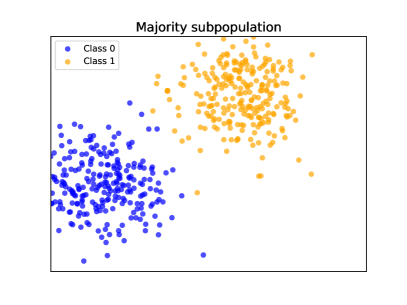
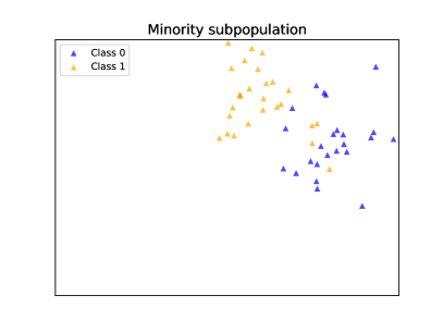
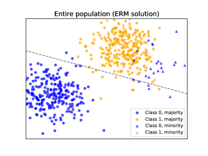
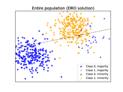
Majority: 97% correct, Minority: 58% correct	Majority: 83% correct, Minority: 82% correct

Figure 1: Illustration of the failings of Expected Risk Minimization (ERM) and i.i.d assumption in a linear binary classification problem, where the dataset can be partitioned to a majority and a minority subpopulation. ERM misclassifies a significant proportion of the minority subpopulation. DRO equalizes the performance across subpopulations. The DRO solution was obtained using the Lagrangian algorithm (Algorithm 1), both solutions use the same linear SVM model.

2 DRO versus data curation

Traditionally, training a model in machine learning seeks parameters, say, the weights $w$ of a neural networks, that minimize a risk $C_{P}(w)$ that is the expectation of a loss function with respect to a single distribution of training examples.

Alas, even when the training distribution is representative of the actual testing conditions, the trained system might perform very poorly on selected subsets of examples. For instance, Figure 1 describes a training problem where a majority population and a minority population have different classification boundaries. Minimizing the expected loss over the full dataset (bottom left plot) yields a system whose performance is skewed towards the majority population at the expense of the performance in the minority population. In real life, this can be a source of major injustice. Algorithms that optimize for minimum average error yield models that perform poorly on subpopulations that are already at risk due to pre-existing biases. This is most pronounced when ERM (based on minimising the average prediction error) produces solutions that privilege the majority populations over the minorities. This was shown to be consequential in scenarios such as court verdicts, loan applications, hiring and healthcare interventions (Datta et al., 2014; Chouldechova, 2017; Dastin, 2018; Rahmattalabi et al., 2019; Qian et al., 2020; Metz and Satariano, 2020; Angwin et al., 2020). For example, hiring systems and ad-targeting algorithms based on minimising average error were found to discriminate against female users by more frequently proposing executive and technical jobs to men (Datta et al., 2014; Dastin, 2018).

Distributionally Robust Optimization (DRO) seemingly addresses this problem by considering instead a collection $\mathcal{Q}$ of ‘training distributions’ and minimizing the expected risk observed on the most adverse distribution

$$\min_{w}~{}\max_{P\in\mathcal{Q}}C_{P}(w)~{}.$$ (1)

For instance, we can substantially reduce the performance differences reported in Figure 1 (bottom left plot). Using DRO with a set $\mathcal{Q}$ of two distributions, representing the majority and minority populations, leads to the decision boundary illustrated in Figure 1 (bottom right plot). This classifier does not reproduce the pre-existing imbalance between the majority and the minority subpopulation. Instead, the performance is equalized, and the average accuracy increases from $77.5\%$ to $82.5\%$.

As discussed more precisely in Section 3, the approach of using the basic definition of DRO (1) without additional information on the subpopulations is insufficient in practical applications. However, we argue that DRO remains an interesting building block because it provides a bridge between two common approaches to this problem, namely, ($i$) ensuring that the trained system has consistent performance across subpopulations, and ($ii$) curating the training set by remixing the populations until obtaining a more palatable result.

One of the contributions of our work is an ensemble of mathematical results that clarify the relation between finding a local minimum of the DRO problem (1) and (2) on one hand, and minimizing the usual expected risk with respect to a single, well crafted, training distribution. We hope these results will be useful for both the data-focused and the algorithm-focused sides of the bias debate in machine learning community.

For convex cost functions, these results are well known, because one can reformulate the DRO problem as a constrained optimization problem by introducing a slack variable $L$,

$$\min_{w,L}L~{}~{}~{}\text{s.t.}~{}~{}~{}\forall P\in\mathcal{Q}~{}C_{P}(w)\leq L~{},$$

and relying on standard convex duality results (Bertsekas, 2009) (see Section A.4. in the Appendix).

The point of our theoretical contribution is that similar results hold for the local minima of the nonconvex costs typical of modern deep learning systems, and also hold when the family $\mathcal{Q}$ is infinite. We now summarize the main results (the elaboration and proofs of these propositions are in the Appendix).

Let $\ell(z,w)$ be the loss of a machine learning model where $w\in\mathbb{R}^{d}$ represent the parameters of the model and $z\in\mathbb{R}^{n}$ belongs to the space of examples. For instance, in least square regression, the examples $z$ are pairs $(x,y)$ and the loss is $\ell(z,w)=\|y-f_{w}(x)\|^{2}$. When the collection $\mathcal{Q}$ is finite, under weak regularity assumptions, a DRO local minimum is always a stationary point of the expectation of the loss with respect to a suitable mixture of the DRO training distributions. Theorem 1 states this fact for a finite collection $\mathcal{Q}$ of distributions:

Theorem 1 (Finite case).

Let $\mathcal{Q}=\{P_{1},\dots,P_{K}\}$ be a finite set of probability distributions on $\mathbb{R}^{n}$ and let $w^{*}$ be a local minimum of the DRO problem (1) or the calibrated DRO problem (2). Let the costs $C_{P}(w)=\mathbb{E}_{z\sim P}[\ell(z,w)]$ be differentiable in $w^{*}$ for all $P\in\mathcal{Q}$. Then there exists a mixture distribution ${P_{\mathrm{mix}}}=\sum_{k}\lambda_{k}P_{k}$ such that $\nabla{C}_{{P_{\mathrm{mix}}}}(w^{*})=0$.

When the collection $\mathcal{Q}$ is infinite (possibly uncountably infinite) but satisfies a tightness condition (see Definition 1 in the Appendix), we can still show that a DRO local minimum is a stationary point for a well crafted training distribution. However, this training distribution is not necessarily a finite or countable mixture of the distributions found in $\mathcal{Q}$ but is always found in the weak closure of the convex hull of $\mathcal{Q}$. Adversarial robustness is an example of applying DRO on an infinite family of distributions (see a discussion of the implications of Theorem 2 in Section 5).

Theorem 2 (Infinite case).

Let $\mathcal{Q}$ be a tight family of probability distributions on $\mathbb{R}^{n}$. Let $w^{*}$ be a local minimum of problem (2). Let ${\mathcal{Q}_{\mathrm{mix}}}$ be the weak convergence closure of the convex hull of $\mathcal{Q}$. Let there be a bounded continuous function $h(z,w)$ defined on a neighborhood $\mathcal{V}$ of $w^{*}$ such that $\nabla{C}_{P}(w)=\mathbb{E}_{z\sim{P}}[h(z,w)]$ for all $P\in{\mathcal{Q}_{\mathrm{mix}}}$ and such that $\|h(z,w)-h(z,w^{\prime})\|\leq{M}\|w-w^{\prime}\|$ for almost all $z\in\mathbb{R}^{n}$. Then ${\mathcal{Q}_{\mathrm{mix}}}$ contains a distribution ${P_{\mathrm{mix}}}$ such that $\nabla_{w}C_{P_{\mathrm{mix}}}(w^{*})=0$.

Conversely, we consider a local minimum of the expectation of the loss with respect to an arbitrary mixture of distributions from $\mathcal{Q}$. Such a local minimum always is a local minimum of a calibrated DRO problem where one introduces suitable calibration constants $r_{P}$ that control how we compare the costs for different distributions:

$$\min_{w}~{}\max_{P\in\mathcal{Q}}~{}\left(C_{P}(w)-r_{P}\right)~{}.$$ (2)

We shall see in Section 3 that such calibration coefficients are in fact needed to express the subtleties of the original problem of learning from multiple subpopulations with DRO.

Theorem 3 (Converse).

Let ${P_{\mathrm{mix}}}=\sum_{k}\lambda_{k}P_{k}$ be an arbitrary mixture of distributions $P_{k}\in\mathcal{Q}$. If $w^{*}$ is a local minimum of $C_{P_{\mathrm{mix}}}$, then $w^{*}$ is a local minimum of the calibrated DRO problem (2) with calibration coefficients $r_{P}=C_{P}(w^{*})$.

Note that there is a discrepancy between these two theorems. Theorem 3 says that a local minimum of an expected risk mixture is a DRO local minimum, but Theorem 1 only says that a DRO local minimum is a stationary point (that is, a point with null derivative) of an expected risk mixture.

This distinction is moot when $\ell(z,w)$ are convex in $w$ because all stationary points are not only local minima, but also global minimum. When this is the case, Theorem 1 and Theorem 3 then describe the same equivalence as the standard convex duality results. In contrast, when the cost functions are nonconvex, the stationary point described in Theorem 1 need not even be a local minimum of the expected cost mixture. For instance, if the DRO local minimum is achieved in a region where all $C_{P}(w)$ have a negative curvature, then any mixture of these costs also has a negative curvature, and, as a result, the stationary point can only be a local maximum. Figure 2 shows how such a situation can arise in theory.

However, the learning algorithms that are typically used to train overparametrized deep learning models empirically follow trajectories where the Hessian is very flat apart from a few positive eigenvalues (Sagun et al., 2018). Weak negative curvature directions always exist —even when the algorithm stops making progress— but are very weak. In order to understand whether situations like Figure 2 happen in practice, it makes sense to now take a closer look at the algorithms commonly used to implement DRO.

Figure 2: Consider the two real functions $C_{1}(w)=\tanh(1+w)+\epsilon w^{2}$ and $C_{2}(w)=\tanh(1+w)+\epsilon w^{2}$. The minimum $w^{*}=0$ of $\max\{C_{1}(w),C_{2}(w)\}$ is a stationary point of the mixture cost $C_{\mathrm{mix}}(w)=\tfrac{1}{2}C_{1}(w)+\tfrac{1}{2}C_{2}(2)$. However, because it is achieved in negative curvature regions of $C_{1}$ and $C_{2}$, this stationary point is not a local minimum but a local maximum of the mixture cost. In practice, overparametrized deep learning models are unlikely to meet such a situation because the Hessian along the learning trajectories tend to be essentially flat apart from a few positive eigenvalues (Sagun et al., 2018).

In the convex case, it is known that increasing the weight of a distribution in the mixture is equivalent to reducing the corresponding calibration coefficient. This observation leads to a plethora of saddle-point seeking algorithms such as Uzawa iterations (Arrow et al., 1958). See Algorithm 1 for a representative example. Because such algorithms are reliable and can be made efficient, many authors advocate using similar strategies for nonconvex deep learning systems (e.g., (Sagawa et al., 2020)). Section A.4. in the Appendix shows how our theoretical results offer support for this practice. It also shows that such an algorithm fails to find DRO minima when the associated stationary point of the expected cost mixture is not itself a local minimum. For practical purposes, this means that there is no substantial difference between using such an efficient DRO algorithm and minimizing a well-crafted expected risk mixture.

Input: Equally sized training sets $D_{k}$ for $k=1\dots K$

Input: Calibration coefficients $r_{k}$. Initial weights $w_{0}$.

Input: Temperature $\beta$. Stopping threshold $\epsilon$.

Output: A sequence of weights $w_{t}$.

$t\leftarrow K$

$\lambda_{k}\leftarrow 1/t~{}~{}\forall k$

repeat

       $w_{t+1}\leftarrow\textnormal{{Descend}}\big{(}w_{t},\{D_{1}\star\lambda_{1}\dots D_{K}\star\lambda_{K}\}\big{)}$

       $c_{k}\leftarrow\textnormal{{Cost}}\big{(}w_{t+1},\{D_{k}\}\big{)}~{}~{}\forall k$

       $\delta_{k}\leftarrow\frac{1}{Z}\exp(\beta(c_{k}-r_{k}))~{}~{}\forall k$ — with $Z$ such that $\sum_{k}\delta_{k}=1$

       $\lambda_{k}\leftarrow\frac{1}{t+1}(t\lambda_{k}+\delta_{k})~{}~{}\forall k$

       $t\leftarrow t+1$

      

until $\max_{k}|\lambda_{k}-\delta_{k}|<t\epsilon$

return $w_{t}$

Algorithm 1 A typical Lagrangian DRO algorithm.

3 Calibration problems

As promised earlier, we now return to the statement of the simple DRO problem (1) and discuss how it fails to properly account for many subtleties of the bias fighting problem.

One set of issues is described in the algorithmic bias literature (Louizos et al., 2016; Beutel et al., 2017; Zhang et al., 2018; Hashimoto et al., 2018b; Amini et al., 2019). Representation disparity refers to the pheonomenon of achieving a high overall accuracy but low minority accuracy. For instance, ubiquitous speech recognition systems, such as voice assistants, struggle with accents and dialects (Behravan et al., 2016; Yang et al., 2018; Najafian and Russell, 2020). A minority user becomes discouraged by the poor performance of such system, which leads to disparity amplification over time due to the increasing gap between quantity of data provided by active users (majority groups, favored by the system from the beginning) and groups that experienced poor performance due to the initial representation disparity. This shows that it is sometimes justified to augment the DRO statement with means to favor certain subpopulations in order to account for representation disparity or disparity amplification. A related development is the method proposed by Sagawa et al. (Sagawa et al., 2020): in order to account for the potentially small size of the training data for some distributions $P$, they augment the cost $C_{P}(w)$ with a penalty that decreases when the number of training examples for this distribution increases.

There might also be instances where it is justifiable to account for the difference in difficulty across distributions. For instance, it might be known that one of the training distribution represents examples collected with a deficient method, such as, bad cameras, bad conditions, etc. Because the task is more difficult due to data limitations, the cost $C_{P}(w)$ for such a distribution will systematically be higher than for other distributions. The simple DRO formulation (1) then amounts to optimizing only for this distribution. As a consequence, small gains for the deficient distribution will be obtained at the expense of a massive performance degradation for all other distributions, essentially making it as bad as the performance for the deficient distribution. It might then be necessary to reduce the weight of this distribution in order to prevent it from dominating the DRO problem. In other words, the ideal solution to such a problem is to address the deficiencies of the data collection method.

Both issues (the need to account for pre-existing difficulties related to modelling certain subpopulations and the equalizing effect of DRO) can be addressed by augmenting the DRO problem with calibration constants that make such adjustments explicit. This leads to the calibrated DRO problem that we have already introduced when discussing Theorem 3 (Calibrated DRO 2). Specifying a set of calibration constants amounts to describing what we consider to be an acceptable outcome for the original bias fighting problem. What is acceptable or not is obviously problem dependent and can be the object of difficult controversies. Making the calibration constants explicit separates the mathematical optimization statement from the difficult task of deciding what results are acceptable in a real-world problem.

A consequence of the mathematical theory is the practical duality between calibration constants $r_{P}$ and mixture coefficients $\lambda_{P_{k}}$. Theorem 1 says that a DRO local minimum for a particular choice of calibration constants is a stationary point of the expected loss for a particular mixture of the original distributions. Conversely, Theorem 3 says that a local minimum of any particular expected risk mixture is also a DRO local minimum for a particular set of calibration constants.

The calibration constants $r_{P}$ might in fact be a better way than mixture coefficients $\lambda_{P_{k}}$ to specify which performance discrepancies are considered acceptable across subpopulations because there are useful reference points for choosing them. The first reference point is to use equal calibration constants. DRO then optimizes the performance of the most adverse subpopulation at the cost of potentially degrading the performance of the system for the remaining subpopulations. See Figure 1 for an example. Another approach is to use the calibration constants $r_{P}^{*}$ that represent the best performance we can reach with our machine learning model on each distribution $P$ in isolation.

$$r_{P}^{*}=\min_{w}C_{P}(w)$$

Solving the DRO problem for these calibration constants amounts to constructing a single machine learning system that performs almost as well on each distribution $P$ as a dedicated machine learning system specifically trained for distribution $P$ alone. In the following section, we elaborate on this method of setting calibration constants.

Note that based on Theorems 1 and 3, regardless of the chosen calibration constants, no DRO solution can achieve a performance better than $r_{P}^{*}$ on any distribution $P$. If this were the case, it would mean that $r_{P}^{*}$ was not correctly estimated, and the new performance would become the corrected $r_{P}^{*}$. This simple observation forms the basis for the practical recommendations discussed in the next section.

4 A minimal set of practical recommendations

In this section, we provide a minimal set of practical recommendations to machine learning engineers who face the difficult task of constructing and deploying bias-sensitive machine learning systems. We do not pretend that these recommendations are sufficient to address the bias problem, but merely represent intuitively sensible steps that are supported by our mathematical insights and should not be avoided. We summarize these recommendations in Inset 1.

We also motivate and elaborate on each step below.

1. Identify subpopulations $P_{k}$ at risk in the available data. 2. For each subpopulation, and in isolation, determine the best performance $r_{P_{k}}^{*}$ that can be achieved with the machine learning model of choice. 3. Decide whether the $r_{P_{k}}^{*}$ represent an acceptable set of performances. There is no point using DRO if this is not the case. Instead, investigate why the model performs so poorly on the adverse distributions (insufficient data, inadequate model, etc.) until obtaining an acceptable set of $r_{P_{k}}^{*}$. 4. Use DRO to construct a single machine learning system whose performance on each subpopulation is not much worse than $r_{P_{k}}^{*}$. This can be achieved by using the $r_{P_{k}}^{*}$ as calibration coefficients in a Lagrangian algorithm. 5. Deploy the system on an experimental basis in order to collect more data. Sample the examples with the lowest accuracy in order to determine whether we missed a subpopulation at risk. If one is found, add the vulnerable subpopulation to the initial data and repeat all the steps.

List of Insets 1 Summary of practical recommendations.

The identification of the subpopulations of concern frames the problem because it also defines the success criterion, that is, bias mitigation with respect to meaningful subpopulations. Key factors to consider are future users of the system, information on which groups have previously suffered from discrimination in similar scenarios, and the quantity and quality of the available data at the training time. In particular, we must at least have enough data to evaluate the subpopulation performances reliably. For instance, in a face recognition system, subpopulations might contain images of people representing distinct ethnicities (Klare et al., 2012).

Working on each subpopulation in isolation attempts to determine the best achievable performance on each subpopulation if this subpopulation were the only target. Data available for minority subpopulations might be limited. In such case, data from remaining subpopulations can be used as a regularizer to improve performance on the subpopulation $P$ of interest. For instance, we can train on a mixture of data coming from both the subpopulation $P$ (with weight $1$) and the remaining subpopulations (with weights $\alpha_{P}$). We then treat $\alpha_{P}$ as a hyperparameter that we tune to achieve the best validation performance on data from the subpopulation $P$. Our estimate of $r^{*}_{P}$ is then the performance of the resulting system, either measured on the validation set, or on held out data if such data is available in sufficient quantity. This is why it is important to have sufficient data to reliably validate a model performance on each subpopulation. Techniques proposed to tackle noisy datasets and scenarios with limited labelled examples (active learning (Ren et al., 2020), transfer learning (Pan and Yang, 2010; Tan et al., 2018)) can be used to increase the performance.

We can then judge whether the $r^{*}_{P}$ represent an acceptable set of performances for a final system. As explained in Section 3, no DRO solution can perform better on a subpopulation $P$ than a model trained for this subpopulation $P$ only. If the set of performances obtained in the previous steps is not acceptable, we must identify the root cause of this problem. For instance, if poor performance stems from insufficient data quality for the subpopulation, this problem will persist at the step of finding a consistent system using DRO. We need to then focus on improving data quality for vulnerable subpopulations. We recommend investigating the root cause of insufficient performance for each of the vulnerable subpopulations in isolation.

If minimum cost that can be achieved per each subpopulation is acceptable, we can then build a system that works consistently well across the subpopulations using DRO. In the simplest case, calibration coefficients $r_{P}$ per each subpopulation are going to be equal to the optimum expected risk for that subpopulation alone, $r_{P}=\min_{w}C_{P}(w)$. We can also adjust the calibration coefficients to prevent overfitting to individual subpopulations (Sagawa et al., 2020). For $n$ examples in a certain subpopulation $P$, the expected risk $C_{P}(w)$ can be replaced by its empirical estimate $C_{P_{n}}(w)+$ augmented with a calibration constant that decreases when the number $n$ of training examples increases. Moreover, the model size often needs to be larger than the model size that achieves the best performance on each individual subpopulations. Intuitively, this is needed because handling all subpopulations at once might be more demanding than handling only one. In Section 2 and Section A.4. in the Appendix, we also argue that overparametrization improves the issues associated with DRO local minima that are stationary points of an expected loss mixture but are not local minima of this mixture. As a result, overparametrization helps practical Lagragian DRO algorithms to find a good solution.

Finally, we must remain aware that the final system critically depends on the initial selection of the subpopulations of interest. Therefore, it remains essential to cautiously deploy such a system and to monitor its performance during the ramp up. In particular, the worst performing cases should be examined for consistent patterns that might indicate that a vulnerable subpopulation was not considered in the problem specification. When this is the case, the correct solution is to include the initially omitted subpopulation and start again.

5 DRO for adversarial examples

The previous sections make several observations about the application of DRO to fight bias in machine learning systems. In particular, we have argued that DRO is practically equivalent to training on a well chosen example distribution, and we have also shown that this well chosen example distribution is far from universal but depends on often implicit assumptions hidden in the DRO problem statement, such as calibration coefficients.

These observations extend beyond the bias fighting scenario. For instance, DRO is often presented as a good way to construct systems that are robust to adversarial examples (Szegedy et al., 2014; Madry et al., 2017). This application of DRO can be formalized by considering a set $\Phi$ of all measurable functions $\varphi$ that map an example pattern $z$ to another pattern $\varphi(z)$ that is assumed to be visually indistinguishable from $z$ according to a predefined criterion. For instance, it is common to consider the set of all transformations $\varphi$ such that $\|z-\varphi(z)\|_{p}\leq{\kappa}$, that is, transformations that can only modify an input pattern while remaining in a given $L_{p}$ ball.

Let $P_{\varphi}$ represent the distribution followed by $\varphi(z)$ when $z$ follows the distribution $P$. Robust solutions against the class of adversarial perturbation $\Phi$ can be expressed as the DRO problem

$$\min_{w}\left\{~{}~{}~{}\max_{\varphi\in\Phi}C_{P_{\varphi}}(w)~{}~{}=~{}~{}\max_{P_{\varphi}\in\mathcal{Q}}C_{P_{\varphi}}(w)~{}~{}~{}\right\}~{}.$$

The distribution family $\mathcal{Q}=\{P_{\varphi}:\varphi\in\Phi\}$ is typically much larger than the ones considered in the bias fighting scenario. Instead of representing a finite number of subpopulations, the family $\mathcal{Q}$ is usually infinite and uncountable. Therefore one cannot reduce this DRO problem to a finitely constrained optimization problem and one cannot use a separation lemma because the family $\mathcal{Q}$ or its convex hull may not be topologically closed.

Theorem 2 relies on an additional tightness assumption to establish that a DRO local minimum $w^{*}$ is also a stationary point of the expected risk for an example distribution that belongs to the weak closure of the convex hull of $\mathcal{Q}$. The tightness assumption is trivially satisfied when the examples belong to a bounded domain (as is the case for images) or when they remain close to reference images drawn from a single distribution (as is the case for adversarial examples).

At first sight, this result seems to imply that there is a distribution of images on which the ordinary training procedure yields a solution robust to adversarial examples. Is it true that we would not have adversarial example issues if only we had the right examples to start with? Or the right data augmentation scheme?

More precisely, Theorem 2 states that a DRO local minimum is a stationary point of the expected risk for an example distribution that depends on all the details of the DRO problem and in particular on the definition of the set $\Phi$ of adversarial perturbation, or equivalently on which images are considered visually indistinguishable from a reference image. On one hand, we could use DRO with a class of adversarial perturbations $\Phi$ that are very conservatively below the threshold of visual distinguishability. For instance, the perturbation might be limited to changing pixel values by no more than a small threshold. Alas, the solution might be fooled by adversarial examples that do not satisfy this strict condition but nevertheless are still visually indistinguishable from the original pattern. On the other hand, we could use DRO with much broader class of perturbation, potentially including some that would affect a human observer. For instance, dithering patterns might occasionally introduce enough noise to be perceptually meaningful. Because such perturbations can dominate the DRO problem, it becomes necessary to introduce calibration constants in order to account for the variation in performance that can be justifiably expected with such perturbations.

Because DRO is fundamentally related to minimizing the expected cost for a well crafted example distribution, DRO does not really solve the original problem but displaces it into the specification of the class of adversarial perturbations and the selection of the associated cost calibration constants. However, the adversarial example scenario is substantially more challenging than the bias fighting scenario: because the number of potential perturbations is much larger than the number of potentially vulnerable subpopulations, we cannot work around the problem by first working on each of them in isolation as suggested in Section 4. Using DRO for adversarial robustness without a reliable perceptual distance might be fundamentally flawed (Sharif et al., 2018).

6 Related work

Finding the appropriate choice for adversarial risk and making it match some notion of perceptual similarity is a topic of ongoing research. Early work on this topic considered $L_{p}$ norms as a similarity metric, for example $L_{0}$ (Papernot et al., 2015), $L_{2}$ (Szegedy et al., 2014), or $L_{\infty}$ (Goodfellow et al., 2014a). Sharif et al. (Sharif et al., 2018) show how these norms, as well as SSIM (Wang et al., 2004), fail to model perceptual similarity and still get fooled by simple adversarial examples. The view of adversarial machine learning through the lens of DRO is shared by Sinha et al. (Sinha et al., 2018), who use Wasserstein distance as a measure of perceptual similarity and achieve important statistical guarantees regarding the computed solution, as well as excellent practical performance.

Rahimian and Mehrotra (Rahimian and Mehrotra, 2019) survey recent research in DRO, and in particular mention the various ways risk can be defined. To the best of our knowledge, the question of what the calibration coefficients should be has not been the topic of much investigation. Meinshausen et al. (Meinshausen et al., 2015) propose setting $r_{P}=\operatorname{Var}[Y_{P}]$ in order to maximize the minimum explained variance across distributions. Our suggestion is based on accounting for the acceptable performance (the best obtainable performance in isolation) of a particular subpopulation.

One thread in the debate on the source of bias was inspired by the outcomes of applying a photo upsampling algorithm (Menon et al., 2020) to images of non-white people. Examples of using DRO to approach similar problems include text autocomplete tasks (Hashimoto et al., 2018a), noisy minority subpopulations (Wang et al., 2020) and protection with respect to specific sensitive attributes (Taskesen et al., 2020), as well as lexical similarity and recidivism prediction (Duchi et al., 2020). The phenomeonon of neural networks exploiting ’shortcuts’ in data (Geirhos et al., 2020) is a related line of work on robustness and fairness.

7 Conclusion

Whether fighting bias in machine learning systems is a data curation problem or an algorithmic problem has been the object of much discussion. Our theoretical results clarify the relation between a well known algorithmic approach, DRO, and the optimization of the expected cost on a well crafted data distribution. Contrary to the usual convex duality results, these results hold for nonconvex costs and for infinite families of distributions. These results also provide some support for the common practice of leveraging this quasi-equivalence to design efficient DRO algorithms. But it also becomes clear that running such an imperfect DRO algorithms is equivalent to optimizing the expected risk for a well crafted distribution.

This analysis also makes clear that this well crafted distribution is not universal but depends on often implicit details of the DRO problem setup such as calibration constants. Alas, in the same way that there is no universally robust training set, there is no universal way to define calibration constants that ensure an acceptable set of results. However, an elementary argument shows that one cannot reach acceptable results with DRO unless one can reach acceptable results on each subpopulation in isolation. This forms the basis for a minimal set of practical recommendations. Finally we discuss how our insights —this time with an infinite distribution family— raise concerns about the commonly advocated use of DRO to tame adversarial examples without a reliable perceptual similarity criterion.

Using DRO for fairness or adversarial robustness without a clear understanding of its algorithmic limitations can have a negative societal impact. Recommendations in Section 4 aim to prevent misuses of DRO, such as lowering performances on the remaining subpopulations to match the error on the most difficult distribution. However, as a consequence of Theorems 1, 2 and 3, it is also necessary to address the underlying problems in the most challenging distribution. On on hand, failure to address the issues in the minority subpopulation leaves it susceptible to discrimination, both in the application at hand and in the future applications, where the unresolved issues might persist. On the other hand, reducing the performance of the majority populations can lead to an unacceptable average performance, and as a result, the system is not going to be used — which might lead to a loss of interest in designing broadly accessible systems for this purpose (i.e., voice assistants robust to minority accents). We hope that our results and discussion will give more context to the debate on the sources of bias in machine learning, as well as help in bias mitigation in real-life scenarios.

Appendix A Theoretical Appendix

Notation

Let $\ell(z,w)$ be the loss of a machine learning model where $w\in\mathbb{R}^{d}$ represent the parameters of the model and $z\in\mathbb{R}^{n}$ belongs to the space of examples. For instance, in the case of least square regression, the examples $z$ are pairs $(x,y)$ and the loss is $\ell(z,w)=\|y-f_{w}(x)\|^{2}$.

Distribution Robust Optimization (DRO)

Instead of assuming the existence of a probability distribution $P(z)$ over the examples $z$ and formulating an Expected Risk Minimization (ERM) problem:

$$\min_{w}~{}~{}\left\{~{}C_{P}(w)=E_{z\sim{P}}[\ell(z,w)]~{}\right\},$$ (3)

the Distribution Robust Optimization (DRO) problem considers a family $\mathcal{Q}$ of distributions and seeks to minimize

$$\min_{w}~{}~{}\left\{\quad C_{\mathcal{Q}}(w)~{}\stackrel{{\scriptstyle\Delta}}{{=}}~{}\max_{P\in\mathcal{Q}}C_{P}(w)~{}=~{}\max_{P\in\mathcal{Q}}E_{z\sim{P}}[\ell(z,w)]\quad\right\}.$$ (4)

Many authors define $\mathcal{Q}$ with the purpose of constructing a learning algorithm with additional robustness properties. For instance, $\mathcal{Q}$ may be the set of all distributions located within a certain distance of the training distribution [Bagnell, 2005, Namkoong and Duchi, 2016, Blanchet et al., 2019, Staib and Jegelka, 2019]. Different ways to measure this distance lead to different and sometimes surprising solutions [e.g., Hu et al., 2018]. Interesting theoretical possibilities appear when $\mathcal{Q}$ also contains the discrete distributions that represent finite training sets. Besides these theoretically justified choices of $\mathcal{Q}$, many practical concerns can be viewed through the prism of DRO on ad-hoc families $\mathcal{Q}$ of distributions.

Example 1 (Fighting bias).

Let the example distributions $P_{1}$ to $P_{K}$ represent identified subpopulations for which we want to ensure consistent performance. It is appealing to formulate this problem as a DRO problem with $\mathcal{Q}=\{P_{1}\dots P_{K}\}$. However, as discussed in the main text, it is important to realize that much of the original problem is hiding behind the choice of the calibration constants.

Example 2 (Fighting adversarial attacks).

Szegedy et al. [2014] have shown that one can almost arbitrarily change the output of a deep learning vision system by modifying the patterns in nearly invisible ways. Let $\Phi$ be the set of all measurable functions $\varphi$ that map an example pattern $z$ to another pattern $\varphi(z)$ that is assumed visually indistinguishable from $z$ according to a certain psycho-visual criterion. Let $P_{\varphi}$ represent the distribution followed by $\varphi(z)$ when $z$ follows the distribution $P$. Robust solutions against the class of adversarial perturbation $\Phi$ can be found with DRO with the distribution family $\mathcal{Q}=\{P_{\varphi}:\varphi\in\Phi\}$.

Calibrated costs

The simple DRO formulation makes sense when we know that all distributions define problems of comparable difficulty. It is however easy to imagine that a particular distribution emphasises harder examples. We can introduce calibration terms $r_{P}$ in the DRO formulation to prevent any single distribution $P$ to dominate the maximum.

$$\min_{w}~{}~{}\left\{\quad C_{\mathcal{Q},r}(w)~{}\stackrel{{\scriptstyle\Delta}}{{=}}~{}\max_{P\in\mathcal{Q}}\{C_{P}(w)-r_{P}\}\quad\right\}.$$ (5)

Correctly setting the calibration terms is both difficult and application specific. A simple but costly approach consists in letting $r_{P}$ be equal to the optimum cost for that distribution alone, $r_{P}=\min_{w}C_{P}(w)$. Calibrated DRO (5) then controls the loss of performance incurred by seeking a solution that works for all distributions as opposed to solutions that are specific to each distribution. Another approach [Meinshausen and Bühlmann, 2015] relies instead on the variance of the predicted quantity.

Calibration terms can also be used to counter the effect of finite training data. For instance, when we only have $n$ examples for a certain distribution $P\in\mathcal{Q}$, the expected risk $C_{P}(w)$ can be replaced by its empirical estimate $C_{P_{n}}(w)+$ augmented with a calibration constant that decreases when the number $n$ of training examples increases [Sagawa et al., 2020].

A.1 A local minimum of a DRO problem is a stationary point of an expected loss mixture

A.1.1 Finite case

We first address the case where $\mathcal{Q}$ is a finite set of distributions $P_{1}\dots P_{K}$. The following result simplifies Proposition 2 of Arjovsky et al. [2019] by eliminating the KKT constraint qualification requirement. In the rest of this document, we always assume that the mixture coefficients $\lambda_{k}$ are nonnegative and sum to one.

Theorem 1.

Let $\mathcal{Q}=\{P_{1},\dots,P_{K}\}$ be a finite set of probability distributions on $\mathbb{R}^{n}$ and let $w^{*}$ be a local minimum of the DRO problem (4) or the calibrated DRO problem (5). Let the costs $C_{P}(w)=\mathbb{E}_{z\sim P}[\ell(z,w)]$ be differentiable in $w$ for all $P\in\mathcal{Q}$. Then there exists a mixture distribution ${P_{\mathrm{mix}}}=\sum_{k}\lambda_{k}P_{k}$ such that $\nabla{C}_{{P_{\mathrm{mix}}}}(w^{*})=0$.

The proof relies on a simple hyperplane separation lemma closely related to Farkas’ lemma [Boyd and Vandenberghe, 2014, Sec.2.5 and Ex.2.20].

Lemma 1.

A nonempty closed convex subset $A$ of $\mathbb{R}^{n}$ either contains the origin or is strictly separated from the origin by a certain hyperplane, that is, there exists a vector $u\in\mathbb{R}^{n}$ and a scalar $c>0$ such that, for all $x\in{A}$, $\left<{u},{x}\right>\geq{c}$.

Proof.

Assume $0\notin{A}$. Let $u\in{A}$ be the projection of the origin onto the closed convex set $A$. For all $x\in{A}$ and all $t\in[0,1]$, the point $u+t(x-u)$ also belongs to the convex set $A$. Since $u$ is the point of $A$ closest to the origin,

$$\forall t\in[0,1]~{}~{}r(t)=\|u+t(x-u)\|^{2}=\|u\|^{2}+2t\left<{u},{x-u}\right>+t^{2}\|x-u\|^{2}\geq\|u|^{2}.$$

Therefore $r^{\prime}(0)=2\left<{u},{x-u}\right>\geq 0$, that is, $\left<{u},{x}\right>\geq\left<{u},{u}\right>>0$. ∎

Proof of Theorem 1.

Let $A\subset\mathbb{R}^{n}$ be the convex hull of the $g_{k}{=}\nabla{C}_{P_{k}}(w^{*})$ for $k=1\dots K$. $A$ is closed and convex. If $A$ does not contain the origin, according to the lemma, there exist $u$ and $c$ such that $\forall~{}x\in{A}$, $\left<{u},{x}\right>\geq{c}>0$. Therefore, for all $t>0$, moving from $w^{*}$ to $w^{*}-tu$ reduces all costs $C_{P_{k}}$ by at least $tc+o(t)$. As a consequence, $\max_{k}C_{P_{k}}$ is also reduced by at least $tc+o(t)$, contradicting the assumption that $w^{*}$ is a local minimum. Hence $A$ contains the origin, which means that there are positive mixture coefficients $\lambda_{k}$ summing to one such that $\sum_{k}\lambda_{k}\nabla{C}_{P_{k}}(w)=\nabla_{w}C_{P_{\mathrm{mix}}}(w)=0.$ ∎

All local and global solutions of the DRO problem (4) or (5) are therefore stationary points of the expected risk (3) associated with a mixture of the distributions of $\mathcal{Q}$. The exact mixture coefficients depend on the loss functions, the distributions included in $\mathcal{Q}$ and, in the case of the calibrated version of DRO, on the calibration constants $r_{P}$.

This result raises several important questions. Is this result valid when $\mathcal{Q}$ is not finite? Are these stationary points always local minima? Is the converse true? What is the relation between the mixture coefficients $\lambda_{k}$ and the calibration constants $r_{P}$? How far can such results go without assuming convex losses? These questions will be addressed in the rest of this document.

A.1.2 Infinite case

The infinite case differs because the convex hull of an infinite set of vectors is not necessarily closed, even when the original set is closed. Therefore cannot directly apply the lemma to the convex hull $A$ of the gradients $g_{P}=\nabla{C}_{P}(w^{*})$ for all $P\in\mathcal{Q}$. Appling instead the lemma to the closure $\bar{A}$ of $A$ yields a substantially weaker result: if $w^{*}$ is a local DRO minimum, then for each $\varepsilon>0$, there is a mixture ${{P_{\mathrm{mix}}^{(\varepsilon)}}}$ of distributions from $\mathcal{Q}$ such that $\|\nabla{C}_{\smash{{P_{\mathrm{mix}}^{(\varepsilon)}}}}\|\leq\varepsilon$.

Note there is no guarantee that ${{P_{\mathrm{mix}}^{(\varepsilon)}}}$ converges to an actual distribution when $\varepsilon$ converges to zero. Therefore this weaker result does not help relating the solution of a DRO problem with the solutions of an ERM problem for a suitable training distribution. However such a stronger result can be obtained at the price of a tightness assumption [Billingsley, 1999].

Definition 1.

A family of distributions $\mathcal{Q}$ on a Polish space $\Omega$ is tight when, for any $\epsilon>0$, there is a compact subset $K\subset\Omega$ such that $\forall P\in\mathcal{Q}$, $P(K)\geq 1-\epsilon$.

Tightness is therefore obvious when all the examples belong to a bounded domain. Even when this is not the case, it is known that any finite set of probability distributions on a Polish space is tight [Billingsley, 1999]. This often provides the means to prove the tightness of an infinite family $\mathcal{Q}$ of distributions that are "close" enough to a single distribution such as the training data distribution. For instance, in the case of adversarial examples (Example 2), tightness is doubly obvious, first because all images belong to a bounded domain, second because the visual similarity criterion ensures that the distance between $z$ and $\varphi(z)$ is bounded.

Theorem 2.

Let $\mathcal{Q}$ be a tight family of probability distributions on $\mathbb{R}^{n}$. Let $w^{*}$ be a local minimum of problem (5). Let ${\mathcal{Q}_{\mathrm{mix}}}$ be the weak convergence closure of the convex hull of $\mathcal{Q}$. Let there be a bounded continuous function $h(z,w)$ defined on a neighborhood $\mathcal{V}$ of $w^{*}$ such that $\nabla{C}_{P}(w)=\mathbb{E}_{z\sim{P}}[h(z,w)]$ for all $P\in{\mathcal{Q}_{\mathrm{mix}}}$ and such that $\|h(z,w)-h(z,w^{\prime})\|\leq{M}\|w-w^{\prime}\|$ for almost all $z\in\mathbb{R}^{n}$. Then ${\mathcal{Q}_{\mathrm{mix}}}$ contains a distribution ${P_{\mathrm{mix}}}$ such that $\nabla_{w}C_{P_{\mathrm{mix}}}(w^{*})=0$.

Following Bottou et al. [2018], the theorem does not require the loss $\ell(z,w)$ to be differentiable everywhere as long as the purported derivative $h(z,w)$ has the correct expectation. For our purposes, it must also be bounded and continuous on $\mathcal{V}$ and satisfy a Lipschitz continuity requirement.

Proof.

Let $\bar{A}$ be the closure of the convex hull of the $g_{P}=\nabla C_{P}(w^{*})$ for all $P\in\mathcal{Q}$. According to Lemma 1, if $\bar{A}$ does not contain the origin, then there are $u$ and $c>0$ such that $\forall x\in{A},\left<{u},{x}\right>>c$. In particular, for all $P\in\mathcal{Q}$, we have $\left<{u},{\nabla{C_{P}}(w^{*})}\right>>c>0$. Thanks to the Lipschitz continuity of $h(z,w)$, we have $C_{P}(w^{*}-tu)<C_{P}(w^{*})-tc+Mt^{2}$ for all $P\in\mathcal{Q}$. Therefore for any $0<t<c/2M$ and any $P\in\mathcal{Q}$, we have $C_{P}(w^{*}-tu)<C_{P}(w^{*})-tc/2$ contradicting the assumption that $w^{*}$ is a local DRO miminum. Therefore $\bar{A}$ contains the origin. This means that for any $t>0$, there exists a mixture ${P_{\mathrm{mix}}^{(1/t)}}$ of distributions from $\mathcal{Q}$ such that $\|\nabla{C_{\smash{{P_{\mathrm{mix}}^{(\varepsilon)}}}}}(w^{*})\|<1/t$. Note that if $\mathcal{Q}$ is tight, the convex hull of $\mathcal{Q}$ is also tight. Therefore the sequence ${P_{\mathrm{mix}}^{(1/t)}}$ is also tight, and, by Prokhorov’s theorem, contains a weakly convergent subsequence whose limit ${P_{\mathrm{mix}}}$ belongs to the closure ${\mathcal{Q}_{\mathrm{mix}}}$ of the convex hull of $\mathcal{Q}$. Because $h(z,w^{*})$ is continuous and bounded, the map $P\mapsto\nabla{C_{P}}(w^{*})$ is continuous for the weak topology. Therefore $\nabla{C_{P_{\mathrm{mix}}}})(w^{*})=0$. ∎

A.2 A local minimum of an expected loss mixture is a local minimum of a calibrated DRO problem

The following elementary result states that if $w^{*}$ is a local minimum of an expected cost mixture $C_{P_{\mathrm{mix}}}$, then it also is a local minimum of the calibrated DRO problem (5) with calibration constants $r_{P}$ equal to the costs $C_{P}(w^{*})$.

Theorem 1 (Converse).

Let ${P_{\mathrm{mix}}}=\sum_{k}\lambda_{k}P_{k}$ be an arbitrary mixture of distributions $P_{k}\in\mathcal{Q}$. If $w^{*}$ is a local minimum of $C_{P_{\mathrm{mix}}}$, then $w^{*}$ is a local minimum of the calibrated DRO problem (5) with calibration coefficients $r_{P}=C_{P}(w^{*})$.

Proof.

By contradiction, assume that $w^{*}$ is not a local minimum of (5), that is, for all $\epsilon>0$ there exists $u$ such that $\|u\|<\epsilon$ and $\max_{P\in\mathcal{Q}}\left\{C_{P}(w^{*}+u)-r_{P}\right\}<\max_{P\in\mathcal{Q}}\left\{C_{P}(w^{*})-r_{P}\right\}$. Recalling our choice of $r_{P}$ yields $\max_{P\in\mathcal{Q}}\left\{C_{P}(w^{*}+u)-C_{P}(w^{*})\right\}<0$. Since $C_{P}(w*+u)<C_{P}(w^{*})$ for all $P\in\mathcal{Q}$, $C_{P_{\mathrm{mix}}}(w^{*}+u)<C_{P_{\mathrm{mix}}}(w^{*})$, and $w^{*}$ cannot be a local minimum of $C_{P_{\mathrm{mix}}}$. ∎

A.3 With and without convexity assumptions

Note that there is a discrepancy between the statements of Theorem 3 and Theorems 1-2. The former requires a local minimum of the expected loss mixture, whereas the latter only provides a stationary point. This distinction becomes moot if we assume that the loss functions $\ell(z,w)$ are convex in $w$. When this is the case, all stationary points are not only local minima, but global minima as well. Theorems 1 and theorem 3 then provide an exact equivalence between finding a minimum of the calibrated DRO problem (5) and finding a minimum of an expected loss mixture.

However there is little point in providing theorems for the convex case because, at least in the finite case, it is well covered by theory of convex duality [Bertsekas, 2009] applied to a simple restatement of convex DRO as a convex optimization problem with an additional slack variable $L$

$$\min_{w,L}L\quad\text{s.t.}\quad\forall P\in\mathcal{Q}~{}~{}C_{P}(w)-r_{P}-L\leq 0~{}.$$

Convex duality also clarifies the relation between the mixture coefficients $\lambda_{k}$ and the calibration constants  $r_{P_{k}}$. Increasing the weight of a distribution in the mixture is equivalent to reducing the corresponding calibration coefficient. This observation then leads to a plethora of saddle-point seeking algorithms such as Uzawa iterations [Arrow et al., 1958] (see Section A.4.).

Figure 3: The minimum $w^{*}=0$ of $\max\{C_{1}(w),C_{2}(w)\}$ is a stationary point of the mixture cost $C_{\mathrm{mix}}(w)=\tfrac{1}{2}C_{1}(w)+\tfrac{1}{2}C_{2}(2)$. However this stationary point is not a local minimum but a local maximum of the mixture cost.

The nonconvex case is more challenging because the stationary points identified by Theorem 1 need not be local minima. Consider for instance the two real functions

$$C_{1}(w)=\tanh(1+w)+\epsilon w^{2}~{}~{}\text{and}~{}~{}C_{2}(w)=\tanh(1-w)+\epsilon w^{2}$$

where the term $\epsilon w^{2}$ with $0<\epsilon\ll 1$ is only present to ensure that each of these functions has a well defined optimum. As shown in Figure 3, their maximum $\max\{C_{1}(w),C_{2}(w)\}$ has a a minimum in $w^{*}=0$. As predicted by Theorem 1, this solution is a stationary point of the the mixture $C_{\mathrm{mix}}=\tfrac{1}{2}C_{1}(w)+\tfrac{1}{2}C_{2}(w)$. However this stationary point is not a local minimum but a local maximum.

This situation is in fact easy to understand. The solution $w^{*}{=}0$ of the problem $\min_{w}\max\{C_{1}(w),C_{2}(w)\}$ (Figure 3) falls in negative curvature regions of the functions $C_{1}$ and $C_{2}$. As a result any mixture of these two costs also has negative curvature in $w^{*}$. Therefore, the stationary point $w^{*}$ cannot be a local minimum. It is also easy to see that this situation cannot occur when the optimum of the DRO problem is achieved in points where the individual cost functions have positive curvature. Since all mixtures must also have positive curvature on these points, the stationary points can only be local minima. This remark is important because learning algorithms for deep learning problems tend to follow trajectories where the Hessian is very flat apart from a few positive eigenvalues [Sagun et al., 2018]. Weak negative curvature directions always exist —even when the algorithm stops making progress— but are very weak. Although we lack a good understanding of these landscapes, it seems a safe bet to assume that the situation presented in Figure 3 is often cured by overparametrization. The following section reaches a similar conclusion with closer look at a popular family of DRO algorithms.

A.4 Lagrangian algorithms for DRO

The calibrated DRO problem (5) is easily rewritten as a constrained optimization problem by introducing a slack variable $L$:

$$\min_{w,L}L\quad\text{s.t.}\quad\forall P\in\mathcal{Q}.~{}~{}~{}~{}C_{P}(w)-r_{P}-L\leq 0~{}.$$

With convex loss function, finite $\mathcal{Q}$, and under adequate qualification conditions [Boyd and Vandenberghe, 2014, Bertsekas, 2009], convex duality theory suggests to write the Lagrangian

$$L(w,M,\lambda_{1}\dots\lambda_{K})=M+\sum_{k}\lambda_{k}\big{(}C_{P_{k}}(w)-r_{P}-M\big{)}~{},$$

and solve instead the dual problem,

$$\max_{\lambda_{k}\geq 0}~{}\left\{D(\lambda_{1}\dots\lambda_{K})\stackrel{{\scriptstyle\Delta}}{{=}}\min_{w,M}L(w,M,\lambda_{1}\dots\lambda_{K})\right\}$$

The solution of this problem must satisfy $\sum_{k}\lambda_{k}=1$ because the dual $D(\lambda_{1}\dots\lambda_{k})$ is $-\infty$ when this is not the case. With this knowledge, the dual problem becomes

$$\max_{\begin{array}[]{c}\scriptstyle\lambda_{k}\geq 0\\[-2.41112pt] \scriptstyle\sum_{k}\!\lambda_{k}=1\end{array}}\left\{D(\lambda_{1}\dots\lambda_{K})=\left(\min_{w}\sum_{k}\lambda_{k}C_{P_{k}}(w)\right)-\left(\sum_{k}\lambda_{k}r_{P_{k}}\right)\right\}~{}.$$

The inner optimization problem is precisely the minimization of the expected risk with respect to the mixture $\sum_{k}\lambda_{k}P_{k}$ and therefore lends itself to many popular gradient descent methods. The mixture coefficients $\lambda_{k}$ must then be slowly adjusted by ascending the outer optimization objective [Arrow et al., 1958].

Input: Equally sized training sets $D_{k}$ for $k=1\dots K$

Input: Calibration coefficients $r_{k}$. Initial weights $w_{0}$.

Input: Temperature $\beta$. Stopping threshold $\epsilon$.

Output: A sequence of weights $w_{t}$.

$t\leftarrow K$

$\lambda_{k}\leftarrow 1/t~{}~{}\forall k$

repeat

       $w_{t+1}\leftarrow\textnormal{{Descend}}\big{(}w_{t},\{D_{1}\star\lambda_{1}\dots D_{K}\star\lambda_{K}\}\big{)}$

       $c_{k}\leftarrow\textnormal{{Cost}}\big{(}w_{t+1},\{D_{k}\}\big{)}~{}~{}\forall k$

       $\delta_{k}\leftarrow\frac{1}{Z}\exp(\beta(c_{k}-r_{k}))~{}~{}\forall k$ — with $Z$ such that $\sum_{k}\delta_{k}=1$

       $\lambda_{k}\leftarrow\frac{1}{t+1}(t\lambda_{k}+\delta_{k})~{}~{}\forall k$

       $t\leftarrow t+1$

      

until $\max_{k}|\lambda_{k}-\delta_{k}|<t\epsilon$

return $w_{t}$

Algorithm 2 A typical Lagrangian DRO algorithm.

Algorithm 2 is a typical example of this strategy. Although this particular instance uses a temperature parameter $\beta$ to smooth the mixture coefficient update rule, it is also common to focus on a single term with $\beta=+\infty$. When this is the case, each outer iteration of Algorithm 2 merely amounts to augmenting the training set with an extra copy of the examples associated with most adverse subpopulation.

Because of their simplicity and effectiveness, such Lagrangian DRO algorithms are widely used with deep learning system with nonconvex objectives [Sagawa et al., 2020, Augustin et al., 2020]. The theoretical results discussed in this appendix provide a measure support for this practice.

A crucial assumption for this algorithm is the idea that increasing the weight of a distribution in the mixture amounts to finding a local DRO minimum with a lower calibration coefficient for that distribution. This is true in the convex case. This requires a more precise discussion in the nonconvex case. Suppose for instance that one modifies the mixture coefficients by slightly increasing $\lambda_{1}$ by a small $\delta>0$ and re-normalizing:

$$\lambda^{\prime}_{1}=\tfrac{1}{Z}(\lambda_{1}+\delta)\qquad\lambda^{\prime}_{k}=\tfrac{1}{Z}\lambda_{k}~{}~{}\forall k>1$$

Such a change can yield two outcomes. Either $w^{*}$ remains a local minimum of the new expected cost mixture, or we can follow a descent trajectory and reach a new local minimum $w^{\prime}$:

$$Z\sum_{k}\lambda^{\prime}_{k}C_{P_{k}}(w^{\prime})~{}<~{}Z\sum_{k}\lambda^{\prime}_{k}C_{P_{k}}(w^{*})~{}.$$ (6)

• Let us first assume that the old cost function increases when one moves from its local minimum $w^{*}$ to the local minimum $w^{\prime}$ of the new cost function

  $$\sum_{k}\lambda_{k}C_{P_{k}}(w^{\prime})~{}\geq~{}\sum_{k}\lambda_{k}C_{P_{k}}(w^{*})$$ (7)

  Subtracting (7) from (6) yields

  $$\delta C_{P_{1}}(w^{\prime})<\delta C_{P_{1}}(w^{*})~{},$$

  which, according to Theorem 3, means that the new local minimum $w^{\prime}$ is a local minimum of a DRO problem with a reduced calibration coefficient for distribution $P_{1}$, just as for convex losses.

• However, it is also conceivable that (7) does not hold. This means that the new minimum $w^{\prime}$ achieves a lower cost than $w^{*}$ for both the old and new mixture costs. In other words, tweaking the mixture allowed us to escape the attraction basin of the local minimum $w^{*}$. From the perspective of algorithm 2, this disrupts the determination of the mixture coefficient, but this is nevertheless progress because both the old and new mixture costs are lower. In theory, this can only happen a finite number of times in a neural network because there is only a finite number of attraction basins. In practice, this never happens: stochastic gradient descent in neural networks usually follows a path with slowly decreasing cost without hopping from one attraction basin to another one [Goodfellow et al., 2014b, Sagun et al., 2018].

As mentioned earlier, it is also conceivable that $w^{*}$ remains a local minimum with the new mixture cost. Algorithm 2 then keeps increasing the weight of distribution $P_{1}$ as longs as the cost $C_{P_{1}}(w^{*})=C_{P_{1}}(w^{\prime})$ remains too high with respect to the desired calibration coefficients. This last case covers two distinct scenarios.

• The Lagrangian algorithm could keep increasing the weight of the first distribution without moving away from the local minimum $w^{*}$. The inner loop eventually minimizes the empirical risk for the first distribution only, yet without achieving progress. This suggests that we have reached a disappointing bound on the best performance achievable with our model using training data sampled from this first distribution.

• Alternatively, the old mixture local minimum $w^{*}$ could stop being a local minimum of the new mixture once the first distribution weight reaches a certain threshold. Consider for instance the problem of Figure 3. Even though the DRO minimum corresponds to a local maximum of the mixture cost $C_{\mathrm{mix}}(w)=\tfrac{1}{2}C_{1}+\tfrac{1}{2}C_{2}$, Theorem 3 tells us that both minima of this mixture cost are also local DRO minima, albeit for different calibration constants $r_{i}$. Figure 5 shows the case where $r_{2}>r_{1}$. Figure 5 shows that increasing the weight of the second cost function beyond a certain threshold eventually erases the left minimum and causes Algorithm 2 to jump to the condition $r_{1}>r_{2}$. In other words, our algorithm is not able to simultaneously keep both cost functions as low as they could separately be. This either suggests that these two goals are incompatible, or that the model does not have enough capacity to simultaneously achieve them together. As usual with neural networks, the remedy is overparametrization…

Figure 4: Both minima of $C_{\mathrm{mix}}(w)=\tfrac{1}{2}C_{1}+\tfrac{1}{2}C_{2}$ are solutions of a DRO problem, albeit one with different calibration constants $r_{1}$ and $r_{2}$. Here $r_{2}>r_{1}$.

Figure 5: Increasing the weight of the second distribution beyond a certain threshold erases the first minimum and causes Algorithm 2 to jump to the other minimum which is a calibrated DRO minimum for $r_{1}>r_{2}$.

One can derive two conclusions from this brief analysis. First, as long as we use a Lagrangian descent algorithm to solve the DRO problem, there is little point being concerned about stationary points of the mixture cost that are not local minima because (1) the algorithm is not going to find them anyway, and (2) overparametrizing the network is likely to make them disappear anyway (scenario $iv$ above). Second, the most concerning scenario is the case where a single distribution or subpopulation dominates the DRO problem because our model is unable to achieve a satisfactory performance even when it is trained to minimize the expected cost for that distribution only. When this is the case, DRO cannot help.

References

- Amini et al. [2019] Alexander Amini, Ava P. Soleimany, Wilko Schwarting, Sangeeta N. Bhatia, and Daniela Rus. Uncovering and Mitigating Algorithmic Bias through Learned Latent Structure. In Vincent Conitzer, Gillian K. Hadfield, and Shannon Vallor, editors, Proceedings of the 2019 AAAI/ACM Conference on AI, Ethics, and Society, AIES 2019, Honolulu, HI, USA, January 27-28, 2019, pages 289–295. ACM, 2019. doi: 10.1145/3306618.3314243. URL https://doi.org/10.1145/3306618.3314243.
- Angwin et al. [2020] Julia Angwin, Jeff Larson, Surya Mattu, and Lauren Kirchner. Machine bias: There’s software used across the country to predict future criminals. And it’s biased against blacks. ProPublica, 2020.
- Arjovsky et al. [2019] Martin Arjovsky, Léon Bottou, Ishaan Gulrajani, and David Lopez-Paz. Invariant Risk Minimization. arXiv CoRR, abs/1907.02893, 2019. URL http://arxiv.org/abs/1907.02893.
- Arrow et al. [1958] K Arrow, L. Hurwicz, and H. Uzawa. Studies in Nonlinear Programming. Stanford Univ. Press, 1958.
- Augustin et al. [2020] Maximilian Augustin, Alexander Meinke, and Matthias Hein. Adversarial robustness on in-and out-distribution improves explainability. In European Conference on Computer Vision, pages 228–245. Springer, 2020.
- Bagnell [2005] J. Andrew Bagnell. Robust Supervised Learning. In Manuela M. Veloso and Subbarao Kambhampati, editors, Proceedings, The Twentieth National Conference on Artificial Intelligence and the Seventeenth Innovative Applications of Artificial Intelligence Conference, July 9-13, 2005, Pittsburgh, Pennsylvania, USA, pages 714–719. AAAI Press / The MIT Press, 2005.
- Behravan et al. [2016] Hamid Behravan, Ville Hautamäki, Sabato Marco Siniscalchi, Tomi Kinnunen, and Chin-Hui Lee. i-Vector Modeling of Speech Attributes for Automatic Foreign Accent Recognition. IEEE ACM Trans. Audio Speech Lang. Process., 24(1):29–41, 2016. doi: 10.1109/TASLP.2015.2489558. URL https://doi.org/10.1109/TASLP.2015.2489558.
- Ben-Tal et al. [2009] Aharon Ben-Tal, Laurent El Ghaoui, and Arkadi Nemirovski. Robust Optimization, volume 28 of Princeton Series in Applied Mathematics. Princeton University Press, 2009. ISBN 978-1-4008-3105-0. doi: 10.1515/9781400831050. URL https://doi.org/10.1515/9781400831050.
- Bertsekas [2009] D.P. Bertsekas. Convex Optimization Theory. Athena Scientific optimization and computation series. Athena Scientific, 2009.
- Beutel et al. [2017] Alex Beutel, Jilin Chen, Zhe Zhao, and Ed H. Chi. Data Decisions and Theoretical Implications when Adversarially Learning Fair Representations. CoRR, abs/1707.00075, 2017. URL http://arxiv.org/abs/1707.00075.
- Billingsley [1999] Patrick Billingsley. Convergence of probability measures. Wiley Series in Probability and Statistics: Probability and Statistics. John Wiley & Sons Inc., New York, 1999. ISBN 0-471-19745-9.
- Blanchet et al. [2019] Jose Blanchet, Yang Kang, and Karthyek Murthy. Robust Wasserstein profile inference and applications to machine learning. Journal of Applied Probability, 56(3):830–857, 2019.
- Bottou et al. [2018] Léon Bottou, Frank E. Curtis, and Jorge Nocedal. Optimization Methods for Large-Scale Machine Learning. Siam Reviews, 60(2):223–311, 2018.
- Boyd and Vandenberghe [2014] Stephen P. Boyd and Lieven Vandenberghe. Convex Optimization. Cambridge University Press, 2014.
- Chouldechova [2017] Alexandra Chouldechova. Fair Prediction with Disparate Impact: A Study of Bias in Recidivism Prediction Instruments. Big Data, 5(2):153–163, 2017. doi: 10.1089/big.2016.0047. URL https://doi.org/10.1089/big.2016.0047.
- Dastin [2018] Jeffrey Dastin. Amazon scraps secret AI recruiting tool that showed bias against women. Reuters, 2018.
- Datta et al. [2014] Amit Datta, Michael Carl Tschantz, and Anupam Datta. Automated Experiments on Ad Privacy Settings: A Tale of Opacity, Choice, and Discrimination. CoRR, abs/1408.6491, 2014. URL http://arxiv.org/abs/1408.6491.
- Derman and Mannor [2020] Esther Derman and Shie Mannor. Distributional robustness and regularization in reinforcement learning. arXiv preprint arXiv:2003.02894, 2020.
- Duchi et al. [2020] John Duchi, Tatsunori Hashimoto, and Hongseok Namkoong. Distributionally robust losses for latent covariate mixtures. arXiv preprint arXiv:2007.13982, 2020.
- Geirhos et al. [2020] Robert Geirhos, Jörn-Henrik Jacobsen, Claudio Michaelis, Richard S. Zemel, Wieland Brendel, Matthias Bethge, and Felix A. Wichmann. Shortcut Learning in Deep Neural Networks. CoRR, abs/2004.07780, 2020. URL https://arxiv.org/abs/2004.07780.
- Goodfellow et al. [2014a] Ian J Goodfellow, Jonathon Shlens, and Christian Szegedy. Explaining and harnessing adversarial examples. arXiv preprint arXiv:1412.6572, 2014a.
- Goodfellow et al. [2014b] Ian J Goodfellow, Oriol Vinyals, and Andrew M Saxe. Qualitatively characterizing neural network optimization problems. arXiv preprint arXiv:1412.6544, 2014b.
- Hashimoto et al. [2018a] Tatsunori Hashimoto, Megha Srivastava, Hongseok Namkoong, and Percy Liang. Fairness without demographics in repeated loss minimization. In International Conference on Machine Learning, pages 1929–1938. PMLR, 2018a.
- Hashimoto et al. [2018b] Tatsunori B. Hashimoto, Megha Srivastava, Hongseok Namkoong, and Percy Liang. Fairness Without Demographics in Repeated Loss Minimization. In Jennifer G. Dy and Andreas Krause, editors, Proceedings of the 35th International Conference on Machine Learning, ICML 2018, Stockholmsmässan, Stockholm, Sweden, July 10-15, 2018, volume 80 of Proceedings of Machine Learning Research, pages 1934–1943. PMLR, 2018b.
- Hu et al. [2018] Weihua Hu, Gang Niu, Issei Sato, and Masashi Sugiyama. Does Distributionally Robust Supervised Learning Give Robust Classifiers? In Jennifer Dy and Andreas Krause, editors, Proceedings of the 35th International Conference on Machine Learning, volume 80 of Proceedings of Machine Learning Research, pages 2029–2037, 2018.
- Klare et al. [2012] Brendan Klare, Mark James Burge, Joshua C. Klontz, Richard W. Vorder Bruegge, and Anil K. Jain. Face Recognition Performance: Role of Demographic Information. IEEE Trans. Inf. Forensics Secur., 7(6):1789–1801, 2012. doi: 10.1109/TIFS.2012.2214212. URL https://doi.org/10.1109/TIFS.2012.2214212.
- Kuhn et al. [2019] Daniel Kuhn, Peyman Mohajerin Esfahani, Viet Anh Nguyen, and Soroosh Shafieezadeh-Abadeh. Wasserstein distributionally robust optimization: Theory and applications in machine learning. In Operations Research & Management Science in the Age of Analytics, pages 130–166. INFORMS, 2019.
- Louizos et al. [2016] Christos Louizos, Kevin Swersky, Yujia Li, Max Welling, and Richard S. Zemel. The Variational Fair Autoencoder. In Yoshua Bengio and Yann LeCun, editors, 4th International Conference on Learning Representations, ICLR 2016, San Juan, Puerto Rico, May 2-4, 2016, Conference Track Proceedings, 2016. URL http://arxiv.org/abs/1511.00830.
- Madry et al. [2017] Aleksander Madry, Aleksandar Makelov, Ludwig Schmidt, Dimitris Tsipras, and Adrian Vladu. Towards deep learning models resistant to adversarial attacks. arXiv preprint arXiv:1706.06083, 2017.
- Meinshausen and Bühlmann [2015] Nicolai Meinshausen and Peter Bühlmann. Maximin effects in inhomogeneous large-scale data. The Annals of Statistics, 43(4):1801–1830, 2015.
- Meinshausen et al. [2015] Nicolai Meinshausen, Peter Bühlmann, et al. Maximin effects in inhomogeneous large-scale data. The Annals of Statistics, 43(4):1801–1830, 2015.
- Menon et al. [2020] Sachit Menon, Alexandru Damian, Shijia Hu, Nikhil Ravi, and Cynthia Rudin. PULSE: Self-supervised photo upsampling via latent space exploration of generative models. In Proceedings of the IEEE/CVF Conference on Computer Vision and Pattern Recognition, pages 2437–2445, 2020.
- Metz and Satariano [2020] Cade Metz and Adam Satariano. An Algorithm That Grants Freedom, or Takes It Away. The New York Times, 2020. ISSN 0362-4331.
- Najafian and Russell [2020] Maryam Najafian and Martin J. Russell. Automatic accent identification as an analytical tool for accent robust automatic speech recognition. Speech Commun., 122:44–55, 2020. doi: 10.1016/j.specom.2020.05.003. URL https://doi.org/10.1016/j.specom.2020.05.003.
- Namkoong and Duchi [2016] Hongseok Namkoong and John C. Duchi. Stochastic Gradient Methods for Distributionally Robust Optimization with f-divergences. In Daniel D. Lee, Masashi Sugiyama, Ulrike von Luxburg, Isabelle Guyon, and Roman Garnett, editors, Advances in Neural Information Processing Systems 29: Annual Conference on Neural Information Processing Systems 2016, December 5-10, 2016, Barcelona, Spain, pages 2208–2216, 2016.
- Pan and Yang [2010] Sinno Jialin Pan and Qiang Yang. A Survey on Transfer Learning. IEEE Trans. Knowl. Data Eng., 22(10):1345–1359, 2010. doi: 10.1109/TKDE.2009.191. URL https://doi.org/10.1109/TKDE.2009.191.
- Papernot et al. [2015] Nicolas Papernot, Patrick D. McDaniel, Somesh Jha, Matt Fredrikson, Z. Berkay Celik, and Ananthram Swami. The Limitations of Deep Learning in Adversarial Settings. CoRR, abs/1511.07528, 2015. URL http://arxiv.org/abs/1511.07528.
- Qian et al. [2020] Zhaozhi Qian, Ahmed M. Alaa, and Mihaela van der Schaar. When and How to Lift the Lockdown? Global COVID-19 Scenario Analysis and Policy Assessment using Compartmental Gaussian Processes. In H. Larochelle, M. Ranzato, R. Hadsell, M. F. Balcan, and H. Lin, editors, Advances in Neural Information Processing Systems, volume 33, pages 10729–10740. Curran Associates, Inc., 2020. URL https://proceedings.neurips.cc/paper/2020/file/79a3308b13cd31f096d8a4a34f96b66b-Paper.pdf.
- Rahimian and Mehrotra [2019] Hamed Rahimian and Sanjay Mehrotra. Distributionally robust optimization: A review. arXiv preprint arXiv:1908.05659, 2019.
- Rahmattalabi et al. [2019] Aida Rahmattalabi, Phebe Vayanos, Anthony Fulginiti, Eric Rice, Bryan Wilder, Amulya Yadav, and Milind Tambe. Exploring Algorithmic Fairness in Robust Graph Covering Problems. In Hanna M. Wallach, Hugo Larochelle, Alina Beygelzimer, Florence d’Alché-Buc, Emily B. Fox, and Roman Garnett, editors, Advances in Neural Information Processing Systems 32: Annual Conference on Neural Information Processing Systems 2019, NeurIPS 2019, December 8-14, 2019, Vancouver, BC, Canada, pages 15750–15761, 2019. URL https://proceedings.neurips.cc/paper/2019/hash/1d7c2aae840867027b7edd17b6aaa0e9-Abstract.html.
- Ren et al. [2020] Pengzhen Ren, Yun Xiao, Xiaojun Chang, Po-Yao Huang, Zhihui Li, Xiaojiang Chen, and Xin Wang. A Survey of Deep Active Learning, 2020.
- Sagawa et al. [2020] Shiori Sagawa, Pang Wei Koh, Tatsunori B. Hashimoto, and Percy Liang. Distributionally Robust Neural Networks. In International Conference on Learning Representations, 2020. URL https://openreview.net/forum?id=ryxGuJrFvS.
- Sagun et al. [2018] Levent Sagun, Utku Evci, Veli Uğur Güney, Yann Dauphin, and Léon Bottou. Empirical Analysis of the Hessian of Over-Parametrized Neural Networks. In Sixth International Conference on Learning Representations (ICLR), Workshop paper, 2018. URL http://leon.bottou.org/papers/sagun-2018.
- Sharif et al. [2018] Mahmood Sharif, Lujo Bauer, and Michael K. Reiter. On the Suitability of Lp-Norms for Creating and Preventing Adversarial Examples. In Proceedings of the IEEE Conference on Computer Vision and Pattern Recognition (CVPR) Workshops, June 2018.
- Sinha et al. [2018] Aman Sinha, Hongseok Namkoong, and John C. Duchi. Certifying Some Distributional Robustness with Principled Adversarial Training. In 6th International Conference on Learning Representations, ICLR 2018, Vancouver, BC, Canada, April 30 - May 3, 2018, Conference Track Proceedings, 2018. URL https://openreview.net/forum?id=Hk6kPgZA-.
- Staib and Jegelka [2019] Matthew Staib and Stefanie Jegelka. Distributionally Robust Optimization and Generalization in Kernel Methods. In Hanna M. Wallach, Hugo Larochelle, Alina Beygelzimer, Florence d’Alché-Buc, Emily B. Fox, and Roman Garnett, editors, Advances in Neural Information Processing Systems 32: Annual Conference on Neural Information Processing Systems 2019, NeurIPS 2019, December 8-14, 2019, Vancouver, BC, Canada, pages 9131–9141, 2019.
- Szegedy et al. [2014] Christian Szegedy, Wojciech Zaremba, Ilya Sutskever, Joan Bruna, Dumitru Erhan, Ian Goodfellow, and Rob Fergus. Intriguing properties of neural networks. In International Conference on Learning Representations, 2014. URL https://openreview.net/forum?id=kklr_MTHMRQjG.
- Tan et al. [2018] Chuanqi Tan, Fuchun Sun, Tao Kong, Wenchang Zhang, Chao Yang, and Chunfang Liu. A Survey on Deep Transfer Learning. CoRR, abs/1808.01974, 2018. URL http://arxiv.org/abs/1808.01974.
- Taskesen et al. [2020] Bahar Taskesen, Viet Anh Nguyen, Daniel Kuhn, and Jose Blanchet. A distributionally robust approach to fair classification. arXiv preprint arXiv:2007.09530, 2020.
- Wang et al. [2020] Serena Wang, Wenshuo Guo, Harikrishna Narasimhan, Andrew Cotter, Maya R. Gupta, and Michael I. Jordan. Robust Optimization for Fairness with Noisy Protected Groups. CoRR, abs/2002.09343, 2020. URL https://arxiv.org/abs/2002.09343.
- Wang et al. [2004] Zhou Wang, Alan C. Bovik, Hamid R. Sheikh, and Eero P. Simoncelli. Image quality assessment: from error visibility to structural similarity. IEEE Transactions on Image Processing, 13(4):600–612, 2004. URL http://dblp.uni-trier.de/db/journals/tip/tip13.html#WangBSS04.
- Yang et al. [2018] Xuesong Yang, Kartik Audhkhasi, Andrew Rosenberg, Samuel Thomas, Bhuvana Ramabhadran, and Mark Hasegawa-Johnson. Joint Modeling of Accents and Acoustics for Multi-Accent Speech Recognition. In 2018 IEEE International Conference on Acoustics, Speech and Signal Processing, ICASSP 2018, Calgary, AB, Canada, April 15-20, 2018, pages 5989–5993. IEEE, 2018. doi: 10.1109/ICASSP.2018.8462557. URL https://doi.org/10.1109/ICASSP.2018.8462557.
- Zhang et al. [2018] Brian Hu Zhang, Blake Lemoine, and Margaret Mitchell. Mitigating Unwanted Biases with Adversarial Learning. CoRR, abs/1801.07593, 2018. URL http://arxiv.org/abs/1801.07593.