Towards Heterogeneous Clients with Elastic Federated Learning

Abstract

Federated learning involves training machine learning models over devices or data silos, such as edge processors or data warehouses, while keeping the data local. Training in heterogeneous and potentially massive networks introduces bias into the system, which is originated from the non-IID data and the low participation rate in reality. In this paper, we propose Elastic Federated Learning (EFL), an unbiased algorithm to tackle the heterogeneity in the system, which makes the most informative parameters less volatile during training, and utilizes the incomplete local updates. It is an efficient and effective algorithm that compresses both upstream and downstream communications. Theoretically, the algorithm has convergence guarantee when training on the non-IID data at the low participation rate. Empirical experiments corroborate the competitive performance of EFL framework on the robustness and the efficiency.

1 Introduction

Federated learning (FL) has been an attractive distributed machine learning paradigm where participants jointly learn a global model without data sharing McMahan et al. (2017a). It embodies the principles of focused collection and data minimization, and can mitigate many of the systemic privacy risks and costs resulting from traditional, centralized machine learning Kairouz et al. (2019). While there are plenty of works on federated optimization, bias in the system still remains a key challenge. The origins of bias are from (i) the statistical heterogeneity that data are not independent and identically distributed (IID) across clients (ii) the low participation rate that is due to limited computing and communication resources, e.g., network condition, battery, processors, etc.

Existing FL methods empower participants accomplish several local updates, and the server will abandon struggle clients, which attempt to alleviate communication burden. The popular algorithm, FedAvg McMahan et al. (2017a), first allows clients to perform a small number of epochs of local stochastic gradient descent (SGD), then successfully completed clients communicate their model updates back to the server, and stragglers will be abandoned.

While there are many variants of FedAvg and they have shown empirical success in the non-IID settings, these algorithms do not fully address bias in the system. The solutions are sub-optimal as they either employ a small shared global subset of data Zhao et al. (2018) or greater number of models with increased communication costs Karimireddy et al. (2020b); Li et al. (2018, 2019). Moreover, to the best of our knowledge, previous models do not consider the low participation rate, which may restrict the potential availability of training datasets, and weaken the applicability of the system.

In this paper, we develop Elastic Federated Learning (EFL), which is an unbiased algorithm that aims to tackle the statistical heterogeneity and the low participation rate challenge.

Contributions of the paper are as follows: Firstly, EFL is robust to the non-IID data setting. It incorporates an elastic term into the local objective to improve the stability of the algorithm, and makes the most informative parameters, which are identified by the Fisher information matrix, less volatile. Theoretically, we provide the convergence guarantees for the algorithm.

Secondly, even when the system is in the low participation rate, i.e., many clients may be inactive or return incomplete updates, EFL still converges. It utilizes the partial information by scaling the corresponding aggregation coefficient. We show that the low participation rate will not impact the convergence, but the tolerance to it diminishes as the learning continuing.

Thirdly, the proposed EFL is a communication-efficient algorithm that compresses both upstream and downstream communications. We provide the convergence analysis of the compressed algorithm as well as extensive empirical results on different datasets. The algorithm requires both fewer gradient evaluations and communicated bits to converge.

2 Related Work

Federated Optimization Recently we have witnessed significant progress in developing novel methods that address different challenges in FL; see Kairouz et al. (2019); Li et al. (2020a). In particular, there have been several works on various aspects of FL, including preserving the privacy of users Duchi et al. (2014); McMahan et al. (2017b); Agarwal et al. (2018); Zhu et al. (2020) and lowering communication cost Reisizadeh et al. (2020); Dai et al. (2019); Basu et al. (2019); Li et al. (2020b). Several works develop algorithms for the homogeneous setting, where the data samples of all users are sampled from the same probability distribution Stich (2018); Wang and Joshi (2018); Zhou and Cong (2017); Lin et al. (2018). More related to our paper, there are several works that study statistical heterogeneity of users’ data samples in FL Zhao et al. (2018); Sahu et al. (2018); Karimireddy et al. (2020b); Haddadpour and Mahdavi (2019); Li et al. (2019); Khaled et al. (2020), but the solutions are not optimal as they either violate privacy requirements or increase the communication burden.

Lifelong Learning The problem is defined as learning separate tasks sequentially using a single model without forgetting the previously learned tasks. In this context, several popular approaches have been proposed such as data distillation Parisi et al. (2018), model expansion Rusu et al. (2016); Draelos et al. (2017), and memory consolidation Soltoggio (2015); Shin et al. (2017), a particularly successful one is EWC Kirkpatrick et al. (2017), a method to aid the sequential learning of tasks.

To draw an analogy between federated learning and the problem of lifelong learning, we consider the problem of learning a model on each client in the non-IID setting as a separate learning problem. In this sense, it is natural to use similar tools to alleviate the bias challenge. While two paradigms share a common main challenge in some context, learning tasks in lifelong learning are serially carried rather than in parallel, and each task is seen only once in it, whereas there is no such limitation in federated learning.

Communication-efficient Distributed Learning A wide variety of methods have been proposed to reduce the amount of communication in distributed machine learning. The substantial existing research focuses on (i) communication delay that reduces the communication frequency by performing local optimization Konečnỳ et al. (2016); McMahan et al. (2017a) (ii) sparsification that reduces the entropy of updates by restricting changes to only a small subset of parameters Aji and Heafield (2017); Tsuzuku et al. (2018) (iii) dense quantization that reduces the entropy of the weight updates by restricting all updates to a reduced set of values Alistarh et al. (2017); Bernstein et al. (2018).

Out of all the above-listed methods, only FedAvg and signSGD compress both upstream and downstream communications. All other methods are of limited utility in FL setting, as they leave communications from the server to clients uncompressed.

3 Elastic Federated Learning

Algorithm 1 EFL. $N$ clients are indexed by $k$; $B$ is the local mini-batch size, $p^{k}$ is the probability of the client is selected ,$\eta_{\tau}$ is the learning rate, $E$ is the maximum number of time steps each round has, and $0\leq s_{\tau}^{k}\leq E$ is the number of local updates the client completes in the $\tau$-th round.

Server executes:

initialize $\omega_{0}$, each client $k$ is selected with probability $p^{k}$, $R_{0}^{G},R_{0}^{k}\leftarrow$ 0.

for each round $\tau$ = 1,2, … do

     $S_{\tau}$ $\leftarrow$ (random subset of $N$ clients)

     for each client $k$ $\in S_{t}$ in parallel do

         $\Delta\omega_{\tau E}^{k},u_{\tau}^{k},v_{\tau}^{k}\leftarrow$ ClientUpdate($k$, $ST(\Delta\omega_{(\tau-1)E}^{G})$, $\sum_{k}u_{\tau-1}^{k},\sum_{k}v_{\tau-1}^{k}$)

         $\Delta\omega_{\tau E}^{G}=R_{(\tau-1)E}^{G}+\sum_{k}p_{\tau}^{k}\Delta\omega_{\tau E}^{k}$

         $R_{\tau E}^{G}=\Delta\omega_{\tau E}^{G}-ST(\Delta\omega_{\tau E}^{G})$

         $\omega_{(\tau+1)E}^{G}=\omega_{\tau E}^{G}+\Delta\omega_{\tau E}^{G}$

     end for

     return $ST(\Delta\omega_{\tau E}^{G}),\sum_{k}u_{\tau}^{k},\sum_{k}v_{\tau}^{k}$ to participants

end for

ClientUpdate($k$, $ST(\Delta\omega_{(\tau-1)E}^{G})$, $\sum_{k}u_{\tau-1}^{k},\sum_{k}v_{\tau-1}^{k}$):

$\xi$ $\leftarrow$ split local data into batches of size $B$

for batch $\xi$ $\in B$ do

     $\omega_{\tau E}^{k}=\omega_{(\tau-1)E}^{k}+\Delta\omega_{(\tau-1)E}^{G}$

     for $j=0,...,s_{\tau}^{k}-1$ do

         $\omega_{\tau E+j+1}^{k}=\omega_{\tau E+j}^{k}-\eta_{\tau}g_{\tau E+j}^{k}$

     end for

     $\Delta\omega_{\tau E}^{k}=R_{(\tau-1)E}^{k}+\omega_{\tau E+s_{\tau}^{k}}^{k}-\omega_{\tau E}^{k}$

     $R_{\tau E}^{k}=\Delta\omega_{\tau E}^{k}-ST(\Delta\omega_{\tau E}^{k})$

     $u_{\tau}^{k}=diag(I_{\tau,k})$

     $v_{\tau}^{k}=diag(I_{\tau,k})\omega_{\tau E+s_{\tau}^{k}}^{k}$

end for

return $\Delta\omega_{\tau E}^{k},u_{\tau}^{k},v_{\tau}^{k}$ to the server

3.1 Problem Formulation

EFL is designed to mitigate the heterogeneity in the system, where the problem is originated from the non-IID data across clients and the low participation rate. In particular, the aim is to minimize:

$$\min\limits_{\omega}F(\omega)=\sum_{k=1}^{N}p^{k}\widetilde{F}_{k}(\omega),$$ (1)

where $N$ is the number of participants, $p^{k}$ denotes the probability of $k$-th client is selected. Here $\omega$ represents the parameters of the model, and $\widetilde{F}_{k}(\omega)$ is the local objective of $k$-th client.

Assuming there are at most $T$ rounds. For the $\tau$-th round, the clients are connected via a central aggregating server, and seek to optimize the following objective locally:

$$\widetilde{F}_{\tau,k}(\omega)=f_{k}(\omega)+\frac{\lambda}{2}\sum_{i=1}^{N}(\omega-\omega_{\tau-1}^{i})^{T}diag(I_{\tau-1,i})(\omega-\omega_{\tau-1}^{i}),$$ (2)

where $f_{k}(\omega)$ is the local empirical risk over all available samples at $k$-th client. $\omega_{\tau-1}^{i}$ is the model parameters of $i$-th client in the $(\tau-1)$-th round. $I_{\tau-1,i}=I(\omega_{\tau-1}^{i})$ is the Fisher information matrix, which is the negative expected Hessian of log likelihood function, and $diag(I_{\tau-1,i})$ is the matrix that preserves values of diagonal of the Fisher information matrix, which aims to penalize parts of the parameters that are too volatile in a round.

We propose to add the elastic term (the second term of Equation (2)) to the local subproblem to restrict the most informative parameters’ change. It alleviates bias that is originated from the non-IID data and stabilizes the training. Equation (2) can be further rearranged as

$$\begin{split}\widetilde{F}_{\tau,k}(\omega)&=f_{k}(\omega)+\frac{\lambda}{2}\omega^{T}\sum_{i=1}^{N}diag(I_{\tau-1,i})\omega\\ &-\lambda\omega^{T}\sum_{i=1}^{N}diag(I_{\tau-1,i})\omega_{\tau-1}^{i}+Z,\end{split}$$ (3)

where $Z$ is a constant. Let $u_{\tau-1}^{k}=diag(I_{\tau-1,k})$, and $v_{\tau-1}^{k}=diag(I_{\tau-1,k})\omega_{\tau-1}^{k}$.

Suppose $\omega^{*}$ is the minimizer of the global objective $F$, and denote by $\widetilde{F}_{k}^{*}$ the optimal value of $\widetilde{F}_{k}$. We further define the degree to which data at $k$-th client is distributed differently than that at other clients as $D_{k}=\widetilde{F}_{k}(\omega^{*})-\widetilde{F}_{k}^{*}$, and $D=\sum_{k=1}^{N}p^{k}D_{k}$. We consider discrete time steps $t=0,1,...$. Model weights are aggregated and synchronized when $t$ is a multiple of $E$, i.e., each round consists of $E$ time steps. In the $\tau$-th round, EFL, presented in Algorithm 1, executes the following steps:

Firstly, the server broadcasts the compressed latest global weight updates $ST(\Delta\omega_{(\tau-1)E}^{G})$, $\sum_{k}u_{\tau-1}^{k}$, and $\sum_{k}v_{\tau-1}^{k}$ to participants. Each client then updates its local weight: $\omega_{\tau E}^{k}=\omega_{(\tau-1)E}^{k}+\Delta\omega_{(\tau-1)E}^{G}$.

Secondly, each client runs SGD on its local objective $\widetilde{F}_{k}$ for $j=0,...,s_{\tau}^{k}-1$:

$$\omega_{\tau E+j+1}^{k}=\omega_{\tau E+j}^{k}-\eta_{\tau}g_{\tau E+j}^{k},$$ (4)

where $\eta_{\tau}$ is a learning rate that decays with $\tau$, $0\leq s_{\tau}^{k}\leq E$ is the number of local updates the client completes in the $\tau$-th round, $g_{t}^{k}=\nabla\widetilde{F}_{k}(\omega_{t}^{k},\xi_{t}^{k})$ is the stochastic gradient of $k$-th client, and $\xi_{t}^{k}$ is a mini-batch sampled from client $k$’s local data. $\overline{g}_{t}^{k}=\nabla\widetilde{F}_{k}(\omega_{t}^{k})$ is the full batch gradient at client $k$, and $\overline{g}_{t}^{k}=\mathbb{E}_{\xi_{t}^{k}}[g_{t}^{k}]$, $\Delta\omega_{\tau E}^{k}=R_{(\tau-1)E}^{k}+\omega_{\tau E+s_{\tau}^{k}}^{k}-\omega_{\tau E}^{k}$, where each client computes the residual as

$$R_{\tau E}^{k}=\Delta\omega_{\tau E}^{k}-ST(\Delta\omega_{\tau E}^{k}).$$ (5)

$ST(\cdot)$ is the compression method presented in Algorithm 2. Client sends the compressed local updates $ST(\Delta\omega_{\tau E}^{k})$, $u_{\tau}^{k}$, and $v_{\tau}^{k}$ back to the coordinator.

Thirdly, the server aggregates the next global weight as

$$\begin{split}\omega_{(\tau+1)E}^{G}&=\omega_{\tau E}^{G}+\Delta\omega_{\tau E}^{G}\\ &=\omega_{\tau E}^{G}+R_{(\tau-1)E}^{G}+\sum_{k=1}^{N}p_{\tau}^{k}\Delta\omega_{\tau E}^{k}\\ &=\omega_{\tau E}^{G}+R_{(\tau-1)E}^{G}-\sum_{k=1}^{N}p_{\tau}^{k}\sum_{j=0}^{s_{\tau}^{k}}\eta_{\tau}g_{\tau E+j}^{k},\end{split}$$ (6)

where $R_{\tau E}^{G}=\Delta\omega_{\tau E}^{G}-ST(\Delta\omega_{\tau E}^{G})$.

Algorithm 2 Compression Method $ST$. $q$ is the sparsity, tensor $T\in\mathbb{R}^{n}$, $\hat{T}\in\{-\mu,0,\mu\}^{n}$

ST($T$):

$k=\max(nq,1)$; $e=top_{k}(|T|)$

$mask=(|T|\geq e)\in\{0,1\}^{n}$; $T^{mask}=mask\times T$

$\mu=\frac{1}{k}\sum_{i=1}^{n}|T_{i}^{mask}|$

$\hat{T}=\mu\times sign(T^{mask})$

return $\hat{T}$

As mentioned in Section 1, clients’ low participation rate in a federated machine learning system is common in reality. EFL mainly focuses on two situations that lead to the low participation rate, which are not yet well discussed previously: (i) incomplete clients that can only submit partially complete updates (ii) inactive clients that cannot respond to the server.

The client $k$ is inactive in the $\tau$-th round if $s_{\tau}^{k}=0$, i.e. it does not perform the local training, and the client $k$ is incomplete if $0<s_{\tau}^{k}<E$. $s_{\tau}^{k}$ is a random variable that can follow an arbitrary distribution. It can generally be time-varying, i.e., it may follow different distributions at different time steps. EFL also allows the aggregation coefficient $p_{\tau}^{k}$ to vary with $\tau$, and in the next subsection, we explore different schemes of choosing $p_{\tau}^{k}$ and their impacts on the model convergence.

Table 1: Number of communication rounds required to reach $\epsilon$-accuracy. SC refers to strongly convex, NC refers to non-convex, and $\delta$ in MIME bounds Hessian dissimilarity. EFL preserves the optimal statistical rates (first term in SCAFFOLD) while improves the optimization.

Algorithm	Bounded gradient	Convexity	# Com. rounds
SCAFFOLD	✓	$\mu$-SC	$\frac{G^{2}}{\mu S\epsilon}+\frac{G}{\mu\sqrt{\epsilon}}+\frac{L}{\mu}$
MIME	✓	$\mu$-SC	$\frac{G^{2}}{\mu S\epsilon}+\frac{\delta}{\mu}$
VRL-SGD	$\times$	NC	$\frac{N\sigma^{2}}{S\epsilon^{2}}+\frac{N}{\epsilon}$
FedAMP	✓	NC	$\frac{G^{2}}{LS\epsilon}+\frac{G}{\epsilon^{\frac{3}{2}}}+\frac{L^{2}}{\sqrt{\epsilon}}$
EFL	✓	$\mu$-SC	$\frac{G^{2}}{\mu S\epsilon}+\frac{L}{\mu\sqrt{\epsilon}}$

EFL also incorporates the sparsification and quantization to compress both the upstream (from clients to the server) and the downstream (from the server to clients) communications. It is not economical to only communicate the fraction of largest elements at full precision as regular top-$k$ sparsification Aji and Heafield (2017). As a result, EFL quantizes the remaining top-$k$ elements of the sparsified updates to the mean population magnitude, leaving the updates with a ternary tensor containing $\{-\mu,0,\mu\}$, which is summarized in Algorithm 2.

3.2 Convergence Analysis

Five assumptions are made to help analyze the convergence behaviors of EFL algorithm.

Assumption 1.

(L-smoothness) $\widetilde{F}_{1},...,\widetilde{F}_{N}$ are L-smooth, and F is also L-smooth.

Assumption 2.

(Strong convexity) $\widetilde{F}_{1},...,\widetilde{F}_{N}$ are $\mu$-strongly convex, and F is also $\mu$-strongly convex.

Assumption 3.

(Bounded variance) The variance of the stochastic gradients is bounded by $\mathbb{E}_{\xi}||g_{t}^{k}-\overline{g}_{t}^{k}||^{2}\leq\sigma_{k}^{2}$

Assumption 4.

(Bounded gradient) The expected squared norm of the stochastic gradients at each client is bounded by $\mathbb{E}_{\xi}||g_{t}^{k}||^{2}\leq G^{2}$.

Assumption 5.

(Bounded aggregation coefficient) The aggregation coefficient has an upper bound, which is given by $p_{\tau}^{k}\leq\theta p^{k}$.

Assuming $\mathbb{E}[p_{\tau}^{k}],\mathbb{E}[p_{\tau}^{k}s_{\tau}^{k}],\mathbb{E}[(p_{\tau}^{k})^{2}s_{\tau}^{k}]$, and $\mathbb{E}[\sum_{k=1}^{N}p_{\tau}^{k}-2+\sum_{k=1}^{N}p_{\tau}^{k}s_{\tau}^{k}]$ exist for all rounds $\tau$ and clients $k$, and $\mathbb{E}[\sum_{k=1}^{N}p_{\tau}^{k}s_{\tau}^{k}]\neq 0$. The convergence bound can be derived as

Theorem 1.

Under Assumptions 1 to 5, for learning rate $\eta_{\tau}=\frac{16E}{\mu((\tau+1)E+\gamma)\mathbb{E}[\sum_{k=1}^{N}p_{\tau}^{k}s_{\tau}^{k}]}$, the EFL satisfies

$$\mathbb{E}||\omega_{\tau E}^{G}-\omega^{*}||^{2}\leq\frac{C_{\tau}}{(\tau E+\gamma)^{2}}+\frac{H_{\tau}J}{\tau E+\gamma},$$ (7)

where $\gamma=\max\{\frac{4E^{2}\theta}{\min_{\tau}\mathbb{E}[\sum_{k=1}^{N}p_{\tau}^{k}s_{\tau}^{k}]},\frac{32E(1+\theta)L}{\mu\min_{\tau}\mathbb{E}[\sum_{k=1}^{N}p_{\tau}^{k}s_{\tau}^{k}]}\}$, $H_{\tau}=\sum_{t=0}^{\tau-1}\mathbb{E}[r_{t}]$, $r_{t}\in\{0,1\}$ indicates the ratio $\frac{\mathbb{E}[p_{\tau}^{k}s_{\tau}^{k}]}{p^{k}}$ has the same value for all $k$, $C_{\tau}=\max\{\gamma^{2}\mathbb{E}||\omega_{0}^{G}-\omega^{*}||^{2},(\frac{16E}{\mu})^{2}\sum_{t=0}^{\tau-1}\frac{\mathbb{E}[B_{t}]}{(\mathbb{E}[\sum_{k=1}^{N}p_{t}^{k}s_{t}^{k}])^{2}}\}$, $B_{t}=\sum_{k=1}^{N}(p_{t}^{k})^{2}s_{t}^{k}\sigma_{k}^{2}+2(2+\theta)L\sum_{k=1}^{N}p_{t}^{k}s_{t}^{k}D_{k}+(2+\frac{\mu}{2(1+\theta)L})E(E-1)G^{2}(\sum_{k=1}^{N}p_{t}^{k}s_{t}^{k}+\theta(\sum_{k=1}^{N}p_{t}^{k}-2)+\sum_{k=1}^{N}p_{t}^{k}s_{t}^{K})+2EG^{2}\sum_{k=1}^{N}\frac{(p_{t}^{k})^{2}}{p^{k}}s_{t}^{k}$, $J=\max_{\tau}\{\frac{32E\sum_{k=1}^{N}\mathbb{E}[p_{\tau}^{k}s_{\tau}^{k}]}{D_{k}/\mu\mathbb{E}[\sum_{k=1}^{N}p_{\tau}^{k}s_{\tau}^{k}]}\}$.

Based on Theorem 1, $C_{\tau}=O(\tau)$, which means $\omega_{\tau E}^{G}$ will finally converge to a global optimal as $\tau\rightarrow\infty$ if $H_{\tau}$ increases sub-linearly with $\tau$. Table 1 summaries the required number of communication rounds of SCAFFOLDKarimireddy et al. (2020b), MIME Karimireddy et al. (2020a), VRL-SGDLiang et al. (2019), FedAMPHuang et al. (2021) and EFL. The proposed EFL algorithm achieves tighter bound comparing with methods which assume $\mu$-strongly convex. The proof of Theorem 1 is summarized in the supplementary material.

4 Impacts of Irregular Clients

In this section, we investigate the impacts of clients’ different behaviors including being inactive, incomplete, new client arrival and client departure.

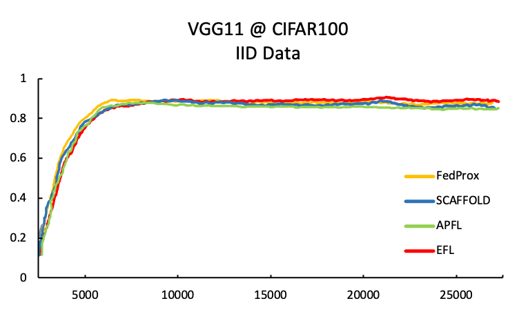
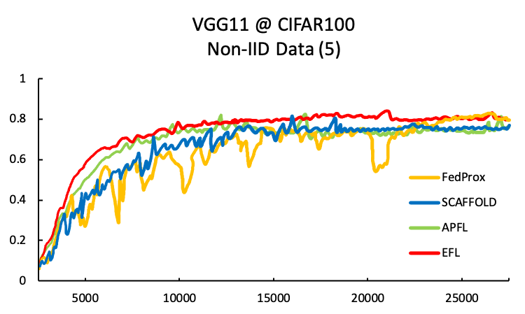
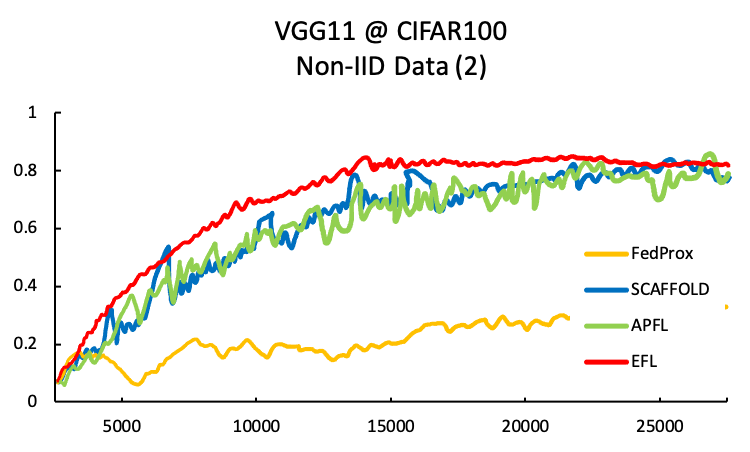
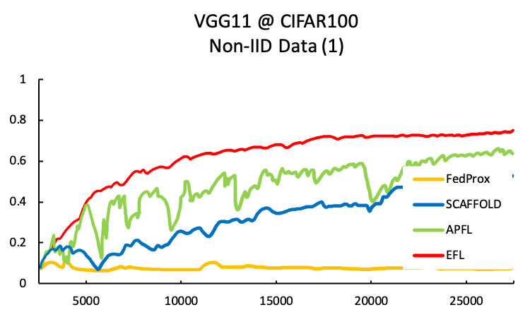
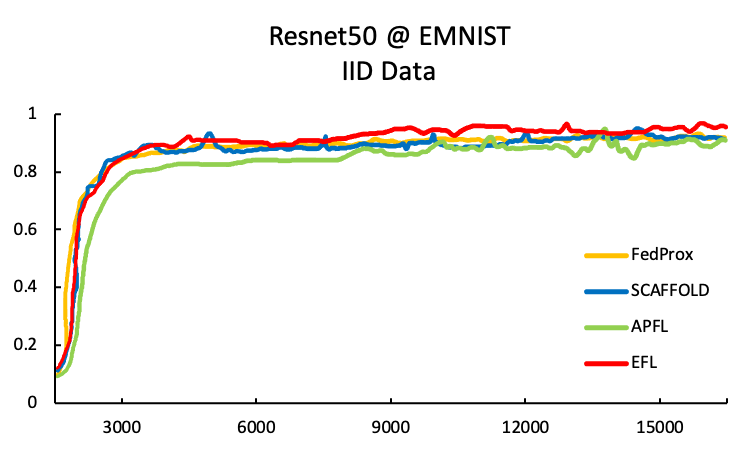
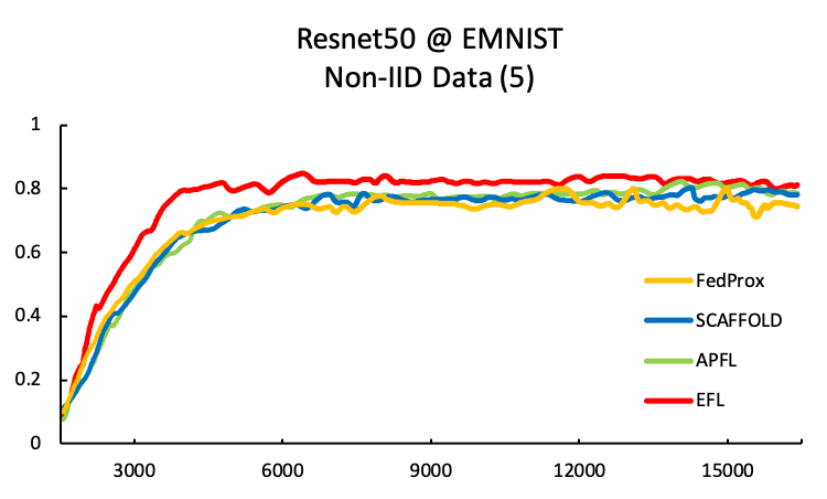
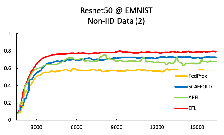
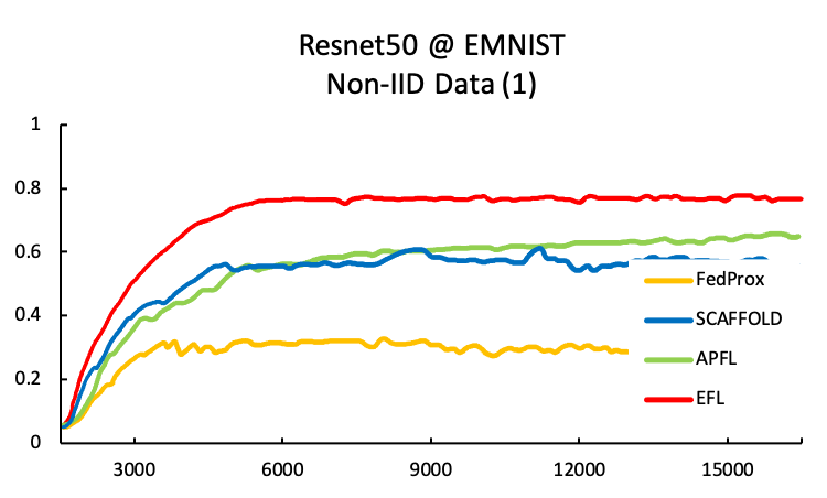
Figure 1: Testing Accuracy-Communication Rounds comparisons of VGG11 on CIFAR100 and Resnet50 on EMNIST in a distributed setting for IID and non-IID data. In the non-IID cases, every client only holds examples from exactly $m$ classes in the dataset. All methods suffer from degraded convergence speed in the non-IID situation, but EFL is affected by far the least.

4.1 Inactive Client

If there exist inactive clients, the convergence rate changes to $O(\frac{\sum_{t=0}^{\tau-1}y_{t}J}{\tau E+E^{2}})$. $y_{t}$ indicates if there are inactive clients in the $t$-th round. Furthermore, the term converges to zero if $y_{t}\in O(\tau)$, which means that a mild degree of inactive client will not discourage the convergence. A client can frequently become inactive due to the limited resources in reality. Permanently removing the client in this case may improve the model performance. Specially, we will remove the client if the system without this client leads to a smaller training loss when it terminates at the deadline $T$.

Suppose a client $a$ is inactive with the probability $0<y^{a}<1$ in each round, and let $f_{0}(\tau)$ be the convergence bound if we keep the client, $f_{1}(\tau)$ be the bound if it is abandoned at $\tau_{0}$. For $f_{0}$ with sufficiently many steps, the first term in Equation (7) shrinks to zero, and the second term converges to $y^{a}J$. Thus, $f_{0}\approx y^{a}J$, and we can obtain that $f_{1}{\tau}=\frac{\widetilde{C}_{\tau}}{(E(\tau-\tau_{0})+\widetilde{\gamma})^{2}}$ for some $\widetilde{C}_{\tau}$ and $\widetilde{\gamma}$, thus we have

Corollary 1.

An inactive client a should be abandoned if

$$y^{a}J>f_{1}(T).$$ (8)

Assuming $C_{\tau}\approx\widetilde{C}_{\tau}=\tau C$ and $\gamma\approx\widetilde{\gamma}$, i.e., the removed client does not significantly affect the overall SGD variance and the degree of non-IID, then Equation (8) can be formulated as

$$y^{k}>O(\frac{\frac{C}{J}}{TE}).$$ (9)

From Corollary 1, the more epochs the training on the local client, the more sensitive it is to the in-activeness.

4.2 Incomplete Client

Based on Theorem 1, the convergence bound is controlled by the expectation of $p_{\tau}^{k}$ and its functions. EFL allows clients to upload partial work with adaptive weight $p_{\tau}^{k}=\frac{Ep^{k}}{s_{\tau}^{k}}$. It assigns a greater aggregation coefficient to clients that complete fewer local epochs, and turns out to guarantee the convergence in the non-IID setting. The resulting convergence bound follows $O(\frac{E^{5}\sum_{t=0}^{\tau-1}\sum_{k}^{N}p^{k}\mathbb{E}[1/s_{t}^{k}]+E^{2}\sum_{t=0}^{\tau-1}\sum_{k}^{N}(p^{k}\sigma_{k})^{2}\mathbb{E}[1/s_{t}^{k}]}{(\tau E+E^{2})^{2}})$.

The reason for enlarging the aggregation coefficient lies in Equation (6) that increasing $p_{\tau}^{k}$ is equivalent to increasing the learning rate of client $k$. By assigning clients that complete fewer epochs a greater aggregation coefficient, these clients effectively run further in each local step, compensating for less epochs.

Table 2: BMTA for the non-IID data setting

Methods	MNIST	CIFAR100	Sent140	Shakes.
FedAvg	$98.30$	$2.27$	$59.14$	$51.35$
FedGATE	99.15	$80.94$	$68.84$	$54.71$
VRL-SGD	$98.86$	$2.81$	$68.62$	$52.33$
APFL	$98.49$	$77.19$	$68.81$	$55.27$
FedAMP	$99.06$	$81.17$	69.01	$58.42$
EFL	$99.10$	81.38	$68.95$	60.49

4.3 Client Departure

If $k$-th client quits at $\tau_{0}<T$, no more updates will be received from it, and $s_{\tau}^{k}=0$ for all $\tau>\tau_{0}$. As a result, the value of ratio $\frac{\mathbb{E}[p_{\tau}^{k}s_{\tau}^{k}]}{p^{k}}$ is different for different $k$, and $r_{\tau}=1$ for all $\tau>\tau_{0}$. According to Theorem 1, $\omega_{\tau E}^{G}$ cannot converge to the global optimal $\omega^{*}$ as $H_{T}\geq T-\tau_{0}$. Intuitively, a client should contribute sufficiently many updates in order for its features to be captured by the trained model in the non-IID setting. After a client leaves, the remaining training steps will not keep much memory as it runs more rounds. Thus, the model may not be applicable to the leaving client, especially when it leaves early in the training ($\tau_{0}\ll T$), which indicates that we may discard a departing client if we cannot guarantee the trained model performs well on it, and the earlier a client leaves, the more likely it should be discarded.

However, removing the departing client (the $a$ client) from the training may push the original learning objective $F=\sum_{k=1}^{N}p^{k}\widetilde{F}_{k}$ towards the new one $\hat{F}=\sum_{k=1,k\neq a}^{N}p^{k}\widetilde{F}_{k}$, and the optimal weight $\omega^{*}$ will also shift to some $\hat{\omega}^{*}$ that minimizes $\hat{F}$. There exists a gap between these two optimal, which further adds an additional term to the convergence bound obtained in Theorem 1, and a sufficient number of updates are required for $\omega_{\tau E}^{G}$ to converge to the new optimal $\hat{\omega}^{*}$.

4.4 Client Arrival

The same argument holds when a new client joins in the training, which requires changing the original global objective to include the loss on the new client’s data. The learning rate also needs to be increased when the objective changes. Intuitively, if the shift happens at a large time $\tau_{0}$, where $\omega_{\tau E}^{G}$ approaches to the old optimal $\omega^{*}$ and $\eta_{\tau_{0}}$ is close to zero, reducing the latest differences $||\omega_{\tau E}^{G}-\hat{\omega}^{*}||^{2}\approx||\omega^{*}-\hat{\omega}^{*}||^{2}$ with a small learning rate is inapplicable. Thus, a greater learning rate should be adopted, which is equivalent to initiate a fresh start after the shift, and there still needs more updating rounds to fully address the new client.

We also present the bounds of the additional term due to the objective shift as

Theorem 2.

For the global objective shift $F\rightarrow\hat{F}$, $\omega^{*}\rightarrow\hat{\omega}^{*}$, let $\hat{D}_{k}=F_{k}(\hat{\omega}^{*})-F_{k}^{*}$ quantify the degree of non-IID data with respect to the new objective. If the client $a$ quits the system,

$$||\omega^{*}-\hat{\omega}^{*}||^{2}\leq\frac{8Ln_{a}^{2}\hat{D}_{a}}{\mu^{2}n^{2}}.$$ (10)

If the client $a$ joins the system,

$$||\omega^{*}-\hat{\omega}^{*}||^{2}\leq\frac{8Ln_{a}^{2}\hat{D}_{a}}{\mu^{2}(n+n_{a})^{2}},$$ (11)

where $n$ is the total number of samples before the shift.

It can be concluded that the bound reduces when the data becomes more IID, and when the changed client owns fewer data samples.

5 Experiments

In this section, we first demonstrate the effectiveness and efficiency of EFL in the non-IID data setting, and compare with several baseline algorithms. Then, we show the robustness of EFL on the low participation rate challenge.

5.1 Experimental Settings

Both convex and non-convex models are evaluated on a number of benchmark datasets of federated learning. Specifically, we adopt MNIST LeCun et al. (1998), EMNIST Cohen et al. (2017) dataset with Resnet50 He et al. (2016), CIFAR100 dataset Krizhevsky et al. (2009) with VGG11 Simonyan and Zisserman (2014) network, Shakespeare dataset with an LSTM McMahan et al. (2017a)to predict the next character, Sentiment140 dataset Go et al. (2009) with an LSTM to classify sentiment and synthetic dataset with a linear regression classifier.

Our experiments are conducted on the TensorFlow platform running in a Linux server. For reference, statistics of datasets, implementation details and the anonymized code are summarized in supplementary material.

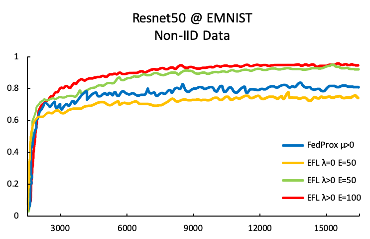
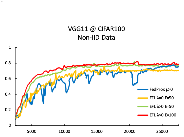
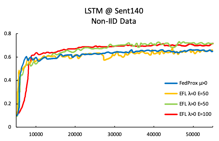
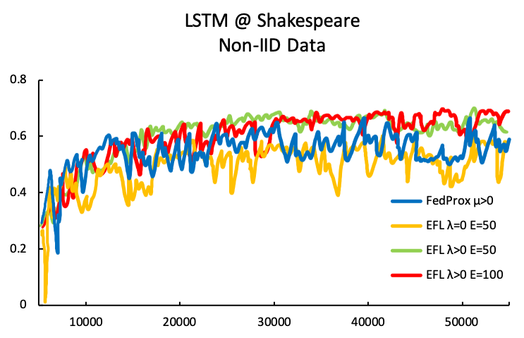
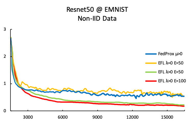
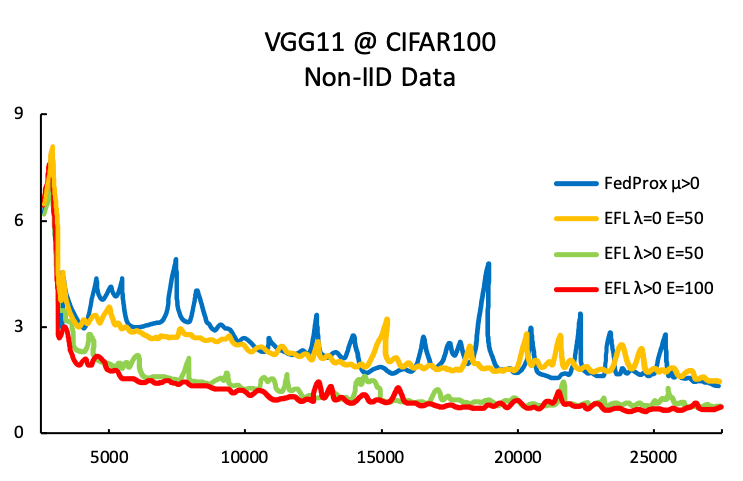
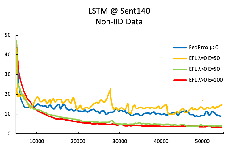
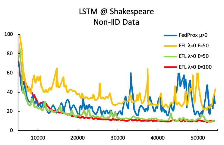
Figure 2: The first row shows Testing Accuracy-Communication Rounds comparison and the second row shows Training Loss-Communication Rounds comparison in non-IID setting. EFL with elastic term stabilizes and improves the convergence of the algorithm.

5.2 Effects of Non-IID Data

We run experiments with a simplified version of the well-studied 11-layer VGG11 network, which we train on the CIFAR100 dataset in a federated learning setup using 100 clients. For the IID setting, we split the training data randomly into equally sized shards and assign one shard to every clients. For the non-IID ($m$) setting, we assign every client samples from exactly $m$ classes of the dataset. We also perform experiments with Resnet50, where we train on EMNIST dataset under the same setup of the federated learning environment. Both models are trained using SGD.

Figure 1 shows the convergence comparison in terms of gradient evaluations for the two models using different algorithms. FedProx Li et al. (2018) incorporates a proximal term in local objective to improve the model performance on the non-IID data, SCAFFOLD Karimireddy et al. (2020b) adopts control variate to alleviate the effects of data heterogeneity, and APFL Deng et al. (2020) learns personalized local models to mitigate heterogeneous data on clients.

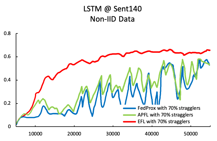
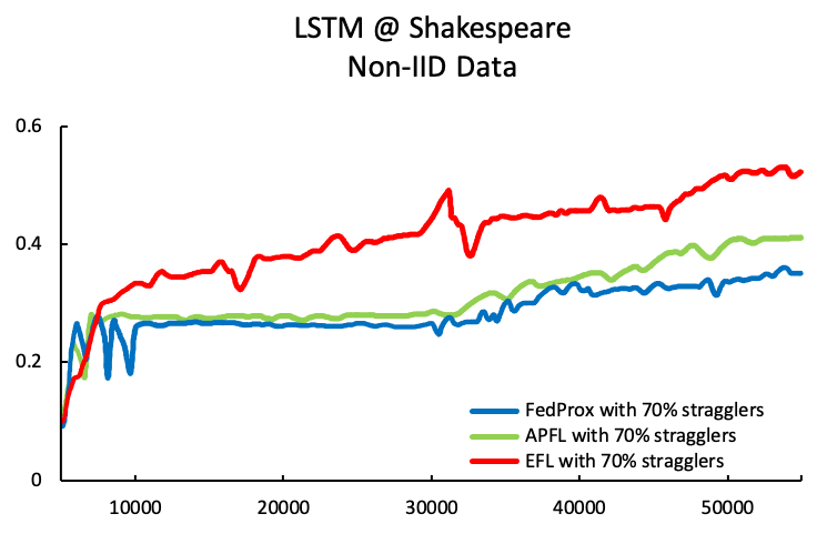
Figure 3: Testing Accuracy-Communication Rounds comparisons among different algorithms in low participation rate. EFL utilizes incomplete updates from stragglers and is robust to the low participation rate.

We observe that while all methods achieve comparably fast convergence in terms of gradient evaluations on IID data, they suffer considerably in the non-IID setting. From left to right, as data becomes more non-IID, convergence becomes worse for FedProx, and it can diverge in some cases. SCAFFOLD and APFL exhibit its ability in alleviating the data heterogeneity, but are not stable during training. As this trend can be observed also for Resnet50 on EMNIST case, it can be concluded that the performance loss that is originated from the non-IID data is not unique to some functions.

Aiming at better illustrating the effectiveness of the proposed algorithm, we further evaluate and compare EFL with the state-of-the-art algorithms, including FedGATE Haddadpour et al. (2021), VRL-SGD Liang et al. (2019), APFL Deng et al. (2020) and FedAMP Huang et al. (2021) on MNIST, CIFAR100, Sentiment140, and Shakespeare dataset. The performance of all the methods is evaluated by the best mean testing accuracy (BMTA) in percentage, where the mean testing accuracy is the average of the testing accuracy on all participants. For each of datasets, we apply a non-IID data setting.

Table 2 shows the BMTA of all the methods under non-IID data setting, which is not easy for vanilla algorithm FedAvg. On the challenging CIFAR100 dataset, VRL-SGD is unstable and performs catastrophically because the models are destroyed such that the customized gradient updates in the method can not tune it up. APFL and FedAMP train personalized models to alleviate the non-IID data, however, the performance of APFL is still damaged by unstable training. FedGATE, FedAMP and EFL achieve comparably good performance on all datasets.

5.3 Effects of the Elastic Term

EFL utilizes the incomplete local updates, which indicates that clients may perform different amount of local work $s_{\tau}^{k}$, and this parameter together with the elastic term scaled by $\lambda$ affect the performance of the algorithm. However, $s_{\tau}^{k}$ is determined by its constrains, i.e., it is a client specific parameter, EFL can only set the maximum number of local epochs to prevent local models drifting too far away from the global model, and tune a best $\lambda$. Intuitively, a proper $\lambda$ restricts the optimization trajectory by limiting the most informative parameters’ change, and guarantees the convergence.

We explore impacts of the elastic term by setting different values of $\lambda$, and investigate whether the maximum number of local epochs influences the convergence behavior of the algorithm. Figure 2 shows the performance comparison on different datasets using different models. We compare the result between EFL with $\lambda=0$ and EFL with best $\lambda$. For all datasets, it can be observed that the appropriate $\lambda$ can increase the stability for unstable methods and can force divergent methods to converge, and it also increases the accuracy in most cases. As a result, setting $\lambda\geq 0$ is particularly useful in the non-IID setting, which indicates that the EFL benefits practical federated settings.

5.4 Robustness of EFL

Finally, in Figure 3, we demonstrate that EFL is robust to the low participation rate. In particular, we track the convergence speed of LSTM trained on Sentiment140 and Shakespeare dataset. It can be observed that reducing the participation rate has negative effects on all methods. The causes for these negative effects, however, are different: In FedAvg, the actual participation rate is determined by the number of clients that finish the complete training process, because it does not include the incomplete updates. This can steer the optimization process away from the minimum and might even cause catastrophic forgetting. On the other hand, low participation rate reduces the convergence speed of EFL by causing the clients residuals to go out sync and increasing the gradient staleness. The more rounds a client has to wait before it is selected to participate in training again, the more outdated the accumulated gradients become.

6 Conclusion

In this paper, we propose EFL as an unbiased FL algorithm that can adapt to the statistical diversity issue by making the most informative parameters less volatile. EFL can be understood as an alternative paradigm for fair FL, which tackles bias that is originated from the non-IID data and the low participation rate. Theoretically, we provide convergence guarantees for EFL when training on the non-IID data at the low participation rate. Empirically, experiments support the competitive performance of the algorithm on the robustness and efficiency.

References

- Agarwal et al. [2018] Naman Agarwal, Ananda Theertha Suresh, Felix Yu, Sanjiv Kumar, and H Brendan Mcmahan. cpsgd: Communication-efficient and differentially-private distributed sgd. arXiv preprint arXiv:1805.10559, 2018.
- Aji and Heafield [2017] Alham Fikri Aji and Kenneth Heafield. Sparse communication for distributed gradient descent. arXiv preprint arXiv:1704.05021, 2017.
- Alistarh et al. [2017] Dan Alistarh, Demjan Grubic, Jerry Li, Ryota Tomioka, and Milan Vojnovic. Qsgd: Communication-efficient sgd via gradient quantization and encoding. In Advances in Neural Information Processing Systems, pages 1709–1720, 2017.
- Basu et al. [2019] Debraj Basu, Deepesh Data, Can Karakus, and Suhas Diggavi. Qsparse-local-sgd: Distributed sgd with quantization, sparsification, and local computations. arXiv preprint arXiv:1906.02367, 2019.
- Bernstein et al. [2018] Jeremy Bernstein, Yu-Xiang Wang, Kamyar Azizzadenesheli, and Anima Anandkumar. signsgd: Compressed optimisation for non-convex problems. arXiv preprint arXiv:1802.04434, 2018.
- Cohen et al. [2017] Gregory Cohen, Saeed Afshar, Jonathan Tapson, and Andre Van Schaik. Emnist: Extending mnist to handwritten letters. In 2017 International Joint Conference on Neural Networks (IJCNN), pages 2921–2926. IEEE, 2017.
- Dai et al. [2019] Xinyan Dai, Xiao Yan, Kaiwen Zhou, Han Yang, Kelvin KW Ng, James Cheng, and Yu Fan. Hyper-sphere quantization: Communication-efficient sgd for federated learning. arXiv preprint arXiv:1911.04655, 2019.
- Deng et al. [2020] Yuyang Deng, Mohammad Mahdi Kamani, and Mehrdad Mahdavi. Adaptive personalized federated learning. arXiv preprint arXiv:2003.13461, 2020.
- Draelos et al. [2017] Timothy J Draelos, Nadine E Miner, Christopher C Lamb, Jonathan A Cox, Craig M Vineyard, Kristofor D Carlson, William M Severa, Conrad D James, and James B Aimone. Neurogenesis deep learning: Extending deep networks to accommodate new classes. In 2017 International Joint Conference on Neural Networks (IJCNN), pages 526–533. IEEE, 2017.
- Duchi et al. [2014] John C Duchi, Michael I Jordan, and Martin J Wainwright. Privacy aware learning. Journal of the ACM (JACM), 61(6):1–57, 2014.
- Go et al. [2009] Alec Go, Richa Bhayani, and Lei Huang. Twitter sentiment classification using distant supervision. CS224N project report, Stanford, 1(12):2009, 2009.
- Haddadpour and Mahdavi [2019] Farzin Haddadpour and Mehrdad Mahdavi. On the convergence of local descent methods in federated learning. arXiv preprint arXiv:1910.14425, 2019.
- Haddadpour et al. [2021] Farzin Haddadpour, Mohammad Mahdi Kamani, Aryan Mokhtari, and Mehrdad Mahdavi. Federated learning with compression: Unified analysis and sharp guarantees. In International Conference on Artificial Intelligence and Statistics, pages 2350–2358. PMLR, 2021.
- He et al. [2016] Kaiming He, Xiangyu Zhang, Shaoqing Ren, and Jian Sun. Deep residual learning for image recognition. In Proceedings of the IEEE conference on computer vision and pattern recognition, pages 770–778, 2016.
- Huang et al. [2021] Yutao Huang, Lingyang Chu, Zirui Zhou, Lanjun Wang, Jiangchuan Liu, Jian Pei, and Yong Zhang. Personalized cross-silo federated learning on non-iid data. In Proceedings of the AAAI Conference on Artificial Intelligence, 2021.
- Kairouz et al. [2019] Peter Kairouz, H Brendan McMahan, Brendan Avent, Aurélien Bellet, Mehdi Bennis, Arjun Nitin Bhagoji, Keith Bonawitz, Zachary Charles, Graham Cormode, Rachel Cummings, et al. Advances and open problems in federated learning. arXiv preprint arXiv:1912.04977, 2019.
- Karimireddy et al. [2020a] Sai Praneeth Karimireddy, Martin Jaggi, Satyen Kale, Mehryar Mohri, Sashank J Reddi, Sebastian U Stich, and Ananda Theertha Suresh. Mime: Mimicking centralized stochastic algorithms in federated learning. arXiv preprint arXiv:2008.03606, 2020.
- Karimireddy et al. [2020b] Sai Praneeth Karimireddy, Satyen Kale, Mehryar Mohri, Sashank Reddi, Sebastian Stich, and Ananda Theertha Suresh. Scaffold: Stochastic controlled averaging for federated learning. In International Conference on Machine Learning, pages 5132–5143. PMLR, 2020.
- Khaled et al. [2020] Ahmed Khaled, Konstantin Mishchenko, and Peter Richtárik. Tighter theory for local sgd on identical and heterogeneous data. In International Conference on Artificial Intelligence and Statistics, pages 4519–4529. PMLR, 2020.
- Kirkpatrick et al. [2017] James Kirkpatrick, Razvan Pascanu, Neil Rabinowitz, Joel Veness, Guillaume Desjardins, Andrei A Rusu, Kieran Milan, John Quan, Tiago Ramalho, Agnieszka Grabska-Barwinska, et al. Overcoming catastrophic forgetting in neural networks. Proceedings of the national academy of sciences, 114(13):3521–3526, 2017.
- Konečnỳ et al. [2016] Jakub Konečnỳ, H Brendan McMahan, Felix X Yu, Peter Richtárik, Ananda Theertha Suresh, and Dave Bacon. Federated learning: Strategies for improving communication efficiency. arXiv preprint arXiv:1610.05492, 2016.
- Krizhevsky et al. [2009] Alex Krizhevsky, Geoffrey Hinton, et al. Learning multiple layers of features from tiny images. 2009.
- LeCun et al. [1998] Yann LeCun, Léon Bottou, Yoshua Bengio, and Patrick Haffner. Gradient-based learning applied to document recognition. Proceedings of the IEEE, 86(11):2278–2324, 1998.
- Li et al. [2018] Tian Li, Anit Kumar Sahu, Manzil Zaheer, Maziar Sanjabi, Ameet Talwalkar, and Virginia Smith. Federated optimization in heterogeneous networks. arXiv preprint arXiv:1812.06127, 2018.
- Li et al. [2019] Xiang Li, Kaixuan Huang, Wenhao Yang, Shusen Wang, and Zhihua Zhang. On the convergence of fedavg on non-iid data. arXiv preprint arXiv:1907.02189, 2019.
- Li et al. [2020a] Tian Li, Anit Kumar Sahu, Ameet Talwalkar, and Virginia Smith. Federated learning: Challenges, methods, and future directions. IEEE Signal Processing Magazine, 37(3):50–60, 2020.
- Li et al. [2020b] Zhize Li, Dmitry Kovalev, Xun Qian, and Peter Richtárik. Acceleration for compressed gradient descent in distributed and federated optimization. arXiv preprint arXiv:2002.11364, 2020.
- Liang et al. [2019] Xianfeng Liang, Shuheng Shen, Jingchang Liu, Zhen Pan, Enhong Chen, and Yifei Cheng. Variance reduced local sgd with lower communication complexity. arXiv preprint arXiv:1912.12844, 2019.
- Lin et al. [2018] Tao Lin, Sebastian U Stich, Kumar Kshitij Patel, and Martin Jaggi. Don’t use large mini-batches, use local sgd. arXiv preprint arXiv:1808.07217, 2018.
- McMahan et al. [2017a] Brendan McMahan, Eider Moore, Daniel Ramage, Seth Hampson, and Blaise Aguera y Arcas. Communication-efficient learning of deep networks from decentralized data. In Artificial Intelligence and Statistics, pages 1273–1282. PMLR, 2017.
- McMahan et al. [2017b] H Brendan McMahan, Daniel Ramage, Kunal Talwar, and Li Zhang. Learning differentially private recurrent language models. arXiv preprint arXiv:1710.06963, 2017.
- Parisi et al. [2018] German I Parisi, Jun Tani, Cornelius Weber, and Stefan Wermter. Lifelong learning of spatiotemporal representations with dual-memory recurrent self-organization. Frontiers in neurorobotics, 12:78, 2018.
- Reisizadeh et al. [2020] Amirhossein Reisizadeh, Aryan Mokhtari, Hamed Hassani, Ali Jadbabaie, and Ramtin Pedarsani. Fedpaq: A communication-efficient federated learning method with periodic averaging and quantization. In International Conference on Artificial Intelligence and Statistics, pages 2021–2031. PMLR, 2020.
- Rusu et al. [2016] Andrei A Rusu, Neil C Rabinowitz, Guillaume Desjardins, Hubert Soyer, James Kirkpatrick, Koray Kavukcuoglu, Razvan Pascanu, and Raia Hadsell. Progressive neural networks. arXiv preprint arXiv:1606.04671, 2016.
- Sahu et al. [2018] Anit Kumar Sahu, Tian Li, Maziar Sanjabi, Manzil Zaheer, Ameet Talwalkar, and Virginia Smith. On the convergence of federated optimization in heterogeneous networks. arXiv preprint arXiv:1812.06127, 3, 2018.
- Shin et al. [2017] Hanul Shin, Jung Kwon Lee, Jaehong Kim, and Jiwon Kim. Continual learning with deep generative replay. In Advances in neural information processing systems, pages 2990–2999, 2017.
- Simonyan and Zisserman [2014] Karen Simonyan and Andrew Zisserman. Very deep convolutional networks for large-scale image recognition. arXiv preprint arXiv:1409.1556, 2014.
- Soltoggio [2015] Andrea Soltoggio. Short-term plasticity as cause–effect hypothesis testing in distal reward learning. Biological cybernetics, 109(1):75–94, 2015.
- Stich [2018] Sebastian U Stich. Local sgd converges fast and communicates little. arXiv preprint arXiv:1805.09767, 2018.
- Tsuzuku et al. [2018] Yusuke Tsuzuku, Hiroto Imachi, and Takuya Akiba. Variance-based gradient compression for efficient distributed deep learning. arXiv preprint arXiv:1802.06058, 2018.
- Wang and Joshi [2018] Jianyu Wang and Gauri Joshi. Cooperative sgd: A unified framework for the design and analysis of communication-efficient sgd algorithms. arXiv preprint arXiv:1808.07576, 2018.
- Zhao et al. [2018] Yue Zhao, Meng Li, Liangzhen Lai, Naveen Suda, Damon Civin, and Vikas Chandra. Federated learning with non-iid data. arXiv preprint arXiv:1806.00582, 2018.
- Zhou and Cong [2017] Fan Zhou and Guojing Cong. On the convergence properties of a -step averaging stochastic gradient descent algorithm for nonconvex optimization. arXiv preprint arXiv:1708.01012, 2017.
- Zhu et al. [2020] Wennan Zhu, Peter Kairouz, Brendan McMahan, Haicheng Sun, and Wei Li. Federated heavy hitters discovery with differential privacy. In International Conference on Artificial Intelligence and Statistics, pages 3837–3847. PMLR, 2020.