Taming Nonconvexity in Kernel Feature Selection—Favorable Properties of the Laplace Kernel

Abstract.

Kernel-based feature selection is an important tool in nonparametric statistics. Despite many practical applications of kernel-based feature selection, there is little statistical theory available to support the method. A core challenge is the objective function of the optimization problems used to define kernel-based feature selection are nonconvex. The literature has only studied the statistical properties of the global optima, which is a mismatch, given that the gradient-based algorithms available for nonconvex optimization are only able to guarantee convergence to local minima. Studying the full landscape associated with kernel-based methods, we show that feature selection objectives using the Laplace kernel (and other $\ell_{1}$ kernels) come with statistical guarantees that other kernels, including the ubiquitous Gaussian kernel (or other $\ell_{2}$ kernels) do not possess. Based on a sharp characterization of the gradient of the objective function, we show that $\ell_{1}$ kernels eliminate unfavorable stationary points that appear when using an $\ell_{2}$ kernel. Armed with this insight, we establish statistical guarantees for $\ell_{1}$ kernel-based feature selection which do not require reaching the global minima. In particular, we establish model-selection consistency of $\ell_{1}$-kernel-based feature selection in recovering main effects and hierarchical interactions in the nonparametric setting with $n\sim\log p$ samples.

1. Introduction

Statistical learning problems are often characterized by data sets in which both the number of data points, $n$, and the number of dimensions, $p$, are large. Such scaling is increasingly common in applied problem domains, and it is often accompanied by a focus on prediction and flexible nonparametric models in such domains. Examples of such problem domains include text classification, object recognition, and genetic screening [LCW⁺17, CLWY18, DR20]. Even in such domains, however, there is a tension between prediction and interpretation [AHM⁺17, Rud19], and increasingly a call for “white-box” nonparametric modeling, where effective prediction and interpretability are both required [GMR⁺18, MSK⁺19, Mil19].

One general approach to addressing this challenge involves the use of kernel-based feature selection. Kernel-based methods are nonparametric and yet have mathematical structure that can be exploited for interpretability. In particular algorithms, kernel-based feature selection methods have the advantage of being able to find reduced-dimensional representations of regression functions, while capturing nonlinear relationships between the features and response. Moreover, kernel-based feature selection methods are expressed as objective functions in an optimization framework, and blend appealingly with the modern focus on gradient-based optimization methods for fitting models. Two main objectives have become dominant in the literature on kernel-based feature selection:

1. Hilbert-Schmidt Independence Criterion (HSIC). This is a nonparametric dependence measure based on the Hilbert-Schmidt norm of a covariance operator [GBSS05]. This dependence measure can be used for feature selection in the following way [SSG⁺07, SSG⁺12]. Let $(X,Y)$ denote the data where $X\in\mathbb{R}^{p}$ is the feature vector and $Y\in\mathbb{R}$ is the response. Let $k(x,x^{\prime})$ be a positive definite kernel. For any vector $x\in\mathbb{R}^{p}$ and any subset $\mathcal{T}\subseteq\{1,2,\ldots,p\}$, denote $x^{\mathcal{T}}\in\mathbb{R}^{p}$ with components $x_{i}^{\mathcal{T}}=x_{i}$ if $i\in\mathcal{T}$ and let $x_{i}^{\mathcal{T}}=0$ if $i\not\in\mathcal{T}$. Let $(X^{\prime},Y^{\prime})$ denote an independent copy of $(X,Y)$. The HSIC-based approach to feature selection finds a subset of features by optimizing

   $$\begin{split}\mathop{\rm maximize}_{\mathcal{T}:\mathcal{T}\subseteq\{1,2,\ldots,p\}}~{}~{}&{\rm HSIC}(\mathcal{T})\\ \text{where}~{}~{}~{}~{}&{\rm HSIC}(\mathcal{T})=\mathbb{E}[YY^{\prime}k(X^{\mathcal{T}},(X^{\prime})^{\mathcal{T}})].\end{split}$$

   Subsequent work studied continuous relaxations of this objective [MFD10, YJS⁺14]. Most of the focus in this literature is, however, computational, and there are currently no general statistical guarantees available for the HSIC-based approach.

2. Kernel ridge regression (KRR). In this framework the features are multiplied by a set of weights (either discrete or continuous), and the following objective is formed [WMC⁺00, GC02, CSS⁺07, All13, CSWJ17]:

   $$\begin{split}\mathop{\rm minimize}_{\mathcal{T}:\mathcal{T}\subseteq\{1,2,\ldots,p\}}~{}~{}&{\rm KRR}(\mathcal{T})\\ \text{where}~{}~{}~{}~{}&{\rm KRR}(\mathcal{T})=\frac{1}{2}\mathbb{E}[(Y-f(X^{\mathcal{T}}))^{2}]+\frac{\lambda}{2}\left\|{f}\right\|_{\mathcal{H}}^{2},\end{split}$$

   where $\left\|{\cdot}\right\|_{\mathcal{H}}$ denotes the norm of $\mathcal{H}$, a reproducing kernel Hilbert space. This objective is optimized jointly over the weights and the regression function. [CSWJ17] prove that the global optima of the KRR objective are feature-selection consistent. No statistical guarantees are available for continuous relaxations of the discrete objective.

Both of the discrete and continuous HSIC and KRR objectives are nonconvex. The difficulty of analyzing such nonconvex objectives has led to a lack of understanding of the statistical properties of the resulting feature-selection algorithms. Indeed, for HSIC, the most recent work has been disappointing—it has been shown via counterexamples that the global optima of the HSIC objective (discrete or continuous) can fail to select important features and the overall procedure is therefore inconsistent [LR20]. The picture is slightly more favorable for KRR, in that the global optima of the discrete objective is selection consistent; however, this is the lone guarantee available in the literature [CSWJ17]. No other guarantees exist regarding the local optima or stationary points for any continuous relaxation of the KRR objective—yet these relaxations are the most critical to algorithmic success in practice.

Our work studies the landscape of the continuous KRR objective, most notably we study all of the stationary points (not simply the global optima). Despite the nonconvexity of the objective, we show that, with a carefully designed kernel, such stationary point have provably benign statistical guarantees. Formally, assuming without loss of generality that $\mathbb{E}[Y]=0$ (an assumption that we make throughout the paper), in this paper we consider minimizing the following form of KRR-based objective:

$$\begin{split}\mathop{\rm minimize}_{\beta:\beta\geq 0,\left\|{\beta}\right\|_{1}\leq M}~{}~{}&\mathcal{J}_{\gamma}(\beta):=\mathcal{J}(\beta)+\gamma\left\|{\beta}\right\|_{1}\\ ~{}~{}\text{where}~{}~{}&\mathcal{J}(\beta)=\min_{f\in\mathcal{H}}~{}\frac{1}{2}\mathbb{E}\left[(Y-f(\beta^{1/q}\odot X))^{2}\right]+\frac{\lambda}{2}\left\|{f}\right\|_{\mathcal{H}}^{2},\end{split}$$ (1.1)

and where $\lambda,\gamma,M\geq 0$ are regularization parameters. Above we use the notation shorthand $(\beta^{1/q}\odot X)=(\beta^{1/q}X_{1},\beta_{2}^{1/q}X_{2},\ldots,\beta_{p}^{1/q}X_{p})$ for a vector $\beta\in\mathbb{R}_{+}^{p}$. We take the reproducing kernel Hilbert space (RKHS) $\mathcal{H}$ to be of $\ell_{q}$ type, where $q=1,2$, meaning that the kernel $k$ associated with the RKHS $\mathcal{H}$ in the objective takes the form $k(x,x^{\prime})=h(\left\|{x-x^{\prime}}\right\|_{q}^{q})$, where the notation $\left\|{z}\right\|_{q}$ refers to the Euclidean $\ell_{q}$ norm of a vector $z$. Examples of the $\ell_{q}$ type RKHS include the Gaussian RKHS, where $k(x,x^{\prime})=\exp(-\left\|{x-x^{\prime}}\right\|_{2}^{2})$, and the Laplace RKHS, where $k(x,x^{\prime})=\exp(-\left\|{x-x^{\prime}}\right\|_{1})$. One of our major findings is the choice of the $\ell_{1}$ kernel (e.g., the Laplace kernel) rather than an $\ell_{2}$ kernel (e.g., the Gaussian) yields significant improvements to the landscape of the (nonconvex) objective function (both the population case and the finite-sample case). This is suggested by the following example, which shows how the choice of an $\ell_{1}$ kernel eliminates bad stationary points that would otherwise appear for an $\ell_{2}$ kernel.

Example  Consider an additive model where the response $Y$ is the sum of individual independent main effects, $f_{i}^{*}(X_{i})$; i.e., $Y=\sum_{i=1}^{p}f^{*}_{i}(X_{i})$, where $X_{1}\perp X_{2}\perp\ldots\perp X_{p}$. Consider the KRR objective function $\mathcal{J}(\beta)$ (see equation (1.1)). We have the following description of the population landscape of the KRR objective $\mathcal{J}(\beta)$:

• For $q=1,2$, the global minimum of $\mathcal{J}(\beta)$ satisfies $\beta_{j}>0$ for all $1\leq j\leq p$.

• For $q=1$, any stationary point $\beta$ of $\mathcal{J}(\beta)$ satisfies $\beta_{j}>0$ for all $1\leq j\leq p$.

• For $q=2$, $\beta=0$ is a stationary point if ${\rm Cov}(f_{j}^{*}(X_{j}),X_{j})=0$ for all $1\leq j\leq p$.

• For $q=2$, there is a stationary point $\beta$ with $\beta_{j}=0$ if ${\rm Cov}(f_{j}^{*}(X_{j}),X_{j}^{r})=0$ for $r=1,2$.

Under the additive model considered in the example, all the features are important. Thus we would like our feature selection algorithm to converge to some $\beta$ such that $\beta_{j}>0$ for all $j\in[p]$. Our example shows, however, that although the global minimum for both $\ell_{1}$ and $\ell_{2}$ kernels satisfy this desideratum, a gradient-descent algorithm may become trapped at a bad stationary point (where $\beta_{j}=0$ for some $j$) if one uses an $\ell_{2}$ kernel. This does not occur if one uses an $\ell_{1}$ kernel.

The previous example demonstrates the clear advantage of the $\ell_{1}$ kernel over the $\ell_{2}$ kernel in the context of an additive model. This same advantage in fact holds under more general models. We sketch why this is the case—why the $\ell_{1}$ type RKHS leads to a better objective landscape than the $\ell_{2}$ type RKHS—with formal details to follow in subsequent sections. The key to our result is a sharp characterization of the gradient of the KRR objective $\nabla_{\beta}\mathcal{J}(\beta)$ in the context of any joint distribution for $(X,Y)$. Let $f_{\beta}$ be the minimum of the KRR in equation (1.1), and let $r_{\beta}$ denote the residual, $r_{\beta}(x,y)=y-f_{\beta}(x)$. Equations (1.2) and (1.3) characterize the leading terms of the gradient. Letting $\bar{\mu}$ denote a measure implicitly determined solely by the kernel $k$, we have the following characterization of the gradient $\nabla_{\beta}\mathcal{J}(\beta)$ (below $o_{\lambda}(1)$ denotes a quantity that tends to $0$ as $\lambda$ tends to $0$):

• For $q=1$, the gradient of the objective $\nabla\mathcal{J}(\beta)$ takes the form

  $$\partial_{\beta_{l}}\mathcal{J}(\beta)=-\frac{1}{\lambda}\left(\iint\left|{\rm Cov}\left(r_{\beta}(\beta\odot X,Y)e^{i\langle\beta\odot X,\omega\rangle},e^{i\zeta_{l}X_{l}}\right)\right|^{2}\cdot\frac{d\zeta_{l}}{\pi\zeta_{l}^{2}}\cdot\bar{\mu}(d\omega)+o_{\lambda}(1)\right).$$ (1.2)

• For $q=2$, the gradient of the objective $\nabla\mathcal{J}(\beta)$ takes the form

  $$\partial_{\beta_{l}}\mathcal{J}(\beta)=-\frac{1}{\lambda}\left(\int\left|{\rm Cov}\left(r_{\beta}(\beta^{1/2}\odot X,Y)e^{i\langle\beta^{1/2}\odot X,\omega\rangle},X_{l}\right)\right|^{2}\cdot\bar{\mu}(d\omega)+o_{\lambda}(1)\right).$$ (1.3)

Compare the leading terms of the gradient $\partial_{\beta_{l}}\mathcal{J}(\beta)$ in equations (1.2) and (1.3). In the case of $q=1$, the gradient is a weighted average of the square of the covariance between a (modified) residual and the exponential function $e^{i\zeta_{l}X_{l}}$. Because $\{e^{i\zeta_{l}X_{l}}\}_{\zeta_{l}\in\mathbb{R}}$ forms a basis, the gradient with respect to $X_{l}$ captures all functions of $X_{l}$ that remain in the residual. This is in stark contrast to the case of $q=2$ where the gradient is only able to capture signal that is linear in $X_{l}$. This shows the necessity of using an $\ell_{1}$ kernel in order to capture nonlinear signals. Underlying the derivations of equations (1.2) and (1.3) is the development of novel Fourier analytic techniques to analytically characterize the connections among the solutions of a family of kernel ridge regression problems indexed by the parameter $\beta$.

The organization of the paper is as follows. Section 2 sets out notation and preliminary details. Section 3 formalizes the characterization of the gradient for $\ell_{1}$ and $\ell_{2}$ kernels alluded to above. Using our characterization of the gradient, we show how to provide statistical guarantees for kernel feature selection without requiring the algorithm to find a global minimum. Section 4 gives our first set of results, showing that, in the population, the KRR-based objective has the following two desirable properties:

• Any stationary point reached by the algorithm excludes noise variables. This applies to both $\ell_{1}$ and $\ell_{2}$ kernels.

• The algorithm is able to recover main effects and hierarchical interactions as long as the regularization parameters $\lambda,\gamma$ are sufficiently small compared to the signal size. This result applies only to the $\ell_{1}$ kernel. Our result provides a precise mathematical characterization of signals for which recovery is feasible.

Section 5 contains our second set of results which translate the population guarantees of Section 4 into finite-sample guarantees. We show that with a careful choice of the regularization parameters $\lambda,\gamma,M\geq 0$, any stationary point of the finite sample KRR objective can achieve (with high probability) precisely the same statistical guarantees as the population version whenever the sample size satisfies $n\gg\log p$. The key mathematical result that allows this translation is a high-probability concentration statement which shows that the empirical gradient is uniformly close to the population gradient when $n\gg\log p$. The derivation of the concentration result is non-trivial; it leverages the following ideas: (i) a functional-analytic characterization of a family of kernel ridge regression problems; (ii) Maurey’s empirical method to bound the metric entropy; and (iii) large-deviation results for the supremum of sub-exponential processes. The result is that we are able to provide finite-sample statistical guarantees for the kernel feature selection algorithm without requiring the algorithm to reach a global minimum.

1.1. Notation.

$\mathbb{R}$	$\triangleq$	the set of real numbers
$\mathbb{R}_{+}$	$\triangleq$	the set of nonnegative reals
$\mathbb{C}$	$\triangleq$	the set of complex numbers
$[p]$	$\triangleq$	the set $\{1,2,\ldots,p\}$
$2^{[p]}$	$\triangleq$	the set of all subsets of $[p]$
$\overline{z}$	$\triangleq$	the conjugate of a complex number $z\in\mathbb{C}$
$v_{S}$	$\triangleq$	restriction of a vector $v$ to the index set $S$
$\mathop{\rm supp}(\mu)$	$\triangleq$	the support for a measure $\mu$
$\left\|{v}\right\|_{q}$	$\triangleq$	the $\ell_{q}$ norm of the vector $v$: $\left\|{v}\right\|_{q}=(\sum_{i}|v_{i}|^{q})^{1/q}$
$\left\|{v}\right\|_{q,\beta}$	$\triangleq$	the weighted $\ell_{q}$ norm of the vector $v$:
		$\left\|{v}\right\|_{q,\beta}=(\sum_{i}\beta_{i}|v_{i}|^{q})^{1/q}$
$\mathcal{C}^{\infty}(\mathbb{R}_{+})$	$\triangleq$	the set of functions $f$ infinitely differentiable on $(0,\infty)$ whose derivatives are right continuous at $0$
$f^{(l)}(x)$	$\triangleq$	the $l$-th derivative of a function $f$ at $x$
$f^{(l)}(0)$	$\triangleq$	$\lim_{x\to 0^{+}}f^{(l)}(x)$ for any $f\in\mathcal{C}^{\infty}(\mathbb{R}_{+})$
$\mathcal{L}_{r}(\mathbb{R}^{p})$	$\triangleq$	the set of all functions such that $\int|f(x)|^{r}dx<\infty$
$\left\|{f}\right\|_{\infty}$	$\triangleq$	$\sup_{x\in\mathbb{R}^{p}}|f(x)|$ the supremum of $|f|$
$\left\|{Z}\right\|_{\mathcal{L}_{r}(\mathbb{P})}$	$\triangleq$	$(\mathbb{E}[|Z|^{r}])^{1/r}$ the $L_{r}$ norm of a random variable $Z$
$\mathcal{F}(f)(\omega)$	$\triangleq$	Fourier transform of the function $f:\mathbb{R}^{p}\to\mathbb{R}$:
		$\mathcal{F}(f)(\omega)=\frac{1}{(2\pi)^{p/2}}\int e^{-i\langle x,\omega\rangle}f(x)dx$.

Table 1. Notation

The notation $\mathbb{P},\mathbb{E}$ are reserved for the population distribution of the data $(X,Y)$, and $\widehat{\mathbb{P}},\widehat{\mathbb{E}}$ are reserved for the empirical distribution. The notation $\mathcal{H}$ stands for the $\ell_{q}$-type RKHS associated with the kernel function $k(x,x^{\prime})=h(\left\|{x-x^{\prime}}\right\|_{q}^{q})$. The notation $\mu,Q,q_{t},\psi_{t},p$ are reserved to denote the measure and functions as they appeared in equations (2.2)–(2.6). The notation $\mathbf{1}$ stands for the all $1$ vector in $\mathbb{R}^{p}$.

The function $f_{\beta}\in\mathcal{H}$ denotes the minimum of the KRR at population level, i.e.,

$$f_{\beta}=\mathop{\rm argmin}_{f\in\mathcal{H}}~{}\frac{1}{2}\mathbb{E}\left[(Y-f(\beta^{1/q}\odot X))^{2}\right]+\frac{\lambda}{2}\left\|{f}\right\|_{\mathcal{H}}^{2},$$ (1.4)

and the function $r_{\beta}(x;y)=y-f_{\beta}(x)$ denotes the residual at the population level.

The function $\widehat{f}_{\beta}\in\mathcal{H}$ denotes the minimum of the KRR in finite samples, i.e.,

$$\widehat{f}_{\beta}=\mathop{\rm argmin}_{f\in\mathcal{H}}~{}\frac{1}{2}\widehat{\mathbb{E}}\left[(Y-f(\beta^{1/q}\odot X))^{2}\right]+\frac{\lambda}{2}\left\|{f}\right\|_{\mathcal{H}}^{2},$$ (1.5)

and the function $\widehat{r}_{\beta}(x;y)=y-\widehat{f}_{\beta}(x)$ denotes the empirical residual function.

2. Reproducing Kernel Hilbert Space of $\ell_{q}$ Type

This section reviews the basic properties of “$\ell_{q}$-type” RKHS $\mathcal{H}$ whose associated reproducing kernel $k(x,x^{\prime})$ takes the form $k(x,x^{\prime})=h(\left\|{x-x^{\prime}}\right\|_{q}^{q})$, where $h\in\mathcal{C}^{\infty}[0,\infty)$ ($\mathcal{C}^{\infty}[0,\infty)$ denotes the set of functions that are infinitely differentiable on $[0,\infty)$, see Table 1 in Section 1.1). Throughout the paper we focus on the cases $q=1$ and $q=2$.

2.1. Characterization of the $\ell_{q}$-type Positive Definite Kernels.

Proposition 1 identifies all the functions $h$ such that the mapping $k:\mathbb{R}^{p}\times\mathbb{R}^{p}\mapsto\mathbb{R}$ where $k(x,x^{\prime})=h(\left\|{x-x^{\prime}}\right\|_{q}^{q})$ is a positive definite kernel on $\mathbb{R}^{p}\times\mathbb{R}^{p}$ for all integer $p\in\mathbb{N}$.

Proposition 1.

Let $h\in\mathcal{C}^{\infty}[0,\infty)$ and $q\in\{1,2\}$. The following statements are equivalent:

• The mapping $k:\mathbb{R}^{p}\times\mathbb{R}^{p}\mapsto\mathbb{R}$ where $k(x,x^{\prime})=h(\left\|{x-x^{\prime}}\right\|_{q}^{q})$ is positive definite for all positive integer $p\in\mathbb{N}$.

• The following representation on $h$ holds: for some nonnegative finite measure $\mu$ on $[0,\infty)$ with $\mu((0,\infty))>0$,

  $$h(x)=\int_{0}^{\infty}e^{-tx}\mu(dt).$$ (2.1)

Proof    A proof of Proposition 1 when $q=2$ is known as Schoenberg’s Theorem [Wen04, Theorem 7.13]. For convenience of the reader, we give a proof in Appendix J.1. ∎

Throughout the rest of the paper, we assume that $h$ admits the representation as described in equation (2.1). In particular, the $\ell_{q}$ kernel $k(x,x^{\prime})$ admits the following representation:

$$k(x,x^{\prime})=\int_{0}^{\infty}e^{-t\left\|{x-x^{\prime}}\right\|_{q}^{q}}\mu(dt).$$ (2.2)

Equation (2.2) essentially ssays that the $\ell_{q}$-type positive definite kernel $k(x,x^{\prime})=h(\left\|{x-x^{\prime}}\right\|_{q}^{q})$ can be regarded as a weighted average of the kernel $k_{t}(x,x^{\prime})=\exp(-t\left\|{x-x^{\prime}}\right\|_{q}^{q})$ over different scales $t\geq 0$. We will make use of this integral representation throughout the paper.

2.2. Characterization of the $\ell_{q}$-type RKHS space.

Proposition 2 provides an analytic characterization of the space and inner product of the $\ell_{q}$-type RKHS $\mathcal{H}$. The derivation is straightforward using the existing theory on RKHS  [Wen04, BTA11, PR16]. Denote the Fourier transform of a function $t\mapsto f(t)$ to be $\omega\mapsto\mathcal{F}(f)(\omega)$ (see Table 1 in Section 1.1 for a formal definition of the Fourier transform $\mathcal{F}(f)(\omega)$).

Proposition 2.

Let $\mathcal{H}$ be the $\ell_{q}$-type RKHS associated with the kernel $k(x,x^{\prime})$ in equation (2.2). Assume that $h$ is integrable on $\mathbb{R}_{+}$. Then $\mathcal{H}$ has the below characterization

$$\mathcal{H}=\left\{f:\text{$f$ is continuous, square integrable on $\mathbb{R}^{p}$ and}~{}\int\frac{|\mathcal{F}(f)(\omega)|^{2}}{Q(\omega)}d\omega<\infty\right\}.$$ (2.3)

Above, $Q(\omega)=\int_{0}^{\infty}q_{t}(\omega)\mu(dt)$ where $\omega\mapsto q_{t}(\omega)$ is defined as follows:

$$q_{t}(\omega)=\prod_{i=1}^{p}\psi_{t}(\omega_{i})~{}~{}\text{where}~{}~{}\psi_{t}(\omega)=\frac{1}{t}\cdot\psi\left(\frac{\omega}{t}\right),$$ (2.4)

with the function $\psi$ defined below, whose definition depends on the choice of $q=1$ or $q=2$.

• For $q=1$ (i.e., $\mathcal{H}$ is a $\ell_{1}$-type RKHS), the function $\psi$ is the Cauchy density:

  $$\psi(\omega)=\frac{1}{\pi(1+\omega^{2})}.$$ (2.5)

• For $q=2$ (i.e., $\mathcal{H}$ is a $\ell_{2}$-type RKHS), the function $\psi$ is the Gaussian density:

  $$\psi(\omega)=\frac{1}{2\sqrt{\pi}}e^{-\omega^{2}/4}.$$ (2.6)

Additionally, we can analytically characterize the inner product $\langle f,g\rangle_{\mathcal{H}}$ as follows:

$$\langle f,g\rangle_{\mathcal{H}}=\frac{1}{(2\pi)^{p}}\cdot\int_{\mathbb{R}^{p}}\frac{\mathcal{F}(f)(\omega)\overline{\mathcal{F}(g)(\omega)}}{Q(\omega)}d\omega.$$ (2.7)

Proof    The proof is standard [Wen04, BTA11, PR16]. The only thing to note is that the Fourier transform of the Laplace $\exp(-|t|)$ is the Cauchy density $\frac{1}{\pi(1+\omega^{2})}$, and the Fourier transform of the Gaussian $\exp(-t^{2})$ is Gaussian, $\frac{1}{2\sqrt{\pi}}\exp(-\omega^{2}/4)$. For completeness, we provide a proof in Appendix J.2. ∎

2.3. Examples of the $\ell_{q}$-type RKHS $\mathcal{H}$.

We give concrete examples to illustrate Proposition 1 and Corollary C.1.

Example 1:  Consider the Laplace RKHS $\mathcal{H}$ whose associated kernel is the Laplace function $k(x,x^{\prime})=e^{-\left\|{x-x}\right\|_{1}}$. The corresponding measure $\mu$ is the atom at $1$. The norm of the Laplace RKHS $\mathcal{H}$ is $\left\|{f}\right\|_{\mathcal{H}}^{2}=2^{-p}\cdot\int|\mathcal{F}(f)(\omega)|^{2}\prod_{i}(1+\omega_{i}^{2})d\omega$. $\clubsuit$

Example 2:  Consider the Gaussian RKHS $\mathcal{H}$ whose associated kernel is the Gaussian kernel $k(x,x^{\prime})=e^{-\left\|{x-x}\right\|_{2}^{2}}$. The measure $\mu$ is the atom at $1$. The norm of the Gaussian RKHS $\mathcal{H}$ is $\left\|{f}\right\|_{\mathcal{H}}^{2}=\pi^{-p/2}\cdot\int|\mathcal{F}(f)(\omega)|^{2}e^{\left\|{\omega}\right\|_{2}^{2}/4}d\omega$. $\clubsuit$

2.4. Regularity on $\mu$.

Throughout the paper, we assume the following regularity conditions on the measure $\mu$ to avoid unnecessary technicalities.

Assumption 1.

Assume that $\mu$ satisfies (i) $\int_{0}^{\infty}\frac{1}{t}\mu(dt)<\infty$, (ii) the support of the measure $\mu$, $\mathop{\rm supp}(\mu)$, is compact when $q=1,2$, and (iii) $0\not\in\mathop{\rm supp}(\mu)$ when $q=2$.

Remark     Assumption (i) is equivalent to the condition that $h$ is integrable on $\mathbb{R}_{+}$. This assumption is sufficient and necessary to give the Fourier-analytic characterization of the RKHS (Proposition 2). Assumption (ii) is equivalent to the condition that $h(x)$ satisfies an exponential lower bound; i.e., $h(x)\geq c\exp(-Cx)$ for some $c,C>0$. Assumption (iii) requires that $h(x)$ satisfies the upper bound $h(x)\leq c\exp(-Cx)$ for some $c,C>0$.

Our overarching goal is to document the superiority of the $\ell_{1}$ kernel over the $\ell_{2}$ kernel. Note that Assumption 1 places very mild conditions on the $\ell_{1}$ kernel and covers a wide range of the $\ell_{1}$ kernels commonly discussed in the literature. Examples include the Laplace kernel $k(x,x^{\prime})=\exp(-\left\|{x-x^{\prime}}\right\|_{1})$ and the inverse $\ell_{1}$ kernel: $k(x,x^{\prime})=1/(\|{x-x^{\prime}}\|_{1}^{2}+1)^{\alpha}$ where $\alpha>0$. Assumption 1 places slightly more stringent conditions on the $\ell_{2}$ kernel. Yet the condition still holds for a broad family of $\ell_{2}$ kernels which includes the Gaussian kernel $k(x,x^{\prime})=\exp(-\|{x-x^{\prime}}\|_{2}^{2})$ and finite mixtures of Gaussian kernels.

3. $\ell_{1}$ versus $\ell_{2}$ Kernel: Why It Matters

In this section, we show that one can improve the landscape of the population objective, $\mathcal{J}(\beta)$, by choosing an $\ell_{1}$ rather than an $\ell_{2}$ kernel. In particular, Section 3.1 gives a concrete example showing that using an $\ell_{1}$ kernel can eliminate bad stationary points and local minima that would otherwise appear when using an $\ell_{2}$ kernel. To understand this phenomenon we develop a novel characterization of the gradient $\nabla\mathcal{J}(\beta)$ in Section 3.2. The results in Section 3.2 are important; they bring to us deep insights regarding the precise statistical information that is contained in the gradient. As a demonstration, in Section 3.3 we illustrate how to use these insights to obtain a quick proof of the landscape result in Section 3.1.

3.1. The Landscape for $\mathcal{J}(\beta)$ under the Additive Model.

We illustrate our claim that the $\ell_{1}$ kernel leads to a more benign landscape than the $\ell_{2}$ kernel using a concrete example. Consider an additive model with the following characteristics:

• Noiseless additive signal: $Y=\sum_{i}f_{i}^{*}(X_{i})$ for functions $f_{i}^{*}:\mathbb{R}\mapsto\mathbb{R}$. Without loss of generality we take $\mathbb{E}[f_{i}^{*}(X_{i})]=0$ (since $\mathbb{E}[Y]=0$ by assumption).

• Independent covariates: $X_{1}\perp X_{2}\perp\ldots\perp X_{p}$.

Under this model, Proposition 3 shows that the landscape of the population objective $\mathcal{J}(\beta)$ exhibits qualitatively different behavior when using an $\ell_{1}$ versus an $\ell_{2}$ kernel.

Proposition 3.

Given Assumption 1, assume $\mathbb{E}[Y^{2}]<\infty$ and $\max_{i\in[p]}\mathbb{E}[X_{i}^{4}]<\infty$. Consider an additive model where $f_{i}^{*}(X_{i})\neq 0$ for all $i\in[p]$. Write $\mathcal{B}_{M}=\{\beta\in\mathbb{R}_{+}^{p}:\left\|{\beta}\right\|_{1}\leq M\}$ be the constraint set where $M<\infty$.

1. Assume that $\mathop{\rm supp}(\mathbb{P}_{X})$ is compact where $\mathbb{P}_{X}$ is the distribution of X. For both $q=1,2$, there exists $\lambda^{*}>0$ such that whenever the ridge penalty satisfies $\lambda\leq\lambda^{*}$,

   $$\text{the global minimum $\beta$ of $\mathcal{J}(\beta)$ in $\mathcal{B}_{M}$ satisfies}~{}\beta_{i}>0~{}~{}\text{for all $i\in[p]$}.$$

2. When $q=1$, there exists $\lambda^{*}>0$ such that whenever the ridge penalty $\lambda\leq\lambda^{*}$,

   $$\text{any stationary point $\beta$ of $\mathcal{J}(\beta)$ in $\mathcal{B}_{M}$satisfies}~{}\beta_{i}>0~{}~{}\text{for all $i\in[p]$}.$$

3. When $q=2$ and if ${\rm Cov}(f_{i}^{*}(X_{i}),X_{i})=0$ for all $i\in[p]$, then for all values of $\lambda\geq 0$,

   $$\text{zero is a stationary point of $\mathcal{J}(\beta)$ in $\mathcal{B}_{M}$\lx@cref{creftype~refnum}{note1}}.$$

4. When $q=2$ and if ${\rm Cov}(f_{l}^{*}(X_{l}),X_{l})={\rm Cov}(f_{l}^{*}(X_{l}),X_{l}^{2})=0$ for some $l\in[p]$, then for all values of $\lambda\geq 0$,

   there exists a stationary point of $$\mathcal{J}(\beta) \mathcal{B}_{M} \beta_{l}=0$$ in footnote 2 which satisfies .

Under our additive model, we would like to select all signal variables, i.e., the algorithm should converge to some $\beta$ where $\beta_{i}>0$ for all $i\in[p]$. Proposition 3 indicates that the kernel feature selection algorithm can achieve this goal if we choose $q=1$ but not if we choose $q=2$.

• When $q=2$, Proposition 3 shows that for sufficiently nonlinear signals (i.e. ${\rm Cov}(f_{i}^{*}(X_{i}),X_{i})=0$), $\beta=0$ is a stationary point. More worryingly, when one adds $\ell_{1}$ regularization, zero becomes a strict local minimum of $\mathcal{J}_{\gamma}(\beta)=\mathcal{J}(\beta)+\gamma\left\|{\beta}\right\|_{1}$, trapping gradient descent in a basin of attraction. Note that when no signal exists, zero is also a local minimum of $\mathcal{J}_{\gamma}(\beta)$. So the landscape of $\mathcal{J}_{\gamma}(\beta)$ in a neighborhood around zero is identical whether signal is or isn’t present. This is bad news for the numerical algorithms.

• When $q=1$, Proposition 3 shows that we will select all signal variables ($\beta_{i}>0$ for all $X_{i}$), as long as we converge to a stationary point of $\mathcal{J}(\beta)$. First-order algorithms such as gradient descent can select the right variables despite the nonconvexity of the objective.

Although the additive model is contrived, the picture it paints of the landscape of $\mathcal{J}(\beta)$ under $q=1$ versus $q=2$ generalizes to other models; see Section 4 for more examples. In particular, choosing $q=2$ can lead to bad local minima/stationary points that would be absent under $q=1$.

3.2. Analysis of the Gradient $\nabla\mathcal{J}(\beta)$.

This section studies the gradient $\nabla\mathcal{J}(\beta)$ in full generality, where no distributional assumptions are made about the distribution of $(X,Y)$. Section 3.2.1 derives a simple representation of the gradient $\nabla\mathcal{J}(\beta)$ that serves as the foundation for the theoretical study. Section 3.2.2 expands the gradient into the frequency domain using Fourier-analytic tools, which provides insight regarding the precise statistical information contained in the gradient $\nabla\mathcal{J}(\beta)$. The findings are summarized at the end of the section.

3.2.1. Derivation of $\nabla\mathcal{J}(\beta)$.

A simple representation of the gradient $\nabla\mathcal{J}(\beta)$ is crucial for understanding the landscape of the objective $\mathcal{J}(\beta)$. Proposition 4 supplies this. As far as we are aware, this representation of the gradient $\nabla\mathcal{J}(\beta)$ (see equation (3.1)) is new in the literature.

Proposition 4.

Given Assumption 1, assume that $\mathop{\rm supp}(X)$ is compact and $\mathbb{E}[Y^{2}]<\infty$.

• The gradient $\nabla\mathcal{J}(\beta)$ exists for all $\beta\geq 0$.

• The gradient $\nabla\mathcal{J}(\beta)$ has the following representation. Let $(X^{\prime},Y^{\prime})$ denote an independent copy of $(X,Y)$. We have for each coordinate $l\in[p]$,

  $$(\nabla\mathcal{J}(\beta))_{l}=-\frac{1}{\lambda}\cdot\mathbb{E}\left[r_{\beta}(\beta^{1/q}\odot X;Y)r_{\beta}(\beta^{1/q}\odot X^{\prime};Y^{\prime})h^{\prime}(\|{X-X^{\prime}}\|_{q,\beta}^{q})|X_{l}-X_{l}^{\prime}|^{q}\right].$$ (3.1)

Remark     The very simple gradient representation (3.1) supplies the basis for all the rest of the analysis in the paper. However, a rigorous derivation of the representation (3.1) is indeed challenging for the following two reasons. (i) It is perhaps challenging to see why intuitively this representation (3.1) should hold—note especially that both the objective $\mathcal{J}(\beta)$ on the LHS and the residual term $r_{\beta}$ on the RHS of equation (3.1) are defined in an implicit manner (recall $r_{\beta}(x,y)=y-f_{\beta}(x)$ where $f_{\beta}$ is defined implicitly as the solution of the kernel ridge regression (1.4)). (ii) A rigorous derivation of equation (3.1) requires establishing improved smoothness properties of the solution $f_{\beta}$ (see the mid of the heuristic proof below), which requires additional analytic techniques from harmonic analysis [Gra08].

3.2.2. A Fourier-analytic View of $\nabla\mathcal{J}(\beta)$.

This section presents a novel Fourier-analytic technique for analyzing the gradient $\nabla\mathcal{J}(\beta)$. The analysis brings new insights—examples include recovery of the formula of the gradient (1.2) and (1.3) in the introduction, and the landscape result described in Proposition 3—allowing us to see why choosing $q=1$ vs. $q=2$ leads to qualitatively different results in a transparent manner.

At a high level, our analysis on the gradient $\nabla\mathcal{J}(\beta)$ is based on the following three steps:

• Represent $\nabla\mathcal{J}(\beta)$ in frequency domain using Fourier expansion of kernel functions.

• Construct a surrogate gradient $\widetilde{\nabla\mathcal{J}(\beta)}\approx\nabla\mathcal{J}(\beta)$ that is amenable to Fourier analysis.

• Gain insights into the true gradient $\nabla\mathcal{J}(\beta)$ by analyzing the surrogate gradient $\widetilde{\nabla\mathcal{J}(\beta)}$.

Each of the three steps is discussed in a separate paragraph below.

A Frequency-domain Representation of $\nabla\mathcal{J}(\beta)$.

Lemma 3.1 expands $\nabla\mathcal{J}(\beta)$ in the frequency domain $\omega$. The idea is to expand the negative kernel $(x,x^{\prime})\mapsto h^{\prime}(\left\|{x-x^{\prime}}\right\|_{q}^{q})$ that appears on the RHS of equation (3.1). The proof is deferred to Appendix E.1.

Lemma 3.1.

Assume Assumption 1, $\max_{l\in[p]}\mathbb{E}[X_{l}^{4}]<\infty$ and $\mathbb{E}[Y^{2}]<\infty$. Then

$$\partial_{\beta_{l}}\mathcal{J}(\beta)=\frac{1}{\lambda}\cdot\int\mathbb{E}[R_{\beta,\omega}(\beta^{1/q}\odot X;Y)\overline{R_{\beta,\omega}(\beta^{1/q}\odot X^{\prime};Y^{\prime})}|X_{l}-X_{l}^{\prime}|^{q}]\cdot\widetilde{Q}(\omega)d\omega,$$ (3.2)

where

$$\widetilde{Q}(\omega):=\int_{0}^{\infty}tq_{t}(\omega)\mu(dt)~{}~{}\text{and}~{}~{}R_{\beta,\omega}(\beta^{1/q}\odot X;Y):=e^{i\langle\omega,\beta^{1/q}\odot X\rangle}r_{\beta}(\beta^{1/q}\odot X;Y).$$ (3.3)

The Fourier expansion in equation (3.2) suggests to understand the gradient $\partial_{\beta_{l}}\mathcal{J}(\beta)$ by studying the term $\mathbb{E}[R_{\beta,\omega}(\beta^{1/q}\odot X;Y)\overline{R_{\beta,\omega}(\beta^{1/q}\odot X^{\prime};Y^{\prime})}|X_{l}-X_{l}^{\prime}|^{q}]$ inside the integral.

Define the surrogate gradient $\widetilde{\nabla\mathcal{J}(\beta)}\approx\nabla\mathcal{J}(\beta)$.

In order to understand the term $\mathbb{E}[R_{\beta,\omega}(\beta^{1/q}\odot X;Y)\overline{R_{\beta,\omega}(\beta^{1/q}\odot X^{\prime};Y^{\prime})}|X_{l}-X_{l}^{\prime}|^{q}]$, we perform an additional Fourier expansion. In particular, in the case $q=1$, we use the Fourier expansion of the conditionally negative definite kernel $(x,x^{\prime})\to|x-x^{\prime}|$ that holds for any function $p$ satisfying $\int p(x)dx=0$:

$$\iint p(x)p(x^{\prime})|x-x^{\prime}|dxdx^{\prime}=-\int\Big{|}\int p(x)e^{i\omega x}dx\Big{|}^{2}\cdot\frac{d\omega}{\pi\omega^{2}}.$$ (3.4)

Unfortunately, we can’t directly apply formula (3.4) to our analysis since $R_{\beta,\omega}(\beta^{1/q}\odot X;Y)$ has mean close to zero but not equal to exactly zero.

To overcome this technical issue—allowing further use of Fourier expansion—we construct a surrogate gradient, where in equation (3.2) we replace $R_{\beta,\omega}(\beta^{1/q}\odot X;Y)$ by its mean-corrected counterpart $\overline{R}_{\beta,\omega}(\beta^{1/q}\odot X;Y)=R_{\beta,\omega}(\beta^{1/q}\odot X;Y)-\mathbb{E}[R_{\beta,\omega}(\beta^{1/q}\odot X;Y)]$:

$$\widetilde{\partial_{\beta_{l}}\mathcal{J}(\beta)}:=-\frac{1}{\lambda}\cdot\int\mathbb{E}[\overline{R}_{\beta,\omega}(\beta^{1/q}\odot X;Y)\overline{\overline{R}_{\beta,\omega}(\beta^{1/q}\odot X^{\prime};Y^{\prime})}|X_{l}-X_{l}^{\prime}|^{q}]\widetilde{Q}(\omega)d\omega,$$ (3.5)

Lemma 3.2 bounds the difference between the gradient $\partial_{\beta_{l}}\mathcal{J}(\beta)$ and the surrogate $\widetilde{\partial_{\beta_{l}}\mathcal{J}(\beta)}$.

Lemma 3.2.

Assume $\mathbb{E}[X_{l}^{4}]<\infty$, $\mathbb{E}[Y^{2}]<\infty$ and $\mathop{\rm supp}(\mu)\subseteq[0,M_{\mu}]$ for $M_{\mu}<\infty$. There exists $C>0$ depending only on $\mathbb{E}[X_{l}^{4}]$, $\mathbb{E}[Y^{2}]$, and $M_{\mu}$ such that for any $\beta\geq 0$ and $l\in[p]$:

$$\left|\widetilde{\partial_{\beta_{l}}\mathcal{J}(\beta)}-\partial_{\beta_{l}}\mathcal{J}(\beta)\right|\leq C\cdot(1+\frac{1}{\sqrt{\lambda}}).$$ (3.6)

Remark     We are interested in the case where the ridge penalty is small: $\lambda\ll 1$. In this regime, $\widetilde{\partial_{\beta_{l}}\mathcal{J}(\beta)}\approx\partial_{\beta_{l}}\mathcal{J}(\beta)$ (the error bound in equation (3.6) is of the order $1/\sqrt{\lambda}$, while the gradient is of the order $1/\lambda$): mean correction has a negligible effect. The mean we remove, $\mathbb{E}[R_{\beta,\omega}(\beta^{1/q}\odot X;Y)]$, is the covariance between $r_{\beta}(\beta^{1/q}\odot X;Y)$ and the complex exponential basis $e^{i\langle\beta^{1/q}\odot\omega,X\rangle}$. Since $r_{\beta}(\beta^{1/q}\odot X;Y)$ is the residual from a nonparametric ridge regression, it should be approximately uncorrelated with any basis (when $\lambda$ is small).

By construction, the surrogate gradient $\widetilde{\nabla\mathcal{J}(\beta)}$ admits a further Fourier-type expansion:

• In the case where $q=1$, the surrogate gradient $\widetilde{\partial_{\beta_{l}}\mathcal{J}(\beta)}$ has the expansion:

  $$\widetilde{\partial_{\beta_{l}}\mathcal{J}(\beta)}=-\frac{1}{\lambda}\cdot\int\left(\int{\rm Cov}^{2}\Big{(}{R}_{\beta,\omega}(\beta\odot X;Y),e^{i\zeta_{l}X_{l}}\Big{)}\cdot\frac{d\zeta_{l}}{\pi\zeta_{l}^{2}}\right)\cdot\widetilde{Q}(\omega)d\omega.$$ (3.7)

• In the case where $q=2$, the surrogate gradient $\widetilde{\partial_{\beta_{l}}\mathcal{J}(\beta)}$ has the expansion:

  $$\widetilde{\partial_{\beta_{l}}\mathcal{J}(\beta)}=-\frac{1}{\lambda}\cdot\int{\rm Cov}^{2}\left({R}_{\beta,\omega}(\beta^{1/2}\odot X;Y),X_{l}\right)\cdot\widetilde{Q}(\omega)d\omega.$$ (3.8)

Note that equation (3.7) follows by applying the Fourier expansion of the conditional negative definite kernel $(x,x^{\prime})\mapsto|x-x^{\prime}|$ (equation (3.4)) to the surrogate gradient (equation (3.5)). Equation (3.8) follows from elementary algebraic manipulations.

Statistical insights on the true gradient $\nabla\mathcal{J}(\beta)$.

Using Lemma 3.2 and formula (3.7) and (3.8), we immediately recover the formula of the true gradient $\nabla\mathcal{J}(\beta)$ stated in equation (1.2) and (1.3) in the introduction.

Proposition 5.

Assume Assumption 1, $\max_{l\in[p]}\mathbb{E}[X_{l}^{4}]<\infty$ and $\mathbb{E}[Y^{2}]<\infty$. Let $M_{\mu}<\infty$ be such that $\mathop{\rm supp}(\mu)\subseteq[0,M_{\mu}]$.

• In the case where $q=1$, the gradient of the objective $\nabla\mathcal{J}(\beta)$ takes the form:

  $$\partial_{\beta_{l}}\mathcal{J}(\beta)=-\frac{1}{\lambda}\left(\iint{\rm Cov}^{2}\left({R}_{\beta,\omega}(\beta\odot X;Y),e^{i\zeta_{l}X_{l}}\right)\cdot\frac{d\zeta_{l}}{\pi\zeta_{l}^{2}}\cdot\widetilde{Q}(\omega)d\omega+O(\sqrt{\lambda})\right).$$

• In the case where $q=2$, the gradient of the objective $\nabla\mathcal{J}(\beta)$ takes the form:

  $$\partial_{\beta_{l}}\mathcal{J}(\beta)=-\frac{1}{\lambda}\left(\int{\rm Cov}^{2}\left({R}_{\beta,\omega}(\beta^{1/2}\odot X;Y),X_{l}\right)\cdot\widetilde{Q}(\omega)d\omega+O(\sqrt{\lambda})\right).$$

In this case the notation $O(\sqrt{\lambda})$ refers to a remainder term whose absolute value is upper bounded by $C\sqrt{\lambda}$, where $C>0$ is a constant depending only on $\mathbb{E}[X_{l}^{4}],\mathbb{E}[Y^{2}]$ and $M_{\mu}$.

Remark     As discussed in the introduction, a comparison of the leading term in the gradient $\nabla\mathcal{J}(\beta)$ shows that the $\ell_{1}$ kernel can capture all types of nonlinear signal in $X_{l}$, while the $\ell_{2}$ kernel can only capture a linear signal.

3.3. A Proof Sketch of Proposition 3.

Based on the gradient characterization in Proposition 5, we present a quick and informal proof of Part $(ii)$ and $(iii)$ of Proposition 3, which shows that the choice of $q$ impacts the landscape of the objective $\mathcal{J}(\beta)$ (i.e., the distribution of the stationary points). The sketch should clarify the basic intuition. For a rigorous treatment as well as the proof of the other two landscape results, $(i)$ and $(iv)$, see Section E.3.

• Consider the case where $q=1$. We show that $\widetilde{\nabla\mathcal{J}(\beta)}<0$ at any $\beta$ with $\beta_{l}=0$. Suppose on the contrary that $\widetilde{\nabla\mathcal{J}(\beta)}=0$ at $\beta_{l}=0$. This implies that for all $\zeta_{l}$, $\omega$,

  $$0={\rm Cov}\left({R}_{\beta,\omega}(\beta\odot X;Y),e^{i\zeta_{l}X_{l}}\right)={\rm Cov}\left(Ye^{i\langle\omega,\beta\odot X\rangle},e^{i\zeta_{l}X_{l}}\right).$$

  In particular, ${\rm Cov}(Y,e^{i\zeta_{l}X_{l}})=0$ for all $\zeta_{l}$. This creates a contradiction since $e^{i\zeta_{l}X_{l}}$ forms a basis and $\mathbb{E}[Y|X_{l}]=f_{l}^{*}(X_{l})$ where $f_{l}^{*}(X_{l})\neq 0$. Hence, $\widetilde{\nabla\mathcal{J}(\beta)}<0$ if $\beta_{l}=0$. Since $\widetilde{\nabla\mathcal{J}(\beta)}$ is the leading term of the true gradient, $\nabla\mathcal{J}(\beta)$, by Proposition 5, this suggests that $\nabla\mathcal{J}(\beta)<0$ at all $\beta$ with $\beta_{l}=0$ for small enough $\lambda$.

• Consider the case where $q=2$. Assume that ${\rm Cov}(f_{l}^{*}(X_{l}),X_{l})=0$. Then ${\rm Cov}(Y,X_{l})=0$ for all variables $X_{l}$. At $\beta=0$, we have ${\rm Cov}\left({R}_{\beta,\omega}(\beta^{1/2}\odot X;Y),X_{l}\right)={\rm Cov}(Y,X_{l})=0$. This shows that $\widetilde{\nabla\mathcal{J}(\beta)}=0$ at $\beta=0$. Note then $\widetilde{\partial_{\beta_{l}}\mathcal{J}}(0)=\partial_{\beta_{l}}\mathcal{J}(0)$ holds since $\mathbb{E}[R_{0,\omega}(0;Y)]=\mathbb{E}[Y]=0$. This shows that zero is a stationary point of $\mathcal{J}(\beta)$.

4. Population-Level Guarantees

This section describes the statistical properties of the kernel feature selection algorithm (see Alg. 1) at the population level. None of our results require finding the global minimum of the kernel feature selection objective. We only require the algorithm to find a stationary point of the objective (easily achievable by using projected gradient descent with a sufficiently small stepsize). The fact that our theoretical results apply to any stationary point and not simply the global minimum separates our work from existing work on kernel feature selection.

Let $\beta$ denote the stationary point found by projected gradient descent in Alg. 1). We want to know when $\beta$ has the following two properties:

• No False Positives: $\beta_{S^{c}}=0$, i.e., the algorithm excludes all the noise variables $X_{S^{c}}$.

• Fully Recovery: $\beta_{S}>0$, i.e., the algorithm detects all the signal variables $X_{S}$.

1:Initializer $\beta^{(0)}$, stepsize $\alpha$, feature matrix $\mathbf{X}\in\mathbb{R}^{n\times p}$ and response $y\in\mathbb{R}^{n}$

2:Run projected gradient descent (with stepsize $\alpha$, and initialization $\beta^{(0)}$) to solve

$$\begin{split}&\mathop{\rm minimize}_{\beta\in\mathcal{B}_{M}}\mathcal{J}_{\gamma}(\beta),\\ ~{}~{}\text{where}~{}~{}&\mathcal{B}_{M}=\left\{\beta\in\mathbb{R}_{+}^{p};\left\|{\beta}\right\|_{1}\leq M\right\}.\end{split}$$

Denote the projected gradient descent iterates as $\{\beta^{(k)}\}_{k\in\mathbb{N}}$ where

$$\beta^{(k+1)}=\Pi_{\mathcal{B}_{M}}(\beta^{(k)}-\alpha\nabla\mathcal{J}_{\gamma}(\beta^{(k)})).$$ (4.1)

3:Return $\hat{S}=\mathop{\rm supp}(\beta)$ where $\beta$ is any accumulation point of the iterates $\{\beta^{(k)}\}_{k\in\mathbb{N}}$.

Algorithm 1 Kernel Feature Selection Algorithm

Roadmap

The rest of Section 4 is organized as follows.

• Section 4.1 sets up the problem, supplying the definitions of the signal variables $X_{S}$ and the noise variables $X_{S^{c}}$.

• Section 4.2 shows that the algorithm excludes all noise variables, i.e, $\beta_{S^{c}}=0$. The ability to exclude noise variables does not rely on the type of kernel we use—both $\ell_{1}$ and $\ell_{2}$ kernels achieve this goal.

• Section 4.3 shows that the algorithm recovers all main effect signals and hierarchical interaction signals. The recovery result requires the use of an $\ell_{1}$ kernel. As we have discussed in Section 3, using an $\ell_{2}$ kernel leads to an objective landscape with bad stationary points.

4.1. Problem setup

We assume the following relationship for $(X,Y)$:

$$Y=f^{*}(X_{S})+\xi\qquad\mathbb{E}[\xi|X]=0.$$ (4.2)

We define the regression function $f^{*}$ to be any function satisfying $f^{*}(X_{S})=\mathbb{E}[Y|X]$. Equation (4.2) says that the signal, $\mathbb{E}[Y|X]$, depends only on a small set of variables $X_{S}$. Since the components of $X$ can be dependent, there may be multiple ways to write equation (4.2) using different sets $S$. To pin down a unique signal set $S$, we employ the following definition:

Definition 4.1 (Signal Set $S$).

The signal set $S$ is defined as the unique minimal subset $S\subseteq[p]$ such that the following two conditions holds:

• $\mathbb{E}[Y|X]=\mathbb{E}[Y|X_{S}]$, i.e., the signal $X_{S}$ has the full predictive power of $Y$ given $X$.

• $X_{S}\perp X_{S^{c}}$, i.e., the noise variables are completely independent of the signal variables.

Appendix F.1 shows that Definition 4.1 is proper and is satisfied by a unique set $S$.

Remark     There are two lines of research in the theoretical literature that provide justification for our assumption of independence between the signal $X_{S}$ and the noise $X_{S^{c}}$: for two reasons:

• There is a standard treatment in the literature which assumes that the distribution of $X$ is known exactly [CD12, CFJL16]. This assumption implies the condition $X_{S}\perp X_{S^{c}}$, which can be seen as follows. Using the distribution of $X$, we can reweight the data so that effectively the distribution of $X$ is uniform on $[0,1]^{d}$ (see [CD12]). In that case, all variables are independent, hence $X_{S}\perp X_{S^{c}}$.

• The requirement $X_{S}\perp X_{S^{c}}$ is useful for obtaining a result on false discoveries (Section 4.2). Without this assumption, we can still obtain the recovery result for main effects and hierarchical interactions presented in Section 4.3. Consider an example where $Y=g(X_{1})+\xi$ and $X_{2}$ is highly correlated with $X_{1}$. Ideally, we’d select only $X_{1}$ but there may be stationary points of the kernel selection objective for which $\beta_{2}>0$. Since, we have no control over which stationary point gradient descent converges to, we can only guarantee that $\mathbb{E}[Y|X_{\hat{S}}]=\mathbb{E}[Y|X]$ but not that $\hat{S}$ is in any way minimal.

4.2. No-false-positive guarantee: $\beta_{S^{c}}=0$

Theorem 1 shows that, if initialized at $\beta^{(0)}=0$, the kernel feature selection algorithm (Alg. 1) does not select any noise variables. To establish Theorem 1, we need a mild regularity condition on the moments of $X$ and $Y$. The proof of Theorem 1 is simple and is given in Section 4.4 in the main text.

Assumption 2.

There exist $M_{X},M_{Y}<\infty$ so that $\max_{l\in[p]}\mathbb{E}[X_{l}^{4}]\leq M_{X}^{4}$ and $\mathbb{E}[Y^{2}]\leq M_{Y}^{2}$.

Theorem 1.

Given Assumptions 1 and 2, consider the projected gradient descent algorithm in equation (4.1). Assume that the algorithm is initialized at $\beta^{(0)}=0$. Then any accumulation point $\beta^{*}$ of the iterates $\{\beta^{(k)}\}_{k\in\mathbb{N}}$ must satisfy $\beta^{*}_{S^{c}}=0$.

Remark     The reason why Theorem 1 holds is that the gradient of the objective with respect to any noise variable $\beta_{l}$, where $l\not\in S$, is positive at any $\beta$ where $\beta_{S^{c}}=0$ (see Lemma 4.1). Thus the coordinate of any noise variable can’t increase due to gradient-descent dynamics. In particular, all the iterates of the gradient dynamics exclude the noise variables, i.e., $\beta_{l}^{(k)}=0$ for all $k\in\mathbb{N}$ and $l\not\in S$.

4.3. Power guarantees: $\beta_{S}>0$

In this subsection, we focus on the ability of kernel feature selection to recover signal variables. The recovery guarantees in this section apply to $\ell_{1}$ kernels but not $\ell_{2}$ kernels. As discussed in Section 3, the objective landscape under an $\ell_{2}$ kernel has bad stationary points unless the signals are linear.

Aside from the type of kernel we choose, the power of the algorithm also depends on the type of signals we are trying to recover. Below, we analyze the power of the kernel feature selection algorithm under a classical functional ANOVA model [FHT01], which we review in Section 4.3.1. We provide recovery guarantees for two stylized types of signals—main effect signals (Section 4.3.2) and hierarchical interaction signals (Section 4.3.3). For each of these signal types, we give the precise mathematical condition under which the population algorithm achieves full recovery. The mathematical condition is stated in the form of an effective signal size (appropriately defined) exceeding a threshold.

4.3.1. Functional ANOVA model

The remainder of Section 4.3 assumes the following functional ANOVA model [FM23, Ste87, FHT01]:

• The signal admits the functional ANOVA decomposition:

  $$f^{*}(X_{S})=\sum_{A\subseteq S}f^{*}_{A}(X_{A}),$$

  where the function $f_{A}^{*}:\mathbb{R}^{|A|}\to\mathbb{R}$ satisfies the mean-zero condition $\mathbb{E}[f^{*}_{A}(X_{A})]=0$ and the orthogonality condition, $\mathbb{E}\left[f^{*}_{A}(X_{A})|X_{A^{\prime}}\right]=0$, holds for any set $A^{\prime}$ that does not contain $A$.

• Independent covariates: $X_{l_{1}}\perp X_{l_{2}}\perp\ldots\perp X_{l_{|S|}}$, where $S=\{l_{1},l_{2},\ldots,l_{|S|}\}$.

The functional ANOVA model is simple and interpretable. The term $f^{*}_{A}(X_{A})$ captures the interaction between the variables in the set $A$.

Remark     The assumption of independence between variables in the signal set is not strictly necessary. We use this assumption in the main text because it gives the cleanest result and its proof is the most insightful for understanding the algorithm. In Appendix I, we discuss the recovery of signal variables without this independence assumption, and provide a general result on the recovery of main effects under dependent covariates.

4.3.2. Recovery of main effect signal

A variable $X_{l}$ has a main effect signal under the functional ANOVA model if and only if $f_{l}^{*}(X_{l})\neq 0$. This section shows that the kernel feature selection algorithm (Alg. 1) can recover main effect signals at the population level.

Before diving into the main result, Theorem 2, we start with a simple example (Example 4.3.2)—the additive main effect model that we introduced in Section 3. The proof of recovery in the additive model is conceptually much simpler than that of the general result (Theorem 2) and provides useful intuition.

Example 3 (Additive Main Effect Model):  Consider the following additive model:

• $f^{*}(X_{S})=\sum_{l\in S}f_{l}^{*}(X_{l})$, where the functions $f_{l}^{*}:\mathbb{R}\to\mathbb{R}$ satisfy $\mathbb{E}[f_{l}^{*}(X_{l})]=0$.

• Independent covariates: $X_{l_{1}}\perp X_{l_{2}}\perp\ldots\perp X_{l_{|S|}}$, where $S=\{l_{1},l_{2},\ldots,l_{|S|}\}$.

For a variable $X_{l}$ with a main effect, we define the effective size of the main effect as

$$\mathcal{E}_{l}=\left|\mathbb{E}[f_{l}^{*}(X_{l})f_{l}^{*}(X_{l}^{\prime})|X_{l}-X_{l}^{\prime}|]\right|=\int\left|\mathbb{E}[|f_{l}^{*}(X_{l})e^{i\omega X_{l}}|]\right|^{2}\cdot\frac{d\omega}{\pi\omega^{2}}>0.$$

Theorem 2’ shows that Alg. 1 recovers $X_{l}$ at the population level as long as the effective signal $\mathcal{E}_{l}$ exceeds a threshold. The proof of Theorem 2’ is simple and given in Section 4.5 of the main text.

Theorem 2’ (Additive Model).

Assume Assumptions 1 and 2 . There exists a constant $\overline{C}>0$ depending only on $M,M_{X},M_{Y},M_{\mu}$ such that the following holds. Suppose the effective signal size of a variable $X_{l}$ exceeds a threshold:

$$\mathcal{E}_{l}\geq\overline{C}\cdot(\lambda^{1/2}(1+\lambda^{1/2})+\lambda\gamma).$$ (4.3)

Consider Algorithm 1 with initialization $\beta^{(0)}=0$ and stepsize $\alpha\leq\frac{\lambda^{2}}{\overline{C}p}$. Then $l\in\hat{S}$ where $\hat{S}$ is the set returned by Algorithm 1.

Remark     Theorem 2’ shows that the algorithm can recover main effects when the regularizers $\lambda$ and $\lambda\gamma$ are sufficiently small compared to the effective signal size (and in particular, when $\lambda=0$). The main technique used in the proof is the characterization of the gradient $\nabla\mathcal{J}(\beta)$ in Section 3.

$\clubsuit$

We now state a more general result on recovery of main effect signals (Theorem 2). Parallel to the statement of Theorem 2’, we first define the effective signal size of a main effect signal $X_{l}$ under the more general setup of the functional ANOVA model.

Definition 4.2.

Define the effective signal size of the main effect of $X_{l}$ as

$$\mathcal{E}_{l}=\inf_{(T_{1},\ldots,T_{|S|})\in\mathcal{G}_{l}}~{}~{}\prod_{k=1}^{|S|}\min\{\mathcal{E}_{l}(X_{T_{k}}),1\}.$$

Here, the set $\mathcal{G}_{l}$ and the quantity $\mathcal{E}_{l}(X_{T})$ for any set $T$ are defined by

• $\mathcal{E}_{l}(X_{T}):=\mathbb{E}\left[F_{l}(X_{T})F_{l}(X_{T}^{\prime})h\left(\left\|{X_{T}-X_{T}^{\prime}}\right\|_{1}\right)\right]$, where $F_{l}(X_{T})=\sum_{l\in A:A\subseteq T}f_{A}(X_{A})$.

• $\mathcal{G}_{l}=\left\{(T_{1},\ldots,T_{|S|}):T_{1}=\{l\},T_{|S|}=S,T_{k}\subsetneq T_{k+1},~{}\text{for all $1\leq k<|S|$}\right\}$.

The effective signal size so defined is strictly positive for any main effect. This is formalized in Proposition 6 whose proof is given in Appendix F.6.1.

Proposition 6.

The effective signal size $\mathcal{E}_{l}>0$ holds for any variable $X_{l}$ where $f_{l}^{*}(X_{l})\neq 0$.

Theorem 2 shows that we can recover the variable $X_{l}$ if the effective signal size $\mathcal{E}_{l}$ exceeds a threshold (see equation (4.4)). The proof of Theorem 2 is given in Appendix F.2.

Theorem 2 (Functional ANOVA).

Given Assumptions 1 and 2, assume that the functional ANOVA model holds. There exists a constant $\overline{C}>0$ depending only on $|S|,M,M_{X},M_{Y},M_{\mu}$ such that the following holds. Suppose the effective signal size of the main effect of $X_{l}$ exceeds a threshold:

$$\mathcal{E}_{l}\geq\overline{C}\cdot(\lambda^{1/2}(1+\lambda^{1/2})+\lambda\gamma).$$ (4.4)

Consider Algorithm 1 with initialization $\beta^{(0)}=0$ and stepsize $\alpha\leq\frac{\lambda^{2}}{\overline{C}p}$. Then $l\in\hat{S}$ where $\hat{S}$ is the set returned by Algorithm 1.

Remark     Theorem 2 generalizes Theorem 2’ by proving main effect recovery in the more general functional ANOVA setup (allowing variables to also interact). Compared with the proof of Theorem 2’, the proof of Theorem 2 introduces one new argument (see Lemma F.3 and the accompanying remark) which captures the following phenomenon. Suppose the set $T\backslash l$ has been selected (i.e., $\beta_{T\backslash l}$ is large) but $l$ has not been selected ($\beta_{l}=0$). The size of the gradient with respect to $\beta_{l}$ will now depend on the signal size of $X_{l}$ in the context of the group of variables $T$—this signal size is measured quantitatively by the term $\mathcal{E}_{l}(X_{T})$ defined above. If $\mathcal{E}_{l}(X_{T})$ is sufficiently large, then $\beta_{l}$ will become non-zero once $T\backslash l$ has been selected. The definition of $\mathcal{E}_{l}$ minimizes over all possible orderings in which the variables in $S$ might be selected and guarantees that $\beta_{l}$ will become non-zero no matter which variables might be selected before it in the ordering.

4.3.3. Hierarchical interaction signal

In this section, we show how a natural variant of Algorithm 1 is able to find variables with zero marginal effects as long as those variables participate in a hierarchical interaction. To formally define the hierarchy of a signal, we use the functional ANOVA model discussed in Section 4.3.1. Suppose the ANOVA decomposition has the following form:

$$f^{*}(X_{S})=\sum_{k=1}^{K}\sum_{l=1}^{|S_{k}|}f_{S_{k,l}}^{*}(X_{S_{k,l}}),$$ (4.5)

where we have

• $K$ disjoint hierarchical components: $S=\cup_{k=1}^{K}S_{k}$ and $S_{i}\cup S_{j}=\emptyset$ for $i\neq j$.

• Hierarchical signal within each component: $\emptyset\subsetneq S_{k,1}\subsetneq S_{k,2}\subsetneq\ldots\subsetneq S_{k,|S_{k}|}=S_{k}$ where $|S_{k,l}|=l$ for $l\in[|S_{k}|]$, and $f_{S_{k,l}}^{*}(X_{S_{k,l}})\neq 0$ for any $k,l$.

The ANOVA decomposition in equation (4.5) defines $K$ hierarchical signals in the following sense. All the variables in $\cup_{k\in K}S_{k,1}$ are main effects (level $1$ signals). Variables in $\cup_{k\in K}(S_{k,2}\backslash S_{k,1})$ have level $2$ signals—i.e. level 2 variables—have a conditional main effect given the level $1$ variables. We then recursively define the level $l$ variables as those in $\cup_{k\in K}(S_{k,l}\backslash S_{k,l-1})$. As a concrete example, suppose the signal takes the form

$$f^{*}(X_{12345})=(f_{1}^{*}(X_{1})+f_{12}^{*}(X_{12}))+(f_{3}^{*}(X_{3})+f_{34}^{*}(X_{34})+f_{345}^{*}(X_{345})).$$

In this case, we have two hierarchical components $\{1,2\}$ and $\{3,4,5\}$, and within each component, the signals exhibit a hierarchy: the level $1$ signals are $\{1,3\}$, the level $2$ signals are $\{2,4\}$ and the level $3$ signal is $\{5\}$.

Notation

For notational simplicity, we adopt the following index on the features: $X_{k,l}:=X_{S_{k,l}}\backslash X_{S_{k,l-1}}$. Hence, $X_{S_{k,1}}=X_{k,1}$, $X_{S_{k,2}}=X_{k,1}\cup X_{k,2}$, $X_{S_{k,3}}=X_{k,1}\cup X_{k,2}\cup X_{k,3}$ etc. We use $N_{k}=|S_{k}|$ to denote the size of the $k$th component.

Now we define the effective signal size for a signal variable $X_{k,l}$ for $k\leq K$ and $l\leq N_{k}$.

Definition 4.3.

Define the effective signal size of $X_{k,l}$ in the hierarchical model by

$$\mathcal{E}_{k,l}=\min_{1\leq m\leq l}\Bigg{\{}\prod_{m\leq j\leq N_{k}}\min\left\{\mathcal{E}_{k,m}(X_{S_{k,j}}),1\right\}\Bigg{\}},$$

where we define $\mathcal{E}_{k,m}(X_{S_{k,j}}):=\mathbb{E}\left[F_{k,m}(X_{S_{k,j}})F_{k,m}(X_{S_{k,j}}^{\prime})h\Big{(}\big{\|}{X_{S_{k,j}}-X_{S_{k,j}}^{\prime}}\big{\|}_{1}\Big{)}\right]$ for $m\leq j$, where $F_{k,m}(X_{S_{k,j}})=\sum_{m\leq w\leq j}f_{S_{k,w}}^{*}(X_{S_{k,w}})$.

The effective signal size for $X_{k,l}$, the level $l$ variable in component $k$, is positive as long as all the lower level variables in component $k$ have non-zero effective signal size. More precisely, we require $f_{S_{k,j}}^{*}(X_{S_{k,j}})\neq 0$ for all $1\leq j\leq l$. The result is formally stated in Proposition 7 with proof in Appendix F.6.2.

Proposition 7.

The effective signal size $\mathcal{E}_{k,l}>0$ as long as $f_{S_{k,j}}^{*}(X_{S_{k,j}})\neq 0$ for all $1\leq j\leq l$.

1:Initializers $\{\beta^{(0;T)}\}_{T\in 2^{[p]}}$, stepsize $\alpha$, feature matrix $\mathbf{X}\in\mathbb{R}^{n\times p}$ and response $y\in\mathbb{R}^{n}$

2:while $\hat{S}$ not converged do

3:     Run projected gradient descent (with stepsize $\alpha$ and initialization $\beta^{(0;\hat{S})}$) to solve

$$\begin{split}&\mathop{\rm minimize}_{\beta\in\mathcal{B}_{M,\hat{S}}}\mathcal{J}_{\gamma}(\beta),\\ ~{}~{}\text{where}~{}~{}&\mathcal{B}_{M,\hat{S}}=\left\{\beta\in\mathbb{R}_{+}^{p};\left\|{\beta_{\hat{S}^{c}}}\right\|_{1}\leq M~{}\text{and}~{}\beta_{\hat{S}}=\tau\mathbf{1}_{\hat{S}}\right\}.\end{split}$$

Denote the projected gradient descent iterates as $\{\beta^{(k)}\}_{k\in\mathbb{N}}$ where

$$\beta^{(k+1)}=\Pi_{\mathcal{B}_{M,\hat{S}}}(\beta^{(k)}-\alpha\nabla\mathcal{J}_{\gamma}(\beta^{(k)})).$$ (4.6)

4:     Update $\hat{S}=\mathop{\rm supp}(\beta)\cup\hat{S}$ where $\beta$ is any accumulation point of the iterates $\{\beta^{(k)}\}_{k\in\mathbb{N}}$.

5:end while

Algorithm 2 Kernel Feature Selection Algorithm (Variant)

Theorem 3 shows that Alg. 2, a simple variant of Alg. 1, can recover all hierarchical interactions at the population level. The idea is to run multiple rounds of Alg. 1 while keeping the already discovered variables active in subsequent rounds. In the first round, we can discover all main effect signals (Theorem 2); in the second round, we can discover all level 2 signals, and so on. Theorem 3 formalizes this result. The proof is in Appendix F.4.

Theorem 3 (Hierarchical Interaction).

Make Assumptions 1 and 2 . Assume the hierarchical interaction model. There exists a constant $\overline{C}>0$ that depends only on $\tau,|S|,M,M_{X},M_{Y},M_{\mu}$ such that the following holds. Suppose the effective signal size of a signal variable $X_{k,l}$ exceeds a certain threshold:

$$\mathcal{E}_{k,l}\geq C\cdot(\lambda^{1/2}(1+\lambda^{1/2})+\lambda\gamma).$$ (4.7)

Consider Algorithm 2 with the initializers $\{\beta^{(0;T)}\}_{T\in 2^{[p]}}$ where $\beta^{(0;T)}$ is defined by $\beta^{(0;T)}_{T}=\tau\mathbf{1}_{T}$ and $\beta^{(0;T)}_{T^{c}}=0$ and with the stepsize $\alpha\leq\frac{\lambda^{2}}{\overline{C}p}$. Then the algorithm selects the variable $X_{k,l}$.

4.4. Proof of Theorem 1

The key to the proof is Lemma 4.1 which holds for both $\ell_{1}$ and $\ell_{2}$ kernels.

Lemma 4.1.

We have the following for all $\beta$ such that $\beta_{S^{c}}=0$:

$$\partial_{\beta_{l}}\mathcal{J}_{\gamma}(\beta)\geq\gamma\geq 0\qquad\forall l\in S^{c}.$$ (4.8)

With Lemma 4.1 in hand, we can prove $\beta^{(k)}_{S^{c}}=0$ for all $k\in\mathbb{N}$. The proof is via induction.

• The base case: $\beta^{(0)}_{S^{c}}=0$ (this is the only part where we use the assumption $\beta^{(0)}=0$).

• Suppose $\beta^{(k)}_{S^{c}}=0$. Fix a noise variable $l\in S^{c}$. Note then $\partial_{\beta_{l}}\mathcal{J}_{\gamma}(\beta^{(k)})\geq 0$ by Lemma 4.1. This shows the bound

  $$\beta^{(k+\frac{1}{2})}_{l}:=\beta^{(k)}_{l}-\alpha\cdot\partial_{\beta_{l}}\mathcal{J}_{\gamma}(\beta^{(k)})\leq 0.$$

  According to Lemma K.3, after projection, $\beta_{l}^{(k+1)}=(\Pi_{\mathcal{B}_{M}}(\beta^{(k+\frac{1}{2})}))_{l}=0$. Since the choice of $l\in S^{c}$ is arbitrary, this proves $\beta^{(k+1)}_{S^{c}}=0$ and completes the induction step.

Proof of Lemma 4.1

By definition, $\partial_{\beta_{l}}\mathcal{J}_{\gamma}(\beta)=\partial_{\beta_{l}}\mathcal{J}(\beta)+\gamma$. Hence, it suffices to show that for all $\beta$ such that $\beta_{S^{c}}=0$, the following holds:

$$\partial_{\beta_{l}}\mathcal{J}(\beta)\geq 0.$$ (4.9)

The key to the proof is to use the representation of $\nabla\mathcal{J}(\beta)$ in Proposition 4. Let $(X^{\prime},Y^{\prime})$ be an independent copy of $(X,Y)$. By Proposition 4, we have for all $\beta\geq 0$ and all $l\in[p]$:

$$\begin{split}(\nabla\mathcal{J}(\beta))_{l}=-\frac{1}{\lambda}\cdot\mathbb{E}\left[\mathbb{E}[r_{\beta}(\beta^{1/q}\odot X;Y)|X]\cdot\mathbb{E}[r_{\beta}(\beta^{1/q}\odot X^{\prime};Y^{\prime})|X^{\prime}]\cdot h^{\prime}(\left\|{X-X^{\prime}}\right\|_{q,\beta}^{q})\cdot|X_{l}-X_{l}^{\prime}|^{q}\right].\end{split}$$

Now, assume that $\beta$ satisfies $\beta_{S^{c}}=0$. Fix $l\in S^{c}$. Notice the following facts:

1. The random variable $\mathbb{E}[r_{\beta}(\beta^{1/q}\odot X;Y)|X]\cdot\mathbb{E}[r_{\beta}(\beta^{1/q}\odot X^{\prime};Y^{\prime})|X^{\prime}]\cdot h^{\prime}(\left\|{X-X^{\prime}}\right\|_{q,\beta}^{q})$ depends only on the random variables $(X_{S},X_{S}^{\prime})$. This is because $\mathbb{E}[Y|X]=f^{*}(X_{S})$ and $\beta_{S^{c}}=0$.

2. The random variable $|X_{l}-X_{l}^{\prime}|$ depends only on $(X_{S^{c}},X_{S^{c}}^{\prime})$ since $l\in S^{c}$.

Because the signal variables $(X_{S},X_{S}^{\prime})$ are independent of the noise variables $(X_{S^{c}},X_{S^{c}}^{\prime})$ by assumption, we obtain

$$(\nabla\mathcal{J}(\beta))_{l}=-\frac{1}{\lambda}\cdot\mathbb{E}\left[r_{\beta}(\beta^{1/q}\odot X;Y)r_{\beta}(\beta^{1/q}\odot X^{\prime};Y^{\prime})h^{\prime}(\left\|{X-X^{\prime}}\right\|_{q,\beta}^{q})\right]\cdot\mathbb{E}[|X_{l}-X_{l}^{\prime}|^{q}].$$

Now, we show that the right-hand side is non-negative. It suffices to show that

$$\mathbb{E}\left[r_{\beta}(\beta^{1/q}\odot X;Y)r_{\beta}(\beta^{1/q}\odot X^{\prime};Y^{\prime})h^{\prime}(\left\|{X-X^{\prime}}\right\|_{q,\beta}^{q})\right]\leq 0.$$ (4.10)

One way to show this is to notice that $(x,x^{\prime})\mapsto h^{\prime}(x-x^{\prime})$ is a negative definite kernel since $-h^{\prime}$ is strictly completely monotone. An alternative argument uses Fourier analysis. Note that $h^{\prime}(x)=-\int te^{-tx}\mu(dt)$. We obtain the identity:

$$\begin{split}h^{\prime}(\left\|{x-x^{\prime}}\right\|_{q,\beta}^{q})=-\int te^{-t\left\|{x-x^{\prime}}\right\|_{q,\beta}^{q}}\mu(dt)=-\int e^{i\langle\omega,\beta^{1/q}\odot(x-x^{\prime})\rangle}\widetilde{Q}(\omega)d\omega,\end{split}$$ (4.11)

where $\widetilde{Q}:\mathbb{R}^{p}\to\mathbb{R}_{+}$ is defined in equation (3.3). Substitute this into equation (4.10). We obtain

$$\begin{split}&\mathbb{E}\left[r_{\beta}(\beta^{1/q}\odot X;Y)r_{\beta}(\beta^{1/q}\odot X^{\prime};Y^{\prime})h^{\prime}(\left\|{X-X^{\prime}}\right\|_{q,\beta}^{q})\right]\\ &=-\mathbb{E}\left[r_{\beta}(\beta^{1/q}\odot X;Y)r_{\beta}(\beta^{1/q}\odot X^{\prime};Y^{\prime})\int e^{i\langle\omega,\beta^{1/q}\odot(X-X^{\prime})\rangle}\widetilde{Q}(\omega)d\omega\right]\\ &=-\int\left|\mathbb{E}[r_{\beta}(\beta^{1/q}\odot X;Y)e^{i\langle\omega,\beta^{1/q}\odot X\rangle}]\right|^{2}\widetilde{Q}(\omega)d\omega\leq 0.\end{split}$$ (4.12)

This proves equation (4.10) as desired. The proof of Lemma 4.1 is thus complete.

4.5. Proof of Theorem 2’

According to Proposition 14, we know that the gradient $\nabla\mathcal{J}_{\gamma}(\beta)$ is Lipschitz in the following sense: for some constants $C>0$ depending only on $h^{\prime}(0),M_{X},M_{Y}$, the following holds for any $\beta,\beta^{\prime}\in\mathbb{R}_{+}^{p}$:

$$\left\|{\nabla\mathcal{J}_{\gamma}(\beta)-\nabla\mathcal{J}_{\gamma}(\beta^{\prime})}\right\|_{2}\leq C\cdot\frac{p}{\lambda^{2}}\left\|{\beta-\beta^{\prime}}\right\|_{2}.$$ (4.13)

Consequently, a standard property of the projected gradient descent algorithm (Lemma K.2) implies that any accumulation point $\beta^{*}$ of the gradient descent iterates must be stationary when the stepsize satisfies $\alpha\leq\frac{\lambda^{2}}{Cp}$ for the same constant $C$ that appears in equation (4.13). Below we assume the stepsize satisfies this constraint, and show that any stationary point $\beta^{*}$ that is reachable by the algorithm (i.e., is an accumulation point of the iterates) must have $\beta_{l}^{*}>0$.

To see this, we proceed as follows. By Theorem 1, any stationary point $\beta^{*}$ reachable by the algorithm must exclude noise variables, i.e., $\beta^{*}_{S^{c}}=0$. Hence, it suffices to show that any stationary point $\beta^{*}$ with $\beta^{*}_{S^{c}}=0$ must satisfy $\beta_{l}^{*}>0$. Considering the contrapositive, it suffices to show that any $\beta$ with $\beta_{l}=0$ and $\beta_{S^{c}}=0$ can’t be a stationary point.

To prove the contrapositive, we show that the gradient with respect to the noise variable $\beta_{l}$ at any such $\beta$ (i.e., $\beta_{l}=0$ and $\beta_{S^{c}}=0$) is always strictly negative:

$$\partial_{\beta_{l}}\mathcal{J}_{\gamma}(\beta)=\partial_{\beta_{l}}\mathcal{J}(\beta)+\gamma<0.$$ (4.14)

Thus such $\beta$ can’t be stationary. The rest of the proof establishes equation (4.14). Our core technique is to use a Fourier-analytic argument to analyze the gradient $\partial_{\beta_{l}}\mathcal{J}(\beta)$ under Assumptions 1 and 2 discussed in Section 3. Since this argument is used repeatedly, we detail its structure in the following paragraph.

General Recipe

The general recipe to bound the true gradient $\partial_{\beta_{l}}\mathcal{J}(\beta)$ is as follows.

• First, bound the surrogate gradient $\widetilde{\partial_{\beta_{l}}\mathcal{J}}(\beta)$ using either its definition in equation (3.5) or the integral representation in equation (3.7).

• Next, transform the bound on the surrogate $\widetilde{\partial_{\beta_{l}}\mathcal{J}}(\beta)$ into a bound for the true gradient $\partial_{\beta_{l}}\mathcal{J}(\beta)$. To do this, use Lemma 3.2 which bounds the deviation between the surrogate and true gradient.

Proof of Theorem 2’

Recall that our goal is to show that equation (4.14) holds at any $\beta$ with $\beta_{l}=0$ and $\beta_{S^{c}}=0$. We apply our general recipe to achieve this goal.

First, we bound the surrogate gradient $\widetilde{\partial_{\beta_{l}}\mathcal{J}}(\beta)$. By equation (3.5), we have

$$\begin{split}&\widetilde{\partial_{\beta_{l}}\mathcal{J}}(\beta)\\ &=\frac{1}{\lambda}\cdot\int\mathbb{E}\left[\mathbb{E}[\overline{R}_{\beta,\omega}(\beta\odot X;Y)|X_{l}]\cdot\mathbb{E}[\overline{\overline{R}_{\beta,\omega}(\beta\odot X^{\prime};Y^{\prime})}|X_{l}^{\prime}]\cdot|X_{l}-X_{l}^{\prime}|\right]\widetilde{Q}(\omega)d\omega.\end{split}$$ (4.15)

Now we evaluate $\mathbb{E}[\overline{R}_{\beta,\omega}(\beta\odot X;Y)|X_{l}]]$. By definition, we have

$$\begin{split}R_{\beta,\omega}(\beta\odot X;Y)&=e^{i\langle\omega,\beta\odot X\rangle}\left(Y-f_{\beta}(\beta\odot X)\right)\\ &=e^{i\langle\omega,\beta\odot X\rangle}\Big{(}\xi+f_{l}^{*}(X_{l})+\sum_{j\in S\backslash l}f_{j}^{*}(X_{j})-f_{\beta}(\beta\odot X)\Big{)}.\end{split}$$

At $\beta$ where $\beta_{l}=0$ and $\beta_{S^{c}}=0$, the random variables $e^{i\langle\omega,\beta\odot X\rangle}$ and $f_{\beta}(\beta\odot X)$ depend only on the random variables $X_{S\backslash l}$, and are thus independent of $X_{l}$ by assumption. As a result, we obtain the following expression for $\mathbb{E}[\overline{R}_{\beta,\omega}(\beta\odot X;Y)|X_{l}]$:

$$\begin{split}\mathbb{E}[\overline{R}_{\beta,\omega}(\beta\odot X;Y)|X_{l}]&=\mathbb{E}[R_{\beta,\omega}(\beta\odot X;Y)|X_{l}]-\mathbb{E}[R_{\beta,\omega}(\beta\odot X;Y)]\\ &=\mathbb{E}[e^{i\langle\omega,\beta\odot X\rangle}]\cdot f_{l}^{*}(X_{l}).\end{split}$$

Substitute this back into equation (4.15). We obtain the identity

$$\begin{split}\widetilde{\partial_{\beta_{l}}\mathcal{J}}(\beta)=&\frac{1}{\lambda}\cdot\int\mathbb{E}\left[\mathbb{E}[\overline{R}_{\beta,\omega}(\beta\odot X;Y)|X_{l}]\mathbb{E}[\overline{\overline{R}_{\beta,\omega}(\beta\odot X^{\prime};Y^{\prime})}|X_{l}^{\prime}]|X_{l}-X_{l}^{\prime}|\right]\widetilde{Q}(\omega)d\omega\\ =&\frac{1}{\lambda}\cdot\int\mathbb{E}\left[f_{l}^{*}(X_{l})f_{l}^{*}(X_{l}^{\prime})|X_{l}-X_{l}^{\prime}|\right]\cdot\left|\mathbb{E}[e^{i\langle\omega,\beta\odot X\rangle}]\right|^{2}\cdot\widetilde{Q}(\omega)d\omega\\ =&\frac{1}{\lambda}\cdot\mathcal{E}_{l}(X_{l})\cdot\mathbb{E}[h^{\prime}(\left\|{X-X^{\prime}}\right\|_{1,\beta})],\end{split}$$ (4.16)

where we use the integral formula in equation (4.11) to derive the last identity.

Note that $\left\|{\beta}\right\|_{1}\leq M$. Hence, $\mathbb{E}[\left\|{X-X^{\prime}}\right\|_{1,\beta}]\leq 2MM_{X}$ by assumption. Consequently, Jensen’s inequality implies that $\mathbb{E}[h^{\prime}(\left\|{X-X^{\prime}}\right\|_{1,\beta})]\leq h^{\prime}(\mathbb{E}[\left\|{X-X^{\prime}}\right\|_{1,\beta}])\leq h^{\prime}(2MM_{X})\leq 0$ since $h$ is completely monotone (so we have $h^{\prime}\leq 0$ and $h^{\prime}$ is concave). Substituting the bound into equation (4.17), we obtain the final bound on the surrogate gradient:

$$\widetilde{\partial_{\beta_{l}}\mathcal{J}}(\beta)=\frac{1}{\lambda}\cdot\mathcal{E}_{l}(X_{l})\cdot\mathbb{E}[h^{\prime}(\left\|{X-X^{\prime}}\right\|_{1,\beta})]\leq\frac{1}{\lambda}\cdot\mathcal{E}_{l}(X_{l})\cdot h^{\prime}(2MM_{X}).$$ (4.17)

Now we turn the bound for the surrogate $\widetilde{\partial_{\beta_{l}}\mathcal{J}}(\beta)$ in equation (4.17) into a bound for the true gradient $\partial_{\beta_{l}}\mathcal{J}(\beta)$. By the triangle inequality and Lemma 3.2,

$$\partial_{\beta_{l}}\mathcal{J}(\beta)\leq\frac{1}{\lambda}\cdot\left(\mathcal{E}_{l}(X_{l})\cdot h^{\prime}(2MM_{X})+C\lambda^{1/2}(1+\lambda^{1/2})\right),$$

for some constant $C>0$ depending only on $M_{X},M_{Y},M_{\mu}$. Consequently, we have established the following inequality that holds for all $\beta$ such that $\beta_{l}=0$ and $\beta_{S^{c}}=0$:

$$\partial_{\beta_{l}}\mathcal{J}_{\gamma}(\beta)\leq\frac{1}{\lambda}\cdot\left(\mathcal{E}_{l}(X_{l})\cdot h^{\prime}(2MM_{X})+C\lambda^{1/2}(1+\lambda^{1/2})+\lambda\gamma\right).$$ (4.18)

With this bound at hand, we see that the desired equation (4.14) holds for all such $\beta$ as long as the condition on the effective signal size, $\mathcal{E}_{l}(X_{l})$, in equation (4.3) holds for a sufficiently large constant $\overline{C}>0$. This completes the proof of Theorem 2’.

5. Finite-Sample Guarantees

In this section, we provide finite-sample guarantees for the kernel feature selection algorithm. First, we present the empirical kernel feature selection objective and the corresponding algorithm (Section 5.1). Next, we establish that the empirical gradients concentrate around their population counterparts (Section 5.2). With the appropriate concentration results in hand, the finite-sample properties of the kernel feature selection algorithm follow as a consequence of our population results in Section 4. In particular, the kernel feature selection algorithm has the power to exclude noise variables and include signal variables with high probability (Section 5.3). Finally, Section 5.4 describes the techniques used to prove the concentration results.

5.1. Objective and Algorithm

We introduce the empirical kernel feature selection objective:

$$\begin{split}\mathop{\rm minimize}_{\beta:\beta\geq 0,\left\|{\beta}\right\|_{1}\leq M}~{}~{}\mathcal{J}_{n,\gamma}(\beta)&=\mathcal{J}_{n}(\beta)+\gamma\left\|{\beta}\right\|_{1}\\ \text{where}~{}~{}~{}~{}\mathcal{J}_{n}(\beta)&=\min_{f}\frac{1}{2}\widehat{\mathbb{E}}[(Y-f(\beta^{1/q}\odot X)^{2}]+\frac{\lambda}{2}\left\|{f}\right\|_{\mathcal{H}}^{2}.\end{split}$$ (5.1)

The empirical objective replaces the population expectation $\mathbb{E}$ in the population objective (see equation (1.1)) with the empirical average $\widehat{\mathbb{E}}$. We extend the population level algorithm to finite samples by simply replacing the population objective with the empirical objective. See Algorithm 1’ and 2’ below for details.

1:Initializer $\beta^{(0)}$, stepsize $\alpha$, feature matrix $\mathbf{X}\in\mathbb{R}^{n\times p}$ and response $y\in\mathbb{R}^{n}$

2:Run projected gradient descent (with stepsize $\alpha$, and initialization $\beta^{(0)}$) to solve

$$\begin{split}&\mathop{\rm minimize}_{\beta\in\mathcal{B}_{M}}\mathcal{J}_{n,\gamma}(\beta),\\ ~{}~{}\text{where}~{}~{}&\mathcal{B}_{M}=\left\{\beta\in\mathbb{R}_{+}^{p};\left\|{\beta}\right\|_{1}\leq M\right\}.\end{split}$$

Denote the projected gradient descent iterates as $\{\beta^{(k)}\}_{k\in\mathbb{N}}$ where

$$\beta^{(k+1)}=\Pi_{\mathcal{B}_{M}}(\beta^{(k)}-\alpha\nabla\mathcal{J}_{n,\gamma}(\beta^{(k)})).$$ (5.2)

3:Return $\hat{S}=\mathop{\rm supp}(\beta)$ where $\beta$ is any accumulation point of the iterates $\{\beta^{(k)}\}_{k\in\mathbb{N}}$.

Algorithm 1’ Empirical Kernel Feature Selection Algorithm

1:Initializers $\{\beta^{(0;T)}\}_{T\in 2^{[p]}}$, stepsize $\alpha$, feature matrix $\mathbf{X}\in\mathbb{R}^{n\times p}$ and response $y\in\mathbb{R}^{n}$

2:while $\hat{S}$ not converged do

3:     Run projected gradient descent (with stepsize $\alpha$ and initialization $\beta^{(0;\hat{S})}$) to solve

$$\begin{split}&\mathop{\rm minimize}_{\beta\in\mathcal{B}_{M,\hat{S}}}\mathcal{J}_{n,\gamma}(\beta),\\ ~{}~{}\text{where}~{}~{}&\mathcal{B}_{M,\hat{S}}=\left\{\beta\in\mathbb{R}_{+}^{p};\left\|{\beta_{\hat{S}^{c}}}\right\|_{1}\leq M~{}\text{and}~{}\beta_{\hat{S}}=\tau\mathbf{1}_{\hat{S}}\right\}.\end{split}$$

Denote the projected gradient descent iterates as $\{\beta^{(k)}\}_{k\in\mathbb{N}}$ where

$$\beta^{(k+1)}=\Pi_{\mathcal{B}_{M,\hat{S}}}(\beta^{(k)}-\alpha\nabla\mathcal{J}_{n,\gamma}(\beta^{(k)})).$$ (5.3)

4:     Update $\hat{S}=\mathop{\rm supp}(\beta)\cup\hat{S}$ where $\beta$ is any accumulation point of the iterates $\{\beta^{(k)}\}_{k\in\mathbb{N}}$.

5:end while

Algorithm 2’ Empirical Kernel Feature Selection Algorithm (Variant)

5.2. Concentration of the gradients

In this section, we study the maximum deviation of the empirical gradients to the population gradients over the feasible set $\mathcal{B}_{M}$. Mathematically, we consider the error term:

$$\mathcal{E}_{n}=\sup_{\beta\in\mathcal{B}_{M}}\left\|{\nabla\mathcal{J}_{\gamma,n}(\beta)-\nabla\mathcal{J}_{\gamma}(\beta)}\right\|_{\infty}=\sup_{\beta\in\mathcal{B}_{M}}\left\|{\nabla\mathcal{J}_{n}(\beta)-\nabla\mathcal{J}(\beta)}\right\|_{\infty}$$ (5.4)

Theorem 4 gives a high-probability upper bound on this deviation $\mathcal{E}_{n}$. To obtain this result, we require an additional assumption that the distributions of $X$ and $Y$ are light-tailed.

Assumption 2’.

The random variable $X$ is almost surely bounded: $\mathbb{P}(|X_{l}|\leq\sigma_{X})=1$ for $l\in[p]$. In addition, the random variable $Y$ is $\sigma_{Y}$-subgaussian, i.e., $\mathbb{E}[e^{tY}]\leq e^{\frac{1}{2}\sigma_{Y}^{2}t^{2}}$ for $t\in\mathbb{R}$.

Remark     The assumption that the coordinate of $X$ is bounded can be replaced with a subgaussian assumption on the coordinates of $X$. The stronger boundedness assumption is assumed mainly for technical convenience.

Below is the main concentration result. A high level description of the proof strategy is given in Section 5.4. The full proofs of Theorem 4 can be found in Appendix G.

Theorem 4.

Let $t>0$. Assume that $\lambda\geq C\sqrt[4]{\log n\log p/n}$. The following bound holds with probability at least $1-e^{-cn}-e^{-t}$:

$$\mathcal{E}_{n}\leq\frac{C\log^{2}(n)}{\min\{\lambda,1\}^{7/2}}\cdot\left(\sqrt[4]{\frac{\log p}{n}}+\sqrt{\frac{t}{n}}\right),$$

where the constants $c,C>0$ depend only on the parameters $M$, $\sigma_{X}$, $\sigma_{Y}$, $\mu$.

Remark     Theorem 4 shows that the empirical and population gradients are uniformly close to each other as long as the sample size satisfies $n\geq C\log^{8}n\log(p)$.

5.3. Statistical guarantees in finite samples

This section presents finite-sample guarantees for the kernel feature selection algorithm. These extend the population guarantees given in Section 4.

5.3.1. No-false-positive guarantees

Corollary 5.1 is the finite-sample analogue of our population result on false positive control (Theorem 1). Compared to Theorem 1, Corollary 5.1 shows that in finite samples, we need an $\ell_{1}$ penalty to promote sparsity. The size of the penalty must dominate the size of the deviation between the empirical and the population gradients shown in Theorem 4.

The proof of Corollary 5.1 is given in Appendix H.1.

Corollary 5.1.

Given Assumptions 1 and 2’, let $c,C>0$ be the constants in Theorem 4. Consider the projected gradient descent algorithm in equation (5.2) (or in equation (5.3)). Assume that the algorithm is initialized at $\beta^{(0)}$ such that $\beta_{S^{c}}^{(0)}=0$. For any $t>0$, assume

$$\lambda\geq C\sqrt[4]{\log n\log p/n}~{}~{}\text{and}~{}~{}\gamma\geq\frac{C\log^{2}(n)}{\min\{\lambda,1\}^{7/2}}\cdot\left(\sqrt[4]{\frac{\log p}{n}}+\sqrt{\frac{t}{n}}\right).$$ (5.5)

Then any accumulation point $\beta^{*}$ of the projected gradient descent iterates, $\{\beta^{(k)}\}_{k\in\mathbb{N}}$, satisfies $\beta^{*}_{S^{c}}=0$, with probability at least $1-e^{-cn}-e^{-t}$.

5.3.2. Power guarantees

This section presents finite-sample power guarantees for the kernel feature selection algorithm. As discussed in Section 4.3, the power of the algorithm depends on both the kernel that we choose and the type of signals that we consider.

Following Section 4.3, we assume that the algorithm uses the $\ell_{1}$ kernel. Additionally, we assume the functional ANOVA model discussed in Section 4.3.1. Next, we provide results for two types of signals: main effects and hierarchical interactions.

Main Effect Signal

Corollary 5.2 is a finite-sample analogue of our population guarantee on the recovery of the main effect signals (Theorem 2). Recall the notation $\mathcal{E}_{l}$ that denotes the effective size of a main effect signal in Definition 4.2.

The proof of Corollary 5.2 is given in Appendix H.2.

Corollary 5.2 (Functional ANOVA).

Make Assumptions 1 and 2’. Let $c,C>0$ be the constants in Theorem 4. Let $t>0$. Assume that $\lambda,\gamma$ satisfy equation (5.5).

There exists $\overline{C}>0$ depending only on $|S|,M,M_{X},M_{Y},M_{\mu}$ such that the following holds. Consider Algorithm 1’ with initialization $\beta^{(0)}=0$ and stepsize $\alpha\leq\frac{\lambda^{2}}{\overline{C}p}$. Suppose the effective signal size $\mathcal{E}_{l}$ for the signal variable $X_{l}$ satisfies

$$\mathcal{E}_{l}\geq\overline{C}\cdot(\lambda^{1/2}(1+\lambda^{1/2})+\lambda\gamma).$$ (5.6)

Then, with probability at least $1-e^{-cn}-e^{-t}$, $l\in\widehat{S}$ where $\widehat{S}$ is the set returned by Algorithm 1’.

Hierarchical Interaction Signal

Corollary 5.3 is a finite-sample analogue of our population guarantee on the recovery of hierarchical interaction signals (Theorem 3). We adopt the same notation as in Section 4.3.3: recall that $X_{k,l}$ denotes the level $l$ signal in the $k$-th hierarchical component, and $\mathcal{E}_{k,l}$ denotes the effective signal size of $X_{k,l}$ (see Definition 4.3).

The proof of Corollary 5.3 is given in Appendix H.3.

Corollary 5.3 (Hierarchical Interaction).

Make Assumptions 1 and 2’. Let $c,C>0$ be the constants in Theorem 4. Let $t>0$. Assume that $\lambda,\gamma$ satisfy equation (5.5).

There exists $\overline{C}>0$ depending only on $|S|,M,M_{X},M_{Y},M_{\mu}$ such that the following holds. Consider Algorithm 2’ with the initializers $\{\beta^{(0;T)}\}_{T\in 2^{[p]}}$ where $\beta^{(0;T)}_{T}=\tau\mathbf{1}_{T}$ and $\beta^{(0;T)}_{T^{c}}=0$ and with the stepsize $\alpha\leq\frac{\lambda^{2}}{\overline{C}p}$. Suppose the effective signal size of the variable $X_{k,l}$ satisfies

$$\mathcal{E}_{k,l}\geq\overline{C}\cdot(\lambda^{1/2}(1+\lambda^{1/2})+\lambda\gamma).$$ (5.7)

Then, with probability at least $1-e^{-cn}-e^{-t}$, Algorithm 2’ selects the variable $X_{k,l}$.

5.4. Proof techniques for the concentration (Theorem 4)

The proof of Theorem 4 is non-trivial. It leverages diverse results from high-dimensional convex geometry, high-dimensional probability theory, and functional analysis. We begin by highlighting the main technical idea that drives the proof.

By Proposition 4, the empirical and population gradients admit the representations:

$$(\nabla\mathcal{J}(\beta))_{l}=-\frac{1}{\lambda}\cdot\mathbb{E}\left[r_{\beta}(\beta\odot X;Y)r_{\beta}(\beta\odot X^{\prime};Y^{\prime})h^{\prime}(\langle\beta,|X-X^{\prime}|\rangle)|X_{l}-X_{l}^{\prime}|\right]$$ (5.8)

$$(\nabla\mathcal{J}_{n}(\beta))_{l}=-\frac{1}{\lambda}\cdot\widehat{\mathbb{E}}\left[\widehat{r}_{\beta}(\beta\odot X;Y)\widehat{r}_{\beta}(\beta\odot X^{\prime};Y^{\prime})h^{\prime}(\langle\beta,|X-X^{\prime}|\rangle)|X_{l}-X_{l}^{\prime}|\right],$$ (5.9)

where the notation $\widehat{r}_{\beta}$ denotes the empirical residual function, $\widehat{r}_{\beta}(x,y)=y-\widehat{f}_{\beta}(x)$.

The core of the proof is to show that $\widehat{r}_{\beta}\approx r_{\beta}$, or equivalently, $\widehat{f}_{\beta}\approx f_{\beta}$. The underlying tool comes from functional analysis [Bak73, CS02, FBJ04, FBJ09].

Definition 5.1.

Define the empirical and population covariance operator $\Sigma_{\beta}:\mathcal{H}\mapsto\mathcal{H}$ by

$$\begin{split}\Sigma_{\beta}f&=\mathbb{E}\left[k(\beta^{1/q}\odot X,\cdot)f(\beta^{1/q}\odot X)\right]\\ \widehat{\Sigma}_{\beta}f&=\widehat{\mathbb{E}}\left[k(\beta^{1/q}\odot X,\cdot)f(\beta^{1/q}\odot X)\right].\end{split}$$

Define the empirical and population covariance function by

$$h_{\beta}=\mathbb{E}[k(\beta^{1/q}\odot X,\cdot)Y]~{}~{}\text{and}~{}~{}\widehat{h}_{\beta}=\widehat{\mathbb{E}}[k(\beta^{1/q}\odot X,\cdot)Y].$$

Definition 5.1 is useful since it gives a representation of the solution $f_{\beta}$ and $\widehat{f}_{\beta}$ from the perspective of solving an infinite-dimensional linear equation (Proposition 8):

$$f_{\beta}=(\Sigma_{\beta}+\lambda I)^{-1}h_{\beta}~{}~{}\text{and}~{}~{}\widehat{f}_{\beta}=(\widehat{\Sigma}_{\beta}+\lambda I)^{-1}\widehat{h}_{\beta}.$$ (5.10)

As a result, to show that $\widehat{f}_{\beta}\approx f_{\beta}$, it suffices to show that $\widehat{\Sigma}_{\beta}\approx\Sigma_{\beta}$ and $\widehat{h}_{\beta}\approx h_{\beta}$ are close (in certain sense). This idea appears earlier in the literature [FBJ09], where the authors establish the uniform convergence of the empirical operators and functions $\widehat{h}_{\beta},\widehat{\Sigma}_{\beta}$ to the population versions $h_{\beta},\Sigma_{\beta}$ as $n\to\infty$ (with $p$ fixed). Our additional contribution involves carefully extending these results into a high-dimensional setting, for which we need to establish a high-probability concentration result with explicit rates. To obtain the new concentration result, we make use of techniques from high-dimensional convex geometry and high-dimensional probability theory [vH14, Ver18], specifically Maurey’s covering argument for metric entropy, the Hanson-Wright inequality for quadratic forms of subgaussian variables, and large-deviation results on the supremum of sub-exponential processes.

In addition to showing that $\widehat{r}_{\beta}\approx r_{\beta}$, we also need to address the concern that arises from the statistical dependencies in the definition of the empirical gradients in equation (5.9). By equation (5.9), we construct the empirical estimate of the gradient $\nabla\mathcal{J}_{n}(\beta)$ from the same data that is used to construct the estimator $\widehat{r}_{\beta}$. Decoupling the statistical dependencies that arise from this re-use of the data requires additional delicate work (Section G.2).

6. Experiments

We conduct numerical experiments to validate the performance of the kernel feature selection algorithm. First, we show empirically that there exist clear advantages in choosing $\ell_{1}$ kernels over $\ell_{2}$ kernels when trying to detect nonlinear signals (Section 6.1). This corroborates the theory developed in Section 3. Second, we demonstrate the power of the algorithm (using an $\ell_{1}$ kernel) to recover the main effects and hierarchical interactions (cf. Section 6.2).

6.1. The $\ell_{1}$ versus $\ell_{2}$ kernel

We show that choosing an $\ell_{1}$ kernel is crucial for the detection of nonlinear signals. We generate the data $(X,Y)$ according to

$$Y=X_{1}+(X_{2}^{2}-1)+\mathsf{N}(0,\sigma^{2})~{}~{}\text{where}~{}~{}X\sim\mathsf{N}(0,I_{p}),$$

where $X_{1},X_{2}$ are the signal variables. We see that

• The variable $X_{1}$ is a linear signal in the sense that ${\rm Cov}(Y,X_{1})\neq 0$.

• The variable $X_{2}$ is, by contrast, a nonlinear signal where ${\rm Cov}(Y,X_{2})=0$.

We compute the recovery probability and false positive rate of the kernel feature selection algorithm for the Laplace and Gaussian kernels; see Figure 1. We summarize our findings as follows.

• Both $\ell_{1}$ and $\ell_{2}$ type kernel are equally effective in the detection of the linear signals.

• The $\ell_{1}$ kernel is more effective than $\ell_{2}$ kernel in the detection of the nonlinear signals.

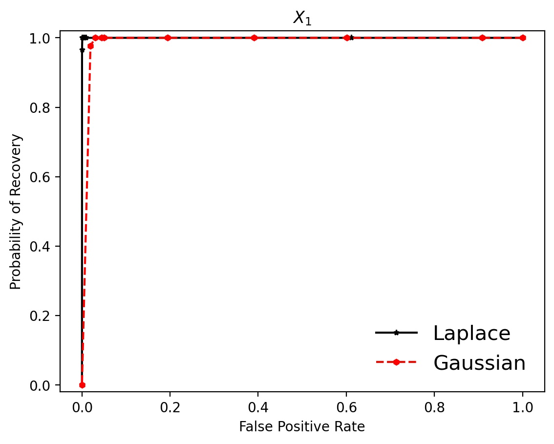
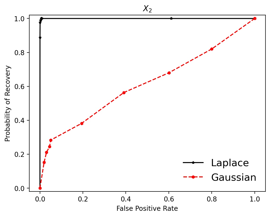
Figure 1. Probability of recovering a true variable against the false positive rate in the main effect model $Y=X_{1}+(X_{2}^{2}-1)+\mathsf{N}(0,\sigma^{2})$. Here $\sigma^{2}=4$, $n=p=1000$ and $\lambda=0.01$. To generate the ROC curve, $\gamma$ is varied over a grid of values: $(0,0.002,0.005,0.01,0.02,0.05,0.20,0.6,2.0)$.

6.2. Recovery of signals

We investigate the power of the algorithm in recovering main effects and hierarchical interactions. We generate the data according to

$$Y=X_{1}+X_{1}X_{2}+X_{1}X_{2}X_{3}+\mathsf{N}(0,\sigma^{2})~{}~{}\text{where}~{}~{}X\sim\mathsf{N}(0,I_{p}).$$

The variable $X_{1}$ is a main effect signal. The variables $X_{2},X_{3}$ are level $2$ and $3$ signals respectively. For this experiment, we use an $\ell_{1}$ kernel.

Figure 2 shows that the algorithm is able to detect high-order hierarchical interactions, though its power to detect interactions decreases as the level of the interaction increases.

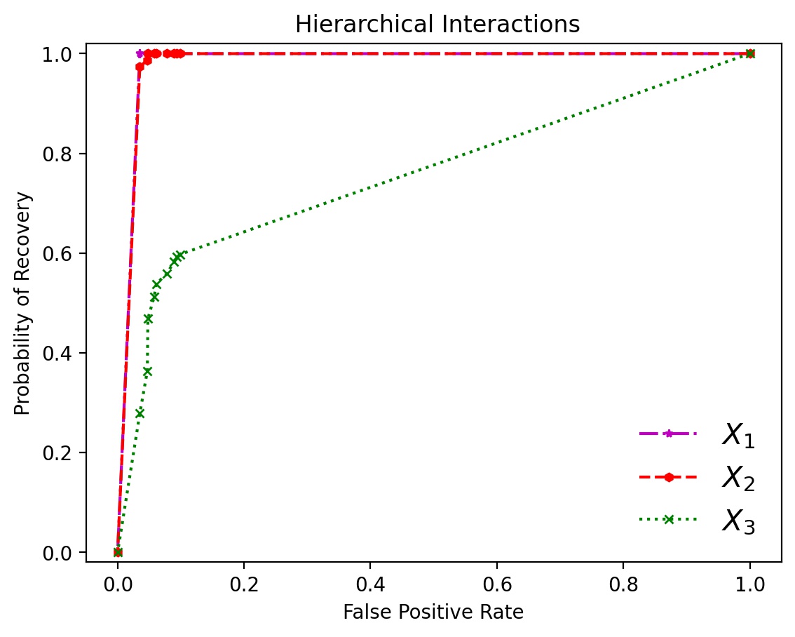
Figure 2. Probability of recovery of true variables against the false positive rate in the hierarchical interaction model $Y=X_{1}+X_{1}X_{2}+X_{1}X_{2}X_{3}+\mathsf{N}(0,\sigma^{2})$. Here $\sigma^{2}=1$, $n=p=1000$ and $\lambda=0.01$. To generate the ROC curve, $\gamma$ is varied over a grid of values: $(0,0.002,0.005,0.01,0.02,0.05,0.2,0.5,1.0)$.

7. Discussion

While kernel feature selection is a standard methodology for variable selection in nonparametric statistics—one which has been deployed in numerous applied problems—there has been little statistical theory to support the methodology. A core challenge is that the methodology is based on a nonconvex optimization problem. Progress has been made in studying the statistical properties of the global minima of the objective function, but there is a mismatch between such analyses and practice, given that the gradient-based methods available for high-dimensional nonconvex optimization are only able to find local minima.

We have accordingly studied the landscape associated with kernel feature selection, focusing on its local minima. We have shown that the design of the kernel is crucial if methods that find local minima are to succeed in the task of feature selection. In particular, we have shown that the choice of $\ell_{1}$ kernel eliminates bad stationary points that may trap gradient descent. We have established this result via the development of novel techniques that may have applications to a range of other kernel-based algorithms.

Appendix A A Roadmap to the Appendix

• Section B sets up the basics of kernel ridge regressions.

• Section C computes the gradient $\nabla\mathcal{J}(\beta)$.

• Section D shows the gradient $\nabla\mathcal{J}(\beta)$ is Lipschitz and uniformly bonded.

• Section E establishes the landscape result in Section 3 of the main text.

• Section F establishes the population-level guarantees of the kernel feature selection.

• Section G proves concentration results in the main text.

• Section H establishes the finite-sample guarantees of the kernel feature selection.

• Section I shows that—in a broader situation than considered in the main text—kernel feature selection is able to recover the Markov blanket.

• Section J proves the results in Section 2 of the main text.

• Section K gives basics on RKHS, functional analysis, concentration and optimization.

Appendix B Preliminaries

This section establishes the foundational properties of the family of kernel ridge regressions considered in the main text (with parameter $\beta$).

$$\begin{split}{\rm KRR}(\beta):~{}\mathop{\rm minimize}_{f\in\mathcal{H}}~{}~{}~{}&\mathcal{E}(\beta,f)\\ ~{}~{}\text{where}~{}~{}~{}~{}&\mathcal{E}(\beta,f)=\frac{1}{2}\mathbb{E}[(Y-f(\beta^{1/q}\odot X))^{2}]+\frac{\lambda}{2}\left\|{f}\right\|_{\mathcal{H}}^{2}.\end{split}$$ (B.1)

Let $f_{\beta}$ denote the minimizer and $\mathcal{J}(\beta)$ denote the minimum value of ${\rm KRR}(\beta)$.

• We characterize $f_{\beta}$ and $\mathcal{J}(\beta)$ using tools from functional analysis [FBJ04, FBJ09].

• We prove bounds on the solution $f_{\beta}$ and on the residual $r_{\beta}$.

• We prove continuity of the mapping $\beta\mapsto f_{\beta}$, $\beta\mapsto r_{\beta}$ and $\beta\mapsto\mathcal{J}(\beta)$.

B.1. Characterization of $f_{\beta}$ and $\mathcal{J}(\beta)$

Recall the following definitions (Definition 5.1).

• For each $\beta\geq 0$, the cross covariance operator $\Sigma_{\beta}:\mathcal{H}\mapsto\mathcal{H}$ is the mapping

  $$(\Sigma_{\beta}f)(\cdot)=\mathbb{E}\left[k(\beta^{1/q}\odot X,\cdot)f(\beta^{1/q}\odot X)\right].$$

• For each $\beta\geq 0$, the covariance function $h_{\beta}\in\mathcal{H}$ is $h_{\beta}(\cdot)=\mathbb{E}[k(\beta^{1/q}\odot X,\cdot)Y]$.

Proposition 8 characterizes the minimum $f_{\beta}$ and the minimum value $\mathcal{J}_{\beta}$ of ${\rm KRR}(\beta)$.

Proposition 8.

The minimum solution $f_{\beta}$ of the problem ${\rm KRR}(\beta)$ can be represented by

$$f_{\beta}=(\Sigma_{\beta}+\lambda I)^{-1}h_{\beta}.$$ (B.2)

The minimum value $\mathcal{J}(\beta)$ of the problem ${\rm KRR}(\beta)$ can be written as

$$\mathcal{J}(\beta)=\frac{1}{2}\mathbb{E}[Y^{2}]-\langle h_{\beta},(\Sigma_{\beta}+\lambda I)^{-1}h_{\beta}\rangle_{\mathcal{H}}.$$ (B.3)

Proof    By the reproducing property of the kernel $(x,x^{\prime})\mapsto k(x,x^{\prime})$, we have for any $f\in\mathcal{H}$ $\langle\Sigma_{\beta}f,f\rangle_{\mathcal{H}}=\mathbb{E}[f(\beta^{1/q}\odot X)^{2}]$, and $\langle h_{\beta},f\rangle_{\mathcal{H}}=\mathbb{E}[f(\beta^{1/q}\odot X)Y]$. Hence we can re-write the objective into $\mathcal{E}(\beta,f)=\frac{1}{2}\langle(\Sigma_{\beta}+\lambda I)f,f\rangle_{\mathcal{H}}-\langle h_{\beta},f\rangle_{\mathcal{H}}+\frac{1}{2}\mathbb{E}[Y^{2}]$. Note that $f\mapsto\mathcal{E}(\beta,f)$ is strongly convex w.r.t $\left\|{\cdot}\right\|_{\mathcal{H}}$ topology as $\Sigma_{\beta}$ is non-negative on $\mathcal{H}$. Hence the minimum $f_{\beta}$ is unique, and satisfies $(\Sigma_{\beta}+\lambda I)f=h_{\beta}$, i.e., equation (B.2). Formula (B.3) now follows.

∎

Proposition 9 (Variational Representation).

The following holds for any $g\in\mathcal{H}$:

$$\mathbb{E}[r_{\beta}(\beta^{1/q}\odot X;Y)g(\beta^{1/q}\odot X)]=\lambda\langle f_{\beta},g\rangle_{\mathcal{H}}.$$ (B.4)

Proof    The result follows by taking a first variation of the functional $f\mapsto\mathcal{E}(\beta,f)$. ∎

B.2. Bounds on $f_{\beta}$ and $r_{\beta}$

We bound the second moments of $f_{\beta}$ and $r_{\beta}$.

Proposition 10.

The solution $f_{\beta}$ and the residual $r_{\beta}$ satisfy

$$\big{\|}{f_{\beta}(\beta^{1/q}\odot X)}\big{\|}_{\mathcal{L}_{2}(\mathbb{P})}\leq\left\|{Y}\right\|_{\mathcal{L}_{2}(\mathbb{P})},~{}~{}~{}\big{\|}{r_{\beta}(\beta^{1/q}\odot X;Y)}\big{\|}_{\mathcal{L}_{2}(\mathbb{P})}\leq\left\|{Y}\right\|_{\mathcal{L}_{2}(\mathbb{P})}.$$

Proof    By Proposition 9, we get $\mathbb{E}[r_{\beta}(\beta^{1/q}\odot X;Y)f_{\beta}(\beta^{1/q}\odot X)]=\lambda\left\|{f_{\beta}}\right\|^{2}\geq 0$. Note then $r_{\beta}(\beta^{1/q}\odot x;y)=y-f_{\beta}(\beta^{1/q}\odot x)$ by definition. Hence, we obtain

$$\big{\|}{f_{\beta}(\beta^{1/q}\odot X)}\big{\|}_{\mathcal{L}_{2}(\mathbb{P})}^{2}\leq\mathbb{E}[Yf_{\beta}(\beta^{1/q}\odot X)]\leq\big{\|}{Y}\big{\|}_{\mathcal{L}_{2}(\mathbb{P})}\big{\|}{f_{\beta}(\beta^{1/q}\odot X)}\big{\|}_{\mathcal{L}_{2}(\mathbb{P})}.$$

This proves the first bound. The second bound can be deduced similarly. ∎

B.3. Continuity of the Mappings: $\beta\mapsto f_{\beta}$, $\beta\mapsto r_{\beta}$ and $\beta\mapsto\mathcal{J}(\beta)$.

Proposition 11.

We have the following results.

1. The mapping $\beta\mapsto f_{\beta}$ is continuous w.r.t the norm topology in $\mathcal{H}$, i.e.,

   $$\lim_{\beta^{\prime}\to\beta}\left\|{f_{\beta^{\prime}}-f_{\beta}}\right\|_{\mathcal{H}}=0$$

2. The mapping $\beta\mapsto f_{\beta}$ and $\beta\mapsto r_{\beta}$ is continuous w.r.t the sup norm $\left\|{\cdot}\right\|_{\infty}$:

   $$\lim_{\beta^{\prime}\to\beta}\left\|{f_{\beta^{\prime}}-f_{\beta}}\right\|_{\infty}=\lim_{\beta^{\prime}\to\beta}\left\|{r_{\beta^{\prime}}-r_{\beta}}\right\|_{\infty}=0$$

3. The mapping $\beta\mapsto\mathcal{J}(\beta)$ is continuous.

Proof    The key to the proof is to show that $\beta\mapsto h_{\beta}$ and $\beta\mapsto\Sigma_{\beta}$ are continuous

$$\lim_{\beta^{\prime}\to\beta}\left\|{h_{\beta^{\prime}}-h_{\beta}}\right\|_{\mathcal{H}}=0~{}~{}\text{and}~{}~{}\lim_{\beta^{\prime}\to\beta}\left|\!\left|\!\left|{\Sigma_{\beta^{\prime}}-\Sigma_{\beta}}\right|\!\right|\!\right|_{\rm op}=0.$$ (B.5)

Deferring its proof to the end, we first show why Proposition 11 follows from equation (B.5).

1. By Proposition 8, $f_{\beta}=(\Sigma_{\beta}+\lambda I)^{-1}h_{\beta}$. Hence, the mapping $\beta\mapsto f_{\beta}$ is contiuous w.r.t the norm topology in $\mathcal{H}$ since $\beta\mapsto h_{\beta}$ and $\beta\mapsto\Sigma_{\beta}$ are continuous by equation (B.5).

2. Note that $\left\|{g}\right\|_{\infty}\leq|h(0)|^{1/2}\left\|{g}\right\|_{\mathcal{H}}$ for any $g\in\mathcal{H}$. Indeed, by reproducing property of $\mathcal{H}$:

   $$\left\|{g}\right\|_{\infty}=\sup_{x}|g(x)|=\sup_{x}|\langle k(x,\cdot),g\rangle_{\mathcal{H}}|\leq\sup_{x}k(x,x)^{1/2}\left\|{g}\right\|_{\mathcal{H}}\leq|h(0)|^{1/2}\left\|{g}\right\|_{\mathcal{H}}.$$

   Hence $\lim_{\beta^{\prime}\to\beta}\left\|{f_{\beta^{\prime}}-f_{\beta}}\right\|_{\infty}=0$ as a consequence of part (a). Note $r_{\beta}-r_{\beta^{\prime}}=f_{\beta^{\prime}}-f_{\beta}$.

3. By Proposition 8, $\mathcal{J}(\beta)=\frac{1}{2}\mathbb{E}[Y^{2}]-\langle h_{\beta},(\Sigma_{\beta}+\lambda I)^{-1}h_{\beta}\rangle_{\mathcal{H}}$. The continuity of $\beta\mapsto\mathcal{J}(\beta)$ follows easily as a consequence of the fact that both $\beta\mapsto h_{\beta}$ and $\beta\mapsto\Sigma_{\beta}$ are continuous.

It remains to prove equation (B.5). The key is to notice the identities below (similar ones appear in the literature [FBJ04, GBSS05]): letting $(X^{\prime},Y^{\prime})$ be independent copies of $(X,Y)$,

$$\left\|{h_{\beta^{\prime}}-h_{\beta}}\right\|_{\mathcal{H}}^{2} =\mathbb{E}[(k(\beta^{1/q}\odot X,\beta^{1/q}\odot X^{\prime})+k(\beta^{\prime 1/q}\odot X,\beta^{\prime 1/q}\odot X^{\prime})-2k(\beta^{1/q}\odot X,\beta^{\prime 1/q}\odot X^{\prime}))YY^{\prime}]$$

$$\left\|{\Sigma_{\beta^{\prime}}-\Sigma_{\beta}}\right\|_{{\rm HS}}^{2} =\mathbb{E}[k(\beta^{1/q}\odot X,\beta^{1/q}\odot X^{\prime})^{2}+k(\beta^{\prime 1/q}\odot X,\beta^{\prime 1/q}\odot X^{\prime})^{2}-2k(\beta^{1/q}\odot X,\beta^{\prime 1/q}\odot X^{\prime})^{2}]$$

Note also $\left|\!\left|\!\left|{\Sigma}\right|\!\right|\!\right|_{\rm op}\leq\left\|{\Sigma}\right\|_{{\rm HS}}$ for any operator $\Sigma$. As a result, equation (B.5) follows from the above identities and the fact that $(x,x^{\prime})\mapsto k(x,x^{\prime})$ is continuous and uniformly bounded. ∎

Proposition 12.

The mapping $\beta\mapsto r_{\beta}(\beta^{1/q}\odot\cdot;\cdot)$ is continuous w.r.t the norm $\left\|{\cdot}\right\|_{\mathcal{L}_{2}(\mathbb{P})}$:

$$\lim_{\beta^{\prime}\mapsto\beta}\big{\|}{r_{\beta}(\beta^{1/q}\odot X;Y)-r_{\beta^{\prime}}(\beta^{\prime 1/q}\odot X;Y)}\big{\|}_{\mathcal{L}_{2}(\mathbb{P})}=0.$$

Proof    It suffices to prove that $\beta\mapsto f_{\beta}(\beta^{1/q}\odot\cdot)$ is continuous w.r.t $\left\|{\cdot}\right\|_{\infty}$ topology. This is true since (i) $f_{\beta}(\beta^{1/q}\odot x)=\langle f_{\beta},k(\beta^{1/q}\odot x,\cdot)\rangle_{\mathcal{H}}$, $(ii)$ $\beta\mapsto f_{\beta}$ is continuous w.r.t $\left\|{\cdot}\right\|_{\mathcal{H}}$, and $(iii)$ $\beta\mapsto k(\beta^{1/q}\odot x,\cdot)$ is uniformly (uniform w.r.t $x$) continuous w.r.t $\left\|{\cdot}\right\|_{\mathcal{H}}$ topology. ∎

Appendix C Computation of the Gradient $\nabla\mathcal{J}(\beta)$: Proof of Proposition 4

This section substantiates the proof of Proposition 4 in the main text.

C.1. Notation.

Recall the objective function

$$\mathcal{E}(\beta,f)=\frac{1}{2}~{}\mathbb{E}[(Y-f(\beta^{1/q}\odot X))^{2}]+\frac{\lambda}{2}\left\|{f}\right\|_{\mathcal{H}}^{2}.$$

To facilitate the proof, we perform a change of variable. Introduce the auxiliary objective

$$\begin{split}\widetilde{\mathcal{E}}(\beta,f)&=\frac{1}{2}~{}\mathbb{E}[(Y-f(X))^{2}]+\frac{\lambda}{2}\left\|{f}\right\|_{\mathcal{H}_{\beta}}^{2},\\ &=\frac{1}{2}\mathbb{E}[(Y-f(X))^{2}]+\frac{\lambda}{2(2\pi)^{p}}\int|\mathcal{F}(f)(\omega)|^{2}\cdot\frac{1}{Q_{\beta}(\omega)}d\omega\end{split}$$ (C.1)

where $\mathcal{H}_{\beta}$ is the RKHS with kernel $(x,x^{\prime})\mapsto k(\beta^{1/q}\odot x;\beta^{1/q}\odot x^{\prime})$ (Section C.8 gives details on the construction of $\mathcal{H}_{\beta}$). A simple consequence of Proposition 13 yields for $\beta>0$

$$\mathcal{J}(\beta)=\min_{f\in\mathcal{H}}\mathcal{E}(\beta,f)=\min_{f\in\mathcal{H}_{\beta}}\widetilde{\mathcal{E}}(\beta,f).$$ (C.2)

Let $\widetilde{f}_{\beta}\in\mathcal{H}_{\beta}$ denote the minimum of $f\mapsto\widetilde{\mathcal{E}}(\beta,f)$ so that $J(\beta)=\widetilde{\mathcal{E}}(\beta,\widetilde{f}_{\beta})$.

C.2. Main Proof.

Lemma C.1 gives an initial analytic representation of $\nabla\mathcal{J}(\beta)$.

Lemma C.1.

For any $\beta>0$, $\nabla\mathcal{J}(\beta)$ exists, and satisfies

$$\nabla\mathcal{J}(\beta)=\frac{\lambda}{(2\pi)^{p}}\cdot\int|\mathcal{F}(\widetilde{f}_{\beta})(\omega)|^{2}\cdot\nabla_{\beta}\left(\frac{1}{Q_{\beta}(\omega)}\right)d\omega.$$ (C.3)

As explained in the main text, in order for one to apply the “envelope theorem” to the variational formula $\mathcal{J}(\beta)=\min_{f\in\mathcal{H}_{\beta}}\widetilde{\mathcal{E}}(\beta,f)$. one needs to establish that the solution $\widetilde{f}_{\beta}$ is a sufficiently smooth function (e.g., it is sufficiently smooth so that the RHS of equation (C.3) exists). To achieve this goal, Lemma C.2 is crucial. Write $\widetilde{r}_{\beta}(x;y)=y-\widetilde{f}_{\beta}(x)$.

Lemma C.2.

Let $\beta>0$. The identity below holds for almost all $\omega$ (w.r.t Lebesgue measure)

$$\frac{1}{(2\pi)^{p/2}}\cdot\mathcal{F}(\widetilde{f}_{\beta})(\omega)=\frac{1}{\lambda}\cdot\mathbb{E}\left[\widetilde{r}_{\beta}(X;Y)e^{i\langle\omega,X\rangle}\right]\cdot Q_{\beta}(\omega).$$ (C.4)

Equivalently, the following identity holds for almost all $\omega$ (w.r.t Lebesgue measure)

$$\frac{1}{(2\pi)^{p/2}}\cdot\mathcal{F}(f_{\beta})(\omega)=\frac{1}{\lambda}\cdot\mathbb{E}\left[r_{\beta}(\beta^{1/q}\odot X;Y)e^{i\langle\omega,\beta^{1/q}\odot X\rangle}\right]\cdot Q(\omega).$$ (C.5)

Remark     The main idea to prove Lemma C.2 is to use the characterization of $\widetilde{f}_{\beta}$:

$$\mathbb{E}[\widetilde{r}_{\beta}(X;Y)\widetilde{g}(X)]=\lambda\langle\widetilde{f}_{\beta},\widetilde{g}\rangle_{\mathcal{H}_{\beta}}~{}~{}\text{for all $g\in\mathcal{H}_{\beta}$}$$

which can be derived by taking the first order variation of the objective $f\mapsto\widetilde{\mathcal{E}}(\beta,f)$. We then wish to substitute $\widetilde{g}(x)=e^{i\omega^{T}x}$ and obtain Lemma C.2. The challenge that remains is that the complex basis function $x\mapsto e^{i\omega^{T}x}$ does not belong to $\mathcal{H}_{\beta}$. As a result, we apply the mollifier trick—common in harmonic analysis—to overcome this technical issue.

Back to the proof of Proposition 4. By Lemma C.1 and Lemma C.2, we obtain for $\beta>0$

$$\begin{split}\nabla\mathcal{J}(\beta)&=\frac{\lambda}{(2\pi)^{p}}\int|\mathcal{F}(\widetilde{f}_{\beta})(\omega)|^{2}\cdot\nabla_{\beta}\left(\frac{1}{Q_{\beta}(\omega)}\right)d\omega.\\ &=-\frac{1}{\lambda}\cdot\int\left|\mathbb{E}[\widetilde{r}_{\beta}(X;Y)e^{i\omega^{T}X}]\right|^{2}\cdot\nabla_{\beta}Q_{\beta}(\omega)d\omega\\ &=-\frac{1}{\lambda}\cdot\mathbb{E}\left[\widetilde{r}_{\beta}(X;Y)\widetilde{r}_{\beta}(X^{\prime};Y^{\prime})\int e^{i\langle\omega,X-X^{\prime}\rangle}\cdot\nabla_{\beta}Q_{\beta}(\omega)d\omega\right]\end{split}$$ (C.6)

The next lemma evaluates the integral inside the expectation.

Lemma C.3.

For all $\beta>0$, we have the identity that holds for $l\in[p]$:

$$h^{\prime}(\left\|{X-X^{\prime}}\right\|_{q,\beta}^{q})\cdot|X_{l}-X_{l}^{\prime}|^{q}=\int e^{i\langle\omega,X-X^{\prime}\rangle}\cdot(\partial_{\beta_{l}}Q_{\beta}(\omega))d\omega.$$

By Lemma C.3 and equation (C.6), we obtain for all $\beta>0$ and $l\in[p]$

$$\begin{split}(\nabla\mathcal{J}(\beta))_{l}&=-\frac{1}{\lambda}\cdot\mathbb{E}\left[\widetilde{r}_{\beta}(X;Y)\widetilde{r}_{\beta}(X^{\prime};Y^{\prime})h^{\prime}(\left\|{X-X^{\prime}}\right\|_{q,\beta}^{q})|X_{l}-X_{l}^{\prime}|^{q}\right]\\ &=-\frac{1}{\lambda}\cdot\mathbb{E}\left[r_{\beta}(\beta^{1/q}\odot X;Y)r_{\beta}(\beta^{1/q}\odot X^{\prime};Y^{\prime})h^{\prime}(\left\|{X-X^{\prime}}\right\|_{q,\beta}^{q})|X_{l}-X_{l}^{\prime}|^{q}\right].\end{split}$$ (C.7)

To extend the result from positive $\beta>0$ to non-negative $\beta\geq 0$, we use Lemma C.4.

Lemma C.4.

Let $F:\mathbb{R}_{+}\mapsto\mathbb{R}$ be continuous. Suppose $F$ is differentiable on $x>0$, and $\lim_{x\to 0^{+}}F^{\prime}(x)$ exists. Then, $F^{\prime}_{+}(0)$ exists and $F^{\prime}_{+}(0)=\lim_{x\to 0^{+}}F^{\prime}(x)$.

Recall that $\beta\mapsto\mathcal{J}(\beta)$ is continuous for $\beta\geq 0$ (Proposition 11). Also, the mapping

$$\beta\mapsto-\frac{1}{\lambda}\cdot\mathbb{E}\left[r_{\beta}(\beta^{1/q}\odot X;Y)r_{\beta}(\beta^{1/q}\odot X^{\prime};Y^{\prime})h^{\prime}(\left\|{X-X^{\prime}}\right\|_{q,\beta}^{q})|X_{l}-X_{l}^{\prime}|^{q}\right]$$

is continuous for $\beta\geq 0$ (Proposition 10 and 12). Hence, equation (C.7) holds for all $\beta\geq 0$.

C.3. Proof of Lemma C.2.

It suffices to prove equation (C.4). Note that equation (C.5) follows by a change of variable (by substituting $\beta^{1/q}\odot\omega$ into $\omega$ in equation (C.4)).

Below we prove equation (C.4). By taking the first order variation of $f\mapsto\widetilde{\mathcal{E}}(\beta,f)$, we obtain the following characterization of $\widetilde{f}_{\beta}$: for all $\widetilde{g}\in\mathcal{H}_{\beta}$

$$\mathbb{E}[\widetilde{r}_{\beta}(X;Y)\widetilde{g}(X)]=\lambda\langle\widetilde{f}_{\beta},\widetilde{g}\rangle_{\mathcal{H}_{\beta}}.$$ (C.8)

As a result, using Corollary C.1 to expand the RHS, this proves that for all functions $\widetilde{g}\in\mathcal{H}_{\beta}$:

$$\mathbb{E}[\widetilde{r}_{\beta}(X;Y)\widetilde{g}(X)]=\frac{\lambda}{(2\pi)^{p}}\int\frac{\mathcal{F}(\widetilde{f}_{\beta})(\omega^{\prime})\mathcal{F}(\widetilde{g})(\omega^{\prime})}{Q_{\beta}(\omega^{\prime})}d\omega^{\prime}.$$ (C.9)

To motivate the rest of the proof, we first give a quick heuristic derivation of Lemma C.2. Let $\widetilde{g}_{\omega}(x)=e^{i\omega^{T}x}$. The idea is to substitute $\widetilde{g}=\widetilde{g}_{\omega}$ into equation (C.9). To compute the RHS, $\mathcal{F}(\widetilde{g}_{\omega})(\cdot)=(2\pi)^{p/2}\delta_{\omega}(\cdot)$ where $\delta_{\omega}$ is the $\delta$-function centered at $\omega$. This gives

$$\mathbb{E}\left[\widetilde{r}_{\beta}(X;Y)e^{i\omega^{T}x}\right]=\frac{\lambda}{(2\pi)^{p}}\int\frac{\mathcal{F}(\widetilde{f}_{\beta})(\omega^{\prime})\mathcal{F}(\widetilde{g}_{\omega})(\omega^{\prime})}{Q_{\beta}(\omega^{\prime})}d\omega^{\prime}=\frac{\lambda}{(2\pi)^{p/2}}\cdot\frac{\mathcal{F}(\widetilde{f}_{\beta})(\omega)}{Q_{\beta}(\omega)}.$$

Of course, the above derivation is not rigorous. The function $\widetilde{g}_{\omega}(x)=e^{i\omega^{T}x}$ lacks regularity and does not belong to $\mathcal{H}_{\beta}$. To obtain a rigorous treatment, we need to smooth $\widetilde{g}_{\omega}$ and borrow the regularity $\mathbb{E}[Y^{2}]<\infty$ to overcome this technical issue.

Below is the rigorous derivation. Define, for any $\epsilon>0$, the function $\widetilde{g}_{\omega,\epsilon}$ by

$$\widetilde{g}_{\omega,\epsilon}(x)=\widetilde{g}_{\omega}(x)\cdot k_{\epsilon}(x)~{}~{}\text{where $k_{\epsilon}(x)=k(\epsilon x)$ for $k(x)=\prod_{i=1}^{p}(\sin(x_{i})/x_{i})$}.$$

Note that (i) $\mathcal{F}(k)$ is compactly supported (ii) $k$ is uniformly bounded: $\sup_{x}|k(x)|<\infty$. Since $\mathcal{F}(k)$ is compactly supported, $\widetilde{g}_{\omega,\epsilon}\in\mathcal{H}_{\beta}$ for any $\epsilon>0$ by Corollary C.1. Additionally,

$$\mathcal{F}(\widetilde{g}_{\omega,\epsilon})(\cdot)=\mathcal{F}(k_{\epsilon})(\cdot-\omega)~{}~{}\text{where $\mathcal{F}(k_{\epsilon})(\omega^{\prime})=(2\pi)^{p/2}\cdot\prod_{i=1}^{p}(\mathbf{1}_{w_{i}^{\prime}\in[-\epsilon,\epsilon]}/(2\epsilon))$}.$$

Substitute $\widetilde{g}_{\omega,\epsilon}$ into $\widetilde{g}$ in equation (C.9). This yields the identity that holds for all $\epsilon>0$

$$\begin{split}\mathbb{E}[\widetilde{r}_{\beta}(X;Y)e^{i\omega^{T}X}k_{\epsilon}(X)]&=\frac{\lambda}{(2\pi)^{p}}\cdot\left(\bigg{(}\frac{\mathcal{F}(\widetilde{f}_{\beta})}{Q_{\beta}}\bigg{)}*\mathcal{F}(k_{\epsilon})\right)(\omega).\end{split}$$ (C.10)

Now we take $\epsilon\to 0^{+}$ on both sides. We shall show that will yield Lemma C.2.

1. Take the limit $\epsilon\to 0^{+}$ on the LHS of equation (C.10):

   $$\lim_{\epsilon\to 0^{+}}\mathbb{E}\left[\widetilde{r}_{\beta}(X;Y)e^{i\omega^{T}X}k_{\epsilon}(X)\right]=\mathbb{E}\left[\widetilde{r}_{\beta}(X;Y)e^{i\omega^{T}X}\right].$$

   This follows from the dominated convergence theorem: (i) $\lim_{\epsilon\to 0^{+}}k_{\epsilon}(x)=1$ (ii) $\mathbb{E}[|[\widetilde{r}_{\beta}(X;Y)|]\leq(\mathbb{E}[Y^{2}])^{1/2}<\infty$ by Proposition 10 and (iii) $\sup_{x}|k_{\epsilon}(x)|=\sup_{x}|k(x)|<\infty$.

2. Take the limit $\epsilon\to 0^{+}$ on the RHS of equation (C.10):

   $$\lim_{\epsilon\to 0^{+}}\left(\bigg{(}\frac{\mathcal{F}(\widetilde{f}_{\beta})}{Q_{\beta}}\bigg{)}*\mathcal{F}(k_{\epsilon})\right)(\omega)\to(2\pi)^{p/2}\cdot\frac{\mathcal{F}(\widetilde{f}_{\beta})}{Q_{\beta}}(\omega)~{}~{}\text{a.e.-$\omega$}.$$ (C.11)

   This follows by applying Lebesgue’s almost-everywhere differentiable theorem to the locally integrable function $\omega\mapsto\frac{\mathcal{F}(\widetilde{f}_{\beta})}{Q_{\beta}}$. To see why it is locally integrable, we note that: (i) the function $\omega\mapsto Q_{\beta}(\omega)$ is positive and continuous (ii) $\mathcal{F}(f_{\beta})$ is integrable since

   $$\begin{split}\left(\int|\mathcal{F}(\widetilde{f}_{\beta}(\omega))|d\omega\right)^{2}&\leq\int\frac{|\mathcal{F}(\widetilde{f}_{\beta}(\omega))|^{2}}{Q_{\beta}(\omega)}d\omega\cdot\int Q_{\beta}(\omega)d\omega=(2\pi)^{p}|h(0)|\big{\|}{\widetilde{f}_{\beta}}\big{\|}_{\mathcal{H}}^{2}<\infty.\end{split}$$

C.4. Proof of Lemma C.3.

Our starting point is the following identity: for any $\beta>0$

$$h(\left\|{x-x^{\prime}}\right\|_{q,\beta}^{q})=\int e^{i\langle\omega,\beta^{1/q}\odot(x-x^{\prime})\rangle}Q(\omega)d\omega=\int e^{i\langle\omega,x-x^{\prime}\rangle}Q_{\beta}(\omega)d\omega.$$

Take partial derivative $\partial_{\beta_{l}}$ on both sides. We wish to apply Lebesgue’s dominated convergence theorem to exchange the integral and the derivative operations. This requires a careful check of regularity conditions. We divide our discussions based on the value of $q$.

• Case $q=1$. In this case,one can show that the following bound holds for all $\omega$:

  $$|\partial_{\beta_{l}}Q_{\beta}(\omega)|\leq\frac{1}{\beta_{l}}|Q_{\beta}(\omega)|.$$

  Note that $\sup_{\beta\in B}Q_{\beta}(\omega)(1+\omega_{l}^{2})$ is integrable for compact $B$ which does not contain $0$.

• Case $q=2$. In this case, we assume $\mathop{\rm supp}(\mu)$ is away from $0$: say for some $m_{\mu}>0$, we have $\mathop{\rm supp}(\mu)\subseteq[m_{\mu},\infty)$. One can then show the following bound which holds for all $\omega$:

  $$|\partial_{\beta_{l}}Q_{\beta}(\omega)|\leq\frac{1}{(1\wedge\beta_{l})^{2}\cdot(1\wedge m_{\mu})}|Q_{\beta}(\omega)|(1+\omega_{l}^{2}).$$

  Note that $\sup_{\beta\in B}Q_{\beta}(\omega)(1+\omega_{l}^{2})$ is integrable for compact $B$ which does not contain $0$.

Let $\beta>0$ and $B$ be any compact set which does not contain $0$. We conclude for $q=1,2$

$$\int\sup_{\beta\in B}|\partial_{\beta_{l}}Q_{\beta}(\omega)|d\omega<\infty.$$

As a result, the dominated convergence theorem implies the desired identity:

$$\begin{split}h^{\prime}(\langle\beta,|x-x^{\prime}|\rangle)|x_{l}-x_{l}^{\prime}|^{q}&=\partial_{\beta_{l}}\left(\int e^{i\langle\omega,x-x^{\prime}\rangle}Q_{\beta}(\omega)d\omega\right)=\int e^{i\langle\omega,x-x^{\prime}\rangle}\cdot(\partial_{\beta_{l}}Q_{\beta}(\omega))d\omega.\end{split}$$

C.5. Proof of Lemma C.1.

For any $f$, let $\nabla_{\beta}\widetilde{\mathcal{E}}(\beta,f)$ denote the gradient of $\widetilde{\mathcal{E}}(\beta,f)$ with respect to $\beta$ at $f$ (if it exists). We prove the following result (proof in Section C.6).

Lemma C.5.

Fix $\beta>0$. Then we have the following statements.

1. Existence: $\nabla_{\beta}\widetilde{\mathcal{E}}(\beta{{}^{\prime\prime}},f_{\beta^{\prime}})$ exists for all $\beta^{\prime},\beta^{\prime\prime}$ in a neighborhood of $\beta$.

2. Continuity: $\nabla_{\beta}\widetilde{\mathcal{E}}(\beta{{}^{\prime\prime}},f_{\beta^{\prime}})\to\nabla_{\beta}\widetilde{\mathcal{E}}(\beta,f_{\beta})$ as $\beta^{\prime},\beta^{\prime\prime}\to\beta$.

3. Analytical expression: for all $\beta^{\prime},\beta^{\prime\prime}$ close to $\beta$, we have

   $$\nabla_{\beta}\widetilde{\mathcal{E}}(\beta^{\prime},f_{\beta^{\prime\prime}})=\frac{\lambda}{(2\pi)^{p}}\int\Big{|}\mathcal{F}(\widetilde{f_{\beta^{\prime\prime}}})(\omega)\Big{|}^{2}\cdot\nabla_{\beta}\left(\frac{1}{Q_{\beta^{\prime}}(\omega)}\right)d\omega.$$ (C.12)

We are now ready to prove Lemma C.1. We first prove that

$$\mathcal{J}(\beta^{\prime})\geq\mathcal{J}(\beta)+\langle\nabla_{\beta}\mathcal{E}(\beta,\widetilde{f_{\beta}}),\beta^{\prime}-\beta\rangle+o(\left\|{\beta^{\prime}-\beta}\right\|_{2}).$$ (C.13)

Indeed, note that $\mathcal{J}(\beta^{\prime})=\mathcal{E}(\beta^{\prime},\widetilde{f_{\beta^{\prime}}})$ and $\mathcal{E}(\beta,\widetilde{f_{\beta^{\prime}}})\geq\mathcal{J}(\beta)$. Using Lemma C.5, for $\beta^{\prime}$ close to $\beta$, Taylor’s intermediate theorem yields for some $\beta^{\prime\prime}\in[\beta,\beta^{\prime}]$:

$$\mathcal{J}(\beta^{\prime})=\mathcal{E}(\beta,\widetilde{f_{\beta^{\prime}}})+\langle\nabla_{\beta}\mathcal{E}(\beta^{\prime\prime},\widetilde{f_{\beta^{\prime}}}),\beta^{\prime}-\beta\rangle\geq\mathcal{J}(\beta)+\langle\nabla_{\beta}\mathcal{E}(\beta^{\prime\prime},\widetilde{f_{\beta^{\prime}}}),\beta^{\prime}-\beta\rangle.$$

Equation (C.13) now follows since $\nabla_{\beta}\mathcal{E}(\beta^{\prime\prime},\widetilde{f_{\beta^{\prime}}})\to\nabla_{\beta}\widetilde{\mathcal{E}}(\beta,f_{\beta})$ by Lemma C.5. With the same reasoning, one can analogously derive

$$\mathcal{J}(\beta^{\prime})\leq\mathcal{J}(\beta)+\langle\nabla_{\beta}\mathcal{E}(\beta,\widetilde{f_{\beta}}),\beta^{\prime}-\beta\rangle+o(\left\|{\beta^{\prime}-\beta}\right\|_{2}).$$ (C.14)

Equations (C.13) and (C.14) together yield the desired claim of Lemma C.1.

C.6. Proof of Lemma C.5.

Recall the objective function

$$\widetilde{\mathcal{E}}(\beta^{\prime\prime},\widetilde{f_{\beta}^{\prime}})=\frac{1}{2}\mathbb{E}[(Y-\widetilde{f_{\beta}^{\prime}}(X))^{2}]+\frac{\lambda}{2(2\pi)^{p}}\int\Big{|}\mathcal{F}(\widetilde{f}_{\beta^{\prime}})(\omega)\Big{|}^{2}\cdot\frac{1}{Q_{\beta^{\prime\prime}}(\omega)}d\omega,$$

We wish to take the derivative w.r.t $\beta$. Let $B=\prod_{j=1}^{p}[c_{1}\beta_{j},c_{2}\beta_{j}]$ where $c_{1}=0.99$, $c_{2}=1.01$. The key to the proof is to prove the technical result:

$$\int\sup_{\beta^{\prime}\in B,\beta^{\prime\prime}\in B}\Big{|}\mathcal{F}(\widetilde{f_{\beta^{\prime}}})(\omega)\Big{|}^{2}\cdot\left\|{\nabla_{\beta}\left(\frac{1}{Q_{\beta^{\prime\prime}}(\omega)}\right)}\right\|_{2}d\omega<\infty.$$ (C.15)

We defer the proof equation (C.15) to the end. Note then, given equation (C.15), Lebesgue’s dominated convergence theorem implies that $\nabla_{\beta}\widetilde{\mathcal{E}}(\beta^{\prime},f_{\beta^{\prime\prime}})$ exists and satisfies (C.12). To prove the remaining claim, $\nabla\widetilde{\mathcal{E}}(\beta^{\prime\prime},\widetilde{f_{\beta^{\prime}}})\to\nabla\widetilde{\mathcal{E}}(\beta,\widetilde{f_{\beta}})$ as $\beta^{\prime\prime},\beta^{\prime}\to\beta$, it suffices to show that

$$\limsup_{\beta^{\prime\prime},\beta^{\prime}\to\beta}\int\left\|{\Big{|}\mathcal{F}(\widetilde{f_{\beta^{\prime}}})(\omega)\Big{|}^{2}\cdot\nabla_{\beta}\left(\frac{1}{Q_{\beta^{\prime\prime}}(\omega)}\right)-\Big{|}\mathcal{F}(\widetilde{f_{\beta}})(\omega)\Big{|}^{2}\cdot\nabla_{\beta}\left(\frac{1}{Q_{\beta}(\omega)}\right)}\right\|_{2}d\omega=0.$$ (C.16)

Below we prove the deferred equations (C.15) and (C.16).

To prove equation (C.15), we introduce the function $\omega\mapsto g(\omega)$

$$g(\omega)=\sup_{\beta^{\prime\prime},\beta^{\prime}\in B}\bigg{\{}\bigg{\|}{\nabla_{\beta}\Big{(}\frac{1}{Q_{\beta^{\prime\prime}}(\omega)}\Big{)}}\bigg{\|}_{2}\cdot Q_{\beta^{\prime}}^{2}(\omega)\bigg{\}}.$$

Lemma C.6 shows that $g$ is integrable. Now that

$$\begin{split}\int\sup_{\beta^{\prime}\in B,\beta^{\prime\prime}\in B}&\Big{|}\mathcal{F}(\widetilde{f_{\beta^{\prime}}})(\omega)\Big{|}^{2}\cdot\big{\|}{\nabla_{\beta}\Big{(}\frac{1}{Q_{\beta^{\prime\prime}}(\omega)}\Big{)}}\big{\|}_{2}d\omega\leq\int\sup_{\beta^{\prime\prime}\in B}|\mathcal{F}(\widetilde{f}_{\beta^{\prime}})(\omega)|^{2}\cdot\frac{g(\omega)}{Q_{\beta^{\prime}}^{2}(\omega)}d\omega\\ &\stackrel{{\scriptstyle(i)}}{{=}}\frac{(2\pi)^{p}}{\lambda^{2}}\cdot\int\sup_{\beta^{\prime\prime}\in B}\left|\mathbb{E}[\widetilde{r}_{\beta^{\prime}}(X;Y)e^{i\omega^{T}X}]\right|^{2}\cdot g(\omega)d\omega\stackrel{{\scriptstyle(ii)}}{{\leq}}\frac{(2\pi)^{p}}{\lambda^{2}}\cdot\mathbb{E}\left[|Y|^{2}\right]\cdot\int|g(\omega)|d\omega<\infty.\end{split}$$

where (i) is due to Lemma C.2 and (ii) is due to Proposition 10. This proves equation (C.15).

To prove equation (C.16), we introduce the functions

$$h_{\beta^{\prime},\beta^{\prime\prime}}(\omega)=\nabla_{\beta}\left(\frac{1}{Q_{\beta^{\prime\prime}}(\omega)}\right)\cdot Q_{\beta^{\prime}}^{2}(\omega)~{}~{}\text{and}~{}~{}z_{\beta}(\omega)=\nabla Q_{\beta}(\omega).$$

Note that the following bound holds for all $\beta,\beta^{\prime},\beta^{\prime\prime}$:

$$\begin{split}&\int\left\|{\Big{|}\mathcal{F}(\widetilde{f_{\beta^{\prime}}})(\omega)\Big{|}^{2}\cdot\nabla_{\beta}\left(\frac{1}{Q_{\beta^{\prime\prime}}(\omega)}\right)-\Big{|}\mathcal{F}(\widetilde{f_{\beta}})(\omega)\Big{|}^{2}\cdot\nabla_{\beta}\left(\frac{1}{Q_{\beta}(\omega)}\right)}\right\|_{2}d\omega\\ &=\int\bigg{\|}{|\mathcal{F}(\widetilde{f}_{\beta^{\prime}})(\omega)|^{2}\cdot\frac{h_{\beta^{\prime},\beta^{\prime\prime}}(\omega)}{Q_{\beta^{\prime}}^{2}(\omega)}-|\mathcal{F}(\widetilde{f}_{\beta})(\omega)|^{2}\cdot\frac{z_{\beta}(\omega)}{Q_{\beta}^{2}(\omega)}}\bigg{\|}_{2}d\omega\\ &\stackrel{{\scriptstyle(i)}}{{=}}\frac{(2\pi)^{p}}{\lambda^{2}}\cdot\int\bigg{\|}{\left|\mathbb{E}[\widetilde{r}_{\beta^{\prime}}(X;Y)e^{i\omega^{T}X}]\right|^{2}h_{\beta^{\prime},\beta^{\prime\prime}}(\omega)-\left|\mathbb{E}[\widetilde{r}_{\beta}(X;Y)e^{i\omega^{T}X}]\right|^{2}z_{\beta}(\omega)}\bigg{\|}_{2}d\omega\\ &\stackrel{{\scriptstyle(ii)}}{{\leq}}\frac{(2\pi)^{p}}{\lambda^{2}}\cdot\left(\int\left\|{h_{\beta^{\prime},\beta^{\prime\prime}}(\omega)-z_{\beta}(\omega)}\right\|_{2}d\omega\cdot\mathbb{E}[Y^{2}]+\left|\mathbb{E}[(\widetilde{r_{\beta^{\prime}}}-\widetilde{r_{\beta}})(X;Y)]\right|\cdot\mathbb{E}[Y^{2}]^{1/2}\cdot\int\left\|{z_{\beta}(\omega)}\right\|_{2}d\omega\right).\end{split}$$

where $(i)$ is due to Lemma C.2 and (ii) is due to Cauchy-Schwartz. Note $\limsup_{\beta^{\prime}\to\beta}|\mathbb{E}[(\widetilde{r_{\beta^{\prime}}}-\widetilde{r_{\beta}})(X;Y)]|=0$ by Proposition 12, and $\limsup_{\beta^{\prime},\beta^{\prime\prime}\to\beta}\int\left\|{h_{\beta^{\prime},\beta^{\prime\prime}}(\omega)-z_{\beta}(\omega)}\right\|_{2}d\omega=0$ by Lemma C.6 and Lebesgue’s dominated convergence theorem. This proves equation (C.16).

C.7. An Integrability Result on $Q_{\beta}$.

Lemma C.6.

Let $\beta>0$. For $B=\prod_{j=1}^{p}[c_{1}\beta_{j},c_{2}\beta_{j}]$ where $c_{1}=0.99$, $c_{2}=1.01$, we have

$$\int\sup_{\beta^{\prime\prime},\beta^{\prime}\in B}\bigg{\{}\bigg{\|}{\nabla_{\beta}\Big{(}\frac{1}{Q_{\beta^{\prime\prime}}(\omega)}\Big{)}}\bigg{\|}_{2}\cdot Q_{\beta^{\prime}}^{2}(\omega)\bigg{\}}d\omega<\infty.$$

Proof    It suffices to show that for any $l\in[p]$:

$$\int\sup_{\beta^{\prime\prime},\beta^{\prime}\in B}\bigg{\{}|\partial_{\beta_{l}}Q_{\beta^{\prime\prime}}(\omega)|\cdot\frac{Q_{\beta^{\prime}}^{2}(\omega)}{Q_{\beta^{\prime\prime}}^{2}(\omega)}\bigg{\}}d\omega<\infty.$$

• Case $q=1$. In this case, $Q_{\beta}(\omega)=\int_{0}^{\infty}\prod_{i\in[p]}\frac{1}{\pi}\frac{\beta_{i}t}{\beta_{i}^{2}t^{2}+\omega_{i}^{2}}\mu(dt).$ Note the following bound

  $$\sup_{\beta^{\prime},\beta^{\prime\prime}\in B}\left|\frac{Q_{\beta^{\prime}}(\omega)}{Q_{\beta^{\prime\prime}}(\omega)}\right|\leq\left(\frac{1.01}{0.99}\right)^{p}~{}~{}\text{and}~{}~{}|\partial_{\beta_{l}}Q_{\beta^{\prime\prime}}(\omega)|\leq\frac{1}{\beta^{\prime\prime}_{l}}Q_{\beta^{\prime\prime}}(\omega)$$

  As a result, we obtain that

  $$\int\sup_{\beta^{\prime\prime},\beta^{\prime}\in B}\bigg{\{}|\partial_{\beta_{l}}Q_{\beta^{\prime\prime}}(\omega)|\cdot\frac{Q_{\beta^{\prime}}^{2}(\omega)}{Q_{\beta^{\prime\prime}}^{2}(\omega)}\bigg{\}}d\omega\leq\left(\frac{1.01}{0.99}\right)^{p+1}\int\frac{1}{\beta_{l}}\cdot Q_{\beta}(\omega)d\omega<\infty.$$

• Case $q=2$. In this case, $Q_{\beta}(\omega)=\int\prod_{i\in[p]}\frac{1}{2\sqrt{\pi\beta_{i}t}}e^{-\frac{\omega_{i}^{2}}{4\beta_{i}t}}\mu(dt).$ Assume W.L.O.G. $\mathop{\rm supp}(\mu)\subseteq[m_{\mu},M_{\mu}]$ where $0<m_{\mu}<M_{\mu}<\infty$. Note the following elementary bound

  $$|\partial_{\beta_{l}}Q_{\beta^{\prime\prime}}(\omega)|\leq\frac{1}{(1\wedge\beta^{\prime\prime}_{l})^{2}\cdot(1\wedge m_{\mu})}|Q_{\beta^{\prime\prime}}(\omega)|(1+\omega_{l}^{2}).$$

  As a result, it suffices to show that

  $$\int_{0}^{\infty}\sup_{\beta^{\prime\prime},\beta^{\prime}\in B}\left\{\frac{Q^{2}_{\beta^{\prime}}(\omega)}{Q_{\beta^{\prime\prime}}(\omega)}\right\}\cdot(1+\omega_{l}^{2})d\omega<\infty.$$ (C.17)

  Let $K$ be the integer such that $M_{\mu}/m_{\mu}<1.01^{K}$. Decompose $[m_{\mu},M_{\mu}]=\bigcup_{k=0}^{K-1}[n_{\mu}^{(k)},n_{\mu}^{(k+1)}]$ where $n_{\mu}^{(0)}=m_{\mu}$, $n_{\mu}^{(K)}=M_{\mu}$ and $n_{\mu}^{(k+1)}/n_{\mu}^{(k)}<1.01$. Introduce the notation

  $$Q_{\beta}^{(k)}(\omega)=\int_{n_{\mu}^{(k)}}^{n_{\mu}^{(k+1)}}\prod_{i\in[p]}\frac{1}{2\sqrt{\pi\beta_{i}t}}e^{-\frac{\omega_{i}^{2}}{4\beta_{i}t}}\mu(dt).$$

  Then $Q_{\beta}(\omega)=\sum_{k}Q_{\beta}^{(k)}(\omega)$. Hence we have the basic inequality

  $$\frac{Q^{2}_{\beta^{\prime}}(\omega)}{Q_{\beta^{\prime\prime}}(\omega)}\leq\sum_{k=1}^{K}\frac{(Q^{(k)}_{\beta^{\prime}}(\omega))^{2}}{Q^{(k)}_{\beta^{\prime\prime}}(\omega)}$$ (C.18)

  Because $n_{\mu}^{(k+1)}/n_{\mu}^{(k)}<1.01$, hence for some constants $c^{(k)},C^{(k)}>0$, we have for all $\omega$

  $$\sup_{\beta^{\prime},\beta^{\prime\prime}\in B}\frac{(Q^{(k)}_{\beta^{\prime}}(\omega))^{2}}{Q_{\beta^{\prime\prime}}^{(k)}(\omega)}\leq C^{(k)}e^{-c^{(k)}\left\|{\omega}\right\|^{2}}.$$

  This exponential tail bound in conjunction with inequality (C.18) yields equation (C.17).

∎

C.8. Reproducing Kernel Hilbert Spaces $\{H_{\beta}\}_{\beta\geq 0}$.

Let $k(x,x^{\prime})$ be the kernel associated with $\mathcal{H}$, Write $k_{\beta}(x,x^{\prime})=k(\beta^{1/q}\odot x,\beta^{1/q}\odot x^{\prime})$. Then $k_{\beta}$ is positive definite. Moore Aronszajn Theorem (Theorem 7) shows that there exists an RKHS $\mathcal{H}_{\beta}$ whose kernel is $k_{\beta}$.

Proposition 13 builds connections between $\mathcal{H}_{\beta}$ and and $\mathcal{H}=\mathcal{H}_{\mathbf{1}}$.

Proposition 13.

We have the following properties.

1. For any $\beta\geq 0$, the space $\mathcal{H}_{\beta}$ has the representation: $\mathcal{H}_{\beta}=\left\{f(\beta^{1/q}\odot x):f\in\mathcal{H}\right\}$.

2. For any $\beta>0$, we have the identity: $\left\|{f(\beta^{1/q}\odot\cdot)}\right\|_{\mathcal{H}_{\beta}}=\left\|{f(\cdot)}\right\|_{\mathcal{H}}$ for any $f\in\mathcal{H}$.

Proof    Part (a) is immediate from the characterization of the Hilbert space due to Moore-Aronszajn (Theorem 7). Part (b) follows from the definition $k_{\beta}(x,x^{\prime})=k(\beta^{1/q}\odot x,\beta^{1/q}\odot x^{\prime})$ and the reproducing property of the kernel $k_{\beta}(x,x^{\prime})$ and $k(x,x^{\prime})$ with respect to $\mathcal{H}_{\beta}$ and $\mathcal{H}$:

$$\langle k(x,\beta^{1/q}\odot\cdot),k(x^{\prime},\beta^{1/q}\odot\cdot)\rangle_{\mathcal{H}_{\beta}}=k(x,x^{\prime})=\langle k(x,\cdot),k(x^{\prime},\cdot)\rangle_{\mathcal{H}}.$$

Notice that the first identity uses the assumption that $\beta>0$. ∎

Corollary C.1.

For any $\beta>0$, the inner product $\langle f,g\rangle_{\mathcal{H}_{\beta}}$ has the explicit characterization

$$\langle f,g\rangle_{\mathcal{H}_{\beta}}=\frac{1}{(2\pi)^{p}}\cdot\int_{\mathbb{R}^{p}}\frac{\mathcal{F}(f)(\omega)\overline{\mathcal{F}(g)(\omega)}}{Q_{\beta}(\omega)}d\omega~{}~{}\text{where}~{}~{}Q_{\beta}(\omega)=\int_{0}^{\infty}q_{\beta,t}(\omega)\mu(dt).$$ (C.19)

Above, $q_{\beta,t}(\omega)=\prod_{i\in[p]}\psi_{\beta_{i}^{1/q}t}(\omega_{i})$ where $\psi_{s}(\omega)=\frac{1}{s}\cdot\psi\left(\frac{\omega}{s}\right)$ for any $s>0$.

Proof    This is an immediate consequence of Proposition 13 and Proposition 2. ∎

Appendix D Lipschitzness and Boundedness of the Gradient $\nabla\mathcal{J}(\beta)$

D.1. Lipschitzness.

Proposition 14 shows that $\beta\mapsto\nabla\mathcal{J}(\beta)$ is Lipschitz.

Proposition 14.

Assume Assumption 1—2. The mapping $\beta\mapsto\nabla\mathcal{J}(\beta)$ is Lipschitz:

$$\left\|{\nabla\mathcal{J}(\beta)-\nabla\mathcal{J}(\beta^{\prime})}\right\|_{2}\leq\frac{Cp}{\lambda^{2}}\cdot M_{Y}^{2}\cdot\left\|{\beta-\beta^{\prime}}\right\|_{2}$$ (D.1)

where the constant $C>0$ depends only on $M_{X}$ and $|h^{\prime}(0)|$.

Proof    The key is Lemma D.1, whose proof is deferred to Section D.1.1.

Lemma D.1.

Assume $\mathbb{E}[Y^{2}]\leq M_{Y}^{2}$ and $\max_{l}\mathbb{E}[X_{l}^{4}]\leq M_{X}^{4}$. Then for all values of $\beta,\beta^{\prime}$

$$\big{\|}{r_{\beta}(\beta^{1/q}\odot X;Y)-r_{\beta}^{\prime}(\beta^{\prime 1/q}\odot X;Y)}\big{\|}_{\mathcal{L}_{2}(\mathbb{P})}\leq\frac{1}{\lambda}\cdot|h^{\prime}(0)|\cdot(2M_{X})^{q}\cdot M_{Y}\cdot\left\|{\beta-\beta^{\prime}}\right\|_{1}.$$ (D.2)

Back to the proof of Proposition 14. By Proposition 4, we have for any $l\in[p]$

$$(\nabla\mathcal{J}(\beta))_{l}=-\frac{1}{\lambda}\cdot\mathbb{E}\left[r_{\beta}(\beta^{1/q}\odot X;Y)r_{\beta}(\beta^{1/q}\odot X^{\prime};Y^{\prime})h^{\prime}(\|{X-X^{\prime}}\|_{q,\beta}^{q})|X_{l}-X_{l}^{\prime}|^{q}\right].$$

By triangle inequality, we obtain for any values of $\beta,\beta^{\prime}$:

$$|(\nabla\mathcal{J}(\beta))_{l}-(\nabla\mathcal{J}(\beta^{\prime}))_{l}|\leq\frac{1}{\lambda}\left(|\mathcal{E}_{1}|+|\mathcal{E}_{2}|+|\mathcal{E}_{3}|\right),$$ (D.3)

where

$$\begin{split}\mathcal{E}_{1}&=\mathbb{E}[\Delta_{\beta,\beta^{\prime}}(X)r_{\beta}(\beta^{1/q}\odot X^{\prime};Y^{\prime})h^{\prime}(\|{X-X^{\prime}}\|_{q,\beta}^{q})|X_{l}-X_{l}^{\prime}|^{q}]\\ \mathcal{E}_{2}&=\mathbb{E}[\Delta_{\beta,\beta^{\prime}}(X^{\prime})r_{\beta^{\prime}}(\beta^{\prime 1/q}\odot X;Y)h^{\prime}(\|{X-X^{\prime}}\|_{q,\beta}^{q})|X_{l}-X_{l}^{\prime}|^{q}]\\ \mathcal{E}_{3}&=\mathbb{E}[r_{\beta}(\beta^{1/q}\odot X;Y)r_{\beta^{\prime}}(\beta^{\prime 1/q}\odot X^{\prime};Y^{\prime})(\delta h^{\prime})_{\beta,\beta^{\prime}}(X,X^{\prime})|X_{l}-X_{l}^{\prime}|^{q}]\end{split}$$

and the terms $\Delta_{\beta,\beta^{\prime}}$ and $(\delta h^{\prime})_{\beta,\beta^{\prime}}$ are defined by

$$\begin{split}\Delta_{\beta,\beta^{\prime}}(x)&=r_{\beta}(\beta^{1/q}\odot x;y)-r_{\beta^{\prime}}(\beta^{\prime 1/q}\odot x;y),\\ (\delta h^{\prime})_{\beta,\beta^{\prime}}(x,x^{\prime})&=h^{\prime}(\|{x-x^{\prime}}\|_{q,\beta}^{q})-h^{\prime}(\|{x-x^{\prime}}\|_{q,\beta^{\prime}}^{q}).\end{split}$$

Below we estimate the three error terms. The following facts are useful towards this end.

• As $h$ is completely monotone, $h^{\prime}$ is $|h^{\prime\prime}(0)|$ Lipschitz. Hence, we obtain that

  $$\left\|{(\delta h^{\prime})_{\beta,\beta^{\prime}}(X,X^{\prime})|X_{l}-X_{l}^{\prime}|^{q}}\right\|_{\mathcal{L}_{2}(\mathbb{P})}\leq|h^{\prime\prime}(0)|\cdot(2M_{X})^{2q}\cdot\left\|{\beta-\beta^{\prime}}\right\|_{1}.$$

  Furthermore, $h^{\prime}(\left\|{X-X^{\prime}}\right\|_{q,\beta}^{q})\leq|h^{\prime}(0)|$ as $h$ is completely monotone.

• By Lemma D.1, we have $\beta\mapsto r_{\beta}(\beta^{1/q}\odot X;Y)$ is Lipschitz, and hence,

  $$\left\|{\Delta_{\beta,\beta^{\prime}}(X)}\right\|_{\mathcal{L}_{2}(\mathbb{P})}\leq\frac{1}{\lambda}\cdot|h^{\prime}(0)|\cdot(2M_{X})^{q}\cdot M_{Y}\cdot\left\|{\beta-\beta^{\prime}}\right\|_{1}.$$

  Furthermore, we have the bound $\left\|{r_{\beta}(X;Y)}\right\|_{\mathcal{L}_{2}(\mathbb{P})}\leq M_{Y}$ by Proposition 10.

Now is an opportune time to establish error bounds on $\mathcal{E}_{1},\mathcal{E}_{2},\mathcal{E}_{3}$.

• For the first error term $\mathcal{E}_{1}$, we note that by Cauchy-Schwartz,

  $$|\mathcal{E}_{1}|\leq\left\|{\Delta_{\beta,\beta^{\prime}}(X)r_{\beta}(\beta^{1/q}\odot X^{\prime};Y^{\prime})}\right\|_{\mathcal{L}_{2}(\mathbb{P})}\cdot\big{\|}{h^{\prime}(\|{X-X^{\prime}}\|_{q,\beta}^{q})|X_{l}-X_{l}^{\prime}|^{q}}\big{\|}_{\mathcal{L}_{2}(\mathbb{P})}.$$

  The independence between $(X,Y)$ and $(X^{\prime},Y^{\prime})$ and the above facts imply that

  $$|\mathcal{E}_{1}|\leq\frac{1}{\lambda}\cdot|h^{\prime}(0)|^{2}\cdot(2M_{X})^{2q}\cdot M_{Y}^{2}\cdot\left\|{\beta-\beta^{\prime}}\right\|_{1}.$$

• For the second error term $\mathcal{E}_{2}$, an analysis parallel to that of the first error term $\mathcal{E}_{1}$ yields

  $$|\mathcal{E}_{2}|\leq\frac{1}{\lambda}\cdot|h^{\prime}(0)|^{2}\cdot(2M_{X})^{2q}\cdot M_{Y}^{2}\cdot\left\|{\beta-\beta^{\prime}}\right\|_{1}.$$

• For the last error term $\mathcal{E}_{3}$, we note by Cauchy Schwartz’s inequality

  $$|\mathcal{E}_{3}|\leq\left\|{r_{\beta}(\beta^{1/q}\odot X;Y)r_{\beta^{\prime}}(\beta^{\prime 1/q}\odot X^{\prime};Y^{\prime})}\right\|_{\mathcal{L}_{2}(\mathbb{P})}\left\|{(\delta h^{\prime})_{\beta,\beta^{\prime}}(X,X^{\prime})|X_{l}-X_{l}^{\prime}|^{q}}\right\|_{\mathcal{L}_{2}(\mathbb{P})}$$

  The independence between $(X,Y)$ and $(X^{\prime},Y^{\prime})$ and the above facts gives

  $$|\mathcal{E}_{3}|\leq|h^{\prime\prime}(0)|\cdot(2M_{X})^{2q}\cdot M_{Y}^{2}\cdot\left\|{\beta-\beta^{\prime}}\right\|_{1}.$$

Substitute the above error bounds into equation (D.3). We obtain

$$\left\|{\nabla\mathcal{J}(\beta)-\nabla\mathcal{J}(\beta^{\prime})}\right\|_{\infty}\leq\frac{1}{\lambda^{2}}\cdot(\lambda|h^{\prime\prime}(0)|+|h^{\prime}(0)|^{2})\cdot(2M_{X})^{2q}\cdot M_{Y}^{2}\cdot\left\|{\beta-\beta^{\prime}}\right\|_{1}$$ (D.4)

Proposition 14 follows by applying Hölder’s inequality to equation (D.4).

∎

D.1.1. Proof of Lemma D.1.

By Proposition 8, $(\Sigma_{\beta}+\lambda I)f_{\beta}=h_{\beta}$, $(\Sigma_{\beta^{\prime}}+\lambda I)f_{\beta^{\prime}}=h_{\beta^{\prime}}$. Let $X^{\prime}\sim\mathbb{P}$ be an independent copy of $X$. We can rewrite them into the identities:

$$\begin{split}f_{\beta}(\beta^{1/q}\odot X^{\prime})+\mathbb{E}[f_{\beta}(\beta^{1/q}\odot X)k(\beta^{1/q}\odot X,\beta\odot X^{\prime})\mid X^{\prime}]&=\mathbb{E}[Yk(\beta^{1/q}\odot X,\beta^{1/q}\odot X^{\prime})\mid X^{\prime}]\\ f_{\beta^{\prime}}(\beta^{\prime 1/q}\odot X^{\prime})+\mathbb{E}[f_{\beta^{\prime}}(\beta^{1/q}\odot X)k(\beta^{\prime 1/q}\odot X,\beta^{\prime}\odot X^{\prime})\mid X^{\prime}]&=\mathbb{E}[Yk(\beta^{\prime 1/q}\odot X,\beta^{\prime 1/q}\odot X^{\prime})\mid X^{\prime}]\end{split}$$

Subtract the first from the second of the equations. Recall $r_{\beta}(x,y)=y-f_{\beta}(x)$. We obtain

$$\lambda\Delta_{\beta,\beta^{\prime}}(X^{\prime})+\mathbb{E}[k(\beta^{\prime 1/q}\odot X,\beta^{\prime 1/q}\odot X^{\prime})\Delta_{\beta,\beta^{\prime}}(X)\mid X^{\prime}]=\mathbb{E}[(\delta K)_{\beta,\beta^{\prime}}(X,X^{\prime})r_{\beta}(\beta^{1/q}\odot X;Y)\mid X^{\prime}]$$ (D.5)

where $\Delta_{\beta,\beta^{\prime}}$, $(\delta K)_{\beta,\beta^{\prime}}$ are defined by

$$\begin{split}\Delta_{\beta,\beta^{\prime}}(x)&:=f_{\beta^{\prime}}(\beta^{\prime 1/q}\odot x)-f_{\beta}(\beta^{1/q}\odot x)=r_{\beta}(\beta^{1/q}\odot x;y)-r_{\beta^{\prime}}(\beta^{\prime 1/q}\odot x;y).\\ (\delta K)_{\beta,\beta^{\prime}}(x,x^{\prime})&:=k(\beta^{1/q}\odot x,\beta^{1/q}\odot x^{\prime})-k(\beta^{\prime 1/q}\odot x,\beta^{\prime 1/q}\odot x^{\prime}).\end{split}$$

Multiply both sides of (D.5) by $\Delta_{\beta,\beta^{\prime}}(X^{\prime})$, and take expectation over $X^{\prime}\sim\mathbb{P}$. This gives

$$\begin{split}&\lambda\mathbb{E}[\Delta_{\beta,\beta^{\prime}}^{2}(X)]+\mathbb{E}[k(\beta^{\prime 1/q}\odot X,\beta^{\prime 1/q}\odot X^{\prime})\Delta_{\beta,\beta^{\prime}}(X)\Delta_{\beta,\beta^{\prime}}(X^{\prime})]\\ &~{}~{}~{}=\mathbb{E}[(\delta K)_{\beta,\beta^{\prime}}(X,X^{\prime})r_{\beta}(\beta^{1/q}\odot X)\Delta_{\beta,\beta^{\prime}}(X^{\prime})]\end{split}$$ (D.6)

We analyze both the LHS and the RHS of equation (D.6).

• First, the LHS of equation (D.6) is lower bounded by $\lambda\mathbb{E}[\Delta_{\beta,\beta^{\prime}}^{2}(X)]$. The reason is that the second term on the LHS is non-negative since $(x,x^{\prime})\mapsto k(x,x^{\prime})$ is positive definite.

• Second, the RHS of equation (D.6) has the upper bound

  $$\begin{split}&\mathbb{E}[(\delta K)_{\beta,\beta^{\prime}}(X,X^{\prime})r_{\beta}(\beta^{1/q}\odot X)\Delta_{\beta,\beta^{\prime}}(X^{\prime})]\\ &\leq\mathbb{E}[(\delta K)^{2}_{\beta,\beta^{\prime}}(X,X^{\prime})]^{1/2}\cdot\mathbb{E}[r_{\beta}^{2}(\beta^{1/q}\odot X;Y)\Delta^{2}_{\beta,\beta^{\prime}}(X^{\prime})]]^{1/2}\\ &=\mathbb{E}[(\delta K)^{2}_{\beta,\beta^{\prime}}(X,X^{\prime})]^{1/2}\cdot\mathbb{E}[r_{\beta}^{2}(\beta^{1/q}\odot X;Y)]^{1/2}\cdot\mathbb{E}[\Delta^{2}_{\beta,\beta^{\prime}}(X^{\prime})]^{1/2}\end{split}$$

  where the inequality is due to Cauchy-Schwartz and the equality is due to the independence between $X,X^{\prime}$. Note that $\mathbb{E}[r_{\beta}^{2}(\beta^{1/q}\odot X;Y)]\leq\mathbb{E}[Y^{2}]$ by Proposition 10.

Plugging these lower and upper bounds into equation (D.6), we obtain the inequality

$$\lambda\mathbb{E}[\Delta_{\beta,\beta^{\prime}}^{2}(X)]\leq\mathbb{E}[Y^{2}]^{1/2}\cdot\mathbb{E}[(\delta K)^{2}_{\beta,\beta^{\prime}}(X,X^{\prime})]^{1/2}\mathbb{E}[\Delta_{\beta,\beta^{\prime}}^{2}(X)]^{1/2}.$$

Cancelling $\mathbb{E}[\Delta_{\beta,\beta^{\prime}}^{2}(X)]^{1/2}$ once on both sides. Recall the definition of $\Delta_{\beta,\beta^{\prime}}$. We obtain

$$\big{\|}{r_{\beta}(\beta^{1/q}\odot X;Y)-r_{\beta^{\prime}}(\beta^{\prime 1/q}\odot X;Y)}\big{\|}_{\mathcal{L}_{2}(\mathbb{P})}\leq\frac{1}{\lambda}\left\|{Y}\right\|_{\mathcal{L}_{2}(\mathbb{P})}\cdot\mathbb{E}[(\delta K)^{2}_{\beta,\beta^{\prime}}(X,X^{\prime})]^{1/2}.$$ (D.7)

Since $h$ is $|h^{\prime}(0)|$ Lipschitz as $h$ is completely monotone, we have the estimate

$$\mathbb{E}[(\delta K)_{\beta,\beta^{\prime}}^{2}(X,X^{\prime})]\leq|h^{\prime}(0)|\cdot\left\|{\beta-\beta^{\prime}}\right\|_{1}\cdot(2M_{X})^{2q}.$$

Plugging the estimate into equation (D.7) completes the proof.

D.2. Uniform Boundedness.

Proposition 15 says that $\beta\mapsto\nabla\mathcal{J}(\beta)$ is uniformly bounded.

Proposition 15.

Assume Assumption 1–2. For $C=|h^{\prime}(0)|\cdot(2M_{X})^{q}$, we have for $\beta\geq 0$

$$\left\|{\nabla\mathcal{J}(\beta)}\right\|_{\infty}\leq\frac{C}{\lambda}\cdot M_{Y}^{2}.$$ (D.8)

Proof    By Proposition 4, we have for any $l\in[p]$,

$$(\nabla\mathcal{J}(\beta))_{l}=-\frac{1}{\lambda}\cdot\mathbb{E}\left[r_{\beta}(\beta^{1/q}\odot X;Y)r_{\beta}(\beta^{1/q}\odot X^{\prime};Y^{\prime})h^{\prime}(\left\|{X-X^{\prime}}\right\|_{q,\beta}^{q})|X_{l}-X_{l}^{\prime}|^{q}\right].$$

Cauchy-Schwartz inequality and independence between $(X,Y)$ and $(X^{\prime},Y^{\prime})$ yield the bound

$$\begin{split}|(\nabla\mathcal{J}(\beta))_{l}|&\leq\frac{1}{\lambda}\cdot\big{\|}{r_{\beta}(\beta^{1/q}\odot X;Y)r_{\beta}(\beta^{1/q}\odot X^{\prime};Y^{\prime})}\big{\|}_{\mathcal{L}_{2}(\mathbb{P})}\cdot\big{\|}{h^{\prime}(\left\|{X-X^{\prime}}\right\|_{q,\beta}^{q})|X_{l}-X_{l}^{\prime}|^{q}}\big{\|}_{\mathcal{L}_{2}(\mathbb{P})}\\ &=\frac{1}{\lambda}\cdot\big{\|}{r_{\beta}(\beta^{1/q}\odot X;Y)}\big{\|}_{\mathcal{L}_{2}(\mathbb{P})}^{2}\cdot\big{\|}{h^{\prime}(\left\|{X-X^{\prime}}\right\|_{q,\beta}^{q})|X_{l}-X_{l}^{\prime}|^{q}}\big{\|}_{\mathcal{L}_{2}(\mathbb{P})}\end{split}$$

Now that $\left\|{r_{\beta}(\beta\odot X;Y)}\right\|_{\mathcal{L}_{2}(\mathbb{P})}\leq\left\|{Y}\right\|_{\mathcal{L}_{2}(\mathbb{P})}$ by Proposition 10. Additionally, $\left\|{h^{\prime}}\right\|_{\infty}=|h^{\prime}(0)|$, and $\big{\|}{|X_{l}-X_{l}^{\prime}|^{q}}\big{\|}_{\mathcal{L}_{2}(\mathbb{P})}\leq(2M_{X})^{q}$. This proves Proposition 15. ∎

Appendix E Proof of Deferred Lemma in Section 3

E.1. Proof of Lemma 3.1.

By Proposition 4, we have

$$\partial_{\beta_{l}}\mathcal{J}(\beta)=-\frac{1}{\lambda}\cdot\mathbb{E}[r_{\beta}(\beta^{1/q}\odot X;Y)r_{\beta}(\beta^{1/q}\odot X^{\prime};Y^{\prime})h^{\prime}(\left\|{X-X^{\prime}}\right\|_{q,\beta}^{q})|X_{l}-X_{l}^{\prime}|^{q}].$$ (E.1)

Note that $(x,x^{\prime})\mapsto h^{\prime}(\left\|{x-x^{\prime}}\right\|_{q,\beta}^{q})$ is a negative kernel with the Bochner representation:

$$h^{\prime}(\left\|{x-x^{\prime}}\right\|_{q,\beta}^{q})=-\int e^{i\langle\omega,\beta^{1/q}\odot(x-x^{\prime})\rangle}\widetilde{Q}(\omega)d\omega~{}~{}\text{where}~{}~{}\widetilde{Q}(\omega)=\int_{0}^{\infty}tq_{t}(\omega)\mu(dt)$$

Substitute this representation into equation (E.1), we obtain that

$$\begin{split}\partial_{\beta_{l}}\mathcal{J}(\beta)&=\frac{1}{\lambda}\cdot\int\mathbb{E}[e^{i\langle\omega,\beta^{1/q}\odot X\rangle}r_{\beta}(\beta^{1/q}\odot X;Y)e^{-i\langle\omega,\beta^{1/q}\odot X^{\prime}\rangle}r_{\beta}(\beta^{1/q}\odot X^{\prime};Y^{\prime})|X_{l}-X_{l}^{\prime}|^{q}]\widetilde{Q}(\omega)d\omega\\ &=\frac{1}{\lambda}\cdot\int\mathbb{E}[R_{\beta,\omega}(\beta^{1/q}\odot X;Y)\overline{R_{\beta,\omega}(\beta^{1/q}\odot X^{\prime};Y^{\prime})}|X_{l}-X_{l}^{\prime}|^{q}]\cdot\widetilde{Q}(\omega)d\omega\end{split}$$

This completes the proof of Lemma 3.1.

E.2. Proof of Lemma 3.2.

Fix $\beta\geq 0$ and $l\in[p]$. Write $\Delta_{\beta,\omega}=\mathbb{E}[R_{\beta,\omega}(\beta^{1/q}\odot X;Y)]$ so that $R_{\beta,\omega}(\beta^{1/q}\odot X;Y)=\overline{R}_{\beta,\omega}(\beta^{1/q}\odot X;Y)+\Delta_{\beta,\omega}$. Algebraic manipulation yields $\partial_{\beta_{l}}\mathcal{J}(\beta)=\widetilde{\partial_{\beta_{l}}\mathcal{J}}(\beta)+\mathcal{E}_{1,l}(\beta)+\mathcal{E}_{2,l}(\beta)$ where the error terms are defined by

$$\begin{split}\mathcal{E}_{1,l}(\beta)&=\frac{2}{\lambda}\cdot\int\Re\left\{\overline{\Delta_{\beta,\omega}}\cdot\mathbb{E}\left[\overline{R}_{\beta,\omega}(\beta^{1/q}\odot X^{\prime};Y^{\prime})|X_{l}-X_{l}^{\prime}|^{q}\right]\right\}\cdot\widetilde{Q}(\omega)d\omega,\\ \mathcal{E}_{2,l}(\beta)&=\frac{1}{\lambda}\cdot\int\left|\Delta_{\beta,\omega}\right|^{2}\mathbb{E}[|X_{l}-X_{l}^{\prime}|^{q}]\cdot\widetilde{Q}(\omega)d\omega.\end{split}$$

By the triangle inequality, we immediately arrive at the bound

$$|\partial_{\beta_{l}}\mathcal{J}(\beta)-\widetilde{\partial_{\beta_{l}}\mathcal{J}}(\beta)|\leq\left|\mathcal{E}_{1,l}(\beta)\right|+\left|\mathcal{E}_{2,l}(\beta)\right|.$$ (E.2)

It remains to bound $\left|\mathcal{E}_{1,l}(\beta)\right|$ and $\left|\mathcal{E}_{2,l}(\beta)\right|$.

Assume for now $\beta>0$. By Lemma C.2, we have for almost all $\omega$ (w.r.t Lebesgue measure)

$$\Delta_{\beta,\omega}=\mathbb{E}\left[r_{\beta}(\beta^{1/q}\odot X;Y)e^{i\langle\omega,\beta^{1/q}\odot X\rangle}\right]=\frac{\lambda}{(2\pi)^{p/2}}\cdot\frac{\mathcal{F}(f_{\beta})(\omega)}{Q(\omega)}.$$

Using Proposition 10, $\mathbb{E}[|\overline{R}_{\beta,\omega}(\beta^{1/q}\odot X^{\prime};Y^{\prime})|^{2}]\leq\mathbb{E}[Y^{2}]$. With Cauchy-Schwartz, we obtain

$$\begin{split}|\mathcal{E}_{1,l}(\beta)|&\leq\frac{1}{(2\pi)^{p/2}}\cdot 8\cdot\mathbb{E}[X^{2q}]^{1/2}\cdot\mathbb{E}[Y^{2}]^{1/2}\cdot\int|\mathcal{F}(f_{\beta})(\omega)|\cdot\frac{\widetilde{Q}(\omega)}{Q(\omega)}d\omega.\\ |\mathcal{E}_{2,l}(\beta)|&\leq\frac{1}{(2\pi)^{p}}\cdot 4\lambda\cdot\mathbb{E}[X^{2q}]^{1/2}\cdot\int\frac{|\mathcal{F}(f_{\beta})(\omega)|^{2}}{Q(\omega)}\cdot\frac{\widetilde{Q}(\omega)}{Q(\omega)}d\omega.\end{split}$$ (E.3)

To further bound the RHS of equation (E.3), we notice the following facts.

• By assumption, $\mathop{\rm supp}(\mu)\subseteq[0,M_{\mu}]$. As a result, we have the following bound

  $$\sup_{\omega}\left|\frac{\widetilde{Q}(\omega)}{Q(\omega)}\right|=\sup_{\omega}\left|\frac{\int tq_{t}(\omega)\mu(dt)}{\int q_{t}(\omega)\mu(dt)}\right|\leq M_{\mu}.$$

• By Cauchy Schwartz inequality, we have

  $$\left(\int|\mathcal{F}(f_{\beta})(\omega)|d\omega\right)^{2}\leq\int\frac{|\mathcal{F}(f_{\beta})(\omega)|^{2}}{Q(\omega)}d\omega\cdot\int Q(\omega)d\omega$$

  Note then

  $$\int\frac{|\mathcal{F}(f_{\beta})(\omega)|^{2}}{Q(\omega)}d\omega=(2\pi)^{p}\left\|{f_{\beta}}\right\|_{\mathcal{H}}^{2}~{}~{}\text{and}~{}~{}\int Q(\omega)d\omega=|h(0)|.$$

• The bound $\left\|{f_{\beta}}\right\|_{\mathcal{H}}^{2}\leq\frac{1}{\lambda}\mathbb{E}[Y^{2}]$ holds. Indeed, $\lambda\left\|{f_{\beta}}\right\|_{\mathcal{H}}^{2}\leq\mathcal{E}(\beta,f_{\beta})\leq\mathcal{E}(\beta,0)=\mathbb{E}[Y^{2}]$.

Substitute the above bound into equation (E.3). This shows for $C=4M_{\mu}\cdot\mathbb{E}[X^{2q}]^{1/2}\cdot\mathbb{E}[Y^{2}]$

$$|\mathcal{E}_{1,l}(\beta)|\leq|h(0)|^{1/2}\cdot\frac{2C}{\sqrt{\lambda}},~{}~{}\text{and}~{}~{}|\mathcal{E}_{2,l}(\beta)|\leq C,$$ (E.4)

We have shown this bound holds for all $\beta>0$. Note that the same bound holds on $\beta\geq 0$ since both $\beta\mapsto\mathcal{E}_{1,l}(\beta)$ and $\beta\mapsto\mathcal{E}_{2,l}(\beta)$ are continuous on $\beta\geq 0$ by Proposition 12.

Finally, plugging the error bounds (E.4) into equation (E.2) yields Lemma 3.2 as desired.

E.3. Proof of Landscape Result—Proposition 3.3.

This section gives a complete proof of Proposition 3.3, which is divided into three parts. Throughout the proof, we denote $M_{X}^{4}=\max_{l\in[p]}\mathbb{E}[X_{l}^{4}]$ and $M_{Y}^{2}=\mathbb{E}[Y^{2}]$. Let $M_{\mu}$ be such that $\mathop{\rm supp}(\mu)\subseteq[0,M_{\mu}]$.

E.3.1. Proof of Part $(i)$ of Proposition 3.3 (Global minimum).

We prove that the global minimum satisfies $\mathop{\rm supp}(\beta)=[p]$ for both $q=1$ and $q=2$. The proof contains two steps.

• In the first step, we prove that for any $\beta$ which does not have full support, i.e., $\mathop{\rm supp}(\beta)\neq[p]$, the objective value $\mathcal{J}(\beta)$ at $\beta$ satisfies the following lower bound:

  $$\mathcal{J}(\beta)\geq\frac{1}{2}\cdot\min_{j\in[p]}\mathbb{E}[f_{j}^{*}(X_{j})^{2}]>0.$$ (E.5)

  To see this, pick any $j\not\in\mathop{\rm supp}(\beta)$. The key point is that $f(\beta^{1/q}\odot X)$ does not depend on $X_{j}$ and thus has no power on explaining the main effect $f_{j}^{*}(X_{j})$. Formally, using the mutual independence $X_{1}\perp X_{2}\perp\ldots\perp X_{p}$, we obtain that for all function $f$,

  $$\begin{split}\mathbb{E}[(Y-f(\beta^{1/q}\odot X))]^{2}\geq\mathbb{E}[f_{j}^{*}(X_{j})^{2}].\end{split}$$

  Recall $J(\beta)=\min_{f}\mathcal{E}(\beta,f)$ where $\mathcal{E}(\beta,f)=\frac{1}{2}\mathbb{E}[(Y-f(\beta^{1/q}\odot X))]^{2}+\frac{\lambda}{2}\left\|{f}\right\|_{\mathcal{H}}^{2}$. This proves that the desired bound (E.5) holds for all $\beta$ that does not have full support.

• In the second step, we fix a feasible $\beta^{0}$ that has full support. We prove that

  $$\lim_{\lambda\to 0^{+}}\mathcal{J}(\beta^{0})=0.$$ (E.6)

  To prove equation (E.6), the key observation is to notice that the kernel $(x,x^{\prime})\mapsto k(x,x^{\prime})$ is universal [MXZ06]. To see this, if we express the translation invariant kernel $k(x,x^{\prime})$ as $k(x,x^{\prime})=g(x-x^{\prime})$ where $g(z)=h(\left\|{z}\right\|_{q}^{q})$, then $g$ has the property that its Fourier transform has full support on the entire space $\mathbb{R}^{p}$, which implies that the kernel is universal [MXZ06, Proposition 15]. To see the property, note that $\mathcal{F}(g)(\omega)=\int_{0}^{\infty}q_{t}(\omega)\mu(dt)$ and therefore $\mathcal{F}(g)(\omega)$ is of full support since $\omega\mapsto q_{t}(\omega)$ is of full support for all $t>0$. As a consequence of the fact that $k(x,x^{\prime})$ is universal, using the assumption that $\mathop{\rm supp}(\mathbb{P}_{X})$ is compact, and the fact $\beta^{0}$ is of full support, it implies that [MXZ06]

  $$\inf_{f\in\mathcal{H}}\mathbb{E}[(f^{*}(X)-f((\beta^{0})^{1/q}\odot X))^{2}]=\inf_{f\in\mathcal{H}}\sup_{x\in\mathop{\rm supp}(P_{X})}|f^{*}(x)-f((\beta^{0})^{1/q}\odot x)|=0.$$ (E.7)

  Hence, $\lim_{\lambda\to 0^{+}}\mathcal{J}(\beta^{0})\leq\inf_{f\in\mathcal{H}}~{}\frac{1}{2}\mathbb{E}[(f^{*}(X)-f((\beta^{0})^{1/q}\odot X))^{2}]=0$. As a consequence, this would imply for some $\lambda^{*}>0$, we have for all $\lambda\leq\lambda^{*}$, the objective at $\beta^{0}$ satisfies

  $$\mathcal{J}(\beta^{0})<\frac{1}{2}\cdot\min_{j\in[p]}\mathbb{E}[f_{j}^{*}(X_{j})^{2}].$$ (E.8)

To summarize, we can combine the claims at equation (E.5) and equation (E.8) to conclude that the global minimum must be of full support whenever $\lambda\leq\lambda^{*}$ for some $\lambda^{*}<\infty$.

E.3.2. Proof of Part $(ii)$ of Proposition 3.3 (Stationary points for $q=1$).

Let $q=1$. The key to the proof is to show that for all variables $l\in[p]$ and all $\beta$ such that $\beta_{l}=0$,

$$\begin{split}&\partial_{\beta_{l}}\mathcal{J}(\beta)\leq-\frac{1}{\lambda}\left(|h^{\prime}(2MM_{X})|\cdot S_{l}+O(\sqrt{\lambda})\right)~{}~{}\text{where}~{}~{}S_{l}=\int\left|\mathbb{E}[f_{l}^{*}(X_{l})e^{i\omega X_{l}}]\right|^{2}\frac{d\omega}{\pi\omega^{2}}.\end{split}$$ (E.9)

where $O(\sqrt{\lambda})$ denotes a remainder term whose absolute value is upper bounded by $C\sqrt{\lambda}$ where $C>0$ depends only on $M_{X},M_{Y}$ and $M_{\mu}$. Given equation (E.9), we show that Proposition 3.3 holds. Indeed, $S_{l}>0$ since $f_{l}^{*}(X_{l})\neq 0$ by assumption, and $|h^{\prime}(2MM_{X})|>0$ since $h$ is strictly completely monotone. Hence, there exists some $\lambda^{*}>0$ such that for all $\lambda\leq\lambda^{*}$, we have $\partial_{\beta_{l}}\mathcal{J}(\beta)<0$ for all $\beta$ such that $\beta_{l}=0$. This means that any $\beta$ such that $\beta_{l}=0$ can’t be a stationary point of $\mathcal{J}(\beta)$.

It remains to prove inequality (E.9). By Proposition 5, we have the identity

$$\partial_{\beta_{l}}\mathcal{J}(\beta)=-\frac{1}{\lambda}\left(\iint{\rm Cov}^{2}\left({R}_{\beta,\omega}(\beta\odot X;Y),e^{i\zeta_{l}X_{l}}\right)\cdot\frac{d\zeta_{l}}{\pi\zeta_{l}^{2}}\cdot\widetilde{Q}(\omega)d\omega.+O(\sqrt{\lambda})\right).$$

Hence, it suffices to show the following lower bound

$$\iint{\rm Cov}^{2}\left({R}_{\beta,\omega}(\beta\odot X;Y),e^{i\zeta_{l}X_{l}}\right)\cdot\frac{d\zeta_{l}}{\pi\zeta_{l}^{2}}\cdot\widetilde{Q}(\omega)d\omega\geq|h^{\prime}(2MM_{X})|\cdot S_{l}.$$ (E.10)

To prove this, we first evaluate the covariance inside the integral. By definition, we have

$$\begin{split}R_{\beta,\omega}(\beta\odot X;Y)&=e^{i\langle\omega,\beta\odot X\rangle}\Big{(}f_{l}^{*}(X_{l})+\sum_{j\in S\backslash l}f_{j}^{*}(X_{j})-f_{\beta}(\beta\odot X)\Big{)}.\end{split}$$

At $\beta$ where $\beta_{l}=0$, the random variables $e^{i\langle\omega,\beta\odot X\rangle}$ and $f_{\beta}(\beta\odot X)$ depend only on $X_{[p]\backslash\{l\}}$, and are thus independent of $X_{l}$ by assumption. As a result, we obtain

$$\begin{split}\mathbb{E}[\overline{R}_{\beta,\omega}(\beta\odot X;Y)\mid X_{l}]=\mathbb{E}[R_{\beta,\omega}(\beta\odot X;Y)\mid X_{l}]-\mathbb{E}[R_{\beta,\omega}(\beta\odot X;Y)]=\mathbb{E}[e^{i\langle\omega,\beta\odot X\rangle}]\cdot f_{l}^{*}(X_{l}).\end{split}$$

Consequently, we can obtain the following identity on the covariance

$${\rm Cov}\left({R}_{\beta,\omega}(\beta\odot X;Y),e^{i\zeta_{l}X_{l}}\right)=\mathbb{E}[e^{i\langle\omega,\beta\odot X\rangle}]\cdot\mathbb{E}\left[f_{l}^{*}(X_{l})e^{i\zeta_{l}X_{l}}\right].$$

Substitute this back into the integral on the LHS of equation (E.10). We obtain the identity

$$\begin{split}&\iint{\rm Cov}^{2}\left({R}_{\beta,\omega}(\beta\odot X;Y),e^{i\zeta_{l}X_{l}}\right)\cdot\frac{d\zeta_{l}}{\pi\zeta_{l}^{2}}\cdot\widetilde{Q}(\omega)d\omega\\ =&\int\left|\mathbb{E}[f_{l}^{*}(X_{l})e^{i\omega X_{l}}]\right|^{2}\frac{d\omega}{\pi\omega^{2}}\cdot\int\left|\mathbb{E}[e^{i\langle\omega,\beta\odot X\rangle}]\right|^{2}\widetilde{Q}(\omega)d\omega=S_{l}\cdot\mathbb{E}[h^{\prime}(\left\|{X-X^{\prime}}\right\|_{1,\beta})],\end{split}$$ (E.11)

where we use the integral formula in equation (4.11) to derive the last identity.

Note that $\left\|{\beta}\right\|_{1}\leq M$. Hence, $\mathbb{E}[\left\|{X-X^{\prime}}\right\|_{1,\beta}]\leq 2MM_{X}$. Consequently, Jenson’s inequality implies that $\mathbb{E}[h^{\prime}(\left\|{X-X^{\prime}}\right\|_{1,\beta})]\leq h^{\prime}(\mathbb{E}[\left\|{X-X^{\prime}}\right\|_{1,\beta}])\leq h^{\prime}(2MM_{X})\leq 0$ since $h$ is completely monotone ($h^{\prime}\leq 0$ and $h^{\prime}$ is concave). This proves equation (E.10) as desired.

E.3.3. Proof of Part $(iii)$ of Proposition 3.3 (Stationary points for $q=2$).

Let $q=2$. Note then ${\rm Cov}(Y,X_{l})=0$ for all $l$ since ${\rm Cov}(f_{l}^{*}(X_{l}),X_{l})=0$ by assumption. Using the representation of $\nabla\mathcal{J}(\beta)$ in Proposition 4, we obtain that at $\beta=0$,

$$\partial_{\beta_{l}}\mathcal{J}(\beta)\mid_{\beta=0}=-\frac{1}{\lambda}\cdot h^{\prime}(0)\cdot\mathbb{E}\left[YY^{\prime}|X_{l}-X_{l}^{\prime}|^{2}\right]=-\frac{1}{\lambda}\cdot h^{\prime}(0)\cdot{\rm Cov}(Y,X_{l})^{2}=0.$$

Accordingly, $0$ is a stationary point of $\mathcal{J}(\beta)$ under the assumption.

E.3.4. Proof of Part $(iiv)$ of Proposition 3.3 (Stationary points for $q=2$).

Let $q=2$. We prove the following key result on the gradient that holds for all $\beta$ with $\beta_{l}=0$:

$$\partial_{\beta_{l}}\mathcal{J}(\beta)\geq 0.$$ (E.12)

Given this result, the (restricted) minimum $\beta^{l,*}$ of $\mathcal{J}(\beta)$ over $\mathcal{B}_{M}^{l}=\mathcal{B}_{M}\cap\{\beta:\beta_{l}=0\}$ is a stationary point of $\mathcal{J}(\beta)$ w.r.t the original feasible set $\mathcal{B}_{M}$. To see this, we only need to show that $\langle\nabla\mathcal{J}(\beta^{l,*}),\beta^{\prime}-\beta^{l,*}\rangle\geq 0$ holds for any $\beta^{\prime}\in\mathcal{B}_{M}$. This is true because (i) $\partial_{\beta_{l}}\mathcal{J}(\beta^{l,*})\geq 0$ by equation (E.12) and (ii) $\langle\partial_{\beta_{[p]\backslash l}}\mathcal{J}(\beta^{l,*}),(\beta^{\prime}-\beta^{l,*})_{[p]\backslash l}\rangle\geq 0$ for all $\beta^{\prime}\in\mathcal{B}_{M}$.

Now we prove the deferred equation (E.12) that holds for all $\beta$ with $\beta_{l}=0$. Fix a $\beta$ such that $\beta_{l}=0$. By Proposition 4, the gradient admits the representation

$$\begin{split}\partial_{\beta_{l}}\mathcal{J}(\beta)&=-\frac{1}{\lambda}\cdot\mathbb{E}\left[r_{\beta}(\beta^{1/2}\odot X;Y)r_{\beta}(\beta^{1/2}\odot X^{\prime};Y^{\prime})h^{\prime}(\|{X-X^{\prime}}\|_{2,\beta}^{2})|X_{l}-X_{l}^{\prime}|^{2}\right].\end{split}$$ (E.13)

Since $\beta_{l}=0$, we can decompose $r_{\beta}(\beta^{1/2}\odot X;Y)=f_{l}^{*}(X_{l})+\mathcal{E}_{l}(X_{[p]\backslash l})$ where $\mathcal{E}_{l}(X_{[p]\backslash l})=\sum_{j\neq l}f_{j}^{*}(X_{j})-f_{\beta}(\beta^{1/2}\odot X)$ depends only on $X_{[p]\backslash l}$. Hence, we obtain

$$\partial_{\beta_{l}}\mathcal{J}(\beta)=\frac{1}{\lambda}\cdot\left(\widetilde{\mathcal{E}}_{1}+2\widetilde{\mathcal{E}}_{2}+\widetilde{\mathcal{E}}_{3}\right)$$

where the error terms are defined by

$$\begin{split}\widetilde{\mathcal{E}}_{1}&=-\mathbb{E}[f_{l}^{*}(X_{l})f_{l}^{*}(X_{l}^{\prime})h^{\prime}(\|{X-X^{\prime}}\|_{2,\beta}^{2})|X_{l}-X_{l}^{\prime}|^{2}].\\ \widetilde{\mathcal{E}}_{2}&=-\mathbb{E}[f_{l}^{*}(X_{l})\mathcal{E}_{l}(X^{\prime}_{[p]\backslash l})h^{\prime}(\|{X-X^{\prime}}\|_{2,\beta}^{2})|X_{l}-X_{l}^{\prime}|^{2}]\\ \widetilde{\mathcal{E}}_{3}&=-\mathbb{E}[\mathcal{E}_{l}(X_{[p]\backslash l})\mathcal{E}_{l}(X^{\prime}_{[p]\backslash l})h^{\prime}(\|{X-X^{\prime}}\|_{2,\beta}^{2})|X_{l}-X_{l}^{\prime}|^{2}]\end{split}$$

Now we show $\widetilde{\mathcal{E}}_{1}=\widetilde{\mathcal{E}}_{2}=0$ and $\widetilde{\mathcal{E}}_{3}\geq 0$. To do so, we exploit the facts: (i) $\left\|{X-X^{\prime}}\right\|_{2,\beta}\perp X_{l}$ since $X_{l}\perp X_{[p]\backslash l}$ and $\beta_{l}=0$ and (ii) $\mathbb{E}[f_{l}^{*}(X_{l})]=\mathbb{E}[f_{l}^{*}(X_{l})X_{l}]=\mathbb{E}[f_{l}^{*}(X_{l})X_{l}^{2}]=0$. Consequently, we obtain the desired result as follows:

• $\widetilde{\mathcal{E}}_{1}=-\mathbb{E}[f_{l}^{*}(X_{l})f_{l}^{*}(X_{l}^{\prime})|X_{l}-X_{l}^{\prime}|^{2}]\cdot\mathbb{E}[h^{\prime}(\|{X-X^{\prime}}\|_{2,\beta}^{2})]=0$.

• $\widetilde{\mathcal{E}}_{2}=-\mathbb{E}[f_{l}^{*}(X_{l})|X_{l}-X_{l}^{\prime}|^{2}]\cdot\mathbb{E}[\mathcal{E}_{l}(X^{\prime}_{[p]\backslash l})h^{\prime}(\|{X-X^{\prime}}\|_{2,\beta}^{2})]=0$.

• $\widetilde{\mathcal{E}}_{3}=-\mathbb{E}[|X_{l}-X_{l}^{\prime}|^{2}]\cdot\mathbb{E}[\mathcal{E}_{l}(X_{[p]\backslash l})\mathcal{E}_{l}(X^{\prime}_{[p]\backslash l})h^{\prime}(\|{X-X^{\prime}}\|_{2,\beta}^{2})]$. To show $\widetilde{\mathcal{E}}_{3}\geq 0$, note then (a) $\mathbb{E}[|X_{l}-X_{l}^{\prime}|^{2}]=2{\rm Var}(X_{l})\geq 0$ and (b) $(x,x^{\prime})\mapsto h^{\prime}(\left\|{x-x^{\prime}}\right\|_{q,\beta}^{q})$ is a negative kernel.

Appendix F Population-level Guarantees

F.1. Definition of the signal set $S$.

Proposition 16 shows that Definition 4.1 is proper.

Proposition 16.

There exists a unique subset $S\subseteq[p]$ with the following three properties:

1. $\mathbb{E}[Y\mid X]=\mathbb{E}[Y\mid X_{S}]$

2. $X_{S}\perp X_{S^{c}}$

3. There is no strict subset $A\subsetneq S$ which satisfies (i) and (ii).

Proof    First we prove existence. Start with $S=\left\{1,\ldots,p\right\}$ and note that it trivially satisfies (i) and (ii). If no strict subset of $\left\{1,\ldots,p\right\}$ satisfies (i) and (ii), then $S$ satisfies (iii) also and we are done. Otherwise if a strict subset $A\subsetneq S$ satisfies (i) and (ii), set $S$ equal to $A$. Repeat this process until we arrive at a set $S$ for which there is no strict subset that satisfies (i) and (ii). This process terminates in at most $p$ steps and the $S$ returned by the process satisfies (i), (ii), (iii).

Next, we prove uniqueness. Suppose there exist subsets $A,B$ satisfying (i), (ii) and (iii). By (i), $\mathbb{E}[Y|X_{A}]=\mathbb{E}[Y|X_{B}]$. Taking the conditional expectation w.r.t $X_{A}$ yields

$$\mathbb{E}[Y|X_{A}]=\mathbb{E}[\mathbb{E}[Y|X_{B}]|X_{A}]=\mathbb{E}[\mathbb{E}[Y|X_{B}]|X_{A\cap B}]=\mathbb{E}[Y|X_{A\cap B}]$$

where the second equality comes from the fact that $X_{A\backslash B}\perp X_{B}$ since $B$ satisfies (ii) and the third equality comes from the tower property of conditional expectation. Thus, we have

$$\mathbb{E}[Y|X_{A\cap B}]=\mathbb{E}[Y|X_{A}]=\mathbb{E}[Y|X].$$

Moreover, denoting $P(X_{T})$ to be the density of $X_{T}$, we have

$$P(X)=P(X_{B})P(X_{B^{c}})=P(X_{A\cap B})P(X_{B\backslash A})P(X_{B^{c}})$$

where the first equality is from $X_{B}\perp X_{B^{c}}$ and the second equality is from $X_{A}\perp X_{A^{c}}.$ Thus $X_{A\cap B}\perp X_{(A\cap B)^{c}}$. Hence, we have shown $A\cap B$ is a subset that satisfies (i) and (ii). Since $A,B$ satisfy (iii), it implies $A=A\cap B=B$. This proves the uniqueness. ∎

F.2. Proof of Theorem 2.

The proof proceeds in a similar way to that of Theorem 2’.

Here is the starting point: using the fact that $\nabla\mathcal{J}_{\gamma}(\beta)$ is smooth in $\beta$ (Proposition 14), any accumulation point $\beta^{*}$ of the projected gradient descent algorithm must be stationary when the stepsize is small (Theorem K.2). By Theorem 1, $\beta^{*}$ must exclude noise variables, i.e., $\beta^{*}_{S^{c}}=0$. Hence, it suffices to show that any $\beta$ with $\beta_{l}=0$ and $\beta_{S^{c}}=0$ can’t be stationary. To see this, pick $\beta$ such that $\beta_{l}=0$ and $\beta_{S^{c}}=0$. To show that it is non-stationary, it suffices to show that the gradient w.r.t $\beta_{l}$ is strictly negative, i.e.

$$\partial_{\beta_{l}}\mathcal{J}_{\gamma}(\beta)=\partial_{\beta_{l}}\mathcal{J}(\beta)+\gamma<0.$$ (F.1)

To show equation (F.1), Lemma F.1 is the key, whose proof is deferred to Section F.3.

Lemma F.1.

The following inequality holds for all $\beta$ such that $\beta_{l}=0$ and $\beta_{S^{c}}=0$:

$$\partial_{\beta_{l}}\mathcal{J}_{\gamma}(\beta)\leq\frac{1}{\lambda}\cdot\left(-c\cdot\mathcal{E}_{l}+C\lambda^{1/2}(1+\lambda^{1/2})+\lambda\gamma\right).$$ (F.2)

By Lemma F.1, equation (F.1) holds for all $\beta$ with $\beta_{l}=0$ and $\beta_{S^{c}}=0$, provided the constant $\overline{C}>0$ in equation (4.4) is sufficiently large. This concludes the proof of Theorem 2.

F.3. Deferred proof of Lemma F.1.

The key to the proof is to derive a tight bound on the surrogate gradient $\widetilde{\partial_{\beta_{l}}\mathcal{J}}(\beta)$. Write $q_{0}(\zeta)=\frac{1}{\zeta^{2}}$. By equation (3.7), $\widetilde{\partial_{\beta_{l}}\mathcal{J}}(\beta)$ satisfies

$$\begin{split}\widetilde{\partial_{\beta_{l}}\mathcal{J}}(\beta)&=-\frac{1}{\lambda}\cdot\int\left(\int\Big{|}\mathbb{E}[\overline{R}_{\beta,\omega}(\beta\odot X;Y)e^{i\zeta_{l}X_{l}}]\Big{|}^{2}\cdot q_{0}(\zeta_{l})d\zeta_{l}\right)\cdot\widetilde{Q}(\omega)d\omega.\end{split}$$ (F.3)

Lemma F.2 evaluates the RHS of equation (F.3) and provides a more explicit expression of $\widetilde{\partial_{\beta_{l}}\mathcal{J}}(\beta)$ under the functional ANOVA model. The proof is given in Appendix F.5.1.

Lemma F.2.

Assume the functional ANOVA model. Then $\widetilde{\partial_{\beta_{l}}\mathcal{J}}(\beta)=U(\beta)$ holds at any $\beta$ with $\beta_{l}=0$ and $\beta_{S^{c}}=0$: (recall the definition of $F_{l}(X_{S})$ in Definition 4.2)

$$\begin{split}U(\beta)&:=-\frac{1}{\lambda}\cdot\iint\left|\mathbb{E}\Big{[}e^{i\zeta_{l}X_{l}+i\langle\omega_{S\backslash l},\beta_{S\backslash l}\odot X_{S\backslash l}\rangle}\cdot F_{l}(X_{S})\Big{]}\right|^{2}q_{0}(\zeta_{l})\widetilde{Q}(\omega_{S\backslash l})d\zeta_{l}d\omega_{S\backslash l}.\end{split}$$ (F.4)

Lemma F.3 analyzes and gives tight upper bounds on $U(\beta)$—this is perhaps the more technical part of the entire proof of Lemma F.1. The proof is given in Appendix F.5.2.

Lemma F.3.

Assume Assumptions 1 and 2. Assume the functional ANOVA model. There exist some constants $\tilde{c},C>0$ that depends only on $M,M_{X},M_{Y},\mu$ such that

$$U(\beta)\leq-\frac{\tilde{c}}{\lambda}\cdot U_{T;C}(\beta)$$ (F.5)

holds for any subset $T\subseteq S$ such that $l\in T$. In above, the quantity $U_{T,C}(\beta)$ is defined by

$$U_{T;C}(\beta)=\bigg{(}\mathcal{E}_{l}(X_{T})-C\cdot\sum_{l^{\prime}\in S\backslash T}\beta_{l^{\prime}}\bigg{)}_{+}\cdot\prod_{\bar{l}\in T\backslash\{l\}}\beta_{\bar{l}}.$$ (F.6)

By Lemma F.2 and F.3, we have shown for some $C,c,c^{\prime}>0$ depending only on $M,M_{X},M_{Y},\mu,|S|$

$$\widetilde{\partial_{\beta_{l}}\mathcal{J}}(\beta)=U(\beta)\leq-\frac{c}{\lambda}\cdot\max_{l\in T:T\subseteq S}U_{T;C}(\beta)\leq-\frac{c^{\prime}}{\lambda}\mathcal{E}_{l}.$$ (F.7)

since $\max_{l\in T:T\subseteq S}U_{T;C}(\beta)\geq c\cdot\mathcal{E}_{l}$ for some constant $c>0$ depending only on $|S|$. To transfer the bound of $\widetilde{\partial_{\beta_{l}}\mathcal{J}}(\beta)$ to $\partial_{\beta_{l}}\mathcal{J}(\beta)$, we use Lemma 3.2 to obtain

$$\partial_{\beta_{l}}\mathcal{J}(\beta)\leq\frac{1}{\lambda}\cdot\left(-c\cdot\mathcal{E}_{l}+C\lambda^{1/2}(1+\lambda^{1/2})\right),$$ (F.8)

where $c,C>0$ depend on $M,M_{X},M_{Y},\mu,|S|$. Lemma F.1 follows as $\partial_{\beta_{l}}\mathcal{J}_{\gamma}(\beta)=\partial_{\beta_{l}}\mathcal{J}(\beta)+\gamma$.

F.4. Proof of Theorem 3.

For notation simplicity, throughout the proof, we use double index to index the coordinates in $S$. For instance, $\beta_{i,j}$ represents the coordinate that corresponds to the feature $X_{i,j}$. Also, the set $S=\cup\left\{(i,j)|1\leq i\leq K,1\leq j\leq N_{i}\right\}$.

Fix $k,l$. Let $\widehat{S}_{l}$ denote the variables selected by the $l$-th round of the algorithm. It suffices to prove the following: $S_{k,m}\subseteq\widehat{S}_{m}$ for all $0\leq m\leq l$. The proof is based on induction on $m$.

Consider the $m$-th round: the algorithm runs projected gradient descent to solve

$$(O_{m}):~{}~{}~{}~{}\begin{aligned} \mathop{\rm minimize}_{\beta}~{}~{}&\mathcal{J}_{\gamma}(\beta)\\ \mathop{\rm subject\;to}~{}~{}&\beta\geq 0~{}\text{and}~{}\beta_{\widehat{S}_{m-1}}=\tau\mathbf{1}_{\widehat{S}_{m-1}}.\end{aligned}$$

Since $S_{k,m-1}\subseteq\widehat{S}_{m-1}$ by induction hypothesis, in order to prove that $S_{k,m}\subseteq\widehat{S}_{m}$, it suffices to prove that $(k,m)\in\widehat{S}_{m-1}\cup\mathop{\rm supp}(\beta^{*})$. To do so, we can W.L.O.G. assume that $(k,m)\not\in\widehat{S}_{m-1}$. Now we show that $(k,m)\in\mathop{\rm supp}(\beta^{*})$. Note the following two facts.

• A simple adaptation of the proof of Theorem 1 shows that $\beta^{*}$ must satisfy $\beta^{*}_{S^{c}}=0$.

• $\beta^{*}$ must be a stationary point of the problem $(O_{m})$. Indeed, the objective $\beta\mapsto\mathcal{J}_{\gamma}(\beta)$ is smooth (Proposition 14) and thus $\beta^{*}$ be stationary (Lemma K.2).

As a result, it suffices to prove that any stationary point $\beta$ of the problem $O_{m}$ with $\beta_{S^{c}}=0$ must satisfy $\beta_{k,m}>0$, or equivalently, any $\beta$ with $\beta_{k,m}=0$ and $\beta_{S^{c}}=0$ can’t be stationary.

Fix a feasible $\beta$ of the problem $O_{m}$ with $\beta_{k,m}=0$ and $\beta_{S^{c}}=0$. To show it is non-stationary, it suffices to show that the gradient w.r.t $\beta_{k,m}$ is strictly negative:

$$\partial_{\beta_{k,m}}\mathcal{J}_{\gamma}(\beta)=\partial_{\beta_{k,m}}\mathcal{J}(\beta)+\gamma<0.$$ (F.9)

To show equation (F.9), Lemma F.4 is the key, whose proof is deferred to Section F.4.1.

Lemma F.4.

The following holds for all $\beta$ such that $\beta_{S_{k,m-1}}=\tau\mathbf{1}_{S_{k,m-1}}$, $\beta_{k,m}=0$, $\beta_{S^{c}}=0$:

$$\partial_{\beta_{k,m}}\mathcal{J}_{\gamma}(\beta)\leq\frac{1}{\lambda}\cdot\left(-c\cdot\min\{\tau^{m},1\}\cdot\mathcal{E}_{k,l}+C\lambda^{1/2}(1+\lambda^{1/2})+\lambda\gamma\right).$$ (F.10)

By Lemma F.4, any feasible $\beta$ with $\beta_{k,m}=0$ and $\beta_{S^{c}}=0$ can’t be stationary if the constant $\overline{C}>0$ in equation (4.7) is sufficiently large. This completes the proof of Theorem 3.

F.4.1. Deferred proof of Lemma F.4.

The key is to derive a tight bound on the surrogate gradient $\widetilde{\partial_{\beta_{(k,m)}}\mathcal{J}}(\beta)$. Write $q_{0}(\zeta)=\frac{1}{\zeta^{2}}$. By Lemma F.2, $\widetilde{\partial_{\beta_{(k,m)}}\mathcal{J}}(\beta)=V(\beta)$ where

$$\begin{split}V(\beta)&=-\frac{1}{\lambda}\cdot\iint\left|\mathbb{E}\Big{[}e^{i\zeta_{m}X_{k,m}+i\langle\omega_{S\backslash(k,m)},\beta_{S\backslash(k,m)}\odot X_{S\backslash(k,m)}\rangle}\cdot F_{k,m}(X_{S_{k,N_{k}}})\Big{]}\right|^{2}\\ &\,\,\,\,\,\,\,\,\,\,\,\,\,\,\,\,\,\,\,\,\,\,\,\,\,\,\,\,\,\,\,\,\,\,\,\,\cdot q_{0}(\omega_{(k,m)})\widetilde{Q}(\omega_{S\backslash(k,m)})d\zeta_{(k,m)}d\omega_{S\backslash(k,m)}.\end{split}$$ (F.11)

Lemma F.3’ analzyes and gives tight upper bounds on $V(\beta)$—this is the core technical argument in the proof of Lemma F.4. The proof is deferred to Appendix F.5.4.

Lemma F.3’.

Assume Assumptions 1 and 2 and the hierarchical model. Assume $\beta_{S_{k,m-1}}=\tau\mathbf{1}_{S_{k,m-1}}$. There exist constants $\tilde{c},C>0$ that depends only on $M,M_{X},M_{Y},\mu$ such that

$$V(\beta)\leq-\frac{\tilde{c}}{\lambda}\cdot\tau^{m-1}\cdot V_{T;C}(\beta)$$ (F.12)

holds for any subset $T$ such that $[m]\subseteq T\subseteq[N_{k}]$ . Above, $V_{T;C}(\beta)$ is defined by

$$V_{T;C}(\beta)=\Bigg{(}\mathcal{E}_{k,m}(X_{k,j(T)})-C\cdot\sum_{w\in[N_{k}]\backslash T}\beta_{k,w}\Bigg{)}_{+}\cdot\prod_{w\in T\backslash[m]}\beta_{k,w}.$$ (F.13)

In above, the index $j(T):=\mathop{\rm argmax}\{j:[j]\in T\}$.

By Lemma F.3, and noticing that $\max_{[m]\subseteq T\subseteq S}V_{T;C}(\beta)\geq C\cdot\prod_{m\leq j\leq N_{k}}\min\{\mathcal{E}_{k,j}(X_{S_{k,j}}),1\}$ where $C>0$ depends only on $|S|$, we have shown that

$$\widetilde{\partial_{\beta_{k,m}}\mathcal{J}}(\beta)\leq-\frac{c}{\lambda}\cdot\tau^{m-1}\cdot\prod_{m\leq j\leq N_{k}}\min\{\mathcal{E}_{k,j}(X_{S_{k,j}}),1\}\leq-\frac{c^{\prime}}{\lambda}\cdot\min\{\tau,1\}^{l}\cdot\mathcal{E}_{k,l}.$$ (F.14)

where $c,c^{\prime}>0$ depend only on $M,M_{X},M_{Y},\mu,|S|$. To transfer the bound from $\widetilde{\partial_{\beta_{k,m}}\mathcal{J}}(\beta)$ to $\partial_{\beta_{k,m}}\mathcal{J}(\beta)$, we use Lemma 3.2 to obtain

$$\partial_{\beta_{k,m}}\mathcal{J}(\beta)\leq\frac{1}{\lambda}\cdot\left(-c\cdot\min\{\tau^{l},1\}\cdot\mathcal{E}_{k,l}+C\lambda^{1/2}(1+\lambda^{1/2})\right),$$ (F.15)

where $c,C>0$ depend on $M,M_{X},M_{Y},\mu,|S|$. Lemma F.4 follows as $\partial_{\beta_{l}}\mathcal{J}_{\gamma}(\beta)=\partial_{\beta_{l}}\mathcal{J}(\beta)+\gamma$.

F.5. Proof of Technical Lemma

F.5.1. Proof of Lemma F.2.

Let $\beta$ be such that $\beta_{l}=0$ and $\beta_{S^{c}}=0$. It suffices to prove

$$\mathbb{E}\Big{[}\overline{R}_{\beta,\omega}(\beta\odot X;Y)e^{i\omega_{l}X_{l}}\Big{]}=\mathbb{E}\Big{[}e^{i\omega_{l}X_{l}+i\langle\omega_{\backslash l},\beta_{\backslash l}\odot X_{\backslash l}\rangle}\cdot F_{l}(X_{S})\Big{]}.$$ (F.16)

To see this, we evaluate $\mathbb{E}\left[\overline{R}_{\beta,\omega}(\beta\odot X;Y)\mid X_{l}\right]$. By definition, we have

$$\begin{split}R_{\beta,\omega}(\beta\odot X;Y)&=e^{i\langle\omega,\beta\odot X\rangle}\Big{(}F_{l}(X_{S})+\sum_{A:l\not\in A}f_{A}^{*}(X_{A})+\xi-f_{\beta}(\beta\odot X)\Big{)}.\end{split}$$

Since the random variables $e^{i\langle\omega,\beta\odot X\rangle}$, $\sum_{A:l\not\in A}f_{A}^{*}(X_{A})$ and $f_{\beta}(\beta\odot X)$ depend only on the random variables $X_{S\backslash l}$, they are independent of $X_{l}$ by assumption. Hence we obtain

$$\begin{split}\mathbb{E}\Big{[}\overline{R}_{\beta,\omega}(\beta\odot X;Y)\mid X_{l}\Big{]}&=\mathbb{E}\Big{[}R_{\beta,\omega}(\beta\odot X;Y)\mid X_{l}\Big{]}-\mathbb{E}\Big{[}\overline{R}_{\beta,\omega}(\beta\odot X;Y)\Big{]}\\ &=\mathbb{E}\Big{[}e^{i\langle\omega,\beta\odot X\rangle}\cdot F_{l}(X_{S})\mid X_{l}\Big{]}=\mathbb{E}\Big{[}e^{i\langle\omega_{S\backslash l},\beta_{S\backslash l}\odot X_{S\backslash l}\rangle}\cdot F_{l}(X_{S})\mid X_{l}\Big{]}.\end{split}$$

By the law of iterated conditional expectation, we obtain equation (F.16) as desired.

F.5.2. Proof of Lemma F.3.

Fix $T\subseteq S$ where $l\in T$. Write $T^{c}=S\backslash T$. Throughout the proof, we can W.L.O.G assume that $M=1$. Note $q=1$. We start by proving the following:

$$\begin{split}U(\beta)&\leq-\frac{1}{\lambda}\cdot\bigg{(}\prod_{i\in T\backslash l}\beta_{i}\bigg{)}\cdot\zeta_{l}(\beta_{T^{c}})\\ \text{where}~{}~{}\zeta_{l}(\beta_{T^{c}})&=\iiint\left|\mathbb{E}\Big{[}e^{i\langle\omega_{T},X_{T}\rangle+i\langle\omega_{T^{c}},\beta_{T^{c}}\odot X_{T^{c}}\rangle}\cdot F_{l}(X_{S})\Big{]}\right|^{2}q_{0}(\omega_{l})\widetilde{Q}(\omega_{S\backslash l})d\omega_{l}d\omega_{S\backslash l}.\end{split}$$ (F.17)

To see this, recall the definition of $\widetilde{Q}(\omega_{S\backslash l})$ and $U(\beta)$. This gives the expression

$$\begin{split}U(\beta)=-\frac{(2\pi)^{p}}{\lambda}\cdot\iiint\left|\mathbb{E}\Big{[}e^{i\zeta_{l}X_{l}+i\langle\omega_{S\backslash l},\beta_{S\backslash l}\odot X_{S\backslash l}\rangle}\cdot F_{l}(X_{S})\Big{]}\right|^{2}q_{0}(\zeta_{l})t\prod_{i\in S\backslash\{l\}}\psi_{t}(\omega_{i})\mu(dt)d\zeta_{l}d\omega_{S\backslash l}.\end{split}$$

By performing a change of variables $\omega_{i}\mapsto\beta_{i}\omega_{i}$ for $i\in T\backslash l$, we obtain:

$$\begin{split}U(\beta)=-\frac{(2\pi)^{p}}{\lambda}\cdot\iiint&\left|\mathbb{E}\Big{[}e^{i\zeta_{l}X_{l}+i\langle\beta_{T\backslash l}\odot\zeta_{T\backslash l},X_{T\backslash l}\rangle+i\langle\beta_{T^{c}}\odot\zeta_{T^{c}},X_{T^{c}}\rangle}\cdot F_{l}(X_{S})\Big{]}\right|^{2}\\ &\times q_{0}(\zeta_{l})\cdot t\cdot\prod_{i\in T\backslash l}\psi_{\beta_{i}t}(\omega_{i})\cdot\prod_{i\in S\backslash T}\psi_{t}(\omega_{i})\mu(dt)d\zeta_{l}d\omega_{S\backslash T}d\omega_{T\backslash l}.\end{split}$$

Here is the crucial observation: for any $\beta\leq 1$, $\psi_{\beta}(\omega)=\frac{\beta\omega}{\beta^{2}+\omega^{2}}\geq\beta\psi(\omega)$ for $\omega\in\mathbb{R}$. Hence,

$$\begin{split}U(\beta)=-\frac{(2\pi)^{p}}{\lambda}\cdot\bigg{(}\prod_{i\in T\backslash l}\beta_{i}\bigg{)}\cdot\iiint&\left|\mathbb{E}\Big{[}e^{i\zeta_{l}X_{l}+i\langle\zeta_{T\backslash l},X_{T\backslash l}\rangle+i\langle\beta_{T^{c}}\odot\zeta_{T^{c}},X_{T^{c}}\rangle}\cdot F_{l}(X_{S})\Big{]}\right|^{2}\\ &\times q_{0}(\zeta_{l})\cdot t\cdot\prod_{i\in T\backslash l}\psi_{t}(\omega_{i})\cdot\prod_{i\in S\backslash T}\psi_{t}(\omega_{i})\mu(dt)d\zeta_{l}d\omega_{S\backslash T}d\omega_{T\backslash l}.\end{split}$$

This is exactly the same as the desired bound (F.17), after we substitute $\widetilde{Q}(\omega_{S\backslash l})$. Below we lower bound $\zeta_{l}(\beta_{T^{c}})$: for some constant $c,C>0$ depending only on $M_{X},M_{Y},\mu$,

$$\zeta_{l}(\beta_{T^{c}})\geq\Big{(}c\cdot\mathcal{E}_{l}(X_{T})-C\cdot\sum_{l^{\prime}\in S\backslash T}\beta_{l^{\prime}}\Big{)}_{+}.$$ (F.18)

To simplify notation, we introduce $R_{l,T}(\beta_{T^{c}})=\mathbb{E}[e^{i\langle\omega_{T},X_{T}\rangle+i\langle\omega_{T^{c}},\beta_{T^{c}}\odot X_{T^{c}}\rangle}\cdot F_{l}(X_{S})]$. Hence,

$$\zeta_{l}(\beta_{T^{c}})=\iint\left|R_{l,T}(\beta_{T^{c}})\right|^{2}q_{0}(\omega_{l})\widetilde{Q}(\omega_{S\backslash l})d\omega_{l}d\omega_{S\backslash l}.$$

To analyze $\zeta_{l}(\beta_{T^{c}})$, we decompose $R_{l,T}$ into two terms $R_{l,T}=R_{l,T,1}+R_{l,T,2}$, where

$$\begin{split}R_{l,T,1}(\beta_{T^{c}})&=\mathbb{E}\Big{[}e^{i\langle\omega_{T},X_{T}\rangle+i\langle\omega_{T^{c}},\beta_{T^{c}}\odot X_{T^{c}}\rangle}\cdot F_{l}(X_{T})\Big{]}\\ R_{l,T,2}(\beta_{T^{c}})&=\mathbb{E}\Big{[}e^{i\langle\omega_{T},X_{T}\rangle+i\langle\omega_{T^{c}},\beta_{T^{c}}\odot X_{T^{c}}\rangle}\cdot(F_{l}(X_{S})-F_{l}(X_{T}))\Big{]}\end{split}.$$

As $|z_{1}+z_{2}|^{2}\geq\frac{1}{2}|z_{1}|^{2}-2|z_{2}|^{2}$ for $z_{1},z_{2}$, we obtain $\zeta_{l}(\beta_{T^{c}})\geq\frac{1}{2}\zeta_{l,1}(\beta_{T^{c}})-2\zeta_{l,2}(\beta_{T^{c}})$ where

$$\zeta_{l,j}(\beta_{T^{c}})=\iint\left|R_{l,T,j}(\beta_{T^{c}})\right|^{2}q_{0}(\omega_{l})\widetilde{Q}(\omega_{S\backslash l})d\omega_{l}d\omega_{S\backslash l}.$$

Lemma F.4 lower bounds $\sigma_{l,1}(\beta_{T^{c}})$ and upper bounds $\zeta_{l,2}(\beta_{T^{c}})$. The proof is in Section F.5.3.

Lemma F.4.

The following bound holds for constants $c,C>0$ depending only on $M_{X},M_{Y},\mu$:

$$\begin{split}\zeta_{l,1}(\beta_{T^{c}})\geq c\cdot\mathcal{E}_{l}(X_{T})~{}~{}\text{and}~{}~{}\zeta_{l,2}(\beta_{T^{c}})\leq C\cdot\sum_{l^{\prime}\in S\backslash T}\beta_{l^{\prime}}.\end{split}$$

As $\zeta_{l}(\beta_{T^{c}})\geq 0$, the desired equation (F.18) follows from Lemma F.4. With equations (F.17) and (F.18) at hand, we get $U(\beta)\leq-\frac{c}{\lambda}\cdot U_{T;C}(\beta)$ where $c,C>0$ depend only on $M_{X},M_{Y},\mu$. This finishes the proof of Lemma F.3.

F.5.3. Proof of Lemma F.4.

Lemma F.4 consists of two parts.

1. We lower bound $\zeta_{l,1}(\beta_{T^{c}})$. By the independence between $X_{T}$ and $X_{T^{c}}$,

   $$\begin{split}|R_{l,T,1}(\beta_{T^{c}})|^{2}&=\left|\mathbb{E}[e^{i\langle\omega_{T},X_{T}\rangle}F_{l}(X_{T})]\right|^{2}\cdot\left|\mathbb{E}[e^{i\langle\omega_{T^{c}},\beta_{T^{c}}\odot X_{T^{c}}\rangle}]\right|^{2}.\end{split}$$

   Next, note that $tq_{o}(\omega_{l})\geq\psi_{t}(\omega_{l})$. As a result, we obtain

   $$q_{0}(\omega_{l})\widetilde{Q}(\omega_{S\backslash l})=q_{0}(\omega_{l})\cdot\int_{0}^{\infty}t\prod_{i\in S\backslash l}\psi_{t}(\omega_{i})\mu(dt)\geq\int_{0}^{\infty}\prod_{i\in S}\psi_{t}(\omega_{i})\mu(dt).$$

   Now, using the above identity and inequality, we obtain the following lower bound:

   $$\begin{split}\zeta_{l,1}(\beta_{T^{c}})&\geq\iiint\left|\mathbb{E}[e^{i\langle\omega_{T},X_{T}\rangle}F_{l}(X_{T})]\right|^{2}\cdot\left|\mathbb{E}[e^{i\langle\omega_{T^{c}},\beta_{T^{c}}\odot X_{T^{c}}\rangle}]\right|^{2}\prod_{i\in S}\psi_{t}(\omega_{i})d\omega_{S}\mu(dt)\\ &=\int\bigg{(}\int\left|\mathbb{E}[e^{i\langle\omega_{T},X_{T}\rangle}F_{l}(X_{T})]\right|^{2}\prod_{i\in T}\psi_{t}(\omega_{i})d\omega_{T}\bigg{)}\\ &\,\,\,\,\,\,\,\,\,\,\,\,\,\,\,\,\,\,\,\,\,\,\,\,\,\,\,\,\,\,\,\,\,\,\,\,\,\,\times\bigg{(}\int\left|\mathbb{E}[e^{i\langle\omega_{T^{c}},\beta_{T^{c}}\odot X_{T^{c}}\rangle}]\right|^{2}\prod_{i\in T^{c}}\psi_{t}(\omega_{i})d\omega_{T^{c}}\bigg{)}\mu(dt)\end{split}$$ (F.19)

   Below we lower bound the two integrals in the brackets. Let $X^{\prime}$ denote an independent copy of $X$. Since the Fourier transform of the Cauchy density is Laplace, we obtain

   $$\begin{split}\int\left|\mathbb{E}[e^{i\langle\omega_{T^{c}},\beta_{T^{c}}\odot X_{T^{c}}\rangle}]\right|^{2}\prod_{i\in T^{c}}\psi_{t}(\omega_{i})d\omega_{T^{c}}&=\mathbb{E}\Big{[}\int e^{i\langle\omega_{T^{c}},\beta_{T^{c}}\odot(X_{T^{c}}-X^{\prime}_{T^{c}}\rangle}\prod_{i\in T^{c}}\psi_{t}(\omega_{i})d\omega_{T^{c}}\Big{]}\\ &=\mathbb{E}\left[e^{-t\cdot\left\|{X_{T^{c}}-X^{\prime}_{T^{c}}}\right\|_{1,\beta_{T^{c}}}}\right]\geq e^{-2tM_{X}}\end{split}$$

   where the last step is due to Jensen’s inequality and the fact that $\mathbb{E}[\left\|{X_{T^{c}}-X_{T^{c}}^{\prime}}\right\|_{1,\beta_{T^{c}}}]\leq 2M_{X}$ as $\left\|{\beta_{T^{c}}}\right\|_{1}\leq 1$. Substitute it into equation (F.19). Since $\mathop{\rm supp}(\mu)\subseteq[0,M_{\mu}]$, we get

   $$\begin{split}\zeta_{l,1}(\beta_{T^{c}})&\geq e^{-2M_{\mu}M_{X}}\cdot\int\bigg{(}\int\left|\mathbb{E}[e^{i\langle\omega_{T},X_{T}\rangle}F_{l}(X_{T})]\right|^{2}\prod_{i\in T}\psi_{t}(\omega_{i})d\omega_{T}\bigg{)}\mu(dt)\\ &=e^{-2M_{\mu}M_{X}}\cdot\mathbb{E}\left[\iint e^{i\langle\omega_{T},X_{T}-X_{T}^{\prime}\rangle}\prod_{i\in T}\psi_{t}(\omega_{i})d\omega_{T}\mu(dt)\cdot F_{l}(X_{T})F_{l}(X_{T}^{\prime})\right].\end{split}$$

   Recall that $h(\left\|{z_{T}}\right\|_{1})=\int e^{i\langle\omega_{T},z_{T}\rangle}Q(\omega_{T})d\omega$. Hence, we obtain that

   $$\begin{split}\zeta_{l,1}(\beta_{T^{c}})&\geq e^{-2M_{\mu}M_{X}}\cdot\mathbb{E}\left[h(\left\|{X_{T}-X_{T}^{\prime}}\right\|_{1})F_{l}(X_{T})F_{l}(X_{T}^{\prime})\right]=e^{-2M_{\mu}M_{X}}\cdot\mathcal{E}_{l}(X_{T}).\end{split}$$

2. We upper bound $\zeta_{l,2}(\beta_{T^{c}})$. As $\mathbb{E}[F_{l}(X_{S})-F_{l}(X_{T})\mid X_{T}]=0$, we obtain that

   $$R_{l,T,2}(\beta_{T^{c}})=\mathbb{E}\Big{[}e^{i\langle\omega_{T},X_{T}\rangle}\cdot(e^{i\langle\omega_{T^{c}},\beta_{T^{c}}\odot X_{T^{c}}\rangle}-1)\cdot\left(F_{l}(X_{S})-F_{l}(X_{T})\right)\Big{]}$$

   After applying Cauchy Schwartz inequality to $R_{l,T,2}(\beta_{T^{c}})$, we obtain that

   $$\left|R_{l,T,2}(\beta_{T^{c}})\right|^{2}\leq\mathbb{E}\left[|e^{i\langle\omega_{T^{c}},\beta_{T^{c}}\odot X_{T^{c}}\rangle}-1|^{2}\right]\cdot\mathbb{E}\left[(F_{l}(X_{S})-F_{l}(X_{T}))^{2}\right].$$

   Note (i) $|e^{it}-1|\leq 2\cdot\min\{|t|,1\}$ for any $t\in\mathbb{R}$ and (ii) $\mathbb{E}\left[(F_{l}(X_{S})-F_{l}(X_{T}))^{2}\right]\leq\mathbb{E}[Y^{2}]$ by ANOVA analysis. Consequently, this yields the bound

   $$|R_{l,T,2}(\beta_{T^{c}})|^{2}\leq 4\cdot\mathbb{E}\left[\min\{\left|\langle\omega_{T^{c}},\beta_{T^{c}}\odot X_{T^{c}}\rangle\right|,1\}^{2}\right]\cdot M_{Y}.$$ (F.20)

   By substituting it into the definition of $\zeta_{l,2}(\beta_{T^{c}})$, we obtain that

   $$\begin{split}\zeta_{l,2}(\beta_{T^{c}})&\leq 4M_{Y}\cdot\mathbb{E}\left[\int\min\{\left|\langle\omega_{T^{c}},\beta_{T^{c}}\odot X_{T^{c}}\rangle\right|,1\}^{2}\widetilde{Q}(\omega_{T^{c}})d\omega_{T^{c}}\right]\\ &=4M_{Y}\cdot\int_{0}^{\infty}\mathbb{E}\left[\int\min\{\left|\langle\omega_{T^{c}},\beta_{T^{c}}\odot X_{T^{c}}\rangle\right|,1\}^{2}\prod_{l^{\prime}\in T^{c}}\psi_{t}(\omega_{l^{\prime}})d\omega_{T^{c}}\right]\cdot t\mu(dt).\end{split}$$ (F.21)

   Now we bound the integral in the bracket. Recall that the $\psi_{t}$ are Cauchy density with parameter $t$ (since $q=1$). Let $W\in\mathbb{R}^{p}$ be a random vector whose coordinates are independent standard Cauchy random variables (with parameter $1$). By introducing this standard Cauchy vector $W$, we can rewrite the integral into expectation:

   $$\int\min\{\left|\langle\omega_{T^{c}},\beta_{T^{c}}\odot X_{T^{c}}\rangle\right|,1\}^{2}\prod_{l^{\prime}\in T^{c}}\psi_{t}(\omega_{l^{\prime}})d\omega_{T^{c}}=\mathbb{E}[\min\{\left|\langle t\cdot W_{T^{c}},\beta_{T^{c}}\odot X_{T^{c}}\rangle\right|,1\}^{2}|X].$$

   Here comes the crucial observation: any linear combination of independent Cauchy variables is Cauchy. In particular, the random variable $t\cdot\langle W_{T^{c}},\beta_{T^{c}}\odot X_{T^{c}}\rangle$ (conditional on $X$) is Cauchy distributed with scale parameter $\alpha_{t}(X)=t\langle\beta_{T^{c}},|X_{T^{c}}|\rangle\geq 0$. Hence

   $$\int\min\{\left|\langle\omega_{T^{c}},\beta_{T^{c}}\odot X_{T^{c}}\rangle\right|,1\}^{2}\prod_{l^{\prime}\in T^{c}}\psi_{t}(\omega_{l^{\prime}})d\omega_{T^{c}}=\mathbb{E}[\min\{\alpha_{t}(X)\cdot Z,1\}^{2}|X]$$

   where $Z$ is a standard Cauchy random variable. A simple calculation shows that

   $$\begin{split}\mathbb{E}[\min\{\alpha|Z|,1\}^{2}]&=\frac{2}{\pi}\int_{0}^{\infty}\min\{\alpha z,1\}^{2}\cdot\frac{1}{z^{2}+1}dz\leq\frac{4}{\pi}\alpha~{}~{}\text{for all $\alpha\geq 0$}.\end{split}$$

   As a result, this yields the following upper bound

   $$\int\min\{\left|\langle\omega_{T^{c}},\beta_{T^{c}}\odot X_{T^{c}}\rangle\right|,1\}^{2}\prod_{l^{\prime}\in T^{c}}\psi_{t}(\omega_{l^{\prime}})d\omega_{T^{c}}\leq\frac{4}{\pi}\alpha_{t}(X)=\frac{4}{\pi}t\langle\beta_{T^{c}},|X_{T^{c}}|\rangle.$$

   Substitute it back into equation (F.21). This proves that (for $\widetilde{C}=\frac{16}{\pi}\cdot M_{X}M_{Y}\cdot|h^{\prime\prime}(0)|$):

   $$\begin{split}\zeta_{l,2}(\beta_{T^{c}})&\leq\frac{16}{\pi}\cdot M_{Y}\cdot\mathbb{E}[\langle\beta_{T^{c}},|X_{T^{c}}|\rangle]\cdot\int_{0}^{\infty}t^{2}\mu(dt)\leq\widetilde{C}\cdot\left\|{\beta_{T^{c}}}\right\|_{1}.\end{split}$$

F.5.4. Proof of Lemma F.3’.

The proof of Lemma F.3’ largely follows that of Lemma F.3. Throughout the proof, we can W.L.O.G. assume that $M=1$. Fix $T$ where $[m]\subseteq T\subseteq[N_{k}]$. Introduce notation: $S_{k,T}=\{(k,l)\mid l\in T\}$, and $S_{k,T}^{c}=S_{k,N_{k}}\backslash S_{k,T}$.

We start by proving $V(\beta)\leq e^{-2M_{X}M_{\mu}}\cdot\widetilde{V}(\beta)$ where $\widetilde{V}(\beta)$ is defined by

$$\begin{split}\widetilde{V}(\beta)&=\frac{1}{\lambda}\cdot\iint\left|\mathbb{E}\Big{[}e^{i\langle\zeta_{k,m},X_{k,m}\rangle+i\langle\omega_{\overline{S}_{k}\backslash(k,m)},\beta_{\overline{S}_{k}\backslash(k,m)}\odot X_{\overline{S}_{k}\backslash(k,m)}\rangle}\cdot F_{k,m}(X_{\overline{S}_{k}})\Big{]}\right|^{2}\\ &\,\,\,\,\,\,\,\,\,\,\,\,\,\,\,\,\,\,\,\,\,\,\,\,\,\,\,\,\,\,\,\,\,\,\,\,\,\,\,\,\,\,\,\,\,\,\,\,\,\,\,\,\,\,\,\,\cdot q_{0}(\omega_{(k,m)})\widetilde{Q}(\omega_{\overline{S}_{k}\backslash(k,m)})d\zeta_{(k,m)}d\omega_{\overline{S}_{k}\backslash(k,m)}.\end{split}$$

The proof is based on straightforward computation. By definition,

$$\begin{split}V(\beta)&=-\frac{1}{\lambda}\cdot\iiint\left|\mathbb{E}\Big{[}e^{i\zeta_{m}X_{k,m}+i\langle\omega_{S\backslash(k,m)},\beta_{S\backslash(k,m)}\odot X_{S\backslash(k,m)}\rangle}\cdot F_{k,m}(X_{\overline{S}_{k}})\Big{]}\right|^{2}\\ &\,\,\,\,\,\,\,\,\,\,\,\,\,\,\,\,\,\,\,\,\,\,\,\,\,\,\,\,\,\,\,\,\,\,\,\,\,\,\,\,\,\,\,\,\,\,\,\,\,\,\,\,\,\,\,\,\cdot q_{0}(\omega_{(k,m)})\cdot\prod_{i\in S\backslash(k,m)}\psi_{t}(\omega_{i})\cdot d\zeta_{(k,m)}d\omega_{S\backslash(k,m)}t\mu(dt)\\ &=-\frac{1}{\lambda}\cdot\iiint\left|\mathbb{E}\Big{[}e^{i\zeta_{m}X_{k,m}+i\langle\omega_{\overline{S}_{k}\backslash(k,m)},\beta_{\overline{S}_{k}\backslash(k,m)}\odot X_{S\backslash(k,m)}\rangle}\cdot F_{k,m}(X_{\overline{S}_{k}})\Big{]}\right|^{2}\cdot\left|\mathbb{E}\Big{[}e^{i\langle\omega_{S\backslash\overline{S}_{k}},\beta_{S\backslash\overline{S}_{k}}\odot X_{S\backslash\overline{S}_{k}}\rangle}\Big{]}\right|^{2}\\ &\,\,\,\,\,\,\,\,\,\,\,\,\,\,\,\,\,\,\,\,\,\,\,\,\,\,\,\,\,\,\,\,\,\,\,\,\,\,\,\,\,\,\,\,\,\,\,\,\,\,\,\,\,\,\,\,\cdot q_{0}(\omega_{(k,m)})\cdot\prod_{i\in S\backslash(k,m)}\psi_{t}(\omega_{i})\cdot d\zeta_{(k,m)}d\omega_{S\backslash(k,m)}t\mu(dt)\\ &=-\frac{1}{\lambda}\cdot\iiint\left|\mathbb{E}\Big{[}e^{i\zeta_{m}X_{k,m}+i\langle\omega_{\overline{S}_{k}\backslash(k,m)},\beta_{\overline{S}_{k}\backslash(k,m)}\odot X_{S\backslash(k,m)}\rangle}\cdot F_{k,m}(X_{\overline{S}_{k}})\Big{]}\right|^{2}\\ &\,\,\,\,\,\,\,\,\,\times\mathbb{E}\left[e^{-t\|{X_{S\backslash\overline{S}_{k}}-X_{S\backslash\overline{S}_{k}}}\|_{1,\beta_{S\backslash\overline{S}_{k}}}}\right]\cdot q_{0}(\omega_{(k,m)})\cdot\prod_{i\in\overline{S}_{k}\backslash(k,m)}\psi_{t}(\omega_{i})\cdot d\zeta_{(k,m)}d\omega_{\overline{S}_{k}\backslash(k,m)}t\mu(dt)\\ \end{split}$$

where the second line uses the independence between $X_{\overline{S}_{k}}$ and $X_{S\backslash\overline{S}_{k}}$, and the third line uses the fact that $\psi_{t}(\omega_{i})$ is Cauchy whose Fourier transform is Laplace. For $t\in\mathop{\rm supp}(\mu)$,

$$\mathbb{E}\left[e^{-t\|{X_{S\backslash\overline{S}_{k}}-X_{S\backslash\overline{S}_{k}}}\|_{1,\beta_{S\backslash\overline{S}_{k}}}}\right]\geq e^{-M_{\mu}\cdot\mathbb{E}\|{X_{S\backslash\overline{S}_{k}}-X_{S\backslash\overline{S}_{k}}}\|_{1,\beta_{S\backslash\overline{S}_{k}}}}\geq e^{-2M_{\mu}M_{X}}.$$

where we have used Jenson’s inequality. This shows that $V(\beta)\leq e^{-2M_{X}M_{\mu}}\cdot\widetilde{V}(\beta)$ as desired.

Now, we upper bound on $V(\beta)$. Following the proof of (F.17), we derive similarly

$$\widetilde{V}(\beta)\leq-\frac{1}{\lambda}\cdot\bigg{(}\prod_{i\in T\backslash[m]}\beta_{k,i}\bigg{)}\cdot\zeta_{l}(\beta_{S^{c}_{k,T}})$$ (F.22)

where $\zeta_{l}(\beta_{S^{c}_{k,T}})$ is defined by

$$\begin{split}\zeta_{l}(\beta_{S^{c}_{k,T}})&=\frac{1}{\lambda}\cdot\iint\left|\mathbb{E}\Big{[}e^{i\langle\omega_{S_{k,T}},X_{S_{k,T}}\rangle+i\langle\omega_{{S^{c}_{k,T}}},\beta_{{S^{c}_{k,T}}}\odot X_{S^{c}_{k,T}}\rangle}\cdot F_{k,m}(X_{\overline{S}_{k}})\Big{]}\right|^{2}\\ &\,\,\,\,\,\,\,\,\,\,\,\,\,\,\,\,\,\,\,\,\,\,\,\,\,\,\,\,\,\,\,\,\,\,\,\,\,\,\,\,\,\,\,\,\,\,\,\,\,\,\,\,\,\,\,\,\cdot q_{0}(\omega_{(k,m)})\widetilde{Q}(\omega_{\overline{S}_{k}\backslash(k,m)})d\zeta_{(k,m)}d\omega_{\overline{S}_{k}\backslash(k,m)}.\end{split}$$

Note $\prod_{i\in T\backslash[m]}\beta_{k,i}=\tau^{m-1}\cdot\prod_{i\in T\backslash[m]}\beta_{k,i}$ since $[m]\subseteq T$ and $\beta_{S_{k,m-1}}=\tau\mathbf{1}_{S_{k,m-1}}$. Hence,

$$\widetilde{V}(\beta)\leq-\frac{1}{\lambda}\cdot\tau^{m-1}\cdot\zeta_{l}(\beta_{S^{c}_{k,T}})\cdot\prod_{i\in T\backslash[m]}\beta_{k,i}.$$ (F.23)

Now, following the proof of equation (F.18), we can derive analogously,

$$\zeta_{l}(\beta_{S^{c}_{k,T}})\geq\Big{(}c\cdot\mathcal{E}_{k,m}(X_{S_{k,j(T)}})-C\cdot\sum_{w\in[N_{k}]\backslash T}\beta_{k,w}\Big{)}_{+}.$$ (F.24)

where $c,C>0$ depend only on $M_{X},M_{Y},\mu$. This completes the proof of Lemma F.3’.

F.6. Proof of Propositions

F.6.1. Proof of Proposition 6.

Using the Fourier representation of the kernel, we obtain

$$\begin{split}\mathcal{E}_{l}(X_{T})&=\iint\mathbb{E}\left[F_{l}(X_{T})F_{l}(X_{T}^{\prime})e^{i\langle\omega_{T},X_{T}-X_{T}^{\prime}\rangle}\right]\prod_{i\in T}\psi_{t}(\omega_{i})d\omega_{T}\mu(dt)\\ &=\iint\left|\mathbb{E}\big{[}F_{l}(X_{T})e^{i\langle\omega_{T},X_{T}\rangle}\big{]}\right|^{2}\prod_{i\in T}\psi_{t}(\omega_{i})d\omega_{T}\mu(dt).\end{split}$$ (F.25)

Hence, $\mathcal{E}_{l}(X_{T})\geq 0$. Moreover $\mathcal{E}_{l}(X_{T})>0$ whenever $F_{l}(X_{T})\neq 0$.

Now, suppose that $f_{l}^{*}(X_{l})\neq 0$. Then $F_{l}(X_{T})\neq 0$ whenever $l\in T$. Hence, $\mathcal{E}_{l}>0$.

F.6.2. Proof of Proposition 7.

Following the proof of Proposition 6, we derive

$$\begin{split}\mathcal{E}_{k,m}(X_{S_{k,j}})&=\iint\left|\mathbb{E}\big{[}F_{k,m}(X_{S_{k,j}})e^{i\langle\omega_{S_{k,j}},X_{S_{k,j}}\rangle}\big{]}\right|^{2}\prod_{i\in S_{k,j}}\psi_{t}(\omega_{i})\mu(dt).\end{split}$$

Hence, $\mathcal{E}_{k,m}(X_{S_{k,j}})\geq 0$. Moreover $\mathcal{E}_{k,m}(X_{S_{k,j}})>0$ as long as $F_{k,m}(X_{S_{k,j}})\neq 0$.

Now, suppose for some variable $X_{l}$, $f_{S_{k,j}}^{*}(X_{S_{k,j}})\neq 0$ for all $1\leq j\leq l$. Then, it implies $F_{k,m}(X_{S_{k,j}})\neq 0$ for any $1\leq m\leq j\leq l$ . This implies $\mathcal{E}_{k,m}(X_{S_{k,j}})>0$ and hence $\mathcal{E}_{l}>0$.

Appendix G Proof of Concentration Results: Theorem 4

G.1. Introduction of Notation.

We use $\{X^{(i)},Y^{(i)}\}_{i=1}^{n}$ to denote the i.i.d original data. The notation $\widehat{\mathbb{P}}_{n},\widehat{\mathbb{E}}_{n}$ denote the probability and expectation w.r.t the empirical distribution of the original data. As a shorthand, $(X^{(1:n)},Y^{(1:n)})$ denotes the original data $\{X^{(i)},Y^{(i)}\}_{i=1}^{n}$.

Draw independently another group of data $\{\overline{X}^{(i)},\overline{Y}^{(i)}\}_{i=1}^{n}$ i.i.d from distribution $\mathbb{P}$. The reason to introduce $\{\overline{X}^{(i)},\overline{Y}^{(i)}\}_{i=1}^{n}$ is to decouple the statistical dependencies (see equation (5.9)) so as to facilitate the proof of the concentration results of the gradients.

Let $\overline{\mathbb{P}}_{n},\overline{\mathbb{E}}_{n}$ denote the probability and expectation w.r.t the empirical distribution of $\{\overline{X}^{(i)},\overline{Y}^{(i)}\}_{i=1}^{n}$. As a shorthand, $(\overline{X}^{(1:n)},\overline{Y}^{(1:n)})$ denotes the generated data $\{\overline{X}^{(i)},\overline{Y}^{(i)}\}_{i=1}^{n}$. Let $\overline{f}_{\beta}(x)$, $\overline{r}_{\beta}(x,y)$ denote the solution and residual of kernel ridge regression under $\overline{\mathbb{P}}_{n}$:

$$\begin{split}\overline{f}_{\beta}(x)=\mathop{\rm argmin}_{f\in\mathcal{H}}\frac{1}{2}~{}\overline{\mathbb{E}}_{n}\left[(Y-f(\beta^{1/q}\odot X))^{2}\right]+\frac{\lambda}{2}\left\|{f}\right\|_{\mathcal{H}}^{2},~{}~{}\overline{r}_{\beta}(x,y)=y-\overline{f}_{\beta}(x).\end{split}$$

Introduce the covariance operator and covariance function $\overline{\Sigma}_{\beta}$ and $\overline{h}_{\beta}$ under $\overline{\mathbb{P}}_{n}$: for $f\in\mathcal{H}$

$$\begin{split}\overline{\Sigma}_{\beta}f&=\overline{\mathbb{E}}_{n}\left[k(\beta^{1/q}\odot X,\cdot)f(\beta^{1/q}\odot X)\right]~{}~{}\text{and}~{}~{}\overline{h}_{\beta}=\overline{\mathbb{E}}_{n}[k(\beta^{1/q}\odot X,\cdot)Y].\end{split}$$

G.2. Roadmap of the Proof. (Heuristics and Main Ideas)

Recall the representation of the empirical and population gradients (equations (5.8)-(5.9))

$$\begin{split}(\nabla\mathcal{J}(\beta))_{l}=-\frac{1}{\lambda}\cdot\mathbb{E}\left[r_{\beta}(\beta\odot X;Y)r_{\beta}(\beta\odot X^{\prime};Y^{\prime})h^{\prime}(\langle\beta,|X-X^{\prime}|\rangle)|X_{l}-X_{l}^{\prime}|\right]\\ (\nabla\mathcal{J}_{n}(\beta))_{l}=-\frac{1}{\lambda}\cdot\widehat{\mathbb{E}}_{n}\left[\widehat{r}_{\beta}(\beta\odot X;Y)\widehat{r}_{\beta}(\beta\odot X^{\prime};Y^{\prime})h^{\prime}(\langle\beta,|X-X^{\prime}|\rangle)|X_{l}-X_{l}^{\prime}|\right]\end{split}$$

As mentioned in the main text, complicated statistical dependencies appear on the RHS of the empirical gradient $\nabla\mathcal{J}_{n}(\beta)$ since the RHS is averaging over, under the empirical distribution of the original data $(X^{(1:n)},Y^{(1:n)})$, quantities that involve $\widehat{r}_{\beta}$ which is dependent of $(X^{(1:n)},Y^{(1:n)})$. This statistical dependence makes it hard to establish concentration.

To alleviate this technical challenge, our idea is to replace $\widehat{r}_{\beta}$ by $\overline{r}_{\beta}$, which is independent of the original data $(X^{(1:n)},Y^{(1:n)})$. Formally, we construct for each $\beta\geq 0$ and $l\in[p]$,

$$\begin{split}(\widetilde{\nabla\mathcal{J}(\beta)})_{l}&=-\frac{1}{\lambda}\cdot\mathbb{E}\left[\overline{r}_{\beta}(\beta^{1/q}\odot X;Y)\overline{r}_{\beta}(\beta^{1/q}\odot X^{\prime};Y^{\prime})h^{\prime}(\|{X-X^{\prime}}\|_{q,\beta}^{q})|X_{l}-X_{l}^{\prime}|^{q}|\overline{X}^{(1:n)},\overline{Y}^{(1:n)}\right]\\ (\widetilde{\nabla\mathcal{J}_{n}(\beta)})_{l}&=-\frac{1}{\lambda}\cdot\widehat{\mathbb{E}}_{n}\left[\overline{r}_{\beta}(\beta^{1/q}\odot X;Y)\overline{r}_{\beta}(\beta^{1/q}\odot X^{\prime};Y^{\prime})h^{\prime}(\|{X-X^{\prime}}\|_{q,\beta}^{q})|X_{l}-X_{l}^{\prime}|^{q}|\overline{X}^{(1:n)},\overline{Y}^{(1:n)}\right]\end{split}.$$

Below we show how the introduction of the auxiliary quantities make it easy to establish concentration. Indeed, recall that our goal is to show that $\nabla\mathcal{J}_{n}(\beta)\approx\nabla\mathcal{J}(\beta)$ are uniformly close over $\beta\in\mathcal{B}_{M}$ with high probability. Now we can divide our proof into two steps.

• In the first step, we show that the auxiliary quantities are uniformly close to the original ones with high probability. This means that we show uniformly

  $$\widetilde{\nabla\mathcal{J}_{n}(\beta)}\approx\nabla\mathcal{J}_{n}(\beta)~{}~{}\text{and}~{}~{}\widetilde{\nabla\mathcal{J}(\beta)}\approx\nabla\mathcal{J}(\beta).$$ (G.1)

  The key to prove this is to show the uniform closeness: $\overline{r}_{\beta}\approx r_{\beta}$ and $\overline{r}_{\beta}\approx\widehat{r}_{\beta}$.

• In the second step, we show that the empirical version and the population version of the auxiliary quantities are close to each other. This means that we show uniformly

  $$\widetilde{\nabla\mathcal{J}_{n}(\beta)}\approx\widetilde{\nabla\mathcal{J}(\beta)}.$$ (G.2)

  This is easy to achieve. We can use standard concentration results from the empirical process theory to prove this since $\overline{r}_{\beta}$ is independent of the empirical measure $\widehat{\mathbb{P}}_{n}$.

We hope that the above explanations help clarify the main idea behind the proof of the concentration result. Below we will formalize the two steps in equations (G.1) and (G.2).

G.3. Proof of Theorem 4.

The proof contains two steps.

In the first step, we establish Proposition 17 (which formalizes equation (G.1)). The proof of Proposition 17 is deferred in Section G.4.

Proposition 17.

Let $M,t>0$. There exists constants $c,C>0$ depending only on $M,\sigma_{X},\sigma_{Y},\mu$ such that the following hold. Then we have with probability at least $1-e^{-cn}-n^{-10}-e^{-t}$

$$\begin{split}\sup_{\beta\in\mathcal{B}_{M}}\big{\|}{\widetilde{\nabla\mathcal{J}_{n}(\beta)}-\nabla\mathcal{J}_{n}(\beta)}\big{\|}_{\infty}&\leq\frac{C}{\lambda^{2}}\cdot\left(\sqrt[4]{\frac{\log n\log p}{n}}+\sqrt{\frac{t}{n}}\right)\\ \sup_{\beta\in\mathcal{B}_{M}}\big{\|}{\widetilde{\nabla\mathcal{J}(\beta)}-\nabla\mathcal{J}(\beta)}\big{\|}_{\infty}&\leq\frac{C}{\lambda^{2}}\cdot\left(\sqrt[4]{\frac{\log n\log p}{n}}+\sqrt{\frac{t}{n}}\right),\end{split}$$

whenever the condition $\lambda\geq C\sqrt[4]{\log n\log p/n}$ holds.

In the second step, we establish Proposition 18 (which formalizes equation (G.2)). The proof of Proposition (18) is deferred in Section G.8.

Proposition 18.

Let $M,t>0$. There exists constants $c,C>0$ depending only on $M,\sigma_{X},\sigma_{Y},\mu$ such that the following hold. Then we have with probability at least $1-e^{-cn}-e^{-t}-n^{-3}$

$$\begin{split}\sup_{\beta\in\mathcal{B}_{M}}\big{\|}{\widetilde{\nabla\mathcal{J}_{n}(\beta)}-\widetilde{\nabla\mathcal{J}(\beta)}}\big{\|}_{\infty}&\leq\frac{C\log^{2}(n)}{\min\{\lambda,1\}^{7/2}}\cdot\left(\sqrt{\frac{\log p}{n}}+\sqrt{\frac{t}{n}}\right).\end{split}$$

whenever the condition $\lambda\geq C\sqrt[4]{\log n\log p/n}$ holds.

Theorem 4 now follows from Proposition 17 and Proposition 18.

G.4. Proof of Proposition 17.

The key to the proof is to show that $\overline{r}_{\beta}\approx r_{\beta}$ and $\overline{r}_{\beta}\approx\widehat{r}_{\beta}$. This is given in Lemma G.1 below. The proof of Lemma G.1 is deferred to Section G.5.

Lemma G.1.

There exists constant $c,C>0$ that depends only on $\sigma_{X},\sigma_{Y},M,|h(0)|,|h^{\prime}(0)|$ such that the following bound holds with probability at least $1-n^{-10}-e^{-cn}-e^{-t}$:

$$\begin{split}\mathbb{E}_{\mathbb{Q}}\left[(r_{\beta}(\beta^{1/q}\odot X;Y)-\overline{r}_{\beta}(\beta^{1/q}\odot X;Y))^{2}\mid\overline{X}^{(1:n)},\overline{Y}^{(1:n)}\right]\leq\frac{C}{\lambda}\cdot\left(\sqrt[4]{\frac{\log n\log p}{n}}+\sqrt{\frac{t}{n}}\right)\\ \mathbb{E}_{\mathbb{Q}}\left[(\widehat{r}_{\beta}(\beta^{1/q}\odot X;Y)-\overline{r}_{\beta}(\beta^{1/q}\odot X;Y))^{2}\mid\overline{X}^{(1:n)},\overline{Y}^{(1:n)}\right]\leq\frac{C}{\lambda}\cdot\left(\sqrt[4]{\frac{\log n\log p}{n}}+\sqrt{\frac{t}{n}}\right)\end{split}$$

whenever the condition $\lambda\geq C\sqrt[4]{\log n\log p/n}$ holds.

Given Lemma G.1, we are ready to prove Proposition 17. We shall only detail the proof for $\sup_{\beta\in\mathcal{B}_{M}}\|{\widetilde{\nabla\mathcal{J}}_{n}(\beta)-\nabla\mathcal{J}_{n}(\beta)}\|_{\infty}$. The proof for $\sup_{\beta\in\mathcal{B}_{M}}\|{\widetilde{\nabla\mathcal{J}}(\beta)-\nabla\mathcal{J}(\beta)}\|_{\infty}$ is similar.

To start with, we pick any $l\in[p]$. Write $\overline{\Delta}_{\beta}=r_{\beta}-\overline{r}_{\beta}=\overline{f}_{\beta}-f_{\beta}$. Note the decomposition: $(\widetilde{\nabla\mathcal{J}_{n}(\beta)}_{l}-({\nabla\mathcal{J}_{n}(\beta)})_{l}=\mathcal{E}_{1,l}(\beta)+\mathcal{E}_{2,l}(\beta)+\mathcal{E}_{3,l}(\beta)$ where

$$\begin{split}\mathcal{E}_{1,l}(\beta)&=-\frac{1}{\lambda}\cdot\widehat{\mathbb{E}}_{n}\left[\overline{\Delta}_{\beta}(\beta^{1/q}\odot X;Y)\overline{r}_{\beta}(\beta^{1/q}\odot X^{\prime};Y^{\prime})h^{\prime}(\|{X-X^{\prime}}\|_{q,\beta}^{q})|X_{l}-X_{l}^{\prime}|^{q}\right]\\ \mathcal{E}_{2,l}(\beta)&=-\frac{1}{\lambda}\cdot\widehat{\mathbb{E}}_{n}\left[\overline{r}_{\beta}(\beta^{1/q}\odot X;Y)\overline{\Delta}_{\beta}(\beta^{1/q}\odot X^{\prime};Y^{\prime})h^{\prime}(\|{X-X^{\prime}}\|_{q,\beta}^{q})|X_{l}-X_{l}^{\prime}|^{q}\right]\\ \mathcal{E}_{3,l}(\beta)&=+\frac{1}{\lambda}\cdot\widehat{\mathbb{E}}_{n}\left[\overline{\Delta}_{\beta}(\beta^{1/q}\odot X;Y)\overline{\Delta}_{\beta}(\beta^{1/q}\odot X^{\prime};Y^{\prime})h^{\prime}(\|{X-X^{\prime}}\|_{q,\beta}^{q})|X_{l}-X_{l}^{\prime}|^{q}\right]\end{split}.$$

By triangle inequality, we have the following bound

$$\sup_{\beta\in\mathcal{B}_{M}}\big{\|}{\widetilde{\nabla\mathcal{J}_{n}(\beta)}-\nabla\mathcal{J}_{n}(\beta)}\big{\|}_{\infty}\leq\sum_{1\leq i\leq 3}\sup_{\beta\in\mathcal{B}_{M}}\max_{l\in[p]}|\mathcal{E}_{1,l}(\beta)|.$$ (G.3)

Below we will show with probability at least $1-2e^{-cn}$, the following bound holds

$$\begin{split}\sup_{\beta\in\mathcal{B}_{M}}\max_{l\in[p]}|\max_{j=1,2,3}\mathcal{E}_{j,l}(\beta)|&\leq\frac{C}{\lambda}\cdot\big{\|}{\overline{\Delta}_{\beta}(\beta^{1/q}\odot X;Y)}\big{\|}_{\mathcal{L}_{2}(\mathbb{P}_{n})}\\ \end{split}$$ (G.4)

where $C>0$ depends only on $M,\sigma_{X},\sigma_{Y},\mu$. To avoid interruption of the flow, we defer the proof of equation (G.4) to the end. Since Lemma G.1 implies that with high probability

$$\sup_{\beta\in\mathcal{B}_{M}}\big{\|}{\overline{\Delta}_{\beta}(\beta^{1/q}\odot X;Y)}\big{\|}_{\mathcal{L}_{2}(\mathbb{P}_{n})}\leq\frac{C}{\lambda}\cdot\left(\sqrt[4]{\frac{\log n\log p}{n}}+\sqrt{\frac{t}{n}}\right).$$ (G.5)

Proposition 17 now follows from equations (G.3)–(G.5) and the union bound.

It remains to prove the deferred high probability bound (G.4). The proofs of these bounds follow the same theme, and indeed from the facts below.

• $|\widehat{\mathbb{E}}_{n}[{Z_{1}Z_{2}Z_{3}Z_{4}}]|\leq\left\|{Z_{1}}\right\|_{\mathcal{L}_{2}(\mathbb{P}_{n})}\left\|{Z_{2}}\right\|_{\mathcal{L}_{2}(\mathbb{P}_{n})}\left\|{Z_{3}}\right\|_{\mathcal{L}_{\infty}(\mathbb{P}_{n})}\left\|{Z_{4}}\right\|_{\mathcal{L}_{\infty}(\mathbb{P}_{n})}$ by Hölder’s inequality.

• Almost surely, $|h^{\prime}(\|{X-X^{\prime}}\|_{q,\beta}^{q})|\leq\sup_{x}|h^{\prime}(x)|\leq|h^{\prime}(0)|$ and $|X_{l}-X_{l}^{\prime}|^{q}\leq(2\sigma_{X})^{q}$.

• By Proposition 8, $\left\|{\widehat{r}_{\beta}(\beta^{1/q}\odot X;Y)}\right\|_{\mathcal{L}_{2}(\mathbb{P}_{n})}=\left\|{\widehat{r}_{\beta}(\beta^{1/q}\odot X^{\prime};Y^{\prime})}\right\|_{\mathcal{L}_{2}(\mathbb{P}_{n})}\leq\left\|{Y}\right\|_{\mathcal{L}_{2}(\mathbb{P}_{n})}$. As $Y$ is $\sigma_{Y}$ subgaussian, $\left\|{Y}\right\|_{\mathcal{L}_{2}(\mathbb{P}_{n})}\leq 2\left\|{Y}\right\|_{\mathcal{L}_{2}(\mathbb{P})}$ with probability at least $1-e^{-cn}$.

• By Lemma G.2 and Lemma G.3, we have $\big{\|}{\widehat{r}_{\beta}(\beta^{1/q}\odot X;Y)-\overline{r}_{\beta}(\beta^{1/q}\odot X;Y)}\big{\|}_{\mathcal{L}_{2}(\mathbb{P}_{n})}\leq C$ with probability at least $1-e^{-cn}$ where $C>0$ is a constant depends on $\sigma_{X},\sigma_{Y},\mu$.

G.5. Proof of Lemma G.1.

The proof of Lemma G.1 contains two steps.

• In the first step, Lemma G.2 shows that it suffices to prove that the difference between the covariance operators and covariance functions are small, i.e., $\Sigma_{\beta}\approx\overline{\Sigma}_{\beta}$, $\widehat{\Sigma}_{\beta}\approx\overline{\Sigma}_{\beta}$ (measured by the norm $\left|\!\left|\!\left|{\cdot}\right|\!\right|\!\right|_{\rm op}$) and $h_{\beta}\approx\overline{h}_{\beta}$, $\widehat{h}_{\beta}\approx\overline{h}_{\beta}$ (measured by the norm $\left\|{\cdot}\right\|_{\mathcal{H}}$).

• In the second step, Lemma G.3 shows that uniformly over $\beta\in\mathcal{B}_{M}$, we have with high probability $\Sigma_{\beta}\approx\overline{\Sigma}_{\beta}$, $\widehat{\Sigma}_{\beta}\approx\overline{\Sigma}_{\beta}$ and $h_{\beta}\approx\overline{h}_{\beta}$, $\widehat{h}_{\beta}\approx\overline{h}_{\beta}$. The proof uses advanced tools from convex geometry and high dimensional probability theory.

The proof of Lemma G.2 and G.3 are given in Section G.6 and G.7 respectively.

Lemma G.2.

Assume $\big{|}\!\big{|}\!\big{|}{\widehat{\Sigma}_{\beta}-\Sigma_{\beta}}\big{|}\!\big{|}\!\big{|}_{\rm op}\leq\lambda$ at some $\beta\in\mathcal{B}_{M}$. Then we have for $\mathbb{Q}\in\{\mathbb{P}_{n},\mathbb{P}\}$:

$$\begin{split}&\mathbb{E}_{\mathbb{Q}}\left[(r_{\beta}(\beta^{1/q}\odot X;Y)-\overline{r}_{\beta}(\beta^{1/q}\odot X;Y))^{2}\mid\overline{X}^{(1:n)},\overline{Y}^{(1:n)}\right]\\ &\leq\frac{1}{\lambda}\cdot\left(\big{|}\!\big{|}\!\big{|}{\Sigma_{\beta}-\overline{\Sigma}_{\beta}}\big{|}\!\big{|}\!\big{|}_{\rm op}\cdot\left\|{Y}\right\|_{\mathcal{L}_{2}(\mathbb{Q})}+|h(0)|^{1/2}\cdot\big{\|}{h_{\beta}-\overline{h}_{\beta}}\big{\|}_{\mathcal{H}}\right).\end{split}$$ (G.6)

and

$$\begin{split}&\mathbb{E}_{\mathbb{Q}}\left[(\widehat{r}_{\beta}(\beta^{1/q}\odot X;Y)-\overline{r}_{\beta}(\beta^{1/q}\odot X;Y))^{2}\mid\overline{X}^{(1:n)},\overline{Y}^{(1:n)}\right]\\ &\leq\frac{1}{\lambda}\cdot\left(\big{|}\!\big{|}\!\big{|}{\widehat{\Sigma}_{\beta}-\overline{\Sigma}_{\beta}}\big{|}\!\big{|}\!\big{|}_{\rm op}\cdot\left\|{Y}\right\|_{\mathcal{L}_{2}(\mathbb{Q})}+|h(0)|^{1/2}\cdot\big{\|}{\widehat{h}_{\beta}-\overline{h}_{\beta}}\big{\|}_{\mathcal{H}}\right).\end{split}$$ (G.7)

Lemma G.3.

Let $M,t>0$.

1. The following bound holds with probability at least $1-e^{-t}-e^{-cn}$,

   $$\sup_{\beta\in\mathcal{B}_{M}}\big{\|}{h_{\beta}-\widehat{h}_{\beta}}\big{\|}_{\mathcal{H}}\leq C\cdot\left(\sqrt[4]{\frac{\log n\log p}{n}}+\sqrt{\frac{t}{n}}\right).$$

   Above, the constant $c>0$ is absolute, and the constant $C>0$ depends on the parameters $M,|h(0)|,|h^{\prime}(0)|,\sigma_{X},\sigma_{Y}$. The same high probability holds for $\sup_{\beta\in\mathcal{B}_{M}}\big{\|}{h_{\beta}-\overline{h}_{\beta}}\big{\|}_{\mathcal{H}}$.

2. The following bound holds with probability at least $1-e^{-t}-e^{-cn}$,

   $$\sup_{\beta\in\mathcal{B}_{M}}\big{|}\!\big{|}\!\big{|}{\Sigma_{\beta}-\widehat{\Sigma}_{\beta}}\big{|}\!\big{|}\!\big{|}_{\rm op}\leq C\cdot\left(\sqrt[4]{\frac{\log n\log p}{n}}+\sqrt{\frac{t}{n}}\right).$$

   Above, the constant $c>0$ is absolute, and the constant $C>0$ depends on the parameters $M,|h(0)|,|h^{\prime}(0)|,\sigma_{X},\sigma_{Y}$. The same high probability holds for $\sup_{\beta\in\mathcal{B}_{M}}\big{|}\!\big{|}\!\big{|}{\Sigma_{\beta}-\overline{\Sigma}_{\beta}}\big{|}\!\big{|}\!\big{|}_{\rm op}$.

G.6. Proof of Lemma G.2.

Below we only prove equation (G.6). The proof of equation (G.7) is similar. Note that $r_{\beta}-\overline{r}_{\beta}=-(f_{\beta}-\bar{f}_{\beta})$. Moreover, for any function $f\in\mathcal{H}$, $\left\|{f(\beta^{1/q}\odot X)}\right\|_{\mathcal{L}_{2}(\mathbb{P}_{n})}=\big{\|}{\widehat{\Sigma}_{\beta}^{1/2}f}\big{\|}_{\mathcal{H}}$ and $\left\|{f(\beta^{1/q}\odot X)}\right\|_{\mathcal{L}_{2}(\mathbb{P})}=\big{\|}{{\Sigma}_{\beta}^{1/2}f}\big{\|}_{\mathcal{H}}$. Hence, for $\beta\geq 0$,

$$\begin{split}\widehat{\mathbb{E}}_{n}\left[(r_{\beta}(\beta^{1/q}\odot X;Y)-\overline{r}_{\beta}(\beta^{1/q}\odot X;Y))^{2}|\overline{X}^{(1:n)},\overline{Y}^{(1:n)}\right]&=\big{\|}{\widehat{\Sigma}_{\beta}^{1/2}(f_{\beta}-\bar{f}_{\beta})}\big{\|}_{\mathcal{H}}\\ \mathbb{E}\left[(r_{\beta}(\beta^{1/q}\odot X;Y)-\overline{r}_{\beta}(\beta^{1/q}\odot X;Y))^{2}|\overline{X}^{(1:n)},\overline{Y}^{(1:n)}\right]&=\big{\|}{{\Sigma}_{\beta}^{1/2}(f_{\beta}-\bar{f}_{\beta})}\big{\|}_{\mathcal{H}}\end{split}$$

Assume $\big{|}\!\big{|}\!\big{|}{\widehat{\Sigma}_{\beta}-\Sigma_{\beta}}\big{|}\!\big{|}\!\big{|}_{\rm op}\leq\lambda$. Now it suffices to prove the following deterministic bound

$$\begin{split}\big{\|}{\widehat{\Sigma}_{\beta}^{1/2}(f_{\beta}-\bar{f}_{\beta})}\big{\|}_{\mathcal{H}}&\leq\frac{1}{\lambda}\cdot\left(\big{|}\!\big{|}\!\big{|}{\Sigma_{\beta}-\overline{\Sigma}_{\beta}}\big{|}\!\big{|}\!\big{|}_{\rm op}\cdot\left\|{Y}\right\|_{\mathcal{L}_{2}(\mathbb{P})}+|h(0)|^{1/2}\cdot\big{\|}{h_{\beta}-\overline{h}_{\beta}}\big{\|}_{\mathcal{H}}\right)\\ \big{\|}{\Sigma_{\beta}^{1/2}(f_{\beta}-\bar{f}_{\beta})}\big{\|}_{\mathcal{H}}&\leq\frac{1}{\lambda}\cdot\left(\big{|}\!\big{|}\!\big{|}{\Sigma_{\beta}-\overline{\Sigma}_{\beta}}\big{|}\!\big{|}\!\big{|}_{\rm op}\cdot\left\|{Y}\right\|_{\mathcal{L}_{2}(\mathbb{P})}+|h(0)|^{1/2}\cdot\big{\|}{h_{\beta}-\overline{h}_{\beta}}\big{\|}_{\mathcal{H}}\right)\end{split}.$$ (G.8)

The proof of the two inequalities in equation (G.8) are essentially the same; below we only detail the proof for the first one (which is also the technically slightly harder one).

To see this, recall that $f_{\beta}=(\Sigma_{\beta}+\lambda I)^{-1}h_{\beta}$ and $\bar{f}_{\beta}=(\overline{\Sigma}_{\beta}+\lambda I)^{-1}\overline{h}_{\beta}$ by Proposition 8. Algebraic manipulation yields the decomposition $\widehat{\Sigma}_{\beta}^{1/2}(f_{\beta}-\bar{f}_{\beta})=\mathcal{E}_{1}+\mathcal{E}_{2}$ where

$$\begin{split}\mathcal{E}_{1}=\widehat{\Sigma}_{\beta}^{1/2}\left(({\Sigma}_{\beta}+\lambda I)^{-1}-(\overline{\Sigma}_{\beta}+\lambda I)^{-1}\right){h}_{\beta},~{}~{}\text{and}~{}~{}\mathcal{E}_{2}=\widehat{\Sigma}_{\beta}^{1/2}(\overline{\Sigma}_{\beta}+\lambda I)^{-1}(h_{\beta}-\overline{h}_{\beta}).\end{split}$$

Hence, $\|{\widehat{\Sigma}_{\beta}^{1/2}(f_{\beta}-\bar{f}_{\beta})}\|_{\mathcal{H}}\leq\left\|{\mathcal{E}_{1}}\right\|_{\mathcal{H}}+\left\|{\mathcal{E}_{2}}\right\|_{\mathcal{H}}$. It remains to bound $\left\|{\mathcal{E}_{1}}\right\|_{\mathcal{H}}$ and $\left\|{\mathcal{E}_{2}}\right\|_{\mathcal{H}}$.

(a) Bound on $\left\|{\mathcal{E}_{1}}\right\|_{\mathcal{H}}$. The following representation of $\mathcal{E}_{1}$ is particularly useful:

$$\mathcal{E}_{1}=\left(\widehat{\Sigma}_{\beta}^{1/2}(\Sigma_{\beta}+\lambda I)^{-1/2}\right)\left(I-({\Sigma}_{\beta}+\lambda I)^{1/2}(\overline{\Sigma}_{\beta}+\lambda I)^{-1}({\Sigma}_{\beta}+\lambda I)^{1/2}\right)\left(({\Sigma}_{\beta}+\lambda I)^{-1/2}h_{\beta}\right).$$

Now we bound each of the three terms on the RHS.

• $\Sigma_{\beta}$ is a positive operator. Hence, $\big{|}\!\big{|}\!\big{|}{\widehat{\Sigma}_{\beta}^{1/2}({\Sigma}_{\beta}+\lambda I)^{-1/2}}\big{|}\!\big{|}\!\big{|}_{\rm op}\leq 1$ when $\big{|}\!\big{|}\!\big{|}{\widehat{\Sigma}_{\beta}-\Sigma_{\beta}}\big{|}\!\big{|}\!\big{|}_{\rm op}\leq\lambda$.

• We use the following fundamental fact in functional analysis. For any linear operator $A:\mathcal{H}\to\mathcal{H}$, denoting $A^{*}$ to be the adjoint operator of $A$, then $I-A^{*}A$ has the same spectrum as $I-AA^{*}$. Applying this fact to $A=(\Sigma_{\beta}+\lambda I)^{1/2}(\overline{\Sigma}_{\beta}+\lambda I)^{-1/2}$, we obtain

  $$\begin{split}&\big{|}\!\big{|}\!\big{|}{I-({\Sigma}_{\beta}+\lambda I)^{1/2}(\overline{\Sigma}_{\beta}+\lambda I)^{-1}({\Sigma}_{\beta}+\lambda I)^{1/2}}\big{|}\!\big{|}\!\big{|}_{\rm op}\\ &=\big{|}\!\big{|}\!\big{|}{I-(\overline{\Sigma}_{\beta}+\lambda I)^{-1/2}({\Sigma}_{\beta}+\lambda I)(\overline{\Sigma}_{\beta}+\lambda I)^{-1/2}}\big{|}\!\big{|}\!\big{|}_{\rm op}\\ &=\big{|}\!\big{|}\!\big{|}{(\overline{\Sigma}_{\beta}+\lambda I)^{-1/2}(\overline{\Sigma}_{\beta}-{\Sigma}_{\beta})(\overline{\Sigma}_{\beta}+\lambda I)^{-1/2}}\big{|}\!\big{|}\!\big{|}_{\rm op}\leq\frac{1}{\lambda}\big{|}\!\big{|}\!\big{|}{\overline{\Sigma}_{\beta}-{\Sigma}_{\beta}}\big{|}\!\big{|}\!\big{|}_{\rm op}.\end{split}$$ (G.9)

• Finally, $\left\|{({\Sigma}_{\beta}+\lambda I)^{-1/2}{h}_{\beta}}\right\|_{\mathcal{H}}\leq\left\|{Y}\right\|_{\mathcal{L}_{2}(\mathbb{P})}$. To see this, let $g_{\beta}=({\Sigma}_{\beta}+\lambda I)^{-1/2}{h}_{\beta}$. By Cauchy-Schwartz, $\langle h_{\beta},f\rangle=\mathbb{E}[f(\beta^{1/q}\odot X)Y]\leq\langle f,\Sigma_{\beta}f\rangle_{\mathcal{H}}^{1/2}\left\|{Y}\right\|_{\mathcal{L}_{2}(\mathbb{P})}$ holds for all $f\in\mathcal{H}$. Hence, $\langle g_{\beta},f\rangle\leq\langle f,f\rangle^{1/2}_{\mathcal{H}}\left\|{Y}\right\|_{\mathcal{L}_{2}(\mathbb{P})}$ for all $f\in\mathcal{H}$. Substituting $f=g_{\beta}$ yields the result.

Summarizing the above bounds, we have derived that $\left\|{\mathcal{E}_{1}}\right\|_{\mathcal{H}}\leq\frac{1}{\lambda}\cdot\big{|}\!\big{|}\!\big{|}{\Sigma_{\beta}-\widehat{\Sigma}_{\beta}}\big{|}\!\big{|}\!\big{|}_{\rm op}\cdot\left\|{Y}\right\|_{\mathcal{L}_{2}(\mathbb{P})}$.

(b) Bound on $\left\|{\mathcal{E}_{2}}\right\|_{\mathcal{H}}$. Recall that $\mathcal{E}_{2}=\widehat{\Sigma}_{\beta}^{1/2}(\overline{\Sigma}_{\beta}+\lambda I)^{-1}(h_{\beta}-\overline{h}_{\beta})$. Note the following.

• By definition, $\big{\|}{\widehat{\Sigma}_{\beta}^{1/2}f}\big{\|}_{\mathcal{H}}=\widehat{\mathbb{E}}_{n}\big{[}f(\beta^{1/q}\odot X)^{2}\big{]}\leq\left\|{f}\right\|_{\infty}\leq|h(0)|^{1/2}\left\|{f}\right\|_{\mathcal{H}}$ for any $f\in\mathcal{H}$. As a result, we obtain $\big{|}\!\big{|}\!\big{|}{\widehat{\Sigma}_{\beta}^{1/2}}\big{|}\!\big{|}\!\big{|}_{\rm op}\leq|h(0)|^{1/2}$.

• $\big{|}\!\big{|}\!\big{|}{(\overline{\Sigma}_{\beta}+\lambda I)^{-1}}\big{|}\!\big{|}\!\big{|}_{\rm op}\leq\frac{1}{\lambda}$ since $\overline{\Sigma}_{\beta}$ is a positive operator.

Summarizing the above bounds, we have derived that $\left\|{\mathcal{E}_{2}}\right\|_{\mathcal{H}}\leq\frac{1}{\lambda}\cdot|h(0)|^{1/2}\cdot\big{\|}{h_{\beta}-\widehat{h}_{\beta}}\big{\|}_{\mathcal{H}}$.

G.7. Proof of Lemma G.3.

The proof for Part (a) and (b) are similar. To save space, we only detail the proof of Part (a) and sketch the proof of Part (b).

G.7.1. Proof of Part (a).

For clarity of exposition, we divide the proof into several steps.

Step 1: Symmetrization and Reduction.

Let $\{\epsilon^{(i)}\}_{i=1}^{n}$ be i.i.d Rademacher random variables. Define $\widehat{h}_{\beta}(\epsilon)=\widehat{\mathbb{E}}_{n}[\epsilon k(\beta^{1/q}\odot X,\cdot)Y]=\frac{1}{n}\sum_{i=1}^{n}\epsilon^{(i)}k(\beta^{1/q}\odot X^{(i)},\cdot)Y^{(i)}$. The standard symmetrization argument implies that for any convex and increasing mapping $\Phi:\mathbb{R}_{+}\to\mathbb{R}_{+}$:

$$\mathbb{E}\bigg{[}\Phi\Big{(}\sup_{\beta\in\mathcal{B}_{M}}\big{\|}{h_{\beta}-\widehat{h}_{\beta}}\big{\|}_{\mathcal{H}}\Big{)}\bigg{]}\leq\mathbb{E}\bigg{[}\Phi\Big{(}2\cdot\sup_{\beta\in\mathcal{B}_{M}}\big{\|}{\widehat{h}_{\beta}(\epsilon)}\big{\|}_{\mathcal{H}}\Big{)}\bigg{]}.$$

Armed with this, a classical reduction argument due to Panchenko (Lemma K.1) shows that it suffices to prove an exponential tail bound on the random variable $\sup_{\beta\in\mathcal{B}_{M}}\big{\|}{\widehat{h}_{\beta}(\epsilon)}\big{\|}_{\mathcal{H}}$.

Step 2: Evaluation and Simplification.

We evaluate $\big{\|}{\widehat{h}_{\beta}(\epsilon)}\big{\|}_{\mathcal{H}}^{2}$ and leverage the reproducing property of RKHS to simplify the expression. Indeed,

$$\|{\widehat{h}_{\beta}(\epsilon)}\|_{\mathcal{H}}^{2}=W_{\beta}~{}~{}\text{where}~{}~{}W_{\beta}:=\frac{1}{n^{2}}\sum_{i,j}\epsilon^{(i)}\epsilon^{(j)}k(\beta^{1/q}\odot X^{(i)},\beta^{1/q}\odot X^{(j)})Y^{(i)}Y^{(j)}.$$

It suffices to prove an exponential tail bound for $W=\sup_{\beta\in\mathcal{B}_{M}}W_{\beta}=\sup_{\beta\in\mathcal{B}_{M}}\|{\widehat{h}_{\beta}(\epsilon)}\|_{\mathcal{H}}^{2}$.

Step 3: Centering—from $W_{\beta}$ to $\overline{W}_{\beta}$.

Let $\overline{W}_{\beta}=W_{\beta}-\mathbb{E}[W_{\beta}]$. Note then

$$\sup_{\beta\in\mathcal{B}_{M}}\left|W_{\beta}-\overline{W}_{\beta}\right|=\sup_{\beta\in\mathcal{B}_{M}}\left|\mathbb{E}[W_{\beta}]\right|=\frac{1}{n}\cdot|h(0)|\cdot\mathbb{E}[Y^{2}].$$ (G.10)

Write $\overline{W}=\sup_{\beta\in\mathcal{B}_{M}}\overline{W}_{\beta}$. Below we prove high probability bounds on $\overline{W}$.

Step 4: $\{\overline{W}_{\beta}\}_{\beta\in\mathcal{B}_{M}}$ is a Sub-exponential Process.

We prove that $\{\overline{W}_{\beta}\}_{\beta\in\mathcal{B}_{M}}$ is a sub-exponential process (see Definition K.4). More precisely, introduce the semi-norm $\left\|{\cdot}\right\|_{X}$:

$$\left\|{\cdot}\right\|_{X}=\max_{1\leq i,j\leq n}|\langle\cdot,T^{(ij)}\rangle|~{}~{}\text{where}~{}~{}T^{(ij)}=|X^{(i)}-X^{(j)}|^{q}$$

We shall show that $\overline{W}_{\beta}-\overline{W}_{\beta^{\prime}}$ is $\sigma_{\beta,\beta^{\prime}}$ sub-exponential where $\sigma_{\beta,\beta^{\prime}}=(2|h^{\prime}(0)|\sigma_{Y}^{2}\left\|{\beta-\beta^{\prime}}\right\|_{X})/n$.

To prove this, the core technique is the Hanson-Wright’s inequality. Introduce notation.

• Let $\Delta_{\beta,\beta^{\prime}}=\overline{W}_{\beta}-\overline{W}_{\beta^{\prime}}$.

• Let $Z\in\mathbb{R}^{n}$ be such that $Z_{i}=\epsilon^{(i)}Y^{(i)}$.

• Let $A_{\beta}\in\mathbb{R}^{n\times n}$ be the matrix where its $(i,j)$-th entry is defined by

  $$(A_{\beta})_{i,j}=k(\beta^{1/q}\odot X^{(i)},\beta^{1/q}\odot X^{(j)})-\mathbb{E}[k(\beta^{1/q}\odot X^{(i)},\beta^{1/q}\odot X^{(j)})].$$

  By definition, $(A_{\beta})_{i,j}=h(\|{X^{(i)}-X^{(j)}}\|_{q,\beta}^{q})-\mathbb{E}[h(\|{X^{(i)}-X^{(j)}}\|_{q,\beta}^{q})]$.

• Let $\Delta^{A}_{\beta,\beta^{\prime}}$ be the matrix with $\Delta_{\beta,\beta^{\prime}}^{A}=A_{\beta}-A_{\beta^{\prime}}$.

Note then $\overline{W}_{\beta}=\frac{1}{n^{2}}Z^{T}A_{\beta}Z$ by definition. Note the following observations.

• First, $Z_{i}$ is $\sigma_{Y}$-subgaussian since $\mathbb{E}[e^{tZ_{i}}]=\frac{1}{2}\left(\mathbb{E}[e^{tY_{i}}]+\mathbb{E}[e^{-tY_{i}}]\right)\leq e^{\frac{1}{2}\sigma_{Y}^{2}t^{2}}$ for $t\in\mathbb{R}$.

• Next, since $Z$ has i.i.d $\sigma_{Y}$-subgaussian coordinates, Hanson-Wright’s inequality (see [RV13]) implies the following inequality: for some absolute constant $c>0$

  $$\mathbb{P}\left(\Delta_{\beta,\beta^{\prime}}\geq t\mid X\right)\leq 2\exp\left(-c\cdot\min\left\{-n^{2}t/(\sigma_{Y}^{2}\left|\!\left|\!\left|{\Delta_{\beta,\beta^{\prime}}^{A}}\right|\!\right|\!\right|_{\rm op}),n^{4}t^{2}/(\sigma_{Y}^{4}\left|\!\left|\!\left|{\Delta_{\beta,\beta^{\prime}}^{A}}\right|\!\right|\!\right|_{F}^{2})\right\}\right).$$

• Third, we bound $\Delta^{A}_{\beta,\beta^{\prime}}$. Since $h$ is strictly completely monotone, each entry of $\Delta^{A}_{\beta,\beta^{\prime}}$ is bounded by $|h^{\prime}(0)|\cdot\left\|{\beta-\beta^{\prime}}\right\|_{X}$. Hence, $|\!|\!|{\Delta_{\beta,\beta^{\prime}}^{A}}|\!|\!|_{F},|\!|\!|{\Delta_{\beta,\beta^{\prime}}^{A}}|\!|\!|_{\rm op}\leq n|h^{\prime}(0)|\cdot\left\|{\beta-\beta^{\prime}}\right\|_{X}$.

Summarizing the above results, we have shown $\Delta_{\beta,\beta^{\prime}}=\overline{W}_{\beta}-\overline{W}_{\beta^{\prime}}$ is $\sigma_{\beta,\beta^{\prime}}$ sub-exponential.

Step 5: Chaining.

Since $\overline{W}_{\beta}$ is a (centered) sub-exponential process, we can use standard chaining argument (Theorem 8) to derive a high probability upper bound onto the supremum $\overline{W}=\sup_{\beta\in\mathcal{B}_{M}}\overline{W}_{\beta}$. Introduce notation below.

1. We use ${\rm diam}(\mathcal{B}_{M},\left\|{\cdot}\right\|_{X})$ to denote the diameter of the set $\mathcal{B}_{M}$ under the norm $\left\|{\cdot}\right\|_{X}$.

2. We use $S(\mathcal{B}_{M},\left\|{\cdot}\right\|_{X},\epsilon)$ to denote the set of $\epsilon$-covering (using $\left\|{\cdot}\right\|_{X}$ ball) of $\mathcal{B}_{M}$.

3. We use $N(\mathcal{B}_{M},\left\|{\cdot}\right\|_{X},\epsilon)$ to denote the cardinality $N(\mathcal{B}_{M},\left\|{\cdot}\right\|_{X},\epsilon)=|S(\mathcal{B}_{M},\left\|{\cdot}\right\|_{X},\epsilon)|$.

Let $\beta_{0}=0$. Hence $\overline{W}_{\beta_{0}}=0$. For any $\delta>0$, Theorem 8 shows that with probability $1-e^{-t}$:

$$\begin{split}\overline{W}&\leq\sup_{\stackrel{{\scriptstyle\beta_{1},\beta_{2}\in\mathcal{B}_{M}}}{{\left\|{\beta_{1}-\beta_{2}}\right\|_{X}\leq\delta}}}|\overline{W}_{\beta_{1}}-\overline{W}_{\beta_{2}}|\\ &~{}~{}~{}~{}~{}~{}~{}~{}~{}~{}~{}+C|h^{\prime}(0)|\cdot\left(\frac{\sigma_{Y}^{2}}{n}\cdot\int_{\delta}^{{\rm diam}(\mathcal{B}_{M};\left\|{\cdot}\right\|_{X})}\log N(\mathcal{B}_{M},\left\|{\cdot}\right\|_{X},\epsilon)d\epsilon+\frac{\sigma_{Y}^{2}}{n}\cdot{\rm diam}(\mathcal{B}_{M};\left\|{\cdot}\right\|_{X})t\right)\end{split}$$ (G.11)

where $C>0$ is a numerical constant. Now we simplify the RHS. First, ${\rm diam}(\mathcal{B}_{M};\left\|{\cdot}\right\|_{X})\leq M(2\sigma_{X})^{q}$ since $\left\|{X}\right\|_{\infty}\leq\sigma_{X}$ by assumption. Next, we give a high probability bound on the first term on the RHS of equation (G.11). Note the following deterministic bound

$$|\overline{W}_{\beta_{1}}-\overline{W}_{\beta_{2}}|=\frac{1}{n}\left\|{Z}\right\|_{2}^{2}\cdot\left|\!\left|\!\left|{\Delta_{\beta,\beta^{\prime}}}\right|\!\right|\!\right|_{\rm op}\leq\left\|{Z}\right\|_{2}^{2}\cdot|h^{\prime}(0)|\cdot\left\|{\beta-\beta^{\prime}}\right\|_{X}$$

where we use the fact that each entry of $\Delta_{\beta,\beta^{\prime}}$ is bounded by $|h^{\prime}(0)|\cdot\left\|{\beta-\beta^{\prime}}\right\|_{X}$. As $Z$ has i.i.d $\sigma_{Y}$ sub-gaussian entries, $\left\|{Z}\right\|_{2}^{2}\leq 2\sigma_{Y}^{2}$ with probability at least $1-e^{-cn}$ for some constant $c>0$. Consequently, it means that with probability at least $1-e^{-cn}$,

$$\sup_{\beta_{1},\beta_{2}\in\mathcal{B}_{M},\left\|{\beta_{1}-\beta_{2}}\right\|_{X}\leq\delta}|\overline{W}_{\beta_{1}}-\overline{W}_{\beta_{2}}|\leq 2|h^{\prime}(0)|\delta\sigma_{Y}^{2}.$$

Using equation (G.11) and union bound, we know with probability at least $1-e^{-t}-e^{-cn}$:

$$\overline{W}\leq C|h^{\prime}(0)|\cdot\left(\delta\sigma_{Y}^{2}+\frac{\sigma_{Y}^{2}}{n}\cdot\int_{\delta}^{M(2\sigma_{X})^{q}}\log N(\mathcal{B}_{M},\left\|{\cdot}\right\|_{X},\epsilon)d\epsilon+\frac{\sigma_{Y}^{2}}{n}\cdot M\sigma_{X}^{q}t\right).$$ (G.12)

Step 6: Metric Entropy Bound.

This step bounds the metric entropy $\log N(\mathcal{B}_{M},\left\|{\cdot}\right\|_{X},\epsilon)$. We invoke a classical argument due to Maurey (Proposition 20).

Indeed, note that $\max_{i,j}\left\|{T^{(ij)}}\right\|_{\infty}\leq(2\sigma_{X})^{q}$ by assumption. As a result, Maurey’s argument (Proposition 20) implies the following upper bound on the metric entropy:

$$\log N(\mathcal{B}_{M},\left\|{\cdot}\right\|_{X},\sigma_{X}^{q}\cdot\epsilon)\leq CM^{2}\frac{\log n\log p}{\epsilon^{2}}.$$

where $C>0$ is an absolute constant. Consequently, we obtain the bound

$$\int_{\delta}^{M(2\sigma_{X})^{q}}\log N(\mathcal{B}_{M},\left\|{\cdot}\right\|_{X},\epsilon)d\epsilon\leq C(M\sigma_{X}^{q})^{2}\cdot\frac{\log n\log p}{\delta}.$$

Back to equation (G.12). We obtain for all $\delta>0$, with probability at least $1-e^{-t}-e^{-cn}$

$$\overline{W}\leq C|h^{\prime}(0)|\cdot\left(\delta\sigma_{Y}^{2}+\frac{\sigma_{Y}^{2}}{n}\cdot(M\sigma_{X}^{q})^{2}\cdot\frac{\log n\log p}{\delta}+M\sigma_{X}^{q}t\right).$$

Take $\delta=(M\sigma_{X}^{q})\cdot\sqrt{\log n\log p/n}$. This shows with probability at least $1-e^{-t}-e^{-cn}$,

$$\overline{W}\leq C|h^{\prime}(0)|M\sigma_{X}^{q}\sigma_{Y}^{2}\cdot\left(\sqrt{\frac{\log n\log p}{n}}+\frac{t}{n}\right).$$ (G.13)

Step 7: Finalizing Argument.

Summarizing, we get with probability at least $1-e^{-t}-e^{-cn}$

$$\sup_{\beta\in\mathcal{B}_{M}}\big{\|}{\hat{h}_{\beta}(\epsilon)}\big{\|}_{\mathcal{H}}=W^{1/2}\leq C\cdot\left(\sqrt[4]{\frac{\log n\log p}{n}}+\sqrt{\frac{t}{n}}\right).$$

Above $C>0$ is a constant that depends on $M,\sigma_{X},\sigma_{Y},|h^{\prime}(0)|$. As discussed in Step 1, this can be translated to a high probability bound on $\sup_{\beta\in\mathcal{B}_{M}}\big{\|}{\widehat{h}_{\beta}-h_{\beta}}\big{\|}_{\mathcal{H}}$.

G.7.2. Proof of Part (b).

The proof is essentially the same as that of Part (a). Below we highlight difference. Introduce some notation. Let $\mathcal{H}\otimes\mathcal{H}$ be the tensor product of the space $\mathcal{H}$ and $\mathcal{H}$. Any element $h_{1}\otimes h_{2}\in\mathcal{H}\otimes\mathcal{H}$ can be viewed as a linear operator that maps $\mathcal{H}$ to $\mathcal{H}$ as follows: $(h_{1}\otimes h_{2})h=\langle h_{2},h\rangle_{\mathcal{H}}\cdot h_{1}$.

Step 1: Symmetrization and Reduction.

Let $\{\epsilon_{i}\}_{i=1}^{n}$ be i.i.d Rademacher random variables. Define $\widehat{\Sigma}_{\beta}(\epsilon)=\widehat{\mathbb{E}}_{n}[\epsilon k(\beta^{1/q}\odot X,\cdot)\otimes k(\beta^{1/q}\odot X,\cdot)]=\frac{1}{n}\sum_{i=1}^{n}\epsilon_{i}k(\beta^{1/q}\odot X_{i},\cdot)\otimes k(\beta^{1/q}\odot X_{i},\cdot)$. Symmetrization implies that for any convex and increasing mapping $\Phi:\mathbb{R}_{+}\to\mathbb{R}_{+}$:

$$\mathbb{E}\bigg{[}\Phi\Big{(}\sup_{\beta\in\mathcal{B}_{M}}\big{|}\!\big{|}\!\big{|}{\Sigma_{\beta}-\widehat{\Sigma}_{\beta}}\big{|}\!\big{|}\!\big{|}_{\rm op}\Big{)}\bigg{]}\leq\mathbb{E}\bigg{[}\Phi\Big{(}2\cdot\sup_{\beta\in\mathcal{B}_{M}}\big{|}\!\big{|}\!\big{|}{\widehat{\Sigma}_{\beta}(\epsilon)}\big{|}\!\big{|}\!\big{|}_{\rm op}\Big{)}\bigg{]}$$

Lemma K.1 shows that it suffices to prove an exponential tail bound onto $\sup_{\beta\in\mathcal{B}_{M}}\big{|}\!\big{|}\!\big{|}{\widehat{\Sigma}_{\beta}(\epsilon)}\big{|}\!\big{|}\!\big{|}_{\rm op}$.

Step 2: Evaluation and Simplification.

Note that $|\!|\!|{\widehat{\Sigma}_{\beta}(\epsilon)}|\!|\!|_{\rm op}\leq|\!|\!|{\widehat{\Sigma}_{\beta}(\epsilon)}|\!|\!|_{{\rm HS}}$. Moreover, we can leverage the reproducing property of RKHS to obtain the identity

$$\begin{split}\big{|}\!\big{|}\!\big{|}{\widehat{\Sigma}_{\beta}(\epsilon)}\big{|}\!\big{|}\!\big{|}_{{\rm HS}}^{2}=U_{\beta}~{}~{}\text{where}~{}~{}U_{\beta}=\frac{1}{n^{2}}\sum_{i,j}\epsilon_{i}\epsilon_{j}k(\beta^{1/q}\odot X_{i},\beta^{1/q}\odot X_{j})^{2}.\end{split}$$

It suffices to prove an exponential tail bound for the supremum $U=\sup_{\beta\in\mathcal{B}_{M}}U_{\beta}$.

Step 3: Centering—from $U_{\beta}$ to $\overline{U}_{\beta}$.

Introduce $\overline{U}_{\beta}=U_{\beta}-\mathbb{E}[U_{\beta}]$. Then

$$\sup_{\beta\in\mathcal{B}_{M}}\left|U_{\beta}-\overline{U}_{\beta}\right|=\sup_{\beta\in\mathcal{B}_{M}}\left|\mathbb{E}[U_{\beta}]\right|=\frac{1}{n}\cdot|h(0)|^{2}.$$

Write $\overline{U}=\sup_{\beta\in\mathcal{B}_{M}}\overline{U}_{\beta}$. Below we prove high probability bounds on $\overline{U}$.

Step 4: $\{\overline{U}_{\beta}\}_{\beta\in\mathcal{B}_{M}}$ is a Sub-exponential Process.

One can prove that $\{\overline{U}_{\beta}\}_{\beta\in\mathcal{B}_{M}}$ is a sub-exponential process (see Definition K.4) w.r.t the semi-norm $\left\|{\cdot}\right\|_{X}$ on the space of $\mathcal{B}_{M}$. The proof follows the same argument as appears in Step 4 of Part (a).

Step 5: Chaining.

One can use chaining (Theorem 8) to derive a high probability upper bound onto the quantity $\overline{U}$: for any $\delta,t>0$, we have with probability at least $1-e^{-t}-e^{-cn}$:

$$\overline{W}\leq C|h(0)||h^{\prime}(0)|\cdot\left(\delta\sigma_{Y}^{2}+\frac{\sigma_{Y}^{2}}{n}\cdot\int_{\delta}^{M(2\sigma_{X})^{q}}\log N(\mathcal{B}_{M},\left\|{\cdot}\right\|_{X},\epsilon)d\epsilon+\frac{\sigma_{Y}^{2}}{n}\cdot M\sigma_{X}^{q}t\right).$$ (G.14)

The proof follows exactly the same argument as appears in Step 5 of Part (a).

Step 6: Metric Entropy Bound.

Perform exactly the same as appears in Step 6 of Part (a). We can analogously show that with probability at least $1-e^{-t}-e^{-cn}$,

$$\overline{W}\leq C|h^{\prime}(0)||h(0)|M\sigma_{X}^{q}\sigma_{Y}^{2}\cdot\left(\sqrt{\frac{\log n\log p}{n}}+\frac{t}{n}\right).$$ (G.15)

Step 7: Finalizing Argument.

Summarizing, we get with probability at least $1-e^{-t}-e^{-cn}$

$$\sup_{\beta\in\mathcal{B}_{M}}\big{\|}{\hat{h}_{\beta}(\epsilon)}\big{\|}_{\mathcal{H}}=U^{1/2}\leq C\cdot\left(\sqrt[4]{\frac{\log n\log p}{n}}+\sqrt{\frac{t}{n}}\right).$$

where $C>0$ is a constant that depends only on $M,\sigma_{X},\sigma_{Y},|h^{\prime}(0)|,|h(0)|$. As discussed in Step 1, this can be translated to a high probability bound on $\sup_{\beta\in\mathcal{B}_{M}}\big{|}\!\big{|}\!\big{|}{\Sigma_{\beta}-\widehat{\Sigma}_{\beta}}\big{|}\!\big{|}\!\big{|}_{\rm op}$.

G.8. Proof of Proposition 18.

The core technique of the proof is empirical process theory. To facilitate readers’ understanding, we divide the proof into several pieces, where each piece demonstrates one independent technical idea in the proof. Introduce the notation

$$G_{\beta,l}(x,y,x^{\prime},y^{\prime})=\overline{r}_{\beta}(\beta^{1/q}\odot x;y)\overline{r}_{\beta}(\beta^{1/q}\odot x^{\prime};y^{\prime})h^{\prime}(\left\|{x-x^{\prime}}\right\|_{q,\beta}^{q})|x_{l}-x_{l}^{\prime}|^{q}.$$

This notation help simplify the expression of the gradients:

$$\begin{split}(\widetilde{\nabla\mathcal{J}(\beta)})_{l}&=-\frac{1}{\lambda}\cdot\mathbb{E}\left[G_{\beta,l}(X,Y,X^{\prime},Y^{\prime})|\overline{X}^{(1:n)},\overline{Y}^{(1:n)}\right]\\ (\widetilde{\nabla\mathcal{J}_{n}(\beta)})_{l}&=-\frac{1}{\lambda}\cdot\widehat{\mathbb{E}}_{n}\left[G_{\beta,l}(X,Y,X^{\prime},Y^{\prime})|\overline{X}^{(1:n)},\overline{Y}^{(1:n)}\right]\end{split}$$ (G.16)

Introduce the quantity $\widetilde{\Delta}_{n}=\sup_{l\in[p]}\sup_{\beta\in\mathcal{B}_{M}}|(\widetilde{\nabla\mathcal{J}_{n}(\beta)})_{l}-(\widetilde{\nabla\mathcal{J}(\beta)})_{l}|$. Our goal is to provide high probability upper bound on the target quantity $\widetilde{\Delta}_{n}$.

Step 1: Reduction to Bounded $Y$.

Write $\widetilde{\sigma_{Y}}=3\sigma_{Y}\sqrt{\log n}$ and $\widetilde{Y}=Y1\left\{|Y|\leq\widetilde{\sigma_{Y}}\right\}$. Consider

$$\begin{split}(\widetilde{\nabla\mathcal{J}^{\prime}(\beta)})_{l}&=-\frac{1}{\lambda}\cdot\mathbb{E}\left[G_{\beta,l}(X,\widetilde{Y},X^{\prime},\widetilde{Y^{\prime}})|\overline{X}^{(1:n)},\overline{Y}^{(1:n)}\right]\\ (\widetilde{\nabla\mathcal{J}^{\prime}_{n}(\beta)})_{l}&=-\frac{1}{\lambda}\cdot\widehat{\mathbb{E}}_{n}\left[G_{\beta,l}(X,\widetilde{Y},X^{\prime},\widetilde{Y}^{\prime})|\overline{X}^{(1:n)},\overline{Y}^{(1:n)}\right]\end{split}$$ (G.17)

Note the difference between the RHS of equation (G.16) and that of equation (G.17): we replace $Y$ by its truncated version $\widetilde{Y}$ which is almost surely bounded. Using the fact that $Y$ is $\sigma_{Y}$ sub-gaussian, Lemma G.4 bounds the effect of such truncation.

Lemma G.4.

We have the following results.

• With probability at least $1-n^{-3}$, $(\widetilde{\nabla\mathcal{J}^{\prime}_{n}(\beta)})_{l}=(\widetilde{\nabla\mathcal{J}_{n}(\beta)})_{l}$ for all $\beta\in\mathcal{B}_{M}$ and $l\in[p]$.

• With probability at least $1-n^{-3}$, the following bound $|(\widetilde{\nabla\mathcal{J}^{\prime}(\beta)})_{l}-(\widetilde{\nabla\mathcal{J}(\beta)})_{l}|\leq\frac{C}{n}$ holds for all $\beta\in\mathcal{B}_{M}$ and $l\in[p]$. Here the constant $C$ depends only on $\sigma_{Y}$ and $|h(0)|$.

As an immediate consequence, if we define $\widetilde{\Delta}_{n}^{\prime}=\sup_{l\in[p]}\sup_{\beta\in\mathcal{B}_{M}}\left|(\widetilde{\nabla\mathcal{J}^{\prime}_{n}(\beta)})_{l}-(\widetilde{\nabla\mathcal{J}^{\prime}(\beta)})_{l}\right|$, then Lemma G.4 implies that $|\widetilde{\Delta}_{n}^{\prime}-\widetilde{\Delta}_{n}|\leq\frac{C}{n}$ holds with probability at least $1-n^{-3}$. Below we shift our focus to high probability bounds on $\widetilde{\Delta}_{n}^{\prime}$.

Step 2: A “Good” Event $\Lambda_{n}$.

Introduce the “good” event:

$$\Lambda_{n}=\left\{\|{\overline{Y}}\|_{\mathcal{L}_{2}(\overline{P}_{n})}\leq 2\sigma_{Y}\right\}.$$

Note that $\Lambda_{n}$ happens with high probability since $Y$ is $\sigma_{Y}$ subgaussian [Ver18].

Lemma G.5.

$\Lambda_{n}$ happens with probability at least $1-e^{-cn}$ where $c$ is an absolute constant.

We show that $G_{\beta,l}(X,\widetilde{Y},X^{\prime},\widetilde{Y}^{\prime})$ is bounded and Lipschitz on the event $\Lambda_{n}$. Write $z_{\lambda,n}=\frac{1}{\sqrt{\lambda}}+\sqrt{\log n}$. The proof of Lemma G.6 is deferred to Section G.10.

Lemma G.6.

On the event $\Lambda_{n}$, we have the following results.

• There exists $C>0$ depending only on $|h^{\prime}(0)|$, $\sigma_{X}$, $\sigma_{Y}$ so that for all $\beta\in\mathcal{B}_{M}$ and $l\in[p]$:

  $$\left|G_{\beta,l}(X,\widetilde{Y},X^{\prime},\widetilde{Y}^{\prime})\right|\leq Cz_{\lambda,n}^{2}.$$

• There exists $C>0$ depending only on $|h^{\prime}(0)|$, $\sigma_{X}$, $\sigma_{Y}$ so that for all $\beta,\beta^{\prime}\in\mathcal{B}_{M}$, $l\in[p]$:

  $$\begin{split}\left|G_{\beta,l}(X,\widetilde{Y},X^{\prime},\widetilde{Y}^{\prime})-G_{\beta^{\prime},l}(X,\widetilde{Y},X^{\prime},\widetilde{Y}^{\prime})\right|\leq\frac{C}{\lambda^{2}}\cdot z_{\lambda,n}\cdot\max_{T\in\mathcal{T}(X,X^{\prime})}|\langle\beta-\beta^{\prime},T\rangle|\end{split}$$

  where the set $\mathcal{T}(X,X^{\prime})=\left\{|X-X^{(i)}|^{q}\right\}_{i=1}^{n}\cup\left\{|X^{\prime}-X^{(i)}|^{q}\right\}_{i=1}^{n}\cup\left\{|X^{(i)}-X^{(j)}|^{q}\right\}_{i,j=1}^{n}$

Step 3: Concentration of $\widetilde{\Delta}_{n}^{\prime}$ Conditional on the Event $\Lambda_{n}$.

We show that $\widetilde{\Delta}_{n}^{\prime}$ is concentrated around its mean conditional on the event $\Lambda_{n}$. Introduce the notation

$$\overline{G}_{\beta,l}(X,\widetilde{Y},X^{\prime},\widetilde{Y}^{\prime})=G_{\beta,l}(X,\widetilde{Y},X^{\prime},\widetilde{Y}^{\prime})-\mathbb{E}[G_{\beta,l}(X,\widetilde{Y},X^{\prime},\widetilde{Y}^{\prime})\mid\overline{X}^{(1:n)},\overline{Y}^{(1:n)}]$$

By definition, it is easy to see that

$$\begin{split}&\widetilde{\Delta}_{n}^{\prime}=\frac{1}{\lambda}\cdot\max_{l\in[p]}U_{n,l}~{}~{}\text{where}~{}~{}U_{n,l}=\sup_{\beta\in\mathcal{B}_{M}}\left|\widehat{\mathbb{E}}_{n}[\overline{G}_{\beta,l}(X,\widetilde{Y},X^{\prime},\widetilde{Y}^{\prime})]\right|\end{split}.$$ (G.18)

Lemma G.7 shows that $U_{n,l}$ is concentrated. The proof is given in Section G.11.

Lemma G.7.

There exists a constant $C>0$ depending only on $|h(0)|,|h^{\prime}(0)|,\sigma_{X},\sigma_{Y}$ such that conditional on the event $\Lambda_{n}$, the following happens with probability at least $1-e^{-t}$:

$$\max_{l\in[p]}\left|U_{n,l}-\mathbb{E}[U_{n,l}\mid\overline{X}^{(1:n)},\overline{Y}^{(1:n)}]\right|\leq Cz_{\lambda,n}^{2}\cdot\left(\sqrt{\frac{\log p}{n}}+\sqrt{\frac{t}{n}}\right).$$

As a result of Lemma G.7, we have conditional on $\Lambda_{n}$, with probability at least $1-e^{-t}$:

$$\left|\widetilde{\Delta}_{n}^{\prime}-\frac{1}{\lambda}\max_{l\in[p]}\mathbb{E}[U_{n,l}\mid\overline{X}^{(1:n)},\overline{Y}^{(1:n)}]\right|\leq C\cdot\frac{1}{\lambda}\cdot z_{\lambda,n}^{2}\cdot\left(\sqrt{\frac{\log p}{n}}+\sqrt{\frac{t}{n}}\right).$$ (G.19)

Below we seek bounds on $\mathbb{E}[U_{n,l}\mid\overline{X}^{(1:n)},\overline{Y}^{(1:n)}]$ for each $l\in[p]$.

Step 4: Symmetrization.

We wish to invoke standard symmetrization argument to $\mathbb{E}[U_{n,l}|\overline{X}^{(1:n)},\overline{Y}^{(1:n)}]$. However, there is a technical issue we need to take care of— $U_{n,l}=\sup_{\beta\in\mathcal{B}_{M}}|\widehat{\mathbb{E}}_{n}[\overline{G}_{\beta,l}(X,\widetilde{Y},X^{\prime},\widetilde{Y}^{\prime})]|$ where $\widehat{\mathbb{E}}_{n}$ averages over dependent random variables. Consequently, to overcome this technical issue, we need to apply a decoupling argument [Hoe94].

• Let $\sigma_{i,i^{\prime}}$ be independent Rademacher random variables.

• Let $\mathcal{I}=\left\{(i,i^{\prime})\mid i\neq i^{\prime},1\leq i,i^{\prime}\leq n\right\}$ be the set of distinct indices. Note that we can decompose $\mathcal{I}=\cup_{j=1}^{I}\mathcal{I}_{j}$ where $I\leq n$, $|\mathcal{I}_{j}|\geq\left\lfloor{\frac{n}{2}}\right\rfloor$, so that any two different tuples $(i_{1},i_{2}),(i_{3},i_{4})\in\mathcal{I}_{j}$ for some $j\in[I]$ must satisfy $i_{k}\neq i_{l}$ for $1\leq k<l\leq 4$. Let $\widehat{\mathbb{E}}_{n,j}$ denote the empirical average over the distinct tuples $(i_{1},i_{2})\in\mathcal{I}_{j}$ for any $j\in[I]$.

• Let $\widehat{\mathbb{E}}_{n,0}$ denote the empirical average over the indices $\{(i,i)\}_{i=1}^{n}$.

As a result, we obtain, using triangle inequality, that

$$\begin{split}&\mathbb{E}[U_{n,l}\mid\overline{X}^{(1:n)},\overline{Y}^{(1:n)}]\\ &=\mathbb{E}\left[\sup_{\beta\in\mathcal{B}_{M}}\left|\widehat{\mathbb{E}}_{n}[\overline{G}_{\beta,l}(X,\widetilde{Y},X^{\prime},\widetilde{Y}^{\prime})]\right|\mid\overline{X}^{(1:n)},\overline{Y}^{(1:n)}\right]\\ &\leq\frac{1}{I}\sum_{j=1}^{I}\mathbb{E}\left[\sup_{\beta\in\mathcal{B}_{M}}\left|\widehat{\mathbb{E}}_{n,j}[\overline{G}_{\beta,l}(X,\widetilde{Y},X^{\prime},\widetilde{Y}^{\prime})]\right|\mid\overline{X}^{(1:n)},\overline{Y}^{(1:n)}\right]+\frac{1}{n}\mathbb{E}\left[\sup_{\beta\in\mathcal{B}_{M}}\left|\widehat{\mathbb{E}}_{n,0}[\overline{G}_{\beta,l}(X,\widetilde{Y},X^{\prime},\widetilde{Y}^{\prime})]\right|\mid\overline{X}^{(1:n)},\overline{Y}^{(1:n)}\right]\\ \end{split}$$ (G.20)

Now for each $j\in[I]$, the random variable $\widehat{\mathbb{E}}_{n,j}[\overline{G}_{\beta,l}(X,\widetilde{Y},X^{\prime},\widetilde{Y}^{\prime})]$ is the empirical average of independent random variables. The standard symmetrization argument gives for $j\in[I]$

$$\begin{split}&\mathbb{E}\left[\sup_{\beta\in\mathcal{B}_{M}}\left|\widehat{\mathbb{E}}_{n,j}[\overline{G}_{\beta,l}(X,\widetilde{Y},X^{\prime},\widetilde{Y}^{\prime})]\right|\mid\overline{X}^{(1:n)},\overline{Y}^{(1:n)}\right]\leq 2\cdot\mathbb{E}\left[\sup_{\beta\in\mathcal{B}_{M}}\left|H_{\beta,l,j}\right|\mid\overline{X}^{(1:n)},\overline{Y}^{(1:n)}\right].\end{split}$$ (G.21)

where $H_{\beta,l,j}=\frac{1}{|\mathcal{I}_{j}|}\cdot\sum_{(i,i^{\prime})\in\mathcal{I}_{j}}\sigma_{i,i^{\prime}}\cdot G_{\beta,l}(X^{(i)},\widetilde{Y}^{(i)},X^{(i^{\prime})},\widetilde{Y}^{(i^{\prime})})$. By Lemma G.6,

$$\frac{1}{n}\mathbb{E}\left[\sup_{\beta\in\mathcal{B}_{M}}\left|\widehat{\mathbb{E}}_{n,0}[\overline{G}_{\beta,l}(X,\widetilde{Y},X^{\prime},\widetilde{Y}^{\prime})]\right|\mid\overline{X}^{(1:n)},\overline{Y}^{(1:n)}\right]\leq\frac{1}{n}\cdot Cz_{n,\lambda}^{2}$$ (G.22)

holds on the event $\Lambda_{n}$. As a consequence, we obtain that on the event $\Lambda_{n}$:

$$\mathbb{E}[U_{n,l}\mid\overline{X}^{(1:n)},\overline{Y}^{(1:n)}]\leq\frac{1}{n}\cdot Cz_{n,\lambda}^{2}+2\cdot\max_{j\in[p]}\mathbb{E}\left[\sup_{\beta\in\mathcal{B}_{M}}\left|H_{\beta,l,j}\right|\mid\overline{X}^{(1:n)},\overline{Y}^{(1:n)}\right].$$ (G.23)

Now we shift our focus to bound the conditional expectation on the RHS of equation (G.23).

Step 5: Chaining.

Fix $l\in[p]$ and $j\in[I]$. This step uses the standard chaining argument to bound $U_{n,l,j}$ on the event $\Lambda_{n}$. By the law of iterated expectations, we have

$$U_{n,l,j}=\mathbb{E}\left[\mathbb{E}\Big{[}\sup_{\beta\in\mathcal{B}_{M}}|H_{\beta,l,j}|\mid X^{(1:n)},Y^{(1:n)},\overline{X}^{(1:n)},\overline{Y}^{(1:n)}\Big{]}\mid\overline{X}^{(1:n)},\overline{Y}^{(1:n)}\right].$$ (G.24)

The key to bound $U_{n,l,j}$ is: the process $\beta\mapsto H_{\beta,l,j}$ is a sub-gaussian process conditional on $\{X^{(1:n)},Y^{(1:n)},\overline{X}^{(1:n)},\overline{Y}^{(1:n)}\}$ and on the event $\Lambda_{n}$. Introduce the semi-norm:

$$\left\|{\cdot}\right\|_{X}=\max\left\{\max_{1\leq i,j\leq n}|\langle\cdot,T^{(ij)}\rangle|,\max_{1\leq i,j\leq n}|\langle\cdot,\overline{T}^{(ij)}\rangle|\right\}$$

where $T^{(ij)}=|X^{(i)}-X^{(j)}|^{q}$ and $\overline{T}^{(ij)}=|X^{(i)}-\overline{X}^{(j)}|^{q}$. We have the following result.

Lemma G.8.

Condition on $\{X^{(i)},Y^{(i)},\overline{X}^{(i)},\overline{Y}^{(i)}\}_{i=1}^{n}$ and on the event $\Lambda_{n}$. We have

• The random variable $H_{\beta,l,j}$ is $\sigma_{\beta,l,j}$ sub-gaussian where $\sigma_{\beta,l,j}=\frac{C}{\sqrt{n}}z_{\lambda,n}^{2}$.

• The difference $H_{\beta,l,j}-H_{\beta^{\prime},l,j}$ is $\sigma_{\beta,\beta^{\prime},l,j}$ sub-gaussian where $\sigma_{\beta,\beta^{\prime},l,j}=\frac{C}{\lambda^{2}\sqrt{n}}z_{\lambda,n}\left\|{\beta-\beta^{\prime}}\right\|_{X}$.

In above, the constant $C$ depends only on $|h^{\prime}(0)|$, $\sigma_{X}$, $\sigma_{Y}$.

Lemma G.8 enables us to use chaining to upper bound $U_{n,l,j}$. Introduce notation.

1. Let ${\rm diam}(\mathcal{B}_{M},\left\|{\cdot}\right\|_{X})$ denote the diameter of the set $\mathcal{B}_{M}$ under the norm $\left\|{\cdot}\right\|_{X}$.

2. Let $S(\mathcal{B}_{M},\left\|{\cdot}\right\|_{X},\epsilon)$ denote the set of $\epsilon$-covering (using $\left\|{\cdot}\right\|_{X}$ ball) of $\mathcal{B}_{M}$.

3. Let $N(\mathcal{B}_{M},\left\|{\cdot}\right\|_{X},\epsilon)$ denote the cardinality $N(\mathcal{B}_{M},\left\|{\cdot}\right\|_{X},\epsilon)=|S(\mathcal{B}_{M},\left\|{\cdot}\right\|_{X},\epsilon)|$.

Applying chaining argument [Wai19, Chapter 5] yields the following: there exists $C>0$ depending only on $|h^{\prime}(0)|,\sigma_{X},\sigma_{Y}$ such that on $\Lambda_{n}$, the following holds for any $\delta>0$,

$$\begin{split}&\mathbb{E}\Big{[}\sup_{\beta\in\mathcal{B}_{M}}|H_{\beta,l,j}|\mid X^{(1:n)},Y^{(1:n)},\overline{X}^{(1:n)},\overline{Y}^{(1:n)}\Big{]}\\ &~{}~{}~{}~{}\leq\sup_{\beta\in\mathcal{B}_{M}}\mathbb{E}\left[|H_{\beta,l,j}|\mid X^{(1:n)},Y^{(1:n)},\overline{X}^{(1:n)},\overline{Y}^{(1:n)}\right]\\ &~{}~{}~{}~{}~{}~{}~{}~{}+\mathbb{E}\left[\sup_{\beta,\beta^{\prime}\in\mathcal{B}_{M},\left\|{\beta-\beta^{\prime}}\right\|_{X}\leq\delta}|H_{\beta,l,j}-H_{\beta^{\prime},l,j}|\mid X^{(1:n)},Y^{(1:n)},\overline{X}^{(1:n)},\overline{Y}^{(1:n)}\right]\\ &~{}~{}~{}~{}~{}~{}~{}~{}+C\cdot\frac{z_{\lambda,n}}{\lambda^{2}\sqrt{n}}\cdot\int_{\delta}^{{\rm diam}(\mathcal{B}_{M};\left\|{\cdot}\right\|_{X})}\sqrt{\log N(\mathcal{B}_{M},\left\|{\cdot}\right\|_{X},\epsilon)}d\epsilon\end{split}$$ (G.25)

Step 6: Metric Entropy Bound.

We upper bound the RHS of equation (G.25). Note that the RHS of equation (G.25) involves three terms. It turns out that boundiing the last term is most challenging since we need to carefully upper bound the metric entropy $\log N(\mathcal{B}_{M},\left\|{\cdot}\right\|_{X},\epsilon)$, where we invoke a classical geometric argument due to Maurey [Pis81]. In the below discussion, to simplify the reasoning, we assume we are always on the event $\Lambda_{n}$.

• To bound the first term on the RHS of equation (G.25), we use Lemma G.8 which shows that $H_{\beta,l,j}$ is $\frac{C}{\sqrt{n}}z_{\lambda,n}^{2}$ sub-gaussian for any $\beta\in\mathcal{B}_{M}$ As a result, we obtain that

  $$\sup_{\beta\in\mathcal{B}_{M}}\mathbb{E}\left[|H_{\beta,l,j}|\mid X^{(1:n)},Y^{(1:n)},\overline{X}^{(1:n)},\overline{Y}^{(1:n)}\right]\leq\frac{C}{\sqrt{n}}z_{\lambda,n}^{2}.$$

  Above, the constant $C>0$ depends only on $\sigma_{X},\sigma_{Y},|h^{\prime}(0)|$.

• To bound the second term on the RHS of equation (G.25), we use Lemma G.6 to obtain that $|H_{\beta,l,j}-H_{\beta^{\prime},l,j}|\leq\frac{C}{\lambda^{2}}\cdot z_{\lambda,n}\cdot\left\|{\beta-\beta^{\prime}}\right\|_{X}$ As a result, we obtain

  $$\mathbb{E}\left[\sup_{\beta,\beta^{\prime}\in\mathcal{B}_{M},\left\|{\beta-\beta^{\prime}}\right\|_{X}\leq\delta}|H_{\beta,l,j}-H_{\beta^{\prime},l,j}|\mid X^{(1:n)},Y^{(1:n)},\overline{X}^{(1:n)},\overline{Y}^{(1:n)}\right]\leq\frac{C}{\lambda^{2}}\cdot z_{\lambda,n}\cdot\delta.$$

  Above, the constant $C>0$ depends only on $\sigma_{X},\sigma_{Y},|h^{\prime}(0)|$.

• To bound the last term on the RHS of equation (G.25), note $\max_{i,j}\|{T^{(ij)}}\|_{\infty}\leq(2\sigma_{X})^{q}$, $\max_{i,j}\|{\overline{T}^{(ij)}}\|_{\infty}\leq(2\sigma_{X})^{q}$ by assumption. Hence, ${\rm diam}(\mathcal{B}_{M};\left\|{\cdot}\right\|_{X})\leq M(2\sigma_{X})^{q}$. Maurey’s argument (Proposition 20) yields for some numerical constant $C>0$

  $$\sqrt{\log N(\mathcal{B}_{M},\left\|{\cdot}\right\|_{X},\sigma_{X}^{q}\cdot\epsilon)}\leq C\cdot\frac{1}{\epsilon}\cdot M\sqrt{\log n\log p}.$$

  As a result, we obtain that

  $$\int_{\delta}^{{\rm diam}(\mathcal{B}_{M};\left\|{\cdot}\right\|_{X})}\sqrt{\log N(\mathcal{B}_{M},\left\|{\cdot}\right\|_{X},\epsilon)}d\epsilon\leq C(M\sigma_{X}^{q})^{2}\cdot\sqrt{\log p\log n}\cdot\log\frac{M(2\sigma_{X})^{q}}{\delta}.$$

Substitute above bounds into equation (G.25). We obtain for some constant $C>0$ depending only on $|h^{\prime}(0)|,\sigma_{X},\sigma_{Y}$, conditioning on the event $\Lambda_{n}$, the following bound holds for any $\delta>0$,

$$\begin{split}&\mathbb{E}\Big{[}\sup_{\beta\in\mathcal{B}_{M}}|H_{\beta,l,j}|\mid X^{(1:n)},Y^{(1:n)},\overline{X}^{(1:n)},\overline{Y}^{(1:n)}\Big{]}\\ &\leq C\cdot\left(\frac{1}{\sqrt{n}}z_{\lambda,n}^{2}+\frac{z_{\lambda,n}}{\lambda^{2}}\cdot\delta+\frac{z_{\lambda,n}}{\lambda^{2}\sqrt{n}}\cdot\sqrt{\log p\log n}\cdot\log\frac{1}{\delta}\right).\end{split}$$

Pick $\delta=1/\sqrt{n}$. This gives us that, conditional on the event $\Lambda_{n}$, the following bound holds:

$$\mathbb{E}\Big{[}\sup_{\beta\in\mathcal{B}_{M}}|H_{\beta,l,j}|\mid X^{(1:n)},Y^{(1:n)},\overline{X}^{(1:n)},\overline{Y}^{(1:n)}\Big{]}\leq\frac{C\log^{2}(n)}{\min\{\lambda,1\}^{5/2}\sqrt{n}}\cdot\sqrt{\log p}.$$

Equation (G.24) immediate yields the following bound that holds on the event $\Lambda_{n}$:

$$U_{l,n,j}\leq\frac{C\log^{2}(n)}{\min\{\lambda,1\}^{5/2}\sqrt{n}}\cdot\sqrt{\log p}.$$ (G.26)

Again, the constant $C>0$ depends only on $|h^{\prime}(0)|,\sigma_{X},\sigma_{Y}$.

Step 7: Finalizing Argument.

Substituting equation (G.26) into equation (G.23), we obtain that the following holds on the event $\Lambda_{n}$:

$$\mathbb{E}\left[U_{l,n,j}\mid\overline{X}^{(1:n)},\overline{Y}^{(1:n)}\right]\leq\frac{C\log^{2}(n)}{\min\{\lambda,1\}^{5/2}\sqrt{n}}\cdot\sqrt{\log p}.$$ (G.27)

Recall equation (G.19) in Step 3. As its consequence, we obtain the following high probability bound: conditional on the event $\Lambda_{n}$, with probability at least $1-e^{-t}$

$$\widetilde{\Delta}_{n}^{\prime}\leq C\cdot\frac{C\log^{2}(n)}{\min\{\lambda,1\}^{7/2}\sqrt{n}}\cdot(\sqrt{\log p}+\sqrt{t}).$$ (G.28)

Recall that high probability, $\Lambda_{n}$ happens and $\Delta_{n}$ is close to $\widetilde{\Delta}_{n}^{\prime}$ up to $C/n$. Hence, we can translate the above bound to $\Delta_{n}$. This completes the proof of Proposition 18.

G.9. Proof of Lemma G.4.

• Since $Y$ is $\sigma_{Y}$ subgaussian, $\mathbb{P}(Y\geq\widetilde{\sigma}_{Y})\leq\exp(-\widetilde{\sigma}_{Y}^{2}/2\sigma_{Y}^{2})\leq n^{-4}$. A union bound gives

  $$\mathbb{P}\left(\exists 1\leq i\leq n~{}\text{such that}~{}Y^{(i)}\neq\widetilde{Y}^{(i)}\right)\leq\sum_{i=1}^{n}\mathbb{P}\left(Y^{(i)}\geq\widetilde{\sigma}_{Y}\right)\leq n^{-3}.$$

  Hence with probability at least $1-n^{-3}$ truncation has no effect: $Y^{(i)}=\widetilde{Y}^{(i)}$ for all $i\in[n]$. Note that on this event, $(\widetilde{\nabla\mathcal{J}^{\prime}_{n}(\beta)})_{l}=(\widetilde{\nabla\mathcal{J}_{n}(\beta)})_{l}$ holds for all $\beta\in\mathcal{B}_{M}$ and $l\in[p]$.

• Elementary algebraic manipulation yields the following inequality:

  $$\begin{split}&|G_{\beta,l}(x,\widetilde{y},x^{\prime},\widetilde{y^{\prime}})-G_{\beta,l}(x,y,x^{\prime},y^{\prime})|\\ &\leq|y-\widetilde{y}|\cdot|\overline{r}_{\beta}(\beta^{1/q}\odot x^{\prime};y^{\prime})|\cdot h^{\prime}(\|{x-x^{\prime}}\|_{q,\beta}^{q})\cdot|x_{l}-x_{l}^{\prime}|^{q}\\ &~{}~{}~{}+|\overline{r}_{\beta}(\beta^{1/q}\odot x;y)|\cdot|y^{\prime}-\widetilde{y^{\prime}}|\cdot h^{\prime}(\|{x-x^{\prime}}\|_{q,\beta}^{q})\cdot|x_{l}-x_{l}^{\prime}|^{q}.\end{split}$$

  Note (i) $\sup_{x}|h^{\prime}(x)|\leq|h^{\prime}(0)|$ and (ii) $\left\|{X}\right\|_{\infty}\leq\sigma_{X}$. Hence, for all $l\in[p]$ and $\beta\in\mathcal{B}_{M}$

  $$|(\widetilde{\nabla\mathcal{J}^{\prime}_{n}(\beta)})_{l}-(\widetilde{\nabla\mathcal{J}(\beta)})_{l}|\leq C\cdot\mathbb{E}[|Y-\tilde{Y}|]\cdot\mathbb{E}[|\overline{r}_{\beta}(\beta^{1/q}\odot X;Y)|\mid\overline{X}^{(1:n)},\overline{Y}^{(1:n)}].$$

  where $C=2^{q+1}|h^{\prime}(0)|\sigma_{X}^{q}$. Note $\mathbb{E}[|Y-\tilde{Y}|]=\mathbb{E}[|Y|1\left\{|Y|\geq\overline{\sigma}_{Y}\right\}]\leq\frac{1}{n}$. Recall the assumption on $\lambda$. By Lemma G.2 and Lemma G.3, one gets with probability $1-n^{-3}$:

  $$\begin{split}\mathbb{E}[|\overline{r}_{\beta}(\beta^{1/q}\odot X;Y)|\mid\overline{X}^{(1:n)},\overline{Y}^{(1:n)}]\leq 2\sigma_{Y}+|h(0)|^{1/2}.\end{split}$$

G.10. Proof of Lemma G.6.

By definition,

$$G_{\beta,l}(X,\widetilde{Y},X^{\prime},\widetilde{Y}^{\prime})=\overline{r}_{\beta}(\beta^{1/q}\odot X;\widetilde{Y})\overline{r}_{\beta}(\beta^{1/q}\odot X^{\prime};\widetilde{Y}^{\prime})h^{\prime}(\|{X-X^{\prime}}\|_{q,\beta}^{q})|X_{l}-X_{l}^{\prime}|^{q}.$$

The key to the proof of Lemma G.6 is to show that $\beta\mapsto\overline{r}_{\beta}(\beta^{1/q}\odot X;\widetilde{Y})$ is uniformly bounded and Lipschitz. This is formally stated in Lemma G.9, whose proof is given in Section G.13.

Lemma G.9.

On the event $\Lambda_{n}$, the following things happen.

• The family of functions $\{\overline{r}_{\beta}\}_{\beta\in\mathcal{B}_{M}}$ is uniformly bounded: with probability one,

  $$\sup_{\beta\in\mathcal{B}_{M}}|\overline{r}_{\beta}(\beta^{1/q}\odot X;\widetilde{Y})|\leq Cz_{\lambda,n}.$$ (G.29)

  Here $C>0$ is a constant that depends only on $|h(0)|$, $\sigma_{Y}$.

• The family of functions $\{\overline{r}_{\beta}\}_{\beta\in\mathcal{B}_{M}}$ is Lipschitz: there exists a constant $C>0$ that depends only on $|h^{\prime}(0)|$ such that the following holds for any $\beta,\beta^{\prime}\in\mathcal{B}_{M}$

  $$\left|\overline{r}_{\beta}(\beta^{1/q}\odot X,Y)-\overline{r}_{\beta^{\prime}}({\beta^{\prime}}^{1/q}\odot X,Y)\right|\leq\frac{C}{\lambda^{2}}\cdot\max_{T\in\overline{\mathcal{T}}(X)}|\langle\beta-\beta^{\prime},T\rangle|.$$ (G.30)

  Here $\overline{\mathcal{T}}(X)=\{|X-X^{(i)}|^{q}\}_{i=1}^{n}\cup\{|X^{(i)}-X^{(j)}|^{q}\}_{i,j=1}^{n}$

Note that $\sup_{x}|h^{\prime}(x)|\leq|h^{\prime}(0)|$ (since $h$ is completely monotone) and $|X-X^{\prime}|^{q}\leq(2\sigma_{X})^{q}$ by assumption. Now Lemma G.6 follows easily from Lemma G.9 and the triangle inequality.

G.11. Proof of Lemma G.7.

Fix $l\in[p]$. The key is to show that, conditional on the event $\Lambda_{n}$, $U_{n,l}$ with probability at least $1-e^{-t}$ satisfies the bound

$$\left|U_{n,l}-\mathbb{E}[U_{n,l}\mid\overline{X}^{(1:n)},\overline{Y}^{(1:n)}]\right|\leq Cz_{\lambda,n}^{2}\cdot\sqrt{\frac{t}{n}}.$$

Above, the constant $C$ depends only on $|h(0)|,|h^{\prime}(0)|,\sigma_{X},\sigma_{Y}$, and does not depend on $l\in[p]$. With this bound at hand, Lemma G.7 follows immediately from the union bound.

To prove the aforementioned concentration, recall Lemma G.6, which shows that, on the event $\Lambda_{n}$, $G_{\beta,l}(X,\widetilde{Y},X^{\prime},\widetilde{Y}^{\prime})\leq Cz_{\lambda,n}^{2}$ where $C$ does not depend on $\beta\in\mathcal{B}_{M}$ and $l\in[p]$. This shows that, the random variable $U_{n,l}$, as a function of the i.i.d pair $Z_{i}=(X_{i},\widetilde{Y}_{i})$, is of bounded difference conditional on the event $\Lambda_{n}$. The desired concentration now follows from the McDiarmid bounded difference concentration.

G.12. Proof of Lemma G.8.

Recall our definition of the random variable $H_{\beta,l,j}$:

$$H_{\beta,l,j}=\frac{1}{|\mathcal{I}_{j}|}\cdot\sum_{(i,i^{\prime})\in\mathcal{I}_{j}}\sigma_{i,i^{\prime}}\cdot G_{\beta,l}(X^{(i)},\widetilde{Y}^{(i)},X^{(i^{\prime})},\widetilde{Y}^{(i^{\prime})}),$$

where $\sigma_{i,i^{\prime}}$ is independent Radamacher random variable which is $1$-subgaussian. The result follows immediately from the fact that (i) $|\mathcal{I}_{j}|\geq\left\lfloor{\frac{1}{2}n}\right\rfloor$ and (ii) by Lemma G.6, the random variable $G_{\beta,l}$ is bounded by $Cz_{\lambda,n}^{2}$ on the event $\Lambda_{n}$ and (iii) by Lemma G.6, on the event $\Lambda_{n}$, the mapping $\beta\mapsto G_{\beta,l}(X^{(i)},\widetilde{Y}^{(i)},X^{(i^{\prime})},\widetilde{Y}^{(i^{\prime})})$ is Lipschitz for any $1\leq i,i^{\prime}\leq n$.

G.13. Proof of Lemma G.9.

Recall $\overline{r}_{\beta}(\beta^{1/q}\odot X;\widetilde{Y})=\widetilde{Y}-\overline{f}_{\beta}(\beta^{1/q}\odot X)$.

• Proof of Part (i) of Lemma G.9. Note $\widetilde{Y}\leq 3\sigma_{Y}\sqrt{\log n}$ by construction. It suffices to prove that $\sup_{x}|\overline{f}_{\beta}(x)|\leq C/{\sqrt{\lambda}}$ holds on $\Lambda_{n}$ where $C$ depends only on $|h(0)|$, $\sigma_{Y}$. This is implied by (i) $\sup_{x}|\overline{f}_{\beta}(x)|\leq|h(0)|^{1/2}\left\|{\overline{f}_{\beta}}\right\|_{\mathcal{H}}$ and (ii) $\lambda\left\|{\overline{f}_{\beta}}\right\|_{\mathcal{H}}^{2}\leq\left\|{Y}\right\|_{\mathcal{L}_{2}(\overline{\mathbb{P}}_{n})}^{2}$ since $\overline{f}_{\beta}$ is the minimum of the kernel ridge regression w.r.t $\overline{\mathbb{P}}_{n}$. Now that $\left\|{Y}\right\|_{\mathcal{L}_{2}(\overline{\mathbb{P}}_{n})}\leq 2\sigma_{Y}$ on the event $\Lambda_{n}$. Hence, $\sup_{x}|\overline{f}_{\beta}(x)|\leq\frac{C}{\sqrt{\lambda}}$ on $\Lambda_{n}$ where $C=2|h(0)|^{1/2}\sigma_{Y}$.

• Proof of Part (ii) of Lemma G.9. It suffices to prove for some $C$ depending only on $|h^{\prime}(0)|$

  $$\left|\overline{f}_{\beta}(\beta^{1/q}\odot X)-\overline{f}_{\beta}^{\prime}(\beta^{\prime 1/q}\odot X)\right|\leq\frac{C}{\lambda^{2}}\cdot\max_{T\in\overline{\mathcal{T}}(X)}|\langle\beta-\beta^{\prime},T\rangle|.$$ (G.31)

  Let $K_{\beta}\in\mathbb{R}^{n\times n}$ be the matrix where $(K_{\beta})_{ij}=k(\beta^{1/q}\odot\overline{X}^{(i)},\beta^{1/q}\odot\overline{X}^{(j)})$, $\widetilde{k}_{\beta}(X)\in\mathbb{R}^{n}$ be the vector where $(\widetilde{k}_{\beta})_{i}=k(\beta^{1/q}\odot\overline{X}^{(i)},\beta^{1/q}\odot X)$, and $\overline{y}\in\mathbb{R}^{n}$ be the vector $(\overline{y})_{i}=\overline{Y}^{(i)}$. Note then $\overline{f}_{\beta}(\beta^{1/q}\odot X)=\frac{1}{n}(\widetilde{k}_{\beta}(X))^{T}\big{(}\frac{1}{n}K_{\beta}+\lambda I\big{)}^{-1}\overline{y}$, and the desired equation (G.31) follows from the following facts (i) $\beta\mapsto\frac{1}{\sqrt{n}}\widetilde{k}_{\beta}(X)$ is Lipschitz: $\frac{1}{\sqrt{n}}\left\|{\widetilde{k}_{\beta}(X)-\widetilde{k}_{\beta}^{\prime}(X)}\right\|_{2}\leq|h^{\prime}(0)|\cdot\max_{T\in\overline{\mathcal{T}}(X)}|\langle\beta-\beta^{\prime},T\rangle|$ (ii) $\beta\mapsto\frac{1}{n}K_{\beta}$ is Lipschitz: $\frac{1}{n}\left|\!\left|\!\left|{K_{\beta}-K_{\beta^{\prime}}}\right|\!\right|\!\right|_{\rm op}\leq|h^{\prime}(0)|\cdot\max_{T\in\overline{\mathcal{T}}(X)}|\langle\beta-\beta^{\prime},T\rangle|$ and (iii) $\frac{1}{\sqrt{n}}\left\|{\overline{y}}\right\|_{2}\leq 2\sigma_{Y}$ is bounded on the event $\Lambda_{n}$.

Appendix H Finite Sample Guarantees

H.1. Proof of Corollary 5.1.

The proof is pretty much the same as that of Theorem 1. The key to the proof is Lemma H.1, which follows from Lemma 4.1 and Theorem 4.

Lemma H.1.

Assume the assumptions in Corollary 5.1. Then the following holds with probability at least $1-e^{-cn}-e^{-t}$: for all $\beta$ such that $\beta_{S^{c}}=0$, $\partial_{\beta_{l}}\mathcal{J}_{n,\gamma}(\beta)\geq 0$ for $l\not\in S$.

With Lemma H.1 at hand, we can prove $\beta^{(k)}_{S^{c}}=0$ for all $k\in\mathbb{N}$. The proof is via induction.

• The base case $\beta^{(0)}_{S^{c}}=0$ (this is the only part where we use the assumption $\beta^{(0)}=0$).

• Suppose $\beta^{(k)}_{S^{c}}=0$. Fix $l\in S^{c}$. Then $\partial_{\beta_{l}}\mathcal{J}_{n,\gamma}(\beta^{(k)})\geq 0$ by Lemma 4.1. This yields

  $$\beta^{(k+\frac{1}{2})}_{l}\equiv\beta^{(k)}_{l}-\alpha\cdot\partial_{\beta_{l}}\mathcal{J}_{n,\gamma}(\beta^{(k)})\leq 0.$$

  Hence $\beta_{l}^{(k+1)}=(\Pi_{\mathcal{B}_{M}}(\beta^{(k+\frac{1}{2})}))_{l}=0$ thanks to Lemma K.3. This proves that $\beta^{(k+1)}_{S^{c}}=0$.

H.2. Proof of Corollary 5.2.

The proof is similar to that of Theorem 2. The key Lemma H.2 follows from Lemma F.1, Theorem 4, and the fact that $\gamma$ upper bounds with high probability the deviation between the empirical and true gradient (as $\gamma$ satisfies (5.5)).

Lemma H.2.

Assume the assumptions in Corollary 5.2. Then the following holds with probability at least $1-e^{-cn}-e^{-t}$: for all $\beta$ such that $\beta_{l}=0$ and $\beta_{S^{c}}=0$:

$$\partial_{\beta_{l}}\mathcal{J}_{n,\gamma}(\beta)\leq\frac{1}{\lambda}\cdot\left(-c\cdot\mathcal{E}_{l}+C\lambda^{1/2}(1+\lambda^{1/2})+2\lambda\gamma\right).$$ (H.1)

Above, the constant $c,C>0$ depend only on $M,\mu_{X},\mu_{Y},\mu$.

Now we are ready to prove Corollary 5.2. By Proposition 14 and Lemma K.2, the algorithm must reach a stationary point. It suffices to show that with the desired high probability any stationary point $\beta^{*}$ reached by the algorithm must have $\beta_{l}^{*}>0$.

To see this, Corollary 5.1 already shows that with high probability any such stationary point $\beta^{*}$ must exclude noise variables, i.e., $\beta^{*}_{S^{c}}=0$ holds. Lemma H.2 shows that with high probability any $\beta$ with $\beta_{l}=0$ and $\beta_{S^{c}}=0$ can’t be stationary as long as the constant $\overline{C}>0$ in equation (5.6) is sufficiently large. This completes the proof.

H.3. Proof of Corollary 5.3.

The proof is similar to that of Theorem 3. The key Lemma H.3 below follows from Lemma F.4, Theorem 4, and the fact that $\gamma$ upper bounds with high probability the deviation between the empirical and the true gradient.

Lemma H.3.

Assume the assumptions in Corollary 5.3. With probability at least $1-e^{-cn}-e^{-t}$, we have for all $k\leq K,m\leq N_{k}$, and $\beta$ with $\beta_{S_{k,m-1}}=\tau\mathbf{1}_{S_{k,m-1}}$, $\beta_{k,m}=0$, $\beta_{S^{c}}=0$:

$$\partial_{\beta_{k,m}}\mathcal{J}_{n,\gamma}(\beta)\leq\frac{1}{\lambda}\cdot\left(-c\cdot\min\{\tau^{m},1\}\cdot\mathcal{E}_{k,l}+C\lambda^{1/2}(1+\lambda^{1/2})+2\lambda\gamma\right).$$ (H.2)

Above, the constant $c,C>0$ depend only on $M,\mu_{X},\mu_{Y},\mu$.

Now we prove Corollary 5.3. Corollary 5.1 already shows that with high probability any such stationary point $\beta^{*}$ must exclude noise variables, i.e., $\beta^{*}_{S^{c}}=0$ holds. Lemma H.3 also shows that with high probability any $\beta$ such that $\beta_{S_{k,m-1}}=\tau\mathbf{1}_{S_{k,m-1}}$, $\beta_{k,m}=0$, $\beta_{S^{c}}=0$ must satisfy $\partial_{\beta_{k,m}}\mathcal{J}_{n,\gamma}(\beta)<0$ provided that the constant $\overline{C}>0$ in equation (I.2) is sufficiently large. Condition on these high probability events, one can proceed with the same logic in the proof of Theorem 3 to show that $S_{k,m}\subseteq\widehat{S}_{m}$ for all $0\leq m\leq l$. This proves Corollary 5.3.

Appendix I Recovery Guarantees Without Independence Assumption

This section studies kernel feature selection under the general setting where we allow the covariates within the signal set to be dependent. In particular, we show that kernel feature section would recover signal variables that have nontrivial explanatory powers conditional on all the rest signal variables.

To set the stage, we introduce assumptions and notation. A subset $T$ is called sufficient if $\mathbb{E}[Y|X]=\mathbb{E}[Y|X_{T}]$. Otherwise the subset $T$ is called insufficient. Sufficient subsets are also called Markov Blanket in the literature on graphical models [Pea14], and are also closely related to sufficient dimension reduction in the literature of statistics [Li91, Coo07].

We make the following assumption on any insufficient set $T\subsetneq S$. The assumption says that if a set $T\subsetneq S$ is insufficient, then there exists some index $j\in S$ such that appending the variable $X_{j}$ to $X_{T}$ strictly increases the explanative power of $Y$.

Assumption 3.

For any insufficient subset $T\subsetneq S$, there exists an index $j\in S$ such that

$$\mathbb{E}[Y|X_{T}]\neq\mathbb{E}[Y|X_{T\cup\{j\}}].$$

Now we show that on population the subset $\widehat{S}$ returned by the algorithm is sufficient, i.e., $\mathbb{E}[Y|X_{\widehat{S}}]=\mathbb{E}[Y|X_{S}]$, provided that the signal size is beyond a certain threshold. To formally describe the signal size, we need the following definition of $\mathcal{E}_{T}$.

Definition I.1.

Let $T\subsetneq S$ be any insufficient set $T$. Define $\mathcal{E}_{T}=\max_{j\in S\backslash T}\mathcal{E}_{j;T}$ where

$$\mathcal{E}_{j;T}=\min_{g:\mathbb{E}[g^{2}(X_{T})]\leq\mathbb{E}[Y^{2}]}\mathbb{E}\left[(Y-g(X_{T}))(Y^{\prime}-g(X_{T}^{\prime}))f(\|{X_{T\cup\{j\}}-X^{\prime}_{T\cup\{j\}}}\|)\right]$$

Remark     For any insufficient set $T$, $\mathcal{E}_{j;T}$ quantifies the added explanatory power when one append $X_{j}$ to the variables $X_{T}$. As a result, $\mathcal{E}_{T}$ quantifies the maximal increase of explanatory power over all possible $X_{j}$ that could be appended to $X_{T}$.

Proposition 19.

Let $T\subsetneq S,j\in S$ be such that $\mathbb{E}[Y|X_{T}]\neq\mathbb{E}[Y|X_{T\cup\{j\}}]$. Then $\mathcal{E}_{j;T}>0$.

Proposition 19 shows that $\mathcal{E}_{T}>0$ whenever $T\subsetneq S$ is insufficient. Theorem 5—the main result of the section—shows that, on population, the output $\widehat{S}$ Algorithm 2 is sufficient as long as $\mathcal{E}_{T}$—for any insufficient set $T$—is large enough. The proof is given in Appendix I.1.

Theorem 5.

Assume Assumptions 1,  2 and 3. There exists a $\overline{C}>0$ depending only on $\tau,|S|,M,M_{X},M_{Y},M_{\mu}$ such that the following holds. Suppose the following condition holds:

$$\min_{T\subsetneq S:T~{}\text{is insufficient}}\mathcal{E}_{T}\geq\overline{C}\cdot(\lambda^{1/2}(1+\lambda^{1/2})+\lambda\gamma).$$ (I.1)

Consider Algorithm 2 with the initializers $\{\beta^{(0;T)}\}_{T\in 2^{[p]}}$ where $\beta^{(0;T)}_{T}=\tau\mathbf{1}_{T}$ and $\beta^{(0;T)}_{T^{c}}=0$ and with the stepsize $\alpha\leq\frac{\lambda^{2}}{\overline{C}p}$. Then the output $\widehat{S}$ of Algorithm 2 is sufficient.

Remark     We compare Theorem 5 with Theorem 2 and Theorem 3.

• Theorem 5 does not require the independence assumption needed in Theorem 2 and 3.

• Theorem 2 shows that one round of Algorithm 2 (i.e., Algorithm 1) recovers the main effects; Theorem 3 shows that Algorithm 2, with $\max_{k\leq K}N_{k}$ rounds recovers the hierarchical interactions. These information on number of rounds are absent in Theorem 5.

Corollary I.1 is a finite sample version of Theorem 5. The proof is similar to that of Corollary 5.2 and Corollary 5.3.

Corollary I.1.

Make Assumption 1,  2’ and 3. Let $t>0$. Assume $\gamma$ satisfies equation (5.5).

Then for some $c,\overline{C}>0$ depending on $\tau,|S|,M,M_{X},M_{Y},M_{\mu}$, if the condition

$$\min_{T\subsetneq S:T~{}\text{is insufficient}}\mathcal{E}_{T}\geq\overline{C}\cdot(\lambda^{1/2}(1+\lambda^{1/2})+\lambda\gamma)$$ (I.2)

holds, then Algorithm 2 with initializers $\{\beta^{(0;T)}\}_{T\in 2^{[p]}}$ where $\beta^{(0;T)}_{T}=\tau\mathbf{1}_{T}$ and $\beta^{(0;T)}_{T^{c}}=0$ and with the stepsize $\alpha\leq\frac{\lambda^{2}}{\overline{C}p}$ outputs a set $\widehat{S}$ that is (i) sufficient and (ii) $\widehat{S}\subseteq S$ with probability at least $1-e^{-cn}-e^{-t}$.

I.1. Proof of Theorem 5.

The proof idea of Theorem 5 is similar to that of Theorem 3. Lemma I.1 is the kety to the proof. Let $\widehat{S}_{m}$ denote the variables selected by the $m$-th iteration of the algorithm. It suffices to prove the following results.

• No false positive: $\widehat{S}_{m}\subseteq S$ holds.

• Recovery: the algorithm does not terminate at $m$-th round unless $\mathbb{E}[Y|\widehat{S}_{m}]=\mathbb{E}[Y|X_{S}]$.

It’s easy to prove the first result; indeed it follows from a simple adaptation of the proof of Theorem 1. Below we establish the second point. That completes the proof of Theorem 5.

To see the second point, recall that in the m-th round, the algorithm aims to solve

$$(O_{m}):~{}~{}~{}~{}\begin{aligned} \mathop{\rm minimize}_{\beta}~{}~{}&\mathcal{J}_{\gamma}(\beta)\\ \mathop{\rm subject\;to}~{}~{}&\beta\geq 0~{}\text{and}~{}\beta_{\widehat{S}_{m}}=\tau\mathbf{1}_{\widehat{S}_{m}}.\end{aligned}$$

Let $\beta^{*}$ denote the solution returned by the gradient descent for $(O_{m})$. We shall prove that $\widehat{S}_{m}\subsetneq\mathop{\rm supp}(\beta^{*})$ unless $\widehat{S}_{m}$ is a sufficient set. Assume below W.L.O.G. that $\widehat{S}_{m}$ is insufficient. Since the solution $\beta^{*}$ is stationary w.r.t $(O_{m})$ (followed by an identical argument in the proof of Theorem 3), it suffices to show that any stationary point $\beta$ must satisfy $\widehat{S}_{m}\subsetneq\mathop{\rm supp}(\beta^{*})$. Towards this goal, Lemma I.1 is the key, which basically says that, for any subset $T$ that’s insufficient, and for any variable $l\not\in T$, the gradient w.r.t the variable $j$ is non-positive as long as $\mathcal{E}_{j;T}$ is sufficiently large. The proof of Lemma I.1 is in Section I.2.

Lemma I.1.

Assume Assumptions 1—2. Let $T\subseteq S$ and $l\in S$ be any pair of subset and variable such that $\mathbb{E}[Y|X_{T}]\neq\mathbb{E}[Y|X_{T\cup\{l\}}]$. Then there exist constants $c,C>0$ depending only on $\tau,|T|,M_{X},M_{Y},M_{\mu}$ such that at the point $\beta^{0}$ where $\beta_{T}^{0}=\tau\mathbf{1}_{T}$ and $\beta_{T^{c}}^{0}=0$,

$$\partial_{\beta_{l}}\mathcal{J}_{\gamma}(\beta)\mid_{\beta=\beta^{0}}\leq\frac{1}{\lambda}\cdot(-c\cdot\mathcal{E}_{l;T}+C\lambda^{1/2}(1+\lambda^{1/2})+\lambda\gamma).$$

By Lemma I.1 and Assumption 3, and that $\mathcal{E}_{\widehat{S}_{m}}=\max_{l\not\in\widehat{S}_{m}}\mathcal{E}_{l;\widehat{S}_{m}}$, we can find some $l\not\in\widehat{S}_{m}$

$$\partial_{\beta_{l}}\mathcal{J}_{\gamma}(\beta)\mid_{\beta=\beta^{0}}\leq\frac{1}{\lambda}\cdot(-c\cdot\mathcal{E}_{\widehat{S}_{m}}+C\lambda^{1/2}(1+\lambda^{1/2})+\lambda\gamma).$$ (I.3)

Above, $c,C>0$ depend only on $\tau,|S|,M,M_{X},M_{Y},M_{\mu}$. Note $\mathcal{E}_{\widehat{S}_{m}}\geq\min_{T\subsetneq S:T~{}\text{is insufficient}}\mathcal{E}_{T}$. Hence, if the constant $\overline{C}>0$ in the condition (I.1) is sufficiently large, then equation (I.3) implies that $\beta^{0}$ can not be stationary. This concludes the proof of Theorem 5.

I.2. Proof of Lemma I.1.

The key is to bound the surrogate gradient $\widetilde{\partial_{\beta_{l}}\mathcal{J}(\beta^{0})}$. Recall

$$\widetilde{\partial_{\beta_{l}}\mathcal{J}(\beta)}=-\frac{1}{\lambda}\cdot\iiint\left|{\rm Cov}\left({R}_{\beta,\omega}(\beta\odot X;Y),e^{i\zeta_{l}X_{l}}\right)\right|^{2}\cdot\psi_{0}(\zeta_{l})t\cdot\prod_{i}\psi_{t}(\omega_{i})\cdot d\zeta_{l}d\omega\mu(dt)$$ (I.4)

where $\psi_{0}(\zeta)=\frac{1}{\zeta^{2}}$. By definition $t\psi_{0}(\zeta_{l})=\frac{t}{\pi\zeta_{l}^{2}}\geq\frac{t}{\pi(t^{2}+\zeta_{l}^{2})}=\psi_{t}(\zeta_{l})$. Furthermore, we have

$$\begin{split}&\left|{\rm Cov}\big{(}{R}_{\beta,\omega}(\beta\odot X;Y),e^{i\zeta_{l}X_{l}}\big{)}\right|^{2}\geq\frac{1}{2}\left|\mathbb{E}[{R}_{\beta,\omega}(\beta\odot X;Y)e^{i\zeta_{l}X_{l}}]\right|^{2}-4|\mathbb{E}[{R}_{\beta,\omega}(\beta\odot X;Y)]|^{2}\end{split}$$

which follows from the basic inequality $|{\rm Cov}(W_{1},W_{2})|^{2}\geq\frac{1}{2}|\mathbb{E}[W_{1}W_{2}]|^{2}-4|\mathbb{E}[W_{1}]|^{2}|\mathbb{E}[W_{2}]|^{2}$ that holds for any (complex-valued) random variables $W_{1},W_{2}$. As a result, we obtain that

$$\begin{split}\widetilde{\partial_{\beta_{l}}\mathcal{J}(\beta)}&\leq\accentset{\circ}{\partial_{\beta_{l}}}\mathcal{J}(\beta)+\frac{4}{\lambda}\cdot\int|\mathbb{E}[{R}_{\beta,\omega}(\beta\odot X;Y)]|^{2}\cdot Q(\omega)d\omega.\\ \text{where}~{}~{}\accentset{\circ}{\partial_{\beta_{l}}}\mathcal{J}(\beta)&=-\frac{1}{2\lambda}\cdot\iiint\left|\mathbb{E}\left[{R}_{\beta,\omega}(\beta\odot X;Y)e^{i\zeta_{l}X_{l}}\right]\right|^{2}\cdot\psi_{t}(\zeta_{l})\cdot\prod_{i}\psi_{t}(\omega_{i})d\zeta_{l}d\omega\mu(dt)\end{split}$$ (I.5)

Using Lemma C.2, Proposition 2 and $\lambda\left\|{f_{\beta}}\right\|_{\mathcal{H}}^{2}\leq\mathcal{E}(\beta,f_{\beta})\leq\mathcal{E}(\beta,0)\nolinebreak=\mathbb{E}[Y^{2}]$, we get

$$\frac{1}{\lambda}\cdot\int|\mathbb{E}[{R}_{\beta,\omega}(\beta\odot X;Y)]|^{2}\cdot Q(\omega)d\omega=\frac{\lambda}{(2\pi)^{p}}\cdot\int\frac{|\mathcal{F}(f_{\beta})(\omega)|^{2}}{Q(\omega)}d\omega=\lambda\left\|{f_{\beta}}\right\|_{\mathcal{H}}^{2}\leq\mathbb{E}[Y^{2}].$$

All of the above bounds, in conjunction with Lemma 3.2, establish the following fact:

$$\partial_{\beta_{l}}\mathcal{J}(\beta)\leq\accentset{\circ}{\partial_{\beta_{l}}}\mathcal{J}(\beta)+C\cdot(1+\frac{1}{\sqrt{\lambda}})$$

holds for any $\beta\in\mathbb{R}_{+}^{p}$ and $l\in[p]$, where $C>0$ depends only on $M_{X},M_{Y},M_{\mu}$. Using the fact that $\partial_{\beta_{l}}\mathcal{J}_{\gamma}(\beta)=\partial_{\beta_{j}}\mathcal{J}(\beta)+\gamma$, it remains to prove that at $\beta=\beta^{0}$, $\accentset{\circ}{\partial_{\beta_{l}}}\mathcal{J}(\beta)\mid_{\beta=\beta^{0}}\leq-c\cdot\mathcal{E}_{l;T}$ where $c>0$ depending only on $\tau,|T|$.

Below we prove this. Note $g_{\tau,T}(X_{T})=f_{\beta^{0}}(\beta^{0}\odot X)$ depends only on $\tau,T,X_{T}$. Hence,

$$\mathbb{E}\left[{R}_{\beta,\omega}(\beta\odot X;Y)e^{i\langle\beta\odot\omega,X\rangle}e^{i\zeta_{l}X_{l}}\right]\mid_{\beta=\beta^{0}}=\mathbb{E}\left[(Y-g_{\tau,T}(X_{T}))e^{i\cdot\tau\langle\omega_{T},X_{T}\rangle}e^{i\zeta_{l}X_{l}}\right]$$

does not depend on $\omega_{T^{c}}$. Since $\int\psi_{t}(\omega_{i})d\omega_{i}=1$ for $i\not\in T$, we obtain

$$\begin{split}\accentset{\circ}{\partial_{\beta_{l}}}\mathcal{J}(\beta)\mid_{\beta=\beta^{0}}&=-\frac{1}{\lambda}\cdot\iiint\left|\mathbb{E}\left[(Y-g_{\tau,T}(X_{T}))e^{i\cdot\tau\langle\omega_{T},X_{T}\rangle}e^{i\zeta_{l}X_{l}}\right]\right|^{2}\cdot\psi_{t}(\zeta_{l})\cdot\prod_{i\in T}\psi_{t}(\omega_{i})d\zeta_{l}d\omega_{T}\mu(dt)\\ &=-\frac{1}{\lambda}\cdot\iiint\left|\mathbb{E}\left[(Y-g_{\tau,T}(X_{T}))e^{i\cdot\langle\omega_{T},X_{T}\rangle}e^{i\zeta_{l}X_{l}}\right]\right|^{2}\cdot\psi_{t}(\zeta_{l})\cdot\prod_{i\in T}\psi_{\tau t}(\omega_{i})d\zeta_{l}d\omega_{T}\mu(dt)\end{split}$$

where the second line follows from a change of variable ($\omega_{T}\mapsto\tau\omega_{T}$). Since we have $\psi_{\tau t}(\omega)=\frac{\tau t}{\tau^{2}t^{2}+\omega^{2}}\geq\frac{\tau}{(1+\tau^{2})}\cdot\frac{t}{t^{2}+\omega^{2}}=\frac{\tau}{(1+\tau^{2})}\cdot\psi_{t}(\omega)$, this immediately implies (write $\overline{\tau}=\tau/(1+\tau^{2})$)

$$\begin{split}\accentset{\circ}{\partial_{\beta_{l}}}\mathcal{J}(\beta)\mid_{\beta=\beta^{0}}&\leq-\frac{\overline{\tau}^{|T|}}{\lambda}\cdot\iiint\left|\mathbb{E}\left[(Y-g_{\tau,T}(X_{T}))e^{i\cdot\langle\omega_{T},X_{T}\rangle}e^{i\zeta_{l}X_{l}}\right]\right|^{2}\cdot\psi_{t}(\zeta_{l})\prod_{i\in T}\psi_{t}(\omega_{i})\cdot d\zeta_{l}d\omega_{T}\mu(dt)\\ &=-\frac{\overline{\tau}^{|T|}}{\lambda}\cdot\mathbb{E}\left[(Y-g_{\tau,T}(X_{T}))(Y^{\prime}-g_{\tau,T}(X_{T}^{\prime}))h\Big{(}\|{X_{T\cup\{l\}}-X_{T\cup\{l\}}^{\prime}}\|_{1}\Big{)}\right],\end{split}$$

where the last line uses the Fourier representation of the kernel $(x,x^{\prime})\mapsto h(\left\|{x-x^{\prime}}\right\|_{1})$. By Proposition 10, $\mathbb{E}[g_{\tau,T}(X_{T})^{2}]\leq\mathbb{E}[Y^{2}]$. Hence $\accentset{\circ}{\partial_{\beta_{l}}}\mathcal{J}(\beta)\mid_{\beta=\beta^{0}}\leq-\frac{1}{\lambda}\cdot\overline{c}^{|T|}\cdot\mathcal{E}_{l;T}$ as desired.

I.3. Proof of Proposition 19.

Let $\overline{\mathcal{G}}=\{g:\mathbb{E}[g^{2}(X_{T})]\}$ denote the Hilbert space with the inner product $\langle g_{1},g_{2}\rangle=\mathbb{E}[g_{1}(X_{T})g_{2}(X_{T})]$. and $\mathcal{G}=\left\{g:\mathbb{E}[g^{2}(X_{T})]\leq\mathbb{E}[Y^{2}]\right\}$. Introduce

$$\mathcal{E}_{j;T}(g)=\mathbb{E}\left[(Y-g(X_{T}))(Y^{\prime}-g(X^{\prime}_{T}))h\big{(}\|{X_{T\cup\{j\}}-X_{T\cup\{j\}}^{\prime}}\|_{1}\big{)}\right].$$

Note then $\mathcal{E}_{j;T}=\inf_{g\in\mathcal{G}}\mathcal{E}_{j;T}(g)$. Below we prove $\mathcal{E}_{j;T}>0$ when $\mathbb{E}[Y|X_{T\cup\{j\}}]\neq\mathbb{E}[Y|X_{T}]$.

To see this, we first prove that $\mathcal{E}_{j;T}(g)>0$ for any fixed $g\in\mathcal{G}$. Indeed, using the Fourier representation of the kernel $(x,x^{\prime})\mapsto h(\left\|{x-x^{\prime}}\right\|_{1})$, we obtain the expression

$$\begin{split}\mathcal{E}_{j;T}(g)=\iint\left|\mathbb{E}[(Y-g(X_{T}))e^{i\langle\omega_{T\cup\{j\}},X_{T\cup\{j\}}\rangle}]\right|^{2}\cdot\prod_{i\in T\cup\{j\}}\psi_{t}(\omega_{i})d\omega_{T\cup\{j\}}\mu(dt)\\ \end{split}$$

Now suppose on the contrary that $\mathcal{E}_{j;T}(g)=0$ for some $g\in\mathcal{G}$. Then it implies for all $\omega$,

$$\mathbb{E}[(Y-g(X_{T}))e^{i\langle\omega_{T\cup\{j\}},X_{T\cup\{j\}}\rangle}]=0,$$

This shows that $\mathbb{E}[Y|X_{T\cup\{j\}}]=\mathbb{E}[Y|X_{T}]$. Contradiction! Hence, $\mathcal{E}_{j;T}(g)>0$.

Next, we prove that $\mathcal{E}_{j;T}=\inf_{g\in\mathcal{G}}\mathcal{E}_{j;T}(g)>0$. This follows the facts that (i) the mapping $g\mapsto\mathcal{E}_{j;T}(g)$ is lower-semicontinuous w.r.t the weak-* topology of $\overline{\mathcal{G}}$, and (ii) the set $\mathcal{G}$ is compact w.r.t the weak-* topology of the Hilbert space $\overline{\mathcal{G}}$ (Banach-Alaoglu Theorem [Con19]).

Appendix J Deferred Proof of Results in Section 2

J.1. Proof of Proposition 1.

As explained in the main text, when $q=2$, Proposition 1 is known as Schoenberg’s theorem in the literature [Wen04, Theorem 7.13]. Despite the wealth of information available, we are not able to find a good reference of Proposition 1 for $q=1$ in the literature. For convenience of the readers, we provide a self-contained proof. The proof below for $q=1$ mimics that for $q=2$ in the literature [Wen04, Theorem 7.13].

J.1.1. Sufficiency.

Assume that the function $h$ satisfies equation (2.1). Then

$$k(x,x^{\prime})=\int_{0}^{\infty}e^{-t\|{x-x^{\prime}}\|_{q}^{q}}\mu(dt).$$

It is well-known that $(x,x^{\prime})\mapsto e^{-t\|{x-x^{\prime}}\|_{q}^{q}}$ is the positive definite Laplace kernel when $q=1$ and Gaussian kernel when $q=2$. As a weighted average of the Laplace and Gaussian kernel over different scale $t>0$, the function $(x,x^{\prime})\mapsto k(x,x^{\prime})$ must also be positive definite.

J.1.2. Necessity.

Assume that the function $k(x,x^{\prime})=h(\left\|{x-x^{\prime}}\right\|_{q}^{q})$ is positive definite. We show that $h$ admits the integral representation in equation (2.1). Recall the following definition of finite-difference operator $\Delta_{s}^{k}$ in approximation theory [Wen04, SSV12].

Definition J.1.

For any function $\phi:\mathbb{R}_{+}\to\mathbb{R}$, $s\geq 0$, we define its $k$th-order difference by

$$[\Delta_{s}^{k}\phi](x):=\sum_{j=0}^{k}(-1)^{k-j}\binom{k}{j}\phi(x+js).$$

We argue that it suffices to show that $(-1)^{k}\Delta_{s}^{k}[h]\geq 0$ for all $s\geq 0$ and $k\in\mathbb{N}$. Indeed, the desired result would follow from the following theorem on completely monotone functions.

Theorem 6 (Hausdorff–Bernstein–Widder).

A function $\phi\in\mathcal{C}^{\infty}[0,\infty)$ satisfies $[\Delta_{s}^{k}\phi](x)\geq 0$ for all $s\geq 0,x\geq 0,k\in\mathbb{N}$ if and only if it is the Laplace transform of a nonnegative finite Borel measure $\mu$, i.e.,

$$\phi(x)=\int_{0}^{\infty}e^{-tx}\mu(dt).$$

Now we prove that $(-1)^{k}\Delta_{s}^{k}[h]\geq 0$ for all $s\geq 0$ and $k\in\mathbb{N}$. The proof is based on induction. To see why $k=0$ holds, set $x_{j}=r^{1/q}\cdot e_{j}/2$ where $\{e_{j}\}_{j\in[d]}$ is the standard basis in $\mathbb{R}^{d}$. Since $(x,x^{\prime})\mapsto h(\left\|{x-x^{\prime}}\right\|_{q}^{q})$ is positive definite, we obtain that $0\leq\sum_{j,k=1}^{N}h(\left\|{x_{j}-x_{k}}\right\|_{q}^{q})=N\phi(0)+N(N-1)\phi(r)$. Letting $N$ tend to infinity shows that $\phi(r)\geq 0$ for all $r\geq 0$.

For the induction step, as $\Delta_{s}^{k}=\Delta_{s}^{k-1}\circ\Delta_{s}^{1}$, it suffices to show that $(x,x^{\prime})\mapsto-\Delta_{s}^{1}[h](\left\|{x-x^{\prime}}\right\|_{q}^{q})$ is positive definite. To do this, suppose $x_{1},x_{2},\ldots,x_{N}\in\mathbb{R}^{d}$ and $\alpha\in\mathbb{R}^{N}$ are given. Treat $x_{j}$ as elements of $\mathbb{R}^{d+1}$ (by concatenating $0$ to the $d+1$th coordinate of $x$) and define

$$y_{j}=\begin{cases}x_{j}~{}&1\leq j\leq N\\ x_{j-N}+s^{1/q}\cdot e_{d+1}~{}&N+1\leq j\leq 2N\end{cases},~{}~{}~{}~{}~{}~{}~{}\beta_{j}=\begin{cases}\alpha_{j}~{}&1\leq j\leq N\\ -\alpha_{j-N}~{}&N+1\leq j\leq 2N\end{cases}.$$

Since $h$ is positive definite on $\mathbb{R}^{d+1}$, we get $0\leq\sum_{j,k=1}^{2N}\beta_{j}\beta_{k}h(\left\|{y_{j}-y_{k}}\right\|_{q}^{q})=-2\sum_{j,k=1}^{N}\alpha_{j}\alpha_{k}\cdot\Delta_{s}^{1}[h](\left\|{x_{j}-x_{k}}\right\|_{q}^{q}).$ Hence $(x,x^{\prime})\mapsto-\Delta_{s}^{1}[h](\left\|{x-x^{\prime}}\right\|_{q}^{q})$ is positive definite as desired.

J.2. Proof of Proposition 2.

The proof uses standard argument in RKHS theory [BTA11, PR16]. Consider the following Hilbert space

$$\mathcal{H}^{\prime}=\left\{f\in\mathcal{C}(\mathbb{R}^{p})\cap\mathcal{L}_{2}(\mathbb{R}^{p}):\int\frac{|\mathcal{F}(f)(\omega)|^{2}}{Q(\omega)}d\omega<\infty\right\},$$

and define its inner product as

$$\langle f,g\rangle_{\mathcal{H}^{\prime}}=\frac{1}{(2\pi)^{p}}\int\frac{\mathcal{F}(f)(\omega)\overline{\mathcal{F}(g)(\omega)}}{Q(\omega)}d\omega$$

Now it suffices to show that $\mathcal{H}^{\prime}=\mathcal{H}$. By the uniqueness part of Moore-Aronszajn’s theorem, it suffices to check that $f(x)=\langle f,k(\cdot,x)\rangle_{\mathcal{H}^{\prime}}$ holds for any function $f\in\mathcal{H}^{\prime}$ and any $x\in\mathbb{R}^{p}$.

To see this, note the Fourier transform of Laplace (Gaussian) is Cauchy (Gaussian resp.):

$$\begin{split}\exp(-|z|)&=\int e^{i\omega z}\frac{1}{\pi(1+\omega^{2})}d\omega\\ \exp(-|z|^{2})&=\int e^{i\omega z}\frac{1}{2\sqrt{\pi}}e^{-\omega^{2}/4}d\omega\end{split}$$

Consequently, we obtain the integral formula that holds for both $q=1$ and $q=2$:

$$k(x^{\prime},x)=\int_{0}^{\infty}e^{-t\left\|{x^{\prime}-x}\right\|_{q}^{q}}\mu(dt)=\int_{0}^{\infty}\int_{\mathbb{R}^{p}}e^{i\langle\omega,x^{\prime}-x\rangle}q_{t}(\omega)\mu(dt)=\int_{\mathbb{R}^{p}}e^{i\langle\omega,x^{\prime}-x\rangle}Q(\omega)d\omega.$$

Note that (i) $k(\cdot,x)\in\mathcal{L}_{1}(\mathbb{R}^{p})$ since $h\in\mathcal{L}_{1}(\mathbb{R}^{p})$ by assumption, and (ii) $Q(\cdot)\in\mathcal{L}^{1}(\mathbb{R}^{p})$ since $\int Q(\omega)d\omega=\int_{0}^{\infty}\mu(dt)=h(0)<\infty$. Hence, Fourier’s inversion theorem implies that

$$\mathcal{F}(k(\cdot,x))(\omega)=(2\pi)^{p/2}Q(\omega)e^{-i\langle\omega,x\rangle},$$

where the equality holds a.e. under the Lebesgue measure. Now suppose $\left\|{f}\right\|_{\mathcal{H}^{\prime}}<\infty$. This would imply that $\omega\mapsto\mathcal{F}(f)(\omega)$ is integrable since by Cauchy-Schwartz inequality,

$$\left(\int|\mathcal{F}(f)(\omega)|d\omega\right)^{2}\leq\int\frac{|\mathcal{F}(f)(\omega)|^{2}}{Q(\omega)}d\omega\cdot\int Q(\omega)d\omega=(2\pi)^{p}|h(0)|\left\|{f}\right\|_{\mathcal{H}^{\prime}}^{2}<\infty.$$

As $f\in\mathcal{C}(\mathbb{R}^{p})$, Fourier’s inversion theorem implies that the following holds for all $x$:

$$f(x)=\frac{1}{(2\pi)^{p/2}}\int_{\mathbb{R}^{p}}F(f)(\omega)e^{i\langle\omega,x\rangle}d\omega=\frac{1}{(2\pi)^{p}}\int_{\mathbb{R}^{p}}\frac{F(f)(\omega)\overline{\mathcal{F}(k(\cdot,x))(\omega)}}{Q(\omega)}d\omega.$$

This shows that $f(x)=\langle f,k(\cdot,x)\rangle_{\mathcal{H}^{\prime}}$ holds for all $x$ and $f\in\mathcal{H}^{\prime}$. The proof is complete.

Appendix K Basics

K.1. RKHS

Moore-Aronszajn Theorem is foundational to the RKHS theory [Aro50].

Theorem 7 (Moore-Aronszajn).

Let $k(x,x^{\prime})$ be a positive definite kernel on $X\times X$. Then there exists one unique reproducing kernel Hilbert space $\mathcal{H}$ associated with the kernel $k(x,x^{\prime})$. It can be identified as follows. First, let $\mathcal{H}_{0}$ be the space spanned by the functions $\{k(x,\cdot)\}_{x\in X}$. Then, $\mathcal{H}$ is the completion of the pre-Hilbert space $\mathcal{H}_{0}$ with respect to the inner product

$$\langle f,g\rangle_{\mathcal{H}_{0}}=\sum_{i=1}^{n}\sum_{j=1}^{m}\alpha_{f,i}\alpha_{g,j}k(x_{i},y_{j}).$$

where $f(\cdot)=\sum_{i=1}^{n}\alpha_{f,i}k(x_{i},\cdot)$ and $g(\cdot)=\sum_{j=1}^{m}\alpha_{g,j}k(y_{j},\cdot)$.

K.2. Functional Analysis

Let $\mathcal{H}_{1},\mathcal{H}_{2}$ be Hilbert spaces.

Definition K.1.

The Hilbert-Schmidt norm for an operator $A:\mathcal{H}_{1}\to\mathcal{H}_{2}$ is defined by:

$$\big{\|}{A}\big{\|}_{{\rm HS}}^{2}=\sum_{i=1}^{\infty}\sum_{j=1}^{\infty}\langle\phi_{i},A\psi_{j}\rangle_{\mathcal{H}_{2}}^{2}.$$

Here $\{\psi_{i}\}_{i\in\mathbb{N}}$, $\{\phi_{i}\}_{i\in\mathbb{N}}$ are complete orthonormal system of $\mathcal{H}_{1}$ and of $\mathcal{H}_{2}$ respectively. The Hilbert-Schmidt inner-product for any two operators $A_{1},A_{2}:\mathcal{H}_{1}\to\mathcal{H}_{2}$ is defined by

$$\langle A_{1},A_{2}\rangle_{{\rm HS}}=\sum_{i=1}^{\infty}\sum_{j=1}^{\infty}\langle\phi_{i},A_{1}\psi_{j}\rangle_{\mathcal{H}_{2}}\langle\phi_{i},A_{2}\psi_{j}\rangle_{\mathcal{H}_{2}}.$$

Definition K.2.

The operator norm for an operator $A:\mathcal{H}_{1}\to\mathcal{H}_{2}$ is defined by:

$$\left|\!\left|\!\left|{A}\right|\!\right|\!\right|_{\rm op}=\sup_{\psi:\|{\psi}\|_{\mathcal{H}_{1}}=1}\big{\|}{A\psi}\big{\|}_{\mathcal{H}_{2}}=\sup_{\phi:\|{\phi}\|_{\mathcal{H}_{2}}\leq 1,\|{\psi}\|_{\mathcal{H}_{1}}\leq 1}\langle\phi,A\psi\rangle_{\mathcal{H}_{2}}.$$

K.3. Concentration

K.3.1. Definitions

Definition K.3.

A random variable $Z$ is sub-gaussian with parameter $\sigma$ if $\mathbb{E}[e^{tZ}]\leq e^{\frac{\sigma^{2}t^{2}}{2}}$ for all $t\in\mathbb{R}$. A random variable $Z$ is sub-exponential with parameter $\sigma$ if and only if

$$\mathbb{E}[e^{tZ}]\leq e^{\frac{\sigma^{2}t^{2}}{2}}~{}~{}\text{for all $|t|\leq\frac{1}{\sigma}$}.$$

Definition K.4.

Let $d$ be a semi-norm on a set $\mathcal{S}$. We call a random process $\{X_{s}\}_{s\in\mathcal{S}}$ on the space $(\mathcal{S},d)$ sub-exponential if $\mathbb{E}[X_{s}]=0$ and for all $s_{1},s_{2}\in S$, $X_{s_{1}}-X_{s_{2}}$ is sub-exponential with parameter $d(s_{1},s_{2})$.

K.3.2. Panchenko’s lemma.

Lemma K.1 is due to Panchenko [Pan03, Lemma 1].

Lemma K.1.

Let $Z_{1},Z_{2}$ be two random variables such that

$$\mathbb{E}[\Phi(Z_{1})]\leq\mathbb{E}[\Phi(Z_{2})]$$

for all convex and increasing function $\Phi:\mathbb{R}_{+}\to\mathbb{R}_{+}$. If for some $a,c_{1},\alpha\geq 1,c_{2}>0$,

$$\mathbb{P}(Z_{2}\geq a+t)\leq c_{1}e^{-c_{2}t^{\alpha}}~{}~{}\text{for all $t\geq 0$}.$$

then we have

$$\mathbb{P}(Z_{1}\geq a+t)\leq c_{1}e^{1-c_{2}t^{\alpha}}~{}~{}\text{for all $t\geq 0$}.$$

K.3.3. Maurey’s Sparsification Lemma.

Let $z_{1},z_{2},\ldots,z_{n}$ be in $\mathbb{R}^{p}$ such that $\left\|{z_{i}}\right\|_{\infty}\leq M_{Z}$. Introduce the seminorm $\left\|{\cdot}\right\|_{@}:=\max_{i=1}^{n}|\langle\cdot,z_{i}\rangle|$. Let $\mathcal{B}_{M}=\left\{\beta:\left\|{\beta}\right\|_{1}\leq M\right\}$. Proposition 20 bounds $N(\mathcal{B}_{M},\left\|{\cdot}\right\|_{@},\epsilon)$, the minimal covering number of $\mathcal{B}_{M}$ using $\epsilon$-$\left\|{\cdot}\right\|_{@}$ ball.

Proposition 20 (Maurey’s Sparsification Lemma [Pis81, Jon92, Bar93]).

There exists an absolute constant $C>0$ such that

$$\log N(\mathcal{B}_{M},\left\|{\cdot}\right\|_{@},M_{Z}\cdot\epsilon)\leq CM^{2}\cdot\frac{\log n\log p}{\epsilon^{2}}.$$

K.3.4. Chaining theorem for sub-exponential processes

Theorem 8.

Let $d$ be a semi-norm on a set $\mathcal{S}$. Assume that the random process $\{X_{s}\}_{s\in\mathcal{S}}$ on the space $(\mathcal{S},d)$ is sub-exponential (see Definition K.4). Then for any $\delta>0$ and $t>0$, and any choice of $s_{0}\in\mathcal{S}$, we have with probability at least $1-e^{-t}$

$$\sup_{s\in\mathcal{S}}X_{s}\leq X_{s_{0}}+\sup_{\stackrel{{\scriptstyle s_{1},s_{2}\in S}}{{d(s_{1},s_{2})\leq\delta}}}|X_{s_{1}}-X_{s_{2}}|+C\cdot\left(\int_{\delta}^{{\rm diam}(\mathcal{S})}\log(N(\mathcal{S},d,\epsilon))d\epsilon+{\rm diam}(\mathcal{S})t\right),$$

where in above, ${\rm diam}(\mathcal{S})=\sup\{d(s_{1},s_{2})\mid s_{1},s_{2}\in S\}$ denotes the diameter of the set $S$ w.r.t the seminorm $d$, $N(\mathcal{S},d,\epsilon)$ denotes the cardinality of smallest $\epsilon$-covering set.

Proof    The proof is based on standard chaining argument [vH14].

Let $k_{0}$ be the largest integer such that $2^{-k_{0}}\geq{\rm diam}(\mathcal{S})$. Let $k_{1}$ be the smallest integer such that $\delta\geq 2^{-k_{1}}$. For each $k\geq 0$, let $N_{k}$ be a $2^{-k}$ net, and choose $\pi_{k}(s)\in N_{k}$ such that $d(s,\pi_{k}(s))\leq 2^{-k}$. Fix $s_{0}$ and let $N_{k_{0}}=\{s_{0}\}$. Then by the telescoping of the sum, we have

$$X_{s}-X_{s_{0}}=X_{s}-X_{\pi_{k_{1}}(s)}+\sum_{k_{0}<k\leq k_{1}}X_{\pi_{k}(s)}-X_{\pi_{k-1}(s)}.$$

Consequently, we obtain that

$$\sup_{s\in\mathcal{S}}X_{s}\leq X_{s_{0}}+\sup_{s\in\mathcal{S}}(X_{s}-X_{\pi_{k_{1}}(s)})+\sum_{k>k_{0}}\sup_{s\in\mathcal{S}}\left\{X_{\pi_{k}(s)}-X_{\pi_{k-1}(s)}\right\}.$$

By the sub-exponential property of the process $\{X_{s}\}_{s\in\mathcal{S}}$ and union bound, we get for $t>0$:

$$\mathbb{P}\left(\sup_{s\in\mathcal{S}}\left\{X_{\pi_{k}(s)}-X_{\pi_{k-1}(s)}\right\}\geq 2^{-k}(\log(|N_{k}|)+t)\right)\leq e^{-t}.$$

Thus, with high probability, every link $X_{\pi_{k}(s)}-X_{\pi_{k-1}(s)}$ at the scale $k$ is small. Now we show that all links are small simultaneously. To do so, we fix a sequence of $t_{k}$. Then

$$\begin{split}\mathbb{P}\left(\Omega\right)&:=\mathbb{P}\left(\exists k>k_{0}~{}~{}\text{s.t.}.~{}\sup_{s\in\mathcal{S}}\{X_{\pi_{k}(s)}-X_{\pi_{k-1}(s)}\}\geq 2^{-k}(\log(|N_{k}|+3)+t)\right)\\ &\leq\sum_{k>k_{0}}\mathbb{P}\left(\exists k>k_{0}~{}~{}\text{s.t.}.~{}\sup_{s\in\mathcal{S}}\{X_{\pi_{k}(s)}-X_{\pi_{k-1}(s)}\}\geq 2^{-k}(\log(|N_{k}|+3)+t)\right)\\ &\leq\sum_{k>k_{0}}\exp(-t_{k}).\end{split}$$

A simple choice of $t_{k}=t+\sqrt{k-k_{0}}$ gives that $\mathbb{P}(\Omega)\leq e^{-t}\cdot\sum_{k>0}\exp(-\sqrt{k})\leq Ce^{-t}$ for some absolute constant $C>0$. Now note that on the event $\Omega^{c}$, we have

$$\begin{split}\sup_{s\in\mathcal{S}}X_{s}&\leq X_{s_{0}}+\sup_{s\in\mathcal{S}}(X_{s}-X_{\pi_{k_{1}}(s)})+\sum_{k_{0}<k\leq k_{1}}2^{-k}(\log(|N_{k}|+3)+t)\\ &\leq X_{s_{0}}+\sup_{s\in\mathcal{S}}(X_{s}-X_{\pi_{k_{1}}(s)})+\overline{C}\cdot\int_{\delta}^{{\rm diam}(\mathcal{S})}\log(N(\mathcal{S},d,\epsilon))d\epsilon+{\rm diam}(\mathcal{S})t\end{split}$$

where in the last inequality, we have used the fact that $\sum_{k>k_{0}}2^{-k}\leq 2^{-(k_{0}-1)}\leq 4{\rm diam}(\mathcal{S})$. This completes the proof. ∎

K.4. Optimization

Lemma K.2 is standard in nonlinear optimization [Ber97, Prop 2.3.2].

Lemma K.2.

Consider the minimization problem

$$\begin{split}\mathop{\rm minimize}_{\beta}~{}J(\beta)~{}~{}\mathop{\rm subject\;to}~{}\beta\in\mathcal{C}.\end{split}$$

Assume that (i) the gradient $\beta\mapsto\nabla J(\beta)$ is L-Lipschitz, i.e., $\left\|{\nabla J(\beta)-\nabla J(\beta^{\prime})}\right\|_{2}\leq L\left\|{\beta-\beta^{\prime}}\right\|_{2}$ for any $\beta,\beta^{\prime}\in\mathcal{C}$ and (ii) the constraint set $\mathcal{C}$ is convex. Consider projected gradient descent

$$\beta^{(k+1)}=\Pi_{\mathcal{C}}\left(\beta^{(k)}-\alpha\nabla J(\beta^{(k)})\right),$$

where the stepsize $\alpha\leq 1/L$. Then (i) $k\mapsto J(\beta^{(k)})$ is monotonically decreasing and (ii) any accumulation point $\beta^{\infty}$ of $\{\beta^{(k)}\}_{k\in\mathbb{N}}$ is stationary, i.e., $\langle\nabla J(\beta^{\infty}),\beta^{\prime}-\beta^{\infty}\rangle\geq 0$ for $\beta^{\prime}\in\mathcal{C}$.

Lemma K.3 characterizes the projection onto an $\ell_{1}$ ball. The proof can be found in [LR20].

Lemma K.3.

Let $\beta\in\mathbb{R}^{p}$ and $\mathcal{B}=\{\beta:\beta\geq 0,\left\|{\beta}\right\|_{1}\leq b\}$. The $\ell_{2}$ projection $\tilde{\beta}=\Pi_{\mathcal{B}}(\beta)$ satisfies $\tilde{\beta}=(\beta-\gamma)_{+}$ where $\gamma\geq 0$ is defined by $\gamma=\inf\{\gamma\geq 0:\sum_{i\in[p]}(\beta_{i}-\gamma)_{+}\leq b\}$.

References

- [AHM+17] Leila Arras, Franziska Horn, Grégoire Montavon, Klaus-Robert Müller, and Wojciech Samek, " what is relevant in a text document?": An interpretable machine learning approach, PloS one 12 (2017), no. 8, e0181142.
- [All13] Genevera I Allen, Automatic feature selection via weighted kernels and regularization, Journal of Computational and Graphical Statistics 22 (2013), no. 2, 284–299.
- [Aro50] Nachman Aronszajn, Theory of reproducing kernels, Transactions of the American Mathematical Society 68 (1950), no. 3, 337–404.
- [Bak73] Charles R Baker, Joint measures and cross-covariance operators, Transactions of the American Mathematical Society 186 (1973), 273–289.
- [Bar93] Andrew R Barron, Universal approximation bounds for superpositions of a sigmoidal function, IEEE Transactions on Information Theory 39 (1993), no. 3, 930–945.
- [Ber97] Dimitri P Bertsekas, Nonlinear programming, Journal of the Operational Research Society 48 (1997), no. 3, 334–334.
- [BTA11] Alain Berlinet and Christine Thomas-Agnan, Reproducing kernel hilbert spaces in probability and statistics, Springer Science & Business Media, 2011.
- [CD12] Laëtitia Comminges and Arnak S Dalalyan, Tight conditions for consistency of variable selection in the context of high dimensionality, Annals of Statistics 40 (2012), no. 5, 2667–2696.
- [CFJL16] Emmanuel Candes, Yingying Fan, Lucas Janson, and Jinchi Lv, Panning for gold: Model-x knockoffs for high-dimensional controlled variable selection, arXiv preprint arXiv:1610.02351 (2016).
- [CLWY18] Jie Cai, Jiawei Luo, Shulin Wang, and Sheng Yang, Feature selection in machine learning: A new perspective, Neurocomputing 300 (2018), 70–79.
- [Con19] John B Conway, A course in functional analysis, vol. 96, Springer, 2019.
- [Coo07] R Dennis Cook, Fisher lecture: Dimension reduction in regression, Statistical Science 22 (2007), no. 1, 1–26.
- [CS02] Felipe Cucker and Steve Smale, On the mathematical foundations of learning, American Mathematical Society 39 (2002), no. 1, 1–49.
- [CSS+07] Bin Cao, Dou Shen, Jian-Tao Sun, Qiang Yang, and Zheng Chen, Feature selection in a kernel space, Proceedings of the 24th International Conference on Machine learning, 2007, pp. 121–128.
- [CSWJ17] Jianbo Chen, Mitchell Stern, Martin J Wainwright, and Michael I Jordan, Kernel feature selection via conditional covariance minimization, Advances in Neural Information Processing (NIPS), vol. 31, 2017.
- [DR20] Samarendra Das and Shesh N Rai, Statistical approach for biologically relevant gene selection from high-throughput gene expression data, Entropy 22 (2020), no. 11, 1205.
- [FBJ04] Kenji Fukumizu, Francis R Bach, and Michael I Jordan, Dimensionality reduction for supervised learning with reproducing kernel Hilbert spaces, Journal of Machine Learning Research 5 (2004), no. Jan, 73–99.
- [FBJ09] by same author, Kernel dimension reduction in regression, Annals of Statistics 37 (2009), no. 4, 1871–1905.
- [FHT01] Jerome Friedman, Trevor Hastie, and Robert Tibshirani, The elements of statistical learning, Springer, New York, 2001.
- [FM23] Ronald Aylmer Fisher and Winifred A Mackenzie, Studies in crop variation II. the manurial response of different potato varieties, The Journal of Agricultural Science 13 (1923), 311–320.
- [GBSS05] Arthur Gretton, Olivier Bousquet, Alex Smola, and Bernhard Schölkopf, Measuring statistical dependence with Hilbert-Schmidt norms, International Conference on Algorithmic Learning Theory, Springer, 2005, pp. 63–77.
- [GC02] Yves Grandvalet and Stéphane Canu, Adaptive scaling for feature selection in SVMs, Advances in Neural Information Processing, vol. 15, 2002.
- [GMR+18] Riccardo Guidotti, Anna Monreale, Salvatore Ruggieri, Franco Turini, Fosca Giannotti, and Dino Pedreschi, A survey of methods for explaining black box models, ACM computing surveys (CSUR) 51 (2018), no. 5, 1–42.
- [Gra08] Loukas Grafakos, Classical fourier analysis, Springer, 2008.
- [Hoe94] Wassily Hoeffding, Probability inequalities for sums of bounded random variables, The Collected Works of Wassily Hoeffding, Springer, 1994, pp. 409–426.
- [Hör07] Lars Hörmander, The analysis of linear partial differential operators iii: Pseudo-differential operators, Springer Science & Business Media, 2007.
- [Jon92] Lee K Jones, A simple lemma on greedy approximation in Hilbert space and convergence rates for projection pursuit regression and neural network training, Annals of Statistics 20 (1992), no. 1, 608–613.
- [LCW+17] Jundong Li, Kewei Cheng, Suhang Wang, Fred Morstatter, Robert P Trevino, Jiliang Tang, and Huan Liu, Feature selection: A data perspective, ACM Computing Surveys 50 (2017), no. 6, 1–45.
- [Li91] Ker-Chau Li, Sliced inverse regression for dimension reduction, Journal of the American Statistical Association 86 (1991), no. 414, 316–327.
- [LR20] Keli Liu and Feng Ruan, A self-penalizing objective function for scalable interaction detection, arXiv preprint arXiv:2011.12215 (2020).
- [MFD10] Mahdokht Masaeli, Glenn Fung, and Jennifer G Dy, From transformation-based dimensionality reduction to feature selection, International Conference on Machine Learning, 2010.
- [Mil19] Tim Miller, Explanation in artificial intelligence: Insights from the social sciences, Artificial intelligence 267 (2019), 1–38.
- [MSK+19] W James Murdoch, Chandan Singh, Karl Kumbier, Reza Abbasi-Asl, and Bin Yu, Interpretable machine learning: definitions, methods, and applications, arXiv preprint arXiv:1901.04592 (2019).
- [MXZ06] Charles A Micchelli, Yuesheng Xu, and Haizhang Zhang, Universal kernels, Journal of Machine Learning Research 7 (2006), no. 12.
- [Pan03] Dmitry Panchenko, Symmetrization approach to concentration inequalities for empirical processes, Annals of Probability (2003), 2068–2081.
- [Pea14] Judea Pearl, Probabilistic reasoning in intelligent systems: Networks of plausible inference, Elsevier, 2014.
- [Pis81] Gilles Pisier, Remarques sur un résultat non publié de B. Maurey, Séminaire Analyse Fonctionnelle (1981), 1–12.
- [PR16] Vern I Paulsen and Mrinal Raghupathi, An introduction to the theory of reproducing kernel hilbert spaces, Cambridge university press, 2016.
- [Rud19] Cynthia Rudin, Stop explaining black box machine learning models for high stakes decisions and use interpretable models instead, Nature Machine Intelligence 1 (2019), no. 5, 206–215.
- [RV13] Mark Rudelson and Roman Vershynin, Hanson-wright inequality and sub-gaussian concentration, Electronic Communications in Probability 18 (2013).
- [SSG+07] Le Song, Alex Smola, Arthur Gretton, Karsten M Borgwardt, and Justin Bedo, Supervised feature selection via dependence estimation, Proceedings of the 24th International Conference on Machine Learning, 2007, pp. 823–830.
- [SSG+12] Le Song, Alex Smola, Arthur Gretton, Justin Bedo, and Karsten Borgwardt, Feature selection via dependence maximization, Journal of Machine Learning Research 13 (2012), no. 5.
- [SSV12] René L Schilling, Renming Song, and Zoran Vondracek, Bernstein functions: Theory and applications, Walter de Gruyter, 2012.
- [Ste87] Michael Stein, Large sample properties of simulations using latin hypercube sampling, Technometrics 29 (1987), no. 2, 143–151.
- [Ver18] Roman Vershynin, High-dimensional probability: An introduction with applications in data science, Cambridge University Press, 2018.
- [vH14] Ramon van Handel, Probability in high dimension, Tech. report, PRINCETON UNIV NJ, 2014.
- [Wai19] Martin J Wainwright, High-dimensional statistics: A non-asymptotic viewpoint, Cambridge University Press, 2019.
- [Wen04] Holger Wendland, Scattered data approximation, Cambridge university press, 2004.
- [WMC+00] Jason Weston, Sayan Mukherjee, Olivier Chapelle, Massimiliano Pontil, Tomaso Poggio, and Vladimir Vapnik, Feature selection for SVMs, Advances in Neural Information Processing Systems, 2000.
- [YJS+14] Makoto Yamada, Wittawat Jitkrittum, Leonid Sigal, Eric P Xing, and Masashi Sugiyama, High-dimensional feature selection by feature-wise kernelized lasso, Neural Computation 26 (2014), no. 1, 185–207.