An efficient parallel block coordinate descent algorithm for large-scale precision matrix estimation using graphics processing units

Abstract

Large-scale sparse precision matrix estimation has attracted wide interest from the statistics community. The convex partial correlation selection method (CONCORD) developed by Khare et al. (2015) has recently been credited with some theoretical properties for estimating sparse precision matrices. The CONCORD obtains its solution by a coordinate descent algorithm (CONCORD-CD) based on the convexity of the objective function. However, since a coordinate-wise update in CONCORD-CD is inherently serial, a scale-up is nontrivial. In this paper, we propose a novel parallelization of CONCORD-CD, namely, CONCORD-PCD. CONCORD-PCD partitions the off-diagonal elements into several groups and updates each group simultaneously without harming the computational convergence of CONCORD-CD. We guarantee this by employing the notion of edge coloring in graph theory. Specifically, we establish a nontrivial correspondence between scheduling the updates of the off-diagonal elements in CONCORD-CD and coloring the edges of a complete graph. It turns out that CONCORD-PCD simultanoeusly updates off-diagonal elements in which the associated edges are colorable with the same color. As a result, the number of steps required for updating off-diagonal elements reduces from $p(p-1)/2$ to $p-1$ (for even $p$) or $p$ (for odd $p$), where $p$ denotes the number of variables. We prove that the number of such steps is irreducible In addition, CONCORD-PCD is tailored to single-instruction multiple-data (SIMD) parallelism. A numerical study shows that the SIMD-parallelized PCD algorithm implemented in graphics processing units (GPUs) boosts the CONCORD-CD algorithm multiple times. The method is available in the R package pcdconcord.

1 Introduction

The estimation of a precision matrix, the inverse of a covariance matrix, is essential for many downstream data analyses and has wide application in social science, economics, and physics, among others. Directly estimating the true precision matrix under some sparsity conditions is a popular choice where the number of variables ($p$) is relatively large compared to the sample size ($n$). Examples include likelihood-based (Yuan and Lin,, 2007; Friedman et al.,, 2008; Witten et al.,, 2011; Mazumder and Hastie,, 2012), regression-based (Meinshausen and Bühlmann,, 2006; Peng et al.,, 2009; Sun and Zhang,, 2013; Khare et al.,, 2015) and constrained $\ell_{1}$-minimization approaches (Cai et al.,, 2011, 2016; Pang et al.,, 2014). The CONvex partial CORrelation selection methoD (CONCORD) proposed by Khare et al., (2015) is a variant of a regression approach called SPACE (Peng et al.,, 2009). It has good theoretical properties: the objective function is convex and the estimator is statistically consistent (provided that the true counterpart is sparse) while satisfying the symmetry requirement.

Scalability of CONCORD and any other precision matrix estimation methods is a key challenge for application. Roughly speaking, they require at least $O(np^{2})$ or $O(p^{3})$ of float-point operations (“flops”). As $p$ increases, the computation time increases dramatically. For example, a coordinate descent algorithm for the CONCORD (CONCORD-CD) proposed in Khare et al., (2015) requires 3440.95 (sec) for $n=2000$ and $p=5000$ in our numerical study. Detailed settings are introduced in Section 5. Applications to high-dimensional data, such as gene regulatory analysis and portfolio optimization, face this computational challenge.

This study aims to fill this scalability gap by proposing a novel parallelization of the CONCORD-CD algorithm, namely, CONCORD-PCD algorithm. A high-level motivation of the algorithm is as follows. Recall that the CONCORD-CD runs consecutive updates, because the cyclic coordinate descent algorithm minimizes a target objective function with respect to one coordinate direction at each update while the other coordinates are fixed. Thus, each update requires the result of the previous update, which is essential to guarantee convergence. As a result, the CD algorithm for CONCORD (i.e., CONCORD-CD) consumes $p(p+1)/2$ serial updates per iteration to update the entire precision matrix. We observe that a careful reordering of the elements to be updated allows some consecutive updates to run simultaneously even as convergence guarantee is preserved. This is because every elements corresponding to the carefully chosen set of consecutive updates are independent in a sense that an update for each element does not require the results of the updates for the other elements in the given set.

We systematize such observation by the lens of the edge coloring, a well-known concept in graph theory. Edge coloring is an assignment of colors to the edges of a graph in a way that any pair of edges sharing at least one vertices has different colors. Specifically, we build a conceptual bridge between updating an element of the off-diagonal elements in CONCORD-CD and coloring the associate edges of a complete graph. Then, we prove that a set of the off-digonal elements can be updated simultaneously in parallel if the associated edges are colorable with the same color. This theorem enables us to employ the so-called circle method, a scheduling principle to color a complete graph with the minimal number of colors (i.e., parallel steps). Consequently, the consecutive steps required to update all the off-diagonal elements reduce to $p-1$ ($p$) when $p$ is even (odd), where each step runs a simultaneous update of $p/2$ ($(p-1)/2$) elements. After then, the entire diagonal elements can be updated by one additional step.

We also provide the details to implement the CONCORD-PCD algorithm tailed for graphics processing unit (GPU) devices, which is also available in R Package pcdconcord at http://sites.google.com/view/seunghwan-lee. GPU devices receive growing attention in statistical computing since GPU has many light-weight cores that can enormously reduce computation time when the given operations are adequate for single-instruction multiple-data (SIMD) parallelism. SIMD parallelism refers to a processing method where multiple processing units perform the same operation on multiple data points. A typical example of SIMD is summing two vectors where the sum of each element is conducted by one sub-processing unit. We note that the CONCORD-PCD algorithm is well-suited for SIMD parallelism. Our numerical results show that the GPU-parallelized CONCORD-PCD algorithm boosts the original CONCORD-CD algorithm implemented in the CPU multiple times.

Parallelization of coordinate descent algorithms have been considered in the literature. Richtárik and Takáč, (2016) and Bradley et al., (2011) proposed parallelized coordinate descent algorithms for regularized convex loss functions. In particular, Richtárik and Takáč, (2016) randomly partitioned the coordinates and distributed the partitioned subprograms. Bradley et al., (2011) updated the iterative solution by the direction of the average of increments on each axis. It is worth noting that both studies required an appropriate learning rate (a constant multiplied by the descent direction) to guarantee convergence to the optima. In practice, the optimal learning rate is unknown and is set sufficiently small, which results in a large number of iterations for convergence. In contrast, our algorithm does not involve selection of the learning rate to guarantee convergence. The literature of sparse precision matrix estimation has considered the parallelization of the likelihood-based and constrained $\ell_{1}$-minimization approaches (Hsieh et al.,, 2013; Hsieh,, 2014; Wang et al.,, 2013). To the best of our knowledge, it has devoted much less attention to the regression-based approach, including CONCORD.

The remainder of this paper is organized as follows. In Section 2, we briefly review the CONCORD-CD algorithm as well as key concepts in graph theory, focusing on the edge coloring. In Section 3, we provide the details of the CONCORD-PCD algorithm. In Section 4, we prove the convergence of the CONCORD-PCD algorithm by leveraging edge coloring. In Section 5, we demonstrate the computational gain of the CONCORD-PCD algorithm with extensive numerical studies. Finally, we conclude the paper in Section 6.

2 Preliminaries

2.1 CONCORD: the objective function and coordinate descent algorithm

CONCORD (Khare et al.,, 2015) is a regression-based pseudo-likelihood method for sparse precision matrix estimation. The CONCORD estimator is given by a minimizer of the following convex objective function:

$$L(\Omega;\lambda)=-\sum_{i=1}^{p}n\log\omega_{ii}+\frac{1}{2}\sum_{i=1}^{p}\sum_{k=1}^{n}\Big{(}\omega_{ii}X_{ki}+\sum_{j\neq i}\omega_{ij}X_{kj}\Big{)}^{2}+\lambda\sum_{i<j}|\omega_{ij}|,$$ (1)

where $\Omega=(w_{ij})_{1\leq i,j\leq p}$ is a precision matrix term, ${\bf X}=(X_{ki})_{1\leq k\leq n,1\leq i\leq p}$ is the given data matrix (assumed to be centered columnwise), and $\lambda>0$. The consistency of the solution was proved when the true counterpart is sparse.

The CONCORD-CD algorithm proposed in the paper cyclically minimizes (1) with respect to each element. We briefly review the algorithm for completeness. With a slight abuse of notation, let $(\hat{\omega}_{ij})$ be the current update of the algorithm. First, the $p$ diagonal elements are updated by

$$\hat{\omega}_{ii}^{\rm new}\leftarrow\frac{-\sum_{j\neq i}\hat{\omega}_{ij}T_{ij}+\sqrt{\big{(}\sum_{j\neq i}\hat{\omega}_{ij}T_{ij}\big{)}^{2}+4nT_{ii}}}{2T_{ii}}.$$ (2)

Second, the $p(p-1)/2$ off-diagonal elements are updated by

$$\hat{\omega}_{ij}^{\rm new}\leftarrow\frac{{\rm Soft}_{\lambda}(-\sum_{j^{\prime}\neq j}\hat{\omega}_{ij^{\prime}}T_{jj^{\prime}}-\sum_{i^{\prime}\neq i}\hat{\omega}_{i^{\prime}j}T_{ii^{\prime}})}{T_{ii}+T_{jj}},$$ (3)

where $T_{ij}$ is $(i,j)$th element of ${\bf X}^{T}{\bf X}$, ${\rm Soft}_{\tau}(x)={\rm sign}(x)(|x|-\tau)_{+}$, and $(x)_{+}=\max(0,x)$.

Note that each element is updated consecutively; that is, once an element is updated, it is used as input in the right-hand sides of (2) and (3). Thus, the CONCORD-CD algorithm appears to be inherently serial. In Section 3, we propose partitioning of the updating equations for the off-diagonal updates (3) such that each partitioned group of updating equations can run simultaneously in parallel. In Section 4, we prove that the convergence guarantee is preserved. Our claim will leverage the edge coloring described below.

2.2 Undirected graph and edge coloring

We briefly review key concepts of the edge coloring in graph theory. See Nakano et al., (1995) and Formanowicz and Tanaś, (2012) for comprehensive reviews.

A (simple undirected) graph $\mathcal{G}$ is defined by an ordered pair of sets of nodes and edges, namely, $\mathcal{G}=\mathcal{G}(V,E)$. $V$ is a set of nodes (also called vertices), typically representing variables, say, $V=\{1,\ldots,p\}$. $E$ is a set of edges that are unordered pairs of nodes, $E\subseteq\{\{i,j\}~{}|~{}(i,j)\in V\times V,\,i\neq j\}$. For simplification, we denote an edge by $ij\in E$ with a slight abuse of notation. We say that the pair $i,j\in V$ is connected if $ij\in E$. One example of a graph is a complete graph with $p$ vertices, say, $\mathcal{K}_{p}$, in which every pair of nodes is connected. In other words, there are $p(p-1)/2$ of edges in $\mathcal{K}_{p}$.

Edge coloring is defined as an assignment of colors to the edges of a graph such that any pair of adjacent edges (edges sharing at least one vertices) is colored with different colors. Coloring all edges with mutually distinct colors, say, $1,\ldots,K$, where $K$ is a number of edges in $\mathcal{G}(V,E)$, is a typical example of edge coloring. The central interest is to minimize the number of colors, $K$. The following theorem, a special case of Baranyai’s Theorem, mathematically establishes optimal edge coloring for complete graphs.

Theorem 2.1 (Baranyai’s Theorem)

Suppose that $\mathcal{K}_{p}$ is an undirected complete graph with $p$ vertices. the minimum number of colors that can edge-color $\mathcal{K}_{p}$ is $p-1$ (if $p$ is even) or $p$ (if $p$ is odd).

For example, Table 1 compares two edge-colorings for $\mathcal{K}_{6}$; the left graph represents a trivial edge coloring with mutually distinct colors, while the right graph is an example of Theorem 2.1 with a minimal number of colors.

Note that our usage of graph is unrelated to Gaussian graphical models, where the presence of an edge implies nonzero partial correlation in a true precision matrix.

Coloring scheme	with mutually distinct colors	with minimal number of colors
Graph with coloring (e.g. $\mathcal{K}_{p}$ with $p=6$)
# of colors	$p(p-1)/2=15$	$p-1=5$
# of edge(s) for each color	$1$	$p/2=3$
Collections of edges of the same colors	$\{12\}$, $\{13\}$, $\{14\}$, $\{15\}$, $\{16\}$, $\{23\}$, $\{24\}$, $\{25\}$, $\{26\}$, $\{34\}$, $\{35\}$, $\{36\}$, $\{45\}$, $\{46\}$, $\{56\}$	$\{16,25,34\}$, $\{15,23,46\}$, $\{14,26,35\}$, $\{13,24,56\}$, $\{12,36,45\}$

Table 1: An intuitive explanation of edge coloring.

3 Parallel Coordinate Descent algorithm for CONCORD (CONCORD-PCD)

In this Section, we construct the proposed algorithm and explain implementation details. We begin with a motivational example. Suppose $p=6$, and let $\hat{\Omega}=(\hat{\omega}_{ij})$ be the current iterate of the CONCORD-CD algorithm. From (3), the elements used to calculate $\hat{\omega}_{16}^{\rm new}$, $\hat{\omega}_{25}^{\rm new}$, and $\hat{\omega}_{34}^{\rm new}$ can be displayed as below:

$\hat{\omega}_{16}^{\rm new}\leftarrow\begin{pmatrix}\begin{array}[]{*6c}\hat{\omega}_{11}&\hat{\omega}_{12}&\hat{\omega}_{13}&\hat{\omega}_{14}&\hat{\omega}_{15}&\\ \hat{\omega}_{12}&&&&\times&\hat{\omega}_{26}\\ \hat{\omega}_{13}&&&\times&&\hat{\omega}_{36}\\ \hat{\omega}_{14}&&\times&&&\hat{\omega}_{46}\\ \hat{\omega}_{15}&\times&&&&\hat{\omega}_{56}\\ &\hat{\omega}_{26}&\hat{\omega}_{36}&\hat{\omega}_{46}&\hat{\omega}_{56}&\hat{\omega}_{66}\end{array}\end{pmatrix}$

$\hat{\omega}_{25}^{\rm new}\leftarrow\begin{pmatrix}\begin{array}[]{*6c}&\hat{\omega}_{12}&&&\hat{\omega}_{15}&\times\\ \hat{\omega}_{12}&\hat{\omega}_{22}&\hat{\omega}_{23}&\hat{\omega}_{24}&&\hat{\omega}_{26}\\ &\hat{\omega}_{23}&&\times&\hat{\omega}_{35}&\\ &\hat{\omega}_{24}&\times&&\hat{\omega}_{45}&\\ \hat{\omega}_{15}&&\hat{\omega}_{35}&\hat{\omega}_{45}&\hat{\omega}_{55}&\hat{\omega}_{56}\\ \times&\hat{\omega}_{26}&&&\hat{\omega}_{56}&\end{array}\end{pmatrix}$

$\hat{\omega}_{34}^{\rm new}\leftarrow\begin{pmatrix}\begin{array}[]{*6c}&&\hat{\omega}_{13}&\hat{\omega}_{14}&&\times\\ &&\hat{\omega}_{23}&\hat{\omega}_{24}&\times&\\ \hat{\omega}_{13}&\hat{\omega}_{23}&\hat{\omega}_{33}&&\hat{\omega}_{35}&\hat{\omega}_{36}\\ \hat{\omega}_{14}&\hat{\omega}_{24}&&\hat{\omega}_{44}&\hat{\omega}_{45}&\hat{\omega}_{46}\\ &\times&\hat{\omega}_{35}&\hat{\omega}_{45}&&\\ \times&&\hat{\omega}_{36}&\hat{\omega}_{46}&&\end{array}\end{pmatrix}$

We note that the updates of the three elements considered do not use each other; otherwise, they would have appeared at the locations indicated as “$\times$”. To understand the implication, suppose that ${\omega}_{16}$, ${\omega}_{25}$, and ${\omega}_{34}$ are scheduled to be consecutively updated in the CONCORD-CD algorithm. The algorithm runs the three updates serially with a single processing unit. However, by the independency observed above, the actual computation of the three updates can run simultaneously on multiple processing units sharing memory storing $\{\hat{\omega}_{ij}\}\backslash\{\hat{\omega}_{16},\hat{\omega}_{25},\hat{\omega}_{34}\}$. Thus, under a parallel computing environment, the three serial steps of updates can be replaced with one parallel step. We would like to mention that the associated edges $16$, $25$, and $34$ are colored with the same color in the right part of Table 1. In fact, we can show that any collection of $\hat{\omega}_{ij}$, with the associated edges assigned the same color, can be updated simultaneously if they are consecutively updated in the CONCORD-CD algorithm. In this example, $p(p-1)/2=15$ of serial steps of updates can be replaced with $p-1=5$ steps with the aid of multiple processing units.

The following subsections generalize the motivation. In Section 3.1, we propose an analogy between the edge coloring of $\mathcal{K}_{p}$ and the scheduling of off-diagonal updates in the CONCORD-CD algorithm. In Section 3.2, we employ the circle method, a particular scheme for edge-coloring $\mathcal{K}_{p}$, to explain the proposed parallelization of the CONCORD-CD algorithm. We hereafter refer to the proposed algorithm as CONCORD-PCD. In Section 3.3, we describe the complete algorithm and provide the implementation details. The theoretical guarantees are deferred to Section 4.

3.1 Analogy between edge coloring and update ordering

We now assosiate vertex $r$ of the complete graph $\kappa_{p}$ with the $r$-th variable and then edge $ij$ with $\omega_{ij}$ of the given data. We propose the following analogy:

(A) Associate the edge-coloring of edge $ij$ by color $k$

with the update of $\hat{\omega}_{ij}$ as in (3) at the $k$-th step.

For example, coloring all edges with colors 1 through $p(p-1)/2$ is a trivial edge-coloring of $\mathcal{K}_{p}$. By (A), this coloring scheme is associated with the original CONCORD-CD algorithm: all the coordinate descent updates of the off-diagonal elements run serially. On the other hand, coloring multiple edges $ij$ with the same $k$-th color means that the associated $\omega_{ij}$’s are simultaneously updated given the same current iterate. In Section 4, we will show the well-definedness of (A), i.e., any set of edges colorable with the same color can be updated simultaneously.

3.2 The circle method of edge-coloring $\mathcal{K}_{p}$

The circle method is used to assign colors to the edges of $\mathcal{K}_{p}$ with minimal number of colors. See Dinitz et al., (2006) for a comprehensive review. By (A), application of the circle method implies that $p/2$ elements can be updated simultaneously, and $(p-1)$ stpes (i.e., colors) are required to update all off-diagonal elements if $p$ is even. Where $p$ is odd, $(p-1)/2$ off-diagonal elements can be updated simultaneously with $p$ steps.

Here, we provide a sketch of the circle method. Its implementation details in Algorithm 1. We define a variable $p_{even}$ as $p_{even}=p$ if $p$ is even and $p_{even}=p+1$ if $p$ is odd to handle the differences between the two situations. The circle method of CONCORD-PCD consists of following steps:

• Clockwisely rotate the round-robin table with the $(1,1)$ element is fixed, which results in $p_{even}-1$ distinct tables:

$1$

$2$

$3$

$\cdots$

${p_{even}/2}$

$\rightarrow$

$1$

${p_{even}}$

$2$

$\cdots$

${p_{even}/2-1}$

$\rightarrow\cdots\rightarrow$

$1$

$3$

$4$

$\cdots$

${p_{even}/2+1}$

${p_{even}}$

${p_{even}-1}$

${p_{even}-2}$

$\cdots$

${p_{even}/2+1}$

${p_{even}-1}$

${p_{even}-2}$

${p_{even}-3}$

$\cdots$

${p_{even}/2}$

$2$

${p_{even}}$

${p_{even}-1}$

$\cdots$

$p_{even}/2+2$

• Define target sets: We call a pair of two indices in the same column as a matching pair. We define the $k$-th target set, $I_{k}$, as the collection of all matching pairs in the $k$-th table in (i), $k=1,\ldots,p_{even}-1$. For example, the $k$-th target set in the first table in (i) is $I_{k}=\{\{1,p_{even}\},\{2,p_{even}-1\},\ldots,\{p_{even}/2,p_{even}/2+1\}\}$.

• Discard a pair containing the $(p+1)$ index in $I_{k}$, $k=1,\ldots,p_{even}-1$ if $p$ is odd.

• Color $I_{k}$ (the edges associated with $I_{k}$) by the $k$-th color, $k=1,\ldots,p_{even}-1$. In other words, update the off-diagonal elements associated to $I_{k}$ simultaneously at the $k$-th parallel step.

Consequently, we update the off-diagonal elements of $\hat{\Omega}$ in $p_{even}-1$ steps. Note that the pair in (iii) is implicitly discarded in the implemented circle method, because we can skip the pair containing the $(p+1)$-th index when updating the off-diagonal elements. This circle method applies regardless of whether $p$ is even or odd since the numbers of pairs and iterations are $(p/2,p-1)$ where $p$ is even and $((p+1)/2-1,(p+1)-1)=((p-1)/2,p)$ where $p$ is odd, in which case a pair is discarded and the number of pairs to be simultaneously updated is computed by $p_{even}/2$ (i.e., $p_{even}/2-1$).

3.3 A complete algorithm and implementation details

A complete CONCORD-PCD algorithm is described in Algorithm 1. The inner loop of the complete CONCORD-PCD algorithm consists of two parallel update procedures for off-diagonal elements and diagonal elements. As described in the previous section, the parallel update of off-diagonal elements involves $p_{even}-1$ steps of updating $p_{even}/2$ elements in parallel. In addition, the parallel update of diagonal elements involves one step since all $p$ diagonal elements can be updated simultaneously with the given off-diagonal elements. Thus, the complete algorithm runs $p_{even}$ steps per one outer iteration. The algorithm converges to a global minima, which is proved in Theorem 4.1 in Section 4.

To further accelerate CONCORD-PCD, we also apply the cyclic reduction technique for pairwise comparison to calculate $|\hat{\Omega}^{(k)}-\hat{\Omega}|_{\infty}$, where $|A|_{\infty}=\max_{i,j}|A_{ij}|$ is the maximum absolute value of matrix $A$. Let $\hat{\theta}=(\hat{\theta}_{1},\ldots,\hat{\theta}_{m})={\rm vech}(\hat{\Omega})$, which is a half-vectorization for the parameter estimate $\hat{\Omega}$, and ${\bf d}=(d_{j})_{1\leq j\leq m}=\hat{\theta}^{new}-\hat{\theta}^{old}$. We further let $z=\lceil\log_{2}(m)\rceil$, where $\lceil x\rceil$ is the smallest integer greater than or equal to $x$. Consider a calculation of $\|{\bf d}\|_{\infty}$, where $\|{\bf d}\|_{\infty}=\max_{j}|d_{j}|$ is the $L_{\infty}$-norm for vector ${\bf d}$. The pairwise comparison in the proposed algorithm is conducted as follows:

• Initialization: for $q=z-1$,

  $d_{j}\leftarrow\max(|d_{j}|,|d_{j+2^{q}}|)$ if $j+2^{q}\leq m$ and $d_{j}\leftarrow d_{j}$ if $j+2^{q}>m$ for $j=1,\ldots,2^{q}$,

• Cyclic reduction: for $q=z-2,\ldots,0$,

  $d_{j}\leftarrow\max(|d_{j}|,|d_{j+2^{q}}|)$ for $j=1,\ldots,2^{q}$.

After the cyclic reduction step for $q=0$, the first element $d_{1}$ of ${\bf d}$ becomes equal to $\|{\bf d}\|_{\infty}$. With GPU-parallel computation, we can simultaneously compare $2^{q}$ pairs for each step in the cyclic reduction, and then the computational cost can be reduced as $O(\log_{2}(m))$ if $2^{z-1}$ CUDA cores are available.

Algorithm 1 Parallel coordinate descent algorithm for CONCORD (CONCORD-PCD)

1:Data matrix ${\bf X}$ of size $n$ by $p$, $\hat{\Omega}^{(0)}=(\hat{\omega}_{ij}^{(0)})$, $\lambda$, and $\delta_{tol}$

2:$t\leftarrow 0$, $\hat{\Omega}\leftarrow\Omega^{(0)}$, $T\leftarrow{\bf X}^{T}{\bf X}$, $p_{even}\leftarrow p$ $\triangleright$ initialization

3:if $p$ is odd then

4:     $p_{even}\leftarrow p+1$

5:end if

6: $(j_{1},\ldots,j_{p_{even}})\leftarrow(1,\ldots,p_{even})$ $\triangleright$ initialization of index set

7:repeat

8:     $t\leftarrow t+1$

9:     for $k=1,2,\ldots,p_{even}-1$ do $\triangleright$ updating off-diagonal elements

10:         Define a target set $I=\{(r,s)~{}|~{}r=j_{q},\,s=j_{p_{even}-q+1},\,q=1,2,\ldots,p_{even}/2\}$

11:         Update, for all $(r,s)\in I$ such that $r,s\neq p+1$, $\triangleright$ computed in parallel

$$\hat{\omega}_{rs}\leftarrow\frac{{\rm Soft}_{\lambda}(-\sum_{u\neq s}\hat{\omega}_{ru}T_{su}-\sum_{u\neq r}\hat{\omega}_{us}T_{ru})}{T_{rr}+T_{ss}}$$

12:         tmp $\leftarrow j_{p_{even}}$, $(j_{3},\ldots,j_{p_{even}})\leftarrow(j_{2},\ldots,j_{p_{even}-1})$, $j_{2}\leftarrow$ tmp

13:     end for

14:     for $k=1,2,\ldots,p$ do $\triangleright$ updating diagonal elements in parallel

15:         

$$\hat{\omega}_{ii}\leftarrow\frac{-\sum_{j\neq i}\hat{\omega}_{ij}T_{ij}+\sqrt{\big{(}\sum_{j\neq i}\hat{\omega}_{ij}T_{ij}\big{)}^{2}+4nT_{ii}}}{2T_{ii}}$$

16:     end for

17:     $\delta\leftarrow|\hat{\Omega}^{(t)}-\hat{\Omega}|_{\infty}$ $\triangleright$ computed by cyclic reduction

18:     $\hat{\Omega}^{(t)}\leftarrow\hat{\Omega}$

19:until  $\delta<\delta_{tol}$

4 Properties

In this Section, we prove computational properties of CONCORD-PCD algorithm.

Recall the motivating example in Section 3 in which $\hat{\omega}_{16}$, $\hat{\omega}_{25}$ and $\hat{\omega}_{34}$ are simultaneously updateable in the sense that their updates do not require each other’s current iterates. The following lemma characterizes a sufficient condition for independent updates.

Lemma 1

Suppose that two edges $\{i,j\}$ and $\{k,l\}$ of $\mathcal{K}_{p}$ are colorable by the same color. Then, the updates of $\hat{\omega}_{ij}$ and $\hat{\omega}_{kl}$ by the CONCORD-CD algorithm does not contain each other.

Proof

For an edge $\{i,j\}$, we define $U(\{i,j\})$ as the family of coordinates needed to update $\omega_{ij}$ by (3). From the two summation operations in the right-hand side of (3), we have $U(\{i,j\})=\tilde{U}(i,j)\cup\tilde{U}(j,i)$, where $\tilde{U}(i,j)$ is defined as

$$\tilde{U}(i,j):=\{(i,i^{\prime})\,:\,i^{\prime}\neq j,~{}1\leq i^{\prime}\leq p\},~{}~{}~{}\mbox{for}~{}1\leq i,j\leq p~{}\mbox{and}~{}i\neq j.$$

By the definition of edge coloring, if two edges are colorable by the same color, then they do not share vertices, i.e., $i,j,k,l$ are distinct integers. Observe that $k\neq i$ and $l\neq i$ imply $(k,l)\notin U(i,j)$ and $(l,k)\notin U(i,j)$. Similarly, by $k\neq j$ and $l\neq j$, we have $(k,l)\notin U(j,i)$ and $(l,k)\notin U(j,i)$. Combining these leads to $(k,l)\notin U(\{i,j\})$ and $(l,k)\notin U(\{i,j\})$. Hence, $\omega_{kl}$ is not used for updating $\omega_{ij}$. In contrast, we can verify that $\omega_{ij}$ is not used for the update of $\omega_{kl}$ by interchanging the role of subscripts.

Lemma 2

Suppose that any collection of edges of $\mathcal{K}_{p}$, say, $\{i_{1}j_{1},\ldots,i_{q}j_{q}\}$, is colorable with the same color. Then, the associated elements in $\hat{\Omega}$, that is, $\hat{\omega}_{i_{1}j_{1}}$ through $\hat{\omega}_{i_{q}j_{q}}$,are simultaneously updatable by the CONCORD-PCD algorithm.

Lemma 2 straightforward from Lemma 1. The Lemmas provides a characterization for the motivating example as well as Table 1: the sufficient condition for the simultaneous updatability of $\hat{\omega}_{16}$, $\hat{\omega}_{25}$ and $\hat{\omega}_{34}$ is from the observation that the edges $16$, $25$, and $34$ are colorable with the same color.

Using Lemma 2, we can show the global convergence property of the proposed algorithm.

Theorem 4.1

Algorithm 1 converges to the minimizer of (1).

Proof

We will show that the updates of Algorithm 1 are essentially the serial reordering of the CONCORD-CD algorithm. To fix the idea, assume that $p$ is even (extending to odd $p$ is straightforward). We further fix one outer loop at line 7 of Algorithm 1. For the inner parallel step $k$, $k=1,\ldots,p-1$, let $I$ be the target set defined at line 9, which coincides the $k$-th target set $I_{k}$ in Section 3.2. Let $J=\{(1,1),\ldots,(p,p)\}$ denote the indices for the main diagonal. Then, the update order of the indices of $\Omega$ given the algorithm is

$$\mbox{\sf U1}:~{}~{}~{}~{}~{}~{}~{}I_{1}\to I_{2}\to\cdots\to I_{p-1}\to J,$$

where the elements associated with each set is calculated simultaneously. Now, consider a serialized update of U1, say U2, which inherits the order in U1, and the elements in each $I_{k}$ and $J$ are arbitrarily ordered. We can apply Lemma 2 to inductively verify that U1 and U2 produce exactly the same updated $\hat{\Omega}$. Now recall that $I_{1},\ldots,I_{p-1}$, and $J$ in U1 are a disjoint union for all coordinates $\{(i,j):1\leq i,j\leq p\}$. The serialized update scheme U2 then satisfies the conditions of Theorem 5.1 in Tseng, (2001), which guarantees that convergence to the global minima. Thus, iterating U1 also converges to the global minima, which completes the proof.

The construction of U1 in the proof can easily be extended to arbitrary edge coloring of $\mathcal{K}_{p}$. Specifically, given an edge coloring of $\mathcal{K}_{p}$ with colors $1,2,\ldots,C$, one can mimic the proof to organize a parallelizable update order of CONCORD-CD algorithm with $C$ steps for the off-diagonal elements plus $1$ step for the diagonal elements. One would naturally want to know how much we can reduce the number $C$ while preserving convergence, considering that the fewer the steps we need to follow, the more we can maximize the utility of parallel processing units. We note that the number of parallel steps for the off-diagonal update in Algorithm 1 is minimal. This is due to the construction of our edge coloring with $p-1$ (for even $p$) or $p$ (for odd $p$) colors, which is guaranteed as the minimal possible number of edge colors by Theorem 2.1.

5 Numerical Study

To illustrate the computational advantage of the proposed parallelization implemented on a GPU, we compare the computation time of the CONCORD-CD algorithm of Khare et al., (2015) and the proposed CONCORD-PCD algorithm. We developed an R package pcdconcord where the CONCORD-PCD algorithm is implemented with a dynamic library using CUDA C, which is available at https://sites.google.com/view/seunghwan-lee/software. We refer to CONCORD-PCD as “PCD-GPU” in the comparison to emphasize that the proposed algorithm is running on GPUs. Next, the CONCORD-CD algorithm is available in R package gconcord and implemented with a dynamic library using C with BLAS (basic linear algebra subroutine) (Lawson et al.,, 1979). We describe the CONCORD-CD implemented in gconcord as “CD-BLAS”. In addition to two main algorithms (CD-BLAS and PCD-GPU), we also implemented a CONCORD-CD without BLAS, “CD-NAIVE”, and CONCORD-PCD without computation on GPUs, “PCD-CPU”, to study the gain from GPU parallelization. We remark that the single precision (32-bit floating point representation) is more efficient than the double precision (64-bit floating point representation) for the computations on GPUs. However, the R platform only supports the double precision. To maximize the efficiency of the GPU in the R environment, we first convert the double-precision data in the host (CPU) memory to single-precision data in the device (GPU) memory. It is worth noting that Python is favorable for CONCORD-PCD since it supports both single and double precision for CUDA C. Thus, Python can fully utilize the computation capacity of GPUs with single precision. The computation time is measured in seconds on a workstation (Intel Xeon(R) W-2175 CPU (2.50GHz) and 128 GB RAM with NVIDIA GeForce GTX 1080 Ti). Note that the CONCORD-CD and CONCORD-PCD algorithms should produce the same estimates after convergence since the only difference between the two algorithms is the updating order of the matrix elements. In practice, small differences might be observed due to numerical errors when the convergence tolerance $\delta_{tol}$ is not sufficiently small.

We used simulated data for the comparison. To be specific, we generate 10 data sets from a multivariate normal distribution $N_{p}({\bf 0},\Omega^{-1})$ by varying the sample size ($n=500,1000,2000$) and number of variables ($p=500,1000,2500,5000$). Because the true precision matrix affects the number of iterations for convergence of the estimator, we also consider AR(2) and scale-free network structures for a true precision matrix, $\Omega$, from the literature for sparse precision matrix estimation (Yuan and Lin,, 2007; Peng et al.,, 2009). Let $\Omega^{AR}$ and $\Omega^{SC}$, be precision matrices for the AR(2) and scale-free networks, respectively. For the AR(2) network, the precision matrix $\Omega^{AR}=(\omega_{ij}^{AR})_{1\leq i,j\leq p}$ is defined by

$$\omega_{ij}^{AR}=\omega_{ji}^{AR}=\left\{\begin{array}[]{lcl}0.45&&\mbox{ for }i=1,2,\ldots,p-1,~{}j=i+1\\ 0.4&&\mbox{ for }i=1,2,\ldots,p-2,~{}j=i+2\\ 0&&\mbox{ otherwise}\end{array}\right.$$

For scale-free network, the precision matrix $\Omega^{SC}=(\omega_{ij}^{SC})_{1\leq i,j\leq p}$ is defined by the following steps:

• (i) Generate a scale-free network $\mathcal{G}=\mathcal{G}(V,E)$ according to Barabási and Albert model (Barabási and Albert,, 1999), where the degree distribution $P(k)$ of $\mathcal{G}$ follows the power-law distribution $P(k)\propto k^{-\alpha}$. We set $\alpha=2.3$ following Peng et al., (2009), which is close to the estimate from the real-world network (Newman,, 2003);

• (ii) Generate a random matrix $\tilde{\Omega}=(\tilde{\omega}_{ij})$ by

  $\tilde{\omega}_{ij}=\tilde{\omega}_{ji}\sim\mbox{Unif}\big{(}[-1,-0.5]\cup[0.5,1]\big{)}$ for $\{i,j\}\in E$, $\tilde{\omega}_{ii}=1$ for $i=1,2,\ldots,p$;

• (iii) Scaling off-diagonal elements: $\tilde{\omega}_{ij}\leftarrow\tilde{\omega}_{ij}/\big{(}1.25\sum_{j\neq i}\tilde{\omega}_{ij}\big{)}$;

• (iv) Symmetrization: $\Omega^{SC}\leftarrow(\tilde{\Omega}+\tilde{\Omega}^{T})/2$.

To avoid nonzero elements of $\Omega^{SC}$ with small magnitude, we set $\omega_{ij}^{SC}\leftarrow 0.1\cdot{\rm sign}(\omega_{ij}^{SC})$ if $|\omega_{ij}^{SC}|<0.1$ for $(i,j)\in E$.

In addition, we consider $\lambda=0.1$ and $\lambda=0.3$ for the tuning parameter to evaluate the performance at different sparsity levels of the estimate. Note that we did not search the optimal tuning parameter for CONCORD since our numerical studies aim at evaluating computational gains. We set tolerance level as $\delta_{tol}=10^{-5}$ for the convergence criteria.

Tables 2 and 3 report the averaged elapsed times for computing CD-BLAS, CD-NAIVE, PCD-CPU, and PCD-GPU for the AR(2) and Scale-free networks, respectively. We also summarize the averages of the number of iterations and estimated edges of the CD and PCD algorithms in the same tables to verify that the proposed and original algorithms achieve the same solution.

From Tables 2 and 3, we first observe that PCD-GPU is always faster than PCD-CPU for all cases we considered. The GPU-parallel computation is efficient to the CONCORD-PCD algorithm and plays a key role. In addition, the efficiency of the GPU-parallelization increases with the number of variables. For example, PCD-GPU is 3.08–3.95 times faster than PCD-CPU for $p=500$, but PCD-GPU is 9.93–10.62 times faster than PCD-CPU for $p=5000$. Such an increase in efficiency seems natural, since the CONCORD-PCD simultaneously updates $p_{even}/2$ elements.

Next, we see that PCD-CPU is slightly slower than CD-NAIVE. This is due to the fact that the PCD-CPU has an additional procedure for reordering the elements to be updated (line 9 in Algorithm 1). Since the computation time for CD-NAIVE and PCD-CPU is similar, we can conclude that PCD-GPU is more efficient than CD-NAIVE as well.

Finally, we compare PCD-GPU and CD-BLAS in the original implementation of CONCORD-CD (gconcord), where PCD-GPU was more efficient than CD-BLAS for all cases except $(n,p)=(500,5000)$. Specifically, PCD-GPU is 1.41 and 6.63 times faster than CD-BLAS for the worst and the best cases, respectively. The efficiency gain grows with an increase in both $n$ and $p$. For $(n,p)=(500,5000)$, CD-BLAS is only 1.03–1.19 times faster than PCD-GPU.

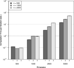
. (c) CD-BLAS, $\lambda=0.3$ (d) PCD-GPU, $\lambda=0.3$

Figure 1: Average computation time per iteration for the AR(2) network. The vertical lines denote 95$\%$ confidence intervals of the mean computation time per iteration.

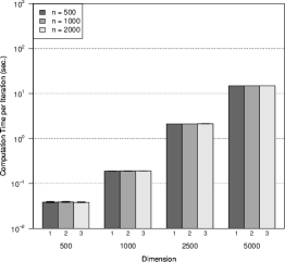
(b) PCD-GPU, $\lambda=0.1$

. (c) CD-BLAS, $\lambda=0.3$ (d) PCD-GPU, $\lambda=0.3$

Figure 2: Average computation time per iteration for the scale-free network. The vertical lines denote 95$\%$ confidence intervals of the mean computation time per iteration.

Note that the efficiency of CD-BLAS depends largely on the efficiency of BLAS (implemented by FORTRAN), as is evident from a comparison between CD-BLAS and CD-NAIVE. For a more precise comparison, we replicate Tables 2 and 3 in Figures 1 and 2, respectively. The figures suggest that CD-BLAS is more sensitive to the sample size compared to PCD-GPU. In the AR(2) network, for example, the computation time per iteration is measured as 0.4886 for $(n,p)=(500,1000)$ and 0.8486 for $(n,p)=(2000,1000)$ with CD-BLAS, but as 0.1817 for $(n,p)=(500,1000)$ and 0.1831 for $(n,p)=(2000,1000)$ with PCD-GPU. This is because the incremental computational burden associated with the sample size is less for each GPU compared to the CPU because a GPU device has many CUDA cores. For example, the GPU device NVIDIA GeForce GTX 1080 Ti used in the numerical studies has 3584 CUDA cores.

In addition, we compared the computation times of the graphical Lasso (GLASSO), which is a popular method in the likelihood approach (Friedman et al.,, 2008), and the constrained $\ell_{1}$-minimization for the inverse of matrix estimation (CLIME), which is the constrained $\ell_{1}$-minimization approach (Cai et al.,, 2011), with ours. For the GLASSO, we used the R package glasso that boosts the original algorithm of Friedman et al., (2008) by adopting block diagonal screening rule (Witten et al.,, 2011). For the CLIME, the original algorithm becomes inefficient when $p$ is large. We apply the FASTCLIME algorithm implemented in R package fastclime Pang et al., (2014), which is more efficient and uses the parametric simplex method to obtain the whole solution path of the CLIME. Since solving the problem of the FASTCLIME is still expensive when $p$ is large, we focus on the cases of $n=500,1000$, $p=500,1000$ and $\lambda=0.3$ for the CONCORD. We choose the tuning parameter $\lambda$s of the GLASSO and the CLIME by searching values that obtain similar sparsity level to that of the CONCORD with $\lambda=0.3$, because the estimators of the GLASSO and CLIME are different to that of the CONCORD. Table 4 reports the averages of the computation times and the number of estimated edges. We found that the proposed PCD-GPU was fastest for AR(2) and the second-best for the scale-free network. For the scale-free network, the efficiency of the proposed PCD-GPU was comparable to that of the GLASSO because the differences in the computation times only lie between 0.24 and 1.01. It has been numerically shown that the CONCORD has better performance than the GLASSO for identifying the non-zero elements of the precision matrix in Khare et al., (2015).

To summarize, we conclude from the our numerical studies that the proposed CONCORD-PCD is adequate for GPU-parallel computation, and more efficient than CONCORD-CD when either the number of variables or the sample size is large. It is also noteworthy that we implemented the PCD algorithm with GPUs by using cuBLAS libary (PCD-GPU-cuBLAS), but we found that the PCD-GPU-cuBLAS was less efficient than the PCD-GPU implemented by our own CUDA kernel functions. Therefore, we have omitted the PCD-GPU-cuBLAS results.

Table 2: Average computation time (in seconds), number of iterations, and number of estimated edges for the AR(2) network. Numbers within parentheses denote standard errors.

$\lambda$	$n$	$p$	Computation time (sec.)				Iteration		$|\hat{E}|$
			CD-BLAS	CD-NAIVE	PCD-CPU	PCD-GPU	CD	PCD	CD	PCD
0.1	500	500	3.22	3.18	3.31	0.89	26.40	26.10	1976.70	1976.70
			(0.02)	(0.02)	(0.02)	(0.01)	(0.16)	(0.18)	(9.52)	(9.52)
		1000	13.09	26.28	28.66	4.87	26.90	26.80	5078.90	5078.90
			(0.09)	(0.17)	(0.18)	(0.04)	(0.18)	(0.20)	(14.19)	(14.19)
		2500	86.01	451.03	513.18	56.72	27.30	27.10	20327.30	20327.50
			(0.83)	(4.30)	(3.28)	(0.38)	(0.26)	(0.18)	(45.87)	(45.90)
		5000	378.04	3646.43	4149.79	404.75	27.70	27.30	64307.20	64307.40
			(2.94)	(19.49)	(51.93)	(2.29)	(0.15)	(0.15)	(69.26)	(69.13)
	1000	500	2.07	3.16	3.29	0.88	25.70	25.50	1407.20	1407.20
			(0.01)	(0.02)	(0.02)	(0.01)	(0.15)	(0.17)	(5.05)	(5.05)
		1000	25.90	25.84	28.27	4.76	26.20	26.10	2825.20	2825.20
			(0.14)	(0.13)	(0.22)	(0.03)	(0.13)	(0.18)	(4.50)	(4.50)
		2500	167.90	428.93	490.24	54.91	26.20	26.20	7216.80	7216.80
			(1.60)	(3.38)	(4.18)	(0.28)	(0.13)	(0.13)	(6.92)	(6.92)
		5000	694.62	3419.50	3862.95	385.66	26.20	26.00	14806.20	14806.20
			(3.87)	(17.43)	(17.96)	(0.05)	(0.13)	(0.00)	(14.28)	(14.28)
	2000	500	2.12	3.19	3.36	0.85	25.00	25.10	1393.10	1393.10
			(0.00)	(0.00)	(0.01)	(0.00)	(0.00)	(0.10)	(3.74)	(3.74)
		1000	21.81	25.76	27.88	4.65	25.70	25.40	2803.10	2803.10
			(0.39)	(0.16)	(0.26)	(0.03)	(0.15)	(0.16)	(4.70)	(4.70)
		2500	342.84	433.35	495.12	54.54	25.90	25.90	7006.90	7006.90
			(1.26)	(1.65)	(1.93)	(0.21)	(0.10)	(0.10)	(9.79)	(9.79)
		5000	1389.95	3440.95	3929.09	386.23	26.00	26.00	14009.30	14009.40
			(6.07)	(13.14)	(11.22)	(0.12)	(0.00)	(0.00)	(9.38)	(9.35)
0.3	500	500	1.69	1.70	1.73	0.50	13.90	13.40	859.50	859.50
			(0.06)	(0.05)	(0.06)	(0.02)	(0.46)	(0.52)	(5.00)	(5.00)
		1000	7.00	14.19	14.80	2.55	14.40	13.70	1722.20	1722.20
			(0.13)	(0.26)	(0.45)	(0.07)	(0.27)	(0.40)	(5.87)	(5.87)
		2500	45.52	240.36	267.74	29.61	14.50	14.10	4297.80	4297.80
			(0.72)	(3.57)	(3.37)	(0.38)	(0.22)	(0.18)	(7.12)	(7.12)
		5000	210.20	1937.84	2289.35	215.59	14.80	14.50	8624.10	8624.10
			(4.05)	(38.32)	(23.56)	(2.47)	(0.29)	(0.17)	(17.08)	(17.08)
	1000	500	1.06	1.59	1.62	0.46	12.40	12.10	853.60	853.60
			(0.02)	(0.03)	(0.03)	(0.01)	(0.22)	(0.23)	(4.66)	(4.66)
		1000	12.06	12.31	13.05	2.22	12.20	11.80	1698.00	1698.00
			(0.13)	(0.13)	(0.15)	(0.02)	(0.13)	(0.13)	(5.80)	(5.80)
		2500	78.69	203.18	225.83	25.51	12.50	12.10	4268.10	4268.10
			(1.56)	(3.53)	(4.36)	(0.48)	(0.22)	(0.23)	(11.70)	(11.70)
		5000	350.79	1718.20	1901.72	182.99	13.00	12.30	8521.50	8521.50
			(7.29)	(35.40)	(39.33)	(3.18)	(0.30)	(0.21)	(11.65)	(11.65)
	2000	500	1.12	1.64	1.62	0.45	11.80	11.00	854.20	854.20
			(0.01)	(0.02)	(0.00)	(0.01)	(0.13)	(0.00)	(3.14)	(3.14)
		1000	10.81	12.22	12.76	2.11	11.60	11.10	1717.00	1717.00
			(0.21)	(0.16)	(0.11)	(0.02)	(0.16)	(0.10)	(4.96)	(4.96)
		2500	159.15	204.24	216.04	24.00	12.00	11.30	4291.10	4291.10
			(0.09)	(0.27)	(1.86)	(0.32)	(0.00)	(0.15)	(5.94)	(5.94)
		5000	637.67	1597.47	1796.61	171.11	12.10	11.50	8578.20	8578.30
			(5.89)	(15.28)	(32.73)	(2.46)	(0.10)	(0.17)	(14.48)	(14.51)

Table 3: Average computation time (in seconds), number of iterations, and number of estimated edges for the scale-free network. Numbers within parentheses denote standard errors.

$\lambda$	$n$	$p$	Computation time (sec.)				Iteration		$|\hat{E}|$
			CD-BLAS	CD-NAIVE	PCD-CPU	PCD-GPU	CD	PCD	CD	PCD
0.1	500	500	1.33	1.35	1.53	0.46	11.30	12.20	2348.30	2348.30
			(0.02)	(0.02)	(0.04)	(0.01)	(0.15)	(0.29)	(13.88)	(13.88)
		1000	5.64	11.41	13.18	2.34	11.90	12.60	8090.90	8090.90
			(0.15)	(0.30)	(0.28)	(0.05)	(0.31)	(0.27)	(22.41)	(22.41)
		2500	43.59	228.30	269.74	30.84	14.20	14.60	42601.50	42601.50
			(1.59)	(8.18)	(9.14)	(1.05)	(0.51)	(0.50)	(34.34)	(34.34)
		5000	193.67	1872.72	2345.42	230.10	14.10	15.50	144508.00	144507.70
			(3.84)	(37.21)	(39.78)	(3.98)	(0.28)	(0.27)	(58.82)	(58.88)
	1000	500	0.96	1.44	1.61	0.48	11.60	12.50	598.20	598.20
			(0.02)	(0.03)	(0.03)	(0.01)	(0.27)	(0.27)	(5.46)	(5.46)
		1000	10.76	11.00	12.49	2.19	11.20	11.70	1340.00	1340.00
			(0.28)	(0.27)	(0.22)	(0.04)	(0.29)	(0.21)	(4.94)	(4.94)
		2500	92.85	235.54	269.49	29.01	13.90	13.70	4471.70	4471.70
			(2.22)	(5.80)	(3.32)	(0.32)	(0.31)	(0.15)	(18.16)	(18.16)
		5000	369.05	1829.25	2121.88	209.48	13.80	14.10	12557.50	12557.60
			(7.76)	(38.16)	(58.87)	(6.02)	(0.29)	(0.41)	(21.90)	(21.94)
	2000	500	1.09	1.60	1.77	0.49	11.90	12.80	506.50	506.50
			(0.01)	(0.02)	(0.02)	(0.01)	(0.18)	(0.20)	(0.50)	(0.50)
		1000	10.62	11.97	12.90	2.18	11.70	11.60	1011.00	1011.00
			(0.25)	(0.20)	(0.32)	(0.05)	(0.21)	(0.31)	(1.02)	(1.02)
		2500	187.80	239.21	257.65	28.62	14.50	13.50	2517.50	2517.50
			(5.47)	(6.88)	(4.20)	(0.47)	(0.43)	(0.22)	(1.56)	(1.56)
		5000	680.01	1705.53	2078.65	209.39	13.10	14.10	5045.90	5045.90
			(9.11)	(23.24)	(26.84)	(2.66)	(0.18)	(0.18)	(2.74)	(2.74)
0.3	500	500	1.03	1.06	1.14	0.37	8.80	9.00	364.70	364.70
			(0.02)	(0.02)	(0.02)	(0.00)	(0.13)	(0.15)	(1.69)	(1.69)
		1000	4.43	9.06	10.14	1.80	9.40	9.60	713.30	713.30
			(0.08)	(0.16)	(0.22)	(0.04)	(0.16)	(0.22)	(2.13)	(2.13)
		2500	34.08	176.28	208.13	22.30	10.50	10.50	1755.40	1755.40
			(0.78)	(3.97)	(3.55)	(0.46)	(0.27)	(0.22)	(5.31)	(5.31)
		5000	138.34	1343.89	1568.08	157.45	10.40	10.60	3569.40	3569.40
			(2.87)	(27.90)	(43.39)	(4.52)	(0.22)	(0.31)	(6.12)	(6.12)
	1000	500	0.77	1.15	1.23	0.37	9.00	9.30	367.80	367.80
			(0.00)	(0.00)	(0.02)	(0.00)	(0.00)	(0.15)	(1.50)	(1.50)
		1000	8.65	8.94	9.75	1.71	9.00	9.00	715.00	715.00
			(0.15)	(0.14)	(0.16)	(0.03)	(0.15)	(0.15)	(2.09)	(2.09)
		2500	68.93	176.52	198.19	21.84	10.50	10.30	1758.80	1758.80
			(1.09)	(2.82)	(3.00)	(0.32)	(0.17)	(0.15)	(2.63)	(2.63)
		5000	267.18	1323.10	1530.87	150.17	9.90	10.10	3582.60	3582.60
			(2.69)	(13.37)	(15.77)	(1.48)	(0.10)	(0.10)	(3.96)	(3.96)
	2000	500	0.87	1.26	1.33	0.38	9.00	9.10	367.30	367.30
			(0.00)	(0.00)	(0.01)	(0.00)	(0.00)	(0.10)	(1.24)	(1.24)
		1000	8.21	9.53	10.43	1.75	9.10	9.20	712.70	712.70
			(0.07)	(0.09)	(0.14)	(0.02)	(0.10)	(0.13)	(1.73)	(1.73)
		2500	134.24	173.16	199.99	22.10	10.40	10.40	1760.00	1760.00
			(2.07)	(2.64)	(3.10)	(0.34)	(0.16)	(0.16)	(3.50)	(3.50)
		5000	513.17	1294.45	1482.85	148.71	9.90	10.00	3585.10	3585.10
			(5.14)	(13.08)	(1.64)	(0.00)	(0.10)	(0.00)	(4.13)	(4.13)

Table 4: Average computation time in seconds (Comp. Time), and number of estimated edges ($|\hat{E}|$) for the AR(2) and scale-free networks for PCD-CPU, PCD-GPU, GLASSO and FASTCLIME. Numbers within parentheses denote standard errors.

Network	$p$	Model	$n=500$			$n=1000$
			$\lambda$	$|\hat{E}|$	Comp. Time	$\lambda$	$|\hat{E}|$	Comp. Time
AR(2)	$500$	PCD-CPU	0.3	859.5	1.73	0.3	1722.2	14.80
				(5.00)	(0.06)		(5.87)	(0.45)
		PCD-GPU	0.3	859.5	0.50	0.3	1722.2	2.55
				(5.00)	(0.02)		(5.87)	(0.07)
		GLASSO	0.383	860.4	0.97	0.386	1711.4	7.57
				(3.50)	(0.00)		(6.36)	(0.02)
		FASTCLIME	0.311	867.3	26.91	0.312	1701.2	198.88
				(3.48)	(0.16)		(7.04)	(0.61)
	$1000$	PCD-CPU	0.3	853.6	1.62	0.3	1698.0	13.05
				(4.66)	(0.03)		(5.80)	(0.15)
		PCD-GPU	0.3	853.6	0.46	0.3	1698.0	2.22
				(4.66)	(0.01)		(5.80)	(0.02)
		GLASSO	0.384	861.5	1.03	0.388	1699.6	7.85
				(3.54)	(0.00)		(5.16)	(0.03)
		FASTCLIME	0.311	854.0	27.25	0.315	1698.4	199.42
				(5.06)	(0.11)		(5.35)	(0.51)
Scale-free	$500$	PCD-CPU	0.3	364.7	1.14	0.3	713.3	10.14
				(1.69)	(0.02)		(2.13)	(0.22)
		PCD-GPU	0.3	364.7	0.37	0.3	713.3	1.80
				(1.69)	(0.00)		(2.13)	(0.04)
		GLASSO	0.241	365.5	0.13	0.249	719.6	0.79
				(2.23)	(0.00)		(1.86)	(0.00)
		FASTCLIME	0.236	364.7	27.29	0.237	717.8	192.89
				(1.56)	(0.07)		(1.81)	(0.18)
	$1000$	PCD-CPU	0.3	367.8	1.23	0.3	715.0	9.75
				(1.50)	(0.02)		(2.09)	(0.16)
		PCD-GPU	0.3	367.8	0.37	0.3	715.0	1.71
				(1.50)	(0.00)		(2.09)	(0.03)
		GLASSO	0.244	368.5	0.19	0.249	707.6	1.01
				(1.67)	(0.00)		(2.50)	(0.00)
		FASTCLIME	0.235	366.6	27.48	0.237	712.6	184.79
				(1.71)	(0.11)		(2.08)	(1.32)

(a) CD-BLAS, $\lambda=0.1$

(b) PCD-GPU, $\lambda=0.1$

(a) CD-BLAS, $\lambda=0.1$

6 Concluding remarks

In this paper, we proposed the parallel coordinate descent algorithm for CONCORD, which simultaneously updates $p_{even}/2$ elements, which is $p/2$ for an even $p$ and $(p-1)/2$ for an odd $p$. We also showed, by applying the theoretical results to edge coloring, that $p_{even}/2$ is the maximum number of simultaneously updatable off-diagonal elements in the CONCORD-CD algorithm. Comprehensive numerical studies show that the proposed CONCORD-PCD algorithm is adequate for GPU-parallel computation, and more efficient than the original CONCORD-CD algorithm, for large datasets.

We conclude the paper with discussion about possible extensions. Our idea of parallelized coordinate descent can be applied to modeling gene regulatory networks from heterogeneous data through joint estimation of sparse precision matrices (Danaher et al.,, 2014). For example, let us consider the following objective function, which estimates two precision matrices, $\Omega_{1}=(\omega_{ij}^{(1)})$ and $\Omega_{2}=(\omega_{ij}^{(2)})$, under the constraint that both matrices are sparse and only slightly different from each other:

$$\begin{array}[]{rcl}\displaystyle L_{joint}(\Omega_{1},\Omega_{2};\lambda_{1},\lambda_{2})&=&\displaystyle\sum_{m=1}^{2}\Big{\{}-\sum_{i=1}^{p}n\log\omega_{ii}^{(m)}+\frac{1}{2}\sum_{i=1}^{p}\sum_{k=1}^{n}\Big{(}\omega_{ii}^{(m)}X_{ki}^{m}+\sum_{j\neq i}\omega_{ij}^{(m)}X_{kj}^{m}\Big{)}^{2}\Big{\}}\\ &&\displaystyle+\lambda_{1}\sum_{m=1}^{2}\sum_{i<j}|\omega_{ij}^{(m)}|+\lambda_{2}\sum_{i\leq j}|\omega_{ij}^{(1)}-\omega_{ij}^{(2)}|,\end{array}$$

where $X_{ki}^{m}$ is the $(k,i)$th element of the observed dataset from $m$th population ($m=1,2$). Consider a block coordinate descent algorithm that minimizes along $(\omega_{ij}^{(1)},\omega_{ij}^{(2)})$ for each update, in which the update formula has a closed-form expression similar to one in Yu et al., (2018). One can show that if two edge indices $ij$ and $i^{\prime}j^{\prime}$ are disjoint, then the update formula for $(\hat{\omega}_{ij}^{(1)},\hat{\omega}_{ij}^{(2)})$ does not involve $(\hat{\omega}_{i^{\prime}j^{\prime}}^{(1)},\hat{\omega}_{i^{\prime}j^{\prime}}^{(2)})$. Thus, one can develop a parallelization for this algorithm as presented in this paper.