Differentially Private Hamiltonian Monte Carlo

Abstract

Markov chain Monte Carlo (MCMC) algorithms have long been the main workhorses of Bayesian inference. Among them, Hamiltonian Monte Carlo (HMC) has recently become very popular due to its efficiency resulting from effective use of the gradients of the target distribution. In privacy-preserving machine learning, differential privacy (DP) has become the gold standard in ensuring that the privacy of data subjects is not violated. Existing DP MCMC algorithms either use random-walk proposals, or do not use the Metropolis–Hastings (MH) acceptance test to ensure convergence without decreasing their step size to zero. We present a DP variant of HMC using the MH acceptance test that builds on a recently proposed DP MCMC algorithm called the penalty algorithm, and adds noise to the gradient evaluations of HMC. We prove that the resulting algorithm converges to the correct distribution, and is ergodic. We compare DP-HMC with the existing penalty, DP-SGLD and DP-SGNHT algorithms, and find that DP-HMC has better or equal performance than the penalty algorithm, and performs more consistently than DP-SGLD or DP-SGNHT.

1 Introduction

Differential privacy (DP) [11] has been widely accepted as the standard approach for developing privacy-preserving algorithms that guarantee that the output of the algorithm cannot be used to violate the privacy of the subjects of the input data. Bayesian inference is one of the widely used approaches for analysis of potentially sensitive data. In this paper, we present the first DP version of the modern Bayesian workhorse, Hamiltonian Monte Carlo (HMC) [7], with provable convergence to the exact posterior under fixed step lengths.

HMC is a Markov chain Monte Carlo (MCMC) algorithm that makes use of gradients of the target density to form a Hamiltonian system that can be accurately simulated numerically to generate very long jumps with a high acceptance rate. HMC scales better to higher dimensions than other MCMC algorithms. New variants [17, 16] that avoid problem-specific tuning make it an ideal choice for efficient and accurate black box inference.

Like all MCMC algorithms, HMC requires careful specification of the algorithm to guarantee convergence to the desired target. This makes the development of DP MCMC algorithms challenging. The first DP MCMC algorithms, such as DP stochastic gradient Langevin dynamics (DP-SGLD) and DP stochastic gradient Nosé-Hoover thermostat (DP-SGNHT), were based on gradient perturbation for stochastic gradient MCMC without a Metropolis–Hastings accept/reject step [28, 19]. These algorithms come with very weak convergence guarantees requiring decreasing the step size to 0.

The first DP MCMC algorithms implementing an accept/reject step that enables convergence with fixed step lengths appeared only in 2019 [29, 15]. Our work builds upon the DP-penalty algorithm [29] that uses the penalty method [3] to compensate for the noise added for DP by decreasing the acceptance rate in a specific way. We adapt the DP-penalty method for HMC, adding DP gradient evaluations. Our main contribution is the proof that the resulting algorithm is ergodic and converges to the desired target.

2 Background

In this section, we introduce main background material relevant to our work. Section 2.1 introduces differential privacy and the privacy accounting method we use. Section 2.2 introduces MH algorithms and the HMC algorithm. Section 2.3 is very technical, and contains the most relevant measure-theoretic background material for our main theorem, the convergence proof of DP-HMC in Theorem 3.3, and a proof that HMC converges to the correct distribution, which serves as a preliminary to Theorem 3.3.

2.1 Differential Privacy

Differential privacy [11] (DP) formalises the notion of a privacy-preserving algorithm by requiring that the distribution of the output only changes slightly given a change to a single individual’s data. Of the many definitions, we use approximate DP (ADP) [10], also known as $(\epsilon,\delta)$-DP:

Definition 2.1.

A mechanism ${\mathcal{M}}\colon{\mathcal{X}}\to\mathbb{R}^{d}$ is $(\epsilon,\delta)$-ADP for neighbourhood relation $\sim$ if for all measurable $S\subset\mathbb{R}^{d}$ and all $X,X^{\prime}\in{\mathcal{X}}$ with $X\sim X^{\prime}$,

$$P({\mathcal{M}}(X)\in S)\leq e^{\epsilon}P({\mathcal{M}}(X^{\prime})\in S)+\delta.$$

We exclusively focus on tabular data and the substitute neighbourhood relation $\sim_{S}$ which means that datasets $X,X^{\prime}\in\mathbb{R}^{n\times d_{x}}$ are neighbors in $\sim_{S}$-relation, $X\sim_{S}X^{\prime}$, if they differ in at most one row. We use $x\in X$ to denote that $x$ is a row of $X$.

DP has two attractive properties: post-processing immunity means that applying a function to the output of a DP mechanism does not change the privacy bounds, and composability means that releasing the output of several DP algorithms together is DP, although with worse privacy bounds [9].

To make HMC DP, we use the Gaussian mechanism [10], together with post-processing immunity and composition.

Definition 2.2.

The Gaussian mechanism with query $f\colon{\mathcal{X}}\to\mathbb{R}^{d}$ and noise variance $\sigma^{2}$ releases a sample from $f(X)+{\mathcal{N}}(0,\sigma^{2}I)$ for input $X$.

To achieve DP, the output of the query of the Gaussian mechanism must not vary too much with changing input: it must have finite sensitivity, and less sensitive queries give smaller privacy bounds.

Definition 2.3.

The $l_{2}$-sensitivity of a function $f\colon{\mathcal{X}}\to\mathbb{R}^{d}$ is defined as

$$\Delta_{2}f=\sup_{X\sim X^{\prime}}||f(X)-f(X^{\prime})||_{2}.$$

To compute the privacy bounds for compositions of several Gaussian mechanisms, we use the tight ADP bound of Sommer et al. [25]:

Theorem 2.4.

Let $f_{i}$ be queries with $\Delta_{2}f_{i}\leq\Delta_{i}$ for $1\leq i\leq k$. Then the composition of $k$ Gaussian mechanisms with queries $f_{i}$ and noise variances $\sigma_{i}^{2}$ for $1\leq i\leq k$ is $(\epsilon,\delta(\epsilon))$-ADP with

$$\delta(\epsilon)=\frac{1}{2}\left(\operatorname{erfc}\left(\frac{\epsilon-\mu}{2\sqrt{\mu}}\right)-e^{\epsilon}\operatorname{erfc}\left(\frac{\epsilon+\mu}{2\sqrt{\mu}}\right)\right),\quad\textrm{where}\quad\mu=\sum_{i=1}^{k}\frac{\Delta_{i}^{2}}{2\sigma_{i}^{2}}.$$

Proof.

The claim follows from three theorems of Sommer et al. [25]: first, the privacy loss distribution (PLD) of a Gaussian mechanism with sensitivity $\Delta$ and noise variance $\sigma^{2}$ is ${\mathcal{N}}(\mu,2\mu)$ with $\mu=\frac{\Delta}{2\sigma^{2}}$. Second, the PLD of a composition of several mechanisms is the convolution of the PLDs of the mechanisms in the composition, so the PLD of a composition of Gaussian mechanisms with PLDs ${\mathcal{N}}(\mu_{i},2\mu_{i})$, $1\leq i\leq k$, is ${\mathcal{N}}(\sum_{i=1}^{k}\mu_{i},2\sum_{i=1}^{k}\mu_{i})$. Finally, a mechanism with a PLD ${\mathcal{N}}(\mu,2\mu)$ is $(\epsilon,\delta(\epsilon))$-ADP with $\delta(\epsilon)$ given by

$$\delta(\epsilon)=\frac{1}{2}\left(\operatorname{erfc}\left(\frac{\epsilon-\mu}{2\sqrt{\mu}}\right)-e^{\epsilon}\operatorname{erfc}\left(\frac{\epsilon+\mu}{2\sqrt{\mu}}\right)\right).\qed$$

In this paper, the query $f\colon\mathbb{R}^{n\times d_{x}}\to\mathbb{R}^{d}$ is always of the summative form $f(X)=\sum_{x\in X}g(x)$ with $g\colon\mathbb{R}^{d_{x}}\to\mathbb{R}^{d}$, so $\Delta_{2}f=\sup_{x,x^{\prime}\in\mathbb{R}^{d_{x}}}||g(x)-g(x^{\prime})||_{2}.$ Moreover, we clip the output of $g$ to have a bounded norm, i.e., instead of the function $g$, we consider the function $\widetilde{g}=\operatorname{clip}_{b}\circ g$, where $\operatorname{clip}_{b}(y)=y\min\{\frac{b}{||y||_{2}},1\}$. Then clearly $\sup_{x,x^{\prime}\in\mathbb{R}^{d_{x}}}||\widetilde{g}(x)-\widetilde{g}(x^{\prime})||_{2}\leq 2b$. Clipping bounds the sensitivity of $f$ and allows adding less noise to the query for equal $(\epsilon,\delta)$-DP guarantees.

2.2 Metropolis-Hastings and Hamiltonian Monte Carlo

Markov chain Monte Carlo (MCMC) algorithms sample from a distribution $\pi$ of $\theta$ by forming an ergodic Markov chain that has the invariant distribution $\pi$ [24]. The Metropolis-Hastings (MH) [20, 14] algorithm constructs the Markov chain by starting from a given point $\theta_{0}$, generating $\theta_{i+1}$ given $\theta_{i}=\theta$ by sampling a proposal $\theta^{\prime}$ from a proposal distribution $q(\theta^{\prime}\mid\theta)$, and accepting the $\theta^{\prime}$ with probability

$$\alpha(\theta,\theta^{\prime})=\min\left\{1,\frac{\pi(\theta^{\prime})}{\pi(\theta)}\frac{q(\theta\mid\theta^{\prime})}{q(\theta^{\prime}\mid\theta)}\right\}.$$

If $\theta^{\prime}$ is accepted, $\theta_{i+1}=\theta^{\prime}$, otherwise $\theta_{i+1}=\theta$.

The invariant distribution of an MH algorithm is always $\pi$, but the ergodicity of the resulting Markov chain depends on the proposal. A convenient sufficient condition for ergodicity is strong irreducibility: if the proposal can propose any state from any other state with positive probability, the chain is said to be strongly ergodic, and thus irreducible [24].

MH is commonly used to sample from the posterior $p(\theta\mid X)$ of a Bayesian inference problem given by Bayes’ theorem:

$$p(\theta\mid X)=\frac{p(X\mid\theta)p(\theta)}{p(X)},$$

where $\theta\in\mathbb{R}^{d}$ denotes the parameters of interest and $X$ denotes the observed data. For the MH algorithm, we set $\pi(\theta)=p(\theta\mid X)$, and the denominator in Bayes’ theorem cancels out in $\alpha(\theta,\theta^{\prime})$, so it is sufficient to consider $\pi(\theta)\propto p(X\mid\theta)p(\theta)$ for the MH algorithm. Usually $X\in\mathbb{R}^{n\times d_{x}}$ with each row of $X$ representing a data point, and the likelihood is $p(X\mid\theta)=\prod_{x\in X}p(x\mid\theta)$, where $x\in X$ means that $x$ is a row of $X$.

The Hamiltonian Monte Carlo (HMC) [7, 22] algorithm is an MH algorithm that generates proposals deterministically through simulating Hamiltonian dynamics. The dynamics are given by the Hamiltonian $H(\theta,p)=U(\theta)+\frac{1}{2}p^{T}M^{-1}p$, where $p\in\mathbb{R}^{d}$ is an auxiliary momentum variable, $M\in\mathbb{R}^{d\times d}$ is a positive-definite mass matrix, and $U(\theta)=-\ln\pi(\theta)$. The simulation is then given by Hamilton’s equations $\frac{\mathrm{d}\theta}{\mathrm{d}t}=M^{-1}p,\frac{\mathrm{d}p}{\mathrm{d}t}=-\nabla U(\theta)$. Solving them exactly is rarely possible, so in practice the simulation is carried out using leapfrog simulation, given for a step-size $\eta>0$ by

$$l=l_{p_{\nicefrac{{\eta}}{{2}}}}\circ l_{\theta}\circ l_{p_{\eta}}\dotsb\circ l_{p_{\eta}}\circ l_{\theta}\circ l_{p_{\nicefrac{{\eta}}{{2}}}},$$

where

$$l_{p_{s}}(\theta,p)=(\theta,p-s\nabla U(\theta)),\quad l_{\theta}(\theta,p)=(\theta+\eta M^{-1}p,p).$$

The definition of $U$ means that $\pi$ is required to be continuous, supported on $\mathbb{R}^{d}$, and have a differentiable log-density [22]. With the auxiliary variable $p$, HMC targets the distribution

$$\pi^{*}(\theta,p)\propto\exp(-H(\theta,p))=\exp(-U(\theta))\exp\left(-\frac{1}{2}p^{T}M^{-1}p\right),$$

so the marginal distributions of $\theta$ and $p$ are independent, the marginal of $\theta$ is $\pi$, and the marginal of $p$ is a $d$-dimensional Gaussian with mean $0$ and covariance $M$.

Proposing a new sample is done in two steps, both of which having a separate MH acceptance test. First, $p$ is sampled from its marginal distribution, which is always accepted. Second, the leapfrog simulation is run and the final value of $p$ is negated, which gives a proposal for $(\theta,p)$. The acceptance probability for the second step is

$$\alpha(\theta,p,\theta^{\prime},p^{\prime})=\min\{1,\exp(H(\theta,p)-H(\theta^{\prime},p^{\prime}))\}.$$

In Section 2.3, we will show that this acceptance probability for the second step makes $\pi^{*}$ the invariant distribution. The proof requires some machinery from measure theory, which is briefly introduced in Section 2.3, and serves as a preliminary to our main result, the DP-HMC convergence proof, in Section 3.

2.3 Convergence of HMC

The proofs of convergence for HMC in Theorem 2.12 and for DP-HMC in Theorem 3.3 require some theory of Markov kernels and their reversibility [5], presented in this section. We defer all proofs to either Appendix A, or the textbook of Çınlar [5], with the exception of the proof of Theorem 2.12, which is fairly short and serves as a preliminary to the proof of our main result in Theorem 3.3.

Recall that a measurable space $(E,{\mathcal{E}})$ is a pair of a set $E$ and a $\sigma$-algebra ${\mathcal{E}}$, and an involution is a function $f$ with $f^{-1}=f$.

Definition 2.5.

Let $(E,{\mathcal{E}})$ be a measurable space and let $q\colon E\times{\mathcal{E}}\to[0,1]$. $q$ is called a Markov kernel on $(E,{\mathcal{E}})$ if

1. For all $B\in{\mathcal{E}}$, the function $q(\cdot,B)$ is measurable.

2. For all $a\in E$, the function $q(a,\cdot)$ is a probability measure.

Markov kernels are the measure-theoreric formulation of random functions. The involutiveness of deterministic functions generalises to reversibility of Markov kernels, as seen in Lemma 2.11.

Definition 2.6.

Let $q$ be a Markov kernel and let $\mu$ be a $\sigma$-finite measure, both on $(E,{\mathcal{E}})$. If

$$\int_{A}\mu(\mathrm{d}a)\int_{B}q(a,\mathrm{d}b)=\int_{B}\mu(\mathrm{d}b)\int_{A}q(b,\mathrm{d}a)$$

for all $A,B\in{\mathcal{E}}$, $q$ is said to be reversible with respect to $\mu$.

Definition 2.6 can be seen as an equality of two measures using a lemma from measure theory:

Lemma 2.7.

Let $(E,{\mathcal{E}})$ be a measurable space and let $q$ be a Markov kernel and $\mu$ be a $\sigma$-finite measure, both on $(E,{\mathcal{E}})$. Then there exists a unique $\sigma$-finite measure $\nu$ on $(E,{\mathcal{E}})^{2}$ such that

$$\nu(A\times B)=\int_{A}\mu(\mathrm{d}a)\int_{B}q(a,\mathrm{d}b)$$

for all $A,B\in{\mathcal{E}}$.

Proof.

See Çınlar [5, Theorem I.6.11]. ∎

Using the uniqueness in Lemma 2.7, the equality in Definition 2.6 can be stated as an equality of measures: for a measurable space $(E,{\mathcal{E}})$, setting

$$\nu_{1}(A\times B)=\int_{A}\mu(\mathrm{d}a)\int_{B}q(a,\mathrm{d}b),$$

$$\nu_{2}(A\times B)=\int_{B}\mu(\mathrm{d}b)\int_{A}q(b,\mathrm{d}a)$$

for all $A,B\in{\mathcal{E}}$ defines unique measures $\nu_{1}$ and $\nu_{2}$ on $(E,{\mathcal{E}})^{2}$. Definition 2.6 is then equivalent to $\nu_{1}=\nu_{2}$.

As Markov kernels represent randomised functions, they can be composed with each other, with the composition being another Markov kernel:

Lemma 2.8.

The composition of Markov kernels $q_{1}$ and $q_{2}$ on a measurable space $(E,{\mathcal{E}})$ is a Markov kernel given by

$$(q_{2}\circ q_{1})(a,C)=\int_{E}q_{1}(a,\mathrm{d}b)q_{2}(b,C)=\int_{E}q_{1}(a,\mathrm{d}b)\int_{C}q_{2}(b,\mathrm{d}c)$$

for any $C\in{\mathcal{E}}$.

Proof.

See Çınlar [5, Remark I.6.4]. ∎

A composition of reversible Markov kernels is not itself reversible, but it does have a closely related property that implies reversibility if the composition is symmetric:

Lemma 2.9.

Let $q_{1},\dotsc,q_{k}$ be Markov kernels on $(E,{\mathcal{E}})$ reversible with respect to a $\sigma$-finite measure $\mu$ on $(E,{\mathcal{E}})$. Then

$$\int_{A}\mu(\mathrm{d}a)\int_{C}(q_{k}\circ\dotsb\circ q_{1})(a,\mathrm{d}c)=\int_{C}\mu(\mathrm{d}c)\int_{A}(q_{1}\circ\dotsb\circ q_{k})(c,\mathrm{d}a)$$

for all $A,C\in{\mathcal{E}}$.

The proposal of an MH algorithm is a Markov kernel. If it is reversible with respect to the Lebesgue measure and the target distribution is continuous, the Hastings correction term $\frac{q(\theta\mid\theta^{\prime})}{q(\theta^{\prime}\mid\theta)}=1$:

Lemma 2.10.

If the proposal Markov kernel $q$ of an MH algorithm is reversible with respect to the Lebesgue measure and the target distribution $\pi$ is continuous, using

$$\alpha(\theta,\theta^{\prime})=\min\left\{1,\frac{\pi(\theta^{\prime})}{\pi(\theta)}\right\}$$

as the acceptance probability leaves the target $\pi$ invariant.

For a deterministic proposal $f$, like the HMC leapfrog, the Markov kernel of the proposal is a Dirac measure $\delta_{f(\theta)}(B)=1_{B}(f(\theta))$ for $\theta\in\mathbb{R}^{d}$ and measurable $B\subset\mathbb{R}^{d}$. It turns out that $\delta_{f(\theta)}$ is a reversible Markov kernel for a suitable $f$:

Lemma 2.11.

Let $f\colon\mathbb{R}^{d}\to\mathbb{R}$ be an involution that preserves Lebesgue measure. Then the Dirac measure $\delta_{f(a)}$, seen as a Markov kernel $q(a,B)=\delta_{f(a)}(B)$, is reversible with respect to the Lebesgue measure.

The invariance of the target distribution for HMC follows from Lemmas 2.10 and 2.11.

Theorem 2.12.

For a continuous distribution $\pi$ that is supported on $\mathbb{R}^{d}$ and has a differentiable log-density, if

$$\alpha(\theta,p,\theta^{\prime},p^{\prime})=\min\{1,\exp(H(\theta,p)-H(\theta^{\prime},p^{\prime}))\}$$

is used as the acceptance probability for HMC, the invariant distribution is $\pi^{*}(\theta,p)\propto\exp(-H(\theta,p))$.

Proof.

The proposal for the second step is given by $l_{-}\circ l$, where $l_{-}(\theta,p)=(\theta,-p)$. As $(l_{-}\circ l)^{-1}=l_{-}\circ l$ [22] and each of $l_{-}$, $l_{p_{s}}$ and $l_{\theta}$ preserve Lebesgue measure, the HMC proposal Markov kernel $\delta_{(l_{-}\circ l)(\theta,p)}$ is reversible with respect to the Lebesgue measure by Lemma 2.11. Then, by Lemma 2.10, $\pi^{*}$ is the invariant distribution of HMC. ∎

Showing that HMC is ergodic is much harder due to the deterministic proposal, but it can be shown that HMC is ergodic with mild assumptions on $U$ [8].

3 DP-HMC

The DP-penalty algorithm of Yildirim and Ermis [29] makes the MH acceptance test private by adding Gaussian noise to the log-likelihood ratio $\lambda(\theta,\theta^{\prime})=\ln\frac{p(X\mid\theta^{\prime})p(\theta^{\prime})}{p(X\mid\theta)p(\theta)}$. They correct the MH acceptance probability with the penalty algorithm [3], that changes the acceptance probability to

$$\alpha(\theta,\theta^{\prime})=\min\left\{1,\exp\left(\lambda(\theta,\theta^{\prime})+\xi+\ln\frac{q(\theta\mid\theta^{\prime})}{q(\theta^{\prime}\mid\theta)}-\frac{1}{2}\sigma_{l}^{2}(\theta,\theta^{\prime})\right)\right\},$$

where $\xi\sim{\mathcal{N}}(0,\sigma_{l}^{2}(\theta,\theta^{\prime}))$ is the Gaussian noise added to the log likelihood ratio. For the DP-penalty algorithm, $\sigma_{l}(\theta,\theta^{\prime})=2\tau b_{l}||\theta-\theta^{\prime}||_{2}$, $b_{l}||\theta-\theta^{\prime}||_{2}$ is the log-likelihood ratio clip bound and $\tau>0$ controls the amount of noise.

The privacy bounds for the algorithm are given by Theorem 2.4 with $\mu_{i}=\frac{1}{2\tau^{2}}$. The convergence of the penalty algorithm requires that the log-likelihood ratios are not actually clipped, which can only be ensured on some models, like Bayesian logistic regression [29]. However, in our experiments shown in Section 4.2, small amounts of clipping did not affect the resulting posterior.

Yildirim and Ermis [29] only used the Gaussian distribution as the proposal, but the DP-penalty algorithm does not require any particular proposal distribution $q$. However, if $q$ depends on the private data $X$, both sampling $q$ and computing $\ln\frac{q(\theta\mid\theta^{\prime})}{q(\theta^{\prime}\mid\theta)}$ may have a privacy cost that must be taken into account.

In non-DP HMC, the proposal is the deterministic leapfrog simulation, which can be made DP by simply clipping the gradients of the log-likelihood and adding Gaussian noise.

In Theorem 3.3, we show that applying the penalty correction to the HMC acceptance probability from Theorem 2.12 results in the correct invariant distribution when using noisy and clipped gradients in the leapfrog simulation. We also prove the ergodicity of DP-HMC, which turns out to be much easier because of the noisy leapfrog, in Theorem 3.4.

In the noisy and clipped leapfrog simulation, the momentum update changes to

$$l_{p_{s}}(\theta,p)=(\theta,p-s(g(\theta)+\xi)),$$

where

$$g(\theta)=\sum_{x\in X}\operatorname{clip}_{b}(\nabla\ln p(x\mid\theta))+\nabla\ln p(\theta)$$

and $\xi\sim{\mathcal{N}}(0,\sigma_{g}^{2})$. The noisy and clipped leapfrog is then

$$l=l_{p_{\nicefrac{{\eta}}{{2}}}}\circ l_{\theta}\circ l_{p_{\eta}}\dotsb\circ l_{p_{\eta}}\circ l_{\theta}\circ l_{p_{\nicefrac{{\eta}}{{2}}}}.$$

As $l_{-}$ is an involution, $l_{-}\circ l$ can be decomposed as

$$l_{-}\circ l=(l_{-}\circ p_{\nicefrac{{\eta}}{{2}}})\circ(l_{\theta}\circ l_{-})\circ(l_{-}\circ l_{p_{\eta}})\dotsb\circ(l_{-}\circ l_{p_{\eta}})\circ(l_{\theta}\circ l_{-})\circ(l_{-}\circ l_{p_{\nicefrac{{\eta}}{{2}}}}).$$

Denoting $l_{p_{s}}^{-}=l_{-}\circ l_{p_{s}}$ and $l_{\theta}^{-}=l_{\theta}\circ l_{-}$, the decomposition can be written as

$$l_{-}\circ l=l_{p_{\nicefrac{{\eta}}{{2}}}}^{-}\circ l_{\theta}^{-}\circ l_{p_{\eta}}^{-}\circ\dotsb\circ l_{p_{\eta}}^{-}\circ l_{\theta}^{-}\circ l_{p_{\nicefrac{{\eta}}{{2}}}}^{-}.$$

This form makes showing that DP-HMC has the correct invariant distribution convenient.

Lemma 3.1.

The Markov kernels $l_{p_{\nicefrac{{\eta}}{{2}}}}^{-}$, $l_{p_{\eta}}^{-}$ and $l_{\theta}^{-}$ are reversible with respect to the Lebesgue measure.

Proof.

The proof is fairly technical, requiring some machinery from measure theory, and is deferred to Appendix A. ∎

Corollary 3.2.

The Markov kernel $l_{-}\circ l$ is reversible with respect to the Lebesgue measure.

Proof.

By Lemma 3.1, the decomposition $l_{-}\circ l=l_{p_{\nicefrac{{\eta}}{{2}}}}^{-}\circ l_{\theta}^{-}\circ l_{p_{\eta}}^{-}\circ\dotsb\circ l_{p_{\eta}}^{-}\circ l_{\theta}^{-}\circ l_{p_{\nicefrac{{\eta}}{{2}}}}^{-}$ fulfills the assumptions of Lemma 2.9. As the decomposition is symmetric, Lemma 2.9 then implies that $l_{-}\circ l$ is reversible with respect to the Lebesgue measure. ∎

Theorem 3.3.

For a continuous distribution $\pi$ that is supported on $\mathbb{R}^{d}$ and has a differentiable log-likelihood, if

$$\alpha_{DP}(\theta,p,\theta^{\prime},p^{\prime})=\min\left\{1,\exp\left(H(\theta,p)-H(\theta^{\prime},p^{\prime})+\xi-\frac{1}{2}\sigma_{l}^{2}(\theta,\theta^{\prime})\right)\right\},$$

where $\xi\sim{\mathcal{N}}(0,\sigma_{l}^{2}(\theta,\theta^{\prime}))$, is used as the acceptance probability of DP-HMC and log-likelihood ratios are not clipped, the invariant distribution is $\pi^{*}(\theta,p)\propto\exp(-H(\theta,p))$.

Proof.

By Corollary 3.2 and Lemma 2.10, using $l_{-}\circ l$ as the proposal of an MH algorithm with

$$\alpha(\theta,p,\theta^{\prime},p^{\prime})=\min\left\{1,\exp\left(H(\theta,p)-H(\theta^{\prime},p^{\prime})\right)\right\}$$

as the acceptance probability makes $\pi^{*}$ the invariant distribution of the algorithm. Applying the DP-penalty algorithm to $\alpha$ results in the acceptance probability

$$\alpha_{DP}(\theta,p,\theta^{\prime},p^{\prime})=\min\left\{1,\exp\left(H(\theta,p)-H(\theta^{\prime},p^{\prime})+\xi-\frac{1}{2}\sigma_{l}^{2}(\theta,\theta^{\prime})\right)\right\},$$

where $\xi\sim{\mathcal{N}}(0,\sigma_{l}^{2}(\theta,\theta^{\prime}))$, leaving $\pi^{*}$ as the invariant distribution. ∎

Like the DP-penalty algorithm, Theorem 3.3 assumes that the log-likelihood ratio is not clipped. This means that convergence is not guaranteed in the presence of clipping, but in practice, we found that clipping a small percentage of the log-likelihood ratios does not affect the resulting posterior, as presented in Section 4.2. Clipping gradients does not affect convergence, but it likely lowers the acceptance rate, thus reducing the utility of any sample.

Theorem 3.4.

DP-HMC is strongly irreducible, and thus ergodic.

Proof.

Consider the last four updates of the leapfrog proposal for $L>1$, $l_{-}\circ l_{p_{\nicefrac{{\eta}}{{2}}}}\circ l_{\theta}\circ l_{p_{\eta}}$. If $L=1$, the first of them will be $l_{p_{\nicefrac{{\eta}}{{2}}}}$ instead, which does not affect the proof. Denote

$$(\theta_{1},p_{1})=l_{p_{\eta}}(\theta_{0},p_{0}),\quad(\theta_{2},p_{2})=l_{\theta}(\theta_{1},p_{1}),\quad(\theta_{3},p_{3})=l_{p_{\nicefrac{{\eta}}{{2}}}}(\theta_{2},p_{2}),\quad(\theta_{4},p_{4})=l_{-}(\theta_{3},p_{3}).$$

Now $\theta_{2}=\theta_{1}+\eta M^{-1}p_{1}$. As $p_{1}\sim{\mathcal{N}}(p_{0}-\eta g(\theta_{0}),\eta^{2}\sigma_{g}^{2})$, and as $M$ is non-singular, $\eta M^{-1}p_{1}$ has a Gaussian distribution with support $\mathbb{R}^{d}$. As $\theta_{1}=\theta_{0}$ and $\theta_{4}=\theta_{3}=\theta_{2}$, it is possible to obtain any value for $\theta_{4}$ no matter the starting point $(\theta_{0},p_{0})$.

Additionally, $p_{4}=-p_{3}\sim{\mathcal{N}}(p_{2}-\frac{\eta}{2}g(\theta_{2}),\frac{\eta^{2}}{4}\sigma_{g}^{2})$, so it is possible to obtain any $p_{4}$ given any $(\theta_{2},p_{2})$. Together, these observations mean that it is possible to obtain any value of $(\theta_{4},p_{4})$ given any starting point $(\theta_{0},p_{0})$. This implies that DP-HMC is strongly irreducible, and thus ergodic [24]. ∎

For non-DP HMC, it is standard practice to perturb $\eta$ between iterations to help the algorithm escape areas where the leapfrog simulation circles back near the starting point that may occur if both $\eta$ and $L$ are kept constant [22]. As $\eta$ will be constant during each leapfrog simulation, this does not affect the invariant distribution of the algorithm. For DP-HMC, we use a randomised Halton sequence [23] to perturb $\eta$ after Hoffman et al. [16], although this may not be as necessary in DP-HMC as the leapfrog simulation is already noisy.

Input: likelihood $p(x\mid\theta)$, prior $p(\theta)$, data $X$, noise parameters $\tau_{l}$ and $\tau_{g}$, clip bounds $b_{l}$ and $b_{g}$, number of iterations $k$, step size sequence $\eta_{i}$ for $1\leq i\leq k$, number of leapfrog steps $L$, positive-definite mass matrix $M$, initial value $\theta_{0}$.

$c_{l}(\theta,\theta^{\prime})=b_{l}||\theta-\theta^{\prime}||_{2}$;

$\sigma_{l}^{2}(\theta,\theta^{\prime})=4\tau_{l}^{2}c_{l}^{2}(\theta,\theta^{\prime})$;

$\sigma_{g}^{2}=4b_{g}^{2}\tau_{g}^{2}$;

for $1\leq i\leq k$ do

       $\theta=\theta_{i-1},\quad$ $\theta^{\prime}=\theta$;

       Sample $p\sim{\mathcal{N}}_{d}(0,M)$ and set $p^{\prime}=p$;

      

      $(\theta^{\prime},p^{\prime})=l_{p_{\nicefrac{{\eta_{i}}}{{2}}}}(\theta^{\prime},p^{\prime})$;

       for $1\leq j\leq L-1$ do

             $(\theta^{\prime},p^{\prime})=l_{\theta}(\theta^{\prime},p^{\prime})$;

             $(\theta^{\prime},p^{\prime})=l_{p_{\eta_{i}}}(\theta^{\prime},p^{\prime})$;

            

      $(\theta^{\prime},p^{\prime})=l_{\theta}(\theta^{\prime},p^{\prime})$;

       $(\theta^{\prime},p^{\prime})=l_{p_{\nicefrac{{\eta_{i}}}{{2}}}}(\theta^{\prime},p^{\prime})$;

      

      $r_{x}=\ln\frac{p(x\mid\theta^{\prime})}{p(x\mid\theta)}$;

       $R=\sum_{x\in X}\operatorname{clip}_{c_{l}(\theta,\theta^{\prime})}(r_{x})$;

       Sample $\xi\sim{\mathcal{N}}(0,\sigma_{l}^{2}(\theta,\theta^{\prime}))$;

       $\Delta p=\frac{1}{2}p^{T}M^{-1}p-\frac{1}{2}p^{\prime T}M^{-1}p^{\prime}$;

       $\Delta H=R+\Delta p+\ln\frac{p(\theta^{\prime})}{p(\theta)}+\xi$;

       Sample $u\sim\mathrm{Unif}(0,1)$;

       if $\ln u<\Delta H-\frac{1}{2}\sigma_{l}^{2}(\theta,\theta^{\prime})$ then

             $\theta_{i}=\theta^{\prime}$;

            

      else

             $\theta_{i}=\theta$;

            

      

return $(\theta_{1},\dotsc,\theta_{k})$;

Algorithm 1 DP-HMC

Algorithm 1 presents DP-HMC. In Algorithm 1, the gradient $\nabla U$ is evaluated $L+1$ times per iteration of the outer for-loop, for a total of $k(L+1)$ times, and the log-likelihood ratio is evaluated $k$ times in total. The privacy cost can then be computed from Theorem 2.4:

Theorem 3.5.

DP-HMC (Algorithm 1) is $(\epsilon,\delta(\epsilon))$-ADP for substitute neighbourhood for

$$\delta(\epsilon)=\frac{1}{2}\left(\operatorname{erfc}\left(\frac{\epsilon-\mu}{2\sqrt{\mu}}\right)-e^{\epsilon}\operatorname{erfc}\left(\frac{\epsilon+\mu}{2\sqrt{\mu}}\right)\right),\quad\textrm{where}\quad\mu=\frac{k}{2\tau_{l}^{2}}+\frac{k(L+1)}{2\tau_{g}^{2}}.$$

Proof.

The sensitivity of the log-likelihood ratio is $2b_{l}||\theta-\theta^{\prime}||_{2}$ and the sensitivity of the gradient is $2b_{g}$. Thus, adding noise with variance $\sigma_{l}^{2}(\theta,\theta^{\prime})$ to the log-likelihood ratio gives a sensitivity-variance ratio $\mu_{l}=\frac{1}{2\tau_{l}^{2}}$. Adding noise with variance $\sigma_{g}^{2}$ to the gradients has sensitivity-variance ratio $\mu_{g}=\frac{1}{2\tau_{l}^{2}}$. As the log-likelihood ratio is evaluated $k$ times and the gradients are evaluated $k(L+1)$ times, the total $\mu$ in Theorem 2.4 is

$$\mu=k\mu_{l}+k(L+1)\mu_{g}=\frac{k}{2\tau_{l}^{2}}+\frac{k(L+1)}{2\tau_{g}^{2}}.\qed$$

It is possible to shave off one gradient evaluation per outer for-loop iteration of Algorithm 1, except the first one, by observing that the first gradient evaluation computed during an outer for-loop iteration is the same gradient as either the first for rejected proposals, or the last for accepted proposals, gradient evaluation of the previous iteration. However, this causes the current iteration to depend on the noise value generated for that gradient evaluation during the previous iteration, so it is not clear whether the resulting chain is Markov. As the potential privacy cost saving from this optimisation is small, we did not investigate this further.

4 Experiments

We ran comparisons on two synthetic posterior distributions, presented in Section 4.1: a 10-dimensional correlated Gaussian model and a banana distribution model that results in a non-convex banana shaped posterior. We also experimented with the effect of clipping log-likelihood ratios, presented in Section 4.2. The code for the experiment is publicly available.

Gaussian Model

The Gaussian is a 10-dimensional model where the prior and likelihood for parameters $\theta\in\mathbb{R}^{d}$ and $X\in\mathbb{R}^{n\times d}$ are given by $\theta\sim{\mathcal{N}}_{d}(\mu_{0},\sigma_{0}^{2}I)$ and $x\sim{\mathcal{N}}_{d}(\theta,\Sigma)$, where $\mu_{0}$ and $\sigma_{0}$ are the prior hyperparameters, and $\Sigma$ is the known variance. As the prior is a Gaussian distribution, the posterior is also a Gaussian with known analytical form [12]. We used $d=10$, $n=100000$, $\mu_{0}=0$, $\sigma_{0}=100$. $\Sigma$ was chosen after Hoffman et al. [16] by sampling its eigenvalues from a gamma distribution with shape parameter $0.5$ and scale parameter 1, and sampling the eigenvectors by orthonormalising the columns of a random matrix with each entry sampled from the uniform distribution on $[0,1]$.

Banana Model

The banana distribution [27] is a probability distribution in the shape of a banana that is a challenging target for MCMC algorithms due to its non-convex and thin shape. The distribution is a transformation of the 2-dimensional Gaussian distribution using the function $g(x_{1},x_{2})=(x_{1},x_{2}-ax_{1}^{2})$. If $x\sim{\mathcal{N}}_{2}(\mu,\Sigma)$, $g(x)$ has the banana distribution denoted by $\operatorname{Ban}(\mu,\Sigma,a)$. To test DP algorithms, we need a Bayesian inference problem where the posterior is a banana distribution. This is given by a transformation of the Gaussian model:

$$\theta=(\theta_{1},\theta_{2})\sim\operatorname{Ban}(0,\sigma_{0}^{2}I,a),\quad x_{1}\sim{\mathcal{N}}(\theta_{1},\sigma_{1}^{2}),\quad x_{2}\sim{\mathcal{N}}(\theta_{2}+a\theta_{1}^{2},\sigma_{2}^{2}).$$

The posterior of this model for data $X\in\mathbb{R}^{n\times 2}$ is $\operatorname{Ban}(\mu,\Sigma,a)$, where, denoting $\tau_{i}=\frac{1}{\sigma_{i}^{2}}$ and $\bar{x}_{i}=\frac{1}{n}\sum_{j=1}^{n}X_{ji}$,

$$\mu=\left(\frac{n\tau_{1}\bar{x}_{1}}{n\tau_{1}+\tau_{0}},\frac{n\tau_{2}\bar{x}_{2}}{n\tau_{2}+\tau_{0}}\right),\quad\Sigma=\operatorname{diag}\left(\frac{1}{n\tau_{1}+\tau_{0}},\frac{1}{n\tau_{2}+\tau_{0}}\right).$$

We used the hyperparameter values $\sigma_{0}=1000$, $\sigma_{1}^{2}=2000$, $\sigma_{2}^{2}=2500$ and $a=20$, $n=100000$ and true parameter values $\theta_{1}=0$, $\theta_{2}=3$.

Evaluation

Our main evaluation metric is maximum mean discrepancy (MMD) [13], which measures the distances between distributions, and can be estimated from a sample of both distributions. We used a Gaussian kernel, and chose the kernel width by choosing a 500 point subsample from both samples with replacement, and used the median between the distances of both subsamples. Additionally, we plot the distance of the mean of the chain and the true posterior sample mean as a more interpretable evaluation metric.

4.1 Comparison of DP-MCMC Algorithms

Detailed implementation

We compare DP-HMC with DP-penalty [29], DP-SGLD [28, 19] and DP-SGNHT [28, 6]. For both models, we ran all algorithms with 4 chains, started from separate starting points. The starting points were chosen by sampling a point from a Gaussian distribution centered on the true parameter values, with standard deviation equal to the mean of the componentwise standard deviations of the reference posterior sample. Each run was repeated 10 times with different with different starting points, but each algorithm and value of $\epsilon$ had the same set of starting points. Algorithm parameters were tuned by manually examining diagnostics from preliminary runs.

Our method of picking starting points close to the area of high probability favors DP-penalty, as the gradient-based methods can use the gradient to quickly find the area of high probability, even when starting far from it. On the other hand, it simulates the effect of finding the rough location of the posterior through another method, such as a MAP estimate or variational inference, with a very small privacy budget, which Heikkilä et al. [15] used in their experiments.

We combined the samples from all 4 chains, discarded the first half as warmup samples, and compared them against 1000 i.i.d. samples from the true posterior. For privacy accounting, we used Theorem 2.4 and Theorem 3.5 for DP-penalty and DP-HMC, respectively. For DP-SGLD and DP-SGNHT, we used the Fourier accountant of Koskela et al. [18] that computes tight privacy bounds for the subsampled Gaussian mechanism. We used $\delta=\frac{0.1}{n}$ for all runs, and varied $\epsilon$. We used a constant step size for DP-SGLD and DP-SGNHT as computing privacy bounds for decreasing step size is infeasible with the Fourier accountant.

Log-likelihood ratio clip bounds for DP-penalty and DP-HMC were tuned to have less than 20% of the log-likelihood ratios clipped, as the clipping experiment in Section 4.2 shows that it leads to minimal effect on the posterior. We used the same guideline for gradient clipping in DP-SGLD and DP-SGNHT, but did not experimentally verify the effect of clipping for them. Gradient clipping for DP-HMC does not affect asymptotic convergence, so it was tuned to minimise the effect of gradient clipping and noise on the acceptance rate.

Results

The top row of Figure 1 shows the result of running each algorithm on the banana model. DP-HMC and DP-penalty have roughly equal performance on both MMD and mean error, while DP-SGLD and DP-SGNHT have significantly worse performance, especially with the higher values of $\epsilon$. The bottom row shows the results with the Gaussian model. The best performer was DP-SGLD, DP-HMC and DP-SGNHT were mostly equal, and DP-penalty performed the worst.

Figure 2 compares the posteriors from each algorithm with $\epsilon=15$ to the true posterior on the banana model. The comparison shows the reason for the poor performance of DP-SGLD and DP-SGNHT: they have trouble exploring the long tail of the posterior. The median sample of DP-penalty highlights one of the difficulties in sampling the banana model: the sample seems to cover the posterior well from the 2D plot, but the marginal plots reveal that it overrepresents the tail, which is likely a result of one of the chains getting stuck in the tail. DP-HMC is more consistent in this regard.

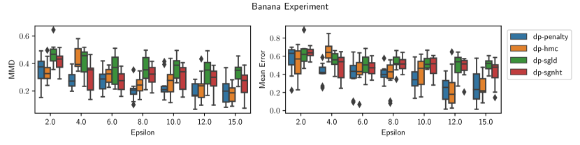
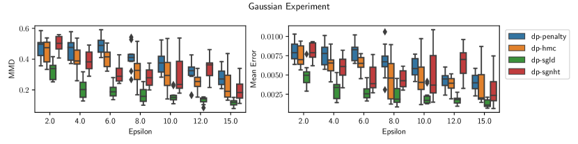
Figure 1: MMD and mean error for the banana and Gaussian models.

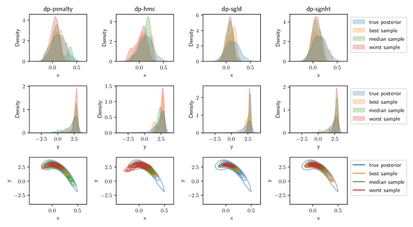
Figure 2: Visual comparison of the posteriors from each algorithm and the true posterior with $\epsilon=15$. The top and middle rows show KDE plots of the marginal distributions for the best, median and worst samples by MMD compared to the reference posterior sample. The bottom row shows a 2D KDE of each sample compared to the reference posterior sample.

4.2 Clipping Experiment

Implementation

To asses the effect of clipping log-likelihood ratios, we ran random walk Metropolis-Hastings (RWMH) and HMC on both the banana and Gaussian models while clipping log-likelihood ratios. We did not add noise at any point, and used a large gradient clip bound for HMC, to isolate the effect of log-likelihood ratio clipping. We chose the number of iterations and parameters for the algorithms by ensuring that they converge in the sense that $\hat{R}<1.05$ [12], and ran the algorithms with varying clip bounds. Otherwise, we used the same setup as with the main experiments in Section 4: we ran 4 chains for each triple of clip bound, algorithm and model, and computed the MMD of the combined sample from all chains, with the first half of each chain discarded. Each run was repeated 10 times, with the same starting points as the main experiment.

Results

Figure 3 shows the results of the clipping experiment. With a large enough clip bound, there is very little effect on the MMD, as seen on the left side panels. The right side panels show MMD as a function of the fraction of log-likelihood ratios that were clipped, which shows that clipping has very little effect when less than 20% of the log-likelihood ratios are clipped, which we used as our guideline for tuning the clip bounds for our main experiments. Not all of runs converged, especially with the smaller clip bounds, as we only set the parameters for the largest clip bound.

Based on the 20% guideline, for the experiments of Section 4, we set the clip bounds 0.1 and 6 for DP-HMC on the banana and Gaussian, respectively, and 0.15 and 10 for DP-penalty on the banana and Gaussian, respectively. Based on Figure 3, there should be minimal effect from clipping at those bounds.

There is an interesting contrast in the results for the banana and Gaussian models in Figure 3. On the Gaussian model, there is a gap in the fractions of clipped log-likelihood ratios between 0.2 and 0.6, while it is not present with the banana. This could be a result of fact that the Gaussian experiment does not have any clip bounds between 1 and 5, which is a fairly large jump.

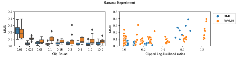
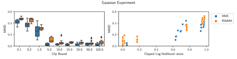
Figure 3: Results for the clipping experiment. The left side shows MMD as a function of clip bound, while the right side shows MMD as a function of the fraction of log-likelihood ratios that were clipped. Each point represents one of the 10 runs for each triple of clip bound, algorithm and model.

5 Discussion

Limitations

Our experiment in Section 4 show that the MH acceptance test is useful for efficient exploration of the tails of the banana posterior. However, we had to use very large values of $\epsilon$ to make any progress towards sampling from the entire posterior, so it is clear that DP-MCMC methods cannot achieve comparable performance to non-DP methods, unless very loose privacy bounds are used, or a very large dataset $(n\gg 10^{5})$ is used. We also noticed that the acceptance rates for DP-penalty and DP-HMC drop rapidly with increasing dimension on the Gaussian model, which is why we used a fairly low number of dimensions ($d=10$). This is a major limitation that warrants further investigation.

Another major limitation of our work is our reliance on the Gaussian mechanism, which is likely vulnerable to floating point inaccuracies in computer implementations that destroy the theoretical privacy guarantees [21]. The discrete Gaussian mechanism [2] can be used in place of the Gaussian mechanism for many applications, but the penalty algorithm requires adding Gaussian noise, so the discrete Gaussian cannot be used as a drop-in replacement.

Future research

There are many potential improvements to DP-HMC. Subsampling the gradients, as is done in DP-SGLD and DP-SGNHT, would provide a significant privacy budget saving. However, naive gradient subsampling is likely to lower acceptance rates significantly, especially in high dimensions [1]. The SGHMC [4] and SGNHT [6] algorithms correct for gradient subsampling by adding friction to the Hamiltonian dynamics, but they forego the MH acceptance test. Conducting the MH test with the added friction is not trivial, but it has been done for SGHMC in the AMAGOLD algorithm [30].

Heikkilä et al. [15] used subsampling in the acceptance test of their DP MCMC algorithm by assuming that the error from subsampling is close to Gaussian by the central limit theorem. The same justification could be applied to the penalty algorithm, but in our preliminary experiments it substantially lowered the acceptance rate and did not improve the overall results.

Other potential improvements for DP-HMC are tuning the parameters, especially $\eta$ and $L$, automatically. NUTS [17] is the most famous HMC variant that tunes $\eta$ and $L$ automatically, but it has a very complicated sampling process. The recent ChEES-HMC algorithm [16] has a much simpler automatic tuning process, making it more suitable for integration into DP-HMC.

6 Conclusion

We developed DP-HMC, a DP variant of HMC, and proved that it has the correct invariant distribution and is ergodic in Section 3. In Section 4, we compared DP-HMC with existing DP-MCMC algorithms, and showed that DP-HMC is consistently better or equal to DP-penalty, while DP-SGLD and DP-SGNHT did not perform consistently.

Appendix A Measure Theory

In this section, we prove the measure-theoretic results stated in the main text but not proved there. We start by recalling the main definitions of Section 2.3: See 2.5 See 2.6

Lemma A.1.

Let $q_{1}$ and $q_{2}$ be Markov kernels on $(E,{\mathcal{E}})$, let $\mu$ be a $\sigma$-finite measure, and let $f\colon E\times E\to\mathbb{R}_{+}$ be a measurable function. If

$$\int_{A}\mu(\mathrm{d}a)\int_{B}q_{1}(a,\mathrm{d}b)=\int_{B}\mu(\mathrm{d}b)\int_{A}q_{2}(b,\mathrm{d}a),$$

for all $A,B\in{\mathcal{E}}$, then

$$\int_{A}\mu(\mathrm{d}a)\int_{B}q_{1}(a,\mathrm{d}b)f(a,b)=\int_{B}\mu(\mathrm{d}b)\int_{A}q_{2}(b,\mathrm{d}a)f(a,b)$$

for all $A,B\in{\mathcal{E}}$.

Proof.

The condition

$$\int_{A}\mu(\mathrm{d}a)\int_{B}q_{1}(a,\mathrm{d}b)=\int_{B}\mu(\mathrm{d}b)\int_{A}q_{2}(b,\mathrm{d}a)$$

means that the measures (as in Lemma 2.7)

$$\nu_{1}(A\times B)=\int_{A}\mu(\mathrm{d}a)\int_{B}q(a,\mathrm{d}b),$$

$$\nu_{2}(A\times B)=\int_{B}\mu(\mathrm{d}b)\int_{A}q(b,\mathrm{d}a)$$

are equal. Then

$$\int_{A}\mu(\mathrm{d}a)\int_{B}q_{1}(a,\mathrm{d}b)f(a,b) =\int_{A\times B}\nu_{1}(\mathrm{d}a,\mathrm{d}b)f(a,b)$$

$$=\int_{A\times B}\nu_{2}(\mathrm{d}a,\mathrm{d}b)f(a,b)$$

$$=\int_{B}\mu(\mathrm{d}b)\int_{A}q_{2}(b,\mathrm{d}a)f(a,b)$$

for all $A,B\in{\mathcal{E}}$. ∎

Corollary A.2.

Let $q$ be a Markov kernel on $(E,{\mathcal{E}})$ reversible with respect to a $\sigma$-finite measure $\mu$. Then

$$\int_{A}\mu(\mathrm{d}a)\int_{B}q(a,\mathrm{d}b)f(a,b)=\int_{B}\mu(\mathrm{d}b)\int_{A}q(b,\mathrm{d}a)f(a,b)$$

for all $A,B\in{\mathcal{E}}$.

Proof.

The claim follows by setting $q_{1}=q_{2}=q$ in Lemma A.1, as the condition of Lemma A.1 is then the reversibility of $q$ with respect to $\mu$. ∎

See 2.9

Proof.

We prove the claim by induction on $k$. For $k=1$, the claim is the definition of reversibility of $q_{1}$ with respect to $\mu$. If the claim holds for $k-1$, for any $A,C\in{\mathcal{E}}$,

$$\int_{A}\mu(\mathrm{d}a)\int_{C}(q_{k}\circ\dotsb\circ q_{1})(a,\mathrm{d}c) =\int_{A}\mu(\mathrm{d}a)\int_{E}(q_{k-1}\circ\dotsb\circ q_{1})(a,\mathrm{d}b)\int_{C}q_{k}(b,\mathrm{d}c)$$ (1)

$$=\int_{E}\mu(\mathrm{d}b)\int_{A}(q_{1}\circ\dotsb\circ q_{k-1})(b,\mathrm{d}a)\int_{C}q_{k}(b,\mathrm{d}c)$$ (2)

$$=\int_{E}\mu(\mathrm{d}b)\int_{C}q_{k}(b,\mathrm{d}c)\int_{A}(q_{1}\circ\dotsb\circ q_{k-1})(b,\mathrm{d}a)$$ (3)

$$=\int_{C}\mu(\mathrm{d}c)\int_{E}q_{k}(c,\mathrm{d}b)\int_{A}(q_{1}\circ\dotsb\circ q_{k-1})(b,\mathrm{d}a)$$ (4)

$$=\int_{C}\mu(\mathrm{d}c)\int_{A}(q_{1}\circ\dotsb\circ q_{k})(c,\mathrm{d}a).$$ (5)

Lines (1) and (5) follow from Lemma 2.8, line (2) from the induction hypothesis and Lemma A.1, and line (4) from Corollary A.2. ∎

See 2.10

Proof.

For acceptance probability $\alpha$, the detailed balance condition

$$\int_{A}\pi(\mathrm{d}\theta)\int_{B}q(\theta,\mathrm{d}\theta^{\prime})\alpha(\theta,\theta^{\prime})=\int_{B}\pi(\mathrm{d}\theta^{\prime})\int_{A}q(\theta^{\prime},\mathrm{d}\theta)\alpha(\theta^{\prime},\theta)$$

for all measurable $A,B\subset\mathbb{R}^{d}$ implies the invariance of $\pi$ [26]. If $\pi$ is continuous and $q$ is reversible with respect to the Lebesgue measure $m$, for measurable $A,B\subset\mathbb{R}^{d}$:

$$\int_{A}\pi(\mathrm{d}\theta)\int_{B}q(\theta,\mathrm{d}\theta^{\prime})\alpha(\theta,\theta^{\prime}) =\int_{A}m(\mathrm{d}\theta)\int_{B}\pi(\theta)q(\theta,\mathrm{d}\theta^{\prime})\alpha(\theta,\theta^{\prime})$$

$$=\int_{A}m(\mathrm{d}\theta)\int_{B}q(\theta,\mathrm{d}\theta^{\prime})\min\{\pi(\theta),\pi(\theta^{\prime})\}$$

$$=\int_{B}m(\mathrm{d}\theta^{\prime})\int_{A}q(\theta^{\prime},\mathrm{d}\theta)\min\{\pi(\theta^{\prime}),\pi(\theta)\}$$

$$=\int_{B}\pi(\mathrm{d}\theta^{\prime})\int_{A}q(\theta^{\prime},\mathrm{d}\theta)\alpha(\theta^{\prime},\theta),$$

which implies the invariance of $\pi$. ∎

See 2.11

Proof.

As $f=f^{-1}$ and preserves Lebesgue measure, for all measurable $A,B\subset\mathbb{R}^{d}$:

$$\int_{A}m(\mathrm{d}a)\int_{B}\delta_{f(a)}(\mathrm{d}b) =\int_{A}m(\mathrm{d}a)1_{B}(f(a))$$

$$=m(A\cap f^{-1}(B))$$

$$=m(f^{-1}(A\cap f^{-1}(B)))$$

$$=m(f^{-1}(A)\cap B)$$

$$=\int_{B}m(\mathrm{d}b)\int_{A}\delta_{f(b)}(\mathrm{d}a).\qed$$

For the convergence proof of DP-HMC, specifically Lemma 3.1, we must deal with Markov kernels defined on $\mathbb{R}^{2d}$ that have the auxiliary variable $p$ in addition to the parameter $\theta$. The preceding theory cannot deal with both variables separately, so we must develop theory that can, which culminates in Lemma A.6.

Definition A.3.

Let $E$ be a set. A collection $\mathcal{C}\subset\mathcal{P}(E)$ is called a p-system if $A\cap B\in\mathcal{C}$ for all $A,B\in\mathcal{C}$.

Lemma A.4.

Let $E$ be a set and let $\mathcal{C}\subset\mathcal{P}(E)$ be a p-system. Let ${\mathcal{E}}$ be the $\sigma$-algebra generated by $\mathcal{C}$. Let $\mu$ and $\nu$ be finite measures on $(E,{\mathcal{E}})$. If $\mu(A)=\nu(A)$ for all $A\in\mathcal{C}$, $\mu=\nu$.

Proof.

See Çınlar [5, Proposition I.3.7]. ∎

Lemma A.5.

Let $(E,{\mathcal{E}})$ be a measurable space and let $\mu$ and $\nu$ be measures on $(E,{\mathcal{E}})^{d}$ with a countable partition $P$ of $E$ such that $\mu(\operatorname*{\times}_{j=1}^{d}B_{j})<\infty$ and $\nu(\operatorname*{\times}_{j=1}^{d}B_{j})<\infty$ for all $B_{1},\dotsc,B_{d}\in P$. If

$$\mu\left(\operatorname*{\times}_{j}^{d}A_{j}\right)=\nu\left(\operatorname*{\times}_{j}^{d}A_{j}\right)$$

for all $A_{1},\dotsc,A_{d}\in{\mathcal{E}}$, $\mu=\nu$.

Proof.

Let $P_{d}=\{\operatorname*{\times}_{j=1}^{d}B_{j}\mid B_{1},\dotsc,B_{d}\in P\}$. Denote the restriction of $\mu$ into $C$ by $\mu|C$, which is the measure $(\mu|C)(A)=\mu(A\cap C)$ [5]. The measures $\mu|C$ and $\nu|C$ for $C\in P_{d}$ are finite as $(\mu|C)(A)\leq\mu(C)<\infty$ for any $A\in{\mathcal{E}}^{d}$ and the same holds for $\nu$.

Recall that ${\mathcal{E}}^{d}$ is generated by the p-system of sets of the form $\operatorname*{\times}_{j=1}^{d}A_{j}$ for $A_{1},\dotsc,A_{d}\in{\mathcal{E}}$. For any $C\in P_{d}$ and $A_{1},\dotsc,A_{d}\in{\mathcal{E}}$, we have

$$(\mu|C)\left(\operatorname*{\times}_{j=1}^{d}A_{j}\right) =\mu\left(\left(\operatorname*{\times}_{j=1}^{d}A_{j}\right)\cap\left(\operatorname*{\times}_{j=1}^{d}B_{j}\right)\right)$$

$$=\mu\left(\operatorname*{\times}_{j=1}^{d}(A_{j}\cap B_{j})\right)$$

$$=\nu\left(\operatorname*{\times}_{j=1}^{d}(A_{j}\cap B_{j})\right)$$

$$=(\nu|B)\left(\operatorname*{\times}_{j=1}^{d}A_{j}\right),$$

so $(\mu|C)=(\nu|C)$ for any $C\in P_{d}$ by Lemma A.4.

As $P$ is countable, the sets in $P_{d}$ can be enumerated as $C_{i}$ for $i\in\mathbb{N}$. Now

$$\mu(A)=\mu(E^{d}\cap A)=\mu\left(\bigcup_{i=1}^{\infty}(C_{i}\cap A)\right)=\sum_{i=1}^{\infty}(\mu|C_{i})(A)=\sum_{i=1}^{\infty}(\nu|C_{i})(A)=\nu(A)$$

for any $A\in{\mathcal{E}}^{d}$, so $\mu=\nu$. ∎

Lemma A.6.

Let $(E,{\mathcal{E}})$ be a measurable space, let $q$ be a Markov kernel on $(E,{\mathcal{E}})^{2}$ and let $\mu$ be a $\sigma$-finite measure on $(E,{\mathcal{E}})$. Then $q$ is reversible with respect to $\mu^{2}$ if and only if

$$\int_{A}\mu(\mathrm{d}a)\int_{B}\mu(\mathrm{d}b)\int_{C\times D}q((a,b),\mathrm{d}(c,d))=\int_{C}\mu(\mathrm{d}c)\int_{D}\mu(\mathrm{d}d)\int_{A\times B}q((c,d),\mathrm{d}(a,b))$$

for all $A,B,C,D\in E$.

Proof.

Let $V,W\in{\mathcal{E}}^{2}$ and

$$\nu_{1}(V\times W)=\int_{V}\mu^{2}(\mathrm{d}v)\int_{W}q(v,\mathrm{d}w),$$

$$\nu_{2}(V\times W)=\int_{W}\mu^{2}(\mathrm{d}w)\int_{V}q(w,\mathrm{d}v).$$

Now reversibility of $q$ with respect to $\mu^{2}$ is equivalent to $\nu_{1}=\nu_{2}$.

If $\nu_{1}=\nu_{2}$, for all $A,B,C,D\in{\mathcal{E}}$,

$$\int_{A}\mu(\mathrm{d}a)\int_{B}\mu(\mathrm{d}b)\int_{C\times D}q((a,b),\mathrm{d}(c,d)) =\nu_{1}(A\times B\times C\times D)$$

$$=\nu_{2}(A\times B\times C\times D)$$

$$=\int_{C}\mu(\mathrm{d}c)\int_{D}\mu(\mathrm{d}d)\int_{A\times B}q((c,d),\mathrm{d}(a,b)).$$

If

$$\int_{A}\mu(\mathrm{d}a)\int_{B}\mu(\mathrm{d}b)\int_{C\times D}q((a,b),\mathrm{d}(c,d))=\int_{C}\mu(\mathrm{d}c)\int_{D}\mu(\mathrm{d}d)\int_{A\times B}q((c,d),\mathrm{d}(a,b)),$$

then

$$\nu_{1}(A\times B\times C\times D)=\nu_{2}(A\times B\times C\times D)$$

for all $A,B,C,D\in{\mathcal{E}}$. As $\mu$ is $\sigma$-finite, there is a countable partition $E_{i}$ of $E$ such that $\mu(E_{i})<\infty$ for all $i\in\mathbb{N}$. Additionally,

$$\nu_{1}(E_{i}\times E_{j}\times E_{k}\times E_{l})\leq\int_{E_{i}}\mu(\mathrm{d}a)\int_{E_{j}}\mu(\mathrm{d}b)<\infty$$

and

$$\nu_{2}(E_{i}\times E_{j}\times E_{k}\times E_{l})\leq\int_{E_{k}}\mu(\mathrm{d}c)\int_{E_{l}}\mu(\mathrm{d}d)<\infty.$$

so $\nu_{1}=\nu_{2}$ by Lemma A.5. ∎

See 3.1

Proof.

Starting with $l_{\theta}^{-}=l_{\theta}\circ l_{-}$, note that $l_{\theta}\circ l_{-}$ is an involution that preserves Lebesgue measure. The Markov kernel for $l_{\theta}\circ l_{-}$ is $\delta_{(l_{\theta}\circ l_{-}})(\theta,p)$, so the claim follows from Lemma 2.11.

Recall that both $l_{p_{\nicefrac{{\eta}}{{2}}}}^{-}$ and $l_{p_{\eta}}^{-}$ are of the form

$$(l_{-}\circ l_{p_{s}})(\theta,p)=(\theta,-p+s(g(\theta)+\xi)),$$

where $\xi\sim{\mathcal{N}}(0,\sigma_{g}^{2})$ and $s>0$. Definition 2.6 for $l_{-}\circ l_{p_{s}}$ is

$$\int_{V}m_{2d}(\mathrm{d}v)\int_{W}(l_{-}\circ l_{p_{s}})(v,\mathrm{d}w)=\int_{W}m_{2d}(\mathrm{d}w)\int_{V}(l_{-}\circ l_{p_{s}})(w,\mathrm{d}v)$$

for all measurable $V,W\in\mathbb{R}^{2d}$. Because of Lemma A.6, this can be stated as

$$\int_{A}m_{d}(\mathrm{d}\theta)\int_{B}m(\mathrm{d}p)\int_{C\times D}(l_{-}\circ l_{p_{s}})(\theta,p,\mathrm{d}(\theta^{\prime},p^{\prime}))$$

$$= \int_{C}m_{d}(\mathrm{d}\theta^{\prime})\int_{D}m(\mathrm{d}p^{\prime})\int_{A\times B}(l_{-}\circ l_{p_{s}})(\theta^{\prime},p^{\prime},\mathrm{d}(\theta,p))$$

for all measurable $A,B,C,D\subset\mathbb{R}^{d}$. Denote $f(\theta)=sg(\theta)$, $\sigma^{2}=s^{2}\sigma_{g}^{2}$ and the density function of the $d$-dimensional Gaussian distribution by ${\mathcal{N}}(\cdot\mid\mu,\Sigma)$. Now, for any measurable $C,D\subset\mathbb{R}^{d}$

$$\int_{C\times D}(l_{-}\circ l_{p_{s}})(\theta,p,\mathrm{d}(\theta^{\prime},p^{\prime})) =1_{C}(\theta)\int_{D}m_{d}(\mathrm{d}p^{\prime}){\mathcal{N}}_{d}(p^{\prime}\mid-p+f(\theta),\sigma^{2}I)$$ (6)

$$=\int_{C}\delta_{\theta}(\mathrm{d}\theta^{\prime})\int_{D}m_{d}(\mathrm{d}p^{\prime}){\mathcal{N}}_{d}(p^{\prime}\mid-p+f(\theta),\sigma^{2}I),$$ (7)

which leads into

$$\int_{A}m_{d}(\mathrm{d}\theta)\int_{B}m_{d}(\mathrm{d}p)\int_{C\times D}(l_{-}\circ l_{p_{s}})(\theta,p,\mathrm{d}(\theta^{\prime},p^{\prime}))$$ (8)

$$=\int_{A}m_{d}(\mathrm{d}\theta)\int_{B}m_{d}(\mathrm{d}p)\int_{C}\delta_{\theta}(\mathrm{d}\theta^{\prime})\int_{D}m_{d}(\mathrm{d}p^{\prime}){\mathcal{N}}_{d}(p^{\prime}\mid-p+f(\theta),\sigma^{2}I)$$ (9)

$$=\int_{A}m_{d}(\mathrm{d}\theta)\int_{C}\delta_{\theta}(\mathrm{d}\theta^{\prime})\int_{B}m_{d}(\mathrm{d}p)\int_{D}m_{d}(\mathrm{d}p^{\prime}){\mathcal{N}}_{d}(p^{\prime}\mid-p+f(\theta),\sigma^{2}I)$$ (10)

$$=\int_{C}m_{d}(\mathrm{d}\theta^{\prime})\int_{A}\delta_{\theta^{\prime}}(\mathrm{d}\theta)\int_{B}m_{d}(\mathrm{d}p)\int_{D}m_{d}(\mathrm{d}p^{\prime}){\mathcal{N}}_{d}(p^{\prime}\mid-p+f(\theta),\sigma^{2}I)$$ (11)

$$=\int_{C}m_{d}(\mathrm{d}\theta^{\prime})\int_{A}\delta_{\theta^{\prime}}(\mathrm{d}\theta)\int_{B}m_{d}(\mathrm{d}p)\int_{D}m_{d}(\mathrm{d}p^{\prime}){\mathcal{N}}_{d}(p\mid-p^{\prime}+f(\theta),\sigma^{2}I)$$ (12)

$$=\int_{C}m_{d}(\mathrm{d}\theta^{\prime})1_{A}(\theta^{\prime})\int_{B}m_{d}(\mathrm{d}p)\int_{D}m_{d}(\mathrm{d}p^{\prime}){\mathcal{N}}_{d}(p\mid-p^{\prime}+f(\theta^{\prime}),\sigma^{2}I)$$ (13)

$$=\int_{C}m_{d}(\mathrm{d}\theta^{\prime})\int_{D}m_{d}(\mathrm{d}p^{\prime})1_{A}(\theta^{\prime})\int_{B}m_{d}(\mathrm{d}p){\mathcal{N}}_{d}(p\mid-p^{\prime}+f(\theta^{\prime}),\sigma^{2}I)$$ (14)

$$=\int_{C}m_{d}(\mathrm{d}\theta^{\prime})\int_{D}m(\mathrm{d}p^{\prime})\int_{A\times B}(l_{-}\circ l_{p_{s}})(\theta^{\prime},p^{\prime},\mathrm{d}(\theta,p)),$$ (15)

where (11) uses Lemma A.2, (13) uses the property of the Dirac measure that $\int_{A}\delta_{b}(\mathrm{d}a)f(a)=1_{A}(b)f(b)$ for $f\colon\mathbb{R}^{d}\to\mathbb{R}^{d}$ and (15) uses Equation (6). ∎

References

• Betancourt [2015] Michael Betancourt. The fundamental incompatibility of scalable Hamiltonian Monte Carlo and naive data subsampling. In Proceedings of the 32nd International Conference on Machine Learning, volume 37 of JMLR Workshop and Conference Proceedings, pages 533–540. 2015.
• Canonne et al. [2020] Clément L. Canonne, Gautam Kamath, and Thomas Steinke. The discrete Gaussian for differential privacy. In Advances in Neural Information Processing Systems 33: Annual Conference on Neural Information Processing Systems, 2020.
• Ceperley and Dewing [1999] DM Ceperley and Mark Dewing. The penalty method for random walks with uncertain energies. The Journal of chemical physics, 110(20):9812–9820, 1999.
• Chen et al. [2014] Tianqi Chen, Emily B. Fox, and Carlos Guestrin. Stochastic gradient Hamiltonian Monte Carlo. In Proceedings of the 31th International Conference on Machine Learning, volume 32 of JMLR Workshop and Conference Proceedings, pages 1683–1691. 2014.
• Çınlar [2011] Erhan Çınlar. Probability and Stochastics. Graduate Texts in Mathematics, 261. Springer New York, New York, NY, 1st edition, 2011.
• Ding et al. [2014] Nan Ding, Youhan Fang, Ryan Babbush, Changyou Chen, Robert D. Skeel, and Hartmut Neven. Bayesian sampling using stochastic gradient thermostats. In Advances in Neural Information Processing Systems 27: Annual Conference on Neural Information Processing Systems, pages 3203–3211, 2014.
• Duane et al. [1987] Simon Duane, Anthony D Kennedy, Brian J Pendleton, and Duncan Roweth. Hybrid Monte Carlo. Physics letters B, 195(2):216–222, 1987.
• Durmus et al. [2020] Alain Durmus, Eric Moulines, and Eero Saksman. Irreducibility and geometric ergodicity of Hamiltonian Monte Carlo. Annals of Statistics, 48(6):3545–3564, 2020.
• Dwork and Roth [2014] Cynthia Dwork and Aaron Roth. The algorithmic foundations of differential privacy. Foundations and Trends in Theoretical Computer Science, 9(3-4):211–407, 2014.
• Dwork et al. [2006a] Cynthia Dwork, Krishnaram Kenthapadi, Frank McSherry, Ilya Mironov, and Moni Naor. Our data, ourselves: Privacy via distributed noise generation. In Advances in Cryptology - EUROCRYPT 2006, 25th Annual International Conference on the Theory and Applications of Cryptographic Techniques, volume 4004 of Lecture Notes in Computer Science, pages 486–503. 2006a.
• Dwork et al. [2006b] Cynthia Dwork, Frank McSherry, Kobbi Nissim, and Adam D. Smith. Calibrating noise to sensitivity in private data analysis. In Theory of Cryptography, Third Theory of Cryptography Conference, TCC, volume 3876 of Lecture Notes in Computer Science, pages 265–284. 2006b.
• Gelman et al. [2014] Andrew Gelman, John B Carlin, Hal S Stern, David B Dunson, Aki Vehtari, and Donald B Rubin. Bayesian data analysis. Chapman & Hall/CRC texts in statistical science series. CRC Press, Boca Raton, third edition, 2014.
• Gretton et al. [2012] Arthur Gretton, Karsten M. Borgwardt, Malte J. Rasch, Bernhard Schölkopf, and Alexander J. Smola. A kernel two-sample test. J. Mach. Learn. Res., 13:723–773, 2012.
• Hastings [1970] W.K. Hastings. Monte Carlo sampling methods using Markov chains and their applications. Biometrika, 57(1):97–109, 1970.
• Heikkilä et al. [2019] Mikko A. Heikkilä, Joonas Jälkö, Onur Dikmen, and Antti Honkela. Differentially private Markov chain Monte Carlo. In Advances in Neural Information Processing Systems 32: Annual Conference on Neural Information Processing Systems, pages 4115–4125, 2019.
• Hoffman et al. [2021] Matthew Hoffman, Alexey Radul, and Pavel Sountsov. An adaptive-MCMC scheme for setting trajectory lengths in Hamiltonian Monte Carlo. In The 24th International Conference on Artificial Intelligence and Statistics, AISTATS, volume 130 of Proceedings of Machine Learning Research, pages 3907–3915. 2021.
• Hoffman and Gelman [2014] Matthew D Hoffman and Andrew Gelman. The No-U-Turn sampler: adaptively setting path lengths in Hamiltonian Monte Carlo. J. Mach. Learn. Res., 15(1):1593–1623, 2014.
• Koskela et al. [2020] Antti Koskela, Joonas Jälkö, and Antti Honkela. Computing tight differential privacy guarantees using FFT. In The 23rd International Conference on Artificial Intelligence and Statistics, AISTATS, volume 108 of Proceedings of Machine Learning Research, pages 2560–2569. 2020.
• Li et al. [2019] Bai Li, Changyou Chen, Hao Liu, and Lawrence Carin. On connecting stochastic gradient MCMC and differential privacy. In Proceedings of Machine Learning Research, volume 89 of Proceedings of Machine Learning Research, pages 557–566. 16–18 Apr 2019.
• Metropolis et al. [1953] Nicholas Metropolis, Arianna W Rosenbluth, Marshall N Rosenbluth, Augusta H Teller, and Edward Teller. Equation of state calculations by fast computing machines. The journal of chemical physics, 21(6):1087–1092, 1953.
• Mironov [2012] Ilya Mironov. On significance of the least significant bits for differential privacy. In the ACM Conference on Computer and Communications Security, CCS’12, pages 650–661. 2012.
• Neal [2011] Radford M. Neal. MCMC using Hamiltonian dynamics. In Handbook of Markov Chain Monte Carlo. Chapman & Hall / CRC Press, 2011.
• Owen [2017] Art B Owen. A randomized Halton algorithm in R. Technical report, Stanford University, 2017. arXiv:1706.02808.
• Robert and Casella [2004] Christian P. Robert and George Casella. Monte Carlo statistical methods. Springer texts in statistics. Springer, New York, 2nd ed. edition, 2004.
• Sommer et al. [2019] David M. Sommer, Sebastian Meiser, and Esfandiar Mohammadi. Privacy loss classes: The central limit theorem in differential privacy. PoPETs, 2019(2):245–269, 2019.
• Tierney [1998] Luke Tierney. A note on Metropolis-Hastings kernels for general state spaces. Annals of applied probability, pages 1–9, 1998.
• Tran et al. [2014] Minh-Ngoc Tran, Michael K. Pitt, and Robert Kohn. Adaptive Metropolis-Hastings sampling using reversible dependent mixture proposals. Statistics and Computing, 26(1-2):361–381, 2014.
• Wang et al. [2015] Yu-Xiang Wang, Stephen E. Fienberg, and Alexander J. Smola. Privacy for free: Posterior sampling and stochastic gradient Monte Carlo. In Proceedings of the 32nd International Conference on Machine Learning, ICML, volume 37 of JMLR Workshop and Conference Proceedings, pages 2493–2502. 2015.
• Yildirim and Ermis [2019] Sinan Yildirim and Beyza Ermis. Exact MCMC with differentially private moves - revisiting the penalty algorithm in a data privacy framework. Statistics and Computing, 29(5):947–963, 2019.
• Zhang et al. [2020] Ruqi Zhang, A. Feder Cooper, and Christopher De Sa. AMAGOLD: amortized metropolis adjustment for efficient stochastic gradient MCMC. In The 23rd International Conference on Artificial Intelligence and Statistics, AISTATS, volume 108 of Proceedings of Machine Learning Research, pages 2142–2152. 2020.
\appendixpage