Holographic Complexity in Charged Accelerating Black Holes

Abstract

Using the “complexity equals action”(CA) conjecture, for an ordinary charged system, it has been shown that the late-time complexity growth rate is given by a difference between the value of $\Phi_{H}Q+\Omega_{H}J$ on the inner and outer horizons. In this paper, we investigate the complexity of the boundary quantum system with conical deficits. From the perspective of holography, we consider a charged accelerating black holes which contain conical deficits on the north and south poles in the bulk gravitational theory and evaluate the complexity growth rate using the CA conjecture. As a result, the late-time growth rate of complexity is different from the ordinary charged black holes. It implies that complexity can carry the information of conical deficits on the boundary quantum system.

I Introduction

The quantum circuit complexity, defined as the minimum number of elementary gates required to construct a target state from a reference state, has attracted increasing interest in recent years Susskind:2014rva ; Aaronson:2016vto . From the viewpoint of AdS/CFT, Brown et al. suggest that the quantum complexity of state in the boundary theory is corresponding to some bulk gravitational quantities which are called “holographic complexity”. The two most famous conjectures are “complexity equals volume” (CV)Susskind:2014rva ; Stanford:2014jda and “complexity equals action” (CA) Brown:2015bva ; Brown:2015lvg . The former relates the complexity to the volume of extremal codimension-one surfaces in the bulk. The latter relates the complexity to the value of gravitational action within the wheeler-Dewitt(WDW) patch. These conjectures have aroused extensive researchers’ attention to both holographic complexity and circuit complexity in quantum field theory Roberts:2014isa ; Guo:2020dsi ; Fan:2018xwf ; Fan:2018wnv ; Lehner:2016vdi ; Jefferson:2017sdb ; Carmi:2016wjl ; Chapman:2017rqy ; Carmi:2017jqz ; Caputa:2017yrh ; Chapman:2016hwi ; Brown:2017jil ; Couch:2016exn ; Cai:2016xho ; Susskind:2014jwa ; Roberts:2016hpo ; Ben-Ami:2016qex ; Khan:2018rzm ; Hackl:2018ptj ; Chapman:2018dem ; Chapman:2018hou ; Kim:2017qrq ; Brown:2016wib ; Reynolds:2016rvl ; Agon:2018zso ; Chapman:2018lsv ; Aaronson:2016vto ; Caputa:2018kdj ; Abt:2017pmf ; Hashimoto:2017fga ; Guo:2018kzl ; Bhattacharyya:2018wym ; Alishahiha:2017hwg ; Alishahiha:2018tep ; Swingle:2017zcd ; Cai:2017sjv ; Bhattacharyya:2018bbv ; Yang:2017nfn ; Belin:2018bpg ; An:2018xhv ; Fu:2018kcp ; Chen:2018mcc ; Barbon:2015ria ; Czech:2014ppa ; Yang:2018nda ; Takayanagi:2018pml ; Susskind:2015toa ; Kim:2017lrw ; Cano:2018aqi ; Qi:2018bje ; Reynolds:2017lwq ; Ali:2018fcz ; Couch:2017yil ; Pan:2016ecg ; Alves:2018qfv ; Huang:2016fks ; Guo:2017rul ; Reynolds:2017jfs

Here we only consider the CA conjecture which asserts the complexity of the CFT state is given by the numerical value of the gravitational action evaluated on the WDW patch:

$$C_{A}(\left|\Psi\right\rangle)=\frac{I_{\text{WDW}}}{\pi\hbar}$$ (1)

By investigating various black holes, some general behaviors have been uncovered. For example, the response of complexity to perturbations follows the “switchback effect”Chapman:2018lsv . Another well understanding behavior is that the late-time complexity grows linearly in time at a rate characterized by the conserved charges and thermodynamic potentials on the inner and outer horizons of the black holeBrown:2015lvg ; Cai:2016xho ; Huang:2016fks ; Carmi:2017jqz ; Cano:2018aqi . For the charged and rotating black holes with multiple horizons, a series of works Cai:2016xho ; Guo:2017rul ; Pan:2016ecg ; Jiang:2018pfk show that the CA complexity grow rate at late times can be expressed as

$$\lim_{t\rightarrow\infty}\frac{dC_{A}}{dt}=\frac{1}{\pi\hbar}[(M-\Phi_{H}Q-\Omega_{H}J)]^{+}_{-}$$ (2)

where $Q$ and $J$ are the electric charges and angular momentum of black holes, $\Omega^{(\pm)}_{H}$ and $\Phi^{(\pm)}_{H}$ are the angular velocity associated with the inner and outer horizons respectively and the index $(\pm)$ presents the outer and inner horizon. However, these results are based on the black holes which don’t have conical deficits, and therefore, the corresponding boundary systems don’t have conical deficits. It is natural to ask whether the complexity can reflect the information of the conical deficits on the boundary quantum system. From the viewpoint of AdS/CFT correspondence, a boundary system with conical deficits is dual to a bulk black hole system with conical deficits. Therefore, in this paper, we consider the charged accelerating black holes which have two conical deficits on the north and south poles. The charged accelerating black hole solutions were obtained in Plebanski:1976gy ; Zhang:2019vpf .

The remainder of this paper is as follows. In Sec. II, we review the geometry of charged accelerating black holes and some thermodynamical quantities. In Sec. III, we evaluate the late-time result of the complexity growth rate using the CA conjecture. In Sec. IV, we give a brief conclusion.

II Geometry of charged accelerating black hole

In this paper, we consider the four-dimensional charged accelerating black holes with the bulk action

$$I_{\text{bulk}}=\frac{1}{16\pi}\int_{M}\bm{\epsilon}(R-2\Lambda-\mathcal{F})\,,$$ (3)

with $\mathcal{F}=F_{ab}F^{ab}$, in which $R$ is the Ricci scalar, $\Lambda$ is cosmological constant, and $\bm{F}=d\bm{B}$ with electromagnetic filed $\bm{B}$ is the electromagnetic strength. We consider the solutions which have maximally symmetries. It means the curvature scalar $R$ is a constant, i.e., $R=R_{0}=4\Lambda$($R_{0}<0$ for AdS black hole). The corresponding equations of motion reads

$$\begin{aligned} &R_{ab}-\frac{1}{4}R_{0}g_{ab}=2T_{ab}\,,\quad\quad\nabla_{a}F^{ab}=0\end{aligned}$$ (4)

with

$$T_{ab}=F_{a}{}^{c}F_{bc}-\frac{1}{4}\mathcal{F}g_{ab}\,.$$ (5)

According to Eqs. (4), the line element of the charged accelerating black hole solution reads

$$\begin{aligned} ds^{2}=&\frac{1}{\Omega^{2}}\left[-\frac{N(r)}{\alpha^{2}}dt^{2}+\frac{1}{N(r)}dr^{2}\right.\\ &\left.+r^{2}\left(\frac{d\theta^{2}}{H(\theta)}+H(\theta)\sin^{2}\theta\frac{d\phi^{2}}{k^{2}}\right)\right]\,,\end{aligned}$$ (6)

where

$$\begin{aligned} &\Omega=1+Ar\cos\theta\,,\\ &N(r)=(1-A^{2}r^{2})\left(1-\frac{2m}{r}+\frac{q^{2}}{r^{2}}\right)-\frac{R_{0}r^{2}}{12}\,,\\ &H(\theta)=1+2mA\cos\theta+q^{2}A^{2}\cos^{2}\theta\,,\\ &\alpha=\sqrt{\Xi\left(1+\frac{12A^{2}\Xi}{R_{0}}\right)}\,,\quad\Xi=1+q^{2}A^{2}\,.\\ \end{aligned}$$ (7)

In this black hole solution, the conformal factor $\Omega$ determines the conformal boundary

$$r_{b}=-\frac{1}{A\cos\theta}\,.$$ (8)

Note that $A$, $m$ and $q$ are the acceleration, mass and electric parameters of the black hole. $k$ stands for the conical deficits of the black hole on the north and south poles. The parameter $\alpha$ is used to rescale the time coordinate so that one can get a normalized Killing vector at conformal infinity. Solving Eqs. (4) for gauge field, we get

$$B_{a}=-\frac{q}{\alpha r}(dt)_{a}\,.$$ (9)

Thermodynamics of the charged accelerating black hole has been studied in Ref. Zhang:2019vpf . The mass of charged accelerating black hole is given by

$$M=\frac{m(1-A^{2}l^{2}\Xi)}{k\alpha}$$ (10)

We are considering charged accelerating black holes in Einstein gravity, the entropy $S$ of charged accelerating black hole can be written as

$$S=\frac{A_{H}}{4}$$ (11)

where $A_{H}$ is the area of the event horizon in the charged accelerating black hole. The temperature of the event horizon can be obtained as

$$T=\frac{f^{\prime}(r_{+})}{4\pi\alpha}$$ (12)

The electric charge of charged accelerating black can be written as

$$Q=\frac{1}{4\pi}\int\star\bm{F}$$ (13)

The conjugate electric potential of the event horizon is

$$\Phi_{H}^{(+)}=\frac{q}{\alpha r_{+}}$$ (14)

III Complexity Growth Rate In CA Conjecture

In this section, we evaluate the growth rate of the holographic complexity for the charged accelerating black holes based on the CA conjecture. It means we need to evaluate the on-shell action within the WDW patch. To make the variational principle well-posed, the total action should include boundary terms, joint terms, and counterterms. Therefore, the total action can be written as

$$\begin{aligned} I_{\text{total}}=&I_{\text{bulk}}+\frac{1}{8\pi}\int_{B}d^{3}x\sqrt{|h|}K+\frac{1}{8\pi}\int_{S}d^{2}\theta\sqrt{\sigma}\eta\\ &+\frac{1}{8\pi}\int_{N}d\lambda d^{2}\theta\sqrt{\gamma}\kappa+\frac{1}{8\pi}\int_{N}d\lambda d^{2}\theta\sqrt{\gamma}\Theta\ln(l_{\text{ct}}\Theta)\,,\end{aligned}$$ (15)

where $B$ and $N$ are the non-null and null segments of the boundary of the WDW patch, and $S$ is a two-dimensional joint of the nonsmooth boundary. Here, $h_{ab}$ and $K$ are the induced metric and trace of the extrinsic curvature, $\gamma_{ab}$ is the induced metric on the cross section of the null segment $N$, $\lambda$ is the parameter of the null generator $k^{a}$ on the null segment, the parameter $\kappa$ is given by $k^{a}\nabla_{a}k^{b}=\kappa k^{b}$ and it measures the failure of $\lambda$ to be an affine parameter, $\Theta=\nabla_{a}k^{a}$ is the expansion scalar of the null generator, and $l_{\text{ct}}$ is some arbitrary constant parameter.

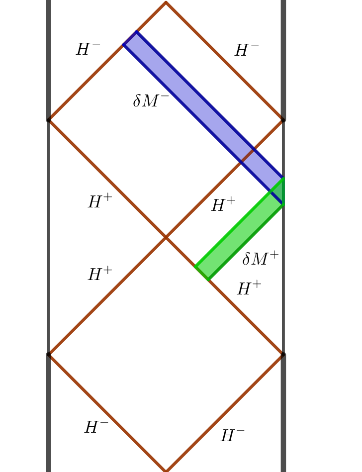
Figure 1: A spacetime diagram of charged accelerating black holes with two killing horizons. $H^{+}$ and $H^{-}$ are the corresponding outer and inner horizons. We show the change of the Wheeler-DeWitt patch, in which we fix the left boundary at $t_{L}\to\infty$ and vary the right boundary

In Fig.1, we show the Penrose diagram of charged accelerating black holes which has two killing horizons. The spacetime is invariant under shift transformation $t_{R}\rightarrow t_{R}-\delta t$, $t_{L}\rightarrow t_{L}+\delta t$. Therefore, we can fix the left boundary time $t_{L}=\infty$ and vary the right boundary time $t_{R}$, i.e., we only need to evaluate the action within the regions $\delta M^{(\pm)}$ to show the late-time complexity growth rate.

III.1 Bulk Contributions

In this subsection, we calculate the contributions from bulk action. This corresponds to bulk region $\delta M^{(\pm)}$. Since we can use the same technology for $\delta M^{(\pm)}$, we will neglect the index $(\pm)$. From Eqs. (4), we have

$$R_{ab}-\frac{1}{4}R_{0}g_{ab}=2F_{a}{}^{c}F_{bc}-\frac{1}{2}\mathcal{F}g_{ab}$$ (16)

The bulk action within region $\delta M^{(\pm)}$ can be written as

$$\begin{aligned} I_{\delta M}&=\frac{1}{16\pi}\int_{\delta M}\star\left(\frac{1}{2}R_{0}-\mathcal{F}\right)\\ &=\frac{1}{16\pi}\delta t\int_{N}\left(\frac{1}{2}R_{0}-\mathcal{F}\right)\star\bm{k}\,,\end{aligned}$$ (17)

in which $k^{a}_{(\pm)}$ is the Killing vector filed of the inner and outer horizons. Considering a killing vector field $k^{a}$ and using the killing equation $\nabla_{a}k_{b}+\nabla_{b}k_{a}=0$, we find

$$\begin{aligned} \nabla_{a}\nabla^{a}k^{b}&=-R^{b}{}_{a}k^{a}\\ &=-\frac{1}{4}R_{0}k^{b}-2T^{b}{}_{a}k^{a}\\ &=-\frac{1}{4}R_{0}k^{b}-2F^{bc}F_{ac}k^{a}+\frac{1}{2}\mathcal{F}k^{b}\,.\end{aligned}$$ (18)

The second term can be written as

$$\begin{aligned} k^{a}F_{ac}F^{bc}&=k^{a}(dA)_{ac}F^{bc}\\ &=F^{bc}\mathcal{L}_{k}A_{c}+F^{bc}\nabla_{c}\Phi\\ &=-\nabla_{a}(\Phi F^{ab})+\Phi\nabla_{a}F^{ab}\end{aligned}$$ (19)

with

$$\begin{aligned} \Phi=-A_{a}k^{a}\,.\end{aligned}$$ (20)

Thus, we have

$$\begin{aligned} 2\nabla_{a}\nabla^{a}k^{b}=-\frac{1}{2}R_{0}k^{b}+4\nabla_{c}(\Phi F^{cb})+\mathcal{F}k^{b}\,.\end{aligned}$$ (21)

Using Eqs. (21), Eq. (17) can be written as

$$\begin{aligned} \left(\frac{1}{2}R_{0}-\mathcal{F}\right)\star\bm{k}=d\star\bm{k}-4d\star(\Phi\bm{F})\,.\end{aligned}$$ (22)

Using the above result, we obtain

$$\begin{aligned} &\frac{16\pi I_{\delta M}}{\delta t}=\int_{N}d\star(d\bm{k}-4\Phi\bm{F})\\ &=\int_{r_{\infty}}\star d\bm{k}-\int_{r_{h}}\star d\bm{k}-4\int_{r_{\infty}}\Phi\star\bm{F}+4\int_{r_{h}}\Phi\star\bm{F}\\ &-\int_{\theta=\epsilon}[\star d\bm{k}-4\star(\Phi\bm{F})]+\int_{\theta=\pi-\epsilon}[\star d\bm{k}-4\star(\Phi\bm{F})]\,.\end{aligned}$$ (23)

It is worth noting that there are two extra terms in the last line of Eqs. (23). This is because the metric has two conical deficits at the north pole ($\theta\rightarrow 0$) and the south pole ($\theta\rightarrow\pi$). When $\theta\rightarrow 0$ or $\theta\rightarrow\pi$, the trace of extrinsic curvature $K\rightarrow\infty$. Therefore, it is nature to consider two boundary surface located at $\theta=\epsilon$ and $\theta=\pi-\epsilon$, where $\epsilon\rightarrow 0$. Then, it is not difficulty to show

$$\begin{aligned} \frac{1}{16\pi}\int_{\theta=\epsilon}\star d\bm{k}&\sim\sin^{2}\epsilon\\ \frac{1}{4\pi}\int_{\theta=\epsilon}\star(\Phi\bm{F})&\sim\sin^{2}\epsilon\,.\end{aligned}$$ (24)

Therefore, conical deficits won’t affect the bulk action’s growth rate.

Using the definition of the black hole entropy, we have

$$\begin{aligned} -\frac{1}{16\pi}\int_{r_{h}}\star d\bm{k}=TS\,.\end{aligned}$$ (25)

Considering $\Phi(r_{h})=\Phi_{H}$ is a constant on the horizon, using the definition of electric charge, we have

$$\begin{aligned} Q=\frac{1}{4\pi}\int\star\bm{F}\,.\end{aligned}$$ (26)

Combing the above result, the late-time growth rate of bulk action becomes

$$\begin{aligned} \lim_{t\to\infty}\frac{dI_{\text{bulk}}}{dt}=\left[\Phi_{H}Q+TS\right]_{+}^{-}\,.\end{aligned}$$ (27)

III.2 Joint Contributions

In this subsection, we will calculate the contribution from the joint term. Without loss of generality, we choose the affine parameter for the null generator $l^{a}$ of the right null surface. Meanwhile, we require $l^{a}$ satisfies $\mathcal{L}_{k}l^{a}=0$. We first focus on the joint point $r=r_{-}$ which is the intersection point of the inner horizon. The inner horizon is generated by the killing vector $k^{a}$ and it satisfies

$$k^{b}\nabla_{b}k^{a}=\kappa k^{a}\,.$$ (28)

Therefore, the affinely null generator on the horizon can be constructed as $\bar{k}^{a}=e^{-\kappa t}k^{a}=e^{-\kappa t}(\frac{\partial}{\partial t})^{a}$. The transformation parameter can be written as

$$\begin{aligned} \eta(t)=\ln\left(-\frac{1}{2}\bar{k}\cdot l\right)=-\kappa t+\ln\left(-\frac{1}{2}k\cdot l\right)\,.\end{aligned}$$ (29)

Using the above relation, the joint contribution at $r=r_{-}$ can be written as

$$\begin{aligned} \frac{dI_{\text{joint}}}{dt}=\frac{1}{8\pi}\frac{d}{dt}\int_{S}d^{2}\theta\sqrt{\sigma}\eta=-\frac{\kappa}{2\pi}S=-T^{(-)}S^{(-)}\,.\end{aligned}$$ (30)

A similar calculation shows the contribution from past meeting point $r=r_{+}$ has the same form. The late-time growth rate of joint contribution is given by

$$\begin{aligned} \lim_{t\rightarrow\infty}\frac{dI_{\text{joint}}}{dt}=T^{(+)}S^{(+)}-T^{(-)}S^{(-)}\,.\end{aligned}$$ (31)

From Eq. (27), we see this term will cancel $TS$ term in bulk contribution.

III.3 Counterterm Contributions

In this subsection, we will evaluate the counterterm contributions. The counterterm contributions can be written as

$$\begin{aligned} I_{\text{ct}}=\frac{1}{8\pi}\int_{N}d\lambda d^{2}\theta\sqrt{\gamma}\Theta\ln(l_{\text{ct}}\Theta)\end{aligned}$$ (32)

We first consider the upper two null segements. The right null segement is generated by $l^{a}$. The left null segement is on inner horizon and we choose the affinely null generator $\bar{k}^{a}=e^{-kt}k^{a}$. In previous subsection, we require the the null generator $l^{a}$ satisfies $\mathcal{L}_{k}l^{a}=0$. It is easy to see $\mathcal{L}_{k}\Theta=0$ for both generators. Therefore, the rate of counterterm contributions vanish.

III.4 Surfaces Contributions

From Eq. (6), we see the metric has two conical deficits at the north pole ($\theta\rightarrow 0$) and south pole ($\theta\rightarrow\pi$). The trace of extrinsic curvature $K\rightarrow\infty$ when $\theta\rightarrow 0$ and $\theta\rightarrow\pi$. Therefore, we should add two extra boundary surfaces at $\theta=\epsilon$ and $\theta=\pi-\epsilon$. The surfaces contributions from $\theta\rightarrow 0$ and $\theta\rightarrow\pi$ is given by

$$\begin{aligned} I_{\Sigma_{\theta}}=\frac{\text{sign}(\sigma)}{8\pi}\int_{\Sigma_{\theta}}\bm{\varpi}\,,\end{aligned}$$ (33)

where $\text{sign}(\sigma)=-1$ for $\theta=\epsilon$, $\text{sign}(\sigma)=-1$ for $\theta=\pi-\epsilon$ and three form $\bm{\varpi}$ can be written as

$$\begin{aligned} \bm{\varpi}=\sqrt{|h|}Kdt\wedge dr\wedge d\phi\,.\end{aligned}$$ (34)

Where $h$ is the determinant of induced metric.

Using the language of differential forms, the above Eq. (33) can be expressed as

$$\begin{aligned} I_{\Sigma_{\theta}}=\delta t\frac{\text{sign}(\sigma)}{8\pi}\int_{\Sigma_{\theta}}\xi\cdot\bm{\varpi}\,.\end{aligned}$$ (35)

From Eq. (6), we find

$$I_{\Sigma_{\theta}}=\frac{\text{sign}(\sigma)\delta t}{8\pi}\int\gamma^{(\pm)}\frac{1}{(1\pm Ar)^{2}}drd\varphi$$ (36)

where $\gamma^{(\pm)}$ is given by

$$\gamma^{(\pm)}=-\sqrt{\frac{(1\pm 2Am+A^{2}q^{2})(1+2Am+A^{2}q^{2})R_{0}}{k^{2}(1+A^{2}q^{2})(12A^{2}+12A^{4}q^{2}+R_{0})}}\,.$$ (37)

Then, at late times, the surfaces contributions can be written as

$$\begin{aligned} I_{\Sigma_{\theta}}=&\frac{\gamma^{(+)}\delta t}{4\pi A}\left(\frac{1}{1+Ar_{-}}-\frac{1}{1+Ar_{+}}\right)\\ &+\frac{\gamma^{(-)}\delta t}{4\pi A}\left(\frac{1}{1-Ar_{+}}-\frac{1}{1-Ar_{-}}\right)\end{aligned}$$ (38)

III.5 Complexity growth rate

Combining all the previous results, the late-time complexity growth rate is given by

$$\begin{aligned} \frac{1}{\pi\hbar}\frac{dC_{A}}{dt}=&\left(\Phi^{(-)}_{H}-\Phi^{(+)}_{H}\right)Q+\frac{\gamma^{(+)}}{4\pi A}\left(\frac{1}{1+Ar_{-}}-\frac{1}{1+Ar_{+}}\right)\\ &+\frac{\gamma^{(-)}}{4\pi A}\left(\frac{1}{1-Ar_{+}}-\frac{1}{1-Ar_{-}}\right)\,.\end{aligned}$$ (39)

This result is different from the ordinary charged systems. For the ordinary charged systems, it has been shown that the late-time growth rate is $\Phi_{H}^{(-)}Q-\Phi_{H}^{(+)}Q$. Because of the conical deficits, there are some extra terms that are evaluated on the inner and outer horizons.

IV Conclusion

In this paper, we considered the charged accelerating black holes which have two conical deficits on the north and south poles in Einstein-Maxwell theory. From the perspective of AdS/CFT, the dual bound system of this bulk gravity also has two conical deficits on the north and south poles. To investigate the influence of the conical deficits on the complexity of the boundary system, we evaluated the growth rate of the CA complexity in charged accelerating black holes. We show that the time-time complexity growth rate is different from the result Eq. (2) of an ordinary charged system. There is an additional term that is evaluated on the inner and outer horizons. These imply that the complexity can reflect some information of conical deficits in the boundary CFT system.

V Acknowledgments

This research was supported by NSFC Grants No. 11775022 and 11873044.

References

- (1) L. Susskind, Fortsch. Phys. 64 (2016), 24-43 doi:10.1002/prop.201500092 [arXiv:1403.5695 [hep-th]].
- (2) S. Aaronson, [arXiv:1607.05256 [quant-ph]].
- (3) D. Stanford and L. Susskind, Phys. Rev. D 90 (2014) no.12, 126007 doi:10.1103/PhysRevD.90.126007 [arXiv:1406.2678 [hep-th]].
- (4) A. R. Brown, D. A. Roberts, L. Susskind, B. Swingle and Y. Zhao, Phys. Rev. Lett. 116 (2016) no.19, 191301 doi:10.1103/PhysRevLett.116.191301 [arXiv:1509.07876 [hep-th]].
- (5) A. R. Brown, D. A. Roberts, L. Susskind, B. Swingle and Y. Zhao, Phys. Rev. D 93 (2016) no.8, 086006 doi:10.1103/PhysRevD.93.086006 [arXiv:1512.04993 [hep-th]].
- (6) D. A. Roberts, D. Stanford and L. Susskind, JHEP 03 (2015), 051 doi:10.1007/JHEP03(2015)051 [arXiv:1409.8180 [hep-th]].
- (7) L. Lehner, R. C. Myers, E. Poisson and R. D. Sorkin, Phys. Rev. D 94 (2016) no.8, 084046 doi:10.1103/PhysRevD.94.084046 [arXiv:1609.00207 [hep-th]].
- (8) R. Jefferson and R. C. Myers, JHEP 10 (2017), 107 doi:10.1007/JHEP10(2017)107 [arXiv:1707.08570 [hep-th]].
- (9) D. Carmi, R. C. Myers and P. Rath, JHEP 03 (2017), 118 doi:10.1007/JHEP03(2017)118 [arXiv:1612.00433 [hep-th]].
- (10) S. Chapman, M. P. Heller, H. Marrochio and F. Pastawski, Phys. Rev. Lett. 120 (2018) no.12, 121602 doi:10.1103/PhysRevLett.120.121602 [arXiv:1707.08582 [hep-th]].
- (11) D. Carmi, S. Chapman, H. Marrochio, R. C. Myers and S. Sugishita, JHEP 11 (2017), 188 doi:10.1007/JHEP11(2017)188 [arXiv:1709.10184 [hep-th]].
- (12) P. Caputa, N. Kundu, M. Miyaji, T. Takayanagi and K. Watanabe, JHEP 11 (2017), 097 doi:10.1007/JHEP11(2017)097 [arXiv:1706.07056 [hep-th]].
- (13) S. Chapman, H. Marrochio and R. C. Myers, JHEP 01 (2017), 062 doi:10.1007/JHEP01(2017)062 [arXiv:1610.08063 [hep-th]].
- (14) A. R. Brown and L. Susskind, Phys. Rev. D 97 (2018) no.8, 086015 doi:10.1103/PhysRevD.97.086015 [arXiv:1701.01107 [hep-th]].
- (15) M. Guo, Z. Y. Fan, J. Jiang, X. Liu and B. Chen, Phys. Rev. D 101, no.12, 126007 (2020) doi:10.1103/PhysRevD.101.126007 [arXiv:2004.00344 [hep-th]].
- (16) Z. Y. Fan and M. Guo, Nucl. Phys. B 950, 114818 (2020) doi:10.1016/j.nuclphysb.2019.114818 [arXiv:1811.01473 [hep-th]].
- (17) Z. Y. Fan and M. Guo, JHEP 08, 031 (2018) [erratum: JHEP 09, 121 (2019)] doi:10.1007/JHEP08(2018)031 [arXiv:1805.03796 [hep-th]].
- (18) J. Couch, W. Fischler and P. H. Nguyen, JHEP 03 (2017), 119 doi:10.1007/JHEP03(2017)119 [arXiv:1610.02038 [hep-th]].
- (19) R. G. Cai, S. M. Ruan, S. J. Wang, R. Q. Yang and R. H. Peng, JHEP 09 (2016), 161 doi:10.1007/JHEP09(2016)161 [arXiv:1606.08307 [gr-qc]].
- (20) L. Susskind and Y. Zhao, [arXiv:1408.2823 [hep-th]].
- (21) D. A. Roberts and B. Yoshida, JHEP 04 (2017), 121 doi:10.1007/JHEP04(2017)121 [arXiv:1610.04903 [quant-ph]].
- (22) O. Ben-Ami and D. Carmi, JHEP 11 (2016), 129 doi:10.1007/JHEP11(2016)129 [arXiv:1609.02514 [hep-th]].
- (23) R. Khan, C. Krishnan and S. Sharma, Phys. Rev. D 98 (2018) no.12, 126001 doi:10.1103/PhysRevD.98.126001 [arXiv:1801.07620 [hep-th]].
- (24) L. Hackl and R. C. Myers, JHEP 07 (2018), 139 doi:10.1007/JHEP07(2018)139 [arXiv:1803.10638 [hep-th]].
- (25) S. Chapman, H. Marrochio and R. C. Myers, JHEP 06 (2018), 046 doi:10.1007/JHEP06(2018)046 [arXiv:1804.07410 [hep-th]].
- (26) S. Chapman, J. Eisert, L. Hackl, M. P. Heller, R. Jefferson, H. Marrochio and R. C. Myers, SciPost Phys. 6 (2019) no.3, 034 doi:10.21468/SciPostPhys.6.3.034 [arXiv:1810.05151 [hep-th]].
- (27) R. Q. Yang, C. Niu, C. Y. Zhang and K. Y. Kim, JHEP 02 (2018), 082 doi:10.1007/JHEP02(2018)082 [arXiv:1710.00600 [hep-th]].
- (28) A. R. Brown, L. Susskind and Y. Zhao, Phys. Rev. D 95 (2017) no.4, 045010 doi:10.1103/PhysRevD.95.045010 [arXiv:1608.02612 [hep-th]].
- (29) A. Reynolds and S. F. Ross, Class. Quant. Grav. 34 (2017) no.10, 105004 doi:10.1088/1361-6382/aa6925 [arXiv:1612.05439 [hep-th]].
- (30) C. A. Agón, M. Headrick and B. Swingle, JHEP 02 (2019), 145 doi:10.1007/JHEP02(2019)145 [arXiv:1804.01561 [hep-th]].
- (31) S. Chapman, H. Marrochio and R. C. Myers, JHEP 06 (2018), 114 doi:10.1007/JHEP06(2018)114 [arXiv:1805.07262 [hep-th]].
- (32) P. Caputa and J. M. Magan, Phys. Rev. Lett. 122 (2019) no.23, 231302 doi:10.1103/PhysRevLett.122.231302 [arXiv:1807.04422 [hep-th]].
- (33) R. Abt, J. Erdmenger, H. Hinrichsen, C. M. Melby-Thompson, R. Meyer, C. Northe and I. A. Reyes, Fortsch. Phys. 66 (2018) no.6, 1800034 doi:10.1002/prop.201800034 [arXiv:1710.01327 [hep-th]].
- (34) K. Hashimoto, N. Iizuka and S. Sugishita, Phys. Rev. D 96 (2017) no.12, 126001 doi:10.1103/PhysRevD.96.126001 [arXiv:1707.03840 [hep-th]].
- (35) M. Guo, J. Hernandez, R. C. Myers and S. M. Ruan, JHEP 10 (2018), 011 doi:10.1007/JHEP10(2018)011 [arXiv:1807.07677 [hep-th]].
- (36) A. Bhattacharyya, P. Caputa, S. R. Das, N. Kundu, M. Miyaji and T. Takayanagi, JHEP 07 (2018), 086 doi:10.1007/JHEP07(2018)086 [arXiv:1804.01999 [hep-th]].
- (37) M. Alishahiha, A. Faraji Astaneh, A. Naseh and M. H. Vahidinia, JHEP 05 (2017), 009 doi:10.1007/JHEP05(2017)009 [arXiv:1702.06796 [hep-th]].
- (38) M. Alishahiha, A. Faraji Astaneh, M. R. Mohammadi Mozaffar and A. Mollabashi, JHEP 07 (2018), 042 doi:10.1007/JHEP07(2018)042 [arXiv:1802.06740 [hep-th]].
- (39) B. Swingle and Y. Wang, JHEP 09 (2018), 106 doi:10.1007/JHEP09(2018)106 [arXiv:1712.09826 [hep-th]].
- (40) R. G. Cai, M. Sasaki and S. J. Wang, Phys. Rev. D 95 (2017) no.12, 124002 doi:10.1103/PhysRevD.95.124002 [arXiv:1702.06766 [gr-qc]].
- (41) A. Bhattacharyya, A. Shekar and A. Sinha, JHEP 10 (2018), 140 doi:10.1007/JHEP10(2018)140 [arXiv:1808.03105 [hep-th]].
- (42) R. Q. Yang, Phys. Rev. D 97 (2018) no.6, 066004 doi:10.1103/PhysRevD.97.066004 [arXiv:1709.00921 [hep-th]].
- (43) A. Belin, A. Lewkowycz and G. Sárosi, JHEP 03 (2019), 044 doi:10.1007/JHEP03(2019)044 [arXiv:1811.03097 [hep-th]].
- (44) Y. S. An and R. H. Peng, Phys. Rev. D 97 (2018) no.6, 066022 doi:10.1103/PhysRevD.97.066022 [arXiv:1801.03638 [hep-th]].
- (45) Z. Fu, A. Maloney, D. Marolf, H. Maxfield and Z. Wang, JHEP 02 (2018), 072 doi:10.1007/JHEP02(2018)072 [arXiv:1801.01137 [hep-th]].
- (46) B. Chen, W. M. Li, R. Q. Yang, C. Y. Zhang and S. J. Zhang, JHEP 07 (2018), 034 doi:10.1007/JHEP07(2018)034 [arXiv:1803.06680 [hep-th]].
- (47) J. L. F. Barbon and E. Rabinovici, JHEP 01 (2016), 084 doi:10.1007/JHEP01(2016)084 [arXiv:1509.09291 [hep-th]].
- (48) B. Czech and L. Lamprou, Phys. Rev. D 90 (2014), 106005 doi:10.1103/PhysRevD.90.106005 [arXiv:1409.4473 [hep-th]].
- (49) R. Q. Yang, Y. S. An, C. Niu, C. Y. Zhang and K. Y. Kim, Eur. Phys. J. C 79 (2019) no.2, 109 doi:10.1140/epjc/s10052-019-6600-3 [arXiv:1803.01797 [hep-th]].
- (50) T. Takayanagi, JHEP 12 (2018), 048 doi:10.1007/JHEP12(2018)048 [arXiv:1808.09072 [hep-th]].
- (51) L. Susskind, Fortsch. Phys. 64 (2016), 84-91 doi:10.1002/prop.201500091 [arXiv:1507.02287 [hep-th]].
- (52) R. Q. Yang, C. Niu and K. Y. Kim, JHEP 09 (2017), 042 doi:10.1007/JHEP09(2017)042 [arXiv:1701.03706 [hep-th]].
- (53) P. A. Cano, R. A. Hennigar and H. Marrochio, Phys. Rev. Lett. 121 (2018) no.12, 121602 doi:10.1103/PhysRevLett.121.121602 [arXiv:1803.02795 [hep-th]].
- (54) X. L. Qi and A. Streicher, JHEP 08 (2019), 012 doi:10.1007/JHEP08(2019)012 [arXiv:1810.11958 [hep-th]].
- (55) A. Reynolds and S. F. Ross, Class. Quant. Grav. 34 (2017) no.17, 175013 doi:10.1088/1361-6382/aa8122 [arXiv:1706.03788 [hep-th]].
- (56) T. Ali, A. Bhattacharyya, S. Shajidul Haque, E. H. Kim and N. Moynihan, JHEP 04 (2019), 087 doi:10.1007/JHEP04(2019)087 [arXiv:1810.02734 [hep-th]].
- (57) J. Couch, S. Eccles, W. Fischler and M. L. Xiao, JHEP 03 (2018), 108 doi:10.1007/JHEP03(2018)108 [arXiv:1710.07833 [hep-th]].
- (58) D. W. F. Alves and G. Camilo, JHEP 06 (2018), 029 doi:10.1007/JHEP06(2018)029 [arXiv:1804.00107 [hep-th]].
- (59) H. Huang, X. H. Feng and H. Lu, Phys. Lett. B 769 (2017), 357-361 doi:10.1016/j.physletb.2017.04.011 [arXiv:1611.02321 [hep-th]].
- (60) W. D. Guo, S. W. Wei, Y. Y. Li and Y. X. Liu, Eur. Phys. J. C 77 (2017) no.12, 904 doi:10.1140/epjc/s10052-017-5466-5 [arXiv:1703.10468 [gr-qc]].
- (61) A. P. Reynolds and S. F. Ross, Class. Quant. Grav. 35 (2018) no.9, 095006 doi:10.1088/1361-6382/aab32d [arXiv:1712.03732 [hep-th]].
- (62) W. J. Pan and Y. C. Huang, Phys. Rev. D 95 (2017) no.12, 126013 doi:10.1103/PhysRevD.95.126013 [arXiv:1612.03627 [hep-th]].
- (63) Z. Y. Fan and M. Guo, Phys. Rev. D 100 (2019), 026016 doi:10.1103/PhysRevD.100.026016 [arXiv:1903.04127 [hep-th]].
- (64) J. Jiang, Phys. Rev. D 98 (2018) no.8, 086018 doi:10.1103/PhysRevD.98.086018 [arXiv:1810.00758 [hep-th]].
- (65) J. F. Plebanski and M. Demianski, Annals Phys. 98 (1976), 98-127 doi:10.1016/0003-4916(76)90240-2
- (66) M. Zhang and R. B. Mann, Phys. Rev. D 100 (2019) no.8, 084061 doi:10.1103/PhysRevD.100.084061 [arXiv:1908.05118 [hep-th]].
- (67) M. Zhang and R. B. Mann, Phys. Rev. D 100 (2019) no.8, 084061 doi:10.1103/PhysRevD.100.084061 [arXiv:1908.05118 [hep-th]].