Wavelet-Packets for Deepfake Image Analysis and Detection

Abstract

As neural networks become able to generate realistic artificial images, they have the potential to improve movies, music, video games and make the internet an even more creative and inspiring place. Yet, the latest technology potentially enables new digital ways to lie. In response, the need for a diverse and reliable method toolbox arises to identify artificial images and other content. Previous work primarily relies on pixel-space cnn or the Fourier transform. Synthesized fake image analysis and detection methods based on a multi-scale wavelet representation, localized in both space and frequency, have been absent thus far. The wavelet transform conserves spatial information to a degree, allowing us to present a new analysis. Comparing the wavelet coefficients of real and fake images significant differences are identified, where this representation also allows further interpretations. Additionally, this paper proposes to learn a model for the detection of synthetic images based on the wavelet-packet representation of natural and gan-generated images. Our forensic classifiers exhibit competitive or improved performance at small network sizes, as we demonstrate on the ffhq, celeba and lsun source identification problems. Furthermore, we study the binary ffpp fake-detection problem.

1 Introduction

While gan can extract useful representations from data, translate textual descriptions into images, transfer scene and style information between images or detect objects (Gui et al.,, 2022), they can also enable abusive actors to quickly and easily generate potentially damaging, highly realistic fake images, colloquially called deepfakes (Parkin,, 2012; Frank et al.,, 2020). As the internet becomes a more prominent virtual public space for political discourse and social media outlet (Applebaum,, 2020), deepfakes present a looming threat to its integrity that must be met with techniques for differentiating the real and trustworthy from the fake.

Previous algorithmic techniques for separating real from computer-hallucinated images of people have relied on identifying fingerprints in either the spatial (Yu et al.,, 2019; Marra et al.,, 2019) or frequency (Frank et al.,, 2020; Dzanic et al.,, 2020) domain. However, to the best of our knowledge, no techniques have jointly considered the two domains in a multi-scale fashion, for which we propose to employ wavelet-packet coefficients representing a spatio-frequency representation.

In this paper, we make the following contributions:

• We present a wavelet-packet-based analysis of gan-generated images. Compared to existing work in the frequency domain, we examine the spatio-frequency properties of gan-generated content for the first time. We find differences between real and synthetic images in both the wavelet-packet mean and standard deviation, with increasing frequency and at the edges. The differences in mean and standard deviation also holds between different sources of synthetic images.

• To the best of our knowledge, we present the first application and implementation of boundary wavelets for image analysis in the deep learning context. Proper implementation of boundary-wavelet filters allows us to share identical network architectures across different wavelet lengths.

• As a result of the aforementioned wavelet-packet-based analysis, we build classifiers to identify image sources. We work with fixed seed values for reproducibility and report mean and standard deviations over five runs whenever possible. Our systematic analysis shows improved or competitive performance.

• Integrating existing Fourier-based methods, we introduce fusion networks combining both approaches. Our best networks outperform previous purely Fourier or pixel-based approaches on the CelebA and Lsun bedrooms benchmarks. Both benchmarks have been previously studied in Yu et al., (2019) and Frank et al., (2020).

We believe our virtual public spaces and social media outlets will benefit from a growing, diverse toolbox of techniques enabling automatic detection of gan-generated content, where the introduced wavelet-based approach provides a competitive and interpretable addition. The source code for our wavelet toolbox, the first publicly available toolbox for fast boundary-wavelet transforms in the python world, and our experiments is available at https://github.com/v0lta/PyTorch-Wavelet-Toolbox and https://github.com/gan-police/frequency-forensics.

2 Motivation

“Wavelets are localized waves. Instead of oscillating forever, they drop to zero.” Strang and Nguyen, (1996). This important observation explains why wavelets allow us to conserve some spatio-temporal relations. The Fourier transform uses sine and cosine waves, which never stop fluctuating. Consequently, Fourier delivers an excellent frequency resolution while losing all spatio-temporal information. We want to learn more about the spatial organization of differences in the frequency domain, which is our first motivation to work with wavelets.

The second part of our motivation lies in the representation power of wavelets. Images often contain sharp borders where pixel values change rapidly. Monochromatic areas are also common, where the signal barely changes at all. Sharp borders or steps are hard to represent in the Fourier space. As the sine and cosine waves do not fit well, we observe the Gibbs-phenomenon (Strang and Nguyen,, 1996) as high-frequency coefficients pollute the spectrum. For a dull, flat region, Fourier requires an infinite sum (Van den Berg,, 2004). The Fourier transform is uneconomical in these two cases. Furthermore, the fast wavelet transform can be used with many different wavelets. Having a choice that allows us to explore and choose a basis which suits our needs is our second motivation to work with wavelets.

Before discussing the mechanics of the fwt and its packet variant, we present a proof of concept experiment in Figure 1. We investigate the coefficients of the level 3 Haar wavelet packet transform. Computations use 5k $1024\times 1024$ pixel images from ffhq and 5k $1024\times 1024$ pixel images generated by StyleGAN.

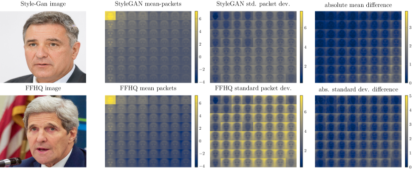
Figure 1: This figure compares single time-domain images and absolute $\ln$-scaled mean wavelet packets and their standard deviations. The first column shows two example images, the second mean packets, the third standard deviations, and the fourth mean and standard deviation differences. Mean values and standard deviations have been computed on 5k $1024\times 1024$ ffhq- and StyleGAN-generated images each. The order of the packets has the frequency increasing from the top left to the bottom right. We observe significant differences. The mean is significantly different for higher frequencies and at image edges. The standard deviations differ in the background across the entire spectrum. In the supplementary, Figure 22 shows the exact filter sequences for each packet. Best viewed in color.

The leftmost columns of Figure 1 show a sample from both ffhq and a StyleGAN generated one. Mean wavelet packets appear in the second, and their standard deviation in the third column. Finally, the rightmost column plots the absolute mean packets and standard deviation differences. For improved visibility, we rescale the absolute values of the packet representation, averaged first over the three color bands, using the ln.

We find that the mean wavelet packets of gan-generated images are often significantly brighter. The differences become more pronounced as the frequency increases from the top left to the bottom right. The differences in high-frequency packets independently confirm Dzanic et al., (2020), who saw the most significant differences for high-frequency Fourier-coefficients.

The locality of the wavelet filters allows face-like shapes to appear, but the image edges stand out, allowing us to pinpoint the frequency disparities. We now have an intuition regarding the local origin of the differences. We note that Haar wavelet packets do not use padding or orthogonalization and conclude that the differences stem from gan generation. For the standard deviations, the picture is reversed. Instead of the GAN the ffhq-packets appear brighter. The StyleGAN packets do not deviate as much as the data in the original data set. The observation suggests that the gan did not capture the complete variance of the original data. Our evidence indicates that gan-generated backgrounds are of particular monotony across all frequency bands.

In the next sections, we survey related work and discuss how the fwt and wavelet packets in Figure 1 are computed.

3 Related work

3.1 Generative adversarial networks

The advent of gan (Goodfellow et al.,, 2014) heralded several successful image generation projects. We highlight the contribution of the progressive growth technique, in which a small network is trained on smaller images then gradually increased in complexity/number of weights and image size, on the ability of optimization to converge at high resolutions of $1024\times 1024$ pixels (Karras et al.,, 2018). As a supplement, style transfer methods (Gatys et al.,, 2016) have been integrated into new style-based generators. The resulting style-gan have increased the statistical variation of the hallucinated faces (Karras et al.,, 2019, 2020). Finally, regularization (e.g., using spectral methods) has increased the stability of the optimization process (Miyato et al.,, 2018). The recent advances have allowed large-scale training (Brock et al.,, 2019), which in turn improves the quality further.

Conditional methods allow to partially manipulate images, Antipov et al., (2017) for example proposes to use conditional gan for face aging. Similarly, gan allow the transfer of facial expressions (Deepfake-Faceswap-Contributors,, 2018; Thies et al.,, 2019), an ability of particular importance from a detection point of view. For a recent exhaustive review on gan theory, architecture, algorithms, and applications, we refer to Gui et al., (2022).

3.2 Diffusion Probabilistic Models

As an alternative class of approaches to gan, recently, two closely related probabilistic generative models, diffusion (probabilistic) models and score-based generative models, respectively, were shown to produce high-quality images, see Ho et al., (2020); Dhariwal and Nichol, (2021); Song et al., (2021) and their references. In short, images are generated by reversing in the sampling phase a gradual noising process used during training. Further, Dhariwal and Nichol, (2021) proposes to use gradients from a classifier to guide a diffusion model during sampling, with the aim to trade-off diversity for fidelity.

3.3 Deepfake detection

Deepfake detectors broadly fall into two categories. The first group works in the frequency domain. Projects include the study of natural and deep network generated images in the frequency space created by the dct, as well as detectors based on Fourier features (Zhang et al.,, 2019; Durall et al.,, 2019; Dzanic et al.,, 2020; Frank et al.,, 2020; Durall et al.,, 2020; Giudice et al.,, 2021), these provide frequency space information, but the global nature of these bases means all spatial relations are missing. In particular, Frank et al., (2020) visualizes the dct transformed images and identifies artifacts created by different upsampling methods. We learn that the transformed images are efficient classification features, which allow significant parameter reductions in GAN identification classifiers. Instead of relying on the dct, Dzanic et al., (2020) studied the distribution of Fourier coefficients for real and gan-generated images. After noting significant deviations of the mean frequencies for gan generated- and real-images, classifiers are trained. Similarly, Giudice et al., (2021) studies statistics of the dct coefficients and uses estimations for each GAN-engine for classification. Dzanic et al., (2020) found high-frequency discrepancies for GAN-generated imagery, built detectors, and spoofed the newly trained Fourier classifiers by manually adapting the coefficients in Fourier-space. Finally, He et al., (2021) combined 2d-FFT and DCT features and observed improved performance.

The second group of classifiers works in the spatial or pixel domain, among others, (Yu et al.,, 2019; Wang et al., 2020a, ; Wang et al., 2020b, ; Zhao et al., 2021a, ; Zhao et al., 2021b, ) train (convolutional) neural networks directly on the raw images to identify various gan architectures. Building upon pixel-CNN Wang and Deng, (2021) adds neural attention. According to (Yu et al.,, 2019), the classifier features in the final layers constitute the fingerprint for each gan and are interesting to visualize. Instead of relying on deep-learning, (Marra et al.,, 2019) proposed gan-fingerprints working exclusively with denoising-filter and mean operations, whereas (Guarnera et al.,, 2020) computes convolutional traces.

Tang et al., (2021) uses a simple first-level discrete wavelet transform, this means no multi-scale representation as a preprocessing step to compute spectral correlations between the color bands of an image, which are then further processed to obtain features for a classifier. Younus and Hasan, (2020) use a Haar-wavelet transform to study edge inconsistencies in manipulated images.

To the best of our knowledge, we are the first to work directly with a spatio-frequency wavelet packet representation in a multi-scale fashion. Our analysis goes beyond previous Fourier-based studies. Fourier loses all spatial information while wavelets preserve it. Compared to previous wavelet-based work, we also consider the packet approach and boundary wavelets. The packet approach allows us to decompose high-frequency bands in fine detail. Boundary wavelets enable us to work with higher-level wavelets, which the machine learning literature has largely ignored thus far. As we demonstrate in the next section, wavelet packets allow visualization of frequency information while, at the same time, preserving local information.

Previously proposed deepfake detectors had to detect fully (Frank et al.,, 2020) or partially (Rossler et al.,, 2019) faked images. In this paper we do both. Sections 5.1, 5.2 and 5.3 consider complete fakes and section 5.4 studies detection of partial neural fakes. Additionally we examine images generated by guided diffusion (Dhariwal and Nichol,, 2021) in section 5.5. We demonstrate our ability to identify images from this source by training a forensic classifier. A recent survey on deepfake generation and detection can be found in Zhang, (2022).

3.4 Wavelets

Originally developed within applied mathematics (Mallat,, 1989; Daubechies,, 1992), wavelets are a long-established part of the image analysis and processing toolbox (Taubman and Marcellin,, 2002; Strang and Nguyen,, 1996; Jensen and la Cour-Harbo,, 2001). In the world of traditional image coding, wavelet-based codes have been developed to replace techniques based on the dct (Taubman and Marcellin,, 2002). Early applications of wavelets in machine learning studied the integration of wavelets into neural networks for function learning (Zhang et al.,, 1995). Within this line of work, wavelets have previously served as input features (Chen et al.,, 2015), or as early layers of scatter nets (Mallat,, 2012; Cotter,, 2020). Deeper inside neural networks, wavelets have appeared within pooling layers using static Haar (Wang et al., 2020c, ; Williams and Li,, 2018) or adaptive wavelets (Wolter and Garcke,, 2021; Ha et al.,, 2021). Within the subfield of generative networks, concurrent research (Gal et al.,, 2021) explored the use of Haar-wavelets to improve gan generated image content. Bruna and Mallat, (2013) and Oyallon and Mallat, (2015) found that fixed wavelet filters in early convolution layers can lead to performance similar to trained neural networks. The resulting architectures are known as scatter nets. This paper falls into a similar line of work by building neural network classifiers on top of wavelet packets. We find this approach is particularly efficient in limited training data scenarios. Section 5.2.1 discusses this observation in detail.

The machine learning literature often limits itself to the Haar wavelet (Wang et al., 2020c, ; Williams and Li,, 2018; Gal et al.,, 2021). Perhaps because it is padding-free and does not require boundary value treatment. The following sections will explain the fwt and how to work with longer wavelets effectively.

4 Methods

In this section, we briefly present the nuts and bolts of the fast wavelet transform and its packet variant. For multi-channel color images, we transform each color separately. For simplicity, we will only consider single channels in the following exposition.

4.1 The fwt

fwt (Mallat,, 1989; Daubechies,, 1992; Strang and Nguyen,, 1996; Jensen and la Cour-Harbo,, 2001; Mallat,, 2009) utilize convolutions to decompose an input signal into its frequency components. Repeated applications of the wavelet transform result in a multi-scale analysis. Convolution is here a linear operation and linear operations are often written in matrix form. Consequently, we aim to find a matrix that allows the computation of the fast wavelet transform (Strang and Nguyen,, 1996):

$$\mathbf{b}=\mathbf{A}\mathbf{x}.$$ (1)

$\mathbf{A}$ is a product of multiple scale-matrices. The non-zero elements in $\mathbf{A}$ are populated with the coefficients from the selected filter pair. Given the wavelet filter degree $d$, each filter has $N=2d$ coefficients. Repeating diagonals compute convolution operations with the so-called analysis filter vector pair $\mathbf{f}_{\mathcal{L}}$ and $\mathbf{f}_{\mathcal{H}}$, where the filters are arranged as vectors in $\mathbb{R}^{N}$. The subscripts $\mathcal{L}$ denote the one-dimensional low-pass and $\mathcal{H}$ the high pass filter, respectively. The filter pair appears within the diagonal patterns of the stride two convolution matrices $\mathbf{H}_{\mathcal{L}}$ and $\mathbf{H}_{\mathcal{H}}$. Overall one observes the pattern (Strang and Nguyen,, 1996)

$$\mathbf{A}=\dots\begin{pmatrix}\begin{array}[]{c|c}\mathbf{H}_{\mathcal{L}}&\\ \mathbf{H}_{\mathcal{H}}&\\ \hline\cr&\mathbf{I}\\ \end{array}\end{pmatrix}\begin{pmatrix}\mathbf{H}_{\mathcal{L}}\\ \mathbf{H}_{\mathcal{H}}\end{pmatrix}.$$ (2)

The equation describes the first two FWT-matrices. Instead of the dots, we can imagine additional analysis matrices. The analysis matrix $\mathbf{A}$ records all operations by matrix multiplication.

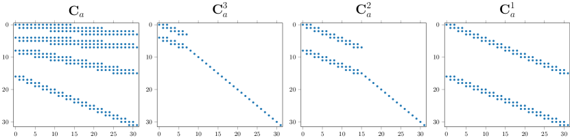
Figure 2: Truncated single-dimensional analysis convolution matrices for a signal of length 32 using for example a Daubechies-two wavelet. The decomposition level increases from right to left. On the leftmost side the product of the first three is shown. We are looking at truncated versions of the infinite matrices described by equation (2). The title reads $\mathbf{C}_{a}$ because the analysis convolution matrix is different from the wavelet matrix, which we discuss further in section 4.3 on boundary filters.

In Figure 2 we illustrate a level three transform, where we see equation (2) at work. Ideally, $\mathbf{A}$ is infinitely large and orthogonal. For finite signals, the ideal matrices have to be truncated. $\mathbf{C}$ denotes finite length untreated convolution matrices, subscript $a$ and $s$ mark analysis, and transposed synthesis convolutions. Second-degree wavelet coefficients from four filters populate the convolution matrices. The identity tail of the individual matrices grows as scales complete. The final convolution matrix is shown on the left. Supplementary section 9.3 presents the construction of the synthesis matrices, which undo the analysis steps.

Common choices for 1D wavelets are the Daubechies-wavelets (“db”) and their less asymmetrical variant, the symlets (“sym”). We refer the reader to supplementary section 9.2 or Mallat, (2009) for an in-depth discussion. Note that the fwt is invertible, to construct the synthesis matrix $\mathbf{S}$ for $\mathbf{S}\mathbf{A}~{}=~{}\mathbf{I}$, we require the synthesis filter pair $\mathbf{f}_{\mathcal{L}},\mathbf{f}_{\mathcal{H}}$. The filter coefficients populate transposed convolution matrices. Details are discussed in supplementary section 9.3. To ensure the transform is invertible and visualizations interpretable, not just any filter will do. The perfect reconstruction and anti-aliasing conditions must hold. We briefly present these two in supplementary section 9.1 and refer to Strang and Nguyen, (1996) and Jensen and la Cour-Harbo, (2001) for an excellent further discussion of these conditions.

4.2 The two-dimensional wavelet transform

To extend the single-dimensional case to two-dimensions, one dimensional wavelet pairs are often transformed. Outer products allow us to obtain two dimensional quadruples from single dimensional filter pairs (Vyas et al.,, 2018):

$$\mathbf{f}_{a} =\mathbf{f}_{\mathcal{L}}\mathbf{f}_{\mathcal{L}}^{T}, \mathbf{f}_{h} =\mathbf{f}_{\mathcal{L}}\mathbf{f}_{\mathcal{H}}^{T}, \mathbf{f}_{v} =\mathbf{f}_{\mathcal{H}}\mathbf{f}_{\mathcal{L}}^{T}, \mathbf{f}_{d} =\mathbf{f}_{\mathcal{H}}\mathbf{f}_{\mathcal{H}}^{T}.$$ (3)

In the equations above, $\mathbf{f}$ denotes a filter vector. In the two-dimensional case, a denotes the approximation coefficients, h denotes the horizontal coefficients, v denotes vertical coefficients, and d denotes the diagonal coefficients. The 2D transformation at representation level $q+1$ requires the input $\mathbf{x}_{q}$ as well as a filter quadruple $\mathbf{f}_{k}$ for $k\in[a,h,v,d]$ and is computed by

$$\mathbf{x}_{q}*\mathbf{f}_{k}=\mathbf{k}_{q+1},$$ (4)

where $*$ denotes stride two convolution. Note the input image is at level zero, i.e.  $\mathbf{x}_{0}=\mathbf{I}$, while for stage $q$ the low pass result of $q-1$ is used as input.

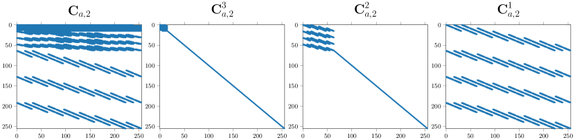
Figure 3: Two dimensional analysis convolution matrix sparsity patterns. The first three matrices from the right are individual convolution matrices. The matrix on the very left is the combined sparse convolution matrix.

The two dimensional transform is also linear and can therefore be expressed in matrix form:

$$\mathbf{A}_{2d}=\dots\begin{pmatrix}\begin{array}[]{c|c}\mathbf{H}_{a}&\\ \mathbf{H}_{h}&\\ \mathbf{H}_{v}&\\ \mathbf{H}_{d}&\\ \hline\cr&\mathbf{I}\\ \end{array}\end{pmatrix}\begin{pmatrix}\mathbf{H}_{a}&\\ \mathbf{H}_{h}&\\ \mathbf{H}_{v}&\\ \mathbf{H}_{d}&\\ \end{pmatrix}.$$ (5)

Similarly to the single dimensional case $\mathbf{H}_{k}$ denotes a stride two, two dimensional convolution matrix. We write the inverse or synthesis operation as $\mathbf{F}_{k}$. Figure 3 illustrates the sparsity patterns of the resulting two-dimensional convolution matrices.

4.3 Boundary wavelets

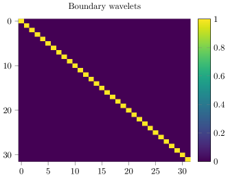
Figure 4: The effect of boundary wavelet treatment. Single-dimensional Transformation-Matrices of shape 32 by 32 are constructed. The plot on the left shows the element-wise absolute values of $\mathbf{C_{s}}\cdot\mathbf{C_{a}}$. The right plot shows the element-wise absolute values of $\mathbf{S}\cdot\mathbf{A}$ for orthogonalized analysis and synthesis matrices. The identity matrix indicates that our matrices have been correctly assembled.

So far, we have described the wavelet transform without considering the finite size of the images. For example, the simple Haar wavelets can be used without modifications in such a case. But, for the transform to preserve all information and be invertible, higher-order wavelets require modifications at the boundary (Strang and Nguyen,, 1996). There are different ways to handle the boundary, including zero-padding, symmetrization, periodic extension, and specific filters on the boundary. The disadvantage of zero-padding or periodic extensions is that discontinuities are artificially created at the border. With symmetrization, discontinuities of the first derivative arise at the border (Jensen and la Cour-Harbo,, 2001). For large images, the boundary effects might be negligible. However, for the employed multi-scale approach of wavelet-packets, as introduced in the next subsection, the artifacts become too severe. Furthermore, zero-padding increases the number of coefficients, which in our application would need different neural network architectures per wavelet. Therefore we employ special boundary filters in the form of the so-called Gram-Schmidt boundary filters (Jensen and la Cour-Harbo,, 2001).

The idea is now to replace the filters at the boundary with specially constructed, shorter filters that preserve both the length and the perfect reconstruction property or other properties of the wavelet transform. We illustrate the impact of the procedure in Figure 4. The product of the untreated convolution matrices appears on the left. The boundary wavelet matrices $\mathbf{S}\cdot\mathbf{A}$ on the right. Appendix Figures 17 and 18 illustrate the sparsity patterns of the resulting sparse analysis and synthesis matrices for the Daubechies two case in 2D.

4.4 Wavelet packets

Presuming to find the essential information in the lower frequencies, note that standard wavelet transformations decompose only the low-pass or $a$ coefficients further. The $h$, $v$, and $d$ coefficients are left untouched. While this is often a reasonable assumption (Strang and Nguyen,, 1996), previous work (Dzanic et al.,, 2020; Schwarz et al.,, 2021) found higher frequencies equally relevant for deepfake detection. For this analysis the wavelet tree will consequently be extended on both the low and high frequency sides. This approach is known as wavelet packet analysis. For a wavelet packet representation, one recursively continues to filter the low- and high-pass results. Each recursion leads to a new level of filter coefficients, starting with an input image $\mathbf{I}\in\mathbb{R}^{h,w}$, and using $\mathbf{n}_{0,0}=\mathbf{I}$. A node $n_{q,j}$ at position $j$ of level $q$, is convolved with all filters $\mathbf{f}_{k}$, $k\in[a,h,v,d]$:

$$\mathbf{n}_{q,j}*\mathbf{f}_{k}=\mathbf{n}_{q+1,k}.$$ (6)

Once more, the star $*$ in the equation above denotes a stride two convolution. Therefore every node at level $q$ will spawn four nodes at the next level $q+1$. The result at the final level $Q$, assuming Haar or boundary wavelets without padding, will be a $4^{Q}\times\frac{h}{2^{Q}}\times\frac{w}{2^{Q}}$ tensor, i.e.  the number of coefficients is the same as before and is denoted by $Q^{\circ}$. Thereby wavelet packets provide filtering of the input into progressively finer equal-width blocks, with no redundancy. For excellent presentations of the one-dimensional case we again refer to Strang and Nguyen, (1996) and Jensen and la Cour-Harbo, (2001).

[width=.48]figures/methods/forward_packets_diagram

Figure 5: Visualization of the 2D wavelet packet analysis and synthesis transform. The analysis filters are written as $\mathbf{H}_{k}$, synthesis filters as $\mathbf{F}_{k}$. We show all first level coefficients as well as some second level coefficients ${aa},{ah},{av}$, ${ad}$. The dotted lines indicate the omission of further possible analysis and synthesis steps. The transform is invertible in principle, $\hat{\mathbf{I}}$ denotes the reconstructed original input.

We show a schematic drawing of the process on the left of Figure 5. The upper half shows the analysis transform, which leads to the coefficients we are after. The lower half shows the synthesis transform, which allows inversion for completeness. Finally, for the correct interpretation of Figure 1, Supplementary-Figure 22 lists the exact filter combinations for each packet. The fusion networks in sections 5.2 and onward use multiple complete levels at the same time.

5 Classifier design and evaluation

[width=.45]figures/concept/absolute_coeff_comparison [width=.45]figures/ffhq_style

Figure 6: The mean of level $3$ Haar wavelet packet coefficient values for each 63k $128\times 128$ pixel ffhq (blue) and StyleGAN (orange) images are shown on the left. The shaded area indicates a single standard deviation $\sigma$. We find higher mean coefficient values for the StyleGAN samples across the board. As the frequency increases from left to right, the differences become more pronounced. The plot on the right side shows validation and test accuracy for the identification experiment. Linear regression networks where used to identify ffhq and StyleGAN. The blue line shows the pixel and the orange line the training accuracy using $\ln$-scaled absolute wavelet packet coefficients. Shaded areas indicate a single standard deviation for different initializations. We find that working with $\ln$-scaled absolute packets allowed linear separation of all three images sources. Furthermore, it significantly improves the convergence speed and final result. We found a mean test accuracy of $99.75\pm 0.07\%$ for the packet and for the pixel regression $83.06\pm 2.5\%$.

In Figure 1 we saw significantly different mean wavelet-coefficients and standard deviations, shown in the rightmost column. The disparity of the absolute mean packet difference widened as the frequency increased along the diagonal. Additionally, background and edge coefficients appeared to diverge. Exclusively for plotting purposes, we for now remove the spatial dimensions by averaging over these as well. We observe in the left of Figure 6 increasing mean differences across the board. Differences are especially pronounced at the higher frequencies on the right. In comparison to the ffhq standard deviation, the variance produced by the StyleGAN, shown in orange, is smaller for all coefficients. In the following sections, we aim to exploit these differences for the identification of artificial images. We will start with an interpretable linear network and will move on to highly performant nonlinear cnn-architectures.

5.1 Proof of concept: Linearly separating ffhq and style-gan images

Encouraged by the differences, we saw in Figures 1 and 6, we attempt to linearly separate the $\ln$-scaled $3rd$ level Haar wavelet packets by training an interpretable linear regression model. We aim to obtain a classifier separating ffhq wavelet packets from StyleGAN-packets. We work with 63k images per class for training, 2k for validation, and 5k for testing. All images have a $128\times 128$ pixel resolution. The spatial dimensions are left intact. Wavelet coefficients and raw pixels are normalized per color channel using mean $\mu$ and standard deviation $\sigma$. We subtract the training-set mean and divide using the standard deviation. On both normalized features, we train identical networks using the Adam optimizer (Kingma and Ba,, 2015) with a step size of 0.001 using PyTorch (Paszke et al.,, 2017).

We plot the mean validation and test accuracy over 5 runs with identical seeds of $0,1,2,3,4$ in Figure 6 on the right. The shaded areas indicate a single $\sigma$-deviation. Networks initialized with the seeds $0,1,2,3,4$ have a mean accuracy of 99.75 $\pm$ 0.07 %. In the Haar packet coefficient space, we are able to separate the two sources linearly. Working in the Haar-wavelet space improved both the final result and convergence speed.

[width=0.4]./figures/concept/classifier_weights/fake_classifier_weights [width=0.4]./figures/concept/classifier_weights/real_classifier_weights

Figure 7: Color-encoded matrix visualization of the learned classifier weights for the binary classification problem. We reshape the classifier-matrix into the $[2,64,16,16,3]$ packet form. Next we average over the three color channels and and arrange the $16$ by $16$ pixel packets in frequency order. Figure 1 suggested high frequency packets would be crucial for the task of deepfake identification, this figure confirms our initial observation. Input packet labels are available in Figure 22.

We visualize the weights for both classes for the classifier with seed $0$ in Figure 7. The learned classifier confirms our observation from Figure 1. To identify deep-fakes the classifier does indeed rely heavily on the high-frequency packets. The two images are essentially inverses of each other. High frequency coefficients stimulate the StyleGAN neuron with a positive impact, while the impact is negative for the FFHQ neuron.

5.2 Large scale detection of fully-fabricated-images

In the previous experiment, two image sources, authentic ffhq and StyleGAN images, had to be identified. This section will study a standardized problem with more image sources. To allow comparison with previous work, we exactly reproduce the experimental setup from Frank et al., (2020), and Yu et al., (2019). We choose this setup since we, in particular, want to compare to the spatial approach from Yu et al., (2019) and the frequency only DCT-representation presented in Frank et al., (2020). We cite their results for comparison. Additionally, we benchmark against the prnu approach, as well as eigenfaces (Sirovich and Kirby,, 1987). The experiments in this section use four gan: CramerGAN (Bellemare et al.,, 2017), MMDGAN (Binkowski et al.,, 2018), ProGAN (Karras et al.,, 2018), and SN-DCGAN (Miyato et al.,, 2018).

150k images were randomly selected from the celeba (Liu et al.,, 2015) and lsun bedroom (Yu et al.,, 2015) data sets. Our pre-processing is identical for both. The real images are cropped and resized to $128\times 128$ pixels each. With each of the four gan an additional 150k images are generated at the same resolution. The 750k total images are split into 500k training, 100k validation, and 150k test images. To ensure stratified sampling, we draw the same amount of samples from each generator or the original data set. As a result, the train, validation, and test sets contain equally many images from each source.

We compute wavelet packets with three levels for each image. We explore the use of Haar and Daubechies wavelets as well as symlets (Daubechies,, 1992; Strang and Nguyen,, 1996; Jensen and la Cour-Harbo,, 2001; Mallat,, 2009). The Haar wavelet is also the first Daubechies wavelet. Daubechies-wavelets and symlets are identical up to a degree of 3. Table 2, therefore, starts comparing both families above a degree of 4.

Both raw pixels and wavelet coefficients are normalized for a fair comparison. Normalization is always the last step before the models start their analysis. We normalize by subtracting the training-set color-channel mean and dividing each color channel by its standard deviation. The ln-scaled coefficients are normalized after the rescaling. Given the original images as well as images generated by the four gan, our classifiers must identify an image as either authentic or point out the generating gan architecture. We train identical cnn-classifiers on top of pixel and various wavelet representations. Additionally, we evaluate eigenface and PRNU baselines. The wavelet packet transform, regression, and convolutional models are using PyTorch (Paszke et al.,, 2019). Adam (Kingma and Ba,, 2015) optimizes our convolutional-models for 10 epochs. For all experiments the batch size is set to 512 and the learning rate to 0.001.

Table 1: The CNN architectures we used in our experiments. We show the convolution and pooling kernel, as well as matrix dimensions in brackets. For convolution layers we list the number of input and output filters as well as kernel height and width. As the packet representation generates additional channels we adapt the CNN architecture. We denote the number of classes as $c$, or equivalently the number of gan in the problem plus one for the real data label. We set $d_{i}=3$ when fusing pixel and packet representations. To additionally accommodate the Fourier representation we set $d_{i}=6$. In the fusion case the input dimensions are the output channels of the previous layer plus the additional packet channels.

Wavelet-Packet		Fourier,Pixel		Fusion
Conv	(192,24,3,3)	Conv	(3,8,3,3)	Conv	($d_{i}$,8,3,3)
ReLU		ReLU		ReLU
Conv	(24,24,6,6)	Conv	(8,8,3)	AvgPool	(2,2)
ReLU		ReLU		Conv	(20,16,3,3)
Conv	(24,24,9,9)	AvgPool	(2,2)	ReLU
ReLU		Conv	(8,16,3,3)	AvgPool	(2,2)
		ReLU		Conv	(64,32,3,3)
		AvgPool	(2,2)	ReLU
		Conv	(16,32,3,3)	AvgPool	(2,2)
		ReLU		Conv	(224,32,3,3)
				ReLU
Dense	(24, $c$)	Dense	($32\cdot 28\cdot 28$, $c$)	Dense	($32\cdot 16\cdot 16$, $c$)

Table 1 lists the exact network architectures trained. The Fourier and pixel architectures use the convolutional network architecture described in Frank et al., (2020). Since the Fourier transform does not change the input dimensions, no architectural changes are required. Consequently, our Fourier and pixel input experiments share the same architecture. The wavelet packet transform, as described in section 4.4, employs sub-sampling operations and multiple filters. The filtered features stack up along the channel dimension. Hence the channel number increases with every level. At the same time, analyzing additional scales cuts the spatial dimensions in half every time. The network in the leftmost column of Table 1 addresses the changes in dimensionality. Its first layer has enough input filters to process all incoming packets. It does not use the fundamental similarities connecting wavelet packets and convolutional neural networks. The fusion architecture on the very right of Table 1 does. Its design allows it to process multiple packet representations alongside its own internal cnn-features. Using an average pooling operation per packet layer leads to cnn features and wavelet packet coefficients with the same spatial dimensions. Both are concatenated along the channel dimension and processed further in the next layer. The concatenation of the wavelet packets requires additional input filters in each convolution layer. We use the number of output filters from the previous layer plus the packet channels.

Table 2: cnn source identification results on the celeba and lsun bedroom data sets. We explore the use of boundary-wavelet packets up to a wavelet degree of 5. We report the test set accuracy. To add additional context, we report mean test set accuracy and standard deviation over 5 runs for all deep learning experiments. ln denotes the natural logarithm. Logarithmically scaled fft2 coefficients as well as Daubechies (db) and symlets (sym) are compared.

		Accuracy[%]
		celeba		lsun bedroom
Method	params	$\max$	$\mu\pm\sigma$	$\max$	$\mu\pm\sigma$
Eigenfaces (ours)	0	68.56	-	62.24	-
Eigenfaces-DCT (Frank et al.,)	0	88.39	-	94.31	-
Eigenfaces-$\ln$-Haar (ours)	0	92.67	-	87.91	-
prnu (ours)	0	83.13	-	66.10	-
CNN-Pixel (ours)	132k	98.87	98.74$\pm$0.14	97.06	95.02$\pm$1.14
CNN-$\ln$-fft2 (ours)	132k	99.55	99.23$\pm$0.24	99.61	99.53$\pm$0.07
CNN-$\ln$-Haar (ours)	109k	97.09	96.79$\pm$0.29	97.14	96.89$\pm$0.19
CNN-$\ln$-db2 (ours)	109k	99.20	98.50$\pm$0.96	98.90	98.35$\pm$0.70
CNN-$\ln$-db3 (ours)	109k	99.38	99.11$\pm$0.49	99.19	99.01$\pm$0.17
CNN-$\ln$-db4 (ours)	109k	99.43	99.27$\pm$0.15	99.02	98.46$\pm$0.67
CNN-$\ln$-db5 (ours)	109k	99.02	98.66$\pm$0.59	98.32	97.64$\pm$0.83
CNN-$\ln$-sym4 (ours)	109k	99.43	98.98$\pm$0.36	99.09	98.57$\pm$0.72
CNN-$\ln$-sym5 (ours)	109k	99.49	98.79$\pm$0.48	99.07	98.78$\pm$0.24
CNN-$\ln$-db4-fuse (ours)	127k	99.73	99.50$\pm$0.25	99.61	99.21$\pm$0.41
CNN-$\ln$-db4-fuse-fft2 (ours)	127k	99.75	99.41$\pm$0.33	99.71	98.41$\pm$1.78
CNN-Pixel (Yu et al.,)	-	99.43	-	98.58	-
CNN-Pixel (Frank et al.,)	170k	97.80	-	98.95	-
CNN-DCT (Frank et al.,)	170k	99.07	-	99.64	-

Table 2 lists the classification accuracies of the previously described networks and benchmark-methods with various features for comparison. We will first study the effect of third-level wavelet packets in comparison to pixel representation. On CelebA the eigenface approach, in particular, was able to classify 24.11% more images correctly when run on ln-scaled Haar-Wavelet packages instead of pixels. For the more complex cnn, Haar wavelets are not enough. More complex wavelets, however, significantly improve the accuracy. We find accuracy maxima superior to the DCT approach from Frank et al., (2020) for five wavelets, using a comparable cnn. The db3 and db4 packets are better on average, demonstrating the robustness of the wavelet approach. We choose the db4-wavelet representation for the feature fusion experiments. Fusing wavelet packets into a pixel-CNN improves the result while reducing the total number of trainable parameters. On both celeba and lsun the Fourier representation emerged as a strong contender. However, we argue that Fourier and wavelet features are compatible and can be used jointly. On both celeba and lsun the best performing networks fused Fourier-pixel as well as the first three wavelet packet scales.

Table 3: Confusion matrix for our CNN using db4-wavelet-packets on CelebA. Classification errors for the original data set as well as the CramerGAN, MMDGAN, ProGAN, and SN-DCGAN architectures are shown. The test set contains 30,000 entries per label. The detector classifies 99.43% of all images correctly.

	Predicted label
True label	CelebA	CramerGAN	MMDGAN	ProGAN	SN-DCGAN
CelebA	29,759	7	11	107	116
CramerGAN	19	29,834	144	3	0
MMDGAN	17	120	29,862	1	0
ProGAN	136	1	0	29,755	108
SN-DCGAN	55	0	0	5	29,940

We show the confusion matrix for our best performing network on CelebA in Table 3. Among the gan we considered the ProGAN-architecture and SN-DCGAN-architecture. Images drawn from both architectures were almost exclusively misclassified as original data and rarely attributed to another GAN. The CramerGAN and MMDGAN generated images were often misattributed to each other, but rarely confused with the original data set. Of all misclassified real CelebA images most were confused with ProGAN images, making it the most advanced network of the four. Overall we find our, in comparison to a GAN, lightweight 109k classifier able to accurately spot 99.45% of all fakes in this case. Note that our convolutional networks have only 109k or 127k parameters, respectively, while Yu et al., (2019) used roughly 9 million parameters and Frank et al., (2020) utilized around 170,000 parameters. We also observed that using our packet representation improved convergence speed.

[width=.4]./figures/celeba_analysis/combined [width=.45]./figures/celeba_analysis/sali_celebA

Figure 8: The left plots depicts the mean ln-db4-wavelet packet plots for CelebA, CramerGAN, MMDGAN, ProGAN and SN-DCGAN, where CelebA is mostly hidden behind the curves for ProGAN and SN-DCGAN. CramerGAN and MMDGAN show similar mean, which relates to their more often pairwise misattribution. The right presents the mean saliency map over all labels for the CNN-$\ln$-db4 trained with seed 0.

In Figure 8 (left) we show mean ln-db4-wavelet packet plots, where two gan show similar behavior to CelebA, while two are different. For interpretation, we use saliency maps (Simonyan et al.,, 2014) as an exemplary approach. We find that the classifier relies on the edges of the spectrum, Figure 8 (right).

5.2.1 Training with a fifth of the original data

We study the effect of a drastic reduction of the training data size, by reducing the training set size by 80%.

Table 4: cnn source identification results on the celeba data set with only 20 % of the original data. We report the test set accuracy mean and standard deviation over 5 runs as well as the accuracy loss compared to the corresponding network trained on the full data set.

	Accuracy on celeba[%]
Method	$\max$	Loss	$\mu\pm\sigma$	Loss
CNN-Pixel (ours)	96.37	-2.50	95.16 $\pm$ 0.86	-3.58
CNN-$\ln$-db4 (ours)	99.01	-0.41	96.96 $\pm$ 3.47	-2.58
CNN-Pixel (Frank et al.,, 2020)	96.33	-1.47	-	-
CNN-DCT (Frank et al.,, 2020)	98.47	-0.60	-	-

Table 4 reports test-accuracies in this case. The classifiers are retrained as described in section 5.2. We find that our Daubechies 4 packet-CNN classifiers are robust to training data reductions, in particular in comparison to the pixel representations. We find that wavelet representations share this property with the Fourier-inputs proposed by Frank et al., (2020).

[width=0.4]figures/celeba_analysis/celeba_raw_db4_20perc

Figure 9: Mean validation and test set accuracy of 5 runs of source identification on celeba for a CNN trained on the raw images and $\ln$-db4 wavelet packets, each using only 20 % of the original training data. The shaded areas indicate a single standard deviation $\sigma$.

Figure 9 plots validation accuracy during training as well as the test accuracy at the end. The wavelet packet representation produces a significant initial boost, which persists throughout the training process. This observation is in-line with the training behaviour of the linear regressor as shown in figure 6 on the right. In addition to reducing the training set sizes we discuss removing a gan entirely in the supplementary section 9.7.

5.3 Detecting additional gan on ffhq

In this section, we consider a more complex setup on ffhq taking into account what we learned in the previous section. We extend the setup we studied in section 5.1 by adding StyleGAN2 (Karras et al.,, 2020) and StyleGAN3 (Karras et al.,, 2021) generated images. Unlike section 5.2, this setup has not been explored in previous work. We consider it here to work with some of the most recent architectures. ffhq-pre-trained networks are available for all three gan. Here, we re-evaluate the most important models from section 5.2 in the ffhq setting.

Table 5: Classification accuracy for the ffhq , StyleGAN (Karras et al.,, 2018), StyleGAN2 (Karras et al.,, 2020) and StyleGAN3 (Karras et al.,, 2021) separation problem. This problem has four classes, which changes the shape of the final classifier. The different classifiers cause variations in the total number of weights in comparison to Table 2.

		Accuracy on ffhq [%]
Method	parameters	max	$\mu\pm\sigma$
Regression-pixel	197k	72.42	$70.55\pm 1.19$
Regression-ln-db4	197k	95.60	$95.00\pm 0.52$
CNN-pixel	107k	93.71	$90.90\pm 2.19$
CNN-ln-fft2	107k	86.03	$85.52\pm 0.50$
CNN-ln-db4	109k	96.28	$95.85\pm 0.59$
CNN-ln-db4-fuse	119k	97.52	$96.91\pm 0.45$
CNN-ln-db4-fft2-fuse	119k	97.49	$96.67\pm 0.68$

We re-use the training hyperparameters as described in section 5.2. Results appear in Table LABEL:tab:ffhq_hard, in comparison to Table 2 we observe a surprising performance drop for the Fourier features. For the Daubechies-four wavelet-packets we observe consistent performance gains, both in the regression and convolutional setting. The fusing pixels and three wavelet packet levels performed best. Fusing Fourier, as well as wavelet packet features, does not help in this case.

[width=0.4]./figures/ffhq_hard/combined [width=0.46]./figures/ffhq_hard/FFHQ_hard_saliency_cnn_db4

Figure 10: The left figure shows db4 mean wavelets for ffhq, StyleGAN (Karras et al.,, 2018), StyleGAN2 (Karras et al.,, 2020) and StyleGAN3 (Karras et al.,, 2021) images. Standard deviations are included in Supplementary plot 19. The right side shows a saliency map (Simonyan et al.,, 2014) for the ln-db4-cnn-classifier from Table LABEL:tab:ffhq_hard. All wavelet filter combinations are labeled in supplementary Figure 22

As before, we investigate mean ln-db4-wavelet packet plots and saliency maps. The mean wavelet coefficients on the left of Figure 10 reveal an improved ability to accurately model the spectrum for the StyleGAN2 and StyleGAN2 architectures, yet differences to FFHQ remain. Supplementary Table 10 confirms this observation, the two newer GANs are misclassified more often. The per packet mean and standard deviation for StyleGAN2 and StyleGAN3 is almost identical. In difference to Figure 8, the saliency score indicates a more wide-spread importance of packets. We see a peak at the very high frequency packets and generally a higher saliency at higher frequencies.

5.4 Detecting partial manipulations in Face-Forensics++

In all previously studied images, all pixels were either original or fake. This section studies the identification of partial manipulations. To this end, we consider a subset of the ffpp video-deepfake detection benchmark (Rossler et al.,, 2019). The full data set contains original videos as well as manipulated videos. Altered clips are deepfaked (Deepfake-Faceswap-Contributors,, 2018), include neural textures (Thies et al.,, 2019), or have been modified using the more traditional face-swapping (Kowalski,, 2016) or face-to-face (Thies et al.,, 2016) translation methods. The first two methods are deep learning-based.

Data preparation and frame extraction follows the standardized setup from Rossler et al., (2019). Seven hundred twenty videos are used for training and 140 each for validation and testing. We sample 260 images from each training video and 100 from each test and validation clip. A fake or real binary label is assigned to each frame. After re-scaling each frame to $[0,1]$, data preprocessing and network training follows the description from section 5.2. We trained all networks for 20 epochs.

Table 6: Detection results on the neural-subset of the face-forensics++ (Rossler et al.,, 2019). The networks are tasked to identify original videos, deepfakes (Deepfake-Faceswap-Contributors,, 2018) and neural texture modifications (Thies et al.,, 2019). The Pixel-CNN architecture has a large parameter cluster in the final classifier. Since ffpp is a real-fake binary problem, we see a parameter reduction for the Pixel-CNN in comparison to previous experiments.

		Accuracy on neural ffpp [%]
Method	parameters	max	$\mu\pm\sigma$
CNN-pixel	57k	96.02	$94.43\pm 1.81$
CNN-db4	109k	97.66	$97.50\pm 0.25$
CNN-sym4	109k	98.02	$97.71\pm 0.25$

We first consider the neural subset of pristine images, deepfakes and images containing neural textures. Results are tabulated in Table 6. We find that our classifiers outperform the pixel-cnn baseline for both db4 and sym4 wavelets. Note, the ffpp-data set only modifies the facial region of each image. A possible explanation could be that the first and second scales produce coarser frequency resolutions that do not help in this specific case.

According to supplementary Figures 21 and 21 the deep learning based methods create frequency domain artifacts similar to those we saw in Figures 6 and 7. Therefore, we again see an improved performance for the packet-based classifiers in Table 6.

Supplementary Table 9 lists results on the complete data set for three compression-levels. The wavelet-based networks are competitive if compared to approaches without Image-Net pretraining. We highlight the high-quality setting C23 in particular. However, the full data set includes classic computer-vision methods that do not rely on deep learning. These methods produce fewer divergences in the higher wavelet packet coefficients, making these harder to detect. See supplementary section 9.9 for an extended discussion of supplementary Table 9.

5.5 Guided diffusion on LSUN

[width=0.4]./figures/guided_diffusion/absolute_coeff_comparison_lsun_guide_diff [width=0.46]./figures/guided_diffusion/sali_diff_lsun

Figure 11: A logarithmically scaled Haar-wavelet packet representation is shown on the left. The mean packets of 40k LSUN-bedroom images are shown in blue. The orange plot shows the mean packets of 40k images generated by guided diffusion. In both cases the image resolution was 256 by 256 pixels. We see that guided diffusion approximates the frequency-spectrum well. However, a small systematic increase is visible for higher frequencies. On the right we show the CNN-saliency for the CNN classifier trained on top of the high resolution packet representation. Similarly to the GAN classifier it appears to focus on the highest frequency packet.

To evaluate our detection method on non-gan-based deep learning generators, we consider the recent guided diffusion approach. We study images generated using the supplementary code written by Dhariwal and Nichol, (2021) on the lsun-bedrooms data set.

Table 7: Classification accuracy using various feature representations on the LSUN and Guided-Diffusion seperation problem.

		Accuracy[%]
Method	parameters	max	$\mu\pm\sigma$
CNN-pixel	57k	80.03	$71.46\pm 10.99$
CNN-ln-Fourier	57k	73.55	$69.59\pm 3.94$
CNN-ln-Haar	109k	96.75	$96.50\pm 0.23$

We start by considering 40k images per class at a 128x128 pixel resolution. We use 38k images for training and set 2k aside. We split equally and work with 1k images for validation and 1k for testing. For our analysis, we work with the wavelet packet representation as described in section 5.1. Additionally, we test a pixel and Fourier representation. Table 7 shows that the wavelet packet approach works comparatively well in this setting.

We investigate further and study an additional 40k images per class at a higher 256x256-Pixel resolution. We visualize the third-level Haar-wavelet packets in Figure 11 on the left. The coefficients for the images generated by guided diffusion exhibit a slightly elevated mean and a reduced standard deviation. Using stacked wavelet packets with the spatial dimension intact, we train a Haar-CNN as described in section 5.2. To work at 256 by 256 pixels, we set the size of the final fully connected layer for the Wavelet-Packet architecture from Table 1 to $24\cdot 17\cdot 17,2$. For five experiments, we observe a test accuracy of $99.04\pm 0.6$. We conclude that the wavelet-packet approach reliably identifies images generated by guided diffusion. We did not find higher-order wavelets beneficial for the guided-diffusion data and leave the investigation of possible causes for future work.

6 Conclusion and outlook

We introduced a wavelet packet-based approach for deepfake analysis and detection, which is based on a multi-scale image representation in space and frequency. We saw that wavelet-packets allow the visualization of frequency domain differences while preserving some spatial information. In particular, we found diverging mean values for packets at high frequencies. At the same time, the bulk of the standard deviation differences were at the edges and within the background portions of the images. This observation suggests contemporary gan architectures still fail to capture the backgrounds and high-frequency information in full detail. We found that coupling higher-order wavelets and cnn led to an improved or competitive performance in comparison to a dct approach or working directly on the raw images, where fused architectures shows the best performance. Furthermore, the employed lean neural network architecture allows efficient training and also can achieve similar accuracy with only 20% of the training data. Overall our classifiers deliver state-of-the-art performance, require few learnable parameters, and converge quickly.

Even though releasing our detection code will allow potential bad actors to test against it, we hope our approach will complement the publicly available deepfake identification toolkits. We propose to further investigate the resilience of multi-classifier ensembles in future work and envision a framework of multiple forensic classifiers, which together give strong and robust results for artificial image identification. Future work could also explore the use of curvelets and shearlets for deepfake detection. Integrating image data from diffusion models and GANs into a single standardized data set will also be an important task in future work.

7 Declarations

Funding This work was supported by the Fraunhofer Cluster of Excellence Cognitive Internet Technologies (CCIT).
Conflicts of interest/Competing interests Not applicable
Ethics approval Not Applicable
Consent to participate Not Applicable
Consent for publication The human image in Figure 1 is part of the Flickr Faces high qualiy data set. Karras et al., (2019) created the data set and clarified the license: “The individual images were published in Flickr by their respective authors under either Creative Commons BY 2.0, Creative Commons BY-NC 2.0, Public Domain Mark 1.0, Public Domain CC0 1.0, or U.S. Government Works license”.
Availability of data and material The ffhq data set is available at https://github.com/NVlabs/ffhq-dataset, lsun-data is available via download scripts from https://github.com/fyu/lsun. Download links for celeba are online at https://mmlab.ie.cuhk.edu.hk/projects/CelebA.html. Finally, the ffpp-videos we worked with are available via code from https://github.com/ondyari/FaceForensics.
Code availability Tested and documented code for the boundary wavelet computations is available at https://github.com/v0lta/PyTorch-Wavelet-Toolbox. The source for the Deepfake detection experiments is available at https://github.com/gan-police/frequency-forensics .
Authors’ contributions: Conceptualization: MW, JG; Data curation: FB; Formal analysis: MW, FB; Funding acquisition: JG; Investigation: FB, MW; Methodology: MW; Project Administration: JG, MW; Resources: JG; Software: MW, FB, RH; Supervision: MW, JG; Validation: MW, FB, JG; Visualization: MW, FB; Writing - original draft: MW; Writing - review and editing: JG, RH, MW, FB.

8 Acknowledgements

We are greatly indebted to Charly Hoyt for his invaluable help with the setup of our unit-test and pip packaging framework, as well as his feedback regarding earlier versions of this paper. We thank Helmut Harbrecht and Daniel Domingo-Fernàndez for insightful discussions. Finally, we thank André Gemünd, and Olga Rodikow for administrating the compute clusters at SCAI. Without their help, this project would not exist.

9 Supplementary

In this supplementary, we share additional sparsity patterns of our fast wavelet transformation matrices, as well as additional experimental details.

9.1 The perfect reconstruction and alias cancellation conditions

When using wavelet filters, we expect a lossless representation free of aliasing. Consequently, we want to restrict ourselves to filters, which guarantee both. Classic literature like Strang and Nguyen, (1996) presents two equations to enforce this, the perfect reconstruction and alias cancellation conditions. Starting from the analysis filter coefficients $\mathbf{h}$ and the synthesis filter coefficients $\mathbf{f}$. For a complex number $z\in\mathbb{C}$ their $z$-transformed counterparts are $H(z)=\sum_{n}\mathbf{h}(n)z^{-n}$ and $F(z)$ respectively. The reconstruction condition can now be expressed as

$$H_{\mathcal{L}}(z)F_{\mathcal{L}}(z)+H_{\mathcal{H}}(z)F_{\mathcal{H}}(z)=2z^{c},$$ (7)

and the anti-aliasing condition as

$$H_{\mathcal{L}}(-z)F_{\mathcal{L}}(z)+H_{\mathcal{H}}(-z)F_{\mathcal{H}}(z)=0.$$ (8)

For the perfect reconstruction condition in Eq. 7, the center term $z^{l}$ of the resulting $z$-transformed expression must be a two; all other coefficients should be zero. $c$ denotes the power of the center. The effect of the alias cancellation condition can be studied by looking at Daubechies wavelets and symlets, which we will do in the next section. The perfect reconstruction condition is visible too, but harder to see. For an in-depth discussion of both conditions, we refer the interested reader to the excellent textbooks by Strang and Nguyen, (1996) and Jensen and la Cour-Harbo, (2001).

9.2 Daubechies wavelets and symlets

[width=0.49]./figures/suppl_plot/db5 [width=0.49]./figures/suppl_plot/sym5

Figure 12: Fifth degree Daubechies and Symlet filters side by side.

Figure 12 plots both Daubechies filter pairs on the left. A possible way to solve the anti-aliasing condition formulated in equation 8 is to require, $F_{\mathcal{L}}(z)=H_{\mathcal{H}}(-z)$ and $F_{\mathcal{H}}(z)=-H_{\mathcal{L}}(-z)$ (Strang and Nguyen,, 1996). The patterns this solution produces are visible for both the Daubechies filters as well as their symmetric counterparts shown above. To see why substitute $(-z)$. It will produce a minus sign at odd powers in the coefficient polynomial. Multiplication with $(-1)$ shifts the pattern to even powers. Whenever $F_{\mathcal{L}}$ and $H_{\mathcal{H}}$ share the same sign $F_{\mathcal{H}}$ and $H_{\mathcal{L}}$ do not and the other way around. The same pattern is visible for the Symlet on the right of figure 12.

The Daubechies wavelets are very anti-symmetric (Mallat,, 2009). Symlets have been designed as an alternative with similar properties. But, as shown in 12, Symlets are symmetric and centered.

9.3 Constructing the inverse fwt matrix

Section 4.1 presented the structure of the Analysis matrix $\mathbf{A}$. Its inverse is again a linear operation. We can write:

$$\mathbf{S}\mathbf{b}=\mathbf{x}.$$ (9)

The synthesis matrix $\mathbf{S}$ reverts the operations in $\mathbf{A}$. To construct it one requires the synthesis filter pair $\mathbf{f}_{\mathcal{L}},\mathbf{f}_{\mathcal{H}}$ Strang and Nguyen, (1996). Structurally the synthesis matrices are transposed in comparison to their analysis counterparts. Using the transposed convolution matrices $\mathbf{F}_{\mathcal{L}}$ and $\mathbf{F}_{\mathcal{H}}$, $\mathbf{S}$, one builds:

$$\mathbf{S}=\begin{pmatrix}\mathbf{F}_{\mathcal{L}}&\mathbf{F}_{\mathcal{H}}\end{pmatrix}\begin{pmatrix}\begin{array}[]{c c| c}\mathbf{F}_{\mathcal{L}}&\mathbf{F}_{\mathcal{H}}&\\ \hline\cr&&\mathbf{I}\\ \end{array}\end{pmatrix}\dots.$$ (10)

The pattern here is analog to the one we saw in section 4.1.

[width=]./figures/matrix_plots/inversion_plots/raw_synthesis_conv

Figure 13: Sparsity pattern of the truncated 32 by 32 level 3 synthesis convolution matrix, and its scale components. The three individual decomposition matrices are shown in increasing order from the right to the left. On the very left the product of all three is shown. The pattern occurs for second degree wavelets.

In Figure 13 we show a truncated example. In comparison to Figure 2 the structure is transposed. Note, in order to guarantee invertibility one must have $\mathbf{S}\mathbf{A}~{}=~{}\mathbf{I}$. Which is the case for infinitely large matrices. When working with real truncated matrices, one requires boundary wavelet treatment, see section 4.3.

9.4 Sparsity patterns of boundary wavelet matrices

[width=]./figures/matrix_plots/inversion_plots/analysis

Figure 14: Sparsity pattern of a 32 by 32 boundary wavelet analysis matrix, and its scale components. This pattern occurs for second degree wavelets. All non-zero entries are shown. Additional entries appear in comparison to the raw-convolution matrix (Figure 2).

[width=]./figures/matrix_plots/inversion_plots/synthesis

Figure 15: Sparsity pattern of a 32 by 32 boundary wavelet synthesis matrix, and its scale components.

Figure 2 presented the single dimensional truncated analysis convolution matrices. Its synthesis counterpart with a transposed diagonal pattern is visible in Figure 13. The effect of the boundary wavelet treatment discussed in section  4.3 is illustrated in Figures 14 and 15. Additional entries created by the orthogonalization procedure are clearly visible.

9.5 Two dimensional sparse-transformation matrix plots

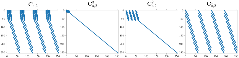
Figure 16: Sparsity patterns of two-dimensional synthesis convolution matrices. Upper indices indicate individual scale matrices. The transformation matrix on the left is the matrix-product of all three scale-matrices.

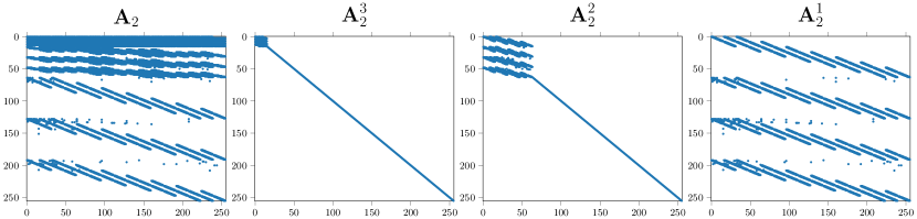
Figure 17: Sparsity patterns of two-dimensional analysis fwt-matrices. Upper indices indicate individual scale matrices. The transformation matrix on the left is the matrix-product of all three scale-matrices.

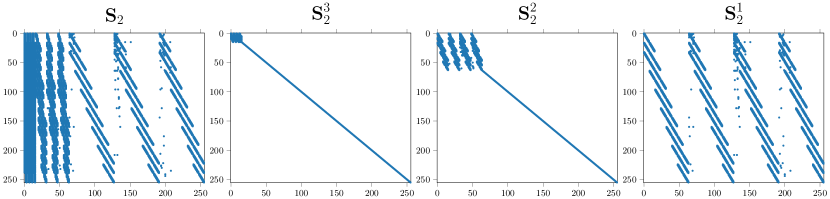
Figure 18: Sparsity patterns of two-dimensional synthesis or ifwt matrices. Upper indices indicate individual scale matrices. The transformation matrix on the left is the matrix-product of all three scale-matrices.

Figures 3, 16, 17 and 18. Illustrate the differences between two dimensional convolution and orthogonal fast wavelet transformation matrices. In comparison to the convolution matrices in Figures 3 and 16, the orthogonalization procedure has created additional entries in the two dimensional analysis and synthesis matrices on display in Figures 17 and 18.

9.6 Hyperparameters

Unless explicitly stated otherwise, we train with a batch size of 512 and a learning rate of 0.001 using Adam (Kingma and Ba,, 2015) for ten epochs. For the 5 repetitions we report, the seed values are always 0,1,2,3,4.

9.7 Detection of images from an unknown generator

To exemplarily study the detection of images from an unknown gan, we remove the SN-DCGAN generated images from our lsun training and validation sets. 10,000 SN-DCGAN images now appear exclusively in the test set, where they never influence the learning process. The training hyperparameters are identical to those discussed in section 5.2. We rebalance the data to contain equally many real and GAN-generated images. The task now is to produce a real or fake label in the presence of fake images which were not present during the optimization process. For this initial proof-of-concept investigation, we apply only the simple Haar wavelet. We find that our approach does allow detection of the SN-DCGAN samples on lsun-bedrooms, without their presence in the training set. Using the $\ln$-scaled Haar-Wavelet packages, we achieve for the unknown gan a result of $78.8\pm 1.8\%$, with a max of $81.7\%$. For the real and artificial generators present in the training set, we achieve $98.6\pm 0.1\%$, with a max of 98.6%. The accuracy improvement in comparison to Table 2 likely is due to the binary classification problem here instead of the multi-classification one before. This result indicates that the wavelet representation alone can allow a transfer to unseen generators, or other manipulations, to some extent.

9.8 lsun perturbation analysis

Table 8: Perturbation analysis of the db3 wavelet-packet- and pixel- cnn classifiers on lsun-bedrooms.

		Accuracy on lsun[%]
Method	Perturbation	$\max$	$\mu\pm\sigma$
CNN-$\ln$-db3 (ours)	center-crop	95.68	95.49$\pm$ 0.26
CNN-Pixel (ours)	center-crop	92.03	90.04$\pm$ 1.18
CNN-$\ln$-db3 (ours)	rotation	91.74	90.84$\pm$ 0.90
CNN-Pixel (ours)	rotation	92.63	91.99$\pm$ 0.97
CNN-$\ln$-db3 (ours)	jpeg	84.73	84.25 $\pm$ 00.33
CNN-Pixel (ours)	jpeg	89.95	89.25 $\pm$ 00.48

We study the effect of image cropping, rotation, and jpeg compression on our classifiers in table 8. We re-trained both classifiers on the perturbed data as described in section 5.2. The center crop perturbation randomly extracts images centers while preserving at least 80% of the original width or height. Both the pixel and packet approaches are affected by center cropping yet can classify more than 90% of all images correctly. In this case, the log-scaled db3-wavelet packets can outperform the pixel-space representation on average. Rotation and jpeg compression change the picture. The rotation perturbation randomly rotates all images by up to $15^{\circ}$ degrees. The jpeg perturbation randomly compresses images with a compression factor drawn from $U(70,90)$, without subsampling. The wavelet-packet representation is less robust to rotation than its pixel counterpart. For jpeg-compression, the effect is more pronounced. Looking at Figure 6 suggests that our classifiers rely on high-frequency information. Since jpeg-compression removes this part of the spectrum, perhaps explaining the larger drop in mean accuracy.

[width=.45]./figures/ffhq_hard/absolute_coeff_comparison_stylegan [width=.45]./figures/ffhq_hard/absolute_coeff_comparison_stylegan2 [width=.45]./figures/ffhq_hard/absolute_coeff_comparison_stylegan3

Figure 19: Mean and standard deviation plots for the three styleGAN variants on ffhq.

9.9 Results on the full ffpp with and without image corruption

Table 9: Classification accuracies for the complete ffpp-data set. Results for no compression (C0), high quality compression (C23) as well as aggressive compression (C40) are tabulated. For comparison, we additionally cite the results presented in Rossler et al., (2019). We were able to find the parameter count for XceptionNet in Chollet, (2017) and added it to the table. XceptionNet was pretrained in Image-Net and is therefore not directly comparable to the rest of the table.

		Accuracy on ffpp C0 [%]
Method	parameters	max	$\mu\pm\sigma$
CNN-pixel (ours)	57k	97.24	$94.87\pm 1.47$
CNN-db4 (ours)	109k	96.07	$95.75\pm 0.23$
CNN-sym4 (ours)	109k	97.05	$96.45\pm 0.35$
Steg. Feat. + SVM (Fridrich and Kodovsky,)	-	97.63	-
Cozzolino et al.,	-	98.57	-
Bayar and Stamm,	-	98.74	-
Rahmouni et al.,	-	97.03	-
MesoNet (Afchar et al.,)	-	95.23	-
XceptionNet (Chollet,)	22,856k	99.26	-
		Accuracy on ffpp C23 [%]
CNN-pixel (ours)	57k	80.41	$77.97\pm 1.74$
CNN-db4 (ours)	109k	85.41	$84.49\pm 0.83$
CNN-sym4 (ours)	109k	84.48	$83.03\pm 1.16$
Steg. Feat. + SVM (Fridrich and Kodovsky,)	-	70.97	-
Cozzolino et al.,	-	78.45	-
Bayar and Stamm,	-	82.87	-
Rahmouni et al.,	-	79.08	-
MesoNet (Afchar et al.,)	-	83.10	-
XceptionNet (Chollet,)	22,856k	95.73	-
		Accuracy on ffpp C40 [%]
CNN-pixel (ours)	57k	75.54	$74.11\pm 1.87$
CNN-db4 (ours)	109k	71.91	$71.91\pm 1.03$
CNN-sym4 (ours)	109k	72.92	$69.91\pm 2.24$
Steg. Feat. + SVM (Fridrich and Kodovsky,)	-	55.98	-
Cozzolino et al.,	-	58.69	-
Bayar and Stamm,	-	66.84	-
Rahmouni et al.,	-	61.18	-
MesoNet (Afchar et al.,)	-	70.47	-
XceptionNet (Chollet,)	22,856k	81.00	-

We train our networks as previously discussed in sections 5.2 and 5.4. Table 9 lists results for a pixel-cnn as well as wavelet-packet-architectures using db4 and sym4-wavelets. In comparison to various benchmark methods our networks perform competitively. Figures 21 and  21 tell us that classical face modification methods produce fewer artifacts in the wavelet-domain. This observation probably explains the drop in performance for the network processing the uncompressed features. We note competitive performance in the high-quality (C23) case.

[width=0.48]./figures/ffpp/absolute_coeff_comparison_db4_mean_all [width=0.48]./figures/ffpp/absolute_coeff_comparison_sym4_mean_all [width=0.48]./figures/ffpp/absolute_coeff_comparison_db4_grouped [width=0.48]./figures/ffpp/absolute_coeff_comparison_sym4_grouped

Figure 20: Mean $\ln$-wavelet packet plots for all elements of the FaceForensics++ training set for the db4-wavelet (left) and the sym4-wavelet(right). A full list of the order of packets can be found in Figure 23. Generally the frequencies increase from left to right. We observe a difference between the means of machine learning based fakes (Deepfakes (Deepfake-Faceswap-Contributors,, 2018) and NeuralTextures (Thies et al.,, 2019)) and the other methods, especially in the higher frequencies i.e. on the right hand side (best observed when zoomed into the plot).

Figure 21: Wavelet packet mean and standard deviation using db4-wavelets (left) and sym4-wavelets (right) for the original data, machine learning-based methods, and classic computer-vision methods. Again, we see a difference in the mean of machine learning-based models and the other sources as well as the original data.

Table 10: Confusion matrix for the $\ln$-db4-cnn on the extended ffhq problem.

	Predicted label
True label	ffhq	StyleGAN	StyleGAN2	StyleGAN3
ffhq	4626	0	14	360
StyleGAN	4	4991	0	5
StyleGAN2	13	0	4913	74
StyleGAN3	237	0	80	4683

9.10 Packet labels

[width=.48]figures/concept/packet_labels

Figure 22: Labels for the transforms of level 3 we showed previously in the frequency order. For an excellent introduction to the theory behind the frequency order see Jensen and la Cour-Harbo, (2001).

1. aaa

2. aah

3. aav

4. aad

5. aha

6. ahh

7. ahv

8. ahd

9. ava

10. avh

11. avv

12. avd

13. ada

14. adh

15. adv

16. add

17. haa

18. hah

19. hav

20. had

21. hha

22. hhh

23. hhv

24. hhd

25. hva

26. hvh

27. hvv

28. hvd

29. hda

30. hdh

31. hdv

32. hdd

33. vaa

34. vah

35. vav

36. vad

37. vha

38. vhh

39. vhv

40. vhd

41. vva

42. vvh

43. vvv

44. vvd

45. vda

46. vdh

47. vdv

48. vdd

49. daa

50. dah

51. dav

52. dad

53. dha

54. dhh

55. dhv

56. dhd

57. dva

58. dvh

59. dvv

60. dvd

61. dda

62. ddh

63. ddv

64. ddd

Figure 23: Order of wavelet packet coefficients as used in the mean absolute coefficient plots.

Figure 23 displays the 1d ordering and Figure 22 the 2d ordering of the 64 image-patches of the level 3 wavelet packet coefficients. Each reappear many times in the paper.

9.11 Reproducibility Statement

To ensure the reproducibility of this research project, we release our wavelet toolbox and the source code for our experiments in the supplementary material. The wavelet toolbox ships multiple unit tests to ensure correctness. Our code is carefully documented to make it as accessible as possible. We have consistently seeded the Mersenne twister used by PyTorch to initialize our neural networks with 0, 1, 2, 3, 4. Since the seed is always set, rerunning our code always produces the same results. Outliers can make it hard to reproduce results if the seed is unknown. To ensure we do not share outliers without context, we report mean and standard deviations of five runs for all neural network experiments.

References

- Afchar et al., (2018) Afchar, D., Nozick, V., Yamagishi, J., and Echizen, I. (2018). Mesonet: a compact facial video forgery detection network. In 2018 IEEE international workshop on information forensics and security (WIFS), pages 1–7. IEEE.
- Antipov et al., (2017) Antipov, G., Baccouche, M., and Dugelay, J.-L. (2017). Face aging with conditional generative adversarial networks. In 2017 IEEE international conference on image processing (ICIP), pages 2089–2093. IEEE.
- Applebaum, (2020) Applebaum, A. (2020). Twilight of Democracy: The Seductive Lure of Authoritarianism. Doubleday.
- Bayar and Stamm, (2016) Bayar, B. and Stamm, M. C. (2016). A deep learning approach to universal image manipulation detection using a new convolutional layer. In Proceedings of the 4th ACM workshop on information hiding and multimedia security, pages 5–10.
- Bellemare et al., (2017) Bellemare, M. G., Danihelka, I., Dabney, W., Mohamed, S., Lakshminarayanan, B., Hoyer, S., and Munos, R. (2017). The cramer distance as a solution to biased wasserstein gradients. CoRR, abs/1705.10743.
- Binkowski et al., (2018) Binkowski, M., Sutherland, D. J., Arbel, M., and Gretton, A. (2018). Demystifying MMD gans. In 6th International Conference on Learning Representations, ICLR 2018, Vancouver, BC, Canada, April 30 - May 3, 2018, Conference Track Proceedings. OpenReview.net.
- Brock et al., (2019) Brock, A., Donahue, J., and Simonyan, K. (2019). Large scale GAN training for high fidelity natural image synthesis. In 7th International Conference on Learning Representations, ICLR 2019, New Orleans, LA, USA, May 6-9, 2019. OpenReview.net.
- Bruna and Mallat, (2013) Bruna, J. and Mallat, S. (2013). Invariant scattering convolution networks. IEEE Transactions on Pattern Analysis and Machine Intelligence, 35:1872–1886.
- Chen et al., (2015) Chen, L.-l., Zhao, Y., Zhang, J., and Zou, J.-z. (2015). Automatic detection of alertness/drowsiness from physiological signals using wavelet-based nonlinear features and machine learning. Expert Systems with Applications, 42(21):7344–7355.
- Chollet, (2017) Chollet, F. (2017). Xception: Deep learning with depthwise separable convolutions. 2017 IEEE Conference on Computer Vision and Pattern Recognition (CVPR), pages 1800–1807.
- Cotter, (2020) Cotter, F. (2020). Uses of Complex Wavelets in Deep Convolutional Neural Networks. PhD thesis, University of Cambridge.
- Cozzolino et al., (2017) Cozzolino, D., Poggi, G., and Verdoliva, L. (2017). Recasting residual-based local descriptors as convolutional neural networks: an application to image forgery detection. In Proceedings of the 5th ACM Workshop on Information Hiding and Multimedia Security, pages 159–164.
- Daubechies, (1992) Daubechies, I. (1992). Ten Lectures on Wavelets. SIAM.
- Deepfake-Faceswap-Contributors, (2018) Deepfake-Faceswap-Contributors (2018). Deepfake-faceswap. https://github.com/deepfakes/faceswap. Accessed: 2022-2-07.
- Dhariwal and Nichol, (2021) Dhariwal, P. and Nichol, A. (2021). Diffusion models beat gans on image synthesis. Advances in Neural Information Processing Systems, 34.
- Durall et al., (2020) Durall, R., Keuper, M., and Keuper, J. (2020). Watch your up-convolution: Cnn based generative deep neural networks are failing to reproduce spectral distributions. In Proceedings of the IEEE/CVF Conference on Computer Vision and Pattern Recognition, pages 7890–7899.
- Durall et al., (2019) Durall, R., Keuper, M., Pfreundt, F.-J., and Keuper, J. (2019). Unmasking deepfakes with simple features. arXiv preprint arXiv:1911.00686.
- Dzanic et al., (2020) Dzanic, T., Shah, K., and Witherden, F. D. (2020). Fourier spectrum discrepancies in deep network generated images. In Larochelle, H., Ranzato, M., Hadsell, R., Balcan, M., and Lin, H., editors, Advances in Neural Information Processing Systems 33: Annual Conference on Neural Information Processing Systems 2020, NeurIPS 2020, December 6-12, 2020, virtual.
- Frank et al., (2020) Frank, J., Eisenhofer, T., Schönherr, L., Fischer, A., Kolossa, D., and Holz, T. (2020). Leveraging frequency analysis for deep fake image recognition. In Proceedings of the 37th International Conference on Machine Learning, ICML 2020, 13-18 July 2020, Virtual Event, volume 119 of Proceedings of Machine Learning Research, pages 3247–3258. PMLR.
- Fridrich and Kodovsky, (2012) Fridrich, J. and Kodovsky, J. (2012). Rich models for steganalysis of digital images. IEEE Transactions on information Forensics and Security, 7(3):868–882.
- Gal et al., (2021) Gal, R., Hochberg, D. C., Bermano, A., and Cohen-Or, D. (2021). Swagan: A style-based wavelet-driven generative model. ACM Transactions on Graphics (TOG), 40(4):1–11.
- Gatys et al., (2016) Gatys, L. A., Ecker, A. S., and Bethge, M. (2016). Image style transfer using convolutional neural networks. In 2016 IEEE Conference on Computer Vision and Pattern Recognition, CVPR 2016, Las Vegas, NV, USA, June 27-30, 2016, pages 2414–2423. IEEE Computer Society.
- Giudice et al., (2021) Giudice, O., Guarnera, L., and Battiato, S. (2021). Fighting Deepfakes by Detecting GAN DCT Anomalies. Journal of Imaging, 7(8):128.
- Goodfellow et al., (2014) Goodfellow, I. J., Pouget-Abadie, J., Mirza, M., Xu, B., Warde-Farley, D., Ozair, S., Courville, A. C., and Bengio, Y. (2014). Generative adversarial nets. In NIPS.
- Guarnera et al., (2020) Guarnera, L., Giudice, O., and Battiato, S. (2020). Fighting deepfake by exposing the convolutional traces on images. IEEE Access.
- Gui et al., (2022) Gui, J., Sun, Z., Wen, Y., Tao, D., and Ye, J. (2022). A Review on Generative Adversarial Networks: Algorithms, Theory, and Applications. IEEE Transactions on Knowledge and Data Engineering, 14(8):1–1.
- Ha et al., (2021) Ha, W., Singh, C., Lanusse, F., Upadhyayula, S., and Yu, B. (2021). Adaptive wavelet distillation from neural networks through interpretations. Advances in Neural Information Processing Systems, 34.
- He et al., (2021) He, Y., Yu, N., Keuper, M., and Fritz, M. (2021). Beyond the spectrum: Detecting deepfakes via re-synthesis. In Zhou, Z., editor, Proceedings of the Thirtieth International Joint Conference on Artificial Intelligence, IJCAI 2021, Virtual Event / Montreal, Canada, 19-27 August 2021, pages 2534–2541. ijcai.org.
- Ho et al., (2020) Ho, J., Jain, A., and Abbeel, P. (2020). Denoising Diffusion Probabilistic Models. In Larochelle, H., Ranzato, M., Hadsell, R., Balcan, M. F., and Lin, H., editors, Advances in Neural Information Processing Systems, volume 33, pages 6840–6851. Curran Associates, Inc.
- Jensen and la Cour-Harbo, (2001) Jensen, A. and la Cour-Harbo, A. (2001). Ripples in mathematics: the discrete wavelet transform. Springer Science & Business Media.
- Karras et al., (2018) Karras, T., Aila, T., Laine, S., and Lehtinen, J. (2018). Progressive growing of gans for improved quality, stability, and variation. In 6th International Conference on Learning Representations, ICLR 2018, Vancouver, BC, Canada, April 30 - May 3, 2018, Conference Track Proceedings.
- Karras et al., (2021) Karras, T., Aittala, M., Laine, S., Härkönen, E., Hellsten, J., Lehtinen, J., and Aila, T. (2021). Alias-free generative adversarial networks. CoRR, abs/2106.12423.
- Karras et al., (2019) Karras, T., Laine, S., and Aila, T. (2019). A style-based generator architecture for generative adversarial networks.
- Karras et al., (2020) Karras, T., Laine, S., Aittala, M., Hellsten, J., Lehtinen, J., and Aila, T. (2020). Analyzing and improving the image quality of stylegan. In Proceedings of the IEEE/CVF Conference on Computer Vision and Pattern Recognition, pages 8110–8119.
- Kingma and Ba, (2015) Kingma, D. P. and Ba, J. (2015). Adam: A method for stochastic optimization. In Bengio, Y. and LeCun, Y., editors, 3rd International Conference on Learning Representations, ICLR 2015, San Diego, CA, USA, May 7-9, 2015, Conference Track Proceedings.
- Kowalski, (2016) Kowalski, M. (2016). Faceswap-contributors. https://github.com/MarekKowalski/FaceSwap/. Accessed: 2022-2-07.
- Liu et al., (2015) Liu, Z., Luo, P., Wang, X., and Tang, X. (2015). Deep learning face attributes in the wild. In Proceedings of International Conference on Computer Vision (ICCV).
- Mallat, (1989) Mallat, S. (1989). A theory for multiresolution signal decomposition: the wavelet representation. IEEE transactions on pattern analysis and machine intelligence, 11(7):674–693.
- Mallat, (2009) Mallat, S. (2009). A Wavelet Tour of Signal Processing, The Sparse Way. Academic Press, Elsevier.
- Mallat, (2012) Mallat, S. (2012). Group invariant scattering. Communications on Pure and Applied Mathematics, 65(10):1331–1398.
- Marra et al., (2019) Marra, F., Gragnaniello, D., Verdoliva, L., and Poggi, G. (2019). Do gans leave artificial fingerprints? In 2019 IEEE Conference on Multimedia Information Processing and Retrieval (MIPR), pages 506–511. IEEE.
- Miyato et al., (2018) Miyato, T., Kataoka, T., Koyama, M., and Yoshida, Y. (2018). Spectral normalization for generative adversarial networks. In 6th International Conference on Learning Representations, ICLR 2018, Vancouver, BC, Canada, April 30 - May 3, 2018, Conference Track Proceedings.
- Oyallon and Mallat, (2015) Oyallon, E. and Mallat, S. (2015). Deep roto-translation scattering for object classification. In Proceedings of the IEEE Conference on Computer Vision and Pattern Recognition, pages 2865–2873.
- Parkin, (2012) Parkin, S. (2012). The rise of the deepfake and the threat to democracy. https://www.theguardian.com/technology/ng-interactive/2019/jun/22/the-rise-of-the-deepfake-and-the-threat-to-democracy. Accessed: 2021-05-10.
- Paszke et al., (2017) Paszke, A., Gross, S., Chintala, S., Chanan, G., Yang, E., DeVito, Z., Lin, Z., Desmaison, A., Antiga, L., and Lerer, A. (2017). Automatic differentiation in pytorch. NIPS 2017 Autodiff-Workshop.
- Paszke et al., (2019) Paszke, A., Gross, S., Massa, F., Lerer, A., Bradbury, J., Chanan, G., Killeen, T., Lin, Z., Gimelshein, N., Antiga, L., Desmaison, A., Köpf, A., Yang, E., DeVito, Z., Raison, M., Tejani, A., Chilamkurthy, S., Steiner, B., Fang, L., Bai, J., and Chintala, S. (2019). Pytorch: An imperative style, high-performance deep learning library. In Advances in Neural Information Processing Systems 32: Annual Conference on Neural Information Processing Systems 2019, NeurIPS 2019.
- Rahmouni et al., (2017) Rahmouni, N., Nozick, V., Yamagishi, J., and Echizen, I. (2017). Distinguishing computer graphics from natural images using convolution neural networks. In 2017 IEEE Workshop on Information Forensics and Security (WIFS). IEEE.
- Rossler et al., (2019) Rossler, A., Cozzolino, D., Verdoliva, L., Riess, C., Thies, J., and Nießner, M. (2019). Faceforensics++: Learning to detect manipulated facial images. In Proceedings of the IEEE/CVF International Conference on Computer Vision, pages 1–11.
- Schwarz et al., (2021) Schwarz, K., Liao, Y., and Geiger, A. (2021). On the frequency bias of generative models. Advances in Neural Information Processing Systems, 34.
- Simonyan et al., (2014) Simonyan, K., Vedaldi, A., and Zisserman, A. (2014). Deep inside convolutional networks: Visualising image classification models and saliency maps. In Bengio, Y. and LeCun, Y., editors, 2nd International Conference on Learning Representations, ICLR 2014.
- Sirovich and Kirby, (1987) Sirovich, L. and Kirby, M. (1987). Low-dimensional procedure for the characterization of human faces. Josa a, 4(3):519–524.
- Song et al., (2021) Song, Y., Sohl-Dickstein, J., Kingma, D. P., Kumar, A., Ermon, S., and Poole, B. (2021). Score-based generative modeling through stochastic differential equations. In International Conference on Learning Representations.
- Strang and Nguyen, (1996) Strang, G. and Nguyen, T. (1996). Wavelets and filter banks. SIAM.
- Tang et al., (2021) Tang, G., Sun, L., Mao, X., Guo, S., Zhang, H., and Wang, X. (2021). Detection of GAN-Synthesized Image Based on Discrete Wavelet Transform. Security and Communication Networks, 2021:1–10.
- Taubman and Marcellin, (2002) Taubman, D. S. and Marcellin, M. W. (2002). Jpeg2000: Standard for interactive imaging. Proceedings of the IEEE, 90(8):1336–1357.
- Thies et al., (2019) Thies, J., Zollhöfer, M., and Nießner, M. (2019). Deferred neural rendering: Image synthesis using neural textures. ACM Transactions on Graphics (TOG), 38(4):1–12.
- Thies et al., (2016) Thies, J., Zollhofer, M., Stamminger, M., Theobalt, C., and Nießner, M. (2016). Face2face: Real-time face capture and reenactment of rgb videos. In Proceedings of the IEEE conference on computer vision and pattern recognition, pages 2387–2395.
- Van den Berg, (2004) Van den Berg, J. (2004). Wavelets in Physics. Cambridge University Press.
- Vyas et al., (2018) Vyas, A., Yu, S., and Paik, J. (2018). Multiscale transforms with application to image processing. Springer.
- Wang and Deng, (2021) Wang, C. and Deng, W. (2021). Representative forgery mining for fake face detection. In Proceedings of the IEEE/CVF Conference on Computer Vision and Pattern Recognition, pages 14923–14932.
- (61) Wang, R., Juefei-Xu, F., Ma, L., Xie, X., Huang, Y., Wang, J., and Liu, Y. (2020a). FakeSpotter: A Simple yet Robust Baseline for Spotting AI-Synthesized Fake Faces. In Proceedings of the Twenty-Ninth International Joint Conference on Artificial Intelligence, volume 2021-Janua.
- (62) Wang, S.-Y., Wang, O., Zhang, R., Owens, A., and Efros, A. A. (2020b). Cnn-generated images are surprisingly easy to spot… for now. In Proceedings of the IEEE/CVF Conference on Computer Vision and Pattern Recognition, pages 8695–8704.
- (63) Wang, Y. G., Li, M., Ma, Z., Montufar, G., Zhuang, X., and Fan, Y. (2020c). Haar graph pooling. In International Conference on Machine Learning, pages 9952–9962. PMLR.
- Williams and Li, (2018) Williams, T. and Li, R. (2018). Wavelet pooling for convolutional neural networks. In International Conference on Learning Representations.
- Wolter and Garcke, (2021) Wolter, M. and Garcke, J. (2021). Adaptive wavelet pooling for convolutional neural networks. In International Conference on Artificial Intelligence and Statistics, pages 1936–1944. PMLR.
- Younus and Hasan, (2020) Younus, M. A. and Hasan, T. M. (2020). Effective and fast deepfake detection method based on haar wavelet transform. In 2020 International Conference on Computer Science and Software Engineering (CSASE), pages 186–190. IEEE.
- Yu et al., (2015) Yu, F., Zhang, Y., Song, S., Seff, A., and Xiao, J. (2015). Lsun: Construction of a large-scale image dataset using deep learning with humans in the loop. arXiv preprint arXiv:1506.03365.
- Yu et al., (2019) Yu, N., Davis, L. S., and Fritz, M. (2019). Attributing fake images to gans: Learning and analyzing gan fingerprints. In Proceedings of the IEEE/CVF International Conference on Computer Vision, pages 7556–7566.
- Zhang et al., (1995) Zhang, J., Walter, G. G., Miao, Y., and Lee, W. N. W. (1995). Wavelet neural networks for function learning. IEEE transactions on Signal Processing, 43(6):1485–1497.
- Zhang, (2022) Zhang, T. (2022). Deepfake generation and detection, a survey. Multimedia Tools and Applications.
- Zhang et al., (2019) Zhang, X., Karaman, S., and Chang, S.-F. (2019). Detecting and simulating artifacts in gan fake images. In 2019 IEEE International Workshop on Information Forensics and Security (WIFS), pages 1–6. IEEE.
- (72) Zhao, H., Zhou, W., Chen, D., Wei, T., Zhang, W., and Yu, N. (2021a). Multi-attentional deepfake detection. In Proceedings of the IEEE/CVF Conference on Computer Vision and Pattern Recognition, pages 2185–2194.
- (73) Zhao, T., Xu, X., Xu, M., Ding, H., Xiong, Y., and Xia, W. (2021b). Learning self-consistency for deepfake detection. In Proceedings of the IEEE/CVF International Conference on Computer Vision, pages 15023–15033.