Large Scale Private Learning via Low-rank Reparametrization

Abstract

We propose a reparametrization scheme to address the challenges of applying differentially private SGD on large neural networks, which are 1) the huge memory cost of storing individual gradients, 2) the added noise suffering notorious dimensional dependence. Specifically, we reparametrize each weight matrix with two gradient-carrier matrices of small dimension and a residual weight matrix. We argue that such reparametrization keeps the forward/backward process unchanged while enabling us to compute the projected gradient without computing the gradient itself. To learn with differential privacy, we design reparametrized gradient perturbation (RGP) that perturbs the gradients on gradient-carrier matrices and reconstructs an update for the original weight from the noisy gradients. Importantly, we use historical updates to find the gradient-carrier matrices, whose optimality is rigorously justified under linear regression and empirically verified with deep learning tasks. RGP significantly reduces the memory cost and improves the utility. For example, we are the first able to apply differential privacy on the BERT model and achieve an average accuracy of $83.9\%$ on four downstream tasks with $\epsilon=8$, which is within $5\%$ loss compared to the non-private baseline but enjoys much lower privacy leakage risk.

[name=Theorem,numberwithin=section]thm [name=Proposition,numberwithin=section]pro

1 Introduction

A recent line of works (Shokri et al., 2017; Carlini et al., 2019, 2020) have exposed the potential privacy risks of trained models, e.g., data extraction from language model. Theoretically, learning with differential privacy (Dwork et al., 2006) is guaranteed to prevent such information leakage because differential privacy imposes an upper bound on the influence of any individual sample. Empirically, differential privacy also makes learning more resistant to attacks (Rahman et al., 2018; Bernau et al., 2019; Zhu et al., 2019; Carlini et al., 2019; Ma et al., 2019; Lecuyer et al., 2019).

To learn with differential privacy, many algorithms have been proposed under different settings over the past decade, e.g., Chaudhuri & Monteleoni (2009); Song et al. (2013); Agarwal et al. (2018); Wang & Gu (2019); Wang et al. (2019a); Yu et al. (2020); Phan et al. (2020); Vietri et al. (2020), to name a few. Among them, gradient perturbation is a popular choice because of its simplicity and wide applicability (Abadi et al., 2016). In terms of simplicity, gradient perturbation only makes two simple modifications to the standard learning process. It first clips the gradients of individual samples, referred to as individual gradients, to bound the sensitivity and then perturbs the aggregated gradient with random noise. In terms of wide applicability, it does not assume the objective to be convex and hence applies to deep neural networks.

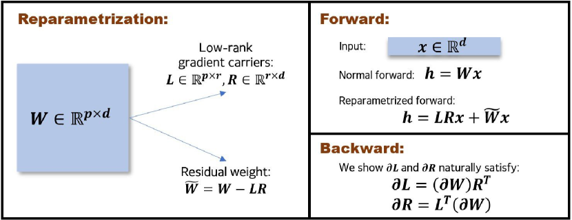
Figure 1: The proposed reparametrization scheme. The residual weight makes the reparametrized output the same as the normal output and $\partial{\bm{L}}$, $\partial{\bm{R}}$ naturally connected with the normal gradient.

Despite its advantages, there are two challenges when applying gradient perturbation to cutting-edge deep models. First, one needs to compute and store individual gradients. Recent works (Dangel et al., 2019; Opacus, 2020) have developed toolkits to compute individual gradients for a mini-batch of data through a single forward/backward pass, but storing individual gradients consumes a huge amount of memory as each individual gradient requires the same amount of memory as the model itself. Second, both theoretical and empirical utilities of gradient perturbation suffer from bad dependence on the model size (Bassily et al., 2014; Papernot et al., 2020; Tramèr & Boneh, 2021) because the intensity of the added noise scales proportionally with the model size.

To tackle these challenges, we reparameterize each weight matrix ${\bm{W}}$ of a deep neural network with a pair of low-rank gradient carriers $\{{\bm{L}},{\bm{R}}\}$ and a residual weight $\tilde{{\bm{W}}}$, as illustrated in Figure 1. With this reparametrization, the forward signal and the backward signal propagate the same as before. We show that the gradients on ${\bm{L}}$ and ${\bm{R}}$ are naturally connected with the gradient on ${\bm{W}}$. Especially if the gradient carriers consist of orthonormal vectors, we can construct a projection of the gradient of ${\bm{W}}$ from the gradients of ${\bm{L}}$ and ${\bm{R}}$ that are of low dimension. In other words, we can compute the projection of the gradient without computing the gradient itself. This property could save a huge amount of memory in DP-SGD where a large batch of individual gradients are computed and stored. We note that this could be also useful in other problems involving statistics of individual gradients, e.g. computing the gradient variance (Zhao & Zhang, 2015; Balles et al., 2016; Mahsereci & Hennig, 2017; Balles & Hennig, 2018), which is out of our scope.

Based on the above framework, we propose reparametrized gradient perturbation (RGP) for differentially private learning. Specifically, after the backward process, RGP clips and perturbs the gradients of ${\bm{L}}$ and ${\bm{R}}$, which gives a certain level of privacy guarantee. Then RGP uses the noisy gradients to construct an update for the original weight. We note that because the gradient-carrier matrices are of much smaller dimension than the original weight matrix, the total intensity of the added noises is significantly smaller, which helps us break the notorious dimensional dependence of the utility of differentially private learning.

The key of the reparameterization scheme is how well the gradient projection approximates the original gradient. We argue that the approximation is good if 1) the original gradient of ${\bm{W}}$ itself is indeed low-rank and 2) its principal subspace aligns with ${\bm{L}}$ and ${\bm{R}}$. The first condition is empirically verified by showing the gradient of each layer is of low stable rank when training deep neural networks, which has also been exploited for gradient compression in distributed optimization (Vogels et al., 2019). The second condition is guaranteed if ${\bm{L}}$ and ${\bm{R}}$ consists of the principal singular vectors of the original gradient, which, however, violates the differential privacy. Instead, in RGP, we approximately compute a few of principal vectors of the historical updates that are already published and free to use because of the post-processing property of differential privacy, and use them as gradient carriers. We theoretically prove that the optimality of using the historical update substitution for linear regression and empirically verify its efficacy for deep neural networks.

With RGP, we can easily train large models with differential privacy and achieve good utility on both the vision and language modeling tasks. For example, we use RGP to train the BERT model (Devlin et al., 2018) on downstream language understanding tasks. We establish rigorous differential privacy guarantee for such large model with a modest drop in accuracy. With a privacy budget $\epsilon=8$, we achieve an average accuracy $83.9\%$ on downstream tasks, which is within $5\%$ loss compared to the non-private baseline. We also use membership inference attack (Shokri et al., 2017; Sablayrolles et al., 2019) to evaluate the empirical privacy risks and demonstrate that the models trained with RGP are significantly more robust to membership inference attack than the non-private ones. Overall, our contribution can be summarized as follows.

1. We propose reparametrized gradient perturbation (RGP) that reduces the memory cost and improves the utility when applying DP on large models.

2. We give a detailed analysis on the property of RGP. We propose using the historical update to find the principal subspace and give theoretical arguments.

3. Empirically we are able to efficiently train BERT with differential privacy on downstream tasks, and achieve both good accuracy and privacy protection.

1.1 Notations

We introduce some basic notations. Vectors and matrices are denoted with bold lowercase letters, e.g., ${\bm{v}}$, and bold capital letters, e.g., ${\bm{M}}$, respectively. Sets are denoted with double-struck capital letters, e.g., ${\mathbb{S}}$. We use $[n]$ to denote the set of positive numbers $\{1,...,n\}$. Some preliminaries on differential privacy are presented in Appendix A.

2 A Reparametrization Scheme

In this section, we introduce a reparametrization scheme for the neural network weight matrices so that computing and storing individual gradients are affordable for large models. Specifically, during each forward/backward process, for a layer with weight matrix ${\bm{W}}\in{\mathbb{R}}^{p\times d}$, we reparametrize it as follows (see Figure 1 for an illustration),

$${\bm{W}}\rightarrow{\bm{L}}{\bm{R}}+\tilde{{\bm{W}}}.{stop\_gradient()},$$ (1)

where ${\bm{L}}\in{\mathbb{R}}^{p\times r},{\bm{R}}\in{\mathbb{R}}^{r\times d}$ are two low-rank gradient carriers with $r\ll p\text{ or }d$, $\tilde{{\bm{W}}}={\bm{W}}-{\bm{L}}{\bm{R}}$ represents the residual weight and $.{stop\_gradient()}$ means that we do not collect the gradient on $\tilde{{\bm{W}}}$. Hence, such reparametrization does not change the forward signal and the backward signal, but only changes the gradient computation. Now we obtain the gradients on ${\bm{L}}$ and ${\bm{R}}$. We then unveil the connection between the gradient on ${\bm{W}}$ and the gradients on ${\bm{L}}$ and ${\bm{R}}$.

Theorem 2.1.

For a layer with weight matrix ${\bm{W}}$, suppose that $\partial{\bm{W}}$ is the gradient computed by back-propagation with a mini-batch data ${\mathbb{D}}$. Given two matrices ${\bm{L}},{\bm{R}}$, we reparametrize ${\bm{W}}$ as in Eq (1) and compute the gradients $\partial{\bm{L}}$ and $\partial{\bm{R}}$ by running the forward and backward process with the same mini-batch ${\mathbb{D}}$, then

$$\partial{\bm{L}}=(\partial{\bm{W}}){\bm{R}}^{T},\;\;\partial{\bm{R}}={\bm{L}}^{T}(\partial{\bm{W}}).$$ (2)

Based on the above understanding, we can construct an update for ${\bm{W}}$ by using $\partial{\bm{L}}$ and $\partial{\bm{R}}$.

Corollary 2.1.1.

If the columns of ${\bm{L}}$ and the rows of ${\bm{R}}$ are orthonormal, respectively, and we use

$$(\partial{\bm{L}}){\bm{R}}+{\bm{L}}(\partial{\bm{R}})-{\bm{L}}{\bm{L}}^{T}(\partial{\bm{L}}){\bm{R}},$$ (3)

as the update for ${\bm{W}}$, then the update is equivalent to projecting $\partial{\bm{W}}$ into the subspace of matrices whose row/column spaces are spanned by ${\bm{L}}$ and ${\bm{R}}$.

Proof.

The proofs of Theorem 2.1 and Corollary 2.1.1 are relegated to Appendix B.1. ∎

We note that if ${\bm{L}}$ and ${\bm{R}}$ consist of orthonormal bases, Corollary 2.1.1 states that we can obtain the projection of $\partial{\bm{W}}$ without explicitly computing and storing $\partial{\bm{W}}$! The size of gradient on ${\bm{L}}$ or ${\bm{R}}$ is much smaller than the size of $\partial{\bm{W}}$ if the gradient carriers are chosen to be low-rank. Therefore, this reparametrization provides a convenient way to compute and store projected gradients of a large matrix. This is extremely beneficial for the scenarios where individual gradients $\{\partial_{i}{\bm{W}}\}_{i=1}^{m}$ are required, e.g., approximating the variance of gradients and controlling the gradient sensitivity.

It is natural to ask how to choose ${\bm{L}}$ and ${\bm{R}}$ so that the update in Corollary 2.1.1 contains the most information of $\partial{\bm{W}}$. Ideally, we can first compute the aggregated gradient $\partial{\bm{W}}$ and run singular value decomposition (SVD) $\partial{\bm{W}}={\bm{U}}{\bm{\Sigma}}{\bm{V}}^{T}$. Then we can choose the top few columns of ${\bm{U}}$ and ${\bm{V}}$ to serve as the gradient carriers. In this case, the update in Corollary 2.1.1 is equivalent to approximating $\partial{\bm{W}}$ with its top-$r$ principal components.

However, in the context of differential privacy, we can not directly decompose $\partial{\bm{W}}$ as it is private. In the sequel, we give a practical reparametrization scheme for differentially private learning, where we use the historical update to find ${\bm{L}}$ and ${\bm{R}}$ and argue the optimality under certain conditions.

One may wonder why not just replace ${\bm{W}}$ with ${\bm{L}}$ and ${\bm{R}}$ instead of doing the reparametrization. We note that the forward and the backward process remain the same as before if doing the reparametrization, and the only change is the gradient computation of ${\bm{W}}$. In contrast, if using ${\bm{L}}$ and ${\bm{R}}$ to replace the weight ${\bm{W}}$, this would not only reduce the expressive power but also hurt the optimization as the width varies dramatically across layers and the forward/backward signals cannot propagate well by common initialization strategies (Glorot & Bengio, 2010; He et al., 2016).

2.1 Reparametrization for Convolutional Layers

In the above, we have described how to reparametrize a weight matrix, which covers the usual fully-connected layer and the attention layer in language models. In this subsection, we show the reparametrization of convolutional layers. Let ${\bm{x}}\in\mathbb{R}^{d\times w^{\prime}\times h^{\prime}}$ be the input feature maps of one sample and ${\bm{h}}\in\mathbb{R}^{p\times w\times h}$ be the output feature maps. We describe how to compute the elements at one spatial position ${\bm{h}}_{:,i,j}\in\mathbb{R}^{p}$ where $i\in[0,w]$ and $j\in[0,h]$.

Let ${\bm{W}}\in\mathbb{R}^{p\times d\times k\times k}$ be the convolution kernels and ${\bm{x}}^{(i,j)}\in\mathbb{R}^{d\times k\times k}$ be the features that we need to compute ${\bm{h}}_{:,i,j}$. The output feature ${\bm{h}}_{:,i,j}$ can be computed as ${\bm{h}}_{:,i,j}=\bar{\bm{W}}{\bm{x}}^{(i,j)}$, where $\bar{\bm{W}}\in\mathbb{R}^{p\times dk^{2}}$ is obtained by flattening the channel and kernel dimensions. Hence, we can use the same way as in Eq (1) to reparametrize $\bar{\bm{W}}$:

$${\bm{h}}_{:,i,j}={\bm{L}}{\bm{R}}{\bm{x}}^{(i,j)}+(\bar{\bm{W}}-{\bm{L}}{\bm{R}}){\bm{x}}^{(i,j)}.$$ (4)

Specifically, the operation of ${\bm{R}}$ and ${\bm{L}}$ are implemented by two consequent convolutional layers with kernel sizes $r\times d\times k\times k$  and $p\times r\times 1\times 1$, respectively, where $r$ is the reparametrization rank. The residual weight is implemented by a convolutional layer of the original kernel size.

3 Private Deep Learning with Reparametrized Gradient Perturbation

The above reparametrization strategy can significantly reduce the gradient dimension, which could help us circumvent the difficulties of applying differential privacy on large machine learning models. In this section, we propose a procedure “reparametrized gradient perturbation (RGP)” to train large neural network models with differential privacy. Specifically, Section 3.1 introduces the whole procedure of RGP, Section 3.2 gives the privacy guarantee of RGP, and Section 3.3 presents the complexity analysis.

Algorithm 1 Reparametrized Gradient Perturbation (RGP)

1:  Input: NN with weight matrices $\{{\bm{W}}^{(l)}\}_{l=1}^{H}$, steps $T$, probability $q$, variance $\sigma^{2}$, clipping threshold $C$, warm-up steps $T_{\text{warm-up}}$, Algorithm 2 input $\{r,K\}$.

2:  Randomly initialize the weights and obtain $\{{\bm{W}}^{(l)}_{0}\}_{l=1}^{H}$;

3:  for $t=1$ to $T$ do

4:     Sample a minibatch $\{{\bm{x}}_{i}\}_{i\in S_{t}}$ with probability $q$;

5:     For all $l\in[H]$, compute historical updates

$$\Delta_{t}^{(l)}\leftarrow{\bm{W}}^{(l)}_{t}-{\bm{W}}^{(l)}_{0}\cdot 1_{\{t>T_{\text{warm-up}}\}};$$

and run Alg. 2 with $\{\Delta_{t}^{(l)},r,K\}$ to get ${\bm{L}}_{t}^{(l)},{\bm{R}}_{t}^{(l)}$;

6:     //Forward/backward process with reparametrization.

7:     Run reparametrized forward process with Eq (1);

8:     Run backward process and compute individual gradients $\{\partial_{i}{\bm{L}}_{t}^{(l)},\partial_{i}{\bm{R}}_{t}^{(l)}\}_{l\in[H],i\in S_{t}}$;

9:     //Bound gradient sensitivity and add noise.

10:     Clip individual gradients with $L_{2}$ norm threshold $C$;

11:     for $l=1$ to $H$ do

12:        Sum individual gradients and get $\{\partial{\bm{L}}_{t}^{(l)},\partial{\bm{R}}_{t}^{(l)}\}$;

13:        Perturbation with Gaussian noise ${\bm{z}}_{L,t}^{(l)},{\bm{z}}_{R,t}^{(l)}$ whose elements are independently from $\mathcal{N}(0,\sigma^{2}C^{2})$:

$$\tilde{\partial}{\bm{L}}_{t}^{(l)}\leftarrow\partial{\bm{L}}_{t}^{(l)}+{\bm{z}}_{L,t}^{{(l)}},\quad\tilde{\partial}{\bm{R}}_{t}^{(l)}\leftarrow\partial{\bm{R}}_{t}^{(l)}+{\bm{z}}_{R,t}^{(l)};$$

14:        Use $\tilde{\partial}{\bm{L}}_{t}^{(l)}$, $\tilde{\partial}{\bm{R}}_{t}^{(l)}$, and Eq (3) to construct $\tilde{\partial}{\bm{W}}_{t}^{(l)}$;

15:        Use off-the-shelf optimizer to get ${\bm{W}}_{t+1}^{(l)}$;

16:     end for

17:  end for

3.1 Reparametrized Gradient Perturbation Algorithm

The pseudocode of RGP is presented in Algorithm 1. The RGP proceeds for all the layers and we ignore the layer index for simplicity in the following discussion. At each update, for a layer with weight matrix ${\bm{W}}$, RGP consists of four steps: 1) generate the gradient-carrier matrices ${\bm{L}}$ and ${\bm{R}}$, 2) run the reparametrized forward/backward process and obtain the individual gradients $\{\partial_{i}{\bm{L}}\}_{i=1}^{m}$ and $\{\partial_{i}{\bm{R}}\}_{i=1}^{m}$, 3) clip and perturb the gradients, 4) reconstruct an approximated gradient on the original weight matrix.

In the RGP procedure, step 1), which is also the core challenge, is to choose “good" gradient-carrier matrices so that the reconstructed gradient can approximate the original gradient as well as possible. First, this requires for a given rank $r$, the generated gradient-carrier matrices should align with the principal components of the original gradient well. Moreover, to reconstruct the gradient in step 4), it requires the gradient carriers have orthonormal columns/rows.

For the first requirement, we use historical updates to find the gradient carriers. The historical update is not sensitive because of the post-processing property of differential privacy. In Section 4.2, we give both empirical and theoretical arguments to demonstrate that the principal subspace of the current gradient aligns with that of the historical update. In our implementation, we use a warm-up phase in which the decomposition is directly done on the weight. We approximate the principal components via the power method (Algorithm 2) instead of the time-consuming full SVD. For the second requirement, we apply the Gram-Schmidt process to orthonormalize ${\bm{L}}$ and ${\bm{R}}$.

Algorithm 2 Decomposition via Power Method.

  Input: Historical update $\Delta$, reparametrization rank $r$, number of iterations $K$.

  Output: Gradient carriers ${\bm{L}}\in\mathbb{R}^{p\times r}$, ${\bm{R}}\in\mathbb{R}^{r\times d}$.

  Initialize ${\bm{R}}$ from standard Gaussian distribution.

  for $k=1$ to $K$ do

     ${\bm{L}}\leftarrow\Delta{\bm{R}}^{T}$

     Orthonormalize the columns of ${\bm{L}}$.

     ${\bm{R}}={\bm{L}}^{T}\Delta$

  end for

  Orthonormalize the rows of ${\bm{R}}$.

  Return ${\bm{L}}$, ${\bm{R}}$

Step 2) of RGP is the reparametrization and a round of forward/backward propagations, as presented in Section 2.

Step 3) is for differential privacy guarantee. The individual gradients $\{\partial_{i}{\bm{L}},\partial_{i}{\bm{R}}\}_{i=1}^{m}$ are first clipped by a pre-defined threshold so that the sensitivity is bounded. Then, Gaussian noise is added to the aggregated gradient to establish a differential privacy bound. The energy of added noise is proportional to the dimension, i.e., the rank $r$ of the carrier matrices. Hence, in order to make the noise energy small, it encourages us to use smaller rank $r$. However, smaller rank would increase the approximation error in the step 1). In practice, we trade off these two factors to choose a proper $r$.

In step 4), we use the noisy aggregated gradients of gradient-carrier matrices to reconstruct the gradients of original weights, as depicted in Corollary 2.1.1. The reconstructed gradients can then be used by any off-the-shelf optimizer.

3.2 Privacy Analysis of RGP

The privacy bound of Algorithm 1 is given by Proposition 3.1. The derivation of Proposition 3.1 is based on the moments accountant that is proposed in Abadi et al. (2016). Moments accountant has tighter composition bound than the strong composition theorem in Dwork et al. (2014a). Moments accountant first tracks the privacy budget spent at each update. Then, it composes the spent budget of all updates and cast the final privacy cost into the classic $(\epsilon,\delta)$-differential privacy.

Proposition 3.1 (Abadi et al. (2016)).

There exist constants $c_{1}$ and $c_{2}$ so that given running steps $T$, for any $\epsilon<c_{1}q^{2}T$, Algorithm 1 is $\left(\epsilon,\delta\right)$-differentially private for any $\delta>0$ if we choose

$$\sigma\geq c_{2}\frac{q\sqrt{Tlog\left(1/\delta\right)}}{\epsilon}.$$

Proof.

The proof outline is relegated to Appendix B.2. ∎

The value of $\sigma$ in Proposition 3.1 is based on an asymptotic bound on the moments of the privacy loss random variable. In practice, one can use the numerical tools (Wang et al., 2019b; Mironov et al., 2019) to compute a tighter bound. So far we have depicted the overall picture of RGP. We next analyze the computational and memory costs of RGP and compare them with that of DP-SGD.

3.3 Complexity Analysis of RGP

For the simplicity of notations, we only give the costs of one fully connected layer at one update (including forward and backward) and assume that the weight matrix is square. The shape of weight matrix, size of minibatch, number of power iterations, and rank of reparametrization are denoted by $(d\times d)$, $m$, $K$, and $r$, respectively.

The computational overhead of RGP consists of three parts. The first part is induced by matrix multiplication of power iteration, whose complexity is $\mathcal{O}(Krd^{2})$. The second part is induced by the Gram–Schmidt process, whose complexity is $\mathcal{O}(Kr^{2}d)$. The third part of overhead is the computational cost induced by gradient carriers during the forward/backward process, which is on the order of $\mathcal{O}(mrd)$.

RGP uses much less memory than DP-SGD in the practice. Although RGP needs some extra memory to store the activation produced by the gradient carriers, it has a significant advantage over DP-SGD on the memory cost of storing individual gradients, which is one of the main challenges of learning with differential privacy. For RGP, the memory cost of individual gradients only scales linearly with model width $d$ in contrast with $d^{2}$ for DP-SGD. We summarize the computational cost of one update and the memory cost of storing individual gradients in Table 1.

Table 1: Computation and memory costs of RGP (Algorithm 1) and DP-SGD (Abadi et al., 2016), where $m$ is the size of mini-batch, $d$ is the model width, $r$ is the reparametrization rank, and $K$ is the number of power iterations.

	DP-SGD	RGP
Computational cost	$\mathcal{O}(md^{2})$	$\mathcal{O}(md^{2}+Krd^{2}+Kr^{2}d)$
Memory cost	$\mathcal{O}(md^{2})$	$\mathcal{O}(mrd)$

The low-rank nature of gradient permits us to choose a small $r$ without destroying utility (see Section 4.1). In practice, we typically choose the rank $r$ smaller than $10$. For the number of power iterations in Algorithm 2, we find that setting $K=1$ is sufficient to get good performance. Hence, in practice, we always choose small $r$ and $K$ for efficiency while not hurting the performance.

4 Two Properties of the Gradient Matrix

We show two properties of the gradients of modern deep neural networks to justify the design choices of Algorithm 1. The first property is that the gradient of each weight matrix is naturally low-rank, which motivates us to use low-rank reparameterization. The second property is that the gradient of a weight matrix along the optimization path could stay in the same subspace, which motivates us to use the historical updates to generate the gradient-carrier matrices.

4.1 Gradient Matrix Is of Low Stable Rank

Recent works have used the low-rank approximation to compress the gradients and reduce the communication cost in distributed optimization (Yurtsever et al., 2017; Wang et al., 2018b; Karimireddy et al., 2019; Vogels et al., 2019). These existing works set up a good motivation to exploit the low stable rank property of the gradients of weight matrices.

We further verify this low-rank property which may give a hint about how to set the reparameterization rank $r$ in practice. We empirically compute the stable rank ($\|\cdot\|_{F}^{2}/\|\cdot\|^{2}_{2}$) of the gradient of the weight matrices in a BERT model and a wide ResNet model. The dataset for the BERT model is SST-2 from the GLUE benchmark (Wang et al., 2018a). The dataset for the wide ResNet model is CIFAR-10 (Krizhevsky & Hinton, 2009). The experimental setup can be found in Section 5. We plot the gradient stable rank in Figure 2.

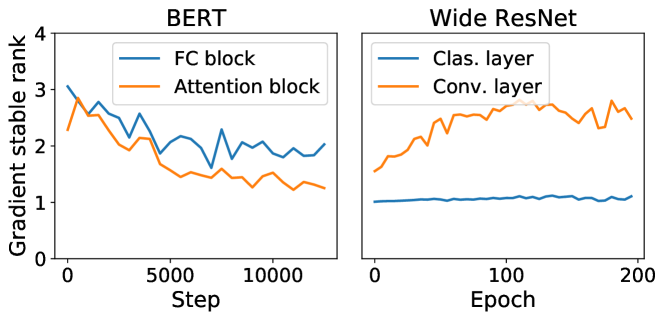
Figure 2: Gradient stable rank ($\|\cdot\|_{F}^{2}/\|\cdot\|^{2}_{2}$). For ResNet, we plot the gradient rank of the classification layer and the first residual block. For BERT, we plot the gradient rank of the first fully-connected block and the first attention block.

As shown in Figure 2, both the gradients of BERT and ResNet models are naturally of low stable rank over the training process. Hence, low-rank gradient-carrier matrices would have a small approximation error if we find the right gradient subspace. In Section 4.2, we argue that historical update is a good choice to identify the gradient subspace.

4.2 Historical Gradients Are Correlated

Suppose that ${\bm{W}}_{t}$ is a weight matrix at step $t$, and $\partial{\bm{W}}_{t}$ is the gradient with a batch of data ${\mathbb{D}}$ with a $r$-SVD $\partial{\bm{W}}_{t}={\bm{U}}_{t}\Sigma_{t}{\bm{V}}_{t}^{T}$. For another step ${t^{\prime}}$ with $t^{\prime}>t$ and the same data ${\mathbb{D}}$, we have ${\bm{W}}_{t^{\prime}},\partial{\bm{W}}_{t^{\prime}}$ and a $r$-SVD: $\partial{\bm{W}}_{t^{\prime}}={\bm{U}}_{t^{\prime}}\Sigma_{t^{\prime}}{\bm{V}}_{t^{\prime}}^{T}$. We can project $\partial{\bm{W}}_{t^{\prime}}$ onto the principal subspace of $\partial{\bm{W}}_{t}$ or $\partial{\bm{W}}_{t^{\prime}}$ and measure the projection residual

$$\|({\bm{I}}-{\bm{U}}_{t}{\bm{U}}_{t}^{T})\partial{\bm{W}}_{t^{\prime}}({\bm{I}}-{\bm{V}}_{t}{\bm{V}}_{t}^{T})\|_{F}/\|\partial{\bm{W}}_{t^{\prime}}\|_{F},$$ (5)

$$\|({\bm{I}}-{\bm{U}}_{t^{\prime}}{\bm{U}}_{t^{\prime}}^{T})\partial{\bm{W}}_{t^{\prime}}({\bm{I}}-{\bm{V}}_{t^{\prime}}{\bm{V}}_{t^{\prime}}^{T})\|_{F}/\|\partial{\bm{W}}_{t^{\prime}}\|_{F},$$ (6)

where Eq (5) is the projection residual using historical gradient, referred to as historical projection residual, and Eq (6) is the projection residual using current gradient, referred to as self projection residual. A small difference between Eq (5) and (6) indicates that the principal subspace of the current gradient aligns with that of the historical gradient.

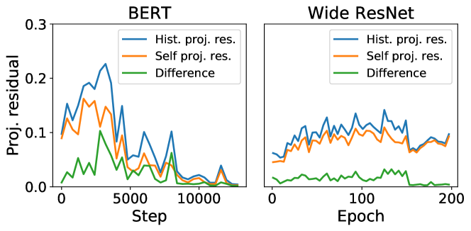
Figure 3: Projection residual with reparametrization rank $8$. We use a fixed mini-batch with $500$ samples. For ResNet, we use the input convolution layer. For BERT, we use the second matrix of the FC layer in the first encoder block. The definition of historical/self projection residual is in Eq (5) and (6).

We empirically examine the projection residual of a BERT model and a wide ResNet model. The tasks are the same as in Section 4.1. At the beginning of each epoch, we evaluate the projection residual between the current gradient and the gradient of the previous epoch. The results are plotted in Figure 3. We can see that the difference between Eq (5) and (6) is small for both models.

To understand why historical gradients are correlated, we next use a linear regression problem to rigorously show that the gradients over time could live in the same subspace. Suppose we have a set of observations $\{({\bm{x}}_{i},{\bm{y}}_{i})\}_{i=1}^{n}$, where ${\bm{x}}_{i}\in{\mathbb{R}}^{d}$ is the feature vector and ${\bm{y}}_{i}\in{\mathbb{R}}^{p}$ is the target vector for all $i\in[n]$. The least-squares problem is given by

$$\operatorname*{arg\,min}_{\bm{W}}\frac{1}{n}\sum_{i=1}^{n}\|{\bm{y}}_{i}-{\bm{W}}{\bm{x}}_{i}\|^{2}.$$ (7)

Proposition 4.1.

For the least squares problem (7), if the model is updated by gradient descent with step size $\eta$

$${\bm{W}}_{t+1}\leftarrow{\bm{W}}_{t}-\eta\cdot\partial{\bm{W}}_{t},$$ (8)

then the gradients $\{\partial{\bm{W}}_{t}\}_{t\geq 1}$ share the same range and null space. That is to say, if $\partial{\bm{W}}_{1}$ is rank $r$ and has $r$-SVD $\partial{\bm{W}}_{1}={\bm{U}}_{1}\Sigma_{1}{\bm{V}}_{1}^{T}$, then for all $t\geq 1$, we have

$$({\bm{I}}-{\bm{U}}_{1}{\bm{U}}_{1}^{T})\partial{\bm{W}}_{t}=0,\;\partial{\bm{W}}_{t}({\bm{I}}-{\bm{V}}_{1}{\bm{V}}_{1}^{T})=0.$$ (9)

Proof.

The proof is relegated to Appendix B.3. ∎

Hence we can use the historical updates ${\bm{W}}_{t}-{\bm{W}}_{0}$ to identify gradient row/column subspaces as in Algorithm 1.

That indicates that for the weight matrix ${\bm{W}}\in{\mathbb{R}}^{p\times d}$, if the gradient turns out to be low-rank $r$ due to the data $\{{\bm{x}}_{i},{\bm{y}}_{i}\}$, we can possibly first identify the intrinsic subspace which is of $r(p+d)$ dimension instead of the original $p\cdot d$ number of parameters. Then we can work within this subspace for differentially private empirical risk minimization. This can both reduce the effect of noise and save the memory cost of gradient perturbation due to the small intrinsic dimension. We note that identifying the low-rank subspace can be done approximately as in the algorithm, or by using some auxiliary public data as in Zhou et al. (2021); Yu et al. (2021a).

Remark 1.

Suppose that the least-squares objective $L({\bm{W}}):=\frac{1}{n}\sum_{i=1}^{n}\|{\bm{y}}_{i}-{\bm{W}}{\bm{x}}_{i}\|^{2}$ is $\beta$-smooth and the gradient subspace is rank $r$ and can be exactly identified. Let the optimizer of RGP be gradient descent and $\sigma$ be set as in Proposition 3.1. If $\eta=\frac{1}{\beta}$, $T=\frac{n\beta\epsilon}{\sqrt{p}}$, and $\bar{{\bm{W}}}=\frac{1}{T}\sum_{t=1}^{T}{\bm{W}}_{t}$, then

$$\mathbb{E}[L(\bar{{\bm{W}}})]-L({\bm{W}}_{*})\leq\mathcal{O}\left(\frac{\sqrt{(p+d)r\log(1/\delta)}}{n\epsilon}\right),$$

where ${\bm{W}}_{*}$ is the optimal point, ${\bm{W}}_{t}$ is the output of Algorithm 1 at step $t$.

The proof of Remark 1 can be adapted from (Yu et al., 2020). Although the exact low-rank property of the gradient cannot be rigorously proved for deep neural network because of the co-adaption across layers, we have empirically verified that the gradient matrices are still of low stable rank and stay in roughly the same subspace over iterations (see Figure 2 & 3). Our algorithm exploits this fact to reparameterize weight matrices, which achieves better utility and reduces the memory cost compared with DP-SGD.

5 Experiments

We conduct experiments on various kinds of tasks to demonstrate the effectiveness of RGP. We first examine the utility of models trained by RGP. To this end, we apply RGP on the wide ResNet (Zagoruyko & Komodakis, 2016) and the BERT (Devlin et al., 2018) models, which are representative models for computer vision and natural language modeling. The results are presented in Section 5.1 and 5.2. The source code of our implementation is publicly available.

Table 2: Validation accuracy (in %) of WRN28-4 on vision tasks .

Method	SVHN	CIFAR10
Full (N.P.)	97.2	93.3
Linear (N.P.)	41.1	39.8
RGP (N.P.)	97.1	91.2
PowerSGD (N.P.)	97.1	91.9
DP-SGD ($\epsilon=8$)	91.6	55.9
DP-PowerSGD ($\epsilon=8$)	91.9	57.1
RGP-random ($\epsilon=8$)	91.7	51.0
RGP ($\epsilon=8$)	94.2	63.4

Table 3: Validation accuracy (in %) of RGP on vision tasks with varying $\epsilon$. The model architecture is WRN28-4. Numbers in brackets denote the improvements compared to DP-SGD.

Dataset	$\epsilon=2$	$\epsilon=4$	$\epsilon=6$
SVHN	87.3 (+4.1)	89.7 (+3.4)	92.3 (+3.9)
CIFAR10	44.0 (+6.6)	53.3 (+6.4)	59.6 (+7.9)

Moreover, we empirically evaluate the privacy risk of the models via the success rate of membership inference (MI) attack (Shokri et al., 2017; Sablayrolles et al., 2019; Yu et al., 2021b). The results are presented in Section 5.3.

Implementation. The number of iterations for power method is $1$. We use an open-source tool of moments accountant to compute the privacy loss. For a given setting of hyperparameters, we set $\sigma$ to be the smallest value so that the privacy budget is allowable to run desired epochs. All experiments are run on a node with four Tesla V100 GPUs.

Baselines. We implement several baseline algorithms for comparison. For differentially private learning, the first baseline is DP-SGD in Abadi et al. (2016) and the second one is RGP with gradient carriers consisting of random orthonormal vectors, referred to as RGP-random. We also include several non-private baselines, i.e., (i) Full (N.P.): training the full model, (ii) Linear (N.P.): training only the linear classification layer, (iii) RGP (N.P.): training the model with reparametrization but without gradient clipping or adding noise.

We consider differentially private PowerSGD (Vogels et al., 2019) as another baseline for vision tasks. PowerSGD approximates full gradients with low-rank matrices to reduce the communication cost. It first aggregates the individual gradients and then runs power iterations to find approximations of the principle components of the averaged gradient. Hence for DP-powerSGD, it is necessary to first perturb the aggregated gradient and then project it into low-rank subspace otherwise the sensitivity is hard to track after projection. As a consequence, DP-powerSGD needs to compute the individual gradients explicitly, which costs huge memory as DP-SGD does. In Section 5.1, we add a DP-powerSGD baseline with the same setting as that of RGP.

Additionally, some ablation experiments are conducted to study the influence of the residual weight and reparametrization ranks, which are relegated to the Appendix C.

5.1 Experiments on Vision Tasks

Model. We use wide ResNet models (Zagoruyko & Komodakis, 2016) for the vision tasks. The architecture is WRN28-4 with $\sim$1.5M parameters. All batch normalization layers are replaced with group normalization layers to accommodate private learning.

Tasks. We use two vision datasets: SVHN (Netzer et al., 2011) and CIFAR10 (Krizhevsky & Hinton, 2009). SVHN contains images of $10$ digits and CIFAR10 contains images of 10 classes of real-world objects.

Hyperparameters. We follow the hyperparameters in Zagoruyko & Komodakis (2016) except using a mini-batch size 1000. This mini-batch size is larger than the default because the averaging effect of large mini-batch reduces the noise variance. The reparametrization rank $r$ is chosen from $\{1,2,4,8,16\}$. We choose the privacy parameter $\delta<\frac{1}{n}$, and set $\delta=10^{-6}$ for SVHN and $\delta=10^{-5}$ for CIFAR10. We repeat each experiment 3 times and report the average.

Results. The prediction accuracy with $\epsilon=8$ is presented in Table 2. We can see that RGP (N.P.) achieves comparable performance with training the full model (N.P.). When trained with DP, RGP outperforms DP-SGD by a considerable margin while enjoying a much lower memory cost. We also compare RGP with DP-SGD using different privacy budgets ($\epsilon=2/4/6$) and report the results Table 3.

5.2 Experiments on the Downstream Tasks of BERT

Model. We use the BERT_BASE model in Devlin et al. (2018), which is pre-trained on a massive corpus collected from the Web. The BERT_BASE model has $\sim$110M parameters.

Tasks. We use four tasks from the General Language Understanding Evaluation (GLUE) benchmark (Wang et al., 2018a), including MNLI, QQP, QNLI, and SST-2. The other tasks from GLUE are excluded because their datasets are of small sizes (<10K) while differentially private learning requires large amount of data (Tramèr & Boneh, 2021).

Hyperparameters. We follow the hyperparameters in Devlin et al. (2018) except for the mini-batch size and training epochs. The reparametrization rank $r$ is chosen from $\{1,2,4,8\}$. The mini-batch size is 500 for SST-2/QNLI and 1000 for QQP/MNLI. To construct an update with desired mini-batch size, we accumulate the gradients of multiple micro-batches. We choose $\delta=10^{-5}$ for QNLI/SST-2 and $\delta=10^{-6}$ for QQP/MNLI. The privacy parameter $\epsilon$ is chosen from $\{1,2,4,6,8\}$. The number of training epochs is 50 for $\epsilon>2$ and $20$ for $\epsilon\leq 2$. We run all experiments 5 times with different random seeds and report the average.

Results. The prediction accuracy of RGP and other baselines is presented in Table 4. The results with varying DP parameter $\epsilon$ is plotted in Figure 4. When trained without privacy guarantee, RGP (N.P.) achieves test accuracy comparable with fine-tuning the full model. When trained with differential privacy, RGP achieves the best performance. Its accuracy loss compared to non-private baselines is within $5\%$. The performance of RGP-random is worse than that of RGP because the random subspace does not capture gradient information as effectively as the subspace of historical updates. DP-SGD achieves the worst performance because high-dimensional noise overwhelms the useful signal in gradients. We note that DP-SGD runs the lowest because it needs to compute and store 110M floating-point numbers for each individual gradient.

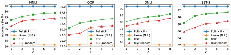
Figure 4: Prediction accuracy of BERT on downstream tasks with varying $\epsilon$. For MNLI, we plot the average score of two test datasets.

Table 4: Prediction accuracy of BERT on downstream tasks (in %). For DP-SGD, RGP, and RGP-random, a same $\epsilon=8$ is used.

Method	MNLI	QQP	QNLI	SST-2	Avg.
Full (N.P.)	84.8/83.7	90.2	91.6	93.4	88.7
Linear (N.P.)	51.9/50.8	73.2	63.0	82.1	64.2
RGP (N.P.)	83.6/83.2	89.3	91.3	92.9	88.1
DP-SGD	54.6/53.4	74.5	63.6	82.3	65.7
RGP-random	74.6/73.3	81.7	82.1	87.8	79.9
RGP	79.1/78.0	84.8	86.2	91.5	83.9

5.3 Defense Against Membership Inference Attack

Setup. We use membership inference (MI) attack to empirically evaluate the privacy risk of models trained with/without RGP. Following the membership decision in Sablayrolles et al. (2019), we predict a sample from the training data if its loss value is smaller than a chosen threshold. To evaluate the MI success rate, we construct a MI dataset, which consists of the same number of training and test samples. Specifically, the MI dataset contains the whole test set and a random subset of the training set. We further divide the MI dataset evenly into two subsets. One is used to find the optimal loss threshold and the other one is used to evaluate the final attack success rate.

Results. The MI success rates are presented in Table 5. For MNLI, QQP, QNLI, and SST-2 datasets, we conduct MI attacks on fine-tuned BERT_BASE models. For SVHN and CIFAR10 datasets, we conduct MI attacks on trained WRN28-4 models. The MI attack on the models trained with RGP ($\epsilon=8$) is no better than random guessing ($50\%$ success rate), which empirically demonstrate the effectiveness of RGP in protecting privacy. Moreover, interestingly, the models trained with low-rank reparametrization alone also achieve much lower MI success rate than the fully trained model, which indicates the benefit of low-rank reparametrization in terms of privacy protection.

6 Related Work

Table 5: Success rates of membership inference attack against fine-tuned BERT models (in %). The closer to 50, the better.

Method MNLI QQP QNLI SST-2 SVHN CIFAR10 Full (N.P.) 60.3 56.1 55.8 57.7 56.4 58.1 RGP (N.P.) 52.3 51.5 51.8 52.6 52.8 53.3 RGP ($\epsilon=8$) 49.9 50.0 50.4 50.1 50.1 50.3

Differentially private learning has a poor dimensional dependency, i.e., the utility degrades dramatically when the model dimension gets large. In the high-dimensional setting, related works usually assume the sparse structure (Thakurta & Smith, 2013; Talwar et al., 2015; Wang & Xu, 2019; Wang et al., 2019a; Cai et al., 2019) or specific problem structure (Chen et al., 2020; Zheng et al., 2020). However, these assumptions or specific structures do not hold for the gradient of deep neural networks. Here we emphasize the difference from our low-rank assumption. For the sparsity assumption, the bases are canonical and not private while for the low-rank assumption, it is “sparse” under certain bases but the bases are unknown and private. Hence the previous algorithms for sparsity cannot apply here.

Very recently, several works (Zhou et al., 2020; Kairouz et al., 2020; Yu et al., 2021a) exploit the redundancy of gradients of samples and suggest projecting the gradients into a low dimensional subspace that is identified by some public data points or historical gradients, in order to reduce the noise effect when training large models. However, they all require storing and clipping whole individual gradients and hence are hard to train extremely large models. Our work is orthogonal with theirs, i.e., we exploit the low-rank property of the gradient of each weight matrix, which truly breaks the barrier of applying DP in large models.

Another recent approach of training non-convex models with differential privacy is based on the knowledge transfer of machine learning models Private Aggregation of Teacher Ensembles (PATE) (Papernot et al., 2017, 2018; Jordon et al., 2019). They first train independent teacher models on disjoint shards of private data and then tune a student model with privacy by distilling noisy predictions of teacher models on some public samples, whose performance suffers from the data splitting (Yu et al., 2021a). It is not clear how to apply PATE to train large language models like BERT. In contrast, our algorithms do not require public data and can be used in different settings with little change.

The phenomenon that the gradients of deep models live on a very low dimensional manifold has been widely observed (Gur-Ari et al., 2018; Vogels et al., 2019; Gooneratne et al., 2020; Li et al., 2020; Martin & Mahoney, 2018; Li et al., 2018). People have also used this fact to compress the gradient with low-rank approximation in the distributed optimization scenario (Yurtsever et al., 2017; Wang et al., 2018b; Karimireddy et al., 2019; Vogels et al., 2019).

7 Conclusion

In this paper, we present the reparametrized gradient perturbation (RGP) for applying DP on large models. The key design of RGP exploits two properties of gradients in deep neural network, which are 1) the gradient of each weight matrix is of low stable rank, 2) the principal components of historical gradients align well with that of the current gradient. We also justify the designs with both theoretical and empirical evidence. Thanks to RGP, we are able to train BERT on several downstream tasks with DP guarantee and achieve small accuracy loss.

Appendix A Preliminary on Differential Privacy

Differential privacy (DP) (Dwork et al., 2006, 2014b) is widely recognized as a gold standard of privacy protection due to its mathematical rigor. It controls the maximum influence that any individual sample can produce. The definition of $(\epsilon,\delta)$-DP is given in Definition 1.

Definition 1 ($(\epsilon,\delta)$-DP).

A randomized mechanism $\mathcal{M}$ guarantees $(\epsilon,\delta)$-differential privacy if for any two neighboring input datasets ${\mathbb{D}}\sim{\mathbb{D}}^{{}^{\prime}}$ and for any subset of outputs ${\mathbb{S}}$ it holds that $\text{Pr}[\mathcal{M}({\mathbb{D}})\in{\mathbb{S}}]\leq e^{\epsilon}\text{Pr}[\mathcal{M}({\mathbb{D}}^{{}^{\prime}})\in{\mathbb{S}}]+\delta$.

Two datasets are said to be neighboring datasets if they only differ in a single sample. When being applied to learning problems, DP requires the learned models on neighboring datasets have approximately indistinguishable distributions.

Appendix B Missing Proofs

B.1 Missing Proofs in Section 2

See 2.1

Proof.

The proof is based on the chain rule of back-propagation. Since the reparametrization does not change the forward and backward signals, we assume the layer inputs are ${\mathbb{D}}=\{{\bm{x}}_{i}\}_{i=1}^{m}$, the corresponding outputs are $\{{\bm{h}}_{i}\}_{i=1}^{m}$ with ${\bm{h}}_{i}={\bm{W}}{\bm{x}}_{i}$ and the backward signals on the layer output are $\{\partial{\bm{h}}_{i}\}_{i=1}^{m}$. By back-propagation, we have

$$\partial{\bm{W}}=\sum_{{\bm{x}}_{i}\in{\mathbb{D}}}(\partial{\bm{h}}_{i}){\bm{x}}_{i}^{T},$$

$$\partial{\bm{L}}=\sum_{{\bm{x}}_{i}\in{\mathbb{D}}}\partial{\bm{h}}_{i}({\bm{R}}{\bm{x}}_{i})^{T},\;\;\partial{\bm{R}}=\sum_{{\bm{x}}_{i}\in{\mathbb{D}}}({\bm{L}}^{T}\partial{\bm{h}}_{i}){\bm{x}}_{i}^{T}.$$

Proof is completed by the multiplication associativity. ∎

See 2.1.1

Proof.

If the columns of ${\bm{L}}$ and the rows of ${\bm{R}}$ are orthonormal, the projection of $\partial{\bm{W}}$ onto ${\bm{L}}$ and ${\bm{R}}$ is defined as,

$${\bm{L}}{\bm{L}}^{T}(\partial{\bm{W}})+(\partial{\bm{W}}){\bm{R}}^{T}{\bm{R}}-{\bm{L}}{\bm{L}}^{T}(\partial{\bm{W}}){\bm{R}}^{T}{\bm{R}}.$$ (10)

Substituting the above formula with $\partial{\bm{L}}=(\partial{\bm{W}}){\bm{R}}^{T}$ and $\partial{\bm{R}}={\bm{L}}^{T}(\partial{\bm{W}})$ in Theorem 2.1, completes the proof. ∎

B.2 Missing Proofs in Section 3

See 3.1

Proof.

Although RGP releases projected gradient instead of releasing the whole gradient as in Abadi et al. (2016), moments accountant is still applicable because it applies to vectorized function output.

Moments accountant tracks a bound on the moments of the privacy loss random variable, which is built on the ratio of the probability density functions of the output distributions of two neighboring datasets. Abadi et al. (2016) show the log moments of the privacy loss random variable composes linearly. Therefore one can compute the overall privacy cost by adding the log moments at every update. When the training is done, moments accountant casts the accumulated log moments into $(\epsilon,\delta)$-DP via tail bound. Detailed proof can be found in Appendix B of Abadi et al. (2016).

∎

B.3 Missing Proofs in Section 4

See 4.1

Proof.

We can compute the gradient at step $t$

$$\partial{\bm{W}}_{t} =\frac{1}{n}\sum_{i=1}^{n}({\bm{W}}_{t}{\bm{x}}_{i}-{\bm{y}}_{i}){\bm{x}}_{i}^{T}.$$

Given the gradient descent update equation 8, we can compute the gradient at ${\bm{W}}_{t+1}$ as follows

$$\partial{\bm{W}}_{t+1} =\frac{1}{n}\sum_{i=1}^{n}(({\bm{W}}_{t}-\eta\cdot\partial{\bm{W}}_{t}){\bm{x}}_{i}-{\bm{y}}_{i}){\bm{x}}_{i}^{T}$$

$$=\frac{1}{n}\sum_{i=1}^{n}({\bm{W}}_{t}{\bm{x}}_{i}-{\bm{y}}_{i}){\bm{x}}_{i}^{T}-\eta\cdot\partial{\bm{W}}_{t}\sum_{i=1}^{n}{\bm{x}}_{i}{\bm{x}}_{i}^{T}$$

$$=\partial{\bm{W}}_{t}\left({\bm{I}}-\eta\sum_{i=1}^{n}{\bm{x}}_{i}{\bm{x}}_{i}^{T}\right).$$

Hence we have $\partial{\bm{W}}_{t}=\partial{\bm{W}}_{0}\left({\bm{I}}-\eta\sum_{i=1}^{n}{\bm{x}}_{i}{\bm{x}}_{i}^{T}\right)^{t}$. The $\partial{\bm{W}}_{t}$ lives in the same subspace for all $t\geq 1$ as they have the same row/column spaces. ∎

Appendix C Additional Experiments

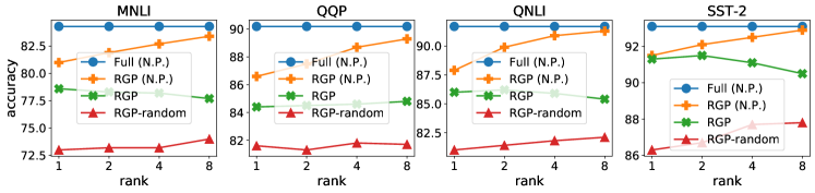
Figure 5: Prediction accuracy of BERT on four downstream tasks (in %) with difference choices of reparametrization rank. We plot the average score of two test datasets for MNLI.

We present some ablation studies in this section to verify the effect of residual weight and reparametrization rank. In Section C.1, we try RGP with difference rank choices. In Section C.2, we give a variant of RGP that simply discards the residual weight.

C.1 On the Influence of Different Rank Choices

We present the results (see Figure 5) with different choices of reparametrization rank. We consider four algorithms. The first one is fine-tuning the full model that serves as the baseline. The second one is RGP (N.P.) that trains the model with reparametrization but without gradient clipping or adding noise. The third one is RGP (Algorithm 1) and the last one is RGP-random, which uses random orthogonal vectors as gradient-carrier matrices. The privacy parameter $\epsilon$ is $8$ and other settings are the same as those in Section 5. The results are plotted in Figure 5. When the models are trained without noise, increasing the reparametrization rank makes the performance of RGP (N.P.) approach the performance of baseline. When the models are trained with privacy guarantee, increasing the rank sometimes decreases the performance because a larger rank induces more trainable parameters and hence higher noise dimension.

C.2 On the Importance of Residual Weight

Recall that our reparametrization scheme reparametrizes the weight matrix as follows:

$${\bm{W}}\rightarrow{\bm{L}}{\bm{R}}+\tilde{{\bm{W}}}.{stop\_gradient()}.$$ (11)

We have shown that the residual weight $\tilde{{\bm{W}}}$ keeps the forward/backward signals unchanged and makes the gradients of ${\bm{L}}$ and ${\bm{R}}$ naturally connected with the original gradient. To empirically examine the effect of $\tilde{{\bm{W}}}$, we test the following scheme:

$${\bm{W}}\rightarrow{\bm{L}}{\bm{R}}.$$ (12)

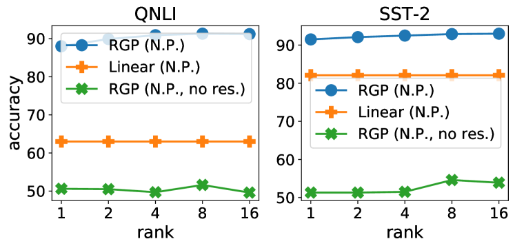
Figure 6: Prediction accuracy of BERT on two downstream tasks. All methods are trained without privacy guarantee.

We still use the historical update to generate ${\bm{L}}$ and ${\bm{R}}$. Other settings are the same as those in Section 5. The results on two downstream tasks of the BERT model are presented in Figure 6. Without residual weight, the model learns almost nothing from the re-constructed update and the final accuracy is close to the accuracy at initialization.

References

- Abadi et al. (2016) Abadi, M., Chu, A., Goodfellow, I., McMahan, H. B., Mironov, I., Talwar, K., and Zhang, L. Deep learning with differential privacy. In ACM SIGSAC Conference on Computer and Communications Security, 2016.
- Agarwal et al. (2018) Agarwal, N., Suresh, A. T., Yu, F. X. X., Kumar, S., and McMahan, B. cpsgd: Communication-efficient and differentially-private distributed sgd. In Advances in Neural Information Processing Systems, 2018.
- Balles & Hennig (2018) Balles, L. and Hennig, P. Dissecting adam: The sign, magnitude and variance of stochastic gradients. In International Conference on Machine Learning, 2018.
- Balles et al. (2016) Balles, L., Romero, J., and Hennig, P. Coupling adaptive batch sizes with learning rates. arXiv preprint arXiv:1612.05086, 2016.
- Bassily et al. (2014) Bassily, R., Smith, A., and Thakurta, A. Differentially private empirical risk minimization: Efficient algorithms and tight error bounds. Annual Symposium on Foundations of Computer Science, 2014.
- Bernau et al. (2019) Bernau, D., Grassal, P.-W., Robl, J., and Kerschbaum, F. Assessing differentially private deep learning with membership inference. arXiv preprint arXiv:1912.11328, 2019.
- Cai et al. (2019) Cai, T. T., Wang, Y., and Zhang, L. The cost of privacy: Optimal rates of convergence for parameter estimation with differential privacy. arXiv preprint arXiv:1902.04495, 2019.
- Carlini et al. (2019) Carlini, N., Liu, C., Erlingsson, Ú., Kos, J., and Song, D. The secret sharer: Evaluating and testing unintended memorization in neural networks. In USENIX Security Symposium, 2019.
- Carlini et al. (2020) Carlini, N., Tramer, F., Wallace, E., Jagielski, M., Herbert-Voss, A., Lee, K., Roberts, A., Brown, T., Song, D., Erlingsson, U., et al. Extracting training data from large language models. arXiv preprint arXiv:2012.07805, 2020.
- Chaudhuri & Monteleoni (2009) Chaudhuri, K. and Monteleoni, C. Privacy-preserving logistic regression. In Advances in Neural Information Processing Systems, 2009.
- Chen et al. (2020) Chen, X., Zheng, K., Zhou, Z., Yang, Y., Chen, W., and Wang, L. (Locally) differentially private combinatorial semi-bandits. In Proceedings of the 37th International Conference on Machine Learning, pp. 1757–1767. PMLR, 13–18 Jul 2020.
- Dangel et al. (2019) Dangel, F., Kunstner, F., and Hennig, P. Backpack: Packing more into backprop. In International Conference on Learning Representations, 2019.
- Devlin et al. (2018) Devlin, J., Chang, M.-W., Lee, K., and Toutanova, K. Bert: Pre-training of deep bidirectional transformers for language understanding. arXiv preprint arXiv:1810.04805, 2018.
- Dwork et al. (2006) Dwork, C., McSherry, F., Nissim, K., and Smith, A. Calibrating noise to sensitivity in private data analysis. In Theory of cryptography conference, 2006.
- Dwork et al. (2014a) Dwork, C., Roth, A., et al. The algorithmic foundations of differential privacy. Foundations and Trends® in Theoretical Computer Science, 2014a.
- Dwork et al. (2014b) Dwork, C., Roth, A., et al. The algorithmic foundations of differential privacy. Foundations and Trends in Theoretical Computer Science, 9(3-4):211–407, 2014b.
- Glorot & Bengio (2010) Glorot, X. and Bengio, Y. Understanding the difficulty of training deep feedforward neural networks. In Proceedings of the Thirteenth International Conference on Artificial Intelligence and Statistics, Proceedings of Machine Learning Research, 2010.
- Gooneratne et al. (2020) Gooneratne, M., Sim, K. C., Zadrazil, P., Kabel, A., Beaufays, F., and Motta, G. Low-rank gradient approximation for memory-efficient on-device training of deep neural network. In IEEE International Conference on Acoustics, Speech and Signal Processing (ICASSP), 2020.
- Gur-Ari et al. (2018) Gur-Ari, G., Roberts, D. A., and Dyer, E. Gradient descent happens in a tiny subspace. arXiv preprint arXiv:1812.04754, 2018.
- He et al. (2016) He, K., Zhang, X., Ren, S., and Sun, J. Deep residual learning for image recognition. In Proceedings of the IEEE conference on computer vision and pattern recognition, 2016.
- Jordon et al. (2019) Jordon, J., Yoon, J., and van der Schaar, M. Pate-gan: Generating synthetic data with differential privacy guarantees. In International Conference on Learning Representations, 2019.
- Kairouz et al. (2020) Kairouz, P., Ribero, M., Rush, K., and Thakurta, A. Dimension independence in unconstrained private erm via adaptive preconditioning. arXiv preprint arXiv:2008.06570, 2020.
- Karimireddy et al. (2019) Karimireddy, S. P., Rebjock, Q., Stich, S., and Jaggi, M. Error feedback fixes signsgd and other gradient compression schemes. In International Conference on Machine Learning, 2019.
- Krizhevsky & Hinton (2009) Krizhevsky, A. and Hinton, G. Learning multiple layers of features from tiny images. 2009.
- Lecuyer et al. (2019) Lecuyer, M., Atlidakis, V., Geambasu, R., Hsu, D., and Jana, S. Certified robustness to adversarial examples with differential privacy. In 2019 IEEE Symposium on Security and Privacy (S&P), 2019.
- Li et al. (2020) Li, X., Gu, Q., Zhou, Y., Chen, T., and Banerjee, A. Hessian based analysis of sgd for deep nets: Dynamics and generalization. In SIAM International Conference on Data Mining, 2020.
- Li et al. (2021) Li, X., Tramèr, F., Liang, P., and Hashimoto, T. Large language models can be strong differentially private learners. arXiv preprint arXiv:2110.05679, 2021.
- Li et al. (2018) Li, Y., Ma, T., and Zhang, H. Algorithmic regularization in over-parameterized matrix sensing and neural networks with quadratic activations. In Conference On Learning Theory, 2018.
- Ma et al. (2019) Ma, Y., Zhu, X., and Hsu, J. Data poisoning against differentially-private learners: attacks and defenses. In Proceedings of the 28th International Joint Conference on Artificial Intelligence, 2019.
- Mahsereci & Hennig (2017) Mahsereci, M. and Hennig, P. Probabilistic line searches for stochastic optimization. The Journal of Machine Learning Research, 2017.
- Martin & Mahoney (2018) Martin, C. H. and Mahoney, M. W. Implicit self-regularization in deep neural networks: Evidence from random matrix theory and implications for learning. arXiv preprint arXiv:1810.01075, 2018.
- Mironov et al. (2019) Mironov, I., Talwar, K., and Zhang, L. Rényi differential privacy of the sampled gaussian mechanism. arXiv, 2019.
- Netzer et al. (2011) Netzer, Y., Wang, T., Coates, A., Bissacco, A., Wu, B., and Ng, A. Y. Reading digits in natural images with unsupervised feature learning. 2011.
- Opacus (2020) Opacus. Pytorch opacus project, 2020. URL https://github.com/pytorch/opacus.
- Papernot et al. (2017) Papernot, N., Abadi, M., Erlingsson, U., Goodfellow, I., and Talwar, K. Semi-supervised knowledge transfer for deep learning from private training data. 2017.
- Papernot et al. (2018) Papernot, N., Song, S., Mironov, I., Raghunathan, A., Talwar, K., and Erlingsson, Ú. Scalable private learning with pate. 2018.
- Papernot et al. (2020) Papernot, N., Thakurta, A., Song, S., Chien, S., and Erlingsson, Ú. Tempered sigmoid activations for deep learning with differential privacy. arXiv preprint arXiv:2007.14191, 2020.
- Phan et al. (2020) Phan, H., Thai, M. T., Hu, H., Jin, R., Sun, T., and Dou, D. Scalable differential privacy with certified robustness in adversarial learning. In International Conference on Machine Learning, 2020.
- Rahman et al. (2018) Rahman, M. A., Rahman, T., Laganiere, R., Mohammed, N., and Wang, Y. Membership inference attack against differentially private deep learning model. Transactions on Data Privacy, 2018.
- Sablayrolles et al. (2019) Sablayrolles, A., Douze, M., Ollivier, Y., Schmid, C., and Jégou, H. White-box vs black-box: Bayes optimal strategies for membership inference. International Conference on Machine Learning, 2019.
- Shokri et al. (2017) Shokri, R., Stronati, M., Song, C., and Shmatikov, V. Membership inference attacks against machine learning models. In IEEE Symposium on Security and Privacy (SP), 2017.
- Song et al. (2013) Song, S., Chaudhuri, K., and Sarwate, A. D. Stochastic gradient descent with differentially private updates. In Global Conference on Signal and Information Processing (GlobalSIP), 2013.
- Talwar et al. (2015) Talwar, K., Thakurta, A. G., and Zhang, L. Nearly optimal private lasso. In Advances in Neural Information Processing Systems, 2015.
- Thakurta & Smith (2013) Thakurta, A. G. and Smith, A. Differentially private feature selection via stability arguments, and the robustness of the lasso. In Conference on Learning Theory, 2013.
- Tramèr & Boneh (2021) Tramèr, F. and Boneh, D. Differentially private learning needs better features (or much more data). In International Conference on Learning Representations (ICLR), 2021.
- Vietri et al. (2020) Vietri, G., Balle, B., Krishnamurthy, A., and Wu, S. Private reinforcement learning with pac and regret guarantees. In International Conference on Machine Learning, 2020.
- Vogels et al. (2019) Vogels, T., Karimireddy, S. P., and Jaggi, M. Powersgd: Practical low-rank gradient compression for distributed optimization. In Advances in Neural Information Processing Systems, 2019.
- Wang et al. (2018a) Wang, A., Singh, A., Michael, J., Hill, F., Levy, O., and Bowman, S. R. Glue: A multi-task benchmark and analysis platform for natural language understanding. arXiv preprint arXiv:1804.07461, 2018a.
- Wang & Xu (2019) Wang, D. and Xu, J. On sparse linear regression in the local differential privacy model. In International Conference on Machine Learning, 2019.
- Wang et al. (2019a) Wang, D., Chen, C., and Xu, J. Differentially private empirical risk minimization with non-convex loss functions. In International Conference on Machine Learning, 2019a.
- Wang et al. (2018b) Wang, H., Sievert, S., Liu, S., Charles, Z., Papailiopoulos, D., and Wright, S. Atomo: Communication-efficient learning via atomic sparsification. Advances in Neural Information Processing Systems, 31:9850–9861, 2018b.
- Wang & Gu (2019) Wang, L. and Gu, Q. Differentially private iterative gradient hard thresholding for sparse learning. In International Joint Conference on Artificial Intelligence, 2019.
- Wang et al. (2019b) Wang, Y.-X., Balle, B., and Kasiviswanathan, S. P. Subsampled rényi differential privacy and analytical moments accountant. In International Conference on Artificial Intelligence and Statistics, 2019b.
- Yu et al. (2020) Yu, D., Zhang, H., Chen, W., Yin, J., and Liu, T.-Y. Gradient perturbation is underrated for differentially private convex optimization. In Proc. of 29th Int. Joint Conf. Artificial Intelligence, 2020.
- Yu et al. (2021a) Yu, D., Zhang, H., Chen, W., and Liu, T.-Y. Do not let privacy overbill utility: Gradient embedding perturbation for private learning. In International Conference on Learning Representations, 2021a. URL https://openreview.net/forum?id=7aogOj_VYO0.
- Yu et al. (2021b) Yu, D., Zhang, H., Chen, W., Yin, J., and Liu, T.-Y. How does data augmentation affect privacy in machine learning? In Proc. of the AAAI Conference on Artificial Intelligence, 2021b.
- Yurtsever et al. (2017) Yurtsever, A., Udell, M., Tropp, J. A., and Cevher, V. Sketchy decisions: Convex low-rank matrix optimization with optimal storage. In International Conference on Artificial Intelligence and Statistics (AISTATS), 2017.
- Zagoruyko & Komodakis (2016) Zagoruyko, S. and Komodakis, N. Wide residual networks. arXiv preprint arXiv:1605.07146, 2016.
- Zhao & Zhang (2015) Zhao, P. and Zhang, T. Stochastic optimization with importance sampling for regularized loss minimization. In international conference on machine learning, 2015.
- Zheng et al. (2020) Zheng, K., Cai, T., Huang, W., Li, Z., and Wang, L. Locally differentially private (contextual) bandits learning. In Advances in Neural Information Processing Systems, 2020.
- Zhou et al. (2020) Zhou, Y., Wu, Z. S., and Banerjee, A. Bypassing the ambient dimension: Private sgd with gradient subspace identification. arXiv preprint arXiv:2007.03813, 2020.
- Zhou et al. (2021) Zhou, Y., Wu, S., and Banerjee, A. Bypassing the ambient dimension: Private {sgd} with gradient subspace identification. In International Conference on Learning Representations, 2021. URL https://openreview.net/forum?id=7dpmlkBuJFC.
- Zhu et al. (2019) Zhu, L., Liu, Z., and Han, S. Deep leakage from gradients. In Advances in Neural Information Processing Systems, 2019.