Optimal mean first-passage time of a Brownian searcher with resetting in one and two dimensions: Experiments, theory and numerical tests

Abstract

We study experimentally, numerically and theoretically the optimal mean time needed by a Brownian particle, freely diffusing either in one or two dimensions, to reach, within a tolerance radius $R_{\text{t}ol}$, a target at a distance $L$ from an initial position in the presence of resetting. The reset position is Gaussian distributed with width $\sigma$. We derived and tested two resetting protocols, one with a periodic and one with random (Poissonian) resetting times. We computed and measured the full first-passage probability distribution that displays spectacular spikes immediately after each resetting time for close targets. We study the optimal mean first-passage time as a function of the resetting period/rate for different target distances (values of the ratios $b=L/\sigma$) and target size ($a=R_{\text{tol}}/L$). We find an interesting phase transition at a critical value of $b$, both in one and two dimensions. The details of the calculations as well as experimental setup and limitations are discussed.

I Introduction

The time needed by a freely diffusing Brownian particle to reach a fixed target in space is a widely studied problem not only for its fundamental aspects but also for its numerous applications from chemical reactions, astrophysics, all the way to animal foraging in ecology. This time is a random variable and its probability distribution is called the first-passage time distribution Redner (2001); Bray et al. (2013). The first moment of this distribution, when it exists, is called the mean first-passage time (MFPT) which is often used as a measure of the efficiency of a search process. The smaller the MFPT, the more efficient is the search process. The MFPT can be optimized using various stochastic search algorithms (such as simulated annealing) which speed up the search process Villen-Altramirano and Villen-Altramirano (1991); Luby et al. (1993); Tong et al. (2008); Lorenz (2018). More recently it has been demonstrated that the MFPT for a single particle (searcher) to a fixed target can be minimized using the reset protocols (for a recent review see  Evans et al. (2020)). Searching a target via resetting is an example of the so called intermittent search strategy O et al. (2011) consisting of a mixture of short-range localised moves (where the searcher actually performs the search) with intermittent long-range moves where the searcher moves to a new location and starts a local search in the new place.

Consider, for example, a fixed target at some point in space and a particle (searcher) starts its dynamics from a fixed initial position in space. The dynamics of the particle is represented by a stochastic process, e.g. it may just be simple diffusion Evans and Majumdar (2011a, b). Under resetting protocol, the motion of the searcher is interrupted either randomly at a constant rate $r$ Evans and Majumdar (2011a, b) or periodically with a period $T$ Pal et al. (2016); Bhat et al. (2016), and then the particle is sent back to its initial position (usually instantaneously) and the search restarts again from the initial position after each resetting event. For a given fixed distance between the target and the initial position of the searcher, if one plots the MFPT as a function of the resetting rate $r$ (or $T$ for periodical resetting), the MFPT typically displays a unique minimum at some optimal value $r^{*}$. This led to the paradigm that resetting typically makes the search process more efficient if the resetting rate is chosen to have its optimal value $r^{*}$ Evans and Majumdar (2011a, b).

While this ‘optimal resetting’ paradigm has been tested and verified in a large number of recent theoretical and numerical studies Evans et al. (2013); Montero and Villarroel (2013); Evans and Majumdar (2014); Kuśmierz et al. (2014); Reuveni et al. (2014); Rotbart et al. (2015); Christou and Schadschneider (2015); Kuśmierz and Gudowska-Nowak (2015); Pal et al. (2016); Nagar and Gupta (2016); Reuveni (2016); Pal and Reuveni (2017); Chechkin and Sokolov (2018); Belan (2018); Evans and Majumdar (2018); A. Masó-Puigdellosas and Méndez (2019); Masoliver and Montero (2019); Durang et al. (2019); Pal and Prasad (2019) (see also the review Evans et al. (2020)), it has been been verified only in a few experiments limited to the one dimensional (1D) case Tal-Friedman et al. (2020); Besga et al. (2020). In Ref. Besga et al. (2020) we have demonstrated the emergence of new physical effects when the resetting position is not fixed to be exactly the initial position, but has a distribution of finite width $\sigma$ around an average initial position. A finite value of $\sigma$ led to interesting metastability and phase transition in the MFPT as a function of resetting rate/period. Very recently Besga et al. , we have shown that a finite $\sigma$ in the initial condition also affects, rather profoundly, the first-passage probability distribution of the searcher, even in the absence of resetting.

The purpose of this article is to extend these results to the two dimensional (2D) case, showing both theoretically and experimentally that the new physical effects induced by a nonzero $\sigma$ discussed above are not restricted just to 1D, but are also observed in 2D. Our article is organized as follows. In the next section we describe the experimental set-up and the difficulties that one encounters in performing such experiments. In section III we recall the main experimental results in 1D, whereas the theoretical predictions for 1D are summarized in the Appendices A-C. Although the 1D results have been recently published in a shortened form without details in Ref. Besga et al. (2020), we think that it is useful to recall them with details in this article, in order to have a full comparisons with the 2D results described in Section IV. The details of the 2D theoretical computations, which are rather nontrivial, are provided in the Appendices D and E. We finally conclude in Section V and some further details are relegated to the rest of the Appendices.

II Experimental set-up.

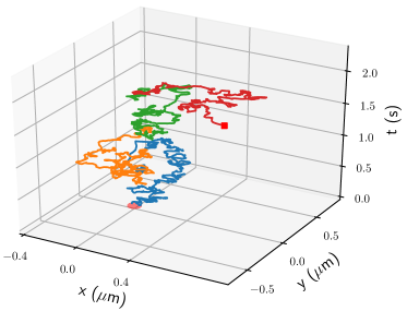
Figure 1: Top panel : Brownian trajectory in the 2D plane $(x,y)$ over time $t$ with resetting. Bottom panel : Corresponding 1D Brownian trajectory with periodic resetting after $T=$0.5\text{\,}\mathrm{s}$$ (red colored area). The equilibrium standard deviation of the trapped particle $\sigma_{x}=$43\text{\,}\mathrm{nm}$$ is shown (dotted lines). The target (red square $1\text{\,}\mathrm{\SIUnitSymbolMicro m}$ away from the center of the trap) is reached when $x$ crosses the red line for the first time.

The optimal search protocol is implemented in an optical tweezer experiment Bèrut et al. (2016). The Brownian searcher is a silica micro-sphere of radius $R=$1\text{\,}\mathrm{\SIUnitSymbolMicro m}$$ ($\pm 5\%$) immersed in pure water. The fluid chamber is made of two parts : The colloids are inserted in the thicker part of the chamber (reservoir) and the measurements are performed in a second part (thickness around $50\text{\,}\mathrm{\SIUnitSymbolMicro m}$) with very few particles which allows us to take long duration measurements (tenths of hours). The optical trap is implemented with a near infrared laser with wavelength $\lambda=$1064\text{\,}\mathrm{nm}$$ focused into the chamber through an oil immersion objective (Leica $63\times$ and $1.4$ NA). The particle is trapped in the transverse plane $(x,y)$ by a harmonic potential with stiffness $\kappa_{x,y}$. The stiffness is controlled by changing the optical power (typically hundreds of mW) in the chamber directly by laser current modulation (up to 10 kHz) or faster using an electro-optical modulator (EOM). The position of the particle in the $(x,y)$ plane can be tracked (see Fig. (1)) either by a white light imaging on a camera or from the deviation of a second laser on a quadrant photodiode (QPD). The camera allows us to extract the position of the bead at maximum speed around 1000 frames per second over a broad range ($>$100\text{\,}\mathrm{\SIUnitSymbolMicro m}$$) and the center of the bead is extracted in real time with an accuracy of $2\text{\,}\mathrm{nm}$. On the other hand the QPD allows for a fast position detection (around $1\text{\,}\mathrm{MHz}$ bandwidth) with a smaller range ($<$1\text{\,}\mathrm{\SIUnitSymbolMicro m}$$) and a better accuracy (below $1\text{\,}\mathrm{nm}$).

We implemented different search protocols (see below) involving a free diffusion phase where the particle actually searches for a target (with duration $T$) and a second phase resetting the particule to an initial distribution ${\cal P}(x_{0},y_{0})$. The resetting is implemented by turning on the optical trap during a time long enough for the particle to equilibrate in the trap. During this equilibration period, we do not make any first-passage measurement. The first passage time is measured when the position crosses, during the diffusive phase, the target line in 1D for the first time (see Fig. (1) bottom panel) or when the particle enters for the first time the tolerance radius around the target in 2D (see Fig. (6) in Section IV).

We point out here a few difficulties encountered in such experiments. First the free diffusion phase cannot be too long (typically $T<$1\text{\,}\mathrm{s}$$) to prevent the particle to diffuse too far from the center of the trap, as it needs to get trapped again in the next resetting phase. It is also important to make measurements close to the bottom surface of the chamber to avoid errors in position reading due to sedimentation during the free diffusion phase. Finally the acquisition rate has to be high enough to detect fast events (see discussion in Section III).

We will first discuss periodic and poissonian protocols in the 1D case in the next Section, where we focus only on the $x$-component of the particle’s position, i.e., one dimensional trajectories. Later, in Section IV, we will analyse the full 2D trajectories in detail.

III The optimal resetting protocols in one dimension

III.1 Periodic resetting protocol.

The experimental protocol leads us to study a model of diffusion in (effectively) one dimension subjected to periodic resetting. We consider an overdamped particle in thermal equilibrium inside a harmonic trap with potential $U(x)=\kappa\,x^{2}/2$, where the stiffness $\kappa$ is proportional to the trapping laser power. The particle is allowed to equilibrate in the trap, and once it has acheived thermal equilibrium, the time is switched on. This means that the initial position $x_{0}$ is distributed via the Gibbs-Bolzmann distribution which is simply Gaussian in a harmonic trap: ${\cal P}(x_{0})=\mathrm{e}^{-x_{0}^{2}/2\sigma^{2}}/\sqrt{2\pi\sigma^{2}}$ with width $\sigma=\sqrt{k_{B}{\cal T}/\kappa}$, where ${\cal T}$ is the temperature. We also set a a fixed target at location $L$.

At time $t=0$, the trap is switched off for an interval $T$ and the particle undergoes free diffusion (overdamped) with diffusion constant $D=k_{B}{\cal T}/\Gamma$, where $\Gamma$ is the friction coefficient. At the end of the period $T$, the particle’s position is reset (see Fig. (1)). Performing the resetting of the position poses the real experimental challenge.

In standard models of resetting one usually assumes instantaneous resetting Evans et al. (2020), which is however impossible to achieve experimentally. In our experiment, the resetting is done by allowing the particle to relax to its thermal equilibrium in the trap. This poses two problems.

• First, there is always a finite relaxation time needed for the particle to reset or equilibrate (it is never instantaneous as in the theoretical models). There have been recent theoretical studies of resetting protocols with a finite ‘refraction’ period needed to reset the particle to its initial postion Reuveni (2016); Evans and Majumdar (2019); A. Masó-Puigdellosas and Méndez (2019); Pal et al. (2019); Gupta et al. (2020); Bodrova and Sokolov (2020); Mercado-Vásquez et al. (2020); Gupta et al. (2021). In our experiment, the analogue of this refraction period is the relaxation time to equilibrium once the trap is switched on after the period $T$ of free diffusion. However, since the theoretical calculations are much easier for the instantaneous resetting case Evans et al. (2020), it would be easier to compare the experiments with theory if we can devise an experimental set-up that mimics the ‘instantaneous’ resetting. To devise such a set-up, we first note that the relaxation inside the trap can, in principle, be made arbitrarily fast using, e.g., the recently developed "Engineered Swift Equilibration" (ESE) technique Martínez et al. (2016); Chupeau et al. (2018); Guery-Odelin et al. (2019); C. A. Plata and Prados (2019); Gupta et al. (2020). In our experiment we determine the characteristic relaxation time inside the trap $\tau_{c}=\Gamma/\kappa$. During the period $[T,T+\tau_{\rm eq}]$ with $\tau_{\rm eq}\simeq 3\,\tau_{c}$, we do not make any measurement. In other words, even if the particle encounters the target during this relaxation period, we do not count this as a first-passage event. Thus in this set-up, the thermal relaxation mimics the instantaneous resetting.

• Secondly, while the set-up described above achieves ‘instantaneous’ resetting, it still has one important ingredient that differs from theoretical models of instantaneous resetting. Using this relaxation technique we do not reset it to exactly the same initial position, rather the new ‘initial’ position, at the end of the time epoch $T+\tau_{\rm eq}$, is drawn from the Gibbs-Boltzmann distribution ${\cal P}(x_{0})$. Thus it is important to modify the theoretical results for instantaneous resetting by taking into acount a finite spread $\sigma$ of the resetting position. One of our main results in this paper is to provide new analytical calculations that take into acount the finite $\sigma$ effect on the optimization of the MFPT.

To complete our protocol using the two caveats mentioned above, at time $T+\tau_{\rm eq}$, we again switch off the trap and we let the particle diffuse freely for another period $T$, followed by the thermal relaxation over period $\tau_{\rm eq}$. The process repeats periodically. During the free diffusion, if the particle finds the target at $L$, we count it as a first-passage event and measure this first-passage time $t_{\text{f}}$. Note that the first-passage time $t_{\text{f}}$ is the total ‘diffusion’ time spent by the particle before reaching the target (not counting the intermediate relaxation periods $\tau_{\rm eq}$). Averaging over many realizations, we then compute the MFPT $\langle t_{\text{f}}\rangle$, for fixed target location $L$ and fixed resetting period $T$. As mentioned before, we find that a finite $\sigma$ affects the results for MFPT as a function of the period $T$ in a significant way, leading to new physical phenomena such as metastability and dynamical phase transition which do not exist when $\sigma=0$ strictly.

Mean first-passage time. We start with the MFPT, the central object of our interest. The MFPT for this protocol can be computed analytically, as detailed in Appendix B. Our main result can be summarized in terms of two dimensionless quantities

$$b=\frac{L}{\sigma}\,;\quad{\rm and}\quad c=\frac{L}{\sqrt{4\,D\,T}}\,.$$ (1)

The parameter $b$ quantifies how far the target is from the center of the trap in units of the trapped equilibrium standard deviation. The second parameter $c$ tells us how frequently we reset the particle compared to its free diffusion time. We show that the dimensionless MFPT $\tau$ can be expressed as a function of these two parameters $b$ and $c$ (see Eq. (30) in Appendix B)

$$\tau=\frac{4D\langle t_{\text{f}}\rangle}{L^{2}}=w(b,c)\,,$$ (2)

where

$$w(b,c)=\frac{\int_{0}^{1}\ dv\ \int_{-\infty}^{\infty}\ du\ \mathrm{e}^{(-u^{2}/2)}\ {\rm erf}\left(\frac{c}{\sqrt{v}}\ |1-u/b|\right)}{c^{2}\ \int_{-\infty}^{\infty}\ du\ \mathrm{e}^{(-u^{2}/2)}\operatorname{erfc}\left(c\ |1-u/b|\right)}$$ (3)

While it is hard to evaluate the integrals explicitly, $w(b,c)$ can be easily plotted numerically to study its dependence on $b$ and $c$. Furthermore, one can also evaluate the function $w(b,c)$ explicitly in different limiting cases.

To analyse the MFPT, we start with the limit $b\gg 1$ of Eq. (3), i.e., $L\gg\sigma$. This limit corresponds to the case when the target is much farther away compared to the typical fluctuation of the initial position. In this case, taking $b\to\infty$ limit in Eq. (3) we get

$$w(c)=w(b\to\infty,c)=\frac{{\rm erf}(c)+2c\left(\mathrm{e}^{-c^{2}}/\sqrt{\pi}-c\,{\rm erfc}(c)\right)}{c^{2}\,{\rm erfc}(c)}\,,$$ (4)

where ${\rm erf}(c)=(2/\sqrt{\pi})\,\int_{0}^{c}\mathrm{e}^{-u^{2}}\,du$ and ${\rm erfc}(c)=1-{\rm erf}(c)$. In Fig. (2), we plot $w(c)$ vs $c$ and compare with our experimental data and find good agreement with no adjustable parameter. Typically, to have a good estimate of the MFPT, we follow the particle for a few hours which allows us to detect between 1000 and 10000 first passage times, depending on the values of $b$ and $c$. The standard deviation of first-passage times is of the same order as the MFPT. We see a distinct optimal value around $c^{*}=0.74$, at which $w(c^{*})=5.3$. Our results thus provide a clear experimental verification of the optimal resetting paradigm. Let us remark that the authors in Ref. Pal et al. (2016) studied periodic resetting to the fixed initial position $x_{0}=0$ and obtained the MFPT by a different method than ours. Our $b\to\infty$ limit result in Eq. (4) indeed coincides with that of  Pal et al. (2016), since when $\sigma\ll L$, our protocol mimics approximately a resetting to the origin.

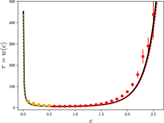
Figure 2: $w(c)\equiv w(b\to\infty,c)$ vs. $c$ curve (see also Fig. (3)). The solid black line represents the theoretical formula for $w(c)$ in Eq. (4), while the dots denote the experimental data with $b=30$ (red dots) and $b=5$ (yellow square). The dotted lines shows $w(b,c)$ with $b=5$ for small $c$ ($c\leq 0.6$) in yellow, and with $b=30$ for higher $c$ in red. The error bars are given by the standard deviation of the MFPT distribution divided by the square root of the number of events.

What happens when $b=L/\sigma$ is finite? Remarkably, when we plot $w(b,c)$ in Eq. (3) as a function of $c$ for different fixed values of $b$, we see that $w(b,c)$ decreases as $c$ increases, indeed achieves a minimum at $c_{1}(b)$, then increases again, achieves a maximum at $c_{2}(b)$ and then decreases monotonically as $c$ increases beyond $c_{2}(b)$ (see Fig. (3)). When $b\to\infty$, the maximum at $c_{2}(b)\to\infty$ and one has a single minimum at $c=c_{1}(b)$ as in Fig. (2). However, for finite $b$, the “optimal” (minimal) MFPT at $c=c_{1}(b)$ is thus actually a ‘metastable’ minimum and the true minimum occurs at $c\to\infty$, i.e., when the resetting period $T\to 0$. Physically, the limit $T\to 0$, i.e., $c\to\infty$ corresponds to repeated (almost continuous) resetting and since the target position and the initial location are of the same order, the particle finds the target very quickly simply by resetting, without the need to diffuse. This explains the second minimum at $c\to\infty$. Interestingly, this metastable minimum at $c=c_{1}(b)$ exists only for $b>b_{c}\approx 2.3$. When $b<b_{c}$, the curve $w(b,c)$ decreases monotonically with $c$ and there is only a single minimum at $c\to\infty$, or equivalently for $T\to 0$. Thus the system undergoes a ‘dynamical’ phase transition as the parameter $b=L/\sigma$ is tuned across a critical value $b_{c}\approx 2.3$, from a phase with a metastable minimum at a finite $c=c_{1}(b)$ to one where the only minimum occurs at $c\to\infty$. This phase transition is well reproduced by the experimental data points. The deviation from theoretical prediction for high values of c is due to the limited experimental acquisition rate (here $50000$ Hz) that prevents us from detecting very fast events and thus leads to an overestimation of the MFPT as confirmed by our numerical simulations.

This phase transition was rather unexpected and came out as a surprise. In a recent paper Besga et al. , we have shown that a similar dynamical phase transition already occurs in the first-passage probability density of a diffusing particle without resetting, when averaged over the initial condition drawn from a distribution ${\cal P}(x_{0})$ with a finite width $\sigma$. Indeed, the transition that we observe in the $w(b,c)$ curve in Fig. (3) also has its origin in the finiteness of $\sigma$. It can be traced back to the fact that there are two time scales in the system when $\sigma$ is finite, namely $T_{1}\sim\mathcal{O}(L^{2}/D)$ and $T_{2}\sim\mathcal{O}(\sigma^{2}/D)$. In terms of the parameter $c=L/\sqrt{4DT}$, they correspond respectively to $c_{1}(b)\sim L/\sqrt{4DT_{1}}\sim\mathcal{O}(1)$ and $c_{2}(b)\sim L/\sqrt{4DT_{2}}\sim L/\sigma\sim b$. When $b\gg 1$ is large, $c_{1}(b)\ll c_{2}(b)$. However, as $b$ decreases, the two times scales approach each other or equivalently, as a function of $c$, the minimum at $c_{1}(b)$ approaches the maximum at $c_{2}(b)$ in Fig. (3). Finally, at a critical value $b_{c}$, the two time scales merge with each other and for $b<b_{c}$, the function $w(b,c)$ decreases monotonically with increasing $c$ with a single minimum at $c\to\infty$. The phase transition is ‘dynamical’ in the sense that it arises when two time scales merge with each other.

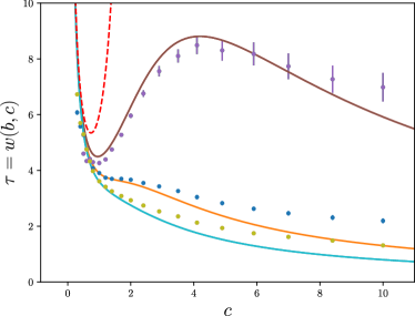
Figure 3: The scaled MFPT $\tau=w(b,c)$ vs. $c$ curves and experimental data for $b=3$ (brown curve and purple dots), $b=2.3$ (orange curve and blue dots) and $b=2$ (blue curve and yellow dots) , for the periodic resetting protocol. The dotted curve recalls the $b\to\infty$ limit. The theoretical curves are obtained from Eq. (3). The scaled MFPT has two different behavior depending on how far is the target. If $b>b_{c}\approx 2.3$ the MFPT $\tau$ exhibits a local minimum, whereas it decreases monotonically for $b$ lower than the critical value $b_{c}$.

The full distribution of the first-passage time. Going beyond the first moment $\langle t_{\text{f}}\rangle$ and computing the full probability density function (PDF) of the first-passage time $t_{\text{f}}$ is also of great interest Majumdar (1999); Redner (2001); Majumdar (2010); Bray et al. (2013). Indeed, we computed the PDF $F(t)$ of $t_{\text{f}}$ (see Appendix C) and the result is plotted in Fig. (4). For small $b$, we found striking spikes in $F(t)$ just after each resetting event. We show in Appendix C that setting $t=n\,T+\Delta$ with $n=0,\,1,\,2\ldots$ and $\Delta\to 0^{+}$, the first-passage density $F(t=n\,T+\Delta)$ displays a power law divergence (the spikes) as $\Delta\to 0^{+}$

$$F(t=n\,T+\Delta)\simeq A_{n}(b)\,\Delta^{-1/2}$$ (5)

with an amplitude $A_{n}(b)$ that can be computed explicitly (see Appendix C). We find that as $b$ increases, $A_{n}(b)$ decays rapidly and the spikes disappear for large $b=L/\sigma$ (see the inset of Fig. (4)). Instead for large $b$, $F(t)$ drops by a finite amount after each period (as seen in the inset). In theoretical models of resetting to a fixed initial position ($\sigma=0$ or $b\to\infty$), these spikes are completely absent and hence they are characteristic of the finiteness of the width $\sigma$ of the resetting position ${\cal P}(x_{0})$.

Figure 4: Experimental (blue histogram) and theoretical (red line) PDF $F(t)$ of the first-passage time. We measured $1.2\times 10^{4}$ first-passage times for $b=2$ and $c=1$ ($T=8.6$ ms). The spikes occur just immediately after $t=n\,T$ where $n=0,\,1,\,2,\ldots$. Inset: The PDF $F(t)$ vs. $t$ (theoretical) for $b=2.2$ to $2.8$ at $c=b/2$ (i.e $T$ constant) that demonstrates that the spikes disappear rapidly with increasing $b$. The PDF $F(t)$ is normalized such that $\int_{0}^{\infty}F(t)d{t}=1$ with $d{t}=3.5\ 10^{-4}$s.

In order to test experimentally these results we realized a periodic resetting protocol and measure the statistics of first-passage times. The diffusion coefficient (typically $D\simeq$2\text{⋅}{10}^{-13}\text{\,}\mathrm{m}^{2}\mathrm{/}\mathrm{s}$$) is measured during the free diffusion part and the width of the Gaussian (typically $\sigma\simeq 40$ nm) when the particle is back to equilibrium. These independent and simultaneous measures allow us to overcome experimental drifts which may appear. In Fig. (4) we show the experimentally obtained PDF of $10^{4}$ measured first-passage times for $b=2$ and $c=1$. We also compared with our theoretical prediction (see Appendix C). We observe a very good agreement with no free parameter.

III.2 Poissonian resetting protocol.

It turns out that this metastability and the phase transition is rather robust and exists for other protocols, such as Poissonian resetting where the resetting occurs at random times (as opposed to periodically in the previous protocol) with a constant rate $r$. Here, the associated dimensionless variables are

$$b=\frac{L}{\sigma}\,;\quad{\rm and}\quad c=\frac{\sqrt{r}L}{\sqrt{D}}\,.$$ (6)

The scaled MFPT $\tau=4D\langle t_{\text{f}}\rangle/L^{2}$ again becomes a function $w_{2}(b,c)$ of $b$ and $c$ (analogue of Eq. (3)). In this case, we get a long but explicit $w_{2}(b,c)$ (see Eq. (48) in Appendix C for details). In Fig. (5) we plot $w_{2}(b,c)$ vs. $c$ for different values of $b$ together with experimental data. We have a good agreement between theory and experiment and here again the deviation at high $c$ comes from limited experimental acquisition rate. Once again we see that there is a metastable minimum that disappears when $b$ decreases below a critical value $b_{c}\approx 2.53$. When $b\to\infty$, there is only a single minimum at $c^{*}=1.59362$ where $w_{2}(\infty,c^{*})=6.17655$. Thus this phenomenon of metastability and phase transition in MFPT seems to be robust.

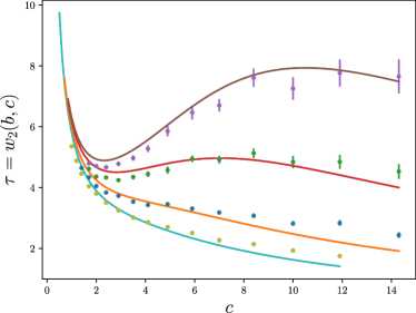
Figure 5: Scaled MFPT $\tau=w_{2}(b,c)$ vs $c$ curves and experimental data points for $b=2,2.3,2.7$ and $3$ (from bottom to top) in the case of Poissonian resetting. The metastable minimum disappears for $b<b_{c}\approx 2.53$.

IV Optimal resetting in 2 dimensions

Figure 6: We consider a searcher in $2$-dimensions starting from an initial position $\vec{r}_{0}$ drawn from the initial distribution centered at the origin, which here is a Gaussian distribution of width $\sigma$. A fixed point target is located at $\vec{R}_{\rm tar}$, with a tolerance radius $R_{\rm tol}$. If the searcher comes within a distance $R_{\rm tol}$ from the target, the target is reached.

In the previous Section we have studied the MFPT with resetting in 1D, both for the periodic and the Poissonian resetting protocols. We now consider a Brownian searcher in 2D, starting initially at the position ${\vec{r}}_{0}$. This position is random, and is drawn from a Gaussian distribution of width $\sigma$. An immobile point target is located at ${\vec{R}}_{\rm tar}$ with a tolerance radius $R_{\rm tol}$ (see Fig. (6)). As the target and the initial position distribution are rotationally invariant, only the target distance $L=|\vec{R}_{\text{tar}}|$ matters. When the searcher comes within the distance $R_{\rm tol}$ from the target at ${\vec{R}}_{\rm tar}$ for the first time, the target is detected and the time at which this occurs is recorded as the first-passage time. A finite tolerance radius is needed in 2D, since a point particle will never find a point target in 2D – making it necessary to have a finite size (cut-off) of the target. This introduces an additional length scale and consequently the analytical calculations are much more involved (see Appendices D and E for the detailed calculations in 2D). In the 2D case, we therefore introduce three dimensionless parameters, to characterize the MFTP $\tau$. Two of these parameters read

$$a=\frac{R_{\rm tol}}{L}<1\,,\quad\,\,b=\frac{L}{\sigma}\,,$$ (7)

where $a$ keeps into account the tolerance radius with respect to the target distance, and $b$ quantifies how far is the target with respect to the spread of the initial distribution as in the 1D case. The third parameter $c$ depends on the protocol: for the periodic protocol with period $T$ and the Poissonian protocol with rate $r$, the parameter $c$ reads respectively

$$c=\frac{L}{\sqrt{4\,D\,T}}\quad\,{\rm and}\quad\,c=\frac{\sqrt{r}\,L}{\sqrt{D}}\,.$$ (8)

The MFPT $\langle t_{\text{f}}\rangle$ for this model is computed analytically in Appendix E. For this, we first computed the survival probability up to time $t$ of a resetting Brownian motion in 2D (with the resetting position chosen from a Gaussian distribution of width $\sigma$) by imposing an absorbing boundary condition on the perimeter of the circle of radius $R_{\rm tol}$ which is taken as the target. The MFPT $\langle t_{\text{f}}\rangle$ is subsequently computed from this survival probability.

As in the case of 1D, we are able to express the scaled MFPT $\tau=4D\langle t_{\text{f}}\rangle/L^{2}$ as a function of the three parameters $(a,b,c)$. This functional dependence of the MFPT on the three parameters for the periodic protocol $\tau=W_{\text{periodic}}(a,b,c)$ is not easy to obtain explicitly (see Eq. (112 in Appendix E), though different limiting forms can be computed (see Appendix E). The corresponding function is more explicit in the case of Poissonian resetting, where $\tau=W_{\text{Poisson}}(a,b,c)$ is computed explicitly in Eq. (85) in Appendix E.

IV.1 Periodic resetting in 2 dimensions

Here the particle is reset after a free diffusion period $T$. The theoretical prediction of MFPT for the periodic resetting is given in Eq. 112, which does not have an explicit expression and is numerically integrated (see Fig. (15) in Appendix E).

IV.1.1 Numerical simulation of Langevin dynamics

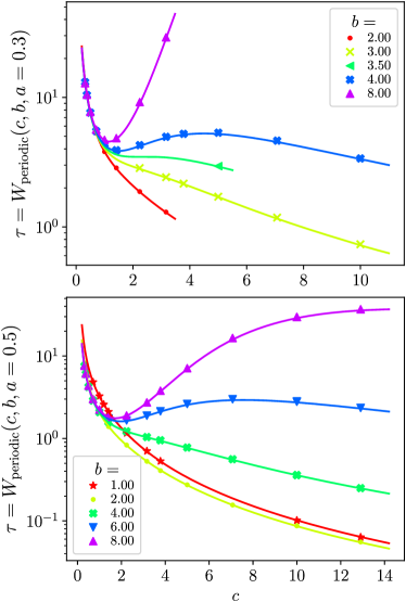
Figure 7: MFPT versus $c$ for the periodic resetting protocol in 2D for finite $b$ and $a=0.3$ (top panel) and $a=0.5$ (bottom panel). Continuous lines are the the theoretical predictions of Eq. 112 and the symbols corresponds to the results obtained from the numerical integration of the Langevin equation. In the bottom panel ($a=0.5$), the curves for $b=6$ and $b=4$ illustrate the two different regimes, whereas the phase transition appears at lower $b$ for $a=0.3$ (top pannel).

The comparison with the numerical simulation obtained from the numerical integration of the Langevin dynamics is plotted in Fig. (7) for two different $a$ and various $b$’s. The agreement is excellent and the presence of a metastable minimum for $b>b_{c}$ and a monotonous decrease for smaller $b$ confirm the presence of the dynamical phase transition in 2D for the periodic resetting. First passage times distributions has been numerically evaluated and the results at $c=2.23$, $a=0.75$ and various $b$’s are plotted in Fig. (8). Notice the presence of the spikes of period $T$ as was already observed in 1D.

Figure 8: Distributions of first passage times $t_{\text{f}}$ obtained from numerical simulations of the Langevin dynamics wih periodic reset at $c=2.23$, $a=0.75$ and various $b$’s.

IV.1.2 Experimental results

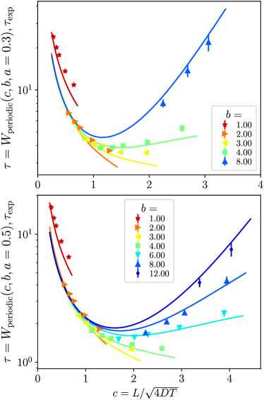
Figure 9: Experiment. $\tau$ versus $c$ for the periodic resetting protocol in 2D for finite $b$ and $a=0.3$ (top panel) and $a=0.5$ (bottom panel). Continuous lines are the the theoretical predictions of Eq. 112 with $\sigma=\sigma_{x,\text{exp}}$ and the symbols corresponds to the results obtained from the experimental data.

Testing experimentally the theoretical predictions of the MFPT in 2D presents two main chalenges. The first is that a very good statistics is needed to get results with a rather good accuracy for several values of $a,b$ and $c$. The second is due to the unavoidable asymmetries in the $x$ and $y$ direction especially on the variances of the initial position, due to laser beam anisotropy ($\sigma_{x,\text{exp}}/\sigma_{y,\text{exp}}=0.82$). In order to compare with the theory (which has not been extended to anisotropic initial distributions), we must choose a representative $\sigma$. We could define $\sigma_{\text{mean}}=\sqrt{\smash{(\sigma_{x,\text{exp}}^{2}+\sigma_{y,\text{exp}}^{2})}/2}=$38\text{\,}\mathrm{nm}$$. However, this does not do justice to the fact that when the target is on the $x$ axis, a larger $\sigma_{x}$ decreases the MFPT, while a larger $\sigma_{y}$ increases the MFPT. Thus, $\sigma=\sigma_{x,\text{exp}}=$34\text{\,}\mathrm{nm}$$ is a better choice to compare with the theory. The results are reported in Fig. (9) where we observe a rather good agreement with the theoretical predictions in spite of the approximated $\sigma$ and the rather low statistics (about $10^{4}$ trajectories). The same results are reported against $\sigma_{\text{mean}}$ in Fig. (17), and the effect of anisotropy is discussed in annex F. While it is important ($\sim$10% error on $\tau$), it is not enough to explain the mismatch. Again, the fact that the difference is significant only for low MFPTs and high $c$ indicates that it may come from the limited experimental acquisition rate.

IV.2 Poissonian resetting in 2 dimensions

Figure 10: MFPT versus $c$ for the Poissonian resetting protocol in 2D for $b\rightarrow\infty$ and several values of $a$. Continuous lines are the the theoretical predictions of Eq. 89 and the symbols corresponds to the results obtained from the numerical integration of the Langvin equation.

Figure 11: $\tau$ versus $c$ for the Poissonian resetting protocol in 2D for finite $b$ and $a=0.25$ (top panel) and $a=0.5$ (bottom panel). Continuous lines are the the theoretical predictions of Eq. 85 and the symbols corresponds to the results obtained from the numerical integration of the Langvin equation. In the bottom panel, curves for $b=6$ and $b=4$ illustrate the two different regimes.

We discuss here the results with the Poissonian resetting. In this case the 2D MFPT can be analytically computed explicitly (see Eqs. 85 and 89 in Appendix E). Our experimental data statistics is to low to compare the theoretical 2D MFPT with experimental results for the Poissonian resetting protocol. Indeed in that case one needs higher statistics to sample correctly the exponential distribution of free diffusion times and then have a good estimate of the MFPT for the three parameters $(a,b,c)$. We thus compare the analytical results with a numerical integration of the Langevin equation for different values of $b$ and $a$. The numerical results for $b\rightarrow\infty$ (i.e. $\sigma\rightarrow 0$) are compared in Fig. (10) with theoretical prediction (Eq. 89) for several values of $a$. The theoretical predictions at finite $b$ are compared with the numerical results in Fig. (11) for two values of $a$. The agreement is very good and one can notice that, as in the 1D case, the presence of a metastable minimum (e.g. see $b=6$).

This demonstrates that, as in 1D, the 2D MFPT curve always features a metastable minimum for higher values of $b$, and a dynamical phase transition for closer targets.

V Discussion and conclusions

We have studied theoretically, numerically and experimentally, in one and two dimensions, the statistics of first-passage times to a target by a Brownian particle subjected to two different resetting protcols: (i) periodic resetting with period $T$ and (ii) Poissonian resetting with a constant $r$. In both cases, the distribution of the initial/reset position is not a delta function, but has a Gaussian distribution with a finite width $\sigma$, corresponding to the equilibrium Gibbs-Boltzmann position distribution of the particle in a harmonic trapping potential. We have shown that the presence of a finite width $\sigma$ in the resetting position has a profound and interesting effect on the statistics of first-passage times. We have shown that, both in 1 and 2 dimensions and in both protocols, the curve of the rescaled mean first-passage time $\tau$ as a function of the parameter $c=L/\sqrt{4DT}$ for periodic protocol (and $c=\sqrt{r/D}\,L$ for Poissonian protocol) has very different behavior for $b=L/\sigma>b_{c}$ and $b<b_{c}$. For $b>b_{c}$, the MFPT curve has two minima, one at a finite value $c_{1}(b)$ and the other at $c\to\infty$, separated by a maximum at $c=c_{2}(b)$. The first minimum turns out to be metastable and it disappears for $b<b_{c}$ where the MFPT curve decreases monotonbically with increasing $c$. We have argued that this phase transition at $b=b_{c}$ is dynamical in the sense that it occurs when two different time scales $T_{1}\sim\mathcal{O}(L^{2}/D)$ and $T_{2}\sim\mathcal{O}(\sigma^{2}/D)$ merge with each other.

We find the existence of the metastable minimum in MFPT for $b>b_{c}$ and the subsequent disappearence of it (when $b$ redcues below $b_{c}$) via a dynamical phase transition, rather robust. It exists in both 1D and 2D and for two different types of resetting protocols. For the periodic protocol, we also computed and measured the full PDF of the first-passage times and found that it displays striking spikes after each resetting event, a clear effect of the finiteness of the variance of the initial position. Both in one and two dimensions the numerical and experimental data agree well with theoretical predictions, but the experiment is not a mere test of the theory. Indeed, taking into account the experimental finite width $\sigma$ of optical trap resetting shed light on the dynamical phase transtion described here. We also detailed experimental difficulties encountered in first passage experiments. When the particle is free for a very long time (small $c$), one has to tackle with sedimentation or particle loss. On the very short times (large $c$), we have shown that finite sampling time affects the results, because some first-passages are not detected, leading to an overestimation of the first-passage time. In 2 dimensions the anisotropy of the optical trap and statistics limit the accuracy. Finally, it would be interesting to extend this work by taking into account the role of hydrodynamic memory effects and particle inertia in future theoretical developments and to compare with very fast sampling rate experiments.

Appendix A Preliminaries

In this Appendix and in Appendices B and C we summarize, for the 1D case, how the theoretical predictions plotted in Figs. 2), 3) and 4) of the main text have been obtained, both for periodic and random resetting protocols. Much of these 1D results can be found in Supplemental Material of Besga et al. (2020), but we prefer to recall them here to have a full description of the resetting protocol in 1D and 2D. The theoretical results for 2D are entirely new and are presented in Appendices D and E respectively.

As already pointed out in the main text we consider here a realistic situation in which the initial position at the begining of each free diffusion period (between successive resetting events) has a Gaussian distribution of width $\sigma$. The mean first-passage time (MFPT), in the presence of resetting for either of the two protocols, was previously computed only for the restting to a fixed initial position $x_{0}$ Evans and Majumdar (2011a, b); Pal et al. (2016); Bhat et al. (2016); Evans et al. (2020). In practice this is not possible to realize experimentally because of the finite stiffness $\kappa$ of the trap which resets the particle to the initial position. In an optical trap at temperature $T$, the resetting position is always Gaussian distributed with a finite variance $\sigma^{2}=k_{B}T/\kappa$ given by equipartition. As $\kappa$ is proportional to the laser intensity starting with $\sigma=0$ would imply to trap with an infinite power which is of course not possible. Thus we study here the influence of a finite nonzero $\sigma$ on MFPT.

Consider a searcher undergoing a generic stochastic dynamics starting, say, at the initial position $x_{0}$. The immobile target is located at $x=L$. To compute the MFPT of a generic stochastic process, it is most convenient to first compute the survival probability or persistence Majumdar (1999); Redner (2001); Majumdar (2010); Bray et al. (2013) $S(t|x_{0})$, starting from $x_{0}$. This is simply the probability that the searcher, starting its dynamics at $x_{0}$ at $t=0$, does not find the target up to time $t$. The first-passage probability density $F(t|x_{0})$ denotes the probability density to find the target for the first time at $t$. The two quantities $F(t|x_{0})$ and $S(t|x_{0})$ are simply related to each other via $S(t|x_{0})=\int_{t}^{\infty}F(t^{\prime}|x_{0})\,d{t^{\prime}}$, because if the target is not found up to $t$, the first-passage time must occur after $t$. Taking a derivative with respect to $t$ gives

$$F(t|x_{0})=-\derivative{S(t|x_{0})}{t}\,.$$ (9)

Hence, if we can compute $S(t|x_{0})$ (which is often easier to compute), we obtain $F(t|x_{0})$ simply from Eq. (9). Once we know $F(t|x_{0})$, the MFPT is just its first moment

$$\langle t_{f}\rangle(x_{0})=\int_{0}^{\infty}t\,F(t|x_{0})\differential{t}=\int_{0}^{\infty}S(t|x_{0})\differential{t}\,,$$ (10)

where in arriving at the last equality, we substituted Eq. (9) and did integration by parts. Below, we will first compute the survival probability $S(t|x_{0})$ for fixed $x_{0}$ and then average over the distribution of $x_{0}$. We will consider the two protocols separately.

Appendix B Protocol-1: Periodic Resetting to a random initial position

We consider an overdamped diffusing particle that starts at an initial position $x_{0}$, which is drawn from a distribution ${\cal P}(x_{0})$. The particle diffuses for a fixed period $T$ and then its position is instantaneously reset to a new position $z$, also drawn from the same distribution ${\cal P}(z)$. Then the particle diffuses again for a period $T$, followed by a reset to a new position $z^{\prime}$ drawn from ${\cal P}(z)$ and the process continues. We assume that after each resetting, the reset position $z$ is drawn independently from cycle to cyle from the same distribution ${\cal P}(z)$. We also have a fixed target at a location $L$. For fixed $L$, $T$ and ${\cal P}(z)$, We want to first compute the mean first-passage time $\langle t_{f}\rangle$ to find the target and then optimize (minimize) this quantity with respect to $T$ (for fixed $L$ and ${\cal P}(z)$). We first compute the MFPT for arbitrary ${\cal P}(z)$ and then focus on the experimentally relevant Gaussian case.

We first recall that for a free diffusing particle, starting at an initial position $x_{0}$, the survival probability that it stays below the level $L$ up to time $t$ is given by Majumdar (1999); Redner (2001); Majumdar (2010); Bray et al. (2013)

$$S(t|x_{0})=\erf\left(\frac{|L-x_{0}|}{\sqrt{4Dt}}\right)\,,$$ (11)

where $\erf(z)=(2/\sqrt{\pi})\,\int_{0}^{z}e^{-u^{2}}\differential{u}$ is the error function and $D$ is the diffusion constant. If the initial position is chosen from a distribution ${\cal P}(x_{0})$, then the survival probability, averaged over the initial position, is given by

$$Q_{1}(t)=\int_{-\infty}^{\infty}\differential{x_{0}}{\cal P}(x_{0})\,S(t|x_{0})=\int_{-\infty}^{\infty}\differential{x_{0}}{\cal P}(x_{0})\,{\rm erf}\left(\frac{|L-x_{0}|}{\sqrt{4Dt}}\right)\,.$$ (12)

Now, consider our protocol. Let us compute the survival probability $Q(t)$ up to time $t$, averaged over the distribution of the starting position at the begining of each cycle. Then it is easy to see the following.

• $0<t\leq T$: If the measurement time $t$ lies in the first cycle of diffusion, then the survival probability upto time $t$ is simply $Q_{1}(t)$ given in Eq. (12), since no resetting has taken place up to $t$ yet. Note that at the end of the period $[0,T]$, the survival probability is simply $Q_{1}(T)$.

• $T<t\leq 2T$: In this case, the particle has to first survive the period $[0,T]$ with free diffusion: this occurs with probability $Q_{1}(T)$. Then from time $T$ till $T<t\leq 2T$, it also undergoes a free diffusion but starting from a new reset position $z$ drawn from ${\cal P}(z)$. Hence, the survival probability up to $T<t\leq 2T$ is given by the product of these two events

  $$Q_{2}(t)=Q_{1}(T)\,\int_{-\infty}^{\infty}\differential{z}{\cal P}(z)\,{\rm erf}\left(\frac{|L-z|}{\sqrt{4D(t-T)}}\right)\,.$$ (13)

  Note that at the end of the cycle

  $$Q_{2}(2T)=Q_{1}^{2}(T)$$ (14)

  where $Q_{1}(T)$ is given by Eq. (12).

• $2T<t\leq 3T$: By repeating the above argument

  $$Q_{3}(t)=Q_{1}(2T)\,\int_{-\infty}^{\infty}\differential{z}{\cal P}(z)\,{\rm erf}\left(\frac{|L-z|}{\sqrt{4D(t-2T)}}\right)=Q_{1}^{2}(T)\,\int_{-\infty}^{\infty}\differential{z}{\cal P}(z)\,{\rm erf}\left(\frac{|L-z|}{\sqrt{4D(t-2T)}}\right)$$ (15)

  At the end of the 3rd cycle

  $$Q_{3}(3T)=Q_{1}^{3}(T)$$ (16)

  where $Q_{1}(T)$ is given by Eq. (12).

• $(n-1)T<t\leq n\,T$: For the $n$-th cycle, we have then

  $$Q_{n}(t)=\left[Q_{1}(T)\right]^{n-1}\,\int_{-\infty}^{\infty}\differential{z}{\cal P}(z)\,{\rm erf}\left(\frac{|L-z|}{\sqrt{4D(t-(n-1)\,T)}}\right)$$ (17)

Hence, the survival probability $Q(t)$ is just $Q_{n}(t)$ if $t$ belongs to the $n$-th period, i.e., if $(n-1)T<t\leq n\,T$, where $n=1,\,2,\,\ldots$. In other words, for fixed $t$, we need to find the cycle number $n$ associated to $t$ and then use the formula for $Q_{n}(t)$ in (17). Mathematically speaking

$$Q(t)=\sum_{n=1}^{\infty}Q_{n}(t)\,\operatorname{I}_{(n-1)T<t\leq n\,T}$$ (18)

where the indicator function $\operatorname{I}_{A}=1$ if the clause $A$ in the subscript is satisfied and is zero otherwise.

The mean first-passage time $\langle t_{f}\rangle$ to location $L$, average over the distribution of $x_{0}$, is then given from Eq. (10) as

$$\langle t_{f}\rangle=\int_{0}^{\infty}\differential{t}Q(t)$$ (19)

where $Q(t)$ is the survival probability up to time $t$ in (18). Using the results above for different cycles, we can evaluate this integral in Eq. (19) by dividing the time integral over different cycles. This gives

$$\langle t_{f}\rangle=\sum_{n=1}^{\infty}\int_{(n-1)T}^{nT}\differential{t}Q_{n}(t) = \sum_{n=1}^{\infty}\left[Q_{1}(T)\right]^{n-1}\,\int_{(n-1)T}^{nT}\differential{t}\int_{-\infty}^{\infty}\differential{z}{\cal P}(z)\,\erf\left(\frac{|L-z|}{\sqrt{4D(t-(n-1)\,T)}}\right)$$ (20)

$$= \sum_{n=1}^{\infty}\left[Q_{1}(T)\right]^{n-1}\,\int_{0}^{T}\differential{\Delta}\int_{-\infty}^{\infty}\differential{z}{\cal P}(z)\,\erf\left(\frac{|L-z|}{\sqrt{4D\,\Delta}}\right)\,,$$

where in the last line we made a change of variable $\tau=t-(n-1)T$. The sum on the right hand side (rhs) of Eq. (20) can be easily performed as a geometric series. This gives

$$\langle t_{f}\rangle=\frac{\int_{0}^{T}\differential{\tau}\int_{-\infty}^{\infty}\differential{z}{\cal P}(z)\,\erf\left(\frac{|L-z|}{\sqrt{4D\,\tau}}\right)}{1-Q_{1}(T)}\,.$$ (21)

The denominator can be further simplified as

$$1-Q_{1}(T)=1-\int_{-\infty}^{\infty}\differential{z}{\cal P}(z)\,{\rm erf}\left(\frac{|L-z|}{\sqrt{4DT}}\right)=\int_{-\infty}^{\infty}\differential{z}{\cal P}(z)\,{\rm erfc}\left(\frac{|L-z|}{\sqrt{4DT}}\right)$$ (22)

where $\operatorname{erfc}(z)=1-\erf(z)=(2/\sqrt{\pi})\int_{z}^{\infty}e^{-u^{2}}\differential{u}$ denotes the complementary error function. Note that we have used the normalization: $\int_{-\infty}^{\infty}{\cal P}(z)\differential{z}=1$. Substituting the result of Eq. (22) in Eq. (21) we get our final formula, valid for arbitrary reset/initial distribution ${\cal P}(z)$

$$\langle t_{f}\rangle=\frac{\int_{0}^{T}\differential{\tau}\int_{-\infty}^{\infty}\differential{z}{\cal P}(z)\,\erf\left(\frac{|L-z|}{\sqrt{4D\,\tau}}\right)}{\int_{-\infty}^{\infty}\differential{z}{\cal P}(z)\,\operatorname{erfc}\left(\frac{|L-z|}{\sqrt{4DT}}\right)}\,.$$ (23)

The full first-passage probability density $F(t)$, averaged over the distribution of $x_{0}$, is then given by

$$F(t)=-\derivative{Q}{t}\,,$$ (24)

where $Q(t)$ is given in Eq. (18).

B.1 Reset to a Gaussian initial distribution

As an example, let us consider the Gaussian distribution for the reset/initial position

$${\cal P}(x_{0})=\frac{1}{\sqrt{2\,\pi\,\sigma^{2}}}\,e^{-{x_{0}}^{2}/{2\sigma^{2}}}$$ (25)

where $\sigma$ denotes the width. In this case, the survival probability $Q_{1}(T)$ at the end of the first cycle, is given from Eq. (12) upon setting $t=T$

$$Q_{1}(T)=\int_{-\infty}^{\infty}\frac{\differential{x_{0}}}{\sigma\,\sqrt{2\pi}}\,e^{-{x_{0}}^{2}/{2\sigma^{2}}}\,\erf\left(\frac{L-x_{0}}{\sqrt{4\,D\,T}}\right)\,.$$ (26)

Let us introduce two dimensionless constants $b$ and $c$

$$b=\frac{L}{\sigma}\,;\quad\quad\quad\quad c=\frac{L}{\sqrt{4DT}}\,.$$ (27)

Then in terms of these two constants, Eq. (26), after suitable rescaling, can be simplified to

$$Q_{1}(T)=\frac{b}{\sqrt{2\pi}}\,\int_{-\infty}^{\infty}\differential{y}e^{-b^{2}\,y^{2}/2}\,\erf\left(c\,|1-y|\right)\,.$$ (28)

Note that in the limit of $b\to\infty$, i.e., when $L\ll\sigma$ (corresponding to resetting to the origin) one gets

$$Q_{1}(T)\Big{|}_{b\to\infty}=\erf(c)\,,$$ (29)

where we used $(b/\sqrt{2\pi})\,e^{-b^{2}\,y^{2}/2}\to\delta(y)$ when $b\to\infty$.

B.1.1 Mean first-passage time

Substituting the Gaussian ${\cal P}(z)$ in Eq. (23), and rescaling $\tau=v\,T$ we can write everything in dimensionless form

$$\tau=\frac{4D\langle t_{f}\rangle}{L^{2}}=\frac{\int_{0}^{1}\differential{v}\int_{-\infty}^{\infty}\differential{u}e^{-u^{2}/2}\,{\rm erf}\left(\frac{c}{\sqrt{v}}\,|1-u/b|\right)}{c^{2}\,\int_{-\infty}^{\infty}\differential{u}e^{-u^{2}/2}\,\operatorname{erfc}\left(c\,|1-u/b|\right)}\,\equiv w(b,c)$$ (30)

where the dimensionless constants $b$ and $c$ are given in Eq. (27). It is hard to obtain a more explicit expression for the function $w(b,c)$ in Eq. (30). But it can be easily evaluated numerically.

To make further analytical progress, we first consider the limit $\sigma\to 0$, i.e., $b=L/\sigma\to\infty$. In this limit, the reset distribution ${\cal P}(z)\to\delta(z)$. Hence, Eq. (23) or equivalently Eq. (30) simplifies considerably and the integrals can be evaluated explicitly. We obtain an exact expression

$$\tau=\frac{4D\langle t_{f}\rangle}{L^{2}}=\frac{{\rm erf}(c)+2c\left(e^{-c^{2}}/\sqrt{\pi}-c\,\operatorname{erfc}(c)\right)}{c^{2}\,\operatorname{erfc}(c)}\equiv w(b\to\infty,c)\equiv w(c)$$ (31)

where we recall $c=L/\sqrt{4DT}$. In Fig. 2 of the main text, we plot the function $w(c)$ vs. c, which has a minimum at

$$c_{\rm opt}=0.738412...$$ (32)

At this optimal value, $\tau_{\rm opt}=w(c_{\rm opt})=5.34354\ldots$. Hence, the optimal mean first-passage time to find the target located at $L$ is given by

$$\langle t_{f}\rangle_{\rm opt}=(5.34354\ldots)\,\frac{L^{2}}{4D}\,.$$ (33)

Note that this result is true in the limit $b=L/\sigma\to\infty$, i.e., when the target is very far away from the starting/resetting position. In this limit, our result coincides with Ref. Pal et al. (2016) where the authors studied periodic resetting to the fixed initial position $x_{0}=0$ by a different method. This is expected since the limit $b=L/\sigma\to\infty$ limit is equivalent to $\sigma\to 0$ (with fixed $L$) and one would expect to recover the fixed initial position results.

But the most interesting and unexpected result occurs for finite $b$. In this case we can evaluate the rhs of Eq. (30) numerically. This has been done to plot the continuous lines in Fig. 3 of the main text, which shows the existence of a metastable minimum for $b>b_{c}\simeq 2.3$

B.1.2 Full first-passage probability density $F(t)$

The first-passage probability density can be computed from Eq. (24) and is plotted in Fig. 2 of the main text. For a finite $b=L/\sigma$ we see those spectacular spikes at the beginning of each cycle. In this subsection, we analyse the origin of these spikes. For this let us analyse the survival probability $Q_{n}(t)$ in Eq. (17) close to the epoch $n\,T$, i.e., when the $n$-th period ends. We set $t=n\,T+\Delta$ where $\Delta$ is small. For $\Delta>0$, we are in the $(n+1)$-th cycle, while for $\Delta<0$ we are in the $n$-th cycle. We consider the $\Delta>0$ and $\Delta<0$ cases separately.

The case $\Delta>0$: Since $t=n\,T+\Delta$ with $\Delta>0$ small, $t$ now belongs to the $(n+1)$-th cycle, so we replace $n$ by $n+1$ in Eq. (17) and get

$$Q_{n+1}(t=n\,T+\Delta)=\left[Q_{1}(T)\right]^{n}\,\int_{-\infty}^{\infty}\frac{\differential{z}}{\sigma\,\sqrt{2\pi}}\,e^{-z^{2}/{2\sigma^{2}}}\,\erf\left(\frac{|L-z|}{\sqrt{4\,D\,\Delta}}\right)\,,$$ (34)

where $Q_{1}(T)$ is given in Eq. (28). It is convenient first to use the relation $\erf(z)=1-\operatorname{erfc}(z)$ and rewrite this as

$$Q_{n+1}(t=n\,T+\Delta)=\left[Q_{1}(T)\right]^{n}\,\left[1-\int_{-\infty}^{\infty}\frac{\differential{z}}{\sigma\,\sqrt{2\,\pi}}\,e^{-z^{2}/{2\sigma^{2}}}\,\operatorname{erfc}\left(\frac{|L-z|}{\sqrt{4\,D\,\Delta}}\right)\,\right]\,$$ (35)

To derive the small $\Delta$ asymptotics, we make a change of variable $(L-z)/\sqrt{4\,D\,\Delta}=y$ on the rhs of Eq. (35). This leads to, using $b=L/\sigma$,

$$Q_{n+1}(t=n\,T+\Delta)=\left[Q_{1}(T)\right]^{n}\,\left[1-\frac{\sqrt{4\,D\,\Delta}}{L}\,\frac{b}{\sqrt{2\,\pi}}\,\int_{-\infty}^{\infty}\differential{y}e^{-\frac{b^{2}}{2}\,(1-\sqrt{4\,D\,\Delta}\,y/L)^{2}}\,\operatorname{erfc}(|y|)\,\right]\,.$$ (36)

We can now make the limit $\Delta\to 0$. To leading order in $\Delta$, we can set $\Delta=0$ inside the exponential in the integrand on the rhs and using $\int_{-\infty}^{\infty}\differential{y}\operatorname{erfc}(|y|)=2/\sqrt{\pi}$ we get

$$Q_{n+1}(t=n\,T+\Delta)\simeq\left[Q_{1}(T)\right]^{n}\,\left[1-A_{+}(b)\,\sqrt{\Delta}\,\right]\,,\quad\quad A_{+}(b)=\sqrt{\frac{8\,D}{\pi^{2}\,L^{2}}}\,b\,e^{-b^{2}/2}\,.$$ (37)

Taking derivative with respect to time, i.e., with respect $\Delta$, we find that as $\Delta\to 0^{+}$, the first-passage probability denity $F(t)=-dQ/dt$ diverges for any finite $b$ as

$$F(t=n\,T+\Delta)\simeq\frac{A_{n}(b)}{\sqrt{\Delta}}$$ (38)

where the amplitude $A_{n}(b)$ of the inverse square root divergence is given by the exact formula

$$A_{n}(b)=\sqrt{\frac{2D}{\pi^{2}\,L^{2}}}\,b\,e^{-b^{2}/2}\,\left[Q_{1}(T)\right]^{n}\,$$ (39)

where $Q_{1}(T)$ (which also depends on $b$) is given in Eq. (28). This inverse square root divergence at the begining of any cycle, for any finite b, describes the spikes in Fig. 2 of the main text. Note that the amplitude $A_{n}(b)$ of the $n$-th spike in Eq. (39) decreases exponentially with $n$, as seen also in Fig. 2 of the main text.

Interestingly, we see from Eq. (39) that the amplitudes of the spikes decrease extremely fast as $b$ increases and the spikes disappear in the $b\to\infty$ limit. Since $b=L/\sigma$, we see that the limit $b\to\infty$ corresponds to $\sigma\to 0$ limit (for fixed $L$). This is indeed the case where one resets always to the origin. In fact, if we first take the limit $b\to\infty$ keeping $\Delta$ fixed and then take the limit $\Delta\to 0$, we get a very different reesult. Taking $b\to\infty$ limit first in Eq. (36) we get,

$$Q_{n+1}(t=n\,T+\Delta)\Big{|}_{b\to\infty}=\left[Q_{1}(T)\right]^{n}\left[1-\operatorname{erfc}\left(\frac{L}{\sqrt{4\,D\,\Delta}}\right)\right]\,,$$ (40)

where $Q_{1}(T)$ now is given in Eq. (29). Taking a derivative with respect $t$, i.e., with respect to $\Delta$, we get the first-passage probability density

$$F(t=n\,T+\Delta)\Big{|}_{b\to\infty}=\left[Q_{1}(T)\right]^{n}\,\frac{L}{\sqrt{4\,\pi\,D\,\Delta^{3}}}\,e^{-L^{2}/(4\,D\,\Delta)}\,.$$ (41)

Thus, in the $b\to\infty$ limit, the first pasage probability actually vanishes extremely rapidly as $\Delta\to 0$ due to the essential singular term $\sim e^{-L^{2}/(4\,D\,\Delta)}$.

To summarize, the behavior of the first-passage probability density at the begining of the $n$-th period is strikingly different for $\sigma=0$ ($b\to\infty)$ and $\sigma>0$ ($b$ finite): in the former case it vanishes extremely rapidly as $t\to n\,T$ from above, while in the latter case it diverges as an inverse sqaure root leading to a spike at the begining of each period. Thus the occurrence of spikes for $\sigma>0$ is a very clear signature of the finiteness of $\sigma$. Physically, a spike occurs because if $\sigma$ is finite, immedaitely after each resetting the searcher may be very close to the target and has a finite probability of finding the target immediately without further diffusion.

The case $\Delta<0$: When $t=n\,T+\Delta$ with $\Delta<0$, the effects are not so prominent as in the $\Delta>0$ case. For $\Delta<0$, since $t$ belongs to the $n$-th branch, we consider the formula in Eq. (17) with $n$ and get

$$Q_{n}(t=n\,T+\Delta)=\left[Q_{1}(T)\right]^{n-1}\,\int_{-\infty}^{\infty}\frac{\differential{z}}{\sigma\,\sqrt{2\pi}}\,e^{-z^{2}/{2\sigma^{2}}}\,\erf\left(\frac{|L-z|}{\sqrt{4\,D\,(T+\Delta)}}\right)\,.$$ (42)

Now taking the $\Delta\to 0$ limit in Eq. (42) is straightforward since there is no singular behavior. Just Taylor expanding the error function for small $\Delta$ up to $O(\Delta)$, and making the change of variable $(L-z)/\sqrt{4\,D\,T}=y$, we obtain

$$Q_{n}(t=n\,T+\Delta)=\left[Q_{1}(T)\right]^{n}-\Delta\,B_{n}(b)+O(\Delta^{2})\,,$$ (43)

where the constant

$$B_{n}(b)=\frac{b\,\left[Q_{1}(T)\right]^{n-1}}{c\,T\,\pi\,\sqrt{2}}\,\int_{-\infty}^{\infty}\differential{y}|y|\,e^{-y^{2}}\,e^{-\frac{b^{2}}{2}\,(1-c\,y)^{2}}\,,$$ (44)

with $c=L/\sqrt{4\,D\,T}$. Taking derivative with respect to $\Delta$ in Eq. (43) gives the leading behavior of the first-passage probability density: it approaches a constant as $\Delta\to 0$

$$F(t=n\,T+\Delta)\simeq B_{n}(b)\,.$$ (45)

One can easily check that even in the $b\to\infty$ limit, this constant remains nonzero and is given by

$$F(t=n\,T+\Delta)\Big{|}_{b\to\infty}\simeq\frac{\left[Q_{1}(T)\right]^{n-1}}{\sqrt{\pi}\,T\,c^{3}}\,e^{-1/c^{2}}\,,$$ (46)

where $Q_{1}(T)$ is now given in Eq. (29). Thus, for any $\sigma\geq 0$, as one approaches the epoch $t=n\,T$ from the left, i.e., at the end of the $(n-1)$-th cycle, the first-passage probability density approaches a constant $B_{n}(b)$ given in Eq. (44). This constant remains finite even when $b\to\infty$. On this side, there is no spectacular effect distinguishing $\sigma=0$ ($b\to\infty$) and $\sigma>0$ (finite $b$), as is the case on the right side of the epoch $n\,T$. On the right, for finite $b$ we have an inverse square root divergence as in (38), while for $b\to\infty$, it vanishes rapidly as $\Delta\to 0$. Thus in the large $b$ limit, we have a discontuity or drop from left to right (not a spike) as we see in the inset of Fig. 2 in the main text.

Appendix C Protocol-2: Random resetting to a random initial position

We consider an overdamped diffusing particle that starts at an initial position $x_{0}$, which is drawn from a distribution ${\cal P}(x_{0})$. The particle diffuses for a random interval $T$ drawn from an exponential distribution $P(T)=r\,e^{-r\,T}$ and then its position is instantaneously reset to a new position $z$, also drawn from the same initial distribution ${\cal P}(z)$. Then the particle diffuses again for another random interval $T$ (again drawn from the exaponential distribution $P(T)$), followed by a reset to a new position $z^{\prime}$ drawn from ${\cal P}(z)$ and the process continues. We assume that after each resetting, the reset position $z$ is drawn independently from cycle to cyle from the same distribution ${\cal P}(z)$. Similarly, the interval $T$ is also drawn independently from cycle to cyle from the same distribution $P(T)=r\,e^{-r\,T}$. We also have a fixed target at a location $L$. For fixed $L$, $r$ and ${\cal P}(z)$, We want to first compute the mean first-passage time $\langle t_{f}\rangle$ to find the target and then optimize (minimize) this quantity with respect to $r$ (for fixed $L$ and ${\cal P}(z)$). Recall that in protocol-1, we just had a fixed $T$, but in protocol-2 $T$ is exponentially distributed.

In this case, the mean first-passage time $\langle t_{f}\rangle$ has a simple closed formula. This formula can be derived folllowing steps similar to those in Ref. Evans and Majumdar (2011b). Skipping further details, we find

$$\langle t_{f}\rangle=\frac{1}{r}\,\left[\frac{1}{\int_{-\infty}^{\infty}\differential{z}{\cal P}(z)\,\exp\left(-\sqrt{\frac{r}{D}}\,|L-z|\right)}-1\right]\,.$$ (47)

Consider the special case of Gaussian distribution of Eq. (25) Substituting this Gaussian ${\cal P}(z)$ in Eq. (47), and performing the integral explicitly, we get the dimensionless mean first-passage time

$$\tau=\frac{4D\langle t_{f}\rangle}{L^{2}}=\frac{4}{c^{2}}\,\left[\frac{2\,e^{-c^{2}/{2b^{2}}}}{e^{c}\,\operatorname{erfc}\left(\frac{1}{\sqrt{2}}\left(\frac{c}{b}+b\right)\right)+e^{-c}\,\operatorname{erfc}\left(\frac{1}{\sqrt{2}}\left(\frac{c}{b}-b\right)\right)}-1\right]\,\equiv w_{2}(b,c)$$ (48)

where the dimensionless constants $b$ and $c$ are given by

$$b=\frac{L}{\sigma}\,;\quad\quad\quad\quad c=\sqrt{\frac{r}{D}}\,L\,.$$ (49)

Recall that in periodic protocol (with a fixed $T$ discussed in section B.1) , the parameter $b=L/\sigma$ is the same, but the parameter $c=L/\sqrt{4DT}$ is different. In protocol-2, the reset rate $r$ effectively plays the role of $1/T$ in protocol-1.

The formula for $w_{2}(b,c)$ in Eq. (48) for protocol-2 is simpler and more explicit, compared to the equivalent formula Eq.30 for protocol-1.

In Eq. (48), consider first the limit $b\to\infty$, i.e., resetting to a fixed initial condition. In this case, Eq. (48) reduces precisely to the formula derived by Evans and Majumdar Evans and Majumdar (2011a)

$$\tau=w_{2}(b\to\infty,c)=\frac{4}{c^{2}}\,\left[e^{c}-1\right]\,.$$ (50)

In this $b\to\infty$ limit, $\tau$ as a function of $c$, has a unique minimum at $c=c^{*}=1.59362\ldots$, where $\tau(c=c^{*})=6.17655\ldots$.

For finite fixed $b$, it is very easy to plot the function $w_{2}(b,c)$ vs. $c$ given in Eq. (48) and one finds that as in protocol-1, $w_{2}(b,c)$ first decreases with increasing $c$, achieves a minimum at certain $c_{1}(b)$, then starts increasing again–becomes a maximum at $c_{2}(b)$ and finally decreases for large $c$ as $\sim 1/c$ (this asymptotics for large $c$ can be computed exactly from Eq. (48)). Note that the actual values of $c_{1}(b)$band $c_{2}(b)$ are of course different in the two protocols. Interestingly, this metastable optimum time at $c=c_{1}(b)$ disappears when $b$ becomes smaller than a critical value $b_{c}=2.53884$. For $b<b_{c}$, the function $w_{2}(b,c)$ decreases monotonically with increasing $c$. Hence, for $b<b_{c}$, the best solution is $c=\infty$ (i.e., repeated resetting). The curves plotted in Fig. 4 of the main text correspond to this theoretical prediction and they have been checked experimentally and numerically. This numerical test allows us to clearly state that the small disagreement at small $b$ and large $c$ of the experimental data with the theoretical predictions is due to the maximum sampling rate of our analog to digital converter which was not fast enough to detect very short MFPT.

Appendix D General Setting: the survival probability of a Brownian walker in arbitrary dimensions

We first consider the general problem of the first-passage probability of a Brownian particle to a fixed target in $d$-dimensions (without any resetting). Resetting will be incorporated later. Consider a Brownian searcher in $d$-dimensions, starting initially at the position ${\vec{r}}_{0}$. An immobile point target is located at ${\vec{R}}_{\rm tar}$ with a tolerance radius $R_{\rm tol}$ (see Fig. 6).

If the searcher comes within the distance $R_{\rm tol}$ from the target at ${\vec{R}}_{\rm tar}$, the target is detected. Let $S_{0}(t|{\vec{r}}_{0})$ denote the survival probability, i.e., the probability that the target is not detected up to time $t$, given that the searcher starts at the initial position ${\vec{r}}_{0}$. Note that $S_{0}(t|{\vec{r}}_{0})$ depends implicitly on ${\vec{R}}_{\rm tar}$ and $R_{\rm tol}$, but we do not write them explicitly for the simplicity of notations. The subscript $0$ is $S_{0}|(t|{\vec{r}}_{0})$ denotes the fact that we are considering the problem without resetting. Suppose now that the initial position is random and drawn from a normalised probability distribution ${\cal P}({\vec{r}}_{0})$. Then the survival probability $Q_{0}(t)$, averaged over this distribution of the starting point of the searcher, is simply given by

$$Q_{0}(t)=\int S_{0}(t|{\vec{r}}_{0})\,{\cal P}({\vec{r}}_{0})\,\differential{{\vec{r}}_{0}}\,.$$ (51)

For later purposes, let us also define the Laplace transform of $Q_{0}(t)$ with respect to $t$ as follows

$${\tilde{Q}}_{0}(s)=\int_{0}^{\infty}Q_{0}(t)\,\mathrm{e}^{-s\,t}\differential{t}\,.$$ (52)

Let us suppose that we know the survival probability $Q_{0}(t)$ without resetting explicitly. Then we show below that when we switch on the resetting, the survival probability in the presence of resetting can be computed in terms of $Q_{0}(t)$ quite generally both for (I) the Poissonian resetting and (II) the periodic resetting.

Poissonian resetting: In this case, we choose the initial position ${\vec{r}}_{0}$ of the searcher from the distribution ${\cal P}({\vec{r}}_{0})$ at $t=0$ and let the particle (searcher) diffuse for a random time $T$ distributed exponentially, $P(T)=r\,\mathrm{e}^{-r\,T}$ where $r\geq 0$ is the resetting rate. At the end of the random period $T$, we reset the position of the searcher, i.e., we choose afresh the initial position from the same distribution ${\cal P}({\vec{r}}_{0})$ and again let it diffuse for a random period $T$ drawn afresh from $P(T)=r\,\mathrm{e}^{-r\,T}$ and so on. Let $Q_{r}(t)$ denote the survival probability, i.e., the probability that the target is not detected up to time $t$. The subscript $r$ denotes the presence of a nonzero resetting rate $r$. Considering several possibilities up to time $t$: (i) there is no resetting in $[0,t]$ (ii) there is exactly one resetting in $[0,t]$ (iii) there are exactly two resettings in $[0,t]$ etc, we can express $Q_{r}(t)$ as a series

$$Q_{r}(t)=\mathrm{e}^{-r\,t}Q_{0}(t)+r\,\int_{0}^{\infty}\differential{t_{1}}\int_{0}^{\infty}\differential{t_{2}}\mathrm{e}^{-r\,t_{1}}Q_{0}(t_{1})\,\mathrm{e}^{-r\,t_{2}}Q_{0}(t_{2})\,\delta(t_{1}+t_{2}-t)+\ldots\,.$$ (53)

The first term denotes the event when there is no resetting in $[0,t]$ which occurs with probability $\mathrm{e}^{-r\,t}$ and the particle survives with probability $Q_{0}(t)$ during the time interval. The second term denotes the event that exactly one resetting happens at time $t_{1}$ in $[0,t]$: this means a resetting occurs at $t_{1}$ and then there is no setting in the remaining interval $t_{2}=t-t_{1}$: this happens with probability density $r\,\mathrm{e}^{-r\,t_{1}}\differential{t_{1}}\,\mathrm{e}^{-r\,t_{2}}\,\delta(t_{1}+t_{2}-t)$. In addition the particle has to survive in both intervals $[0,t_{1}]$ and $[t_{1},t]$ which occurs with probability $Q_{0}(t_{1})\,Q_{0}(t_{2})$ where $t_{2}=t-t_{1}$. We have used the renewal property that makes the intervals between resettings statistically independent. Similarly, one can work out the probability of two resettings in $[0,t]$ etc. This somewhat formidable looking series in (53) simplifies enormously in the Laplace space. We define the Laplace transform

$${\tilde{Q}}_{r}(s)=\int_{0}^{\infty}Q_{r}(t)\,\mathrm{e}^{-s\,t}\differential{t}$$ (54)

and we recall that the Laplace transform ${\tilde{Q}}_{0}(s)$ is defined in (52). Taking Laplace transform of (53) with respect to $t$ one obtains

$${\tilde{Q}}_{r}(s)={\tilde{Q}}_{0}(r+s)+r\,\left[{\tilde{Q}}_{0}(r+s)\right]^{2}+r^{2}\,\left[{\tilde{Q}}_{0}(r+s)\right]^{3}+\ldots=\frac{{\tilde{Q}}_{0}(r+s)}{1-r\,{\tilde{Q}}_{0}(r+s)}\,,$$ (55)

The first-passage probability density $F_{r}(t)$, in the presence of the resetting, is given by

$$F_{r}(t)=-\derivative{Q_{r}(t)}{t}\,.$$ (56)

Consequently, its Laplace transform, using (56) and (55), is simply

$${\tilde{F}_{r}}(s)=\int_{0}^{\infty}F_{r}(t)\,\mathrm{e}^{-s\,t}\differential{t}=1-s\,{\tilde{Q}}_{r}(s)=\frac{1-(r+s)\,{\tilde{Q}}_{0}(r+s)}{1-r\,{\tilde{Q}}_{0}(r+s)}\,$$ (57)

where ${\tilde{Q}}_{0}(s)$ is the Laplace transform of the survival probability without resetting defined in (52). Finally, the mean first-passage time (MFPT), using the relation in (56), is given by

$$\langle t_{f}\rangle=\int_{0}^{\infty}t\,F_{r}(t)\differential{t}=\int_{0}^{\infty}Q_{r}(t)\differential{t}={\tilde{Q}}_{r}(s=0)=\frac{{\tilde{Q}}_{0}(r)}{1-r\,{\tilde{Q}}_{0}(r)}$$ (58)

where we used (55) in arriving at the last result. Thus, to summarize, in the presence of the Possonian resetting with rate $r$, we can in principle compute both $\langle t_{f}\rangle$ as well as the full distribution $F_{r}(t)$ (rather its Laplace transform), provided we know ${\tilde{Q}}_{0}(s)$, i.e., the Laplace transform of the survival probability $Q_{0}(t)$ without resetting.

Periodic resetting: As in the case of the Poissonian resetting, we choose the initial position ${\vec{r}}_{0}$ of the searcher from the distribution ${\cal P}({\vec{r}}_{0})$ at $t=0$ and let the particle (searcher) diffuse for a fixed period $T$. At the end of the period $T$, we reset the position of the searcher, i.e., we choose afresh the initial position from the same distribution ${\cal P}({\vec{r}}_{0})$ and again let it diffuse for a period $T$ and so on. We then ask: what is the survival probability $Q(t|T)$ that the target is not detected up to time $t$? Clearly if the measurement time $t$ belongs to the $n$-th period, i.e., $(n-1)T<t\leq n\,T$ (with $n=1,2,\ldots$) then the survival probability is given by

$$Q(t|T)=\left[Q_{0}(T)\right]^{n-1}\,Q_{0}\left(t-(n-1)T\right)\,;\quad{\rm for}\,\,\quad(n-1)T<t\leq n\,T$$ (59)

where $Q_{0}(t)$ is defined in (51). The formula (59) is easy to derive: (i) the target has to survive being detected for the full $(n-1)$ cycles prior to the running one at $t$ and (ii) in the running period since the time passed is $t-(n-1)T$ since the begining of the period, its survival probability is $Q_{0}\left(t-(n-1)T\right)$. Since the cycles are independent, the total survival probability is just the product over different periods till time $t$. Hence, for arbitrary $t$, we can write the survival probability as

$$Q(t|T)=\sum_{n=1}^{\infty}\left[Q_{0}(T)\right]^{n-1}\,Q_{0}\left(t-(n-1)T\right)\,\operatorname{I}_{(n-1)T<t\leq n\,T}$$ (60)

where the indicator function $\operatorname{I}_{A}=1$ if the clause $A$ in the subscript is satisfied and is zero otherwise. The first-passage probability density $F(t|T)$ (given the period of resetting $T$) is then given by

$$F(t|T)=-\derivative{Q(t|T)}{t}\,,$$ (61)

where $Q(t|T)$ is given in Eq. (60). The MFPT is given by the first moment of $F(t|T)$

$$\langle t_{f}\rangle=\int_{0}^{\infty}t\,F(t|T)\differential{t}=\int_{0}^{\infty}Q(t|T)\differential{t}$$ (62)

where we used (61) and integrated by parts using $Q(\infty|T)=0$. Plugging in the formula in (60) and integrating we get

$$\langle t_{f}\rangle=\sum_{n=1}^{\infty}\left[Q_{0}(T)\right]^{n-1}\int_{0}^{T}Q_{0}(\tau)\differential{\tau}=\frac{\int_{0}^{T}Q_{0}(t)\differential{t}}{1-Q_{0}(T)}\,,$$ (63)

where we recall that $Q_{0}(t)$ is the survival probability without resetting as defined in (51). Thus, as in the case of the Poissonian resetting, for periodic resetting with a period $T$ also, we can compute the MFPT $\langle t_{f}\rangle$ and the full first-passage time distribution $F(t|T)$, provided we know the survival probability $Q_{0}(t)$ without resetting.

Hence, to summarize, the central quantity of interest is the survival probability $Q_{0}(t)$ without resetting. If we know this object, then we can compute, in principle, the first-passage properties in the presence of resetting, both for the Poissonian as well as for the periodic protocol. Below, we will focus in $d=2$ (where experimental data is available) and first compute the survival probability $Q_{0}(t)$ without resetting, and then apply the general results above to compute the MFPT as well as the distribution of first-passage times for the two protocols. It turns out that the final formulae are a bit more explicit in the case of Poissonian resetting than the periodic resetting.

Appendix E Two dimensions

We want to first compute the survival probability $Q_{0}(t)$ without resetting, defined in (51), in dimension $d=2$. For this we need to first compute the survival probability $S_{0}(t|{\vec{r}}_{0})$, i.e., the probability that the Brownian searcher, starting at the fixed initial position ${\vec{r}}_{0}$, does not enter the circle of tolerance (of radius $R_{\rm tol}$) around the target located at ${\vec{R}}_{\rm tar}$ up to time $t$ (see Fig. 6). The result for $S_{0}(t|{\vec{r}}_{0})$ is actually well known Barzykin and Tachiya (1993); Blythe and Bray (2003); Evans and Majumdar (2014) and can be easily computed as follows. We first make a change of variable $\vec{r_{p}}=\vec{r}_{0}-{\vec{R}}_{\rm tar}$ so that the distance is measured with respect to the target center and we denote, for the simplicity of notations, $S_{0}(t|{\vec{r}}_{0})=S_{0}(t|\vec{r}_{p}+{\vec{R}}_{\rm tar})$ by $S(\vec{r}_{p},t)$. The subscript $p$ in $\vec{r_{p}}$ simply stands for ‘particle’.

Then $S(\vec{r}_{p},t)$ satisfies the diffusion equation

$$\partial_{t}S(\vec{r}_{p},t)=D\,\nabla_{\vec{r}_{p}}^{2}S(\vec{r}_{p},t)\,$$ (64)

in the region $r_{p}=|\vec{r}_{p}|>R_{\rm tol}$, with the absorbing boundary condition $S(r_{p}=R_{\rm tol},t)=0$. Using spherical symmetry, $S(\vec{r}_{p},t)$ depends only on $r_{p}=|\vec{r}_{p}|$ and hence (64) reduces to a one dimensional partial differential equation in the radial coordinate

$$\partial_{t}S(r_{p},t)=D\left[\partial_{r_{p}}^{2}S+\frac{2}{r_{p}}\,\partial_{r_{p}}S\right]\,;\quad{\rm for}\quad r_{p}>R_{\rm tol}\,.$$ (65)

with the boundary condition $S(r_{p}=R_{\rm tol},t)=0$ and also $S(r_{p}\to\infty,t)=1$. The latter condition follows from the fact that the particle must survive with probability $1$ up to a finite time $t$, if it starts infinitely far away from the target. The initial condition is $S(r_{p},0)=1$ for all $r_{p}>R_{\rm tol}$. To solve this partial differential equation, it is first convenient to take the Laplace transform with respect to $t$ and define ${\tilde{S}}(r_{p},s)=\int_{0}^{\infty}S(r_{p},t)\,\mathrm{e}^{-s\,t}\differential{t}$. Taking Laplace transform of (65) and using the initial condition, we arrive at an ordinary second order differential equation

$$D\,\left[\derivative[2]{\tilde{S}}{r_{p}}+\frac{2}{r_{p}}\,\derivative{\tilde{S}}{r_{p}}\right]=-1+s\,{\tilde{S}}\,$$ (66)

valid for $r_{p}>R_{\rm tol}$ with the boundary conditions: (i) ${\tilde{S}}(r_{p}=R_{\rm tol},s)=0$ and (ii) ${\tilde{S}}(r_{p}\to\infty,s)=1/s$. The latter condition follows from the boundary condition $S(r_{p}\to\infty,t)=1$. The inhomogeneous term on the right hand side of (66) can be eliminated by a shift ${\tilde{S}}(r_{p},s)\to{\tilde{S}}(r_{p},s)+1/s$. The solution of the resulting ordinary homogeneous differential equation is given by the limear combination of modified Bessel functions. Finally, retaining only the solution that satisfies the correct boundary conditions, one arrives at Barzykin and Tachiya (1993); Blythe and Bray (2003); Evans and Majumdar (2014)

$${\tilde{S}}(r_{p},s)=\frac{1}{s}\,\left[1-\frac{K_{0}\left(\sqrt{\frac{s}{D}}\,r_{p}\right)}{K_{0}\left(\sqrt{\frac{s}{D}}\,R_{\rm tol}\right)}\right]\,;\quad{\rm for}\,\,r_{p}\geq R_{\rm tol}\,$$ (67)

where $K_{\nu}(x)$ is the modified Bessel function of the second kind with index $\nu$ Gradshteyn and Ryzhik (1965). Translating back to the original coordinate and using $S_{0}(t|{\vec{r}}_{0})=S(r_{p}=|\vec{r}_{0}-\vec{R}_{\rm tar}|,\,t)$ we then have the exact solution in the Laplace space

$$\int_{0}^{\infty}S_{0}(t|{\vec{r}}_{0})\,\mathrm{e}^{-s\,t}\differential{t}=\frac{1}{s}\,\left[1-\frac{K_{0}\left(\sqrt{\frac{s}{D}}\,|{\vec{r}}_{0}-{\vec{R}}_{\rm tar}|\right)}{K_{0}\left(\sqrt{\frac{s}{D}}\,R_{\rm tol}\right)}\right]\,\theta\left(|{\vec{r}}_{0}-{\vec{R}}_{\rm tar}|-R_{\rm tol}\right)$$ (68)

where $\theta(z)$ is the Heaviside step function: $\theta(z)=1$ if $z>0$ and $\theta(z)=0$ for $z<0$. Interestingly, the Laplace transform can be inverted Barzykin and Tachiya (1993) and one obtains

$$S_{0}(t|{\vec{r}}_{0})=\frac{2}{\pi}\,\int_{0}^{\infty}\frac{\differential{x}}{x}\,\mathrm{e}^{-D\,t\,x^{2}/R_{\rm tol}^{2}}\,\frac{\left[Y_{0}\left(\frac{x\,|{\vec{r}}_{0}-{\vec{R}}_{\rm tar}|}{R_{\rm tol}}\right)\,J_{0}(x)-J_{0}\left(\frac{x\,|{\vec{r}}_{0}-{\vec{R}}_{\rm tar}|}{R_{\rm tol}}\right)\,Y_{0}(x)\right]}{J_{0}^{2}(x)+Y_{0}^{2}(x)}\,$$ (69)

where $J_{0}(x)$ and $Y_{0}(x)$ are the Bessel functions of the first and the second kind respectively Gradshteyn and Ryzhik (1965). It can be checked that the integral is covergent for large $x$, and also for small $x$. To see this, one can use the asymptotic behaviors of the Bessel functions for small and large $x$ Gradshteyn and Ryzhik (1965). For small $x$

$$J_{0}(x) = 1-\frac{x^{2}}{4}+O(x^{3})$$ (70)

$$Y_{0}(x) = \frac{2}{\pi}\,\ln x+\frac{2(\gamma_{E}-\ln 2)}{\pi}+O(x^{2})$$ (71)

where $\gamma_{E}$ is the Euler constant. Similarly for large $x$

$$J_{0}(x) = \sqrt{\frac{2}{\pi x}}\,\cos\left(x-\frac{\pi}{4}\right)+\ldots$$ (72)

$$Y_{0}(x) = \sqrt{\frac{2}{\pi x}}\,\sin\left(x-\frac{\pi}{4}\right)+\ldots$$ (73)

Finally, averaging over the distribution of ${\vec{r}}_{0}$, drawn from ${\cal P}({\vec{r}}_{0})$ as in (51), we obtain the Laplace transform ${\tilde{Q}}_{0}(s)$

$${\tilde{Q}}_{0}(s)=\int_{0}^{\infty}Q_{0}(t)\,\mathrm{e}^{-s\,t}\differential{t}=\frac{1}{s}\int{\cal P}({\vec{r}}_{0})\,\differential{\vec{r}_{0}}\theta\left(|{\vec{r}}_{0}-{\vec{R}}_{\rm tar}|-R_{\rm tol}\right)\left[1-\frac{\int K_{0}\left(\sqrt{\frac{s}{D}}\,|{\vec{r}}_{0}-{\vec{R}}_{\rm tar}|\right)}{K_{0}\left(\sqrt{\frac{s}{D}}\,R_{\rm tol}\right)}\right]\,.$$ (74)

Using (69), we can even invert this Laplace transform and get

$$Q_{0}(t)=\frac{2}{\pi}\,\int_{0}^{\infty}\frac{\differential{x}}{x}\,\frac{\mathrm{e}^{-D\,t\,x^{2}/R_{\rm tol}^{2}}}{J_{0}^{2}(x)+Y_{0}^{2}(x)}\,\int_{<}\differential{\vec{r}_{0}}{\cal P}({\vec{r}}_{0})\,\left[Y_{0}\left(\frac{x\,|{\vec{r}}_{0}-{\vec{R}}_{\rm tar}|}{R_{\rm tol}}\right)\,J_{0}(x)-J_{0}\left(\frac{x\,|{\vec{r}}_{0}-{\vec{R}}_{\rm tar}|}{R_{\rm tol}}\right)\,Y_{0}(x)\right]\,,$$ (75)

where $\int_{<}$ is a shorthand notation to indicate that the integral is over the restricted space where $|{\vec{r}}_{0}-{\vec{R}}_{\rm tar}|>R_{\rm tol}$. By examining the expressions for the MFPT in the two protocols respectively in (58) and (63), we see that for the Poissonian resetting we just need the Laplace transform ${\tilde{Q}}_{0}(s=r)$ itself (which is given explicitly in (74)) and we do not need to invert this Laplace transform. Hence the expression for MFPT in the Poissonian case turns out to be a bit simpler. In contrast, for the periodic resetting, we need $Q_{0}(T)$ in (63) to evaluate the MFPT and hence we need to use the result in (75) which is a bit more cumbersome.

E.1 Poissonian Resetting

In this case, substituting (74) directly into the expression for MFPT in (58) we get after simplifying

$$\langle t_{f}\rangle=\frac{1}{r}\,\left[\frac{1}{1-g+{\cal D}_{1}}-1\right]\,,$$ (76)

where

$${\cal D}_{1}=\int_{<}{\cal P}({\vec{r}}_{0})\differential{\vec{r}_{0}}\frac{K_{0}\left(\sqrt{\frac{r}{D}}\,|{\vec{r}}_{0}-{\vec{R}}_{\rm tar}|\right)}{K_{0}\left(\sqrt{\frac{r}{D}}\,R_{\rm tol}\right)}\,,\quad{\rm and}\quad g=\int_{<}{\cal P}({\vec{r}}_{0})\differential{\vec{r}_{0}}$$ (77)

Let us first evaluate the integral ${\cal D}_{1}$ in (77), where we recall that the integral over ${\vec{r}}_{0}$ is restricted to the outside of the tolerance disk of radius $R_{\rm tol}$. We consider a Gaussian distribution for ${\vec{r}}_{0}$ in two dimensions

$${\cal P}({\vec{r}}_{0})=\frac{1}{2\,\pi\,\sigma^{2}}\,\mathrm{e}^{-\frac{{\vec{r}}_{0}^{2}}{2\,\sigma^{2}}}\,.$$ (78)

Substituting (78) in (77) and making a change of variable ${\vec{r}}_{0}-{\vec{R}}_{\rm tar}=\vec{R}$ and shifting to polar coordinates we get

$${\cal D}_{1} = \frac{1}{2\,\pi\,\sigma^{2}}\,\int_{R>R_{\rm tol}}\int_{0}^{2\pi}\mathrm{e}^{-({\vec{R}}_{\rm tar}+{\vec{R}})^{2}/{2\sigma^{2}}}\,K_{0}\left(\sqrt{\frac{r}{D}}\,R\right)\,R\,\differential{R}\differential{\theta}$$ (79)

$$= \frac{\mathrm{e}^{-L^{2}/{2\sigma^{2}}}}{2\,\pi\,\sigma^{2}}\,\int_{R_{\rm tol}}^{\infty}\differential{R}R\,K_{0}\left(\sqrt{\frac{r}{D}}\,R\right)\,\mathrm{e}^{-R^{2}/{2\sigma^{2}}}\,\int_{0}^{2\pi}\mathrm{e}^{-L\,R\,\cos(\theta)/\sigma^{2}}\,\differential{\theta}$$

$$= \frac{\mathrm{e}^{-L^{2}/{2\sigma^{2}}}}{\sigma^{2}}\,\int_{R_{\rm tol}}^{\infty}\differential{R}R\,K_{0}\left(\sqrt{\frac{r}{D}}\,R\right)\,\mathrm{e}^{-R^{2}/{2\sigma^{2}}}\,I_{0}\left(\frac{R\,L}{\sigma^{2}}\right)\,,$$

where $I_{0}(z)$ is the modified Bessel function of the first kind Gradshteyn and Ryzhik (1965), and $L=|{\vec{R}}_{\rm tar}|$. By rescaling $R=\sigma\,z$, it can be re-expressed as

$${\cal D}_{1}=\mathrm{e}^{-L^{2}/{2\sigma^{2}}}\,\int_{R_{\text{tol}}/\sigma}^{\infty}\differential{z}z\,\mathrm{e}^{-z^{2}/2}\,K_{0}\left(\sqrt{\frac{r}{D}}\,\sigma\,z\right)\,I_{0}\left(\frac{L}{\sigma}\,z\right)\,.$$ (80)

Unfortunately, we could not perform the integral in (80) explicitly. Similarly, one can perform the second integral $g$ in (77) to get

$$g=\mathrm{e}^{-L^{2}/{2\sigma^{2}}}\,\int_{R_{\rm tol}}^{\infty}\differential{R}R\,\mathrm{e}^{-R^{2}/{2\sigma^{2}}}\,I_{0}\left(\frac{R\,L}{\sigma^{2}}\right)\,.$$ (81)

To simplify things, we now define the following dimensionlesss variables

$$\tau_{\text{Poisson}}=\frac{4\,D\,\langle t_{f}\rangle}{L^{2}}\,;\quad\,\,a=\frac{R_{\rm tol}}{L}\,;\quad\,\,b=\frac{L}{\sigma}\,;\quad\,\,c=\frac{\sqrt{r}\,L}{\sqrt{D}}\,.$$ (82)

In terms of these adimensional variables, the integral ${\cal D}_{1}$ in (80) reads

$${\cal D}_{1}=\mathrm{e}^{-b^{2}/2}\,\int_{ab}^{\infty}\differential{z}z\,\mathrm{e}^{-z^{2}/2}\,K_{0}\left(\frac{c}{b}\,z\right)\,I_{0}(b\,z)\,$$ (83)

and similarly, Eq. (81) reads

$$g(a,b)=\mathrm{e}^{-b^{2}/2}\int_{ab}^{\infty}\differential{z}z\,\mathrm{e}^{-z^{2}/2}\,I_{0}(b\,z)\,.$$ (84)

Note that $g(a,b)$ is independent of $c$ and is a function of only $a$ and $b$. Finally, we can then re-express the scaled MFPT $\tau_{\text{Poisson}}=4D\langle t_{f}\rangle/R_{\text{tar}}^{2}$, using (76), as

$$\tau_{\text{Poisson}}=W_{\text{Poisson}}(a,b,c)\equiv\frac{4}{c^{2}}\,\left[\frac{1}{1-g(a,b)+\frac{\mathrm{e}^{-b^{2}/2}}{K_{0}(ac)}\,\int_{ab}^{\infty}\differential{z}z\,\mathrm{e}^{-z^{2}/2}\,K_{0}\left(\frac{c}{b}\,z\right)\,I_{0}(b\,z)}-1\right]\,,$$ (85)

with $g(a,b)$ given in (84). We note that the parameter $0<a=R_{\rm tol}/{L}<1$, but the other two parameters $b$ and $c$ are positive but arbitrary. We recall that in $d=1$, we had already put $a=0$, since in $1$-d there is no need for a cut-off or tolerance radius, as the searcher can find the point target with a finite nonzero probability in $d=1$.

E.1.1 The limit $\sigma\to 0$: resetting to the origin

When $\sigma\to 0$, ${\cal P}({\vec{r}}_{0})\to\delta({\vec{r}}_{0})$ and hence it corresponds to resetting to the origin Evans and Majumdar (2011a). In this case, only the parameter $b=L/\sigma\to\infty$, while $a$ and $c$ remain fixed. To find the limiting behavior of (85) when $b\to\infty$, let us investigate in this limit the quantity ${\cal D}_{1}$ given in (83). For large $b$ with $z$ fixed, we can approximate $I_{0}(b\,z)\approx\mathrm{e}^{bz}/\sqrt{2\pi bz}$. Substituting this in the integral in (83) and rescaling $z=b\,y$ we get

$${\cal D}_{1}\approx\frac{b}{\sqrt{2\pi}}\,\int_{a}^{\infty}\differential{y}\sqrt{y}\,K_{0}(c\,y)\,\mathrm{e}^{-b^{2}(y-1)^{2}/2}\,.$$ (86)

In the limit $b\to\infty$, the integrand is sharply peaked at $y=1$. Hence we can further approximate

$${\cal D}_{1} \approx \frac{b}{\sqrt{2\pi}}\,K_{0}(c)\,\int_{a}^{\infty}\differential{y}\mathrm{e}^{-b^{2}(y-1)^{2}/2}$$ (87)

$$= \frac{1}{\sqrt{\pi}}\,K_{0}(c)\,\int_{b(a-1)/\sqrt{2}}^{\infty}\differential{u}\mathrm{e}^{-u^{2}}$$

$$= K_{0}(c)\,,$$

where we made a change of variable $b(y-1)/\sqrt{2}=u$ in the first line to arrive at the second line. Further noting that for $a<1$ the lower limit can be pushed to $b(a-1)/\sqrt{2}\to-\infty$ when $b\to\infty$, we arrived at the third line. Similarly, one can analyse the integral $g(a,b)$ given in (84) in the limit $b\to\infty$. Following exactly similar arguments we get, as $b\to\infty$

$$g(a,b\to\infty)\approx 1\,.$$ (88)

Substituting these results in (85) we then get in the limit $b\to\infty$

$$\tau_{\text{Poisson}}=W_{\text{Poisson}}(a,\,c)=\frac{4}{c^{2}}\,\left[\frac{K_{0}(c\,a)}{K_{0}(c)}-1\right]\,,$$ (89)

which coincides, in these dimensionless units, exactly with the result derived in Ref. Evans and Majumdar (2014) for resetting to the origin. For fixed $a$, one can easily find out the asymptotic behaviors of $W_{\text{Poisson}}(a,c)$ in the two limits $c\to 0$ and $c\to\infty$. For this, one can use the following leading asymptotic behaviors of the function $K_{0}(z)$

$$K_{0}(z)\approx\begin{cases}&-\ln(z/2)-\gamma_{E}\quad\,\,{\rm as}\quad z\to 0\\ \\ &\sqrt{\frac{\pi}{2\,z}}\,\mathrm{e}^{-z}\quad\,\,{\rm as}\quad z\to\infty\end{cases}$$ (90)

Substituting these asymptotics in (89) we get

$$W_{\text{Poisson}}(a,c)\approx\begin{cases}&\frac{4}{c^{2}}\,\frac{\ln(1/a)}{\ln(1/c)}\quad\,\,{\rm as}\quad c\to 0\\ \\ &\frac{4}{\sqrt{a}\,c^{2}}\,\mathrm{e}^{(1-a)\,c}\quad\,\,{\rm as}\quad c\to\infty\end{cases}$$ (91)

Thus the scaled MFPT $W_{\text{Poisson}}(a,c)$, for fixed $0<a<1$, as a function of $c$ diverges in both limits $c\to 0$ and $c\to\infty$ and also exhibits a unique minimum at $c=c^{*}(a)$ which depends on the parameter $a$ (see Fig. 12 for a plot).

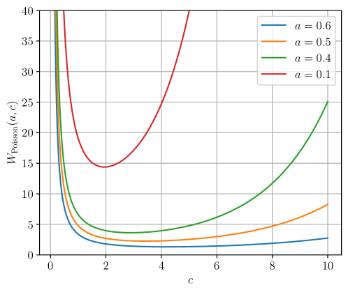
Figure 12: The scaled MFPT $W_{\text{Poisson}}(a,c)$ in the limit $b\to\infty$ (or equivalently $\sigma\to 0$ limit) plotted as a function of $c$ for different values of the parameter $a=R_{\rm tol}/L<1$. The MFPT exhibits a unique minimum at $c^{*}(a)$ that depends on $a$.

E.1.2 Finite $\sigma>0$

In this case, the parameter $b=L/\sigma$ is finite, and we have to evaluate the function $W_{\text{Poisson}}(a,b,c)$ in (85) numerically. For finite $b$, the scaled MFPT $\tau_{\text{Poisson}}=W(a,b,c)$ exhibits very different behavior as a function of $c$, for fixed $a$ and $b$. One of the biggest difference is that for finite $b$, as $c\to\infty$, the function $W_{\text{Poisson}}(a,b,c)$ now decays to zero, in stark contrast to the $b\to\infty$ case where it diverges (see (91)). Indeed, for finite $b$, one can extract the asymptotics behaviors of $W_{\text{Poisson}}(a,b,c)$ from (85) in the two limits $c\to 0$ and $c\to\infty$, by using the asymptotic behaviors of $K_{0}(z)$ given in (90). Skipping the details of the derivation we find

$$W_{\text{Poisson}}(a,b,c)\approx\begin{cases}&\frac{4\,A_{1}(a,b)}{c^{2}\,\ln(1/c)}\quad\,\,{\rm as}\quad c\to 0\\ \\ &\frac{4\,g(a,b)}{1-g(a,b)}\,\frac{1}{c^{2}}\quad\,\,{\rm as}\quad c\to\infty\end{cases}$$ (92)

where $g(a,b)$ is given in (84). The amplitude $A_{1}(a,b)$ can also be computed as

$$A_{1}(a,b)=\mathrm{e}^{-b^{2}/2}\,\int_{0}^{a\,b}\differential{z}z\,\mathrm{e}^{-z^{2}/2}\,\ln(z/{ab})\,I_{0}(b\,z)$$ (93)

One can check that in the limit $b\to\infty$, one obtains $A_{1}(a,b\to\infty)=\ln(1/a)$ and thus the first line in (92) coincides with the first line of (91).

In fact, as in the $d=1$ case, for finite but large $b$, $W_{\text{Poisson}}(a,b,c)$ as a function of $c$, first becomes a minimum at $c_{1}^{*}(a,b)$, then achieves a maximum at $c_{2}^{*}(a,b)$ and finally decays to zero as $1/c$ when $c\to\infty$. Thus, the minimum at $c_{1}^{*}(a,b)$ is metastable as in $d=1$. Finally, below a critical value $b<b_{c}(a)$, the curve $W_{\text{Poisson}}(a,b,c)$ decreases monotonically as a function of $c$, indicating that the metastable minimum disappears and the true optimal value is $c=\infty$ (corresponding to infinite resetting rate $r\to\infty$). In Fig. 13 we plot $W_{\text{Poisson}}(a,b,c)$ vs $c$ (for fixed $a=1/2$ and for different values of $b$)

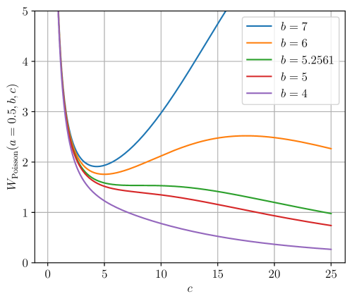
Figure 13: The scaled MFPT $W_{\text{Poisson}}(a,b,c)$ as a function of $c$ for fixed $a=1/2$ and different values of $b$. For $b>b_{c}(a)$, the curve shows a metastable minimum at $c_{1}^{*}(a,b)$, then a maximum at $c_{2}^{*}(a,b)$ and finally decreases monotonically to $0$ as $c\to\infty$. For $b<b_{c}(a)$, the scaled MFPT decreaes monotonically with $c$ with the only minimum at $c\to\infty$. The critical value is $b_{c}(a)\approx 5.2561$ for $a=1/2$.

E.2 Periodic Resetting

In this case, the MFPT is given by the exact formula (63) that reads

$$\langle t_{f}\rangle=\frac{\int_{0}^{T}Q_{0}(t)\differential{t}}{1-Q_{0}(T)}\,,$$ (94)

where $Q_{0}(t)$ is given explicitly in (75). We consider the Gaussian distribution for the resetting position: ${\cal P}({\vec{r}}_{0})=\mathrm{e}^{-{\vec{r}}_{0}^{2}/{2\sigma^{2}}}/{2\pi\sigma^{2}}$ and again define the dimensionless variables

$$\tau_{\text{periodic}}=\frac{4\,D\,\langle t_{f}\rangle}{L^{2}}\,;\quad\,\,a=\frac{R_{\rm tol}}{L}<1\,;\quad\,\,b=\frac{L}{\sigma}\,;\quad\,\,c=\frac{L}{\sqrt{4\,D\,T}}\,.$$ (95)

E.2.1 The limit $\sigma\to 0$: resetting to the origin

In this limit, we have ${\cal P}({\vec{r}}_{0})\to\delta({\vec{r}}_{0})$, corresponding to resetting to the origin. In terms of the dimensionless variables, we then have from (94)

$$\tau_{\text{periodic}}=W_{\text{periodic}}(a,c)=\frac{\displaystyle\frac{8\,a^{2}}{\pi}\int_{0}^{\infty}\frac{1-\mathrm{e}^{-x^{2}/{4\,a^{2}\,c^{2}}}}{x^{3}}\,\frac{Y_{0}(x/a)\,J_{0}(x)-J_{0}(x/a)\,Y_{0}(x)}{J_{0}^{2}(x)+Y_{0}^{2}(x)}\differential{x}}{\displaystyle 1-\frac{2}{\pi}\,\int_{0}^{\infty}\frac{\mathrm{e}^{-x^{2}/{4\,a^{2}\,c^{2}}}}{x}\,\frac{Y_{0}(x/a)\,J_{0}(x)-J_{0}(x/a)\,Y_{0}(x)}{J_{0}^{2}(x)+Y_{0}^{2}(x)}\differential{x}}$$ (96)

If we plot $W_{\text{periodic}}(a,c)$ vs. $c$, for fixed $a<1$, we again expect to see a unique minimum at $c^{*}(a)$, as in Fig. (12) for the Poisonian resetting. Unfortunately, numerical integration in (96) is rather hard as the intergrand is oscillatory and the integral is convergent but extremely slowly, in particular for large $c$. Indeed, it is easier to extract the behavior of $W_{\text{periodic}}(a,c)$ for small and large $c$ (for fixed $a$) directly from the Laplace transform, rather than from (96). We note that since $c=L/\sqrt{4DT}$, large (respectively small) $c$ corresponds to small (large) $T$. Hence we need to analyse $\langle t_{f}\rangle(T)$ in (94) for small and large $T$. For this we start with the Laplace transform ${\tilde{Q}_{0}}(s)$ in (74). For the resetting to the origin, using ${\cal P}({\vec{r}}_{0})\to\delta({\vec{r}}_{0})$, we get

$${\tilde{Q}}_{0}(s)=\int_{0}^{\infty}Q_{0}(t)\,\mathrm{e}^{-s\,t}\differential{t}=\frac{1}{s}\left[1-\frac{K_{0}\left(\sqrt{\frac{s}{D}}\,L\right)}{K_{0}\left(\sqrt{\frac{s}{D}}\,R_{\rm tol}\right)}\right]\,.$$ (97)

Small $T$ behavior of $\langle t_{f}\rangle$: To extract the small $t$ asymptotics of $Q_{0}(t)$, we need to analyse the Laplace transform ${\tilde{Q}}_{0}(s)$ in (97) for large $s$. Using $K_{0}(z)\approx\sqrt{\pi/{(2\,z)}}\,\mathrm{e}^{-z}$ for large $z$, we get for large $s$

$${\tilde{Q}}_{0}(s)\approx\frac{1}{s}\left[1-\sqrt{a}\,\mathrm{e}^{-\sqrt{\frac{s}{D}}\,(L-R_{\rm tol})}\right]\,,$$ (98)

where $a=R_{\rm tol}/L$. The Laplace transform can now be explicitly inverted to give for small $t$

$$Q_{0}(t)\approx 1-\sqrt{a}\,\operatorname{erfc}\left(\frac{L-R_{\rm tol}}{\sqrt{4Dt}}\right)\,,$$ (99)

where $\operatorname{erfc}(z)=(2/{\sqrt{\pi}})\,\int_{0}^{z}\mathrm{e}^{-u^{2}}\,du$ is the complementary error function. It has the following asymptotic behavior for large argument $\operatorname{erfc}(z)\approx\mathrm{e}^{-z^{2}}/{z\,\sqrt{\pi}}$. Now, from (94), we get for small $T$ (using (99) and keeping only leading order terms for small $T$)

$$\langle t_{f}\rangle=\frac{\int_{0}^{T}Q_{0}(t)\differential{t}}{1-Q_{0}(T)}\approx\frac{T}{\sqrt{a}}\,\operatorname{erfc}\left(\frac{L-R_{\rm tol}}{\sqrt{4DT}}\right)\,.$$ (100)

Finally, using the asymptotics of $\operatorname{erfc}(z)$ for large $z$ in (100), we can express, after a few steps of straightforward algebra, the scaled MFPT $\tau_{\text{periodic}}$ for small $T$, or equivalently for large $c$, in terms of adimensional variables in (95)

$$\tau_{\text{periodic}}=W_{\text{periodic}}(a,c)=\frac{4\,D\,\langle t_{f}\rangle}{L^{2}}\approx\frac{\sqrt{\pi}\,(1-a)}{\sqrt{a}\,c}\,\mathrm{e}^{(1-a)^{2}\,c^{2}}\,;\quad{\rm as}\quad c\to\infty\,.$$ (101)

Thus, $W_{\text{periodic}}(a,c)$, for fixed $a$, diverges very fast as $c\to\infty$. Let us remark that deriving this asymptotic behavior directly from the expression in (96) is rather hard.

Large $T$ behavior of $\langle t_{f}\rangle$: To compute the large $t$ behavior of $Q_{0}(t)$, we need to analyse the small $s$ behavior of ${\tilde{Q}}_{0}(s)$ in (97). Fortunately this large $t$ behavior is well known Barzykin and Tachiya (1993) and one gets

$$Q_{0}(t)\approx\frac{2\ln(1/a)}{\ln\left(\frac{4Dt}{L^{2}\,a^{2}}\right)}\,;\quad{\rm for}\quad t\gg L^{2}\,$$ (102)

where $a=R_{\rm tol}/L<1$. Substituting this result in (94), we get for large $T$, i.e., small $c=L/\sqrt{4DT}$ the following result

$$\langle t_{f}\rangle\approx 2\,a^{2}\,\ln(1/a)\,\int_{0}^{1/{(c\,a)^{2}}}\frac{\differential{z}}{\ln z}\,.$$ (103)

We can easily evaluate the integral for large $c$. Finally the scaled MFPT for small $c$ is given by (keeping only the leading asymptotic behavior)

$$\tau_{\text{periodic}}=W_{\text{periodic}}(a,c)\approx\frac{\ln(1/a)}{c^{2}\,\ln(1/{ca})}\,;\quad{\rm as}\quad c\to 0$$ (104)

Thus, summarizing for the $\sigma=0$ (or $b\to\infty$) case of the periodic resetting, the scaled MFPT, as a function of $c$ has the following limiting behaviors

$$\tau_{\text{periodic}}=W_{\text{periodic}}(a,c)\approx\begin{cases}&\frac{\ln(1/a)}{c^{2}\,\ln(1/{ca})}\,;\quad{\rm as}\quad c\to 0\\ \\ &\frac{\sqrt{\pi}\,(1-a)}{\sqrt{a}\,c}\,\mathrm{e}^{(1-a)^{2}\,c^{2}}\,;\quad{\rm as}\quad c\to\infty\end{cases}$$ (105)

Thus $W_{\text{periodic}}(a,c)$, as a function of $c$ for fixed $a<1$, diverges as the both ends $c\to 0$ and $c\to\infty$. It has a unique minimum at some $c=c^{*}(a)$. As mentioned before, plotting directly the full function $W(a,c)$ as given explicitly in (96) turns out to be hard, due to the oscillatory and exponential nature of the integrands. Using a few numerical tricks, we managed to plot $W_{\text{periodic}}(a,c)$ vs. $c$ for different values of $a$ as shown in Fig. (14).

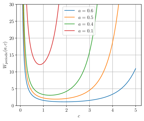
Figure 14: The scaled MFPT $W_{\text{periodic}}(a,c)$ in the limit $b\to\infty$ (or equivalently $\sigma\to 0$ limit) plotted as a function of $c$ for different values of the parameter $a=R_{\rm tol}/L<1$. The MFPT exhibits a unique minimum at $c^{*}(a)$ that depends on $a$.

To perform the numerical integration of (96), we must extract out the divergences of the integrands in order to improve precision. Indeed, the denominator becomes tends to zero exponentially quicky when $c$ increases, so an accurate integration of the denominator integral is crucial. To do that, we expand the integrand around $x=0$ as

$$f_{1}(x)=\tfrac{Y_{0}(x/a)J_{0}(x)-Y_{0}(x)J_{0}(x/a)}{J_{0}(x)^{2}+Y_{0}(x)^{2}}\frac{1}{x}\mathrm{e}^{-x^{2}/4a^{2}c^{2}}\underset{x\rightarrow 0}{\simeq}\tfrac{2}{\pi}\ln\left(\tfrac{1}{a}\right)\frac{1}{x}\frac{1}{1+\frac{4}{\pi^{2}}\left(\gamma+\ln\tfrac{x}{2}\right)^{2}}=:f_{2}(x)$$

Happily, the integral of $f_{2}$ is analytical. The denominator can be rewritten

$$1-\frac{2}{\pi}\int_{0}^{\infty}\differential{x}f_{1}(x)=1-\frac{2}{\pi}\int_{0}^{\infty}\differential{x}(f_{1}(x)-f_{2}(x))-2\ln\left(\frac{1}{a}\right)$$

where $\int_{0}^{\infty}\differential{x}(f_{1}(x)-f_{2}(x))$ is much easier to compute numerically. Still, this is not enough, because the integrand now converges slowly when $x\rightarrow\infty$, preventing good precision. Fortunately, because $f_{1}$ decays exponentially, we can cut off the integral ($x_{c}=c^{2}$ seems to be a good cutoff), and because $\int_{0}^{x_{c}}\differential{x}f_{2}(x)$ is still analytical, we can rewrite the denominator as

$$1-\frac{2}{\pi}\int_{0}^{\infty}\differential{x}f_{1}(x) \approx 1-\frac{2}{\pi}\int_{0}^{x_{c}}\differential{x}f_{1}(x)$$

$$= 1-\frac{2}{\pi}\int_{0}^{x_{c}}\differential{x}(f_{1}(x)-f_{2}(x))-\frac{2}{\pi}\int_{0}^{x_{c}}\differential{x}f_{2}(x)$$

$$= 1-\frac{2}{\pi}\int_{0}^{x_{c}}\differential{x}(f_{1}(x)-f_{2}(x))-\ln\left(\tfrac{1}{a}\right)\left(1+\tfrac{2}{\pi}\arctan\left(\tfrac{2}{\pi}\left(\gamma+\ln\tfrac{x_{c}}{2}\right)\right)\right)$$

The remaining integral of $f_{1}-f_{2}$ is easy to compute accurately. The same regularization can be used for the numerator.

E.2.2 Finite $\sigma>0$

For finite $\sigma$, we have ${\cal P}({\vec{r}}_{0})=\mathrm{e}^{-{\vec{r}}_{0}^{2}/{2\sigma^{2}}}/{2\pi\sigma^{2}}$ and our main objective is to evaluate $Q_{0}(t)$ in (75) and then use (94) to compute $\langle t_{f}\rangle$. Thus the main technical challenge is to evaluate the integral over ${\vec{r}}_{0}$ in (75). We consider first the following integral

$$I_{1}=\int\differential{\vec{r}_{0}}{\cal P}({\vec{r}}_{0})\,Y_{0}\left(x\,\frac{|{\vec{r}}_{0}-L|}{R_{\rm tol}}\right)\,.$$ (106)

We first make the change of variable ${\vec{r}}_{0}-{\vec{R}}_{\rm tar}=\vec{R}$, denote $L=|{\vec{R}}_{\rm tar}|$, and shift to the polar coordinates. This gives

$$I_{1} = \frac{1}{2\,\pi\,\sigma^{2}}\,\int_{R>R_{\rm tol}}\int_{0}^{2\pi}\mathrm{e}^{-({\vec{R}}_{\rm tar}+{\vec{R}})^{2}/{2\sigma^{2}}}\,Y_{0}\left(x\,\frac{R}{R_{\rm tol}}\right)\,R\,\differential{R}\differential{\theta}$$ (107)

$$= \frac{\mathrm{e}^{-L^{2}/{2\sigma^{2}}}}{2\,\pi\,\sigma^{2}}\,\int_{R_{\rm tol}}^{\infty}\differential{R}R\,\mathrm{e}^{-R^{2}/{2\sigma^{2}}}Y_{0}\left(x\,\frac{R}{R_{\rm tol}}\right)\,\int_{0}^{2\pi}\mathrm{e}^{-L\,R\,\cos(\theta)/\sigma^{2}}\,\differential{\theta}$$

$$= \frac{\mathrm{e}^{-L^{2}/{2\sigma^{2}}}}{\sigma^{2}}\,\int_{R_{\rm tol}}^{\infty}\differential{R}R\,\mathrm{e}^{-R^{2}/{2\sigma^{2}}}\,Y_{0}\left(x\,\frac{R}{R_{\rm tol}}\right)\,I_{0}\left(\frac{R\,L}{\sigma^{2}}\right)\,.$$

Similarly, we have

$$I_{2}=\int\differential{\vec{r}_{0}}{\cal P}({\vec{r}}_{0})\,J_{0}\left(x\,\frac{|{\vec{r}}_{0}-\vec{R}_{\text{tar}}|}{R_{\rm tol}}\right)=\frac{\mathrm{e}^{-L^{2}/{2\sigma^{2}}}}{\sigma^{2}}\,\int_{R_{\rm tol}}^{\infty}\differential{R}R\,\mathrm{e}^{-R^{2}/{2\sigma^{2}}}\,J_{0}\left(x\,\frac{R}{R_{\rm tol}}\right)\,I_{0}\left(\frac{R\,L}{\sigma^{2}}\right)\,.$$ (108)

Putting all these results in (75), and further rescaling $R=\sigma\,z$ we can write $Q_{0}(t)$ in terms of dimensionless variables $a=R_{\rm tol}/L$ and $b=L/\sigma$ in a somewhat compact form

$$Q_{0}(t)=\frac{2}{\pi}\,\mathrm{e}^{-b^{2}/2}\,\int_{0}^{\infty}\differential{x}\frac{\mathrm{e}^{-D\,t\,x^{2}/R_{\rm tol}^{2}}}{x}\,\frac{J_{0}(x)\,F_{1}(x,a,b)-Y_{0}(x)\,F_{2}(x,a,b)}{J_{0}^{2}(x)+Y_{0}^{2}(x)}\,$$ (109)

where we have defined

$$F_{1}(x,a,b) = \int_{a\,b}^{\infty}\differential{z}z\,\mathrm{e}^{-z^{2}/2}\,Y_{0}\left(\frac{x\,z}{a\,b}\right)\,I_{0}(b\,z)$$ (110)

$$F_{2}(x,a,b) = \int_{a\,b}^{\infty}\differential{z}z\,\mathrm{e}^{-z^{2}/2}\,J_{0}\left(\frac{x\,z}{a\,b}\right)\,I_{0}(b\,z)$$ (111)

Finally, substituting the expression (109) of $Q_{0}(t)$ in (94) we can obtain the expression of $\langle t_{f}\rangle$ and eventually that of the scaled MFPT for finite $\sigma$, i.e., for finite $b$, in terms of $a$, $b$ and $c=L/\sqrt{4\,D\,T}$. We get the following exact expression

$$\tau_{\text{periodic}}=\frac{4\,D\,\langle t_{f}\rangle}{L^{2}}\equiv W_{\text{periodic}}(a,b,c)=\frac{\displaystyle\frac{8\,a^{2}}{\pi}\,\mathrm{e}^{-b^{2}/2}\int_{0}^{\infty}\frac{1-\mathrm{e}^{-x^{2}/{4\,a^{2}\,c^{2}}}}{x^{3}}\,\frac{J_{0}(x)\,F_{1}(x,a,b)-Y_{0}(x)\,F_{2}(x,a,b)}{J_{0}^{2}(x)+Y_{0}^{2}(x)}\differential{x}}{\displaystyle 1-\frac{2}{\pi}\,\mathrm{e}^{-b^{2}/2}\,\int_{0}^{\infty}\frac{\mathrm{e}^{-x^{2}/{4\,a^{2}\,c^{2}}}}{x}\,\frac{J_{0}(x)\,F_{1}(x,a,b)-Y_{0}(x)\,F_{2}(x,a,b)}{J_{0}^{2}(x)+Y_{0}^{2}(x)}\differential{x}}$$ (112)

where $F_{1}(x,a,b)$ and $F_{2}(x,a,b)$ are given respectively in (110) and (111). Note that the result for $b\to\infty$ limit, i.e., $\sigma=0$ case is given in (96). The result in (112) is the finite $b$ analogue of (96). Plotting $W_{\text{periodic}}(a,b,c)$ vs. $c$, for fixed $a<1$ and $b$, is challenging, and similar numerical tricks are used to numerically integrate it. In particular, the integral in the denominator can be re-written as

$$I_{\text{den}}\simeq\mathrm{e}^{-\frac{b^{2}}{2}}\int_{0}^{x_{c}}\differential{x}\int_{ab}^{\infty}\differential{z}z\mathrm{e}^{-\frac{z^{2}}{2}}I_{0}(bz)(f_{1}-f_{2})+\Big{(}\tfrac{\pi}{2}+\arctan\big(\tfrac{2}{\pi}\left(\gamma+\ln\tfrac{x_{c}}{2}\right)\big{missing})\Big{)}A_{1}(b,z)$$

where $A_{1}$ is defined bellow, $f_{1}$ and $f_{2}$ are as before but with $\ln(z/ab)$ in place of $\ln(1/a)$, and where the remaining double integral is relatively easy to compute accurately. To test the integration, we compared the results to the asymptotic behaviors in Eq. (113). The results are plotted in Fig. (15).

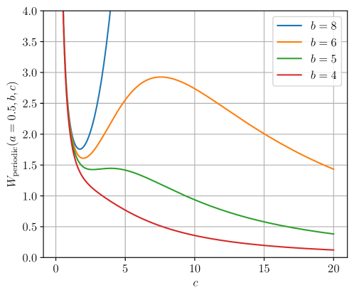
Figure 15: The scaled MFPT $W_{\rm per}(a,b,c)$ as a function of $c$ for fixed $a=1/2$ and different values of $b$. For $b>b_{c}(a)$, the curve shows a metastable minimum at $c_{1}^{*}(a,b)$, then a maximum at $c_{2}^{*}(a,b)$ and finally decreases monotonically to $0$ as $c\to\infty$. For $b<b_{c}(a)$, the scaled MFPT decreaes monotonically with $c$ with the only minimum at $c\to\infty$. The critical value is $b_{c}(a)\approx 5$ for $a=1/2$.

As in the Poissonian case, if we plot $W_{\text{periodic}}(a,b,c)$ vs. $c$, for fixed $a<1$ and $b$, we expect to see a minimum at $c_{1}^{*}(a,b)$, followed by a maximum at $c_{2}^{*}(a,b)>c_{1}^{*}(a,b)$ and then an absolute minimum at $c\to\infty$. The metstable minimum $c_{1}^{*}(a,b)$ disappears below a critical value $b<b_{c}(a)$, as in the Poissonian case. Thus, for any finite $b$, the function $W_{\text{periodic}}(a,b,c)$ vs $c$ finally decays to $0$ as $c\to\infty$. This is in stark contrast to the $b\to\infty$ case, where we recall that $W_{\text{periodic}}(a,\infty,c)=W_{\text{periodic}}(a,c)$ diverges as $c\to\infty$ (see the (105)). It would be nice to see this decay at large $c$ by plotting $W_{\text{periodic}}(a,b,c)$ vs. $c$ in (112). However, as mentioned earlier, plotting this function is hard since the numerical integration in (112) converges very slowly, in particular for large $c$.

Indeed, it is easier to extract the behavior of $W_{\text{periodic}}(a,b,c)$ for small and large $c$ (with fixed $a$ and $b$) directly from the Laplace transform, rather than from (112). We note that since $c=L/\sqrt{4DT}$, large (respectively small) $c$ corresponds to small (large) $T$. Hence we need to analyse $\langle t_{f}\rangle(T)$ in (94) for small and large $T$. For this we start with the Laplace transform ${\tilde{Q}_{0}}(s)$ in (74) and analyse its small $s$ and large $s$ behaviors, as we have done before in the $\sigma=0$ (or $b\to\infty$ limit) case. Skipping details, we just write the final results

$$W_{\text{periodic}}(a,b,c)\approx\begin{cases}&\frac{A_{1}(a,b)}{c^{2}\,\ln\left(\frac{1}{c\,a}\right)}\quad\,\,{\rm as}\quad c\to 0\\ \\ &\frac{g(a,b)}{1-g(a,b)}\,\frac{1}{c^{2}}\quad\,\,{\rm as}\quad c\to\infty\end{cases}$$ (113)

where $I_{0}(z)$ is the modified Bessel function of the first kind and the amplitude $A_{1}(a,b)$ already appeared in (93) and reads

$$A_{1}(a,b)=\mathrm{e}^{-b^{2}/2}\,\int_{a\,b}^{\infty}\differential{z}z\,\mathrm{e}^{-z^{2}/2}\,\ln\left(\frac{z}{a\,b}\right)\,I_{0}(b\,z)\,.$$ (114)

Thus, for fixed $b$ finite and fixed $a<1$, the scaled MFPT $W_{\text{periodic}}(a,b,c)$ decays for large $c$ as $c\to\infty$, in contrast to the $b\to\infty$ case where it diverges as $c\to\infty$ (as in (105)). Thus the true optimal value of $c$ occurs at $c\to\infty$, even though there is a metastable minimum at an earlier value $c_{1}^{*}(a,b)$ for $b>b_{c}(a)$.

Appendix F Anisotropy of the initial position distribution

To quantify the effect of initial position anisotropy, which is unfortunately important with our experimental setup, we performed simulations with an non-symetric gaussian initial position distribution where $\sigma_{x}\neq\sigma_{y}$. Fig. 16 shows that for $a=0.5$, the mismatch induced is about $\pm 15\%$ for a $20\%$ anisotropy. Moreover, it is about $\pm 10\%$ and $\pm 20\%$ for $a=0.9$ and $a=0.3$ respectively. As expected, the MFPT is decreased when $\sigma_{x}>\sigma_{y}$. The effect is more pronounced at high $c$, i.e. for frequent resetting, especially when $a$ approaches $1$. Many more figures at available at https://github.com/xif-fr/BrownianMotion/tree/master/langevin-mfpt.

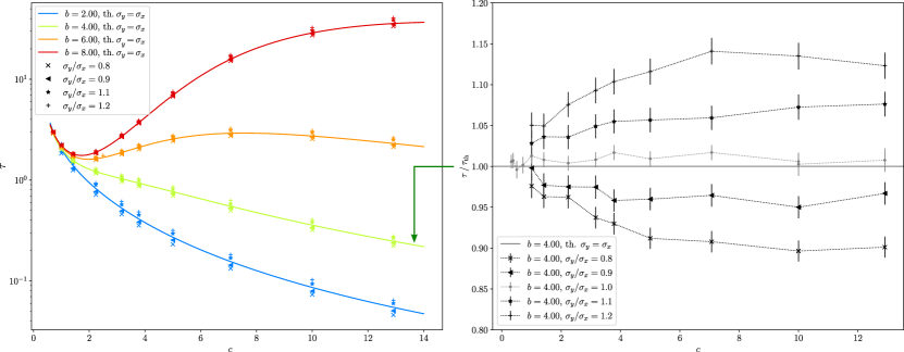
Figure 16: Simulation. Effect of anisotropy of the initial position distribution on the MFPT. Example with $a=0.5$ and periodic resetting, where $\sigma_{y}/\sigma_{x}$ is varied from 0.8 to 1.2, and $b$ from 8 to 2. Left : $\tau$ as a function of $c$ for several anisotropies (points) againt the theoretical MFPT (solid lines). Right : deviation (points) relative to theory (solid line) for several anisotropies.

Fig. 17 represents the 2D experimental data with periodic resetting against the theory using

$$\sigma=\sigma_{\text{mean}}=\sqrt{\frac{\sigma_{x,\text{exp}}^{2}+\sigma_{y,\text{exp}}^{2}}{2}}\,.$$

The mismatch is more pronounced than with $\sigma=\sigma_{x,\text{exp}}$, confirming the choice made in Section IV.1.2.

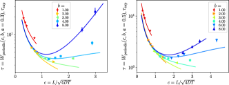
Figure 17: Experiment. $\tau$ versus $c$ for the periodic resetting protocol in 2D for finite $b$ and $a=0.3$ (top panel) and $a=0.5$ (bottom panel). Continuous lines are the the theoretical predictions of Eq. 112 with $\sigma=\sigma_{\text{mean}}$ and the symbols corresponds to the results obtained from the experimental data.

Appendix G Numerical integration of the Langevin equation

To measure numerically the MFPT, we integrate the Langevin equation :

$$\dot{x}(t)=\sqrt{2\,D}\,\eta_{x}(t),\quad\dot{y}(t)=\sqrt{2\,D}\,\eta_{y}(t)$$ (115)

where $D$ is the diffusion constant (which we set equal to 1) and $\eta_{m}$ ($m=x,y$) are delta correlated noises with $\langle\eta_{m}(t)\eta_{m}(t^{\prime})\rangle=\delta(t-t^{\prime})$ and $\langle\eta_{m}(t)\eta_{m^{\prime}}(t)\rangle=0$ for $m\neq m^{\prime}$. The simulation starts with $x(0),y(0)$ randomly drawn from a Gaussian distribution of standard deviation $\sigma$. The particle freely diffuses till a time $T$ which can be either constant (periodic reset) or randomly distributed (poissonian reset), and $x,y$ are reset at a new random position, drawn from the same Gaussian distribution. The cycle is repeated utill the target is reached (a line at $x=L$ in 1 dimension, and a circle of radius $R_{\text{tol}}$ centered at $x=L$ in 2 dimensions). The first passage time $t_{\text{f}}$ is then recorded. The integration step is fixed at a small enough value so as the systematic error introduced by the time discretization on $\langle t_{\text{f}}\rangle$ is typically smaller or equal to 1%. To compute the MFPT $\langle t_{\text{f}}\rangle$, between $N=20000$ and 200000 trajectories (representing about $2\,\mathrm{hour}\cdot\mathrm{core}$ for a typical 2015 CPU) are computed for each $(a,b,c)$. Multiple values of $(L,R_{\text{tol}},\sigma,T|\alpha)$ are possible for each $(a,b,c)$, and we checked that the resulting adimentionalized MFPT $\tau$ does not depend on these values, but only on $(a,b,c)$ (withing a 5% error margin maximum, typically 1%). The uncertainty on the MFPT ($\operatorname{std}(t_{\text{f}})/\sqrt{N}$) is typically $<1\%$, which is too small for the error bars in figures 7,10,11 to be visible.

The code is available at https://github.com/xif-fr/BrownianMotion/.