Diquark properties from full QCD lattice simulations

Abstract

We study diquarks on the lattice in the background of a static quark, in a gauge-invariant formalism with quark masses down to almost physical $m_{\pi}$. We determine mass differences between diquark channels as well as diquark-quark mass differences. The lightest and next-to-lightest diquarks have “good” scalar, $\bar{3}_{F}$, $\bar{3}_{c}$, $J^{P}=0^{+}$, and “bad” axial vector, $6_{F}$, $\bar{3}_{c}$, $J^{P}=1^{+}$, quantum numbers, and a bad-good mass difference for $ud$ flavors, $198(4)~{}\rm{MeV}$, in excellent agreement with phenomenological determinations. Quark-quark attraction is found only in the “good” diquark channel. We extract a corresponding diquark size of $\sim 0.6~{}\rm{fm}$ and perform a first exploration of the “good” diquark shape, which is shown to be spherical. Our results provide quantitative support for modeling the low-lying baryon spectrum using good light diquark effective degrees of freedom.

1 Introduction

The renewed popularity (e.g. Jaffe:2004ph ; Ali:2017jda ; Barabanov:2020jvn ) of the old diquark ideaGellMann:1964nj ; Ida:1966ev ; Lichtenberg:1982jp makes a detailed ab initio lattice study useful and timely.

Diquarks, like quarks, carry an open color index, and hence do not exist as asymptotic states. Since contracting a diquark with a quark produces a baryon operator, a diquark with an anti-diquark a tetraquark operator, etc., effective diquark degrees of freedom may be useful building blocks for phenomenological descriptions of hadronic states. Such a description might prove successful if diquarks are compact objects with fewer degrees of freedom than the quark pairs they represent. The phenomenological success of diquark models Cahill:1987qr ; Maris:2002yu ; Santopinto:2004hw ; Barabanov:2020jvn supports this possibility, provided one assumes the diquarks have “good” ($\bar{3}_{F}$, $\bar{3}_{c}$, $J^{P}=0^{+}$) flavor, color and Dirac quantum numbers. This assumption is natural since both one-gluon-exchange DeRujula:1975qlm ; DeGrand:1975cf and instanton interactions tHooft:1976snw ; Shuryak:1981ff ; Schafer:1996wv are attractive in this channel. The present work aims to investigate this picture quantitatively by studying diquark masses, sizes and spatial correlations using first-principle lattice QCD simulations.

Since diquarks are colored, and not gauge-invariant, neither are their properties. One way to deal with this issue is to work in a fixed gauge, typically Landau gauge or a variant thereof, see, e.g., the lattice studies of Refs. Hess:1998sd ; Bi:2015ifa ; Babich:2007ah . The drawback is that the resulting diquark properties depend on the gauge choice. This problem is well known for the size determination Teo:1992zu ; Negele:2000uk ; Alexandrou:2002nn , though diquark masses, and even mass differences, are also affected since these are extracted from the temporal decay rates of appropriate correlators, which will change in a gauge non-local in time like Landau gauge. Alternately, one can introduce a static color source which, together with the diquark, forms a color singlet baryon, whose mass is gauge-invariant. Since the mass of such a static-light-light baryon diverges in the continuum limit, the quantities of interest are mass differences between various diquark channels. The diquark size can also be obtained in a gauge-invariant way, from the spatial decay rate of the quark density-density correlator at fixed time Orginos:2005vr ; Alexandrou:2005zn ; Alexandrou:2006cq ; Green:2010vc ; Green:2012zza ; Fukuda:2017mmh .

We adopt the second, gauge-invariant approach of Alexandrou:2005zn ; Alexandrou:2006cq ; Fukuda:2017mmh . Measurements are taken on dynamical $n_{f}=2+1$, $32^{3}\times 64$, clover-improved Wilson fermion gauge configurations with lattice spacing $a\approx 0.090~{}\rm{fm}$ generated by PACS-CS Aoki:2008sm ; Namekawa:2013vu and publicly available from the JLDG repository JLDG . Five ensembles, with pion masses $m_{\pi}=164,299,415,575,707$ MeV, are considered, allowing us to study the dynamical light-quark mass dependence of diquark properties and perform a short, controlled extrapolation to physical $m_{\pi}$. We re-use the (gauge-fixed, wall-source) quark propagators from Francis:2016hui ; Francis:2018jyb . To connect with previous quenched studies, we also employ a new $32^{3}\times 64$, $a\approx 0.092~{}\rm{fm}$, quenched ensemble with valence pion mass $m_{\pi}=909~{}\rm{MeV}$. Static quark propagators are computed using the method of DellaMorte:2005nwx ; Donnellan:2010mx with HYP1 smearing. See Appendix B for further details.

2 Diquark spectroscopy

We first quantify the expected reduction in the “good” diquark mass by studying the static-light-light baryon spectrum. With $Q$ the static quark, $c,C$ denoting charge conjugation, and light quarks in a $D_{\Gamma}=q^{c}C\Gamma q$ diquark configuration, where $\Gamma$ acts in Dirac space, we measure the baryon correlators

$$C_{\Gamma}(t)=\sum_{\vec{x}}\Big{\langle}[D_{\Gamma}Q](\vec{x},t)~{}[D_{\Gamma}Q]^{\dagger}(\vec{0},0)\Big{\rangle}\,.$$ (1)

$\Gamma=\gamma_{5}$, $\gamma_{5}\gamma_{0}$ for “good”, $0^{+}$ diquarks, $\gamma_{i}$ for “bad”, $1^{+}$ diquarks, and $\bf{1}$ and $\gamma_{5}\gamma_{i}$, for the “not-even-bad”, odd-parity $0^{-}$ and $1^{-}$ diquarks. We also measure the correlators of static-light meson operators $[\bar{Q}\Gamma q]$. The static quark $(m_{Q}\rightarrow\infty)$ acts as a spectator; its mass cancels in mass differences, exposing the diquark spectrum.

We consider diquarks with light-light $(ud)$, light-strange $(\ell s$, $\ell=u,d)$ and strange-strange^′ $(ss^{\prime})$ flavors on 5 ensembles with different light-quark, hence pion, masses. Note in particular that $s^{\prime}$ denotes a hypothetical additional strange valence quark. It is introduced to allow a study of a good diquark with both quarks having the same (strange) quark mass, which the good diquark flavor antisymmetry makes inaccessible to two identical $s$ quarks. Technical aspects of the analysis are summarized in App. C.

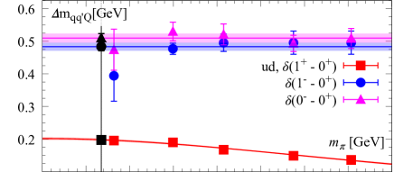
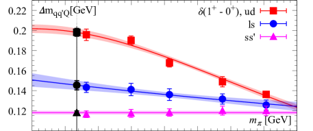
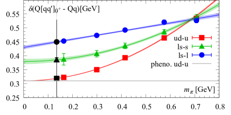
Figure 1: Diquark spectroscopy: diquark mass differences as a function of $m_{\pi}$. Vertical lines identify physical $m_{\pi}$. The colored bands show the results from fitting to the ansätze described in the text. (Top) The $ud$ differences $\delta(1^{+}-0^{+})$, $\delta(1^{-}-0^{+})$ and $\delta(0^{-}-0^{+})$. (Middle) Bad-good $ud$, $\ell s$ and $ss^{\prime}$ differences, extrapolated to physical $m_{\pi}$ using Eq. (2). (Bottom) Analogous $Qqq-\bar{Q}q$ differences, extrapolated using Eq. (3). The horizontal line is the phenomenological value $\delta(b[ud]_{0^{+}}-\bar{b}u)=306~{}\rm{MeV}$.

Figure 1 (top panel) shows the dependence on $m_{\pi}$ of the $ud$ $0^{+}$ versus $1^{+}$, $0^{-}$ and $1^{-}$ diquark mass differences. The results provide quantitative support for the phenomenological diquark approach, which considers only good $0^{+}$ diquarks. Explicitly, the good $0^{+}$ $ud$ diquark lies lowest in the spectrum, 100-200 MeV below the bad $1^{+}$ $ud$ diquark. The negative-parity $0^{-}$ and $1^{-}$ $ud$ diquarks lie even higher, $\sim 0.5~{}\rm{GeV}$ above the good diquark and will thus play no role in the low-energy physics. The same pattern is observed in the $\ell s$ and $ss^{\prime}$ sectors. Figure 1 (middle panel) compares the $ud$, $\ell s$ and $ss^{\prime}$ $(1^{+}-0^{+})$ splittings. The curves in Fig. 1 are fits using Ansätze guided by limiting cases. Explicitly, the $(1^{+}-0^{+})$ mass difference goes to a constant in the chiral limit and decreases as $1/(m_{q_{1}}m_{q_{2}})$, with $m_{\pi}\sim(m_{q_{1}}+m_{q_{2}})$, in the heavy-quark limit. The simplest interpolation between these limits is the two-parameter form

$$\delta(1^{+}-~{}0^{+})_{q_{1}q_{2}}=A/\left[1+\big{(}m_{\pi}/B\big{)}^{n}\right],$$ (2)

with $n=0,1,2$ for $q_{1}q_{2}=ss^{\prime}$, $\ell s$ and $ud$, respectively. Here, $A$ fixes the chiral limit behavior, while $B$ separates the light- and heavy-quark regimes. The fits clearly describe the data very well. A similar Ansatz proposed in Alexandrou:2005zn , with $n$ twice as large, produces a much poorer fit. Note that the $ud$, $\ell s$ and $ss^{\prime}$ curves all intersect at the flavor-symmetric $n_{f}=3$ point, $m_{u,d}\rightarrow m_{s}$. The parameter values and physical-point mass differences are listed in the top half of Table 1. The latter are in excellent agreement with phenomenological expectations Jaffe:2004ph (see App. A).

Further information on the diquark spectrum is provided by the mass splittings between static $Qqq^{\prime}$ baryons and the corresponding static $\bar{Q}q$, $\bar{Q}q^{\prime}$ mesons. Results for the $Qud-\bar{Q}u$, $Q\ell s-\bar{Q}\ell$ and $Q\ell s-\bar{Q}s$ combinations are shown in the bottom panel of Fig. 1, together with fits to the Ansatz,

$$\delta(Q[q_{1}q_{2}]_{0^{+}}-\bar{Q}q_{2})=C~{}\left[1+(m_{\pi}/D)^{n}\right]\,,$$ (3)

where $C$ fixes the chiral limit value and $D$ separates the light- and heavy-$q_{1}$ quark regimes. In the latter, the mass splitting must grow linearly with the mass $m_{q_{1}}$, which dictates $n=1$ if $q_{1}$ is a heavy quark, $n=2$ otherwise. The bottom half of Tab. 1 lists the fit parameter values and resulting extrapolated physical-point mass differences.

The excellent agreement with phenomenological expectations of our results for all of the $\delta(1^{+}-0^{+})_{ud}$, $\delta(1^{+}-0^{+})_{us}$, $\delta(Q[ud]_{0^{+}}-\bar{Q}u)$ and $\delta(Q[ud]_{0^{+}}-\bar{Q}u)$ splittings, detailed in App. A, provides strong evidence that we have successfully identified the ground-state heavy baryon signals and that, as expected, residual discretization effects are small. This justifies investigating the structure of the diquark correlations in those baryon ground states using fixed-time density-density correlators, described in more detail below. Appendix A also provides a brief outline of other approaches that have been used to estimate the good-bad diquark splittings.

An additional interesting relation between the bad-good diquark and $\Delta-N$ splittings is discussed in App. C.

All in [GeV]	$\delta E(m_{\pi}^{\rm{phys}})~{}~{}$	A	B
$\delta(1^{+}-~{}0^{+})_{ud\,}$	0.198(4)	0.202(4)	1.00(5)
$\delta(1^{+}-~{}0^{+})_{\ell s\,}$	0.145(5)	0.151(7)	3.7(15)
$\delta(1^{+}-~{}0^{+})_{ss^{\prime}}$	0.118(2)	0.118(2)
		C	D
$\delta(Q[ud]_{0^{+}}-\bar{Q}u)$	0.319(1)	0.310(1)	0.814(8)
$\delta(Q[\ell s]_{0^{+}}-\bar{Q}s)$	0.385(9)	0.379(10)	1.09(6)
$\delta(Q[\ell s]_{0^{+}}-\bar{Q}\ell)$	0.450(6)	0.430(6)	2.95(35)

Table 1: Fit parameters $A,B,C,D$ and physical-point bad-good diquark (top half) and good diquark-quark (bottom half) mass differences, the errors are statistical only. Here the indices $ud$, $\ell s$, $ss^{\prime}$ signify the different flavor combinations, with $s^{\prime}$ denoting a hypothetical additional valence strange quark (see Sec. 2). For a detailed discussion of the fit ansätze, we refer to the text. Further information on phenomenological results can be found in App. A.

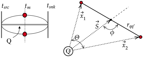
Figure 2: Sketch of the density correlators. (Left) 2D temporal view. (Right) Current insertions, spatial view.

3 Diquark structure

Having successfully identified the relevant ground-state baryon signals, we now turn to an investigation of the light diquark structures in those states. To do so, we compute the fixed-time density-density correlators:

$$C_{\Gamma}^{dd}(\vec{x}_{1},\vec{x}_{2},t)=\Big{\langle}\mathcal{O}_{\Gamma}(\vec{0},2t)\rho(\vec{x}_{1},t)\rho(\vec{x}_{2},t)\mathcal{O}_{\Gamma}^{\dagger}(\vec{0},0)\Big{\rangle}$$ (4)

where $\rho(\vec{x},t)=\bar{q}(\vec{x},t)\gamma_{0}q(\vec{x},t)$ and $\mathcal{O}_{\Gamma}$ are the baryon operators used before. $\Gamma$ characterizes the diquark channel. With the static quark at the origin, the light-quark source and sink points are $(\vec{0},t_{src})$ and $(\vec{0},t_{snk})$. The currents are inserted at $t_{m}=(t_{snk}+t_{src})/2$ to maximize projection onto the ground state. The relative positions of the static source and current insertions $\vec{x}_{1}$, $\vec{x}_{2}$, can be characterized by $\vec{r}_{qq^{\prime}}=\vec{x}_{2}-\vec{x}_{1}$, $\vec{S}=(\vec{x}_{1}+\vec{x}_{2})/2$, the separation between the static source and diquark midpoint, and $\phi$, the angle between $\vec{r}_{qq^{\prime}}$ and $\vec{S}$, as shown in Fig. 2. We define

$$\rho_{2}(r_{qq^{\prime}},S,\phi;\Gamma)\equiv C^{dd}_{\Gamma}(\vec{x}_{1},\vec{x}_{2},t_{m})\,,$$ (5)

dropping the label $\Gamma$ when this produces no confusion.

For fixed $S$ and $r_{qq^{\prime}}$, the distance from the static source to the closer of the two insertion points is minimized (maximized) for $\phi=\pi$ ($\pi/2$). If the proximity of a static source disrupts the diquark correlation in a given channel, this disruption will thus be largest for $\phi=\pi$ and smallest for $\phi=\pi/2$. We therefore focus our attention on $\rho_{2}$ for these two cases. When $\phi=\pi/2$, $|\vec{x}_{1}|=|\vec{x}_{2}|\equiv R$, and we may instead characterize the relative positions using $R$ and the angle $\Theta$ between $\vec{x}_{1}$ and $\vec{x}_{2}$. We define $\rho_{2}^{\perp}(R,\theta)\equiv\rho_{2}(r_{qq^{\prime}},S,\pi/2)$ and $\rho_{2}^{\parallel}(r_{qq^{\prime}},S)\equiv\rho_{2}(r_{qq^{\prime}},S,\pi)$. Our calculations average over all spatial translations.

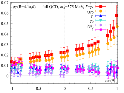
(a)

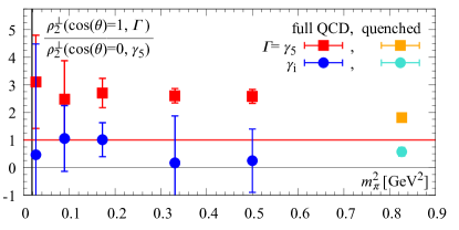
(b)

Figure 3: Diquark attractive effect. (Left) The density-density correlators $\rho_{2}^{\perp}(R=4.1a,\Theta,\Gamma)$ versus $cos(\Theta)$ at $m_{\pi}=575~{}\rm{MeV}$. (Right) The ratio $\rho_{2}^{\perp}(R,\Theta=0,\Gamma)/\rho_{2}^{\perp}(R,\Theta=\pi/2,\Gamma=\gamma_{5})$ versus $m_{\pi}^{2}$. Values above/below 1 for the red/blue points signal an attraction in the good diquark that is absent for the bad diquark. The vertical line denotes physical $m_{\pi}$.

The impact of the light-quark interactions on the spatial correlation between light quarks for different $\Gamma$ is displayed in Fig. 3 (left), which shows the density-density correlations $\rho_{2}^{\perp}(R,\Theta,\Gamma)$ as a function of $\cos(\Theta)$. For illustration, we show results for all $\Gamma$ at $R=4.1\,a$ for the ensemble with $m_{\pi}=575~{}\rm{MeV}$. As $\cos(\Theta)$ increases from $-1$ to $+1$, $r_{qq^{\prime}}$ decreases from $2R$ to $0$. The clear increase in $\rho_{2}$ seen in the good diquark channel is absent in all other channels renorm . The strengths of the quark-quark attractions in the good and bad diquark channels are further quantified in Fig. 3 (right), which shows the $m_{\pi}$ dependence of the ratios $\rho_{2}^{\perp}(R,\Theta=0,\Gamma)/\rho_{2}^{\perp}(R,\Theta=\pi/2,\Gamma=\gamma_{5})$ for $\Gamma=\gamma_{5}$ and $\gamma_{i}$. The ratio is $2$ or more for the good diquark across the whole range of $m_{\pi}$, but consistent with $0$ for the bad diquark, with no evidence for any $m_{\pi}$ dependence, apart from a possible low-$m_{\pi}$ enhancement for the good diquark. The results confirm a significant attractive quark-quark spatial correlation in the good diquark channel not present in the bad diquark channel, for all $m_{\pi}$ studied here.

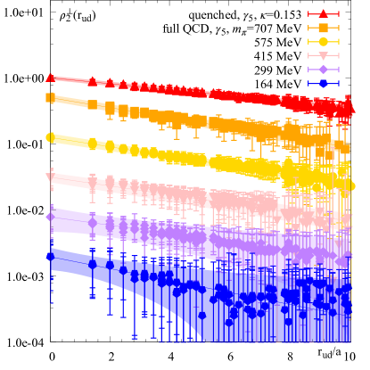
(a)

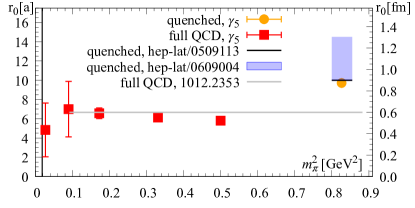
(b)

Figure 4: Good diquark size. (Left) Exponential decay with $r_{qq^{\prime}}$ of $\rho_{2}^{\perp}(R,\Theta)$. Each $m_{\pi}$ has its own color. Data sets have been normalised at $r_{qq^{\prime}}=0$ and offset vertically. Results for all available $R$ are shown together in one colored set. Each colored band comes from the combined fit used to determine the diquark size $r_{0}(m_{\pi}^{2})$. (Right) Resulting good diquark size $r_{0}$ versus $m_{\pi}^{2}$, compared to results of other lattice studies in the literature. The vertical line denotes physical $m_{\pi}$.

With a significant attractive good diquark spatial correlation established, we can refine our picture of the good diquark by studying its size and shape. We consider first the case $\phi=\pi/2$. At fixed $R$, $\rho_{2}^{\perp}(R,\Theta,\Gamma=\gamma_{5})$ depends only on $\Theta$ or, equivalently, $r_{qq^{\prime}}=R\sqrt{2(1-\cos(\Theta))}$. We find this dependence well represented by an exponential form, $\rho_{2}^{\perp}(R,r_{qq^{\prime}})\sim\exp(-r_{qq^{\prime}}/r_{0})$, for each value of $R$. As $R$ decreases and the diquark moves closer to the static quark, one might expect the latter to distort such diquark correlations and cause $r_{0}$ to vary. We see no evidence for such a variation, so long as $R>r_{qq^{\prime}}$, and thus, in the left panel of Fig. 4, display results for all $R$ together, for each $m_{\pi}$. We take $r_{0}$ as our definition of the good diquark size and fix its value from a combined fit to data for all such $R$. The resulting $r_{0}(m_{\pi}^{2})$ are displayed, and compared to those obtained in Refs. Alexandrou:2005zn ; Green:2010vc , in the right panel of Fig. 4. Recall that the parameters of our quenched ensemble match exactly those of Alexandrou:2005zn . Our results are in very good agreement with Alexandrou:2005zn , and with both the quenched and dynamical results of Green:2010vc .

Increasing $m_{q_{1,2}}$ should, on its own, produce a more compact object. The accompanying decrease in good diquark attraction seen in Tab. 1 will, however, work in the opposite direction. We see some evidence that the former effect dominates for larger $m_{\pi}$ (above $\sim 400$ MeV) though, in the limit of infinitely massive sea quarks (i.e. the quenched case) the diquarks are definitely larger. As Fig. 4 (right) indicates, in full QCD, over a range of $m_{\pi}$, $r_{0}$ is of the order of $0.6~{}\rm{fm}$, a size similar to that of static-light mesons when measured the same way Blossier:2016vgh . This result is also in good agreement with that of a phenomenological, relativistic quark-diquark model study of nucleon form factors DeSanctis:2011zz , which found a fitted $0^{+}$ diquark form factor corresponding to an rms diquark size of $\sim 0.54$ fm. It should be noted that the determined diquark size does not affect the spectroscopy of models that include diquarks as effective degrees of freedom. Our results clearly support diquark modelling of the baryon structure which allows for the possibility of a non-zero diquark size.

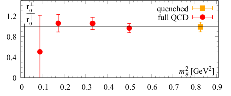
(a)

Figure 5: Good diquark shape. The ratio $r_{0}^{\perp}/r_{0}^{\parallel}$ as a function of $m_{\pi}$. The vertical line denotes physical $m_{\pi}$.

Finally, we can learn about the good diquark shape, by comparing the density-density correlation falloff for the relative radial ($\phi=\pi$) and tangential ($\phi=\pi/2$) orientations of $\vec{x}_{2}-\vec{x}_{1}$ and $\vec{S}$ (sketched in Fig. 7 of App. D). We define separate radial (${\parallel}$) and tangential ($\perp$) size parameters, $r_{0}^{\parallel}$ and $r_{0}^{\perp}$, from exponential fits to the data for $\rho_{2}^{\perp}(R,\Theta)$ and $\rho_{2}^{\parallel}\,(r_{qq^{\prime}},S)$, detailed in App. D and shown in the left and right panels of Fig. 8.

The ratio $r_{0}^{\perp}/r_{0}^{\parallel}$ provides a measure of whether the diquarks are prolate, oblate, or neither. The results are shown in Fig. 5. We find $r_{0}^{\perp}/r_{0}^{\parallel}(m_{\pi}^{2})\simeq 1$ within errors for all $m_{\pi}$, indicating that the diquarks have a near-spherical shape. This is consistent with the scalar, $J=0$ nature of the good diquark, though the presence of the static quark could, in principle, have induced a diquark polarization. There appears no need to include a dipole term in diquark models.

4 Summary and conclusions

Using a gauge-invariant setup, we have studied the masses and shapes of diquarks carrying different quantum numbers. Our study is the first to consider $n_{f}=2+1$ flavors of dynamical quarks with a range of $u,d$ masses corresponding to $m_{\pi}$ as low as $164~{}\rm{MeV}$. This allows for a small, controlled extrapolation to physical $m_{\pi}\approx 135~{}\rm{MeV}$. The resulting diquark mass differences presented in Fig. 1 and Tab. 1 confirm the special status of the “good” diquark channel, which shows an attraction of $198(4)~{}\rm{MeV}$ over the “bad” channel, more over the others. A simple interpolation Ansatz Eq. (2) accurately describes how this attraction varies with $m_{\pi}$, and with the diquark flavor composition. Extrapolation of our results to the continuum limit is still required, but this has been found to amount to a small correction, at the percent level, in other hadronic mass measurements on the same gauge configurations Padmanath:2019ybu ; Namekawa:2013vu ; Alexandrou:2017xwd ; Hudspith:2017bbh . We have also measured the mass difference between a good diquark and an [anti]quark, as per Tab. 1.

We have also shown that the $q-q$ attraction responsible for the bad-good diquark mass differences induces a compact spatial correlation, present in the “good” diquark channel only. The associated “good” diquark size, extracted from the spatial decay rate of quark density-density correlations, is ${\cal O}(0.6)$ fm, similar to that of ordinary mesons and baryons Blossier:2016vgh , and varies little with light-quark mass.

Finally, we have tried to refine the diquark picture further, by studying the shape of quark density-density correlations in a good diquark, in the background of a heavy, static quark. It turns out that good diquarks are nearly spherical, with no signal within errors of a departure from this simplest shape.

The information obtained above may prove useful, both in identifying channels favorable to the existence of low-lying tetraquark or pentaquark states, and in obtaining rough estimates of their expected masses. Such qualitative guidance has, in fact, already been exploited in identifying double-open-heavy-flavor, $SU(3)_{F}$ flavor $\bar{3}_{F}$, $J^{P}=1^{+}$ $\bar{Q}\bar{Q}^{\prime}qq^{\prime}$ channels as favorable to the existence of exotic tetraquark states. In such channels, a localized four-quark configuration benefits from the attractive good-light-diquark and color $3_{c}$ heavy-antidiquark Coulomb interactions, neither of which is accessible for two well-separated heavy-light mesons. This observation motivated both phenomenological and lattice explorations of potential binding in such doubly heavy tetraquark channels, and experimental searches for bound doubly heavy tetraquark states, the latter culminating in the LHCb discovery of the exotic doubly charmed $T_{cc}$ tetraquark state LHCb:2021vvq ; LHCb:2021auc . Multiple recent lattice studies using interpolating operators designed to access the expected good-light-diquark configuration now also provide clear evidence for the existence of a $J^{P}=1^{+}$, $SU(3)_{F}$ $\bar{3}_{F}$ multiplet of doubly bottom strong-interaction-stable tetraquark states Francis:2016hui ; Bicudo:2015kna ; Bicudo:2012qt ; Bicudo:2016ooe ; Junnarkar:2018twb ; Leskovec:2019ioa ; Hudspith:2020tdf ; Mohanta:2020eed ; Bicudo:2021qxj . An analogous qualitative diquark-based argument identifies the singly-heavy $J^{P}=1/2^{+}$, $I=1/2$, $\bar{Q}sudd$ channel as one potentially favorable to the existence of an exotic pentaquark resonance. Explicitly, while at most one good light diquark can exist in a state consisting of a well-separated heavy-light meson and light-quark baryon, a localized singly heavy five-quark state can contain two good light diquarks, one non-strange and one strange. The possibility that the short-distance part of the associated singly heavy meson-light baryon system might have an attractive component resulting from this localized ”extra-good-light-diquark” configuration motivates further study of this channel. Outstanding issues still to be investigated are potential distortions of the good diquark correlation caused by the presence of additional light quarks and/or the impact of Pauli blocking in channels, like this, where more than one good light diquark may be present. These are questions that might be amenable to investigation using microscopic models which survive the tests of predicting very shallow binding in the $T_{cc}$ channel and binding energies compatible with now well-established lattice results for the non-strange and strange doubly bottom $J^{P}=1^{+}$, $\bar{3}_{F}$ channels. Bound or resonant singly-heavy $J^{P}=1/2^{+}$, $I=1/2$, $\bar{Q}sudd$ pentaquark states, if they exist, would have four open flavors and hence, like the doubly heavy tetraquarks, be manifestly exotic.

Our three sets of results – bad-good diquark mass difference, good diquark size and shape – paint a diquark picture entirely consistent with that used in diquark models and provide clear, quantitative support for the good diquark picture. Diquark models are playing an important role in explorations of possible multi-quark exotics, especially in channels too complex to permit a complete theoretical analysis. In such channels, various light quark pairings into compact good diquark composites are likely to occur, especially when heavy $c,b$ quark sources are present (see e.g. Karliner:2017qjm ; Eichten:2017ffp ; Czarnecki:2017vco for phenomenological and Wagner:2011ev ; Brown:2012tm ; Bicudo:2015kna ; Bicudo:2012qt ; Bicudo:2015vta ; Bicudo:2016ooe ; Francis:2016hui ; Francis:2018jyb ; Junnarkar:2018twb ; Leskovec:2019ioa ; Hudspith:2020tdf ; Mohanta:2020eed ; Bicudo:2021qxj for lattice studies). Which pairing is energetically favored depends sensitively on the numerical values of the parameters of the diquark model. Our study may sharpen these values, and help improve the reliability of such diquark analyses.

Appendix A Phenomenological Expectations

Ref. Jaffe:2004ph discussed in detail how to obtain phenomenological estimates for the static-limit values of the bad-good diquark and diquark-antiquark mass differences using combinations of single-charm and single-bottom meson and baryon masses chosen so $O(1/m_{Q})$ contributions cancel, bringing the results closer to the static limit. Comparing the estimates for a given splitting obtained using charm input to that obtained using bottom input provides an assessment of how close to the static limit the bottom-based estimate is likely to be. This data-based approach is obviously very closely related to the gauge-invariant, static limit approach used to obtain our lattice results above. In this appendix we provide an update of the numerical analysis of Ref. Jaffe:2004ph . We also remind the reader of a number of other, generally more model-dependent approaches, that have been used to obtain estimates of the good-bad diquark splittings.

Ref. Jaffe:2004ph gives expressions for the combinations needed to provide phenomenological estimates for four of the splittings we have measured. Explicitly, the combination

$$\frac{1}{3}\left(2M(\Sigma^{*}_{Q})+M(\Sigma_{Q})\right)-M(\Lambda_{Q})$$ (6)

provides an estimate for $\delta(1^{+}-0^{+})_{ud}$, the combination

$$\frac{2}{3}\left(M(\Xi^{*}_{Q})+M(\Sigma_{Q})+M(\Omega_{Q})\right)-M(\Xi_{Q})-M(\Xi^{\prime}_{Q})$$ (7)

an estimate for $\delta(1^{+}-0^{+})_{us}$, the combination

$$M(\Lambda_{Q})-\frac{1}{4}\left(M(P_{Qu})+3M(V_{Qu})\right)\,,$$ (8)

with $P_{Qu}$ and $V_{Qu}$ the ground-state, heavy-light pseudoscalar and vector mesons, an estimate for $\delta(Q[ud]_{0^{+}}-\bar{Q}u)$, and the combination

$$M(\Xi_{Q})+M(\Xi^{\prime}_{Q})-\frac{1}{2}(M(\Sigma_{Q})+M(\Omega_{Q}))$$

$$\qquad\qquad-\frac{1}{4}(M(P_{Qs})+3M(V_{Qs}))\,,$$ (9)

with $P_{Qs}$ and $V_{Qs}$ the ground-state, heavy-strange pseudoscalar and vector mesons, an estimate for $\delta(Q[us]_{0^{+}}-\bar{Q}s)$. For a given static-limit splitting, the most accurate estimate should be that obtained using bottom hadron input, while the difference between the charm- and bottom-based estimates should provide a conservative assessment of the deviation of the bottom-based estimate from the actual static-limit value. At the time Ref. Jaffe:2004ph was written, information on bottom hadron masses was limited, and only one of these four splittings, $\delta(Q[ud]_{0^{+}}-\bar{Q}u)$, could be estimated with both charm and bottom input. The agreement between the two was excellent. It is now possible to estimate all four splittings using both charm and bottom input. Using PDG 2021 input Zyla:2020zbs , we find, for $\delta(1^{+}-0^{+})_{ud}$, $210$ MeV using charm input and $206$ MeV using bottom input; for $\delta(1^{+}-0^{+})_{us}$, $148$ MeV using charm input and $145$ MeV using bottom input; for $\delta(Q[ud]_{0^{+}}-\bar{Q}u)$, $313$ MeV using charm input and $306$ MeV using bottom input; and, for $\delta(Q[us]_{0^{+}}-\bar{Q}s)$ $398$ MeV using charm input and $397$ MeV using bottom input. It follows that the bottom-based phenomenological estimates for the static-limit splittings should be reliable to $O(7)\ {\rm MeV}$ or better. Moreover, these estimates agree well with the results shown in Tab. 1.

A number of other approaches have also been used to estimate the $ud$ and $\ell s$ good-bad diquark splittings.

In the Dyson-Schwinger equation (DSE) approach, earlier analyses employing the rainbow-ladder approximation obtained $\delta(1^{+}-0^{+})_{ud}=212$ MeV and $\delta(1^{+}-0^{+})_{us}=168$ MeV Burden:1996nh , $\delta(1^{+}-0^{+})_{ud}=202$ MeV Maris:2005zy , $\delta(1^{+}-0^{+})_{ud}=270(30)$ MeV Eichmann:2008ef , $\delta(1^{+}-0^{+})_{ud}=280$ MeV Roberts:2011cf . A more recent analysis, Ref. Eichmann:2016hgl , reports a result $\delta(1^{+}-0^{+})_{ud}=190(20)$ MeV, in good agreement with both our lattice determination and the updated version of the phenomenological estimate of Ref. Jaffe:2004ph .

The good-bad diquark mass splittings have also been obtained from diquark-quark model analyses of the non-strange and strange baryon spectrum in which the diquark mass enters as a free parameter of the model and is obtained as part of the fit to the spectrum. An iterative, phenomenological version of this approach Lichtenberg:1996fi produced the results $\delta(1^{+}-0^{+})_{ud}=205$ MeV and $\delta(1^{+}-0^{+})_{us}=140$ MeV, while a more microscopic, relativistic model, which did not, however, allow for the possibility of mixing between quark-scalar-diquark and quark-axial-vector-diquark configurations, obtained a larger result, $\delta(1^{+}-0^{+})_{ud}=350$ MeV, for the $ud$ diquark splitting Ferretti:2011zz . A modified version of this model, which significantly improves the quality of the model fit to known $3^{*}$ and $4^{*}$ baryon resonances, obtained by adding a term to the effective interaction that allows such mixing to occur, in contrast, produces a result $\delta(1^{+}-0^{+})_{ud}=210$ MeV in good agreement with both our lattice determination and the updated version of the phenomenological estimate of Ref. Jaffe:2004ph .

An alternate implementation of the microscopic quark-diquark model approach first fits the parameters of a model two-body quark-antiquark effective interaction with one-gluon-exchange color dependence, $F_{q}\cdot F_{\bar{q}}$, to the meson spectrum, then uses this interaction, with $F_{q}\cdot F_{\bar{q}}$ replaced by the corresponding quark-quark one-gluon-exchange factor, $F_{q}\cdot F_{q}$, to determine the nominal $\bar{3}_{c}$, $J^{P}=0^{+}$ and $1^{+}$ masses, and hence the $1^{+}$-$0^{+}$ splittings. The meson sector model used in Ref. Ebert:2011kk (which has a two-body confinement interaction involving a linear combination of scalar and vector structures) produces the results $\delta(1^{+}-0^{+})_{ud}=199$ MeV and $\delta(1^{+}-0^{+})_{us}=121$ MeV Ebert:2011kk , while the Godfrey-Isgur model Godfrey:1985xj used in Ref. Ferretti:2019zyh (with its purely scalar two-body confinement form) produces the results $\delta(1^{+}-0^{+})_{ud}=149$ MeV and $\delta(1^{+}-0^{+})_{us}=106$ MeV.

In view of the good agreement between the updated versions of the charm- and bottom-based estimates of Ref. Jaffe:2004ph , we consider the bottom-based results to represent the best phenomenological estimates of the gauge-invariant static limit splittings we measure on the lattice. The other approaches, which are more model-dependent, but have the advantage of being applicable to non-strange and strange baryon sector, produce results in reasonable to good agreement with the heavy-quark based phenomenological estimates for the good-bad diquark splittings, with more recent versions of the analyses typically producing improved agreement. It is, of course, possible that the additional light quarks present in non-strange and strange baryons might affect the structure of the good light diquark correlation in those systems, causing it to differ from that found in singly heavy baryon systems. The agreement of the results for the diquark splittings obtained from (albeit model-dependent) analyses of the light baryon sector with the heavy-quark-based phenomenological estimates is thus of interest since it supports the picture in which the same good light diquark correlations serve as useful effective degrees of the freedom in light and heavy baryon sectors.

Appendix B Lattice ensembles and propagators

For the numerical studies, we re-use the set of propagators from Francis:2016hui ; Francis:2018jyb determined on the publicly available $n_{f}=2+1$ flavor full QCD gauge ensembles provided by the PACS-CS’09 collaboration Aoki:2008sm ; Namekawa:2013vu via the JLDG repository JLDG . The quoted values of $m_{\pi}$ and lattice spacing originate from our own previous re-determination Hudspith:2017bbh ; Francis:2016nmj . These gauge configurations have been used extensively within the lattice community. A known caveat is the slight mistuning of the strange sea quark mass Aoki:2008sm . The value of the hopping parameter which produces the physical strange quark mass is, however, known, and we set the strange valence quark mass to this value, thus introducing a tiny amount of partial quenching.

To connect with previous studies in the quenched setup discussed in Alexandrou:2006cq , and in more detail in Alexandrou:2005zn , we generated a new ensemble with the same lattice parameters, in particular with coupling $\beta=6.0$ and hopping parameter $\kappa=0.153$ for propagator inversions. This corresponds to a valence pion mass $m_{\pi}^{v}=909\,\rm{MeV}$.

All propagators were computed using the deflated SAP-GCR solver CLScode and have Coulomb gauge-fixed wall sources, where the gauge was fixed using the FACG-algorithm in the implementation of Hudspith:2014oja ; GLUcode .

We can re-use the propagators without further inversions since the gauge-fixed wall sources enable the contraction of the density correlators without an additional sequential source propagator. Choosing $(t_{snk}-t_{src})=16$ enables us to perform multiple measurements on each configuration. Setting $t_{m}$ midway between source and sink minimizes excited-state contamination.

For the static quark we compute propagators on the fly via ($t_{2}>t_{1}$)DellaMorte:2005nwx :

$$S(\bm{x},t_{2},\bm{x},t_{1})=\Big{(}\frac{1+\gamma_{0}}{2}\Big{)}\Big{[}\prod_{t=t_{1}}^{t_{2}-a}U_{0}(\bm{x},t)\Big{]}$$ (10)

where we dropped the exponential prefactor, since it amounts to a constant shift in the masses that either drops out in the difference or is irrelevant to the results. To reduce statistical fluctuations, the gauge links are smeared using HYP smearing (type 1 Donnellan:2010mx ; Hasenfratz:2001hp ) in all 4 dimensions, which introduces some non-locality in time. In all cases we made sure that the propagation time $t$ is large enough and the number of smearing steps small enough to ensure negligible effects aside from the boosted signal. Furthermore we considered several smearing setups and smearing radii. We observed comparable results and selected the one giving the best signal-to-noise properties. Our lattice parameters are listed in Tab. 2.

Label	$L\times T$	$a^{-1}[\rm{GeV}]$	$m_{\pi}[\rm{MeV}]$	$n_{cfg}$	$n_{meas}^{spec}$	$n_{meas}^{struct}$
Q	$32\times 64$	$2.15$	909	374	374	374
E1	$32\times 64$	$2.194$	707	399	1596	798
E2	”	”	575	400	1600	800
E4	”	”	415	400	3200	2800
E5	”	”	299	800	6400	5600
E6	”	”	164	198	6336	2574

Table 2: Parameters of the lattice calculation. $n_{meas}^{spec}$ and $n_{meas}^{struct}$ indicate how many measurements in total were made of the baryon/meson correlators for the spectroscopy study, and of the density-density correlators for the structure analysis, respectively. For the latter analysis, the sink-source time propagation is set to $(t_{snk}-t_{src})=16$, with the currents inserted at $t_{m}=8$, see also the sketch in Fig. 2 (left).

Appendix C Lattice spectroscopy analysis details

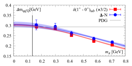
Figure 6: Agreement of the bad-good diquark mass splitting with the prediction Jaffe:2004ph , $\delta(\Delta-N)=3/2\times\delta(1^{+}-0^{+})_{ud}$.

To study the mass differences between good and bad diquarks, shown in top and middle panels of Fig. 1, we fix the energies in the following way: First, we analyze the smeared and unsmeared correlators separately. For each dataset, we consider one- and two-state fits. The fit window in Euclidean time is the longest for which both fits give ground-state energies consistent within errors. The ground-state energies of the smeared and unsmeared data sets are then averaged, and the larger of the two uncertainties assigned as the final error.

When performing the extrapolations to physical $m_{\pi}$, we also considered combined fits with the Ansatz Eq. (2) using free $n$ and shared $B$, but did not find an improvement and therefore quote results from individual fits. As a further consistency check note that all three extrapolations intersect for large $m_{\pi}$ at the $n_{f}=3$ flavor-symmetric point without having enforced this expectation through a shared parameter.

In the bottom panel of Fig. 1 we show the difference in mass between single-static octet baryons and static-light pseudoscalar mesons, as explained in the text. In this data the excited state contamination is much larger and we extract the masses by fitting both smeared and unsmeared data with a two-state Ansatz. As before we take the values from the longest time interval where the fitted ground states agree within errors, average the results, and quote the larger of the two uncertainties as our error. For the $ud-u$, $\ell s-s$ and $\ell s-\ell$ cases we observe the expected $n_{f}=3$ degeneracy as $m_{u,d}\rightarrow m_{s}$.

As a final diquark spectroscopy investigation, we compare the bad-good diquark mass difference with the $\Delta$-$N$ mass splitting for each of our 5 ensembles. This comparison is motivated by the observation Jaffe:2004ph that, in the one-gluon-exchange approximation, and chiral limit, $\delta(\Delta-N)=\frac{3}{2}\delta(1^{+}-0^{+})$. Fig. 6 compares the left- and right-hand sides of this relation, the red curve showing the appropriately rescaled version of the $\delta(1^{+}-0^{+})_{ud}$ fit of the middle panel of Fig. 1 and the blue curve a similar fit to the $\Delta$-$N$ data with $A=\frac{3}{2}\times 0.203(9),~{}B=1.10(11)$ GeV. Agreement between the two is excellent in the chiral limit, and remains very good over the whole mass range. Measurements of the $\Delta-N$ splitting were newly performed for this study, using the same propagators as for the static baryons shown so far. Since in this case we do not benefit from the cancellation of the heavy quark mass, and nucleon correlators generally suffer from the well known signal-to-noise problem, we expect larger uncertainties in this study. The situation is further complicated as the $\Delta$ baryon is a resonance in nature: a single operator analysis, as performed here, can capture only its rough features. To stabilise the extraction of the masses here, we fitted the channel pairs $\Gamma=(\gamma_{i},\sigma_{i0})$ and $(\gamma_{5},\gamma_{5}\gamma_{0})$ simultaneously with single exponentials and chose to quote the parameters from the longest combined plateau. For the physical-point extrapolation, the results were fitted to the same Ansatz Eq. (2), in the same way as before.

Appendix D Lattice structure analysis details

The diquark size $r_{0}$ can be estimated from the fitted rate of the exponential decay, $\sim\exp(-r_{qq^{\prime}}/r_{0})$, of the density-density correlator $\rho_{2}^{\perp}(R,r_{qq^{\prime}})$, with $r_{qq^{\prime}}$ the distance between the two current insertion points: see Fig. 4 (left).

The colored bands (one for each $m_{\pi}$) are the result of performing a combined fit for all available $R$ to a single exponential with shared size parameter $r_{0}$ and separate amplitudes. Note that our lattice spatial size is about $5r_{0}$, so we neglect corrections caused by periodic boundary conditions which were studied in Green:2010vc . We checked the dependence of $r_{0}(R)$ on $R$ through individual fits and found no significant dependence for $R\in[3:6]$. Similar findings were reported in Alexandrou:2005zn . Of course, if $R$ is increased beyond $\sim 1\,\rm{fm}$, the effective string between the static quark and the diquark will break and a light baryon will form, with qualitatively different diquark correlations. Our study does not consider this large-distance regime. Also, for a given $R$, we normally would quote the number from the largest stable fit window. However, due to our chosen geometry we may expect interference from the static quark when $r_{qq^{\prime}}\gtrsim R$, and we limit the fit window accordingly.

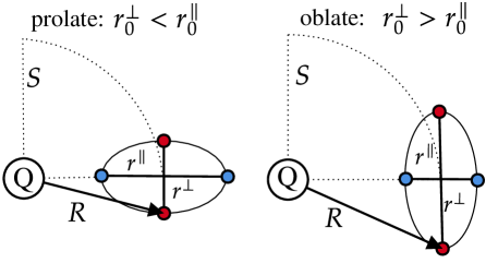
Figure 7: Diquark shape: 2D sketch of the 2 current insertions. Comparing exponential fall-offs in the $\perp$ and $\parallel$ directions gives a measure of the diquark shape: prolate (left) or oblate (right).

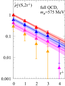
(a)

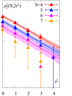
(b)

Figure 8: Good diquark shape. $m_{\pi}=575$ MeV results for the $r_{qq^{\prime}}$-dependence of $\rho_{2}(r_{qq^{\prime}},S,\phi)$ for tangential ($\phi=\pi/2$, left panel) and radial ($\phi=\pi$, right panel) quark-quark orientations. The colored error bands are the results of combined fits to data for each of $S=4a$, $5a$ and $6a$.

Separate sizes $r_{0}^{\perp}$ and $r_{0}^{\parallel}$ can be defined for the tangential and radial geometries shown in Fig. 7. The ratio of sizes $r_{0}^{\perp}/r_{0}^{\parallel}$ then gives a measure of whether the diquarks are spherical ($r_{0}^{\perp}/r_{0}^{\parallel}=1$), prolate ($r_{0}^{\perp}/r_{0}^{\parallel}<1$), or oblate ($r_{0}^{\perp}/r_{0}^{\parallel}>1$).

To estimate $r_{0}^{\perp}$ and $r_{0}^{\parallel}$, we measure $\rho_{2}(r_{qq^{\prime}},S,\phi)$ for the two geometries of Fig. 7, with $r_{0}^{\perp}$ and $r_{0}^{\parallel}$ corresponding to $\phi=\pi/2$ and $\pi$ in Fig. 2, respectively. When the line labelled $S$ in Fig. 2 points along the $x$ axis, the current insertion points for the radial configuration (the blue points in Fig. 7) are ${x}_{1,2}=(S\pm r^{\parallel},0,0)$, while those for the tangential configuration (the red points in Fig. 7) are ${x}_{1,2}=(S,\pm r^{\perp},0)$. For simplicity, we take the line labelled $S$ to always lie in one of the $x$, $y$ or $z$ axis directions, considering all such permutations.

Focusing first on the radial case, $x_{1}+x_{2}=2S$ is constant at fixed $S$ and independent of $r^{\parallel}$. Here we define our radial size parameter, $r_{0}^{\parallel}$, at this fixed $S$, by fitting the $r^{\parallel}$ dependence to the form

$$\rho_{2}^{\parallel}(S,r^{\parallel})\sim\exp(-r^{\parallel}/r_{0}^{\parallel})~{}~{}.$$ (11)

Since no obvious $S$ dependence is observed, we arrive at $r_{0}^{\parallel}$ by analyzing the data in a combined fit for several $S$ using the same fit method applied before.

In the tangential case, a complication arises. Our previously introduced size parameter, $r_{0}$, was defined through a fit to $\rho_{2}^{\perp}(R,r^{\perp})$ with variable $r^{\perp}$, but fixed $R$. Since, however, $R=\sqrt{(r^{\perp})^{2}+S^{2}}$, when $r^{\perp}$ varies at fixed $R$, $S$ also varies. This is not the fixed-$S$ situation used to define $r_{0}^{\parallel}$. We thus need to define an alternate tangential size parameter, $r_{0}^{\perp}$, through a fit to data with variable $r^{\perp}$ but fixed $S$, in order to compare tangential and radial size parameters both defined at fixed $S$. As seen above, the density-density correlation $\rho_{2}^{\perp}(R,r^{\perp})$ at fixed $r^{\perp}$ varies with $R$. We find this dependence well described by an exponential form $\sim\exp(-2R/R_{0})$. The dependence of the density-density correlation on $r^{\perp}$ at fixed $S$ in the tangential configuration can then be obtained by fitting the product $\rho_{2}^{\perp}(R,r^{\perp})\exp(+2R/R_{0})$, evaluated at fixed $S$ and variable $r^{\perp}$, to the form $\exp(-r^{\perp}/r_{0}^{\perp})$. Since the fixed-$S$ tangential $r^{\perp}=0$ and radial $r^{\parallel}=0$ configurations are geometrically degenerate, it is convenient to instead use the form $\exp(-r^{\perp}/r_{0}^{\perp})$ to fit the modified product

$$\hat{\rho}_{2}^{\perp}(S,2r^{\perp})=\rho_{2}(R,2r^{\perp})\,\exp(+\frac{2R}{R_{0}})\,\exp(-\frac{2S}{R_{0}})\,,$$ (12)

with $R_{0}$ a second fit parameter, and the right-hand side evaluated at fixed $S$. The extra $r^{\perp}$-independent factor, $\exp(-2S/R_{0})$, ensures that, in the limit that $r^{\perp}\rightarrow 0$ and hence $R\rightarrow S$, the quantity being fit reduces to $\rho_{2}^{\perp}(R=S,r^{\perp}=0)$. Since this is identical to the analogous zero-separation quantity, $\rho_{2}^{\parallel}(S,r^{\parallel}=0)$, which enters the fit used to determine $r_{0}^{\parallel}$, this choice ensures a common normalization for the tangential and radial fits, at the $r^{\perp}=r^{\parallel}=0$ point common to both.

In the left and right panels of Fig. 8 we show, for the $m_{\pi}=575~{}\rm{MeV}$ ensemble and $S$ ranging from $4$ to $7$ times the lattice spacing, the dependences of $\hat{\rho}_{2}^{\perp}(S,2r^{\perp})$ on $r^{\perp}$ and $\rho_{2}^{\parallel}(S,2r^{\parallel})$ on $r^{\parallel}$, respectively. The results are normalized so $\hat{\rho}_{2}^{\perp}(S,2r^{\perp})$ and $\rho_{2}^{\parallel}(S,2r^{\parallel})$ take the common value $1$ at $S=4a$ and zero separation.

While the parameters $r_{0}^{\perp}$ and $R_{0}$ have been determined in the two-parameter fit described above, $R_{0}$ could, in principle, also be determined by fitting $\rho_{2}^{\perp}(R,r^{\perp})$, with $r^{\perp}$ fixed to zero, to the form $\sim\exp(-2R/R_{0})$. We found that inserting the resulting $R_{0}$ into the Ansatz Eq. (12) and subsequently fitting $r_{0}^{\perp}$ produced no improvement over the direct two-parameter fit result, once errors were propagated and correlations taken into account.

In both the radial and tangential cases, we have propagated all errors within a bootstrap procedure, which allows us to also evaluate the uncertainty on the ratio $r_{0}^{\perp}/r_{0}^{\parallel}$ consistently. Results for this ratio are shown as a function of $m_{\pi}^{2}$ in Fig. 5 of the main text. We observe that the errors on the data limit the precision of the analysis, with a stable result, for example, not even attainable for the $m_{\pi}=164~{}\rm{MeV}$ ensemble. This is due in part to the noisiness of the results at large $S$, which were not precise enough to constrain $R_{0}$, $r_{0}^{\perp}$ and $r_{0}^{\parallel}$ further.

References

- (1) R. Jaffe, Exotica, Phys. Rept. 409 (2005) 1 [hep-ph/0409065].
- (2) A. Ali, J.S. Lange and S. Stone, Exotics: Heavy Pentaquarks and Tetraquarks, Prog. Part. Nucl. Phys. 97 (2017) 123 [1706.00610].
- (3) M. Barabanov et al., Diquark Correlations in Hadron Physics: Origin, Impact and Evidence, 2008.07630.
- (4) M. Gell-Mann, A Schematic Model of Baryons and Mesons, Phys. Lett. 8 (1964) 214.
- (5) M. Ida and R. Kobayashi, Baryon resonances in a quark model, Prog. Theor. Phys. 36 (1966) 846.
- (6) D.B. Lichtenberg, W. Namgung, E. Predazzi and J.G. Wills, Baryon Masses in a Relativistic Quark - Diquark Model, Phys. Rev. Lett. 48 (1982) 1653.
- (7) R.T. Cahill, C.D. Roberts and J. Praschifka, Calculation of Diquark Masses in QCD, Phys. Rev. D36 (1987) 2804.
- (8) P. Maris, Effective masses of diquarks, Few Body Syst. 32 (2002) 41 [nucl-th/0204020].
- (9) E. Santopinto, An Interacting quark-diquark model of baryons, Phys. Rev. C72 (2005) 022201 [hep-ph/0412319].
- (10) A. De Rujula, H. Georgi and S.L. Glashow, Hadron Masses in a Gauge Theory, Phys. Rev. D12 (1975) 147.
- (11) T.A. DeGrand, R.L. Jaffe, K. Johnson and J.E. Kiskis, Masses and Other Parameters of the Light Hadrons, Phys. Rev. D12 (1975) 2060.
- (12) G. ’t Hooft, Computation of the Quantum Effects Due to a Four-Dimensional Pseudoparticle, Phys. Rev. D14 (1976) 3432.
- (13) E.V. Shuryak, The Role of Instantons in Quantum Chromodynamics. 1. Physical Vacuum, Nucl. Phys. B203 (1982) 93.
- (14) T. Schäfer and E.V. Shuryak, Instantons in QCD, Rev. Mod. Phys. 70 (1998) 323 [hep-ph/9610451].
- (15) M. Hess, F. Karsch, E. Laermann and I. Wetzorke, Diquark masses from lattice QCD, Phys. Rev. D58 (1998) 111502 [hep-lat/9804023].
- (16) Y. Bi, H. Cai, Y. Chen, M. Gong, Z. Liu, H.-X. Qiao et al., Diquark mass differences from unquenched lattice QCD, Chin. Phys. C 40 (2016) 073106 [1510.07354].
- (17) R. Babich, N. Garron, C. Hoelbling, J. Howard, L. Lellouch and C. Rebbi, Diquark correlations in baryons on the lattice with overlap quarks, Phys. Rev. D76 (2007) 074021 [hep-lat/0701023].
- (18) K.B. Teo and J.W. Negele, The Definition and lattice measurement of hadron wave functions, Nucl. Phys. Proc. Suppl. 34 (1994) 390.
- (19) J.W. Negele, Hadron structure in lattice QCD: Exploring the gluon wave functional, in Excited nucleons and hadronic structure. Proceedings, Conference, NSTAR 2000, Newport News, USA, February 16-19, 2000, pp. 368–377, 2000 [hep-lat/0007026].
- (20) C. Alexandrou, P. de Forcrand and A. Tsapalis, Probing hadron wave functions in lattice QCD, Phys. Rev. D66 (2002) 094503 [hep-lat/0206026].
- (21) K. Orginos, Diquark properties from lattice QCD, PoS LAT2005 (2006) 054 [hep-lat/0510082].
- (22) C. Alexandrou, P. de Forcrand and B. Lucini, Searching for diquarks in hadrons, PoS LAT2005 (2006) 053 [hep-lat/0509113].
- (23) C. Alexandrou, P. de Forcrand and B. Lucini, Evidence for diquarks in lattice QCD, Phys. Rev. Lett. 97 (2006) 222002 [hep-lat/0609004].
- (24) J. Green, J. Negele, M. Engelhardt and P. Varilly, Spatial diquark correlations in a hadron, PoS LATTICE2010 (2010) 140 [1012.2353].
- (25) J. Green, M. Engelhardt, J. Negele and P. Varilly, Diquark correlations in a hadron from lattice QCD, AIP Conf. Proc. 1441 (2012) 172.
- (26) R. Fukuda and P. de Forcrand, Searching for evidence of diquark states using lattice QCD simulations, PoS LATTICE2016 (2017) 121.
- (27) PACS-CS collaboration, 2+1 Flavor Lattice QCD toward the Physical Point, Phys. Rev. D 79 (2009) 034503 [0807.1661].
- (28) PACS-CS collaboration, Charmed baryons at the physical point in 2+1 flavor lattice QCD, Phys. Rev. D 87 (2013) 094512 [1301.4743].
- (29) https://www.jldg.org.
- (30) A. Francis, R.J. Hudspith, R. Lewis and K. Maltman, Lattice Prediction for Deeply Bound Doubly Heavy Tetraquarks, Phys. Rev. Lett. 118 (2017) 142001 [1607.05214].
- (31) A. Francis, R.J. Hudspith, R. Lewis and K. Maltman, Evidence for charm-bottom tetraquarks and the mass dependence of heavy-light tetraquark states from lattice QCD, Phys. Rev. D 99 (2019) 054505 [1810.10550].
- (32) M. Della Morte, A. Shindler and R. Sommer, On lattice actions for static quarks, JHEP 08 (2005) 051 [hep-lat/0506008].
- (33) M. Donnellan, F. Knechtli, B. Leder and R. Sommer, Determination of the Static Potential with Dynamical Fermions, Nucl. Phys. B 849 (2011) 45 [1012.3037].
- (34) The slight difference in the two results originates from their two different renormalisation constants. Unfortunately these are not available for the ensembles studied.
- (35) B. Blossier and A. Gérardin, Density distributions in the meson, Phys. Rev. D 94 (2016) 074504 [1604.02891].
- (36) M. De Sanctis, J. Ferretti, E. Santopinto and A. Vassallo, Electromagnetic form factors in the relativistic interacting quark-diquark model of baryons, Phys. Rev. C 84 (2011) 055201.
- (37) M. Padmanath, Heavy baryon spectroscopy from lattice QCD, 1905.10168.
- (38) C. Alexandrou and C. Kallidonis, Low-lying baryon masses using twisted mass clover-improved fermions directly at the physical pion mass, Phys. Rev. D 96 (2017) 034511 [1704.02647].
- (39) R.J. Hudspith, A. Francis, R. Lewis and K. Maltman, Heavy and light spectroscopy near the physical point, Part I: Charm and bottom baryons, PoS LATTICE2016 (2017) 133.
- (40) M. Karliner and J.L. Rosner, Discovery of doubly-charmed baryon implies a stable () tetraquark, Phys. Rev. Lett. 119 (2017) 202001 [1707.07666].
- (41) E.J. Eichten and C. Quigg, Heavy-quark symmetry implies stable heavy tetraquark mesons , Phys. Rev. Lett. 119 (2017) 202002 [1707.09575].
- (42) A. Czarnecki, B. Leng and M.B. Voloshin, Stability of tetrons, Phys. Lett. B 778 (2018) 233 [1708.04594].
- (43) ETM collaboration, Static-static-light-light tetraquarks in lattice QCD, Acta Phys. Polon. Supp. 4 (2011) 747 [1103.5147].
- (44) Z.S. Brown and K. Orginos, Tetraquark bound states in the heavy-light heavy-light system, Phys. Rev. D 86 (2012) 114506 [1210.1953].
- (45) P. Bicudo, K. Cichy, A. Peters and M. Wagner, BB interactions with static bottom quarks from Lattice QCD, Phys. Rev. D 93 (2016) 034501 [1510.03441].
- (46) European Twisted Mass collaboration, Lattice QCD signal for a bottom-bottom tetraquark, Phys. Rev. D 87 (2013) 114511 [1209.6274].
- (47) P. Bicudo, K. Cichy, A. Peters, B. Wagenbach and M. Wagner, Evidence for the existence of and the non-existence of and tetraquarks from lattice QCD, Phys. Rev. D 92 (2015) 014507 [1505.00613].
- (48) P. Bicudo, J. Scheunert and M. Wagner, Including heavy spin effects in the prediction of a tetraquark with lattice QCD potentials, Phys. Rev. D 95 (2017) 034502 [1612.02758].
- (49) P. Junnarkar, N. Mathur and M. Padmanath, Study of doubly heavy tetraquarks in Lattice QCD, Phys. Rev. D 99 (2019) 034507 [1810.12285].
- (50) L. Leskovec, S. Meinel, M. Pflaumer and M. Wagner, Lattice QCD investigation of a doubly-bottom tetraquark with quantum numbers , Phys. Rev. D 100 (2019) 014503 [1904.04197].
- (51) R.J. Hudspith, B. Colquhoun, A. Francis, R. Lewis and K. Maltman, A lattice investigation of exotic tetraquark channels, Phys. Rev. D 102 (2020) 114506 [2006.14294].
- (52) P. Mohanta and S. Basak, Construction of tetraquark states on lattice with NRQCD bottom and HISQ up and down quarks, Phys. Rev. D 102 (2020) 094516 [2008.11146].
- (53) P. Bicudo, A. Peters, S. Velten and M. Wagner, Importance of meson-meson and of diquark-antidiquark creation operators for a tetraquark, 2101.00723.
- (54) LHCb collaboration, Observation of an exotic narrow doubly charmed tetraquark, 2109.01038.
- (55) LHCb collaboration, Study of the doubly charmed tetraquark , 2109.01056.
- (56) Particle Data Group collaboration, Review of Particle Physics, PTEP 2020 (2020) 083C01.
- (57) C.J. Burden, L. Qian, C.D. Roberts, P.C. Tandy and M.J. Thomson, Ground state spectrum of light quark mesons, Phys. Rev. C 55 (1997) 2649 [nucl-th/9605027].
- (58) P. Maris, Diquark properties and their role in hadrons, AIP Conf. Proc. 768 (2005) 256 [nucl-th/0412059].
- (59) G. Eichmann, I.C. Cloet, R. Alkofer, A. Krassnigg and C.D. Roberts, Toward unifying the description of meson and baryon properties, Phys. Rev. C 79 (2009) 012202 [0810.1222].
- (60) H.L.L. Roberts, L. Chang, I.C. Cloet and C.D. Roberts, Masses of ground and excited-state hadrons, Few Body Syst. 51 (2011) 1 [1101.4244].
- (61) G. Eichmann, C.S. Fischer and H. Sanchis-Alepuz, Light baryons and their excitations, Phys. Rev. D 94 (2016) 094033 [1607.05748].
- (62) D.B. Lichtenberg, R. Roncaglia and E. Predazzi, Diquark model of exotic mesons, in 3rd International Workshop on Diquarks and other Models of Compositeness (DIQUARKS III), pp. 146–155, 11, 1996 [hep-ph/9611428].
- (63) J. Ferretti, A. Vassallo and E. Santopinto, Relativistic quark-diquark model of baryons, Phys. Rev. C 83 (2011) 065204.
- (64) D. Ebert, R.N. Faustov and V.O. Galkin, Spectroscopy and Regge trajectories of heavy baryons in the relativistic quark-diquark picture, Phys. Rev. D 84 (2011) 014025 [1105.0583].
- (65) S. Godfrey and N. Isgur, Mesons in a Relativized Quark Model with Chromodynamics, Phys. Rev. D 32 (1985) 189.
- (66) J. Ferretti, Effective Degrees of Freedom in Baryon and Meson Spectroscopy, Few Body Syst. 60 (2019) 17.
- (67) A. Francis, R.J. Hudspith, R. Lewis and K. Maltman, Heavy and light spectroscopy near the physical point, Part II: Tetraquarks, PoS LATTICE2016 (2016) 132.
- (68) http://luscher.web.cern.ch/luscher/DD-HMC/.
- (69) RBC, UKQCD collaboration, Fourier Accelerated Conjugate Gradient Lattice Gauge Fixing, Comput. Phys. Commun. 187 (2015) 115 [1405.5812].
- (70) https://github.com/RJHudspith/GLU/.
- (71) A. Hasenfratz and F. Knechtli, Flavor symmetry and the static potential with hypercubic blocking, Phys. Rev. D 64 (2001) 034504 [hep-lat/0103029].