fourierlargesymbols147 \headersA posteriori analysis for rotation elasticity/poroelasticityV. Anaya, A. Khan, D. Mora, R. Ruiz-Baier
Robust a posteriori error analysis for rotation-based
formulations of the elasticity/poroelasticity coupling††thanks: Updated: .\funding
This work has been partially supported by DIUBB through projects 2020127 IF/R and 194608 GI/C;
by ANID-Chile through projects FONDECYT 1211265 and
Centro de Modelamiento Matemático (AFB170001) of the PIA Program:
Concurso Apoyo a Centros Científicos y Tecnológicos de Excelencia
con Financiamiento Basal; by the Sponsored Research & Industrial Consultancy (SRIC), Indian Institute of Technology Roorkee, India through the faculty initiation
grant MTD/FIG/100878; by SERB MATRICS grant
MTR/2020/000303.; by the Monash Mathematics Research Fund S05802-3951284; and by the Ministry of Science and Higher Education of the Russian Federation within the framework of state support for the creation and development of World-Class Research Centers “Digital biodesign and personalised healthcare" No. 075-15-2020-926.
Abstract
We develop the a posteriori error analysis of three mixed finite element formulations for rotation-based equations in elasticity, poroelasticity, and interfacial elasticity-poroelasticity. The discretisations use -conforming finite elements of degree for displacement and fluid pressure, and discontinuous piecewise polynomials of degree for rotation vector, total pressure, and elastic pressure. Residual-based estimators are constructed, and upper and lower bounds (up to data oscillations) for all global estimators are rigorously derived. The methods are all robust with respect to the model parameters (in particular, the Lamé constants), they are valid in 2D and 3D, and also for arbitrary polynomial degree . The error behaviour predicted by the theoretical analysis is then demonstrated numerically on a set of computational examples including different geometries on which we perform adaptive mesh refinement guided by the a posteriori error estimators.
keywords:
Mixed finite element method; linear poroelasticity; rotation-based formulations; interface problems; a priori and a posteriori error estimation.65N30, 65N50, 74F99, 74A50, 76S05.
1 Introduction
The interaction between interstitial fluid flow and the deformation of the underlying porous structure gives rise to a variety of mechanisms of fluid-structure coupling. In the specific case of Biot poromechanics, this interaction occurs when the linearly elastic porous medium is saturated, and such problem is relevant to a large class of very diverse applications ranging from bone healing to, e.g., petroleum engineering, or sound isolation. We are also interested in the interface between elastic and poroelastic systems that are encountered in hydrocarbon production in deep subsurface reservoirs (a pay zone and the surrounding non-pay rock formation) [15], or in the study of tooth and periodontal ligament interactions [3].
Rotation-based formulations are found in applications to the modelling of non-polar media and helicoidal motion (see, e.g., [6, 20, 25] and the references therein). The resulting theory has a similarity with vorticity-based formulations for incompressible flow such as [5, 8, 12, 13, 18].
The schemes for elasticity and transmission elasticity-poroelasticity and their a priori error analysis have been studied in [4] and [3], respectively. The solvability of the rotation-based poroelasticity has not been addressed yet, and for sake of completeness we outline its analysis in Appendix A and Appendix B. The well-posedness of the continuous problem is studied by grouping the unknowns with compatible regularity and realising that the resulting problem is a mixed variational formulation that resembles the system introduced in [23, 27] that describes the Biot equations in their displacement-pressure-total pressure formulation. Our analysis also discusses the limit case when the specific storage coefficient goes to zero, and we observe that the continuous dependence on data is robust with respect to the Lamé constants.
Our focus is on the design, analysis, and testing of a posteriori error estimators for these three rotation-based models and discretisations. Robust a posteriori error estimators for Biot poroelasticity include the weakly symmetric tensor reconstruction for total stress and Darcy flux from [9, 15], two fully mixed methods from [1] (requiring the solution of auxiliary local problems), the guaranteed equilibrated bounds for fixed-stress splitting scheme from [22] and for double-diffusive poroelasticity from [26], the robust residual a posteriori estimates for displacement-flux-pressure advanced in [24], and for displacement-elastic pressure-fluid pressure from [21]. We follow the latter approach and construct residual-type error estimators. All the terms that conform the a posteriori error estimators are easily fully computable locally. The derivation of the upper bounds for each of the terms conforming the a posteriori estimators for rotation-based elasticity and rotation-based poroelasticity, is based on exploiting scaling arguments and bubble function techniques. The results obtained for these two sub-problems are then combined with estimates for the additional terms that appear in the transmission problem. As mentioned above, in all cases a careful treatment of the model parameters is essential to maintain robustness with respect to the sensible Lamé constants of the elastic and poroelastic media (going to infinity when the Poisson ratio approaches 1/2).
The remainder of the manuscript has been structured in the following manner. Instead of grouping the continuous results together and the error bounds separately for all problems, we have divided the analysis by type of problem. Therefore, Section 2 defines the rotation-based elasticity problem, recalls the solvability and stability of the continuous problem and of the mixed finite element discretisation, and provides the construction and analysis of an a posteriori error estimator. An analogous presentation is given in Section 3 for the rotation-based Biot equations. These results are then combined in Section 4 to treat the rotation-based transmission problem between a poroelastic and an elastic sub-domain. A few examples are presented in Section 5, showing in particular that mesh adaptivity steered by the a posteriori error estimators leads to an important reduction in the number of degrees of freedom that are needed to reach a certain accuracy level, and the tests also indicate the sharpness of the a posteriori error analysis. We also illustrate the use of the adaptive method in the simulation of a 3D aquifer interface problem. Finally, in an appendix, we present the a priori error analysis of the rotation-based poroelasticity problem.
2 Rotation-based linear elasticity
This section is devoted to deriving reliability and efficiency of a residual a posteriori error estimator for a formulation of linear elasticity in terms of rotation, displacement, and pressure. We start with preliminary results regarding the continuous and discrete formulations.
2.1 Continuous formulation
Let , , be a bounded Lipschitz domain with boundary . Our starting point is the rotation-based elasticity problem, as proposed in [4]: Given an external force , we seek the displacement , the rotation and the pressure such that
| (2.1a) | in , | ||||
| (2.1b) | in , | ||||
| (2.1c) | in , | ||||
| (2.1d) | |||||
where and are the Lamé coefficients (material properties of the solid, and here assumed constant). The weak formulation of (2.1) is as follows: find such that
| (2.2a) | |||||
| (2.2b) | |||||
| (2.2c) | |||||
or more conveniently written in the form
where the multilinear form (having a subscript E, for elasticity) is
For the considered boundary conditions, the term can control only the norm of the mean-value zero part of , and an additional contribution is needed to control the mean-value part of (see, e.g., [23]). Thus we can decompose into and , where is the mean value part and is the mean value zero part. This is required only in the incompressibility limit, as Herrmann’s problem approaches Stokes equations and pressure (for prescribed everywhere on the boundary) is no longer unique. This will be relevant also in the case of rotation-based Biot equations in Section 3, below.
The well-posedness of the above variational problem is a direct consequence of the following result (see [14]).
Theorem 2.1.
For every , there exists with such that
where .
Proof.
Consider the decomposition . As a consequence of the inf-sup condition, for every there exists such that and . Thus, we have
Choosing , and , we arrive at
Next, we can select , and , which leads to
We can also take , , together with , giving
Choosing , and , we have
and the assertion of the theorem can be established by obtaining
2.2 Discrete spaces and Galerkin formulation
Let be a shape-regular family of partitions of the closed domain , conformed by tetrahedra (or triangles in 2D) of diameter , with mesh size . We specify for any the finite-dimensional subspaces of the functional spaces for displacement, pressure and rotation; as follows
The discrete weak formulation reads: find such that
| (2.3) |
In view of the comment above regarding pressure uniqueness in the nearly incompressible limit, we can either add a real Lagrange multiplier to fix the mean value of pressure, or (for the specific case of discontinuous pressures), simply add a jump stabilisation (from, e.g., [19]). Then, for , the modified discrete weak formulation of the rotation based elasticity reads: find such that
| (2.4) |
where stands for the diameter of a given edge, the edge jump, is an stabilisation parameter and denotes the set of all edges in .
2.3 A posteriori error analysis
First we define the local elastic error estimator and the elastic data oscillation for each as
where is a piecewise polynomial approximation of . Moreover, the element-wise residuals are
and the edge residual is defined as
Finally, the global elastic residual error estimator and the global elastic data oscillation term as
| (2.5) |
2.3.1 Reliability estimate
Using the Clément interpolation estimate, the following results hold:
| (2.6) |
In next theorem, we discuss the reliability bound of the estimator . The Clément interpolation estimate and the stability estimate are the main ingredients in the proof.
Theorem 2.2 (Reliability estimate for the elasticity problem).
2.3.2 Efficiency bounds
Let and consider the interior polynomial bubble function (positive in the interior of and vanishing on ). From [28], the following estimates hold:
| (2.8) |
where is a scalar-valued polynomial function defined on .
Each term defining in terms of local errors are bounded using the following collection of results.
Lemma 2.1.
There holds:
Proof.
For each , we can define . We can then employ (2.8) to arrive at
Recall that . We subtract this from the last term and then integrate using
Then, Cauchy-Schwarz inequality gives
And the proof can be completed thanks to the following estimate
Lemma 2.2.
There holds:
Proof.
The constitutive relation implies that
Lemma 2.3.
There holds:
Proof.
Using the expression , we have
Let be an interior edge (or interior facet in 3D) shared by two elements and . We assume that , the edge polynomial bubble function on , is positive in the interior of the patch formed by , and is zero on the boundary of the patch. Then, also from [28], the following estimates hold:
| (2.9) |
where denotes the scalar-valued polynomial function defined on the edge .
Lemma 2.4.
There holds:
Proof.
For we define locally . Therefore, relation (2.9) implies
Since and , we have
where we have used integration by parts element-wise. Recalling that , gives
From Cauchy-Schwarz inequality we can then infer that
And the assertion of the lemma is proven after obtaining the bound
Now, we are in position to state the efficiency of the proposed estimator .
Theorem 2.3 (Efficiency estimate for the elasticity problem).
3 Rotation-based poroelasticity with total pressure
In this section we propose a mixed finite element method for the approximation of linear poroelasticity equations, formulated in terms of displacement, rotation vector, fluid pressure, and total pressure. Then, we will present an a posteriori error analysis.
3.1 Continuous formulation
We consider the steady poroelasticity equations written in terms of displacement , fluid pressure , rescaled total pressure , and rescaled rotation vector , where is the Biot-Willis parameter, and are the Lamé constants. Moreover, is a smooth fluid source term, is the permeability (isotropic and satisfying , for all ), is the storativity coefficient, is gravity, is the external load, and are the viscosity and density of the pore fluid, respectively. The system reads
| (3.1a) | in , | ||||
| (3.1b) | in , | ||||
| (3.1c) | in , | ||||
| (3.1d) | |||||
and we assume that the domain is clamped and consider zero filtration flux on the boundary
Testing each equation of (3.1a)-(3.1d), integrating by parts whenever adequate (see [16, Theorem 2.11]) and applying the boundary conditions we obtain:
| (3.2) | ||||
for each .
We can regard the rotation and the rescaled total pressure as a single unknown . This gives the unsymmetric variational form: find such that
| (3.3a) | |||||
| (3.3b) | |||||
| (3.3c) | |||||
where , , , , and the bilinear forms , , , , , and linear functionals , are specified in the following way
Note that the displacement space is algebraically and topologically equivalent to if is a polyhedral bounded domain with Lipschitz boundary [16, Lemma 2.5, Remark 2.7].
The formulation in (3.3) can be also written, more concisely, as
where the multilinear form (now having a subscript P, for poroelasticity), is defined as
The following result will be useful in the next section.
Theorem 3.1.
For every , there exists with such that
where
Proof.
Analogously as in the proof of Theorem 2.1, we have that there exists such that
First we take , , and . Consequently,
Next, we choose , , and , and therefore
Finally, we can take , , and , to obtain
Choosing , and , we have
And from that, the following estimate completes the proof
3.2 Discrete spaces and Galerkin formulation
With the same notation as in Section 2.2, we specify finite-dimensional for displacement, fluid pressure, rotations, and total pressure; as follows
| (3.4) |
Then the discrete formulation consists in finding such that
| (3.5) |
for all . Likewise, for each , the modified (stabilised) discrete weak formulation of the rotation based poroelasticity is: find such that
| (3.6) |
for all .
3.3 A posteriori error analysis
First, we define the poroelastic local error estimator as
where the elemental residuals are defined as:
and the edge residuals are defined as
with the scaling constants taken as
On the other hand, the definition of the poroelastic oscillation term is as follows:
Finally, the global residual error estimator and data oscillation terms are, respectively,
| (3.7) |
3.3.1 Reliability
In this section, we establish reliability of (3.7). The main ingredients are the stability theorem and the interpolation estimate to establish the upper bound.
Theorem 3.2 (Reliability for the Biot problem).
Proof.
Since , then Theorem 3.1 implies
with . From the definition of , it follows that
Finally, applying integration by parts, Cauchy-Schwarz inequality and approximation results, yields
3.3.2 Efficiency
The following lemmas provide upper bounds for each term defining .
Lemma 3.1.
There holds:
Proof.
It follows from Lemma 2.1.
Lemma 3.2.
There holds:
Proof.
It follows from Lemma 2.2.
Lemma 3.3.
There holds:
Proof.
Using the expression , we have
Lemma 3.4.
There holds:
Proof.
For each , we can take Then, invoking (2.8), we end up with
Recall that . We subtract this from the last term, and then integrate using , to obtain
Then, Cauchy-Schwarz inequality gives
And the proof follows after noting that
Lemma 3.5.
There holds:
Proof.
It readily follows from Lemma 2.4.
Lemma 3.6.
There holds:
Proof.
Theorem 3.3 (Efficiency estimate for the Biot problem).
4 Rotation-based elasticity-poroelasticity interface problem
4.1 Continuous formulation
Let be now partitioned into non-overlapping and connected subdomains , representing zones composed by the non-pay rock (linearly elastic domain) and a reservoir (poroelastic domain), respectively. We focus on the case where the reservoir is completely surrounded by the elastic subdomain, such that the interface , coincides with the boundary of the pay zone. We consider that the normal unit vector on points from to . The problem is stated as follows, which is as in [3], except for the particular scaling used herein
| (4.1a) | in , | ||||
| (4.1b) | in , | ||||
| (4.1c) | in , | ||||
| (4.1d) | in , | ||||
| (4.1e) | |||||
| (4.1f) | |||||
| (4.1g) | |||||
| (4.1h) | |||||
| (4.1i) | |||||
The weak formulation of the rotation-based Biot’s poroelasticity in is as follows:
for each . Similarly, for the equations of linear elasticity in we get
for each , where We define and write the weak formulation: find such that
where . We define spaces as
and the bilinear forms , , , , , and linear functionals , are specified in the following way
For the forthcoming analysis, we will consider the following dependent norm (see, for instance, [16, Remark 2.7] for the case of a single-physics domain) for the displacements:
and will be endowed with the norm
Now, we write down the compact form of the weak formulation as follows:
| (4.2) |
where the multilinear form now has a subscript I (for interface problem), and it is defined as
We now turn our attention to the stability estimates. The following theorem will also be very useful in the forthcoming analysis.
Theorem 4.1.
For every , there exits with such that
where .
Proof.
Invoking the relevant inf-sup condition, for each and , we can find and such that
Hence, for such that and , we have
Selecting , and we have
Next, we take , and . Then
Then we can make the choice , and , leading to
Assuming the values , and , we then have
And finally, the proof concludes after realising that
4.2 Discrete spaces and Galerkin formulation
Let be a shape-regular family of partitions of the closed domain , conformed by tetrahedra (or triangles in 2D) of diameter , with mesh size . In addition, we assume that the mesh is conforming with the interface. This is achieved, for example, by generating conforming simplicial meshes for and for and requiring that they match on so that the union of the sub-domain meshes is a triangulation of . We specify the finite-dimensional subspaces for displacement, fluid pressure, rotations, and total pressure; as follows
Define . The discrete weak formulation of the rotation based elasticity is read as: find such that
| (4.3) |
for all . For each , the modified (stablized) discrete weak formulation of the rotation based elasticity is read as: find such that
| (4.4) |
for all .
4.3 A posteriori error analysis
Let , and be the elasticity estimator (cf. (2.5)), the poroelasticity estimator (cf. (3.7)) and the interface estimator (see below), respectively. Then we define
where
and
Next we define the global data oscillations term as
where and are the local data oscillations for elasticity and poroelasticity, respectively.
4.3.1 Reliability estimate
In this section, we prove the reliability bound for the interface estimator.
Theorem 4.2 (Reliability for the transmission problem).
Proof.
Since , then from stability theorem, we have
with . And from the definition of the continuous and discrete weak forms, it follows that:
Applying integration by parts, Cauchy-Schwarz inequality and approximation results, yields
4.3.2 Efficiency bound
Lemma 4.1.
The following estimates are satisfied
Lemma 4.2.
There holds:
Proof.
For each , we locally define Using (2.9) implies
Integration by parts gives
Recall that and . Then, we have
Next we can apply Cauchy-Schwarz inequality, leading to
And the sought estimate is then a consequence of the bounds
Lemma 4.3.
The following bound holds
Proof.
It follows straightforwardly from Lemma 3.6.
Theorem 4.3 (Efficiency estimate).
5 Computational examples
The accuracy of the three finite element discretisations and the robustness of the corresponding a posteriori error estimators will be demonstrated in this section. As usual, such robustness is quantified in terms of the effectivity index of a given computable indicator , i.e., the ratio between the total actual error and the estimated error
and eff is expected to remain constant independently of the number of degrees of freedom associated with each mesh refinement. The direct solver UMFPACK is used for all linear systems, and the algorithms are implemented in the FEniCS library [2], using multiphenics [7] for the handling of subdomains and incorporation of restricted finite element spaces.
| DoFs | e | ||||||
|---|---|---|---|---|---|---|---|
| , , | |||||||
| 114 | 0.3536 | 2.14e+0 | 0.00 | 2.64e+0 | 0.00 | 3.40e+0 | 0.249 |
| 418 | 0.1768 | 1.11e+0 | 0.95 | 1.40e+0 | 0.92 | 1.79e+0 | 0.248 |
| 1602 | 0.0884 | 5.61e-01 | 0.99 | 7.07e-01 | 0.98 | 9.02e-01 | 0.246 |
| 6274 | 0.0442 | 2.81e-01 | 1.00 | 3.54e-01 | 1.00 | 4.52e-01 | 0.245 |
| 24834 | 0.0221 | 1.40e-01 | 1.00 | 1.77e-01 | 1.00 | 2.26e-01 | 0.244 |
| 98818 | 0.0110 | 7.02e-02 | 1.00 | 8.85e-02 | 1.00 | 1.13e-01 | 0.244 |
| , , | |||||||
| 354 | 0.3536 | 5.33e-01 | 1.63 | 7.65e-01 | 1.51 | 9.32e-01 | 0.146 |
| 1346 | 0.1768 | 1.43e-01 | 1.90 | 2.09e-01 | 1.87 | 2.53e-01 | 0.151 |
| 5250 | 0.0884 | 3.67e-02 | 1.96 | 5.17e-02 | 2.02 | 6.34e-02 | 0.148 |
| 20738 | 0.0442 | 9.24e-03 | 1.99 | 1.28e-02 | 2.02 | 1.58e-02 | 0.146 |
| 82434 | 0.0221 | 2.32e-03 | 2.00 | 3.18e-03 | 2.01 | 3.93e-03 | 0.146 |
| 328706 | 0.0110 | 5.79e-04 | 2.00 | 7.93e-04 | 2.00 | 9.82e-04 | 0.146 |
| , , | |||||||
| 114 | 0.3536 | 6.43e+2 | 0.00 | 7.24e+2 | 0.00 | 9.68e+2 | 0.222 |
| 418 | 0.1768 | 3.19e+2 | 1.01 | 4.02e+2 | 0.85 | 5.14e+2 | 0.247 |
| 1602 | 0.0884 | 1.61e+2 | 0.99 | 2.04e+2 | 0.98 | 2.60e+2 | 0.245 |
| 6274 | 0.0442 | 8.08e+1 | 1.00 | 1.02e+2 | 1.00 | 1.30e+2 | 0.244 |
| 24834 | 0.0221 | 4.04e+1 | 1.00 | 5.11e+1 | 1.00 | 6.51e+1 | 0.244 |
| 98818 | 0.0110 | 2.02e+1 | 1.00 | 2.55e+1 | 1.00 | 3.26e+1 | 0.244 |
| , , | |||||||
| 354 | 0.3536 | 2.37e+2 | 0.00 | 4.18e+2 | 0.00 | 4.81e+2 | 0.172 |
| 1346 | 0.1768 | 4.14e+1 | 2.52 | 5.94e+1 | 2.82 | 7.24e+1 | 0.150 |
| 5250 | 0.0884 | 1.06e+1 | 1.97 | 1.49e+1 | 1.99 | 1.83e+1 | 0.148 |
| 20738 | 0.0442 | 2.67e+0 | 1.99 | 3.68e+0 | 2.02 | 4.55e+0 | 0.146 |
| 82434 | 0.0221 | 6.68e-01 | 2.00 | 9.17e-01 | 2.01 | 1.13e+0 | 0.146 |
| 328706 | 0.0110 | 1.67e-01 | 2.00 | 2.29e-01 | 2.00 | 2.83e-01 | 0.145 |
We start with a simple case of manufactured polynomial solutions on where both displacement and fluid pressure vanish on
To ensure the zero boundary condition for displacement, we choose . In the interface problem, we choose for fluid pressure. Unless specified otherwise, all parameters (except the Poisson ratio) are taken equal to 1. For the transmission problem the interface is the horizontal segment located on , and the porous domain is below the interface. A sequence of successively refined uniform meshes is constructed and exact and estimated errors between these closed-form solutions and the finite element approximations (in this case focusing on the first and second-order schemes, with and ) are computed. The results are collected in Tables 5.1, 5.2, 5.3, where the convergence rates are computed as
| (5.1) |
where denote errors generated on two consecutive meshes of size and .
| DoFs | e | ||||||||
|---|---|---|---|---|---|---|---|---|---|
| , , , | |||||||||
| 139 | 0.3536 | 2.14e+0 | – | 2.64e+0 | – | 5.51e-02 | – | 3.40e+0 | 0.249 |
| 499 | 0.1768 | 1.11e+0 | 0.95 | 1.40e+0 | 0.92 | 2.91e-02 | 0.92 | 1.79e+0 | 0.248 |
| 1891 | 0.0884 | 5.61e-01 | 0.99 | 7.07e-01 | 0.98 | 1.50e-02 | 0.96 | 9.02e-01 | 0.246 |
| 7363 | 0.0442 | 2.81e-01 | 1.00 | 3.54e-01 | 1.00 | 7.57e-03 | 0.98 | 4.52e-01 | 0.245 |
| 29059 | 0.0221 | 1.40e-01 | 1.00 | 1.77e-01 | 1.00 | 3.80e-03 | 0.99 | 2.26e-01 | 0.244 |
| 115459 | 0.0110 | 7.02e-02 | 1.00 | 8.85e-02 | 1.00 | 1.90e-03 | 1.00 | 1.13e-01 | 0.244 |
| , , , | |||||||||
| 435 | 0.3536 | 5.33e-01 | – | 7.65e-01 | – | 7.19e-03 | – | 9.32e-01 | 0.146 |
| 1635 | 0.1768 | 1.43e-01 | 1.90 | 2.09e-01 | 1.87 | 1.96e-03 | 1.88 | 2.53e-01 | 0.151 |
| 6339 | 0.0884 | 3.67e-02 | 1.96 | 5.17e-02 | 2.02 | 5.11e-04 | 1.94 | 6.34e-02 | 0.148 |
| 24963 | 0.0442 | 9.24e-03 | 1.99 | 1.28e-02 | 2.02 | 1.30e-04 | 1.97 | 1.58e-02 | 0.146 |
| 99075 | 0.0221 | 2.32e-03 | 2.00 | 3.18e-03 | 2.01 | 3.29e-05 | 1.99 | 3.93e-03 | 0.146 |
| 394755 | 0.0110 | 5.79e-04 | 2.00 | 7.93e-04 | 2.00 | 8.26e-06 | 1.99 | 9.82e-04 | 0.146 |
| , , , | |||||||||
| 139 | 0.3536 | 6.43e+2 | – | 7.24e+2 | – | 5.10e-02 | – | 9.68e+2 | 0.222 |
| 499 | 0.1768 | 3.19e+2 | 1.01 | 4.02e+2 | 0.85 | 2.85e-02 | 0.84 | 5.14e+2 | 0.247 |
| 1891 | 0.0884 | 1.61e+2 | 0.99 | 2.04e+2 | 0.98 | 1.49e-02 | 0.94 | 2.60e+2 | 0.245 |
| 7363 | 0.0442 | 8.08e+1 | 1.00 | 1.02e+2 | 1.00 | 7.55e-03 | 0.98 | 1.30e+2 | 0.244 |
| 29059 | 0.0221 | 4.04e+1 | 1.00 | 5.11e+1 | 1.00 | 3.80e-03 | 0.99 | 6.51e+1 | 0.244 |
| 115459 | 0.0110 | 2.02e+1 | 1.00 | 2.55e+1 | 1.00 | 1.90e-03 | 1.00 | 3.26e+1 | 0.244 |
| , , , | |||||||||
| 435 | 0.3536 | 2.37e+2 | – | 4.18e+2 | – | 7.16e-03 | – | 4.81e+2 | 0.172 |
| 1635 | 0.1768 | 4.14e+1 | 2.52 | 5.94e+1 | 2.82 | 1.96e-03 | 1.87 | 7.24e+1 | 0.150 |
| 6339 | 0.0884 | 1.06e+1 | 1.97 | 1.49e+1 | 1.99 | 5.11e-04 | 1.94 | 1.83e+1 | 0.148 |
| 24963 | 0.0442 | 2.67e+0 | 1.99 | 3.68e+0 | 2.02 | 1.30e-04 | 1.97 | 4.55e+0 | 0.146 |
| 99075 | 0.0221 | 6.68e-01 | 2.00 | 9.17e-01 | 2.01 | 3.29e-05 | 1.99 | 1.13e+0 | 0.146 |
| 394755 | 0.0110 | 1.67e-01 | 2.00 | 2.29e-01 | 2.00 | 8.26e-06 | 1.99 | 2.83e-01 | 0.145 |
| , , , | |||||||||
| 139 | 0.3536 | 6.43e+2 | – | 7.24e+2 | – | 1.81e-03 | – | 9.68e+2 | 0.222 |
| 499 | 0.1768 | 3.19e+2 | 1.01 | 4.02e+2 | 0.85 | 4.62e-04 | 1.97 | 5.14e+2 | 0.247 |
| 1891 | 0.0884 | 1.61e+2 | 0.99 | 2.04e+2 | 0.98 | 1.18e-04 | 1.96 | 2.60e+2 | 0.245 |
| 7363 | 0.0442 | 8.08e+1 | 1.00 | 1.02e+2 | 1.00 | 3.02e-05 | 1.97 | 1.30e+2 | 0.244 |
| 29059 | 0.0221 | 4.04e+1 | 1.00 | 5.11e+1 | 1.00 | 7.72e-06 | 1.97 | 6.51e+1 | 0.244 |
| 115459 | 0.0110 | 2.02e+1 | 1.00 | 2.55e+1 | 1.00 | 2.00e-06 | 1.95 | 3.26e+1 | 0.244 |
| , , , | |||||||||
| 435 | 0.3536 | 2.37e+2 | – | 4.18e+2 | – | 9.97e-04 | – | 4.81e+2 | 0.172 |
| 1635 | 0.1768 | 4.14e+1 | 2.52 | 5.94e+1 | 2.82 | 3.60e-05 | 4.79 | 7.24e+1 | 0.150 |
| 6339 | 0.0884 | 1.06e+1 | 1.97 | 1.49e+1 | 1.99 | 5.40e-06 | 2.74 | 1.83e+1 | 0.148 |
| 24963 | 0.0442 | 2.67e+0 | 1.99 | 3.68e+0 | 2.02 | 1.15e-06 | 2.23 | 4.55e+0 | 0.146 |
| 99075 | 0.0221 | 6.68e-01 | 2.00 | 9.17e-01 | 2.01 | 2.73e-07 | 2.08 | 1.13e+0 | 0.146 |
| 394755 | 0.0110 | 1.67e-01 | 2.00 | 2.29e-01 | 2.00 | 6.69e-08 | 2.03 | 2.83e-01 | 0.145 |
The expected convergence is observed for all fields in their respective norms, accordingly to the theory from [4, 3], and the effectivity index is close to constant for all mesh refinements. This same behaviour is seen even when the elastic or the poroelastic material is nearly incompressible (setting ) and when the poroelastic material it is nearly impermeable (setting ), and we also note that the effectivity index is slightly modified, but it is still constant and not affected by the different parameter scaling, again confirming the robustness of the estimators. The variation in efficiency is natural as our analysis only focuses on -adaptivity based a posteriori error estimation (and an extension to -adaptivity based a posteriori error estimators might help to overcome such a variation).
| DoFs | e | |||||||||||||
|---|---|---|---|---|---|---|---|---|---|---|---|---|---|---|
| , , , , | ||||||||||||||
| 139 | 1.5258 | – | 0.1982 | – | 3.28e-02 | 0.00 | 2.6433 | – | 1.48e+0 | – | 1.86e-01 | – | 3.4036 | 0.281 |
| 499 | 0.7902 | 0.95 | 0.0833 | 1.25 | 1.33e-02 | 1.30 | 1.3992 | 0.92 | 7.73e-01 | 0.94 | 8.41e-02 | 1.14 | 1.7870 | 0.294 |
| 1891 | 0.3984 | 0.99 | 0.0365 | 1.19 | 6.37e-03 | 1.07 | 0.7071 | 0.98 | 3.91e-01 | 0.98 | 3.82e-02 | 1.14 | 0.9023 | 0.298 |
| 7363 | 0.1995 | 1.00 | 0.0170 | 1.10 | 3.20e-03 | 0.99 | 0.3541 | 1.00 | 1.96e-01 | 1.00 | 1.77e-02 | 1.11 | 0.4519 | 0.298 |
| 29059 | 0.0998 | 1.00 | 0.0082 | 1.05 | 1.60e-03 | 1.00 | 0.1771 | 1.00 | 9.80e-02 | 1.00 | 8.48e-03 | 1.07 | 0.2260 | 0.298 |
| 115459 | 0.0499 | 1.00 | 0.0040 | 1.02 | 8.01e-04 | 1.00 | 0.0885 | 1.00 | 4.90e-02 | 1.00 | 4.15e-03 | 1.03 | 0.1130 | 0.298 |
| , , , , | ||||||||||||||
| 435 | 0.3750 | – | 0.0334 | – | 3.90e-03 | – | 0.7644 | – | 3.75e-01 | – | 3.62e-02 | – | 0.9317 | 0.151 |
| 1635 | 0.1009 | 1.89 | 0.0073 | 2.20 | 1.08e-03 | 1.86 | 0.2092 | 1.87 | 1.01e-01 | 1.90 | 7.92e-03 | 2.19 | 0.2534 | 0.154 |
| 6339 | 0.0259 | 1.96 | 0.0018 | 2.05 | 2.83e-04 | 1.93 | 0.0517 | 2.02 | 2.58e-02 | 1.96 | 1.90e-03 | 2.06 | 0.0634 | 0.150 |
| 24963 | 0.0065 | 1.99 | 0.0004 | 2.02 | 7.25e-05 | 1.96 | 0.0128 | 2.02 | 6.51e-03 | 1.99 | 4.68e-04 | 2.02 | 0.0158 | 0.148 |
| 99075 | 0.0016 | 2.00 | 0.0001 | 2.01 | 1.83e-05 | 1.98 | 0.0032 | 2.01 | 1.63e-03 | 2.00 | 1.16e-04 | 2.01 | 0.0039 | 0.148 |
| 394755 | 0.0004 | 2.00 | 2.48e-05 | 2.01 | 4.62e-06 | 1.99 | 0.0008 | 2.00 | 4.08e-04 | 2.00 | 2.90e-05 | 2.00 | 0.0010 | 0.147 |
| , , , , , | ||||||||||||||
| 139 | 450.02 | – | 66.730 | – | 2.14e-02 | – | 723.84 | – | 4.50e+2 | – | 6.67e+1 | – | 968.45 | 0.241 |
| 499 | 225.32 | 1.00 | 13.844 | 2.27 | 1.19e-02 | 0.85 | 402.24 | 0.85 | 2.25e+2 | 1.00 | 1.38e+1 | 2.27 | 513.55 | 0.293 |
| 1891 | 113.83 | 0.99 | 6.1821 | 1.16 | 6.24e-03 | 0.93 | 203.74 | 0.98 | 1.14e+2 | 0.99 | 6.18e+0 | 1.16 | 259.81 | 0.296 |
| 7363 | 57.065 | 1.00 | 2.8910 | 1.10 | 3.18e-03 | 0.97 | 102.12 | 1.00 | 5.71e+1 | 1.00 | 2.89e+0 | 1.10 | 130.22 | 0.297 |
| 29059 | 28.551 | 1.00 | 1.4069 | 1.04 | 1.60e-03 | 0.99 | 51.085 | 1.00 | 2.86e+1 | 1.00 | 1.41e+0 | 1.04 | 65.145 | 0.297 |
| 115459 | 14.277 | 1.00 | 0.6965 | 1.01 | 8.01e-04 | 1.00 | 25.543 | 1.00 | 1.43e+1 | 1.00 | 6.97e-01 | 1.01 | 32.575 | 0.297 |
| , , , , , | ||||||||||||||
| 435 | 143.37 | – | 87.195 | – | 3.85e-03 | – | 418.47 | – | 1.43e+2 | – | 8.72e+1 | – | 481.08 | 0.175 |
| 1635 | 29.208 | 2.30 | 2.0812 | 5.39 | 1.07e-03 | 1.84 | 59.380 | 2.82 | 2.92e+1 | 2.30 | 2.08e+0 | 5.39 | 72.394 | 0.153 |
| 6339 | 7.4723 | 1.97 | 0.3699 | 2.49 | 2.83e-04 | 1.93 | 14.911 | 1.99 | 7.47e+0 | 1.97 | 3.70e-01 | 2.49 | 18.283 | 0.150 |
| 24963 | 1.8825 | 1.99 | 0.0907 | 2.03 | 7.25e-05 | 1.96 | 3.6848 | 2.02 | 1.88e+0 | 1.99 | 9.07e-02 | 2.03 | 4.5477 | 0.148 |
| 99075 | 0.4716 | 2.00 | 0.0224 | 2.02 | 1.83e-05 | 1.98 | 0.9172 | 2.01 | 4.72e-01 | 2.00 | 2.24e-02 | 2.02 | 1.1345 | 0.148 |
| 394755 | 0.1180 | 2.00 | 0.0056 | 2.01 | 4.62e-06 | 1.99 | 0.2290 | 2.00 | 1.18e-01 | 2.00 | 5.57e-03 | 2.01 | 0.2834 | 0.147 |
| , , , , , | ||||||||||||||
| 139 | 450.02 | – | 66.730 | – | 8.47e-04 | – | 723.84 | – | 4.50e+2 | – | 6.67e+1 | – | 968.45 | 0.241 |
| 499 | 225.32 | 1.00 | 13.844 | 2.27 | 2.15e-04 | 1.98 | 402.24 | 0.85 | 2.25e+2 | 1.00 | 1.38e+1 | 2.27 | 513.55 | 0.293 |
| 1891 | 113.83 | 0.99 | 6.1821 | 1.16 | 5.59e-05 | 1.94 | 203.74 | 0.98 | 1.14e+2 | 0.99 | 6.18e+0 | 1.16 | 259.81 | 0.296 |
| 7363 | 57.065 | 1.00 | 2.8910 | 1.10 | 1.45e-05 | 1.95 | 102.12 | 1.00 | 5.71e+1 | 1.00 | 2.89e+0 | 1.10 | 130.22 | 0.297 |
| 29059 | 28.551 | 1.00 | 1.4069 | 1.04 | 3.79e-06 | 1.93 | 51.085 | 1.00 | 2.86e+1 | 1.00 | 1.41e+0 | 1.04 | 65.145 | 0.297 |
| 115459 | 14.277 | 1.00 | 0.6965 | 1.01 | 1.02e-06 | 1.90 | 25.543 | 1.00 | 1.43e+1 | 1.00 | 6.97e-01 | 1.01 | 32.575 | 0.297 |
| , , , , , | ||||||||||||||
| 435 | 143.37 | – | 87.195 | – | 6.56e-04 | – | 418.47 | – | 1.43e+2 | – | 8.72e+1 | – | 481.08 | 0.175 |
| 1635 | 29.208 | 2.30 | 2.0812 | 5.39 | 2.18e-05 | 4.91 | 59.380 | 2.82 | 2.92e+1 | 2.30 | 2.08e+0 | 5.39 | 72.394 | 0.153 |
| 6339 | 7.4723 | 1.97 | 0.3699 | 2.49 | 3.41e-06 | 2.68 | 14.911 | 1.99 | 7.47e+0 | 1.97 | 3.70e-01 | 2.49 | 18.283 | 0.150 |
| 24963 | 1.8825 | 1.99 | 0.0907 | 2.03 | 7.81e-07 | 2.12 | 3.6848 | 2.02 | 1.88e+0 | 1.99 | 9.07e-02 | 2.03 | 4.5477 | 0.148 |
| 99075 | 0.4716 | 2.00 | 0.0224 | 2.02 | 1.90e-07 | 2.04 | 0.9172 | 2.01 | 4.72e-01 | 2.00 | 2.24e-02 | 2.02 | 1.1345 | 0.148 |
| 394755 | 0.1180 | 2.00 | 0.0056 | 2.01 | 4.71e-08 | 2.01 | 0.2290 | 2.00 | 1.18e-01 | 2.00 | 5.57e-03 | 2.01 | 0.2834 | 0.147 |
For the second and third examples, we employ adaptive mesh refinement consisting in the usual steps of solving, then computing the local and global estimators, marking, refining, and smoothing. The marking of elements for refinement follows the classical Dörfler approach [11]: a given is marked (added to the marking set ) whenever the local error indicator satisfies , where is a user-defined parameter (meaning that one refines elements that contribute to a proportion of the total squared error). Elements in are then refined (their diameter is halved) and an additional smoothing step is applied before starting a new iteration of the algorithm. When computing convergence rates under uniform refinement, we use the following modification to (5.1):
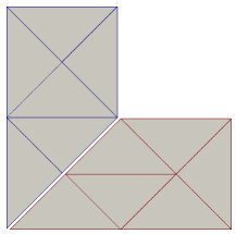
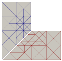
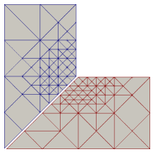
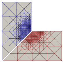
The second example investigates again the accuracy of the three numerical methods but this time we use the L-shaped domain and the transmission problem has the interface defined as the segment going from the reentrant corner to the bottom-left corner of the domain , and the porous domain is the one above the interface. In addition to the singularity of the geometry, we use manufactured solutions with sharp gradients near the reentrant corner
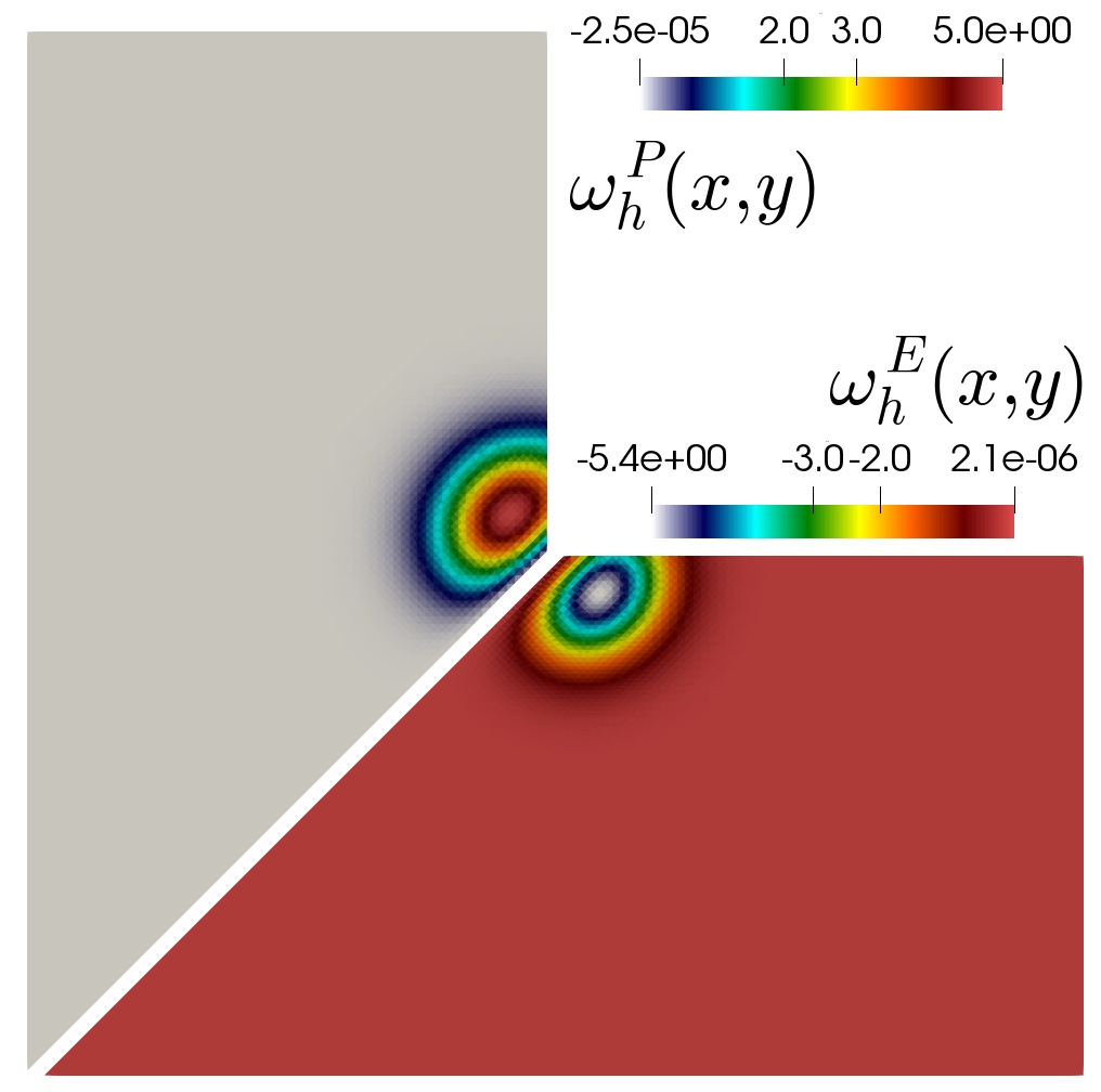
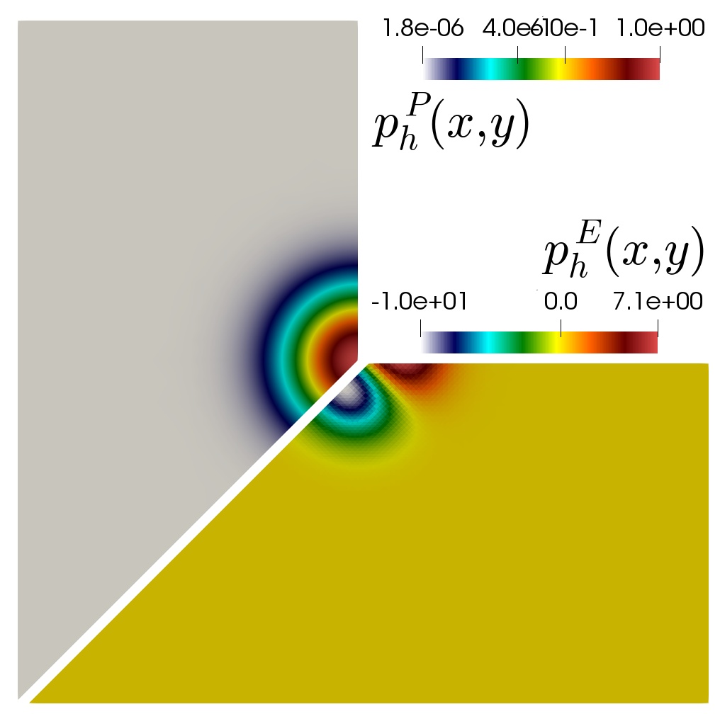
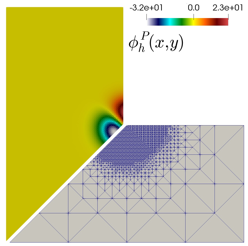
It is expected that the convergence of the methods is hindered due to the lack of regularity of the exact solutions whenever one follows a uniform mesh refinement. Such a slower error decay is clearly observed in the top half of Table 5.4, while adaptive mesh refinement (with a Dörfler constant of ) yields asymptotic optimal convergence evidenced on the bottom half of the table, where also one reaches much smaller errors using a fraction of the degrees of freedom needed in the uniform case. Here we focus on the methods with , and samples of adaptively refine meshes and approximate solutions are portrayed in Figure 5.1. In this case we have used the following contrast of parameters between the subdomains , , , , , , , .
| DoFs | e | |||||||||||||
|---|---|---|---|---|---|---|---|---|---|---|---|---|---|---|
| With uniform mesh refinement | ||||||||||||||
| 157 | 8.56e-01 | – | 7.86e+0 | – | 1.36e+0 | – | 1.61e+0 | – | 9.86e-01 | – | 2.35e+0 | – | 8.246 | 0.071 |
| 575 | 3.80e-01 | 1.17 | 3.05e+0 | 1.37 | 3.64e-01 | 1.90 | 7.07e-01 | 1.19 | 4.15e-01 | 1.25 | 1.16e+0 | 1.02 | 4.199 | 0.151 |
| 2203 | 2.22e-01 | 0.77 | 1.74e+0 | 0.81 | 1.77e-01 | 1.05 | 3.92e-01 | 0.85 | 2.22e-01 | 0.90 | 6.19e-01 | 0.91 | 1.823 | 0.087 |
| 8627 | 7.72e-02 | 1.52 | 4.39e-01 | 1.99 | 4.10e-02 | 2.11 | 1.14e-01 | 1.78 | 5.98e-02 | 1.89 | 1.54e-01 | 2.01 | 0.765 | 0.091 |
| 34147 | 2.66e-02 | 1.54 | 1.09e-01 | 2.01 | 1.09e-02 | 1.92 | 3.45e-02 | 1.72 | 1.58e-02 | 1.92 | 4.10e-02 | 1.91 | 0.319 | 0.034 |
| 135875 | 1.97e-02 | 0.44 | 3.79e-02 | 1.53 | 3.64e-03 | 1.58 | 2.16e-02 | 0.68 | 7.28e-03 | 1.12 | 1.37e-02 | 1.58 | 0.248 | 0.152 |
| With adaptive mesh refinement | ||||||||||||||
| 157 | 8.57e-01 | – | 7.86e+0 | – | 1.36e+0 | – | 1.62e+0 | – | 9.87e-01 | 0.00 | 2.36e+0 | – | 8.239 | 0.081 |
| 551 | 3.79e-01 | 1.30 | 3.05e+0 | 1.51 | 3.65e-01 | 2.10 | 7.07e-01 | 1.32 | 4.17e-01 | 1.37 | 1.16e+0 | 1.13 | 3.201 | 0.081 |
| 1020 | 2.21e-01 | 1.75 | 1.74e+0 | 1.82 | 1.77e-01 | 2.36 | 3.91e-01 | 1.92 | 2.22e-01 | 2.04 | 6.18e-01 | 2.05 | 1.822 | 0.087 |
| 2307 | 7.36e-02 | 2.69 | 4.38e-01 | 3.38 | 4.20e-02 | 3.52 | 1.11e-01 | 3.09 | 5.90e-02 | 3.25 | 1.53e-01 | 3.43 | 0.463 | 0.091 |
| 5779 | 1.81e-02 | 3.06 | 1.06e-01 | 3.10 | 1.21e-02 | 2.71 | 2.74e-02 | 3.04 | 1.45e-02 | 3.06 | 3.96e-02 | 2.94 | 0.112 | 0.089 |
| 20209 | 4.59e-03 | 2.19 | 2.67e-02 | 2.20 | 3.21e-03 | 2.12 | 6.94e-03 | 2.19 | 3.63e-03 | 2.21 | 1.02e-02 | 2.18 | 0.028 | 0.089 |
| 70299 | 1.15e-03 | 2.22 | 6.69e-03 | 2.22 | 1.23e-03 | 1.54 | 1.74e-03 | 2.22 | 9.07e-04 | 2.22 | 2.56e-03 | 2.21 | 0.007 | 0.090 |
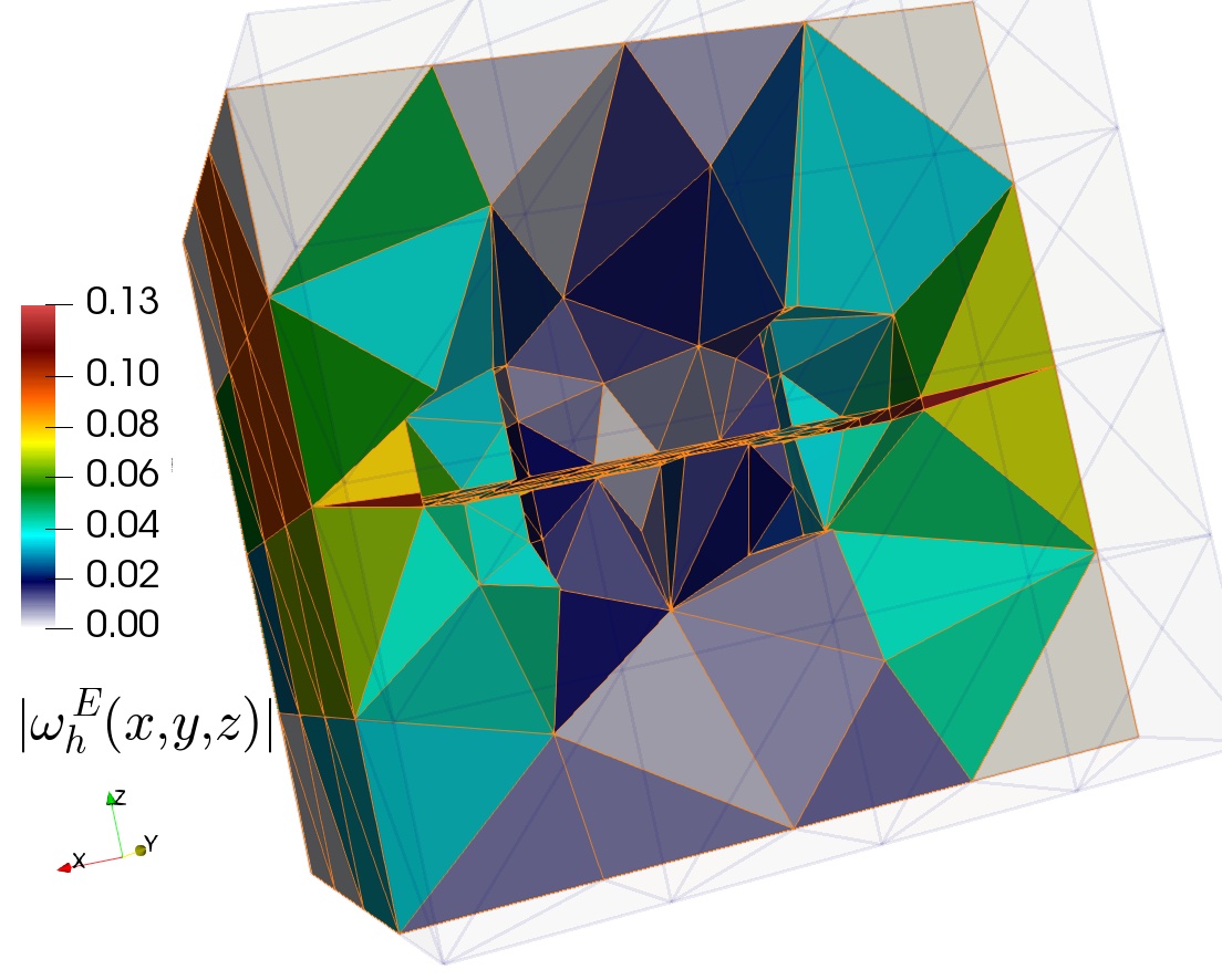
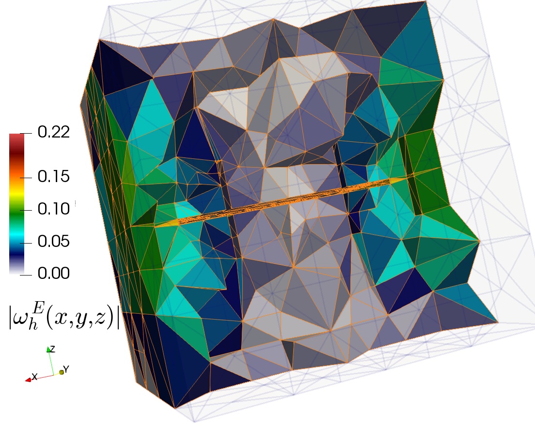
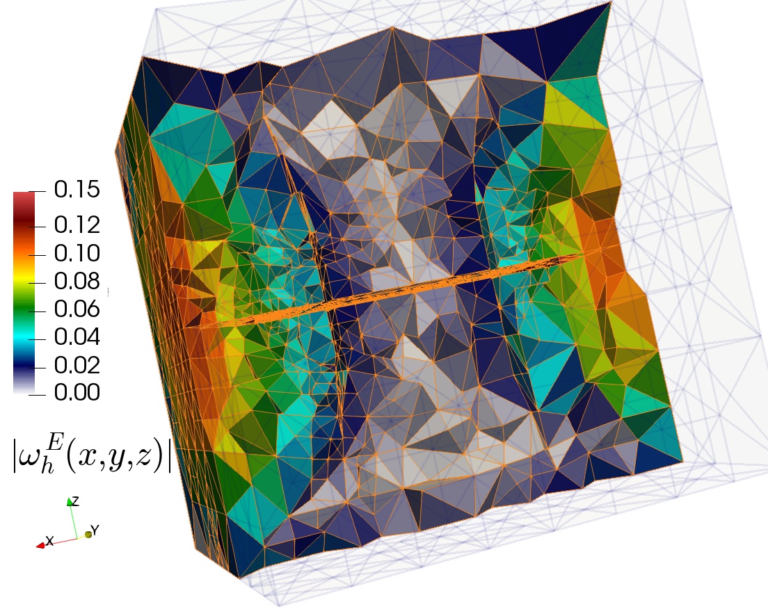
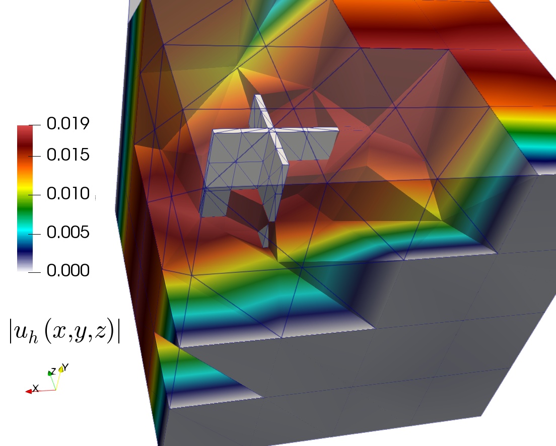
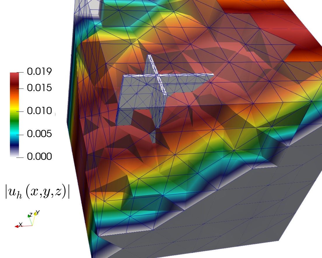
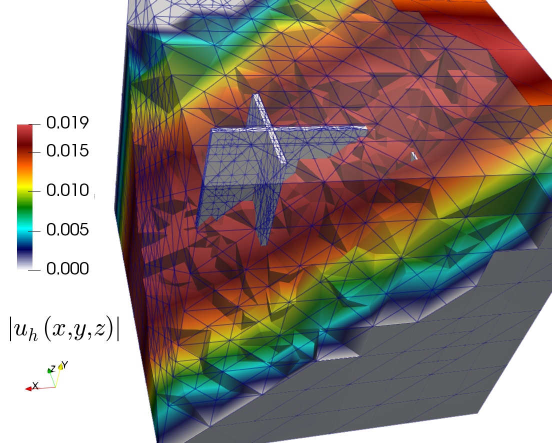
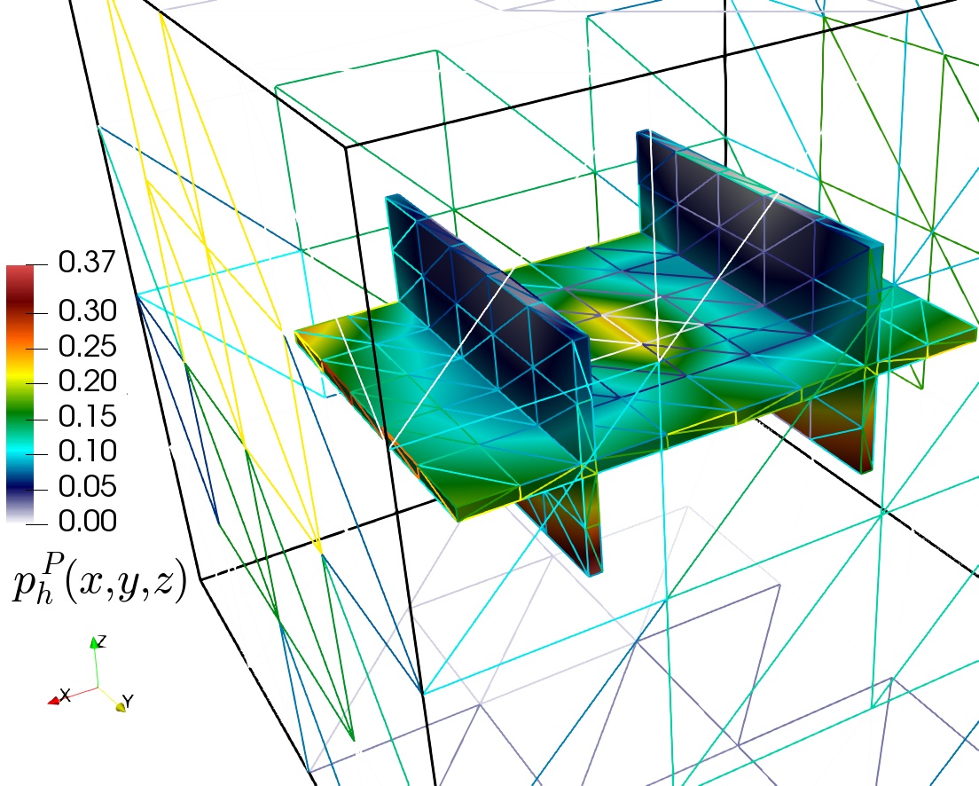
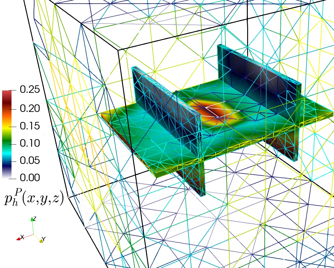
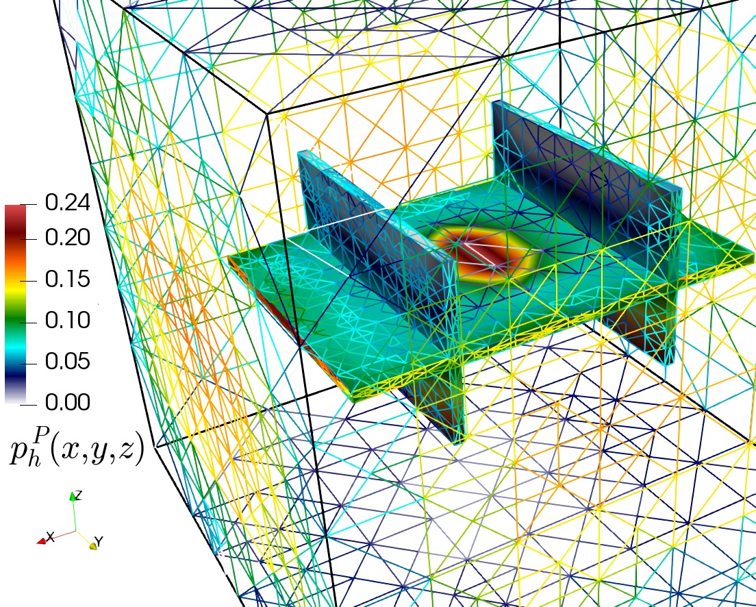
The last test illustrates the use of mesh adaptivity guided by the a posteriori error estimator on an interface elasticity/poroelasticity problem applied to oil reservoir poromechanics, similarly to the test in [15, Sect. 8.2] (see also [17, 3]). In CO2 sequestration in deep subsurface reservoirs one is interested in the distribution of pressure and displacement across the interface between the non-pay rock and the aquifer zones in the case where the poroelastic domain is an array of thin-walled structures fully surrounded by an elastic region. The multi-domain is the unit cube m3 and the aquifer array has a width of 0.015 m. A well is represented by a localised source . This is an injection zone of relatively small radius reaching the centre of the pay zone at . On the surface of the non-pay rock we impose the sliding condition . The interfacial conditions are as in (4.1i). The simulation uses the following values for the model parameters , , , , , , , , , .
Initial coarse meshes are constructed for both subdomains, then we solve the coupled transmission problem, and then apply six steps of the iterative mesh refinement strategy based on the estimator . To observe how the adaptivity takes place on both elastic and poroelastic domains, we plot in Figure 5.2, samples of the approximate solutions on the first three steps of adaptive mesh refinement. The concentration of amount of fluid near the centre of the pay zone is seen in the first row, and we can also see the concentration of refinement near the interface in all panels.
References
- [1] E. Ahmed, F. A. Radu, and J. M. Nordbotten, Adaptive poromechanics computations based on a posteriori error estimates for fully mixed formulations of Biot’s consolidation model, Computer Methods in Applied Mechanics and Engineering, 347 (2019), pp. 264–294.
- [2] M. S. Alnæs, J. Blechta, J. Hake, A. Johansson, B. Kehlet, A. Logg, C. Richardson, J. Ring, M. E. Rognes, and G. N. Wells, The FEniCS project version 1.5, Archive of Numerical Software, 3 (2015), pp. 9–23.
- [3] V. Anaya, Z. De Wijn, B. Gómez-Vargas, D. Mora, and R. Ruiz-Baier, Rotation-based mixed formulations for an elasticity-poroelasticity interface problem, SIAM Journal on Scientific Computing, 42 (2020), pp. B225–B249.
- [4] V. Anaya, Z. De Wijn, D. Mora, and R. Ruiz-Baier, Mixed displacement-rotation-pressure formulations for linear elasticity, Computer Methods in Applied Mechanics and Engineering, 344 (2019), pp. 71–94.
- [5] V. Anaya, B. Gómez-Vargas, D. Mora, and R. Ruiz-Baier, Incorporating variable viscosity in vorticity-based formulations for Brinkman equations, Comptes Rendus Mathématiques, 357 (2019), pp. 552–560.
- [6] S. Atluri and A. Cazzani, Rotations in computational solid mechanics, Archives of Computational Methods in Engineering, 2 (1995), pp. 49–138.
- [7] F. Ballarin, multiphenics – easy prototyping of multiphysics problems in FEniCS. https://mathlab.sissa.it/multiphenics. Accessed: 2021-01-10.
- [8] C. Bernardi and N. Chorfi, Spectral discretization of the vorticity, velocity, and pressure formulation of the Stokes problem, SIAM Journal on Numerical Analysis, 44 (2006), pp. 826–850.
- [9] F. Bertrand and G. Starke, A posteriori error estimates by weakly symmetric stress reconstruction for the Biot problem, Computers and Mathematics with Applications, in press (2021), pp. 1–14.
- [10] F. Brezzi and M. Fortin, Mixed and Hybrid Finite Element Methods, Springer-Verlag, Berlin, 1991.
- [11] W. Dörfler, A convergent adaptive algorithm for Poisson’s equation, SIAM Journal on Numerical Analysis, 33 (1996), pp. 1106–1124.
- [12] F. Dubois, M. Salaün, and S. Salmon, First vorticity–velocity–pressure numerical scheme for the Stokes problem, Computer Methods in Applied Mechanics and Engineering, 192 (2003), pp. 4877–4907.
- [13] A. Ern, Vorticity-velocity formulation of the Stokes problem with variable density and viscosity, Comptes Rendus de l’Académie des Sciences. Série I, 323 (1996), pp. 1159–1164.
- [14] G. N. Gatica, A Simple Introduction to the Mixed Finite Element Method. Theory and Applications, Springer-Verlag, Berlin, 2014.
- [15] V. Girault, X. Lu, and M. F. Wheeler, A posteriori error estimates for Biot system using Enriched Galerkin for flow, Computer Methods in Applied Mechanics and Engineering, 369 (2020), p. e113185.
- [16] V. Girault and P.-A. Raviart, Finite Element Methods for Navier-Stokes Equations: Theory and Algorithms, Springer Publishing Company, 1st ed., 1986.
- [17] V. Girault, M. F. Wheeler, T. Almani, and S. Dana, A priori error estimates for a discretized poro-elastic-elastic system solved by a fixed-stress algorithm, Oil and Gas Science Technology, 74 (2019), p. 24.
- [18] R. Glowinski and O. Pironneau, Numerical methods for the first biharmonic equation and for the two- dimensional Stokes problem, SIAM Review, 21 (1979), pp. 167–212.
- [19] T. Hughes and L. Franca, A new finite element formulation for CFD: VII. The Stokes problem with various well-posed boundary conditions: Symmetric formulations that converge for all velocity/pressure spaces, Comp. Meth. App. Mech. Eng, 65 (1987), pp. 85–96.
- [20] A. Ibrahimbegovic, Finite elastic deformations and finite rotations of 3d continuum with independent rotation field, Revue Européenne des Éléments Finis, 4 (1995), pp. 555–576.
- [21] A. Khan and D. J. Silvester, Robust a posteriori error estimation for mixed finite element approximation of linear poroelasticity, IMA Journal of Numerical Analysis, in press (2020).
- [22] K. Kumar, S. Kyas, J. M. Nordbotten, and S. Repin, Guaranteed and computable error bounds for approximations constructed by an iterative decoupling of the Biot problem, Computers and Mathematics with Applications, in press (2021), pp. 1–14.
- [23] J. Lee, K. Mardal, and R. Winther, Parameter-robust discretization and preconditioning of Biot’s consolidation model, SIAM Journal on Scientific Computing, 39 (2017), pp. A1–A24.
- [24] Y. Li and L. T. Zikatanov, Residual-based a posteriori error estimates of mixed methods for a three-field Biot’s consolidation model, IMA Journal of Numerical Analysis, in press (2020).
- [25] T. Merlini and M. Morandini, The helicoidal modeling in computational finite elasticity. part iii: Finite element approximation for non-polar media, International Journal of Solids and Structures, 42 (2005), pp. 6475–6513.
- [26] J. Nordbotten, T. Rahman, S. Repin, and J. Valdman, A posteriori error estimates for approximate solutions of the Barenblatt-Biot poroelastic model, Computational Methods in Applied Mathematics, 10 (2010), pp. 302–314.
- [27] R. Oyarzúa and R. Ruiz-Baier, Locking-free finite element methods for poroelasticity, SIAM Journal on Numerical Analysis, 54 (2016), pp. 2951–2973.
- [28] R. Verfürth, A posteriori error estimation techniques for finite element methods, OUP Oxford, 2013.
Appendix A Well-posedness analysis for rotation-based poroelasticity
The bilinear forms and the linear functionals appearing in the variational problem (cf. Section 3) of interest are all bounded by constants independent of and [3, 4]. In addition, we have the following result.
Lemma A.1.
Proof.
A.1 Solvability of the continuous problem
Let us rewrite (3.3a)-(3.3c) as: find such that , where the linear operators , , and are defined as
for all , where is the duality pairing between and its dual .
Lemma A.2.
The operator is invertible.
Proof.
First, for a given functional , observe that establishing the invertibility of is equivalent to proving the unique solvability of the operator problem
| (A.2) |
Furthermore, proving unique solvability of (A.2) is in turn equivalent to proving the unique solvability of the two following uncoupled problems: find such that
| (A.3) | ||||
and: find , such that
| (A.4) |
where , , and are the functionals induced by , , and , respectively. The unique solvability of (A.4) follows by virtue of the Lax-Milgram lemma, and the well-posedness of (A.3) follows from a straightforward application of the Babuška-Brezzi theory.
Lemma A.3.
The operator is compact.
Proof.
We begin by defining the operator as
This operator is the composition of a compact injection and a continuous map and it is therefore compact. And denoting by the adjoint of , we infer that the following map is also compact
Lemma A.4.
The operator is injective.
Proof.
It is sufficient to show that the only solution to the homogeneous problem
is the null-vector in . Thus, from Lemma A.1, and the fact that , we have , , .
Appendix B A priori error analysis for rotation-based poroelasticity
B.1 Stability of the discrete problem
All bilinear forms and functionals introduced in Section 3 preserve stability on the discrete spaces. Also, , and maintain coercivity on and , respectively. Such stability properties permit us to establish the well-posedness of (B.1)-(B.3).
Theorem B.1.
B.2 A priori error bounds
Approximation properties of the spaces in (3.4) (see, e.g., [10]) produce the following theoretical rate of convergence:
where , , and .
Theorem B.2.
Proof.
Using triangle inequality we can split the error into two parts
Then we can estimate the first term thanks to approximation results. To estimate the second term, we use the stability result given in Theorem 3.1, then
with . We can then invoke the continuity results to get