Revisiting the Weaknesses of Reinforcement Learning
for Neural Machine Translation

Abstract

Policy gradient algorithms have found wide adoption in NLP, but have recently become subject to criticism, doubting their suitability for NMT. Choshen et al. (2020) identify multiple weaknesses and suspect that their success is determined by the shape of output distributions rather than the reward. In this paper, we revisit these claims and study them under a wider range of configurations. Our experiments on in-domain and cross-domain adaptation reveal the importance of exploration and reward scaling, and provide empirical counter-evidence to these claims.

1 Introduction

In neural sequence-to-sequence learning, in particular Neural Machine Translation (NMT), Reinforcement Learning (RL) has gained attraction due to the suitability of Policy Gradient (PG) methods for the end-to-end training paradigm (Ranzato et al., 2016; Li et al., 2016; Yu et al., 2017; Li et al., 2018; Flachs et al., 2019; Sankar and Ravi, 2019). The idea is to let the model explore the output space beyond the reference output that is used for standard cross-entropy minimization, by reinforcing model outputs according to their quality, effectively increasing the likelihood of higher-quality samples. The classic exploration-exploitation dilemma from RL is addressed by sampling from a pretrained model’s softmax distribution over output tokens, such that the model entropy steers exploration.

For the application of NMT, it was firstly utilized to bridge the mismatch between the optimization for token-level likelihoods during training and the corpus-level held-out set evaluations with non-differentiable/decomposable metrics like BLEU (Ranzato et al., 2016; Edunov et al., 2018), and secondly to reduce exposure bias in autoregressive sequence generators (Ranzato et al., 2016; Wang and Sennrich, 2020). It has furthermore been identified as a promising tool to adapt pretrained models to new domains or user preferences by replacing reward functions with human feedback in human-in-the-loop learning (Sokolov et al., 2016; Nguyen et al., 2017).

Recently, the effectiveness of these methods has been questioned: Choshen et al. (2020) identify multiple theoretical and empirical weaknesses, leading to the suspicion that performance gains with RL in NMT are not due to the reward signal. The most surprising result is that the replacement of a meaningful reward function (giving higher rewards to higher-quality translations) by a constant reward (reinforcing all model samples equally) yields similar improvements in BLEU. To explain this counter-intuitive result, Choshen et al. (2020) conclude that a phenomenon called the peakiness effect must be responsible for performance gains instead of the reward. This means that the most likely tokens in the beginning gain probability mass regardless of the rewards they receive during RL training. If this hypothesis was true, then the perspectives for using methods of RL for encoding real-world preferences into the model would be quite dire, as models would essentially be stuck with whatever they learned during supervised pretraining and not reflect the feedback they obtain later on.

However, the analysis by Choshen et al. (2020) missed a few crucial aspects of RL that have led to empirical success in previous works: First, variance reduction techniques such as the average reward baseline were already proposed with the original Policy Gradient by Williams (1992), and proved effective for NMT (Kreutzer et al., 2017; Nguyen et al., 2017). Second, the exploration-exploitation trade-off can be controlled by modifying the sampling function (Sharaf and Daumé III, 2017), which in turn influences the peakiness.

We therefore revisit the previous findings with NMT experiments differentiating model behavior between in-domain and out-of-domain adaptation, controlling exploration, reducing variance, and isolating the effect of reward scaling. This allows us to establish a more holistic view of the previously identified weaknesses of RL. In fact, our experiments reveal that improvements in BLEU can not solely be explained by increased peakiness, and that simple methods encouraging stronger exploration can successfully move previously lower-ranked token into higher ranks. We observe generally low empirical gains in in-domain adaptation, which might explain the surprising success of constant rewards in Choshen et al. (2020). However, we find that rewards and their scaling do matter for domain adaptation. Furthermore, our results corroborate the auspicious findings of  Wang and Sennrich (2020) that RL mitigates exposure bias. Our paper thus reinstates the potential of RL for model adaptation in NMT, and puts previous pessimistic findings into perspective. The code for our experiments is publicly available.

2 RL for NMT

The objective of RL in NMT is to maximize the expected reward for the model’s outputs with respect to the parameters $\theta$: $\arg\max_{\theta}\mathbb{E}_{p_{\theta}(y\mid x)}[\Delta(y,y^{\prime})]$. where $y^{\prime}$ denotes a reference translation, $y$ is the generated translation and $\Delta$ is a metric (e.g. BLEU (Papineni et al., 2002)), rewarding similarities to the reference. Applying the log derivative trick, the following gradient can be derived:

$$\nabla_{\theta}=\mathbb{E}_{p_{\theta}(y\mid x)}[\Delta(y,y^{\prime})\nabla_{\theta}\log p_{\theta}(y\mid x)].$$ (1)

The benefit of Eq. 1 is that it does not require differentiation of $\Delta$ which allows for direct optimization of the BLEU score or human feedback.

2.1 Policy Gradient

However, computing the gradient requires the summation over all $y\in\mathcal{V}_{trg}^{m}$, which is computationally infeasible for large sequence lengths $m$ and vocabulary sizes $\mathcal{V}_{trg}$ as they are common in NMT. Therefore, Eq. 1 is usually approximated through Monte Carlo sampling (Williams, 1992) resulting in unbiased estimators of the full gradient.

We draw one sample from the multinomial distribution defined by the model’s softmax to approximate Eq. 1 (Ranzato et al., 2016; Kreutzer et al., 2017; Choshen et al., 2020), which results in the following update rule with learning rate $\alpha$:

$$u_{k}=\nabla_{\theta}\log p_{\theta}(y\mid x)\Delta(y,y^{\prime})$$ (2)

$$\theta_{t+1}=\theta_{t}+\alpha u_{k}$$ (3)

2.2 Softmax Temperature

The temperature $\tau$ of the softmax distribution $\exp(y_{i}/\tau)/\sum_{j}\exp(y_{j}/\tau)$ can be used to control the amount of exploration during learning. Setting $0<\tau<1$ results in less diverse samples while setting $\tau>1$ increases the diversity and also the entropy of the distribution. Lowering the temperature (i.e. making the distribution peakier) may be used to make policies more deterministic towards the end of training (Sutton and Barto, 1998; Rose, 1998; Sokolov et al., 2017), while we aim to reduce peakiness by increasing the temperature.

Model	$\Delta p_{top10}$	$\Delta p_{mode}$	BLEU ($k=1$)	BLEU ($k=5$)	BLEU ($k=50$)
Pretraining (IWSLT14)	0	0	33.49	34.12	33.88
PG ($n=1$)	11.46	24.82	$33.84\pm 0.05$	$34.24\pm 0.04$	$34.16\pm 0.13$
PG + scaled	11.36	24.42	$33.91\pm 0.14$	$34.30\pm 0.10$	$34.19\pm 0.11$
PG + average bl	12.54	27.84	$34.20\pm 0.04$	$34.40\pm 0.03$	$34.30\pm 0.04$
PG + $\tau=1.2$	6.08	16.91	$33.88\pm 0.04$	$34.15\pm 0.02$	$34.11\pm 0.01$
PG + $\tau=0.8$	14.29	29.74	$33.80\pm 0.03$	$34.26\pm 0.11$	$34.14\pm 0.10$
PG + constant	1.42	1.02	$33.53\pm 0.04$	$34.13\pm 0.01$	$33.91\pm 0.03$
PG + average bl + $\tau=1.05$	12.09	27.51	$34.37\pm 0.06$	$34.51\pm 0.11$	$34.46\pm 0.09$
PG + average bl + $\tau=0.95$	13.36	29.83	$34.28\pm 0.10$	$34.51\pm 0.06$	$34.41\pm 0.09$
MRT ($n=5$)	12.93	32.85	$34.52\pm 0.06$	$34.68\pm 0.05$	$34.63\pm 0.05$

Table 1: In-domain adaptation: Peakiness indicators (%), and IWSLT14 test set results for beam size $k$.

2.3 Modified Rewards

Variance reduction techniques were already suggested by Williams (1992) and found to improve generalization for NMT (Kreutzer et al., 2017). The simplest option is the baseline reward, which in practice is realized by subtracting a running average of historic rewards from the current reward $\Delta$ in Eq. 2. It represents an expected reward, so that model outputs get more strongly reinforced or penalized if they diverge from it.

In addition to variance reduction, subtracting baseline rewards also change the scale of rewards (e.g. $\Delta\in[0,1]$ for BLEU becomes $\Delta\in[-0.5,0.5]$), allowing updates towards or away from samples by switching the sign of $u_{k}$ (Eq. 2). The same range of rewards can be obtained by re-scaling them, e.g., to $\frac{\Delta(y,y^{\prime})-\min}{\max-\min}-0.5$ with the minimum ($\min$) and maximum ($\max$) $\Delta$ within each batch.

2.4 Minimum Risk Training

Minimum Risk Training (MRT) (Shen et al., 2016) aims to minimize the empirical risk of task loss over a larger set of $n=|\mathcal{S}|,n>1$ output samples $\mathcal{S}(x)\subset{Y}(x)$:

$$\arg\min_{\theta}\sum_{(x,y^{\prime})\in\mathcal{D}}\sum_{y\in\mathcal{S}(x)}{Q}_{\theta,\alpha}(y\mid x)[-\Delta(y,y^{\prime})],$$

$${Q}_{\theta,\alpha}(y\mid x^{(s)})=\frac{p_{\theta}(y\mid x)^{\alpha}}{\sum_{y^{\prime\prime}\in\mathcal{S}(x)}p_{\theta}(y^{\prime\prime}\mid x)^{\alpha}}.$$

As pointed out by Choshen et al. (2020), MRT learns with biased stochastic estimates of the RL objective due to the renormalization of model scores, but that has not hindered its empirical success (Shen et al., 2016; Edunov et al., 2018; Wieting et al., 2019; Wang and Sennrich, 2020). Interestingly, the resulting gradient update includes a renormalization of sampled rewards, yielding a similar effect to the baseline reward (Shen et al., 2016). It also allows for more exploration thanks to learning from multiple samples per input, but it is therefore less attractive for human-in-the-loop learning and efficient training.

2.5 Exposure Bias

The exposure bias in NMT arises from the model only being exposed to the ground truth during training, and receiving its own previous predictions during inference—while it might be overly reliant on perfect context, which in turn lets errors accumulate rapidly over long sequences (Ranzato et al., 2016). Wang and Sennrich (2020) hypothesize that exposure bias increases the prevalence of hallucinations in domain adaptation and causes the beam search curse (Koehn and Knowles, 2017; Yang et al., 2018), which describes the problem that the model’s performance worsens with large beams. Wang and Sennrich (2020) find that MRT with multiple samples can mitigate this problem thanks to being exposed to model predictions during training. We will extend this finding to other PG variants with single samples.

3 Experiments

We implement PG and MRT (without enforcing gold tokens in $\mathcal{S}$; $n=5$) in Joey NMT (Kreutzer et al., 2019) for Transformers (Vaswani et al., 2017). We simulate rewards for training samples from IWSLT14 de-en with sacreBLEU (Post, 2018), and test on IWSLT14 held-out sets. We consider two different domains for pretraining, WMT15 and IWSLT14. This allows us to distinguish the effects of RL in in-domain learning vs domain adaptation scenarios. RL experiments are repeated three times and we report mean and standard deviation. Remaining experimental details can be found in the Appendix. The goal is not to find the best model in a supervised domain adaptation setup (“Fine-tuning” in Table 2), but to investigate if/how scalar rewards expressing translation preferences can guide learning, mimicking a human-in-the-loop learning scenario.

3.1 Peakiness

Choshen et al. (2020) suspect that PG improvements are due to an increase in peakiness. Increased peakiness is indicated by a disproportionate rise of $p_{top10}$ and $p_{mode}$, the average token probability of the 10 most likely tokens, and the mode, respectively. To test the influence of peakiness on performance, we deliberately increase and decrease the peakiness of the output distribution by adjusting the parameter $\tau$. In Tables 1 and  2 we can see that all PG variants generally increase peakiness ($p_{top10}$ and $p_{mode}$), but that those with higher temperature $\tau>1$ show a lower increase. Comparing the peakiness with the BLEU scores, we find that BLEU gains are not tied to increasing peakiness in in-domain and cross-domain adaptation experiments. This is exemplified by reward scaling (“PG+scaled”), which improves the BLEU but does not lead to an increase in peakiness compared to PG. These results show that improvements in BLEU can not just be explained by the peakiness effect. However, in cross-domain adaptation exploration plays a major role: Since the model is less familiar with the new data, reducing exploration (lower $\tau$) helps to improve translation quality.

3.2 Upwards Mobility

One disadvantage of high peakiness is that previously likely tokens accumulate even more probability mass during RL. Choshen et al. (2020) therefore fear that it might be close to impossible to transport lower-ranking tokens to higher ranks with RL. We test this hypothesis under different exploration settings by counting the number of gold tokens in each rank of the output distribution. That number is divided by the number of all gold tokens to obtain the probability of gold tokens appearing in each rank. We then compare the probability before and after RL. Fig. 1 illustrates that training with an increased temperature pushes more gold tokens out of the lowest rank. The baseline reward has a beneficial effect to that aim, since it allows down-weighing samples as well. This shows that upwards mobility is feasible and not a principled problem for PG.

Model	$\Delta p_{top10}$	$\Delta p_{mode}$	BLEU ($k=1$)	BLEU ($k=5$)	BLEU ($k=50$)
Pretraining (WMT15)	0	0	19.74	20.35	20.10
Self-training (IWSLT14)	46.87	99.15	$19.74\pm 0.00$	$20.35\pm 0.00$	$20.10\pm 0.00$
Fine-Tuning (IWSLT14)	16.71	25.29	$28.25\pm 0.11$	$29.38\pm 0.09$	$29.48\pm 0.05$
PG ($n=1$)	44.10	88.60	$22.34\pm 0.73$	$22.62\pm 0.56$	$22.60\pm 0.51$
PG + scaled	43.46	87.83	$23.23\pm 0.12$	$23.50\pm 0.15$	$23.52\pm 0.19$
PG + average bl	44.91	94.65	$24.31\pm 0.41$	$24.53\pm 0.26$	$24.56\pm 0.22$
PG + $\tau=1.2$	39.05	78.93	$21.26\pm 0.20$	$21.58\pm 0.21$	$21.60\pm 0.28$
PG + $\tau=0.8$	46.91	95.10	$23.27\pm 0.24$	$23.82\pm 0.22$	$23.93\pm 0.23$
PG + constant	48.50	115.31	$19.74\pm 0.00$	$20.35\pm 0.00$	$20.10\pm 0.00$
PG + average bl + $\tau=1.05$	44.44	93.53	$24.18\pm 0.09$	$24.53\pm 0.09$	$24.60\pm 0.11$
PG + average bl + $\tau=0.95$	45.34	95.04	$24.41\pm 0.30$	$24.86\pm 0.17$	$24.86\pm 0.11$
MRT ($n=5$)	44.63	103.68	$26.98\pm 0.10$	$27.08\pm 0.09$	$27.09\pm 0.10$

Table 2: Cross-domain adaptation: Peakiness indicators (%), and IWSLT14 test set results for beam size $k$.

3.3 Meaningful Rewards

Choshen et al. (2020) observe an increase in peakiness when all rewards are set to 1, and BLEU improvements even comparable to BLEU rewards. While our results with a constant reward of 1 (“PG+constant”) also show an increase in peakiness for cross-domain adaptation (Table 2), we observe deteriorating scores using the same hyperparameters as with other PG variants. Reducing the learning rate from $1\times 10^{-4}$ to $1\times 10^{-5}$ alleviates these effects but still does not lead to notable improvements over the pretrained model (with an average gain of 0.09 BLEU). Similarly, domain adaptation via self-training increases peakiness but does not show improvements over the baseline. A smaller learning rate of $1\times 10^{-5}$ reduces peakiness and shows a similar behaviour as constant rewards (a gain of 0.1 BLEU). These results confirm that gains do not come from being exposed to new inputs and increased peakiness, which contradicts the results of Choshen et al. (2020). While the effects in-domain are generally weak with a maximum gain of 0.5 BLEU over the baseline (with beam size $k=5$, Table 1), the results for domain adaptation (Table 2) show a clear advantage of using informative rewards with up to +4.5 BLEU for PG and +6.7 BLEU for MRT (with beam size $k=5$). We conclude that rewards do matter for PG for NMT.

3.4 Allowing Negative Rewards

As described in Section 2.3, scaling the reward (“PG+scaled”), subtracting a baseline (“PG+average bl”), or normalizing it over multiple samples for MRT, introduces negative rewards, which enables updates away from sampled outputs. BLEU under domain shift (Table 2) shows a significant improvement when allowing negative rewards. The scaled reward increases the score by almost 1 BLEU, the average reward baseline by almost 2 BLEU and MRT leads to a gain of about 4.5 BLEU over plain PG.

3.5 The Beam Curse

The results show that improvements of RL over the baseline are higher with lower beam sizes, since RL reduces the need for exploration (through search) during inference thanks to the exploration during training. These findings are in line with Bahdanau et al. (2017). For RL models, BLEU reductions caused by larger beams are weaker than for the baseline model in both settings, which confirms that PG methods are effective at mitigating the beam search problem, and according to Wang and Sennrich (2020) might also reduce hallucinations.

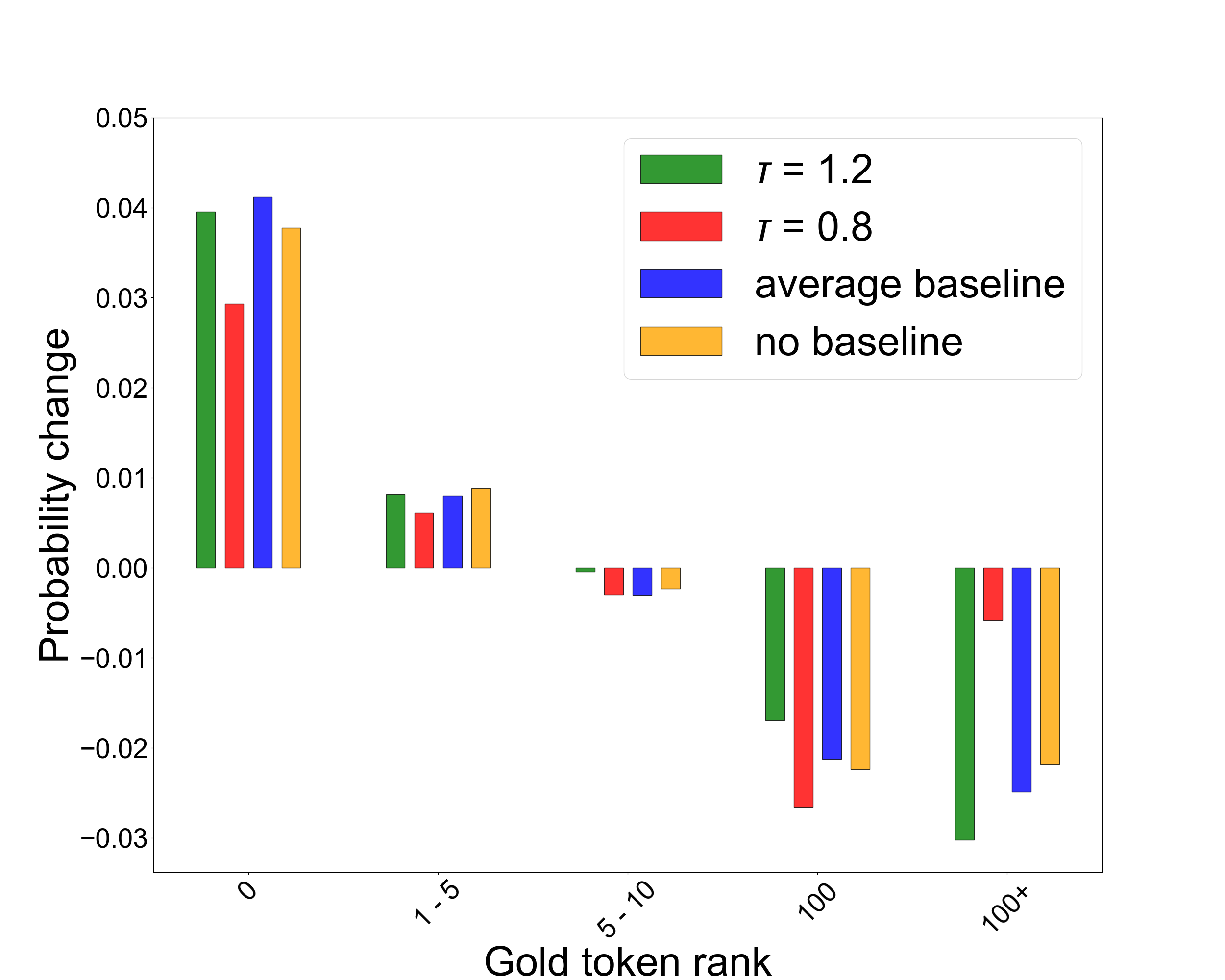
Figure 1: Change in probability for gold tokens to belong to each rank before and after RL on in-domain data.

3.6 Discussion

Despite the promising empirical gains over a pretrained baseline, all above methods would fail if trained from scratch, as there are no non-zero-reward translation outputs sampled when starting from a random policy. Empirical improvements over a strong pretrained model vanish when there is little to learn from the new feedback, e.g. when it is given on the same data which the model was already trained on, as we have shown above, relating to the “failure” cases in Choshen et al. (2020). RL methods for MT can be effective at adapting a model to new custom preferences if these preferences can be reflected in an appropriate reward function, which we simulated with in-domain data. In Table 2, we observed this effect and gained several BLEU points without revealing reference translations to the model. Being exposed to new sources alone (without rewards) is not sufficient to obtain improvements, which we tested by self-training (Table 2). Ultimately, the potential to improve MT models with RL methods lies in situations where there are no reference translations but reward signals, and models can be pretrained on existing data.

4 Conclusion

We provided empirical counter-evidence for some of the claimed weaknesses of RL in NMT by untying BLEU gains from peakiness, showcasing the upwards mobility of low-ranking tokens, and re-confirming the importance of reward functions. The affirmed gains of PG variants in adaptation scenarios and their responsiveness to reward functions, combined with exposure bias repair and avoidance of the beam curse, rekindle the potential to utilize them for adapting models to human preferences.

Appendix A Data

Domain	Train	Dev	Test
WMT15	$3\,898\,886$	$8496$	$2902$
IWSLT14	$159\,392$	$7245$	$6750$

Table 3: Training, dev, and test sizes for WMT15 and IWSLT14 de-en data in number of sentences.

Table 3 lists the sizes of data split for the parallel datasets from WMT15 (Bojar et al., 2015) and IWSLT14 used in the experiments. The two datasets are preprocessed using scripts from the Moses toolkit. The preprocessing pipeline contains the following steps:

• Tokenization with tokenizer.perl

• Lowercasing with lowercase.perl

• Filtering using clean-corpus-n.perl. Sentences with more than 80 words are removed from the dataset

Additionally, we applied Byte-Pair-Encoding (Sennrich et al., 2016) using subword-nmt to create subword units.

Appendix B Model Configurations

Table 8 contains the hyperparameters as Joey NMT configurations for the pretrained models, Table 9 the modified hyperparameters for PG, and Table 10 the modified hyperparameters for MRT. Random seeds for the three runs were set to 42, 8 and 64.

Appendix C Sample Efficiency

Fig. 2 shows that both MRT and Policy Gradient need a comparable amount of steps (with a batch size of 256 tokens) to reach their optimum. However, the performance of MRT is more stable over the course of training, while Policy Gradient shows higher variance. MRT learns from $n=5$ outputs and rewards per step (compared to Policy Gradient with $n=1$), which stabilizes the updates.

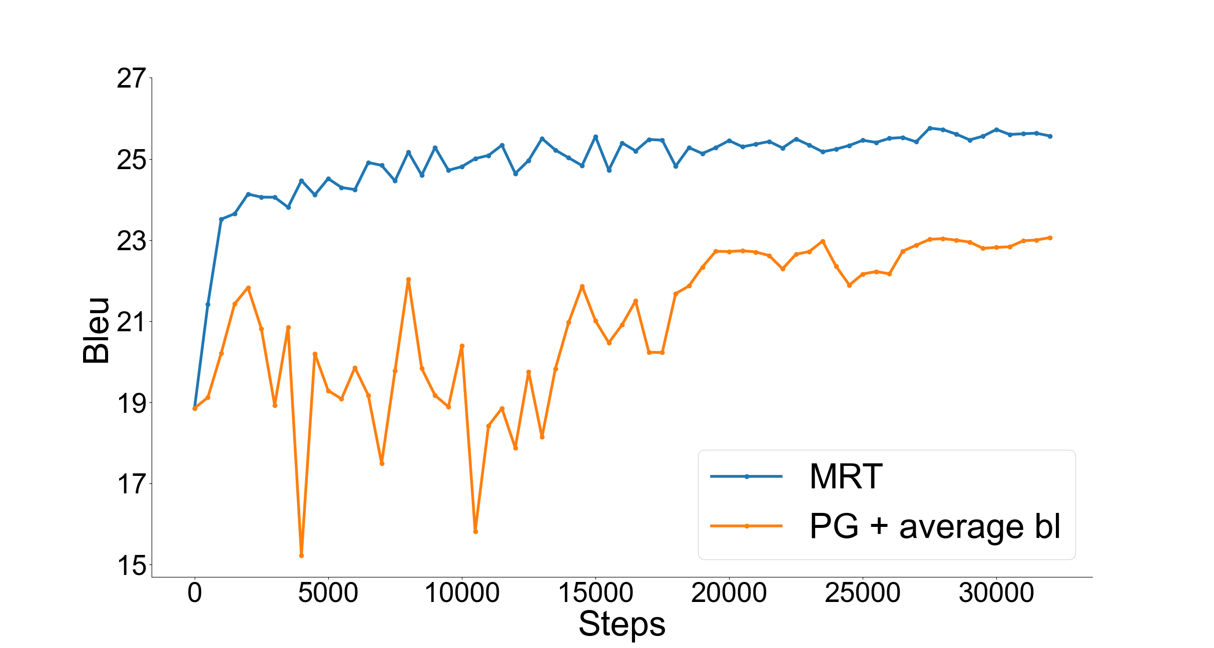
Figure 2: Dev BLEU/steps for cross-domain.

Appendix D Additional Considerations

Learned Baseline

A reward baseline can also be learned by formulating it as a regression problem, but like Wu et al. (2018) we found no empirical gains, thus excluded it from the experiments reported in this paper.

Scaling Rewards

We found that selecting $max$ and $min$ over all previous rewards led to deteriorating BLEU scores. This is why we recompute them for each batch.

Gold Tokens in MRT

Shen et al. (2016) add the gold sequence to the sample space. However, Edunov et al. (2018) find that this destabilizes training, so Choshen et al. (2020) and Wang and Sennrich (2020) choose to omit it, and so do we.

Appendix E Development Results

Tables 4 and 5 report results on the development set that were used for tuning the models. They show stable results across different held-out sets.

Appendix F Absolute Peakiness

Tables 7 and  6 contain the absolute values for the change in peakiness that were used to compute percentages for the main paper results.

Model	Dev BLEU	Test BLEU
Pretraining	34.26	34.12
PG	$34.37\pm 0.12$	$34.24\pm 0.04$
PG + average bl	$34.75\pm 0.06$	$34.40\pm 0.03$
PG + $\tau=1.2$	$34.46\pm 0.10$	$34.15\pm 0.02$
PG + $\tau=0.8$	$34.47\pm 0.12$	$34.26\pm 0.11$
PG + constant	$34.26\pm 0$	$34.13\pm 0.01$
PG + scaled	$34.55\pm 0.10$	$34.30\pm 0.10$

Table 4: PG variants in-domain adaptation (IWSLT14), beam size=5.

Model	Dev BLEU	Test BLEU
Pretraining	18.86	20.35
PG	$21.63\pm 0.39$	$22.62\pm 0.56$
PG + average bl	$23.31\pm 0.32$	$24.53\pm 0.26$
PG + $\tau=1.2$	$20.45\pm 0.18$	$21.58\pm 0.21$
PG + $\tau=0.8$	$22.42\pm 0.08$	$23.82\pm 0.22$
PG + constant	$18.86\pm 0$	$20.35\pm 0$
PG + scaled	$22.40\pm 0.10$	$23.50\pm 0.15$

Table 5: PG variants cross-domain adaptation (WMT15 to IWSLT14), beam size=5

Model	$\Delta p_{top10}$	$\Delta p_{mode}$	$\Delta p_{gold}$
PG	$0.294\pm 0.001$	$0.400\pm 0.001$	$0.095\pm 0.002$
PG + scaled	$0.290\pm 0.002$	$0.397\pm 0.006$	$0.098\pm 0.001$
PG + average bl	$0.300\pm 0.001$	$0.428\pm 0.001$	$0.103\pm 0.002$
PG + $\tau=1.2$	$0.260\pm 0.003$	$0.357\pm 0.006$	$0.082\pm 0.001$
PG + $\tau=0.8$	$0.313\pm 0.001$	$0.430\pm 0.001$	$0.102\pm 0.001$
PG + constant	$0.323\pm 0.001$	$0.521\pm 0.002$	$-0.123\pm 0.004$
MRT	$0.307\pm 0.002$	$0.482\pm 0.004$	$0.126\pm 0.004$

Table 6: Absolute changes in peakiness for cross-domain adaptation (WMT15 to IWSLT14).

Model	$\Delta p_{top10}$	$\Delta p_{mode}$	$\Delta p_{gold}$
PG	$0.099\pm 0.002$	$0.199\pm 0.003$	$0.076\pm 0.001$
PG + scaled	$0.097\pm 0.002$	$0.162\pm 0.005$	$0.074\pm 0.002$
PG + average bl	$0.108\pm 0.002$	$0.185\pm 0.006$	$0.083\pm 0.002$
PG + $\tau=1.2$	$0.052\pm 0.002$	$0.112\pm 0.004$	$0.060\pm 0.001$
PG + $\tau=0.8$	$0.123\pm 0.001$	$0.198\pm 0.003$	$0.083\pm 0.003$
PG + constant	$0.012\pm 0.007$	$0.017\pm 0.007$	$0.003\pm 0.001$
MRT	$0.112\pm 0.003$	$0.217\pm 0.004$	$0.090\pm 0.004$

Table 7: Absolute changes in peakiness for in-domain (IWSLT14) adaptation.

Model	IWSLT14	WMT15
Parameter	Setting	Setting
initializer	"xavier"	"xavier"
embed initializer	"xavier"	"xavier"
embed init gain	1.0	1.0
init gain	1.0	1.0
bias initializer	"zeros"	"zeros"
tied embeddings	True	True
tied softmax	True	True
encoder type	Transformer	Transfomer
encoder embeddings dim	256	128
encoder hidden size	256	128
encoder dropout	0.3	0.3
encoder num layers	6	6
encoder num heads	4	4
encoder ff_size	1024	512
decoder type	Transformer	Transformer
decoder embeddings dim	256	128
decoder hidden size	256	128
decoder dropout	0.3	0.3
decoder num layers	6	6
decoder num heads	4	4
decoder ff_size	1024	512
optimizer	"adam"	"adam"
normalization	"tokens"	"tokens"
adam_betas	[0.9, 0.999]	[0.9, 0.999]
scheduling	"plateau"	"plateau"
patience	5	5
decrease_factor	0.7	0.7
loss	"crossentropy"	"crossentropy"
learning rate	0.0003	0.0003
learning rate_min	0.00000002	0.00000002
weight decay	0.0	0.0
label smoothing	0.1	0.1
batch size	2048	4096
batch type	"token"	"token"
epochs	100	100

Table 8: Pretraining model parameters

Parameter	In-domain	Cross-domain
learning rate	0.00001	0.0001
batch size	128	256

Table 9: Policy Gradient parameters

Parameter	In-domain	Cross-domain
learning rate	0.00001	0.0001
batch size	32	64
batch multiplier	4	4
eval batch size	128	128
samples	5	5
alpha	0.005	0.005

Table 10: MRT parameters

References

- Bahdanau et al. (2017) Dzmitry Bahdanau, Philemon Brakel, Kelvin Xu, Anirudh Goyal, Ryan Lowe, Joelle Pineau, Aaron C. Courville, and Yoshua Bengio. 2017. An actor-critic algorithm for sequence prediction. In 5th International Conference on Learning Representations, ICLR 2017, Toulon, France, April 24-26, 2017, Conference Track Proceedings.
- Bojar et al. (2015) Ondřej Bojar, Rajen Chatterjee, Christian Federmann, Barry Haddow, Matthias Huck, Chris Hokamp, Philipp Koehn, Varvara Logacheva, Christof Monz, Matteo Negri, Matt Post, Carolina Scarton, Lucia Specia, and Marco Turchi. 2015. Findings of the 2015 workshop on statistical machine translation. In Proceedings of the Tenth Workshop on Statistical Machine Translation, pages 1–46, Lisbon, Portugal. Association for Computational Linguistics.
- Choshen et al. (2020) Leshem Choshen, Lior Fox, Zohar Aizenbud, and Omri Abend. 2020. On the weaknesses of reinforcement learning for neural machine translation. In 8th International Conference on Learning Representations, ICLR 2020, Addis Ababa, Ethiopia, April 26-30, 2020.
- Edunov et al. (2018) Sergey Edunov, Myle Ott, Michael Auli, David Grangier, and Marc’Aurelio Ranzato. 2018. Classical structured prediction losses for sequence to sequence learning. In Proceedings of the 2018 Conference of the North American Chapter of the Association for Computational Linguistics: Human Language Technologies, Volume 1 (Long Papers), pages 355–364, New Orleans, Louisiana. Association for Computational Linguistics.
- Flachs et al. (2019) Simon Flachs, Marcel Bollmann, and Anders Søgaard. 2019. Historical text normalization with delayed rewards. In Proceedings of the 57th Annual Meeting of the Association for Computational Linguistics, pages 1614–1619, Florence, Italy. Association for Computational Linguistics.
- Koehn and Knowles (2017) Philipp Koehn and Rebecca Knowles. 2017. Six challenges for neural machine translation. In Proceedings of the First Workshop on Neural Machine Translation, pages 28–39, Vancouver. Association for Computational Linguistics.
- Kreutzer et al. (2019) Julia Kreutzer, Jasmijn Bastings, and Stefan Riezler. 2019. Joey NMT: A minimalist NMT toolkit for novices. In Proceedings of the 2019 Conference on Empirical Methods in Natural Language Processing and the 9th International Joint Conference on Natural Language Processing (EMNLP-IJCNLP): System Demonstrations, pages 109–114, Hong Kong, China. Association for Computational Linguistics.
- Kreutzer et al. (2017) Julia Kreutzer, Artem Sokolov, and Stefan Riezler. 2017. Bandit structured prediction for neural sequence-to-sequence learning. In Proceedings of the 55th Annual Meeting of the Association for Computational Linguistics (Volume 1: Long Papers), pages 1503–1513, Vancouver, Canada. Association for Computational Linguistics.
- Li et al. (2016) Jiwei Li, Will Monroe, Alan Ritter, Dan Jurafsky, Michel Galley, and Jianfeng Gao. 2016. Deep reinforcement learning for dialogue generation. In Proceedings of the 2016 Conference on Empirical Methods in Natural Language Processing, pages 1192–1202, Austin, Texas. Association for Computational Linguistics.
- Li et al. (2018) Zichao Li, Xin Jiang, Lifeng Shang, and Hang Li. 2018. Paraphrase generation with deep reinforcement learning. In Proceedings of the 2018 Conference on Empirical Methods in Natural Language Processing, pages 3865–3878, Brussels, Belgium. Association for Computational Linguistics.
- Nguyen et al. (2017) Khanh Nguyen, Hal Daumé III, and Jordan Boyd-Graber. 2017. Reinforcement learning for bandit neural machine translation with simulated human feedback. In Proceedings of the 2017 Conference on Empirical Methods in Natural Language Processing, pages 1464–1474, Copenhagen, Denmark. Association for Computational Linguistics.
- Papineni et al. (2002) Kishore Papineni, Salim Roukos, Todd Ward, and Wei-Jing Zhu. 2002. Bleu: a method for automatic evaluation of machine translation. In Proceedings of the 40th Annual Meeting on Association for Computational Linguistics (ACL), Philadelphia, PA, USA.
- Post (2018) Matt Post. 2018. A call for clarity in reporting BLEU scores. In Proceedings of the Third Conference on Machine Translation: Research Papers, pages 186–191, Brussels, Belgium. Association for Computational Linguistics.
- Ranzato et al. (2016) Marc’Aurelio Ranzato, Sumit Chopra, Michael Auli, and Wojciech Zaremba. 2016. Sequence level training with recurrent neural networks. In Proceedings of the International Conference on Learning Representation (ICLR), San Juan, Puerto Rico.
- Rose (1998) Kenneth Rose. 1998. Deterministic annealing for clustering, compression, classification, regression and related optimization problems. IEEE, 86(11).
- Sankar and Ravi (2019) Chinnadhurai Sankar and Sujith Ravi. 2019. Deep reinforcement learning for modeling chit-chat dialog with discrete attributes. In Proceedings of the 20th Annual SIGdial Meeting on Discourse and Dialogue, pages 1–10, Stockholm, Sweden. Association for Computational Linguistics.
- Sennrich et al. (2016) Rico Sennrich, Barry Haddow, and Alexandra Birch. 2016. Neural machine translation of rare words with subword units. In Proceedings of the 54th Annual Meeting of the Association for Computational Linguistics (ACL), Berlin, Germany.
- Sharaf and Daumé III (2017) Amr Sharaf and Hal Daumé III. 2017. Structured prediction via learning to search under bandit feedback. In Proceedings of the 2nd Workshop on Structured Prediction for Natural Language Processing, pages 17–26, Copenhagen, Denmark. Association for Computational Linguistics.
- Shen et al. (2016) Shiqi Shen, Yong Cheng, Zhongjun He, Wei He, Hua Wu, Maosong Sun, and Yang Liu. 2016. Minimum risk training for neural machine translation. In Proceedings of the 54th Annual Meeting of the Association for Computational Linguistics (Volume 1: Long Papers), pages 1683–1692, Berlin, Germany. Association for Computational Linguistics.
- Sokolov et al. (2016) Artem Sokolov, Julia Kreutzer, Stefan Riezler, and Christopher Lo. 2016. Stochastic structured prediction under bandit feedback. In Advances in Neural Information Processing Systems (NeurIPS), Barcelona, Spain.
- Sokolov et al. (2017) Artem Sokolov, Julia Kreutzer, Kellen Sunderland, Pavel Danchenko, Witold Szymaniak, Hagen Fürstenau, and Stefan Riezler. 2017. A shared task on bandit learning for machine translation. In Proceedings of the Second Conference on Machine Translation (WMT), Copenhagen, Denmark.
- Sutton and Barto (1998) Richard S. Sutton and Andrew G. Barto. 1998. Reinforcement Learning: An Introduction. MIT Press.
- Vaswani et al. (2017) Ashish Vaswani, Noam Shazeer, Niki Parmar, Jakob Uszkoreit, Llion Jones, Aidan N Gomez, Ł ukasz Kaiser, and Illia Polosukhin. 2017. Attention is all you need. In Advances in Neural Information Processing Systems, volume 30. Curran Associates, Inc.
- Wang and Sennrich (2020) Chaojun Wang and Rico Sennrich. 2020. On exposure bias, hallucination and domain shift in neural machine translation. In Proceedings of the 58th Annual Meeting of the Association for Computational Linguistics, pages 3544–3552, Online. Association for Computational Linguistics.
- Wieting et al. (2019) John Wieting, Taylor Berg-Kirkpatrick, Kevin Gimpel, and Graham Neubig. 2019. Beyond BLEU:training neural machine translation with semantic similarity. In Proceedings of the 57th Annual Meeting of the Association for Computational Linguistics, pages 4344–4355, Florence, Italy. Association for Computational Linguistics.
- Williams (1992) Ronald J. Williams. 1992. Simple statistical gradient-following algorithms for connectionist reinforcement learning. Mach. Learn., 8(3–4):229–256.
- Wu et al. (2018) Lijun Wu, Fei Tian, Tao Qin, Jianhuang Lai, and Tie-Yan Liu. 2018. A study of reinforcement learning for neural machine translation. In Proceedings of the 2018 Conference on Empirical Methods in Natural Language Processing, pages 3612–3621, Brussels, Belgium. Association for Computational Linguistics.
- Yang et al. (2018) Yilin Yang, Liang Huang, and Mingbo Ma. 2018. Breaking the beam search curse: A study of (re-)scoring methods and stopping criteria for neural machine translation. In Proceedings of the 2018 Conference on Empirical Methods in Natural Language Processing, pages 3054–3059, Brussels, Belgium. Association for Computational Linguistics.
- Yu et al. (2017) Adams Wei Yu, Hongrae Lee, and Quoc Le. 2017. Learning to skim text. In Proceedings of the 55th Annual Meeting of the Association for Computational Linguistics (Volume 1: Long Papers), pages 1880–1890, Vancouver, Canada. Association for Computational Linguistics.