A Neural Model for Joint Document and Snippet Ranking in Question Answering for Large Document Collections

Abstract

Question answering (qa) systems for large document collections typically use pipelines that (i) retrieve possibly relevant documents, (ii) re-rank them, (iii) rank paragraphs or other snippets of the top-ranked documents, and (iv) select spans of the top-ranked snippets as exact answers. Pipelines are conceptually simple, but errors propagate from one component to the next, without later components being able to revise earlier decisions. We present an architecture for joint document and snippet ranking, the two middle stages, which leverages the intuition that relevant documents have good snippets and good snippets come from relevant documents. The architecture is general and can be used with any neural text relevance ranker. We experiment with two main instantiations of the architecture, based on posit-drmm (pdrmm) and a bert-based ranker.

Experiments on biomedical data from bioasq show that our joint models vastly outperform the pipelines in snippet retrieval, the main goal for qa, with fewer trainable parameters, also remaining competitive in document retrieval. Furthermore, our joint pdrmm-based model is competitive with bert-based models, despite using orders of magnitude fewer parameters. These claims are also supported by human evaluation on two test batches of bioasq. To test our key findings on another dataset, we modified the Natural Questions dataset so that it can also be used for document and snippet retrieval. Our joint pdrmm-based model again outperforms the corresponding pipeline in snippet retrieval on the modified Natural Questions dataset, even though it performs worse than the pipeline in document retrieval. We make our code and the modified Natural Questions dataset publicly available.

1 Introduction

Question answering (qa) systems that search large document collections Voorhees (2001); Tsatsaronis et al. (2015); Chen et al. (2017) typically use pipelines operating at gradually finer text granularities. A fully-fledged pipeline includes components that (i) retrieve possibly relevant documents typically using conventional information retrieval (ir); (ii) re-rank the retrieved documents employing a computationally more expensive document ranker; (iii) rank the passages, sentences, or other ‘snippets’ of the top-ranked documents; and (iv) select spans of the top-ranked snippets as ‘exact’ answers. Recently, stages (ii)–(iv) are often pipelined neural models, trained individually Hui et al. (2017); Pang et al. (2017); Lee et al. (2018); McDonald et al. (2018); Pandey et al. (2019); Mackenzie et al. (2020); Sekulić et al. (2020). Although pipelines are conceptually simple, errors propagate from one component to the next Hosein et al. (2019), without later components being able to revise earlier decisions. For example, once a document has been assigned a low relevance score, finding a particularly relevant snippet cannot change the document’s score.

We propose an architecture for joint document and snippet ranking, i.e., stages (ii) and (iii), which leverages the intuition that relevant documents have good snippets and good snippets come from relevant documents. We note that modern web search engines display the most relevant snippets of the top-ranked documents to help users quickly identify truly relevant documents and answers Sultan et al. (2016); Xu et al. (2019); Yang et al. (2019a). The top-ranked snippets can also be used as a starting point for multi-document query-focused summarization, as in the bioasq challenge Tsatsaronis et al. (2015). Hence, methods that identify good snippets are useful in several other applications, apart from qa. We also note that many neural models for stage (iv) have been proposed, often called qa or Machine Reading Comprehension (mrc) models Kadlec et al. (2016); Cui et al. (2017); Zhang et al. (2020), but they typically search for answers only in a particular, usually paragraph-sized snippet, which is given per question. For qa systems that search large document collections, stages (ii) and (iii) are also important, if not more important, but have been studied much less in recent years, and not in a single joint neural model.

The proposed joint architecture is general and can be used in conjunction with any neural text relevance ranker Mitra and Craswell (2018). Given a query and $N$ possibly relevant documents from stage (i), the neural text relevance ranker scores all the snippets of the $N$ documents. Additional neural layers re-compute the score (ranking) of each document from the scores of its snippets. Other layers then revise the scores of the snippets taking into account the new scores of the documents. The entire model is trained to jointly predict document and snippet relevance scores. We experiment with two main instantiations of the proposed architecture, using posit-drmm McDonald et al. (2018), hereafter called pdrmm, as the neural text ranker, or a bert-based ranker Devlin et al. (2019). We show how both pdrmm and bert can be used to score documents and snippets in pipelines, then how our architecture can turn them into models that jointly score documents and snippets.

Experimental results on biomedical data from bioasq Tsatsaronis et al. (2015) show the joint models vastly outperform the corresponding pipelines in snippet extraction, with fewer trainable parameters. Although our joint architecture is engineered to favor retrieving good snippets (as a near-final stage of qa), results show that the joint models are also competitive in document retrieval. We also show that our joint version of pdrmm, which has the fewest parameters of all models and does not use bert, is competitive to bert-based models, while also outperforming the best system of bioasq 6 Brokos et al. (2018) in both document and snippet retrieval. These claims are also supported by human evaluation on two test batches of bioasq 7 (2019). To test our key findings on another dataset, we modified Natural Questions Kwiatkowski et al. (2019), which only includes questions and answer spans from a single document, so that it can be used for document and snippet retrieval. Again, our joint pdrmm-based model largely outperforms the corresponding pipeline in snippet retrieval on the modified Natural Questions, though it does not perform better than the pipeline in document retrieval, since the joint model is geared towards snippet retrieval, i.e., even though it is forced to extract snippets from fewer relevant documents. Finally, we show that all the neural pipelines and joint models we considered improve the bm25 ranking of traditional ir on both datasets. We make our code and the modified Natural Questions publicly available.

2 Methods

2.1 Document Ranking with PDRMM

Our starting point is posit-drmm McDonald et al. (2018), or pdrmm, a differentiable extension of drmm Guo et al. (2016) that obtained the best document retrieval results in bioasq 6 Brokos et al. (2018). McDonald et al. (2018) also reported it performed better than drmm and several other neural rankers, including pacrr Hui et al. (2017).

Given a query $q=\left<q_{1},\dots,q_{n}\right>$ of $n$ query terms (q-terms) and a document $d=\left<d_{1},\dots,d_{m}\right>$ of $m$ terms (d-terms), pdrmm computes context-sensitive term embeddings $c(q_{i})$ and $c(d_{i})$ from the static (e.g., word2vec) embeddings $e(q_{i})$ and $e(d_{i})$ by applying two stacked convolutional layers with trigram filters, residuals He et al. (2016), and zero padding to $q$ and $d$, respectively. pdrmm then computes three similarity matrices $S_{1},S_{2},S_{3}$, each of dimensions $n\times m$ (Fig. 1). Each element $s_{i,j}$ of $S_{1}$ is the cosine similarity between $c(q_{i})$ and $c(d_{j})$. $S_{2}$ is similar, but uses the static word embeddings $e(q_{i}),e(d_{j})$. $S_{3}$ uses one-hot vectors for $q_{i},d_{j}$, signaling exact matches. Three row-wise pooling operators are then applied to $S_{1},S_{2},S_{3}$: max-pooling (to obtain the similarity of the best match between the q-term of the row and any of the d-terms), average pooling (to obtain the average match), and average of $k$-max (to obtain the average similarity of the $k$ best matches). We thus obtain three scores from each row of each similarity matrix. By concatenating row-wise the scores from the three matrices, we obtain a new $n\times 9$ matrix $S^{\prime}$ (Fig. 1). Each row of $S^{\prime}$ indicates how well the corresponding q-term matched any of the d-terms, using the three different views of the terms (one-hot, static, context-aware embeddings). Each row of $S^{\prime}$ is then passed to a Multi-Layer Perceptron (mlp) to obtain a single match score per q-term.

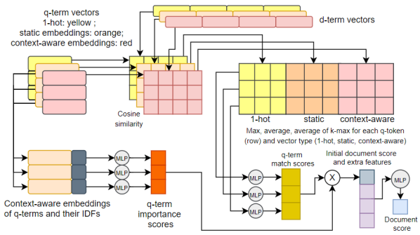
Figure 1: pdrmm for document scoring. The same model (with different trained parameters) also scores sentences in the pdrmm+pdrmm pipeline and the joint jpdrmm model (adding the layers of Fig. 2).

Each context aware q-term embedding is also concatenated with the corresponding idf score (bottom left of Fig. 1) and passed to another mlp that computes the importance of that q-term (words with low idfs may be unimportant). Let $v$ be the vector containing the $n$ match scores of the q-terms, and $u$ the vector with the corresponding $n$ importance scores (bottom right of Fig. 1). The initial relevance score of the document is $\hat{r}(q,d)=v^{T}u$. Then $\hat{r}(q,d)$ is concatenated with four extra features: z-score normalized bm25 Robertson and Zaragoza (2009); percentage of q-terms with exact match in $d$ (regular and idf weighted); percentage of q-term bigrams matched in $d$. An mlp computes the final relevance $r(q,d)$ from the 5 features.

Neural rankers typically re-rank the top $N$ documents of a conventional ir system. We use the same bm25-based ir system as McDonald et al. (2018). pdrmm is trained on triples $\left<q,d,d^{\prime}\right>$, where $d$ is a relevant document from the top $N$ of $q$, and $d^{\prime}$ is a random irrelevant document from the top $N$. We use hinge loss, requiring the relevance of $d$ to exceed that of $d^{\prime}$ by a margin.

2.2 PDRMM-based Pipelines for Document and Snippet Ranking

Brokos et al. (2018) used the ‘basic cnn’ (bcnn) of Yin et al. (2016) to score (rank) the sentences of the re-ranked top $N$ documents. The resulting pipeline, pdrmm+bcnn, had the best document and snippet results in bioasq 6, where snippets were sentences. Hence, pdrmm+bcnn is a reasonable document and snippet retrieval baseline pipeline. In another pipeline, pdrmm+pdrmm, we replace bcnn by a second instance of pdrmm that scores sentences. The second pdrmm instance is the same as when scoring documents (Fig. 1), but the input is now the query ($q$) and a single sentence ($s$). Given a triple $\left<q,d,d^{\prime}\right>$ used to train the document-scoring pdrmm, the sentence-scoring pdrmm is trained to predict the true class (relevant, irrelevant) of each sentence in $d$ and $d^{\prime}$ using cross entropy loss (with a sigmoid on $r(q,s)$). As when scoring documents, the initial relevance score $\hat{r}(q,s)$ is combined with extra features using an mlp, to obtain $r(q,s)$. The extra features are now different: character length of $q$ and $s$, number of shared tokens of $q$ and $s$ (with/without stop-words), sum of idf scores of shared tokens (with/without stop-words), sum of idf scores of shared tokens divided by sum of idf scores of q-terms, number of shared token bigrams of $q$ and $s$, bm25 score of $s$ against the sentences of $d$ and $d^{\prime}$, bm25 score of the document ($d$ or $d^{\prime}$) that contained $s$. The two pdrmm instances are trained separately.

2.3 Joint PDRMM-based Models for Document and Snippet Ranking

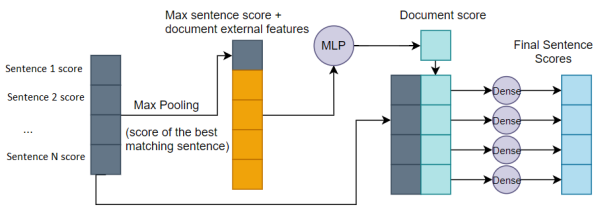
Figure 2: Final layers of jpdrmm and jbert. The input sentence scores are generated by pdrmm (Fig. 1) or bert (Fig. 3) now applied to document sentences. The document’s score is obtained from the score of its best sentence and external features, and is also used to revise the sentence scores. Training jointly minimizes document and sentence loss.

Given a document $d$ with sentences $s_{1},\dots,s_{k}$ and a query $q$, the joint document/snippet ranking version of pdrmm, called jpdrmm, processes separately each sentence $s_{i}$ of $d$, producing a relevance score $r(q,s_{i})$ per sentence, as when pdrmm scores sentences in the pdrmm+pdrmm pipeline. The highest sentence score $\max_{i}r(q,s_{i})$ is concatenated (Fig. 2) with the extra features that are used when pdrmm ranks documents, and an mlp produces the document’s score. jpdrmm then revises the sentence scores, by concatenating the score of each sentence with the document score and passing each pair of scores to a dense layer to compute a linear combination, which becomes the revised sentence score. Notice that jpdrmm is mostly based on scoring sentences, since the main goal for qa is to obtain good snippets (almost final answers). The document score is obtained from the score of the document’s best sentence (and external features), but the sentence scores are revised, once the document score has been obtained. We use sentence-sized snippets, for compatibility with bioasq, but other snippet granularities (e.g., paragraph-sized) could also be used.

jpdrmm is trained on triples $\left<q,d,d^{\prime}\right>$, where $d,d^{\prime}$ are relevant and irrelevant documents, respectively, from the top $N$ of query $q$, as in the original pdrmm; the ground truth now also indicates which sentences of the documents are relevant or irrelevant, as when training pdrmm to score sentences in pdrmm+pdrmm. We sum the hinge loss of $d$ and $d^{\prime}$ and the cross-entropy loss of each sentence. We also experiment with a jpdrmm version that uses a pre-trained bert model Devlin et al. (2019) to obtain input token embeddings (of wordpieces) instead of the more conventional pre-trained (e.g., word2vec) word embeddings that jpdrmm uses otherwise. We call it bjpdrmm if bert is fine-tuned when training jpdrmm, and bjpdrmm-nf if bert is not fine-tuned. In another variant of bjpdrmm, called bjpdrmm-adapt, the input embedding of each token is a linear combination of all the embeddings that bert produces for that token at its different Transformer layers. The weights of the linear combination are learned via backpropagation. This allows bjpdrmm-adapt to learn which bert layers it should mostly rely on when obtaining token embeddings. Previous work has reported that representations from different bert layers may be more appropriate for different tasks Rogers et al. (2020). bjpdrmm-adapt-nf is the same as bjpdrmm-adapt, but bert is not fine-tuned; the weights of the linear combination of embeddings from bert layers are still learned.

2.4 Pipelines and Joint Models Based on Ranking with BERT

The bjpdrmm model we discussed above and its variants are essentially still jpdrmm, which in turn invokes the pdrmm ranker (Fig. 1, 2); bert is used only to obtain token embeddings that are fed to jpdrmm. Instead, in this subsection we use bert as a ranker, replacing pdrmm.

For document ranking alone (when not cosidering snippets), we feed bert with pairs of questions and documents (Fig. 3). bert’s top-layer embedding of the ‘classification’ token [cls] is concatenated with external features (the same as when scoring documents with pdrmm, Section 2.1), and a dense layer again produces the document’s score. We fine-tune the entire model using triples $\left<q,d,d^{\prime}\right>$ with a hinge loss between $d$ and $d^{\prime}$, as when training pdrmm to score documents.

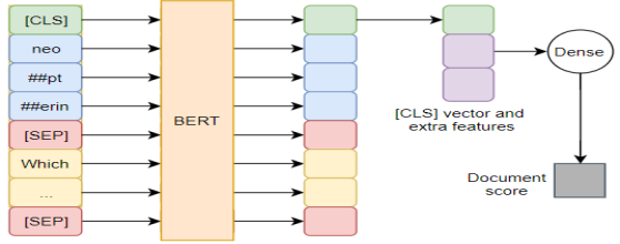
Figure 3: Document scoring with bert. The same model scores sentences in jbert (adding the layers of Fig. 2), but with an mlp replacing the final dense layer.

Our two pipelines that use bert for document ranking, bert+bcnn and bert+pdrmm, are the same as pdrmm+bcnn and pdrmm+pdrmm (Section 2.2), respectively, but use the bert ranker (Fig. 3) to score documents, instead of pdrmm. The joint jbert model is the same as jpdrmm, but uses the bert ranker (Fig. 3), now applied to sentences, instead of pdrmm (Fig. 1), to obtain the initial sentence scores. The top layers of Fig. 2 are then used, as in all joint models, to obtain the document score from the sentence scores and revise the sentence scores. Similarly to bjpdrmm, we also experimented with variations of jbert, which do not fine-tune the parameters of bert (jbert-nf), use a linear combination (with trainable weights) of the [cls] embeddings from all the bert layers (jbert-adapt), or both (jbert-adapt-nf).

2.5 BM25+BM25 Baseline Pipeline

We include a bm25+bm25 pipeline to measure the improvement of the proposed models on conventional ir engines. This pipeline uses the question as a query to the ir engine and selects the $N_{d}$ documents with the highest bm25 scores. The $N_{d}$ documents are then split into sentences and bm25 is re-computed, this time over all the sentences of the $N_{d}$ documents, to retrieve the $N_{s}$ best sentences.

3 Experiments

3.1 Data and Experimental Setup

BioASQ data and setup

Following McDonald et al. (2018) and Brokos et al. (2018), we experiment with data from bioasq Tsatsaronis et al. (2015), which provides English biomedical questions, relevant documents from medline/pubmed, and relevant snippets (sentences), prepared by biomedical experts. This is the only previous large-scale ir dataset we know of that includes both gold documents and gold snippets. We use the bioasq 7 (2019) training dataset, which contains 2,747 questions, with 11 gold documents and 14 gold snippets per question on average. We evaluate on test batches 1–5 (500 questions in total) of bioasq 7. We measure Mean Average Precision (map) Manning et al. (2008) for document and snippet retrieval, which are the official bioasq evaluation measures. The document collection contains approx. 18m articles (concatenated titles and abstracts only, discarding articles with no abstracts) from the medline/pubmed ‘baseline’ 2018 dataset. In pdrmm and bcnn, we use the biomedical word2vec embeddings of McDonald et al. (2018). We use the galago ir engine to obtain the top $N=100$ documents per query. After re-ranking, we return $N_{d}=10$ documents and $N_{s}=10$ sentences, as required by bioasq. We train using Adam Kingma and Ba (2015). Hyper-parameters were tuned on held-out validation data.

Natural Questions data and setup

Even though there was no other large-scale ir dataset providing multiple gold documents and snippets per question, we needed to test our best models on a second dataset, other than bioasq. Therefore we modified the Natural Questions dataset Kwiatkowski et al. (2019) to a format closer to bioasq’s. Each instance of Natural Questions consists of an html document of Wikipedia and a question. The answer to the question can always be found in the document as if a perfect retrieval engine were used. A short span of html source code is annotated by humans as a ‘short answer’ to the question. A longer span of html source code that includes the short answer is also annotated, as a ‘long answer’. The long answer is most commonly a paragraph of the Wikipedia page. In the original dataset, more than 300,000 questions are provided along with their corresponding Wikipedia html documents, short answer and long answer spans. We modified Natural Questions to fit the bioasq setting. From every Wikipedia html document in the original dataset, we extracted the paragraphs and indexed each paragraph separately to an ElasticSearch index, which was then used as our retrieval engine. We discarded all the tables and figures of the html documents and any question that was answered by a paragraph containing a table. For every question, we apply a query to our retrieval engine and retrieve the first $N=100$ paragraphs. We treat each paragraph as a document, similarly to the bioasq setting. For each question, the gold (correct) documents are the paragraphs (at most two per question) that were included in the long answers of the original dataset. The gold snippets are the sentences (at most two per question) that overlap with the short answers of the original dataset. We discard questions for which the retrieval engine did not manage to retrieve any of the gold paragraphs in its top 100 paragraphs. We ended up with 110,589 questions and 2,684,631 indexed paragraphs. Due to lack of computational resources, we only use 4,000 questions for training, 400 questions for development, and 400 questions for testing, but we make the entire modified Natural Questions dataset publicly available. Hyper-parameters were again tuned on held-out validation data. All other settings were as in the bioasq experiments.

3.2 Experimental Results

Method	Params	Doc. MAP (%)	Snip. MAP (%)	Doc. Recall@10(%)	Snip. Recall@10(%)
bm25 +bm25	4	6.86	4.29	48.65	4.93
pdrmm+bcnn	21.83k	7.47	5.67	52.97	12.43
pdrmm+pdrmm	11.39k	7.47	9.16	52.97	18.43
jpdrmm	5.79k	6.69	15.72	53.68	18.83
bert+bcnn	109.5M	8.79	6.07	55.73	13.05
bert+pdrmm	109.5M	8.79	9.63	55.73	19.30
bjpdrmm	88.5M	7.59	16.82	52.21	19.57
bjpdrmm-adapt	88.5M	6.93	15.70	48.77	19.38
bjpdrmm-nf	3.5M	6.84	15.77	48.81	17.95
bjpdrmm-adapt-nf	3.5M	7.42	17.35	52.12	19.66
jbert	85M	7.93	16.29	53.44	19.87
jbert-adapt	85M	7.81	15.99	52.94	19.87
jbert-nf	6.3K	7.90	15.99	52.78	19.64
jbert-adapt-nf	6.3K	7.84	16.53	53.18	19.64
Oracle	0	19.24	25.18	72.67	41.14
Sentence pdrmm	5.68K	6.39	8.73	48.60	18.57

Table 1: Parameters learned, document and snippet map on bioasq 7, test batches 1–5, before expert inspection. Systems in the 2nd (or 3rd) zone use (or not) bert. In each zone, best scores shown in bold. In the 2nd and 3rd zones, we underline the results of the best pipeline, the results of jpdrmm, and the best results of the bjpdrmm and jbert variants. The differences between the underlined map scores are statistically significant ($p\leq 0.01$).

BioASQ results

Table 1 reports document and snippet map scores on the bioasq dataset, along with the trainable parameters per method. For completeness, we also show recall at 10 scores, but we base the discussion below on map, the official measure of bioasq, which also considers the ranking of the 10 documents and snippets bioasq allows participants to return. The Oracle re-ranks the $N$ = 100 documents (or their snippets) that bm25 retrieved, moving all the relevant documents (or snippets) to the top. Sentence pdrmm is an ablation of jpdrmm without the top layers (Fig. 2); each sentence is scored using pdrmm, then each document inherits the highest score of its snippets.

pdrmm+bcnn and pdrmm+pdrmm use the same document ranker, hence the document map of these two pipelines is identical (7.47). However, pdrmm+pdrmm outperforms pdrmm+bcnn in snippet map (9.16 to 5.67), even though pdrmm has much fewer trainable parameters than bcnn, confirming that pdrmm can also score sentences and is a better sentence ranker than bcnn. pdrmm+bcnn was the best system in bioasq 6 for both documents and snippets, i.e., it is a strong baseline. Replacing pdrmm by bert for document ranking in the two pipelines (bert+bcnn and bert+pdrmm) increases the document map by 1.32 points (from 7.47 to 8.79) with a marginal increase in snippet map for bert+pdrmm (9.16 to 9.63) and a slightly larger increase for bert+bcnn (5.67 to 6.07), at the expense of a massive increase in trainable parameters due to bert (and computational cost to pre-train and fine-tune bert). We were unable to include a bert+bert pipeline, which would use a second bert ranker for sentences, with a total of approx. 220M trainable parameters, due to lack of computational resources.

The main joint models (jpdrmm, bjpdrmm, jbert) vastly outperform the pipelines in snippet extraction, the main goal for qa (obtaining 15.72, 16.82, 16.29 snippet map, respectively), though their document map is slightly lower (6.69, 7.59, 7.93) compared to the pipelines (7.47, 8.79), but still competitive. This is not surprising, since the joint models are geared towards snippet retrieval (they directly score sentences, document scores are obtained from sentence scores). Human inspection of the retrieved documents and snippets, discussed below (Table 2), reveals that the document map of jpdrmm is actually higher than that of the best pipeline (bert+pdrmm), but is penalized in Table 1 because of missing gold documents.

jpdrmm, which has the fewest parameters of all neural models and does not use bert at all, is competitive in snippet retrieval with models that employ bert. More generally, the joint models use fewer parameters than comparable pipelines (see the zones of Table 1). Not fine-tuning bert (-nf variants) leads to a further dramatic decrease in trainable parameters, at the expense of slightly lower document and snippet map (7.59 to 6.84, and 16.82 to 15.77, respectively, for bjpdrmm, and similarly for jbert). Using linear combinations of token embeddings from all bert layers (-adapt variants) harms both document and snippet map when fine-tuning bert, but is beneficial in most cases when not fine-tuning bert (-nf). The snippet map of bjpdrmm-nf increases from 15.77 to 17.35, and document map increases from 6.84 to 7.42. A similar increase is observed in the snippet map of jbert-nf (15.99 to 16.53), but map decreases (7.90 to 7.84). In the second and third result zones of Table 1, we underline the results of the best pipelines, the results of jpdrmm, and the results of the best bjpdrmm and jbert variant. In each zone and column, the differences between the underlined map scores are statistically significant ($p\leq 0.01$); we used single-tailed Approximate Randomization Dror et al. (2018), 10k iterations, randomly swapping in each iteration the rankings of 50% of queries. Removing the top layers of jpdrmm (Sentence pdrmm), clearly harms performance for both documents and snippets. The oracle scores indicate there is still scope for improvements in both documents and snippets.

BioASQ results after expert inspection

	Before expert inspection		After expert inspection
Method	Document map	Snippet map	Document map	Snippet map
bert+pdrmm	7.29	7.58	14.86	15.61
jpdrmm	5.16	12.45	16.55	21.98
bjpdrmm-nf	6.18	13.89	14.65	23.96
Best bioasq 7 competitor	n/a	n/a	13.18	14.98

Table 2: Document and snippet map (%) on bioasq 7 test batches 4 and 5 before and after post-contest expert inspection of system responses, for methods that participated in bioasq 7. We also show the results (after inspection) of the best other participants of bioasq 7 for the same batches.

	Document Retrieval			Snippet Retrieval
Method	MRR	Recall@1	Recall@2	MRR	Recall@1	Recall@2
bm25+bm25	30.18	16.50	29.75	8.19	3.75	7.13
pdrmm+pdrmm	40.33	28.25	38.50	22.86	13.75	22.75
jpdrmm	36.50	24.50	36.00	26.92	19.00	25.25

Table 3: mrr (%) and recall at top 1 and 2 (%) on the modified Natural Questions dataset.

At the end of each bioasq annual contest, the biomedical experts who prepared the questions and their gold documents and snippets inspect the responses of the participants. If any of the documents and snippets returned by the participants are judged relevant to the corresponding questions, they are added to the gold responses. This process enhances the gold responses and avoids penalizing participants for responses that are actually relevant, but had been missed by the experts in the initial gold responses. However, it is unfair to use the post-contest enhanced gold responses to compare systems that participated in the contest to systems that did not, because the latter may also return documents and snippets that are actually relevant and are not included in the gold data, but the experts do not see these responses and they are not included in the gold ones. The results of Table 1 were computed on the initial gold responses of bioasq 7, before the post-contest revision, because not all of the methods of that table participated in bioasq 7. In Table 2, we show results on the revised post-contest gold responses of bioasq 7, for those of our methods that participated in the challenge. We show results on test batches 4 and 5 only (out of 5 batches in total), because these were the only two batches were all three of our methods participated together. Each batch comprises 100 questions. We also show the best results (after inspection) of our competitors in bioasq 7, for the same batches.

A first striking observation in Table 2 is that all results improve substantially after expert inspection, i.e., all systems retrieved many relevant documents and snippets the experts had missed. Again, the two joint models (jpdrmm, bjpdrmm-nf) vastly outperform the bert+pdrmm pipeline in snippet map. As in Table 1, before expert inspection the pipeline has slightly better document map than the joint models. However, after expert inspection jpdrmm exceeds the pipeline in document map by almost two points. bjpdrmm-nf performs two points better than jpdrmm in snippet map after expert inspection, though jpdrmm performs two points better in document map. After inspection, the document map of bjpdrmm-nf is also very close to the pipeline’s. Table 2 confirms that jpdrmm is competitive with models that use bert, despite having the fewest parameters. All of our methods clearly outperformed the competition.

Natural Questions results

Table 3 reports results on the modified Natural Questions dataset. We experiment with the best pipeline and joint model of Table 1 that did not use bert (and are computationally much cheaper), i.e., pdrmm+pdrmm and jpdrmm, comparing them to the more conventional bm25+bm25 baseline. Since there are at most two relevant documents and snippets per question in this dataset, we measure Mean Reciprocal Rank (mrr) Manning et al. (2008), and Recall at top 1 and 2. Both pdrmm+pdrmm and jpdrmm clearly outperform the bm25+bm25 pipeline in both document and snippet retrieval. As in Table 1, the joint jpdrmm model outperforms the pdrmm+pdrmm pipeline in snippet retrieval, but the pipeline performs better in document retrieval. Again, this is unsurprising, since the joint models are geared towards snippet retrieval. We also note that jpdrmm uses half of the trainable parameters of pdrmm+pdrmm (Table 1). No comparison to previous work that used the original Natural Questions is possible, since the original dataset provides a single document per query (Section 3.1).

4 Related Work

Neural document ranking Guo et al. (2016); Hui et al. (2017); Pang et al. (2017); Hui et al. (2018); McDonald et al. (2018) only recently managed to improve the rankings of conventional ir; see Lin (2019) for caveats. Document or passage ranking models based on bert have also been proposed, with promising results, but most use only simplistic task-specific layers on top of bert Yang et al. (2019b); Nogueira and Cho (2019), similar to our use of bert for document scoring (Fig. 3). An exception is the work of MacAvaney et al. (2019), who explored combining elmo Peters et al. (2018) and bert Devlin et al. (2019) with complex neural ir models, namely pacrr Hui et al. (2017), drmm Guo et al. (2016), knrm Dai et al. (2018), convknrm Xiong et al. (2017), an approach that we also explored here by combining bert with pdrmm in bjpdrmm and jbert. However, we retrieve both documents and snippets, whereas MacAvaney et al. (2019) retrieve only documents.

Models that directly retrieve documents by indexing neural document representations, rather than re-ranking documents retrieved by conventional ir, have also been proposed Fan et al. (2018); Ai et al. (2018); Khattab and Zaharia (2020), but none addresses both document and snippet retrieval. Yang et al. (2019a) use bert to encode, index, and directly retrieve snippets, but do not consider documents; indexing snippets is also computationally costly. Lee et al. (2019) propose a joint model for direct snippet retrieval (and indexing) and answer span selection, again without retrieving documents.

No previous work combined document and snippet retrieval in a joint neural model. This may be due to existing datasets, which do not provide both gold documents and gold snippets, with the exception of bioasq, which is however small by today’s standards (2.7k training questions, Section 3.1). For example, Pang et al. (2017) used much larger clickthrough datasets from a Chinese search engine, as well as datasets from the 2007 and 2008 trec Million Query tracks Qin et al. (2010), but these datasets do not contain gold snippets. squad Rajpurkar et al. (2016) and squad v.2 Rajpurkar et al. (2018) provide 100k and 150k questions, respectively, but for each question they require extracting an exact answer span from a single given Wikipedia paragraph; no snippet retrieval is performed, because the relevant (paragraph-sized) snippet is given. Ahmad et al. (2019) provide modified versions of squad and Natural Questions, suitable for direct snippet retrieval, but do not consider document retrieval. SearchQA Dunn et al. (2017) provides 140k questions, along with 50 snippets per question. The web pages the snippets were extracted from, however, are not included in the dataset, only their urls, and crawling them may produce different document collections, since the contents of web pages often change, pages are removed etc. ms-marco Nguyen et al. (2016) was constructed using 1M queries extracted from Bing’s logs. For each question, the dataset includes the snippets returned by the search engine for the top-10 ranked web pages. However the gold answers to the questions are not spans of particular retrieved snippets, but were freely written by humans after reading the returned snippets. Hence, gold relevant snippets (or sentences) cannot be identified, making this dataset unsuitable for our purposes.

5 Conclusions and Future Work

Our contributions can be summarized as follows: (1) We proposed an architecture to jointly rank documents and snippets with respect to a question, two particularly important stages in qa for large document collections; our architecture can be used with any neural text relevance model. (2) We instantiated the proposed architecture using a recent neural relevance model (pdrmm) and a bert-based ranker. (3) Using biomedical data (from bioasq), we showed that the two resulting joint models (pdrmm-based and bert-based) vastly outperform the corresponding pipelines in snippet retrieval, the main goal in qa for document collections, using fewer parameters, and also remaining competitive in document retrieval. (4) We showed that the joint model (pdrmm-based) that does not use bert is competitive with bert-based models, outperforming the best bioasq 6 system; our joint models (pdrmm- and bert-based) also outperformed all bioasq 7 competitors. (5) We provide a modified version of the Natural Questions dataset, suitable for document and snippet retrieval. (6) We showed that our joint pdrmm-based model also largely outperforms the corresponding pipeline on open-domain data (Natural Questions) in snippet retrieval, even though it performs worse than the pipeline in document retrieval. (7) We showed that all the neural pipelines and joint models we considered improve the traditional bm25 ranking on both datasets. (8) We make our code publicly available.

We hope to extend our models and datasets for stage (iv), i.e., to also identify exact answer spans within snippets (paragraphs), similar to the answer spans of squad Rajpurkar et al. (2016, 2018). This would lead to a multi-granular retrieval task, where systems would have to retrieve relevant documents, relevant snippets, and exact answer spans from the relevant snippets. bioasq already includes this multi-granular task, but exact answers are provided only for factoid questions and they are freely written by humans, as in ms-marco, with similar limitations. Hence, appropriately modified versions of the bioasq datasets are needed.

Appendix

Tuning the weights of the two losses and the effect of extra features in jpdrmm

In Table 1, all joint models used the sum of the document and snippet loss ($L=L_{\textit{doc}}+L_{\textit{snip}}$). By contrast, in Table 4 we use a linear combination $L=L_{\textit{doc}}+\lambda_{\textit{snip}}L_{\textit{snip}}$ and tune the hyper-parameter $\lambda_{\textit{snip}}\in\{10,1,0.1,0.01\}$. We also try removing the extra document and/or sentence features (Fig. 1–3) to check their effect. This experiment was performed only with jpdrmm, which is one of our best joint models and computationally much cheaper than methods that employ bert. As in Table 1, we use the bioasq data, but here we perform a 10-fold cross-validation on the union of the training and development subsets. This is why the results for $\lambda_{\textit{snip}}=1$ when using both the sentence and document extra features (row 4, in italics) are slightly different than the corresponding jpdrmm results of Table 1 (6.69 and 15.72, respectively).

Sent.	Doc.		Doc.	Snip.
Extra	Extra	$\lambda_{\textit{snip}}$	MAP (%)	MAP (%)
Yes	Yes	10	6.23 $\pm$ 0.14	14.73 $\pm$ 0.32
Yes	No	10	1.20 $\pm$ 0.14	3.59 $\pm$ 0.45
No	Yes	10	1.18 $\pm$ 0.23	2.19 $\pm$ 0.29
Yes	Yes	1	6.80 $\pm$ 0.07	15.42 $\pm$ 0.23
Yes	No	1	1.35 $\pm$ 0.24	3.77 $\pm$ 0.73
No	Yes	1	7.35 $\pm$ 0.16	14.58 $\pm$ 0.88
Yes	Yes	0.1	7.85 $\pm$ 0.08	17.28 $\pm$ 0.26
Yes	No	0.1	6.77 $\pm$ 0.25	13.86 $\pm$ 1.10
No	Yes	0.1	7.59 $\pm$ 0.12	15.77 $\pm$ 0.60
Yes	Yes	0.01	7.83 $\pm$ 0.07	17.34 $\pm$ 0.37
Yes	No	0.01	6.61 $\pm$ 0.19	12.96 $\pm$ 0.29
No	Yes	0.01	7.65 $\pm$ 0.10	14.24 $\pm$ 1.63

Table 4: jpdrmm results on bioasq 7 data for tuned weights of the two losses, with and without the extra sentence and document features. The 4th row (in italics) corresponds to the jpdrmm configuration of Table 1, but the results here are slightly different, because we used a 10-fold cross-validation on the training and development data. The map scores are averaged over the 10 folds. We also report standard deviations ($\pm$).

Table 4 shows that further performance gains (6.80 to 7.85 document map, 15.42 to 17.34 snippet map) are possible by tuning the weights of the two losses. The best scores are obtained when using both the extra sentence and document features. However, the model performs reasonably well even when one of the two types of extra features is removed, with the exception of $\lambda_{\textit{snip}}=10$. The standard deviations of the map scores over the folds of the cross-validation indicate that the performance of the model is reasonably stable.

Error Analysis and Limitations

We conducted an exploratory analysis of the retrieved snippets in the two datasets. For each dataset, we used the model with the best snippet retrieval performance, i.e., jpdrmm for the modified Natural Questions (Table 3) and bjpdrmm-adapt-nf for bioasq (Table 1).

Both models struggle to retrieve the gold sentences when the answer is not explicitly mentioned in them. For example, the gold sentence for the question “What is the most famous fountain in Rome?” of the Natural Questions dataset is:

“The Trevi Fountain (Italian: Fontana di Trevi) is a fountain in the Trevi district in Rome, Italy, designed by Italian architect Nicola Salvi and completed by Giuseppe Pannini.”

Instead, the top sentence of jpdrmm is the following, which looks reasonably good, but mentions famous fountains (of a particular kind) near Rome.

“The most famous fountains of this kind were found in the Villa d’Este, at Tivoli near Rome, which featured a hillside of basins, fountains and jets of water, as well as a fountain which produced music by pouring water into a chamber, forcing air into a series of flute-like pipes.”.

To prefer the gold sentence, the model needs to know that Fontana di Trevi is also very famous, but this information is not included in the gold sentence itself, though it is included in the next sentence:

“Standing 26.3 metres (86 ft) high and 49.15 metres (161.3 ft) wide, it is the largest Baroque fountain in the city and one of the most famous fountains in the world.”

Hence, some form of multi-hop qa Yang et al. (2018); Bauer et al. (2018); Khot et al. (2019); Saxena et al. (2020) seems to be needed to combine the information that Fontana di Trevi is in Rome (explicitly mentioned in the gold sentence) with information from the next sentence and, more generally, other sentences even from different documents.

In the case of the question “What part of the body is affected by mesotheliomia?” of the bioasq dataset, the gold sentence is:

‘’Malignant pleural mesothelioma (MPM) is a hard to treat malignancy arising from the mesothelial surface of the pleura.”

Instead, the top sentence of bjpdrmm-adapt-nf is the following, which contains several words of the question, but not ‘mesothelioma’, which is the most important question term.

“For PTs specialized in acute care, geriatrics and pediatrics, the body part most commonly affected was the low back, while for PTs specialized in orthopedics and neurology, the body part most commonly affected was the neck.”

In this case, the gold sentence does not explicitly convey that the pleura is a membrane that envelops each lung of the human body and, therefore, a part of the body. Again, this additional information can be found in other sentences.

References

- Ahmad et al. (2019) Amin Ahmad, Noah Constant, Yinfei Yang, and Daniel Cer. 2019. ReQA: An evaluation for end-to-end answer retrieval models. In Proceedings of the 2nd Workshop on Machine Reading for Question Answering, pages 137–146, Hong Kong, China.
- Ai et al. (2018) Qingyao Ai, Brendan O’Connor, and W. Bruce Croft. 2018. A Neural Passage Model for Ad-hoc Document Retrieval. In Advances in Information Retrieval, Cham.
- Bauer et al. (2018) Lisa Bauer, Yicheng Wang, and Mohit Bansal. 2018. Commonsense for generative multi-hop question answering tasks. In Proceedings of the 2018 Conference on Empirical Methods in Natural Language Processing, pages 4220–4230, Brussels, Belgium.
- Brokos et al. (2018) George Brokos, Polyvios Liosis, Ryan McDonald, Dimitris Pappas, and Ion Androutsopoulos. 2018. AUEB at BioASQ 6: Document and Snippet Retrieval. In Proceedings of the 6th BioASQ Workshop, pages 30–39, Brussels, Belgium.
- Chen et al. (2017) Danqi Chen, Adam Fisch, Jason Weston, and Antoine Bordes. 2017. Reading Wikipedia to answer open-domain questions. In Proceedings of the 55th Annual Meeting of the Association for Computational Linguistics (Volume 1: Long Papers), pages 1870–1879, Vancouver, Canada.
- Cui et al. (2017) Yiming Cui, Zhipeng Chen, Si Wei, Shijin Wang, Ting Liu, and Guoping Hu. 2017. Attention-over-Attention Neural Networks for Reading Comprehension. In Proceedings of the 55th Annual Meeting of the Association for Computational Linguistics (Volume 1: Long Papers), pages 593–602, Vancouver, Canada.
- Dai et al. (2018) Zhuyun Dai, Chenyan Xiong, Jamie Callan, and Zhiyuan Liu. 2018. Convolutional neural networks for soft-matching n-grams in ad-hoc search. In Proceedings of the Eleventh ACM International Conference on Web Search and Data Mining, pages 126–134, Marina Del Rey, CA.
- Devlin et al. (2019) Jacob Devlin, Ming-Wei Chang, Kenton Lee, and Kristina Toutanova. 2019. BERT: Pre-training of Deep Bidirectional Transformers for Language Understanding. In Proceedings of the 2019 Conference of the North American Chapter of the Association for Computational Linguistics: Human Language Technologies, Volume 1 (Long and Short Papers), pages 4171–4186.
- Dror et al. (2018) Rotem Dror, Gili Baumer, Segev Shlomov, and Roi Reichart. 2018. The Hitchhiker’s Guide to Testing Statistical Significance in Natural Language Processing. In Proceedings of the 56th Annual Meeting of the ACL (Volume 1: Long Papers), pages 1383–1392.
- Dunn et al. (2017) Matthew Dunn, Levent Sagun, Mike Higgins, V. Ugur Güney, Volkan Cirik, and Kyunghyun Cho. 2017. SearchQA: A New Q&A Dataset Augmented with Context from a Search Engine. ArXiv, abs/1704.05179.
- Fan et al. (2018) Yixing Fan, Jiafeng Guo, Yanyan Lan, Jun Xu, Chengxiang Zhai, and Xueqi Cheng. 2018. Modeling Diverse Relevance Patterns in Ad-Hoc Retrieval. In The 41st International ACM SIGIR Conference on Research & Development in Information Retrieval.
- Guo et al. (2016) Jiafeng Guo, Yixing Fan, Qingyao Ai, and W. Bruce Croft. 2016. A Deep Relevance Matching Model for Ad-hoc Retrieval. In Proceedings of the 25th ACM International on Conference on Information and Knowledge Management, pages 55–64, Indianapolis, Indiana, USA.
- He et al. (2016) Kaiming He, Xiangyu Zhang, Shaoqing Ren, and Jian Sun. 2016. Deep Residual Learning for Image Recognition. In Proceedings of the IEEE conference on computer vision and pattern recognition, pages 770–778.
- Hosein et al. (2019) Stefan Hosein, Daniel Andor, and Ryan McDonald. 2019. Measuring domain portability and error propagation in biomedical QA. In Joint European Conference on Machine Learning and Knowledge Discovery in Databases, pages 686–694, Wurzburg, Germany.
- Hui et al. (2017) Kai Hui, Andrew Yates, Klaus Berberich, and Gerard de Melo. 2017. PACRR: A Position-Aware Neural IR Model for Relevance Matching. In Proceedings of the 2017 Conference on Empirical Methods in Natural Language Processing, pages 1049–1058, Copenhagen, Denmark.
- Hui et al. (2018) Kai Hui, Andrew Yates, Klaus Berberich, and Gerard de Melo. 2018. Co-PACRR: A context-aware neural IR model for ad-hoc retrieval. In Proceedings of the 11th ACM International Conference on Web Search and Data Mining, pages 279–287, Marina Del Rey, CA.
- Kadlec et al. (2016) Rudolf Kadlec, Martin Schmid, Ondrej Bajgar, and Jan Kleindienst. 2016. Text Understanding with the Attention Sum Reader Network. In Proceedings of the 54th Annual Meeting of the Association for Computational Linguistics (Volume 1: Long Papers), pages 908–918, Berlin, Germany.
- Khattab and Zaharia (2020) Omar Khattab and Matei Zaharia. 2020. ColBERT: Efficient and Effective Passage Search via Contextualized Late Interaction over BERT. ArXiv, abs/2004.12832.
- Khot et al. (2019) Tushar Khot, Ashish Sabharwal, and Peter Clark. 2019. What’s missing: A knowledge gap guided approach for multi-hop question answering. In Proceedings of the 2019 Conference on Empirical Methods in Natural Language Processing and the 9th International Joint Conference on Natural Language Processing (EMNLP-IJCNLP), pages 2814–2828, Hong Kong, China. Association for Computational Linguistics.
- Kingma and Ba (2015) Diederik P. Kingma and Jimmy Ba. 2015. Adam: A Method for Stochastic Optimization. CoRR, abs/1412.6980.
- Kwiatkowski et al. (2019) Tom Kwiatkowski, Jennimaria Palomaki, Olivia Redfield, Michael Collins, Ankur Parikh, Chris Alberti, Danielle Epstein, Illia Polosukhin, Matthew Kelcey, Jacob Devlin, Kenton Lee, Kristina N. Toutanova, Llion Jones, Ming-Wei Chang, Andrew Dai, Jakob Uszkoreit, Quoc Le, and Slav Petrov. 2019. Natural Questions: a Benchmark for Question Answering Research. Transactions of the Association of Computational Linguistics.
- Lee et al. (2018) Jinhyuk Lee, Seongjun Yun, Hyunjae Kim, Miyoung Ko, and Jaewoo Kang. 2018. Ranking paragraphs for improving answer recall in open-domain question answering. In Proceedings of the 2018 Conference on Empirical Methods in Natural Language Processing, pages 565–569, Brussels, Belgium. Association for Computational Linguistics.
- Lee et al. (2019) Kenton Lee, Ming-Wei Chang, and Kristina Toutanova. 2019. Latent retrieval for weakly supervised open domain question answering. In Proceedings of the 57th Annual Meeting of the Association for Computational Linguistics, pages 6086–6096, Florence, Italy.
- Lin (2019) Jimmy Lin. 2019. The Neural Hype and Comparisons Against Weak Baselines. SIGIR Forum, 52(2):40–51.
- MacAvaney et al. (2019) Sean MacAvaney, Andrew Yates, Arman Cohan, and Nazli Goharian. 2019. CEDR: Contextualized Embeddings for Document Ranking. CoRR, abs/1904.07094.
- Mackenzie et al. (2020) Joel Mackenzie, Zhuyun Dai, Luke Gallagher, and Jamie Callan. 2020. Efficiency Implications of Term Weighting for Passage Retrieval, page 1821–1824. Association for Computing Machinery, New York, NY, USA.
- Manning et al. (2008) Christopher D. Manning, Prabhakar Raghavan, and Hinrich Schütze. 2008. Introduction to Information Retrieval. Cambridge University Press.
- McDonald et al. (2018) Ryan McDonald, George Brokos, and Ion Androutsopoulos. 2018. Deep Relevance Ranking Using Enhanced Document-Query Interactions. In Proceedings of the 2018 Conference on Empirical Methods in Natural Language Processing, pages 1849–1860, Brussels, Belgium.
- Mitra and Craswell (2018) Bhaskar Mitra and Nick Craswell. 2018. An Introduction to Neural Information Retrieval. Now Publishers.
- Nguyen et al. (2016) Tri Nguyen, Mir Rosenberg, Xia Song, Jianfeng Gao, Saurabh Tiwary, Rangan Majumder, and Li Deng. 2016. MS MARCO: A Human Generated MAchine Reading COmprehension Dataset. CoRR, abs/1611.09268.
- Nogueira and Cho (2019) Rodrigo Nogueira and Kyunghyun Cho. 2019. Passage Re-ranking with BERT. CoRR, abs/1901.04085.
- Pandey et al. (2019) S. Pandey, I. Mathur, and N. Joshi. 2019. Information retrieval ranking using machine learning techniques. In 2019 Amity International Conference on Artificial Intelligence (AICAI), pages 86–92.
- Pang et al. (2017) Liang Pang, Yanyan Lan, Jiafeng Guo, Jun Xu, Jingfang Xu, and Xueqi Cheng. 2017. DeepRank: A New Deep Architecture for Relevance Ranking in Information Retrieval. In Proceedings of the 2017 ACM on Conference on Information and Knowledge Management.
- Peters et al. (2018) Matthew Peters, Mark Neumann, Mohit Iyyer, Matt Gardner, Christopher Clark, Kenton Lee, and Luke Zettlemoyer. 2018. Deep Contextualized Word Representations. In Proceedings of the 2018 Conference of the North American Chapter of the Association for Computational Linguistics: Human Language Technologies, pages 2227–2237, New Orleans, Louisiana.
- Qin et al. (2010) Tao Qin, Tie-Yan Liu, Jun Xu, and Hang Li. 2010. Letor: A benchmark collection for research on learning to rank for information retrieval. Inf. Retrieval.
- Rajpurkar et al. (2018) Pranav Rajpurkar, Robin Jia, and Percy Liang. 2018. Know what you don’t know: Unanswerable questions for SQuAD. In Proceedings of the 56th Annual Meeting of the Association for Computational Linguistics (Volume 2: Short Papers), pages 784–789, Melbourne, Australia.
- Rajpurkar et al. (2016) Pranav Rajpurkar, Jian Zhang, Konstantin Lopyrev, and Percy Liang. 2016. SQuAD: 100,000+ questions for machine comprehension of text. In Proceedings of the 2016 Conference on Empirical Methods in Natural Language Processing, pages 2383–2392, Austin, Texas.
- Robertson and Zaragoza (2009) Stephen Robertson and Hugo Zaragoza. 2009. The probabilistic relevance framework: BM25 and beyond. Foundations and Trends in Information Retrieval, 3(4):333–389.
- Rogers et al. (2020) Anna Rogers, Olga Kovaleva, and Anna Rumshisky. 2020. A primer in BERTology: What we know about how BERT works. Transactions of the Association for Computational Linguistics, 8.
- Saxena et al. (2020) Apoorv Saxena, Aditay Tripathi, and Partha Talukdar. 2020. Improving multi-hop question answering over knowledge graphs using knowledge base embeddings. In Proceedings of the 58th Annual Meeting of the Association for Computational Linguistics, pages 4498–4507, Online.
- Sekulić et al. (2020) Ivan Sekulić, Amir Soleimani, Mohammad Aliannejadi, and Fabio Crestani. 2020. Longformer for MS MARCO Document Re-ranking Task. ArXiv, abs/2009.09392.
- Sultan et al. (2016) Md Arafat Sultan, Vittorio Castelli, and Radu Florian. 2016. A Joint Model for Answer Sentence Ranking and Answer Extraction. Transactions of the Association for Computational Linguistics, 4:113–125.
- Tsatsaronis et al. (2015) G. Tsatsaronis, G. Balikas, P. Malakasiotis, I. Partalas, M. Zschunke, M.R. Alvers, D. Weissenborn, A. Krithara, S. Petridis, D. Polychronopoulos, Y. Almirantis, J. Pavlopoulos, N. Baskiotis, P. Gallinari, T. Artieres, A. Ngonga, N. Heino, E. Gaussier, L. Barrio-Alvers, M. Schroeder, I. Androutsopoulos, and G. Paliouras. 2015. An overview of the BioASQ Large-Scale Biomedical Semantic Indexing and Question Answering Competition. BMC Bioinformatics, 16(138).
- Voorhees (2001) Ellen M. Voorhees. 2001. The TREC question answering track. Natural Language Engineering, 7(4):361–378.
- Xiong et al. (2017) Chenyan Xiong, Zhuyun Dai, Jamie Callan, Zhiyuan Liu, and Russell Power. 2017. End-to-end neural ad-hoc ranking with kernel pooling. In Proceedings of the 40th International ACM SIGIR Conference on Research and Development in Information Retrieval, pages 55–64, Shinjuku, Tokyo, Japan.
- Xu et al. (2019) Peng Xu, Xiaofei Ma, Ramesh Nallapati, and Bing Xiang. 2019. Passage Ranking with Weak Supervsion. arxiv.
- Yang et al. (2019a) Wei Yang, Yaxiong Xie, Aileen Lin, Xingyu Li, Luchen Tan, Kun Xiong, Ming Li, and Jimmy Lin. 2019a. End-to-End open-Domain Question Answering with BERTserini. CoRR, abs/1902.01718.
- Yang et al. (2019b) Wei Yang, Haotian Zhang, and Jimmy Lin. 2019b. Simple Applications of BERT for Ad Hoc Document Retrieval. CoRR, abs/1903.10972.
- Yang et al. (2018) Zhilin Yang, Peng Qi, Saizheng Zhang, Yoshua Bengio, William Cohen, Ruslan Salakhutdinov, and Christopher D. Manning. 2018. HotpotQA: A dataset for diverse, explainable multi-hop question answering. In Proceedings of the 2018 Conference on Empirical Methods in Natural Language Processing, pages 2369–2380, Brussels, Belgium.
- Yang et al. (2016) Zichao Yang, Diyi Yang, Chris Dyer, Xiaodong He, Alex Smola, and Eduard Hovy. 2016. Hierarchical Attention Networks for Document Classification. In Proceedings of the 2016 Conference of the North American Chapter of the Association for Computational Linguistics: Human Language Technologies.
- Yin et al. (2016) Wenpeng Yin, Hinrich Schütze, Bing Xiang, and Bowen Zhou. 2016. ABCNN: Attention-based convolutional neural network for modeling sentence pairs. Transactions of the Association for Computational Linguistics, 4.
- Zhang et al. (2020) Zhuosheng Zhang, Jun jie Yang, and Hai Zhao. 2020. Retrospective reader for machine reading comprehension. ArXiv.