Variational principles and finite element Bloch analysis in couple stress elastodynamics

Abstract

We address the numerical simulation of periodic solids (phononic crystals) within the framework of couple stress elasticity. The additional terms in the elastic potential energy lead to dispersive behavior in shear waves, even in the absence of material periodicity. To study the bulk waves in these materials, we establish an action principle in the frequency domain and present a finite element formulation for the wave propagation problem related to couple stress theory subject to an extended set of Bloch-periodic boundary conditions. A major difference from the traditional finite element formulation for phononic crystals is the appearance of higher-order derivatives. We solve this problem with the use of a Lagrange-multiplier approach. After presenting the variational principle and general finite element treatment, we particularize it to the problem of finding dispersion relations in elastic bodies with periodic material properties. The resulting implementation is used to determine the dispersion curves for homogeneous and porous couple stress solids, in which the latter is found to exhibit an interesting bandgap structure.

Keywords: Micromechanics, phononic crystals, couple stress elasticity, wave propagation, dispersive media, metamaterials.

1 Introduction

There has been significant interest, especially in recent years, to develop spatially periodic band gap materials and structures, based upon Floquet-Bloch theory (Floquet, 1883; Bloch, 1929). Recent developments in the field of architectured materials aimed at achieving novel mechanical properties often rely on enhancements that include effects neglected by classical theories. Continuum models with local microstructural interactions have become increasingly popular after the advance and growth in the field of metamaterials, as summarized in the monograph by Banerjee (2011). A family of models that has regained popularity in the last few years is the so-called Cosserat-based theories, which are mainly founded on the formulation by Cosserat and Cosserat (1909). In a wide sense, these material models consider microstructural effects through a generalization of Cauchy’s postulate to include additional mechanical interactions involving couples per unit surface or couple-stresses. In the present work, we focus on a pure continuum mechanics representation by widening the modeling capabilities of consistent-couple stress theory (C-CST), originally formulated in Hadjesfandiari and Dargush (2011). In particular, we establish for the first time a principle of stationary correlated action for the corresponding reduced wave equation of elastodynamics and extend the theory to spatially periodic materials, thus providing an objective physical basis to characterize material through its dispersive behaviour.

The entire family of Cosserat elasticity models depart from the classical Cauchy models in the consideration of microstructural effects, which are unavoidably expected to occur once the specimen dimensions become comparable to the material microstructural features. These effects cannot be addressed in classical theories. On the other hand, microstructural effects are introduced through the extension of dynamic and kinematic descriptors from classical continuum mechanics on a range of alternative models. Voigt (1910) was probably the first to postulate a model with asymmetric mechanical interactions in terms of couple-stresses: the interaction between two material points in this continuum encompassed couples per unit contact surface in addition to the classical Cauchy forces per unit surface. In a landmark contribution, the Cosserat brothers (Cosserat and Cosserat, 1909) formulated a mathematical theory involving couple-stresses in which new kinematic variables were introduced in the form independent micro-rotations. Various later extensions from these theories were also developed by Eringen (1966); Nowacki (1986); Mindlin (1964); Eringen and Suhubi (1964) in micropolar, microstretch and micromorphic theories. Alongside, a different branch of developments resulted in a set of couple stress theories in the work by Toupin (1962), Mindlin and Tiersten (1962) and Koiter (1964), who used the gradients of the true continuum rotation field to provide the required kinematic enrichment.

Developments from Hadjesfandiari and Dargush (2011) have resulted in a consistent version of the models by Toupin (1962), Mindlin and Tiersten (1962) and Koiter (1964) in terms of couple-stresses. The consistency of this model is reflected in the determinacy of all the force-stress and couple-stress components, the identification of the necessary and sufficient set of natural and essential boundary conditions and the elimination of redundant force components. An approach for evaluating the usefulness and robustness of a continuum mechanics model is through the determination of its band structure in terms of its dispersion relationships. These indicate the kinematic response of the material through an identification of the wave propagation modes that can exist within the model and the frequency dependency of the group and phase velocities of these potential waves. An effective technique, relying on the assumption of spatial periodicity, is based on Bloch’s theorem from solid state physics (Brillouin, 1953), where the problem of finding the band structure reduces to solving a series of generalized eigenvalue problems for a variation of the wave vector in the reciprocal space. In the case of the C-CST model, this problem poses several computational challenges. First, since the enriched kinematic variables are now curvatures, corresponding to particular second order gradients of the displacement field, the displacement-based finite element formulation now would require $C^{1}$ interelement continuity. As shown by Darrall et al. (2014), this numerical issue can be resolved by introducing Lagrange multiplier techniques, however it is not obvious how to incorporate these within Bloch analysis. Second, as a result of enforcing the kinematic constraint in terms of Lagrange multipliers, the computational framework lacks inertial components associated with the rotational interactions. Since there is only a mass matrix associated with the translational degrees of freedom, special attention is needed in solving the eigenproblem. Both of these issues are resolved in the present work.

The characterization of the bulk properties of periodic materials is commonly done finding the band structure or dispersion relations (Hussein et al., 2014). Commonly, this band structure is obtained using a numerical method such as the Boundary Element Method (Li et al., 2013a, b), the Finite Difference Method (Tanaka et al., 2000; Su et al., 2010; Isakari et al., 2016), the Finite Element Method (Langlet et al., 1995; Guarín-Zapata and Gomez, 2015; Valencia et al., 2019; Mazzotti et al., 2019; Guarín-Zapata et al., 2020; Chin et al., 2021), or the Plane Wave Expansions (Cao et al., 2004; Xie et al., 2017; Dal Poggetto and Serpa, 2020). We favor the use of the Finite Element Method because of its maturity and versatily to represent arbitrary geometries and boundary conditions. In this work, we find the dispersion relations modeling a single unit cell of the material and using Bloch’s theorem. There have been few works on periodic materials involving generalized continua and these have been related to micropolar elasticity (Zhang et al., 2018; Guarín-Zapata et al., 2020). To the best of our knowledge, this is the first work using a higher-order elasticity model for phononic crystals.

Here we establish a new variational principle in the temporal frequency domain for reduced couple stress elastodynamics and then extend the finite element algorithm from Darrall et al. (2014) to the case of spatially periodic material cells with Bloch boundary conditions. We examine first the closed form dispersion relationships for the homogeneous version of the model. This homogeneous model already involves micromechanical effects through a length scale material parameter, however additional effects can be considered in terms of explicit representations of geometric features at the fundamental material cell level. We then formulate a variational statement together with the imposition of an extended version of the usual Bloch periodic boundary conditions that satisfies Hermiticity and positive definiteness for C-CST. Subsequently, this statement is modified by introducing an artificial independent rotation field tied to the continuum displacement field through the enforcement of a Lagrange multiplier field that is shown to equal the skew-symmetric part of the force-stresses. The resulting numerical framework is tested by comparing its results with those obtained in closed form for the homogeneous case and by applying it to a porous periodic material cell design, which displays interesting bandgap behavior that has not been resported previously.

2 Governing equations

2.1 Forces and moments in the C-CST solid

The fundamental signature of the extended continuum model considered in this work is the presence of rotational mechanical interaction, in addition to the classical translational interaction between material points in the continuum. Following a generalized Cauchy’s postulate (Mindlin and Tiersten, 1962; Koiter, 1964) we define force and couple traction vectors $t_{i}^{(\hat{n})}$ and $m_{i}^{(\hat{n})}$ respectively as

$$t_{i}^{(\hat{n})}=\lim_{\Delta S(\hat{n})\rightarrow 0}\frac{\Delta R_{i}}{\Delta S(\hat{n})}$$ (1a)

$$m_{i}^{(\hat{n})}=\lim_{\Delta S(\hat{n})\rightarrow 0}\frac{\Delta M_{i}}{\Delta S(\hat{n})}\,,$$ (1b)

and where $\Delta S(\hat{n})$ is a small element of area oriented with unit normal $\hat{n}$ while $\Delta R_{i}$ and $\Delta M_{i}$ are the resultant force and couple moment, respectively. However, only the tangential components of $m_{i}^{(\hat{n})}$ exist as independent bending couple tractions (fig. 1).

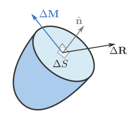
Figure 1: In the C-CST model mechanical effects are described through linear and rotational interactions in terms of resultant forces and moments at the material point. These resultants act on the surface element $\Delta S$ over a plane whose unit outward normal is $\hat{n}$.

Note that while the force-tractions vector $t_{i}^{(\hat{n})}$ is a polar vector, the couple-tractions vector $m_{i}^{(\hat{n})}$ is an axial vector. Force-tractions and couple-tractions are also described by projections of the non-symmetric force-stress tensor $\sigma_{ij}$ and the couple-stress $\mu_{ij}$ tensors according to:

$$t_{i}^{(\hat{n})}=\sigma_{ji}n_{j}\,,$$ (2a)

$$m_{i}^{(\hat{n})}=\mu_{ji}n_{j}=\epsilon_{ijk}\mu_{k}n_{j}\,,$$ (2b)

where $\mu_{ij}$ is skew-symmetric. Thus, $\mu_{ij}=-\mu_{ji}$ and the couple-stress tensor can be written as a polar vector with

$$\mu_{k}=\frac{1}{2}\epsilon_{kji}\mu_{ji}\,,$$

where $\epsilon_{ijk}$ is the Levi-Civita permutation symbol leading to the last form in (2b), which clearly shows that $m_{i}^{(\hat{n})}$ is tangential to the surface.

Consideration of the linear and angular balance equations for an arbitrary part of the material continuum of volume $V$, bounded by external surface $S$ leads to the following force-stress and couple-stress equilibrium equations for the C-CST model:

$$\begin{split}&\sigma_{ji,j}+f_{i}=\rho\ddot{u}_{i}\,,\\ &\mu_{ji,j}+\epsilon_{ijk}\sigma_{jk}=0\,,\end{split}$$ (3)

where $f_{i}$ are forces per unit volume, and $\rho$ is the mass density. Notice that, in contrast to micropolar models (Guarín-Zapata et al., 2020) where there is a rotational inertial density and a body couple term, in this model the balance equations already include those contributions. This particular aspect of the C-CST model is discussed in the original paper by Hadjesfandiari and Dargush (2011) where it is also proved that from

$$\epsilon_{ijk}(\mu_{k,j}+\sigma_{jk})=0\,,$$ (4)

it follows that $\mu_{k,j}+\sigma_{jk}$ is symmetric and as a result its skew-symmetric part is zero leading to

$$\sigma_{[ji]}=-\mu_{[i,j]}\,.$$

This gives the skew-symmetric part of the force-stress tensor in terms of the couple-stress vector, which also can be described by its dual vector representation

$$s_{i}=\frac{1}{2}\epsilon_{ijk}\mu_{k,j}\,.$$

2.2 Kinematics and constitutive relations

In the linear C-CST model, kinematics is described by the classical infinitesimal strain ($e_{ij}$) and rotation ($\theta_{ij}$) tensors

$$e_{ij}=\frac{1}{2}(u_{i,j}+u_{j,i})\,,$$ (5a)

$$\theta_{ij}=\frac{1}{2}(u_{i,j}-u_{j,i})\,,$$ (5b)

and by the mean curvature tensor

$$\kappa_{ij}=\frac{1}{2}(\theta_{i,j}-\theta_{j,i})\,,$$ (6)

where

$$\theta_{i}=\frac{1}{2}\epsilon_{ijk}\theta_{kj}\,.$$

Equation (6) can also be written in polar form, as an engineering curvature vector (Darrall et al., 2014)

$$\kappa_{i}=\epsilon_{ijk}\theta_{j,k}=\frac{1}{2}(u_{i,kk}-u_{k,ik})$$ (7)

since

$$\kappa_{i}=\epsilon_{ijk}\kappa_{jk}\,.$$

For a linear elastic centrosymmetric C-CST continuum, the constitutive equations can be written as

$$\begin{split}&\sigma_{(ij)}=C_{ijkl}e_{kl}\,,\\ &\mu_{i}=D_{ij}\kappa_{j}\,,\end{split}$$ (8)

where $C_{ijjkl}$ is the stiffness tensor as in classical (anisotropic) elasticity, and $D_{ij}$ is an additional material tensor that accounts for couple-stress effects. In the expressions above, parentheses as subindices are used to indicate the symmetric part of the tensor. In the case of a linear isotropic elastic C-CST continuum,

$$\begin{split}&C_{ijkl}=\lambda\delta_{ij}\delta_{kl}+\mu(\delta_{ik}\delta_{jl}+\delta_{il}\delta_{jk}),\\ &D_{ij}=4\eta\delta_{ij},\end{split}$$ (9)

where $\mu$ and $\lambda$ are the Lamé parameters as in classical elasticity, while $\eta$ is the additional material coefficient that accounts for couple-stress effects. Then, the constitutive equations for isotropy can be simplified to

$$\begin{split}&\sigma_{(ij)}=\lambda e_{kk}\delta_{ij}+2\mu e_{ij}\,,\\ &\mu_{i}=4\eta\kappa_{i}\,.\end{split}$$ (10)

2.3 Displacement equations of motion

At this point it may be convenient to alternate between index and explicit vector notation. In the latter, the gradient operator reads $\nabla=\frac{\partial}{\partial x_{i}}$ in Cartesian coordinates. In these terms, the time domain displacement equations of motion are obtained after using the constitutive relations (10) in the equilibrium equations (3) yielding

$$(\lambda+2\mu)\nabla(\nabla\cdot\mathbf{u})-\mu\nabla\times\nabla\times\mathbf{u}+\eta\nabla^{2}\nabla\times\nabla\times\mathbf{u}=\rho\ddot{\mathbf{u}}\,.$$ (11)

Defining the phase/group speed for the longitudinal (P) wave $c_{1}$ (which is not dispersive), the low-frequency ($k\rightarrow 0$) phase/group speed for the transverse wave (S) $c_{2}$ (which is dispersive) and the intrinsic material length scale parameter $l$ (which is not present in classical elasticity), such that

$$c_{1}^{2}=\frac{\lambda+2\mu}{\rho}\,,\qquad c_{2}^{2}=\frac{\mu}{\rho}\,,\qquad l^{2}=\frac{\eta}{\mu}\,,$$ (12)

allows us to write (11) in the form

$$c_{1}^{2}\nabla(\nabla\cdot\mathbf{u})-c_{2}^{2}(1-l^{2}\nabla^{2})\nabla\times\nabla\times\mathbf{u}=\ddot{\mathbf{u}}\,.$$ (13)

2.4 Dispersion relations for unbounded domains

Using a Helmholtz decomposition, the displacement field can be written in terms of the scalar and vector potentials $\varphi$ and $\mathbf{H}$ (Arfken et al., 2005) as

$$\mathbf{u}=\nabla\varphi+\nabla\times\mathbf{H}\,,\quad\nabla\cdot\mathbf{H}=0\,,$$

and replacing this in (13) gives the following set of uncoupled wave equations

$$c_{1}^{2}\nabla^{2}\varphi=\ddot{\varphi}\,,$$ (14)

$$c_{2}^{2}(1-l^{2}\nabla^{2})\mathbf{H}=\ddot{\mathbf{H}}\,,$$ (15)

where it is observed that the equation for the rotational potential follows a higher-order wave equation that is inherently dispersive. This becomes evident after assuming a solution of the form $\mathbf{u}=\mathbf{\tilde{u}}e^{ikx-i\omega t}$ which gives the dispersion relations

$$\omega_{P}^{2}=c_{1}^{2}k^{2}\,,$$ (16)

$$\omega_{S}^{2}=c_{2}^{2}k^{2}(1+k^{2}l^{2})\,.$$ (17)

Solving the above for $k$, we have in each case

$$k_{P}^{2} =\frac{\omega^{2}}{c_{1}^{2}}\,, k_{S}^{2} =\frac{1}{2l^{2}}\left[\pm\sqrt{1+\frac{4\omega^{2}l^{2}}{c_{2}^{2}}}-1\right]\,.$$

Noticing that the quantity inside the square root is always greater than 1 indicates that we should consider only the positive root, while the negative root corresponds to an evanescent wave that should arise under certain boundary conditions. The phase and group speeds are now given by

$$v_{P} =c_{1}\,, g_{P} =c_{1}\,,$$ (18)

$$v_{S}(k) =c_{2}\sqrt{1+k^{2}l^{2}}\,, g_{S} =c_{2}\frac{1+2k^{2}l^{2}}{\sqrt{1+k^{2}l^{2}}}\,.$$

Taking the low and high frequency limits $k\rightarrow 0$ and $k\rightarrow\infty$ gives

$$\lim_{k\rightarrow 0}v_{S}=\lim_{k\rightarrow 0}g_{S}=c_{2}\,,$$

$$\lim_{k\rightarrow\infty}v_{S}=\lim_{k\rightarrow\infty}g_{S}\rightarrow\infty\,,$$

which shows how the speed of energy flow increases with frequency. All of these relations are displayed in fig. 2.

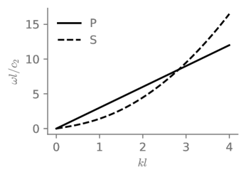
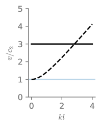
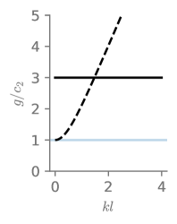
Figure 2: Dispersion relations for a homogeneous C-CST material with properties: $\rho=1\times 10^{5}$, $\lambda=2.8\times 10^{10}$, $\eta=1.62\times 10^{9}$, $\mu=4\times 10^{9}$. The plot on the left shows the frequency-wave number relation for the non-dispersive P-wave (continuous line) and the dispersive SV (dashed lines). The plots in the middle and right part of the figure show the phase and group speeds for the dispersive modes.

2.5 Frequency domain equations

Bloch analysis considering spatial periodicity of the material is naturally conducted in the Fourier domain, involving both the temporal frequencies and spatial wave numbers. After performing a Fourier transform of the linear and angular momentum equations (3) to the temporal frequency domain, these become

$$\begin{split}&\tilde{\sigma}_{ji,j}+\tilde{f}_{i}=-\rho\omega^{2}\tilde{u}_{i}\,,\\ &\tilde{\mu}_{ji,j}+\epsilon_{ijk}\tilde{\sigma}_{jk}=0\,,\end{split}$$ (19)

where the superposed tilde denotes a complex Fourier amplitude.

After introducing the constitutive equations (8) for centrosymmetric materials into (19) and then combining the angular momentum and linear momentum balance laws into a single set in terms of displacement, one finds:

$$(C_{ijkl}\tilde{u}_{k,l})_{,j}+\frac{1}{4}\epsilon_{pij}\epsilon_{pmn}\{D_{nk}(\tilde{u}_{k,ll}-\tilde{u}_{l,kl})\}_{,mj}+f_{i}=-\rho\omega^{2}\tilde{u}_{i}$$ (20)

Substituting (9) and (12) for isotropic materials into (20) provides the corresponding Fourier domain reduced wave equations in the absence of body forces, which can be written

$$c_{1}^{2}\nabla(\nabla\cdot\mathbf{\tilde{u}})-c_{2}^{2}(1-l^{2}\nabla^{2})\nabla\times\nabla\times\mathbf{\tilde{u}}=-\omega^{2}\mathbf{\tilde{u}}\,.$$ (21)

Notice that (21) is the temporal Fourier transform of (13).

3 Variational principles

We will describe next a variational formulation for the elastodynamic C-CST model. An inherent complexity is the presence of second order displacement gradients arising in the curvatures (7), which requires $C^{1}$ continuity of the displacement field.

Let us consider a volume $V$ with boundary $S$, having specified body forces $f_{i}$, force-tractions $t_{i}$, and couple-tractions $m_{i}$ (see fig. 3). The boundary $S$ is split into different segments, where $S_{u}$ represents the portion of $S$ with specified displacements, $S_{t}$ represents the surface with prescribed tractions, $S_{\theta}$ represents the segment with enforced rotations, and $S_{m}$ the boundary with prescribed couple-tractions. Additionally, $S=S_{u}\cup S_{t}=S_{\theta}\cup S_{m}$ and $S_{u}\cap S_{t}=S_{\theta}\cap S_{m}=\emptyset$. In general, $S_{u}$ and $S_{t}$ might overlap with $S_{\theta}$ and $S_{m}$. This is an important aspect of the C-CST model that is relevant in the solution of boundary value problems, as we shall see later.

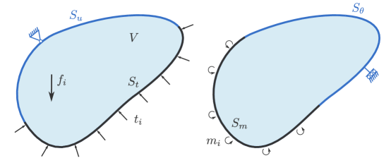
Figure 3: Schematic representation of the domain and boundary conditions for the C-CST model.

We begin with the following couple stress elastodynamic action functional in the frequency domain, as an extension of the elastostatic formulations introduced by Hadjesfandiari and Dargush (2011) and Darrall et al. (2014):

$$\mathcal{A}[u;\omega]=\mathcal{U}[u;\omega]+\mathcal{T}[u;\omega]+\mathcal{V}[u;\omega],$$ (22)

Here, and in the remainder of this paper, the superposed tilde has been suppressed for notational convenience. Meanwhile, the elastic, kinetic and applied load actions can be written in explicit form, respectively, as

$$\mathcal{U}[u;\omega]=\frac{1}{2}\int\limits_{V}e_{ij}^{*}C_{ijkl}e_{kl}\differential{V}+\frac{1}{2}\int\limits_{V}\kappa_{i}^{*}D_{ij}\kappa_{j}\differential{V},$$ (23)

$$\mathcal{T}[u;\omega]=-\frac{\omega^{2}}{2}\int\limits_{V}u_{i}^{*}\rho u_{i}\differential{V},$$ (24)

$$\mathcal{V}[u;\omega]=-\int\limits_{V}u_{i}^{*}f_{i}\differential{V}-\int\limits_{S_{t}}u_{i}^{*}t_{i}^{(\hat{n})}\differential{S}-\int\limits_{S_{m}}\theta_{i}^{*}m_{i}^{(\hat{n})}\differential{S}.$$ (25)

with the asterisk denoting complex conjugate.

The stationarity of this action becomes

$$\delta\mathcal{A}[u;\omega]=\delta\mathcal{U}[u;\omega]+\delta\mathcal{T}[u;\omega]+\delta\mathcal{V}[u,\omega])=0,$$ (26)

or

$$\begin{split}&\delta\mathcal{A}[u;\omega]=\int\limits_{V}\delta e_{ij}^{*}C_{ijkl}e_{kl}\differential{V}+\int\limits_{V}\delta\kappa_{i}^{*}D_{ij}\kappa_{j}\differential{V}-\omega^{2}\int\limits_{V}\delta u_{i}^{*}\rho u_{i}\differential{V}\\ &-\int\limits_{V}\delta u_{i}^{*}f_{i}\differential{V}-\int\limits_{S_{t}}\delta u_{i}^{*}t_{i}^{(\hat{n})}\differential{S}-\int\limits_{S_{m}}\delta\theta_{i}^{*}m_{i}^{(\hat{n})}\differential{S}=0,\,\end{split}$$ (27)

which can serve as the weak form for a finite element formulation in reduced elastodynamics. With the appearance of mean curvature in (27), this would require $C^{1}$ spatial continuity of displacements $u_{i}$.

Next, let us derive the Euler-Lagrange equations associated with the functional $\mathcal{A}[u;\omega]$. Starting from the first variation in (27), we repeatedly apply integration-by-parts operations and the divergence theorem to shift all of the spatial derivatives from the variations to the true fields. This leads to the following statement:

$$\begin{split}&\int\limits_{V}\delta u_{i}^{*}[(C_{ijkl}u_{k,l})_{,j}+\frac{1}{4}\epsilon_{pij}\epsilon_{pmn}\{D_{nk}(u_{k,ll}-u_{l,kl})\}_{,mj}+f_{i}+\rho\omega^{2}u_{i}]\differential{V}\\ &+\int\limits_{S_{t}}\delta u_{i}^{*}[t_{i}^{(\hat{n})}-\sigma_{ji}n_{j}]\differential{S}\\ &+\int\limits_{S_{m}}\delta\theta_{i}^{*}[m_{i}^{(\hat{n})}-\epsilon_{ijk}\mu_{k}n_{j}]\differential{S}=0.\,\end{split}$$ (28)

For arbitrary variations, each set of terms inside the square brackets must be zero. Thus, the Euler-Lagrange equations can be written:

$$(C_{ijkl}u_{k,l})_{,j}+\frac{1}{4}\epsilon_{pij}\epsilon_{pmn}\{D_{nk}(u_{k,ll}-u_{l,kl})\}_{,mj}+f_{i}=-\rho\omega^{2}u_{i}\quad{\rm in}\ V\\$$ (29)

$$\begin{split}&t_{i}^{(\hat{n})}=\sigma_{ji}n_{j}\quad{\rm on}\ S_{t}\\ &m_{i}^{(\hat{n})}=\epsilon_{ijk}\mu_{k}n_{j}\quad{\rm on}\ S_{m}\,\end{split}$$ (30)

Notice that (29) are the reduced wave equations from (20), while (30) represent the corresponding natural boundary conditions for C-CST. In the isotropic case, substituting (9) into (29) produces

$$c_{1}^{2}u_{j,ji}-c_{2}^{2}\epsilon_{ijk}\epsilon_{kmn}(u_{n,mj}-l^{2}u_{n,mjll})+f_{i}=-\omega^{2}u_{i}\quad{\rm in}\ V$$ (31)

which is the equivalent of (21) in index notation.

Performing an inverse Fourier transform of individual terms in (22)-(25) back to the time domain, one finds

$$\mathcal{F}^{-1}[u^{*}v]=(u\star v)(t)$$ (32)

where the $\star$ operator denotes correlation over time, such that

$$(u\star v)(t)=\int_{-\infty}^{\infty}u(\tau)v(t+\tau)d\tau.$$ (33)

Consequently, we have established the following stationary Principle of Correlated Action for couple stress elastodynamics: Of all the possible displacement fields in $V$ that satisfy the frequency domain kinematic boundary conditions on $S_{u}$ and $S_{\theta}$, the one that renders the action $\mathcal{A}[u;\omega]$ in (22) stationary corresponds to the solution of the reduced wave equations (29) and traction boundary conditions (30).

We should emphasize that this stationary Principle of Correlated Action also holds for classical theory, if one neglects contributions from mean curvature and moment tractions. Thus, the classical correlated action for reduced elastodynamics can be written:

$$\begin{split}&\mathcal{A}_{\rm cl}[u;\omega]=\frac{1}{2}\int\limits_{V}e_{ij}^{*}C_{ijkl}e_{kl}\differential{V}-\frac{\omega^{2}}{2}\int\limits_{V}u_{i}^{*}\rho u_{i}\differential{V}\\ &\qquad\qquad-\int\limits_{V}u_{i}^{*}f_{i}\differential{V}-\int\limits_{S_{t}}u_{i}^{*}t_{i}^{(\hat{n})}\differential{S}.\,\end{split}$$ (34)

4 Response of Periodic Materials

This section summarizes the most relevant theoretical aspects for the numerical analysis of periodic materials. An in-depth treatment of the subject can be found in classical textbooks, such as Brillouin (1953) and Kittel (1996), while a comprehensive review is provided in Hussein et al. (2014). In our discussion we will use a generalized form of the reduced wave equation, however we will provide the Bloch-Floquet boundary conditions for the particular case of the C-CST model.

4.1 Bloch’s theorem

Consider a reduced elastodynamic wave equation in the frequency domain of the form

$$\mathcal{L}\mathbf{u}(\mathbf{x})=-\rho\omega^{2}\mathbf{u}(\mathbf{x})\$$ (35)

valid for a field $\mathbf{u}$ at a spatial point $\mathbf{x}$. Here $\mathcal{L}$ is a positive definite linear differential operator (Reddy, 1986; Kreyszig, 1978; Johnson, 2010), while $\rho$ is the mass density and $\omega$ the corresponding angular frequency. Bloch’s theorem (Brillouin, 1953) establishes that solutions to (35) are of the form

$$\mathbf{u}(\mathbf{x})=\mathbf{w}(\mathbf{x})e^{i\mathbf{k}\cdot\mathbf{x}}\$$ (36)

where $\mathbf{w}(\mathbf{x})$ is a Bloch function carrying with it the same periodicity as the material. Since the spatial period in $\mathbf{w}(\mathbf{x})$ is the lattice parameter $\mathbf{a}$, it follows that

$$\mathbf{w}(\mathbf{x}+\mathbf{a})=\mathbf{w}(\mathbf{x}).$$

Accordingly, (36) is the product of a spatially periodic function $\mathbf{w}(\mathbf{x})$, with the periodicity of the lattice, and a plane wave (of wave vector k), which is also periodic. As a result, field variables $\mathbf{\Phi}$ at opposite sides of the unit cell and separated by the lattice vector $\mathbf{a}$ are related through

$$\mathbf{\Phi}(\mathbf{x}+\mathbf{a})=\mathbf{\Phi}(\mathbf{x})e^{i\mathbf{k}\cdot\mathbf{a}}.$$ (37)

In this case, $\mathbf{\Phi}$ refers to the principal variable involved in the physical problem, or to any of its spatial derivatives. From a physical point of view, (37) means that a field variable $\mathbf{\Phi}$ at points $\mathbf{x}$ and $\mathbf{x}+\mathbf{a}$ differ only by the phase shift $e^{i\mathbf{k}\cdot\mathbf{a}}$.

In the classical elastodynamic case in which $\mathcal{L}$ is the Navier operator of order 2, the generalized Boundary Value Problem (BVP) considering Bloch boundary conditions (BBCs) takes the form:

$$\mathcal{L}\mathbf{u}(\mathbf{x})=-\rho\omega^{2}\mathbf{u}(\mathbf{x})\,,$$ (38a)

$$\mathbf{u}(\mathbf{x}+\mathbf{a})=\mathbf{u}(\mathbf{x})e^{i\mathbf{k}\cdot\mathbf{a}}\,,$$ (38b)

$$\mathbf{\sigma}(\mathbf{x}+\mathbf{a})\cdot\hat{\mathbf{n}}=-\mathbf{\sigma}(\mathbf{x})\cdot\hat{\mathbf{n}}\,e^{i\mathbf{k}\cdot\mathbf{a}}\,,$$ (38c)

where $\mathbf{u}(\mathbf{x}+\mathbf{a})$ and $\mathbf{u}(\mathbf{x})$ give the field at $\mathbf{x}+\mathbf{a}$ and $\mathbf{x}$, respectively, and $\mathbf{\sigma}(\mathbf{x})$ is the corresponding stress. Meanwhile, $\mathbf{a}=\mathbf{a}_{1}n_{1}+\mathbf{a}_{2}n_{2}+\mathbf{a}_{3}n_{3}$ is the lattice translation vector and $n_{i}$ are the lattice normal parameters.

Note that the BVP encompassed by (38) simultaneously describes the space-time periodicity of the solutions in the cellular material. Time periodicity is present in the frequency-domain nature of the reduced wave equation, while space periodicity explicitly appears in the wave number representation of the boundary conditions. The periodic relationship between opposite sides of the fundamental cell, appearing in the boundary terms, allows characterization of the fundamental properties of the material with the analysis of a single cell. At the same time the wave vector k in (38) simultaneously describes: (i) the propagation direction of a plane wave traveling through the unit cell and (ii) the spatial periodicity of the plane wave. In consequence, finding solutions to the Bloch-BVP amounts to finding those tuples $(\omega,\mathbf{k},\mathbf{u})$ satisfying (38) when $\mathbf{k}$ is varied in the dual Fourier based representation of the fundamental material cell. This dual space corresponds to the reciprocal space and since it carries with it the periodic character of the physical space it suffices to consider values (and directions) of $\mathbf{k}$ within this reciprocal space representation of the unit cell.

In the case of the C-CST medium, Bloch’s theorem states that the eigenfunctions of (21) can be expressed in the form

$$\mathbf{u}(\mathbf{x})=\mathbf{u}(\mathbf{x}+\mathbf{a})e^{i\mathbf{k}\cdot\mathbf{a}}$$

where $\mathbf{a}$ is a vector that represents the periodicity of the material. That is, the solution is the same at opposite sides of the unit cell, except for a phase shift factor $e^{i\mathbf{k}\cdot\mathbf{a}}$. Due to the linearity of the differential equations we also have Bloch-periodic boundary conditions for the corresponding rotation and traction vectors. Thus, in the case of the C-CST elastic solid, Bloch’s theorem reduces to the following set of boundary conditions for displacements, rotations, force-tractions and couple-tractions in index notation:

$$u_{i}(\mathbf{x})=u_{i}(\mathbf{x}+\mathbf{a})e^{i\mathbf{k}\cdot\mathbf{a}}\,,$$ (39a)

$$\theta_{i}(\mathbf{x})=\theta_{i}(\mathbf{x}+\mathbf{a})e^{i\mathbf{k}\cdot\mathbf{a}}\,,$$ (39b)

$$t_{i}(\mathbf{x})=-t_{i}(\mathbf{x}+\mathbf{a})e^{i\mathbf{k}\cdot\mathbf{a}}\,,$$ (39c)

$$m_{i}(\mathbf{x})=-m_{i}(\mathbf{x}+\mathbf{a})e^{i\mathbf{k}\cdot\mathbf{a}}\,.$$ (39d)

The set of conditions summarized in (39) will be satisfied in a variational sense using a finite element formulation, where the first two are essential boundary conditions and the other two natural boundary conditions. Subsequently, a numerical model of the unit cell resulting in a generalized eigenvalue problem will be solved for various specifications of the wave vector.

4.2 Hermiticity

Our finite element algorithm follows from the action functional formulated in (22). As discussed previously this amounts to the solution of the weak form of the frequency domain reduced wave equations subject to Bloch-periodic boundary conditions, as given by (39). Neglecting body forces in (22), we have:

$$\begin{split}\mathcal{A}[u;\omega]=&\frac{1}{2}\int\limits_{V}e_{ij}^{*}C_{ijkl}e_{ij}\differential{V}+\frac{1}{2}\int\limits_{V}\kappa_{i}^{*}D_{ij}\kappa_{i}\differential{V}-\frac{\omega^{2}}{2}\int\limits_{V}u_{i}^{*}\rho u_{i}\differential{V}\\ &-\int\limits_{S_{t}}u_{i}^{*}t_{i}\differential{S}-\int\limits_{S_{m}}\theta_{i}^{*}m_{i}\differential{S}\,,\end{split}$$ (40)

To obtain real eigenvalues that correspond to propagating waves in the band structure of the material, the matrices resulting from the finite element discretization must be Hermitic. Equivalently, we must prove Hermiticity (self-adjointness) in the action functional. This amounts to showing that the boundary terms in (40) vanish under Bloch periodic boundary conditions.

Substitution of (39) into surface integral terms of (40) yields

$$\begin{split}&\int\limits_{S}u_{i}^{*}(\mathbf{x})t_{i}(\mathbf{x})\differential{S}+\int\limits_{S}\theta_{i}^{*}(\mathbf{x})m_{i}(\mathbf{x})\differential{S}=\\ &\sum\limits_{q}\left\{\int\limits_{S_{q}}\left[u_{i}^{*}(\mathbf{x})t_{i}(\mathbf{x})+u_{i}^{*}(\mathbf{x}+\mathbf{a}_{q})t_{i}(\mathbf{x}+\mathbf{a}_{q})\right]\differential{S}_{q}+\right.\\ &\left.\int\limits_{S_{q}}\left[\theta_{i}^{*}(\mathbf{x})m_{i}(\mathbf{x})+\theta_{i}^{*}(\mathbf{x}+\mathbf{a}_{q})m_{i}(\mathbf{x}+\mathbf{a}_{q})\right]\differential{S}_{q}\right\}\,,\end{split}$$ (41)

with the index $q$ referring to each pair of opposite sides of the boundary. Introducing the phase shifts and pulling out the common factors give:

$$\begin{split}&\int\limits_{S}u_{i}^{*}(\mathbf{x})t_{i}(\mathbf{x})\differential{S}+\int\limits_{S}\theta_{i}^{*}(\mathbf{x})m_{i}(\mathbf{x})\differential{S}=\\ &\sum\limits_{q}\left\{\int\limits_{S_{q}}u_{i}^{*}(\mathbf{x})\left[t_{i}(\mathbf{x})+e^{i\mathbf{k}\cdot\mathbf{a}}t_{i}(\mathbf{x}+\mathbf{a}_{q})\right]\differential{S}_{q}+\right.\\ &\left.\int\limits_{S_{q}}\theta_{i}^{*}(\mathbf{x})\left[m_{i}(\mathbf{x})+e^{i\mathbf{k}\cdot\mathbf{a}}m_{i}(\mathbf{x}+\mathbf{a}_{q})\right]\differential{S}_{q}\right\}\,,\end{split}$$ (42)

which after substituting (39c) and (39d) leads to the vanishing of the boundary terms, thus proving the Hermiticity condition.

4.3 Positive definiteness

Similarly, the proof for positive (semi)-definiteness reduces to showing that the action functionals are related in such a way that:

$$\omega^{2}=\frac{\mathcal{U}[u;\omega]}{\mathcal{\tilde{T}}[u;\omega]}\geq 0\,,$$ (43)

where

$$\mathcal{U}[u;\omega]=\frac{1}{2}\int\limits_{V}e_{ij}^{*}C_{ijkl}e_{kl}\differential{V}+\frac{1}{2}\int\limits_{V}\kappa_{i}^{*}D_{ij}\kappa_{j}\differential{V}\,$$

and

$$\mathcal{\tilde{T}}[u;\omega]=\frac{1}{2}\int\limits_{V}u_{i}^{*}\rho u_{i}\differential{V}\,,$$

with the latter deriving directly from $\mathcal{T}[u;\omega]$.

Note that we have used the general representation $C_{ijkl}$ and $D_{ij}$ for the constitutive tensors. The functional $\mathcal{U}[u;\omega]$ is positive as long as these constitutive tensors are positive definite, which holds true if they satisfy

$$C_{ijkl}e_{ij}e_{kl}\geq 0\quad\forall\ e_{mn}\,,$$

$$D_{ij}\kappa_{i}\kappa_{j}\geq 0\quad\forall\ \kappa_{m}\,.$$

For isotropic materials, this implies the following constraints for the material parameters:

$$\mu>0\,,\quad 3\lambda+2\mu>0\,,\quad\eta>0\,.$$

On the other hand, the condition $u_{i}\neq 0$, requires $\mathcal{\tilde{T}}$ to be different from zero and thus the condition required by (43). In the case of rigid body motion, $\mathcal{U}$ could be zero implying that the form is positive semi-definite, while the form $\mathcal{\tilde{T}}$ is positive definite.

5 Finite element formulation

In this section, we derive a consistent finite element formulation for periodic couple stress elastodynamics, as an extension of those formulated by Darrall et al. (2014) for the corresponding quasistatic problem and by Guarín-Zapata et al. (2020) for periodic micropolar Bloch analysis. In particular, the $C^{1}$ displacement continuity requirement is avoided by using a Lagrange multiplier approach. Other finite element solutions in C-CST include a penalty method for isotropic elastostatics (Chakravarty et al., 2017), Lagrange multipliers for centrosymmetric anisotropic elastostatics (Pedgaonkar et al., 2021) and mixed variable methods for isotropic elastodynamics (Deng and Dargush, 2016, 2017).

5.1 Lagrange multiplier reformulation

Consider now a modification of the action given in (40) to include Lagrange multipliers $\lambda_{i}$ that enforce compatibility between the displacement field $u_{i}$ and an assumed independent rotation field $\theta_{i}$. Thus, the modified action becomes

$$\begin{split}\mathcal{\hat{A}}[u;\omega]=&\frac{1}{2}\int\limits_{V}e_{ij}^{*}C_{ijkl}e_{ij}\differential{V}+\frac{1}{2}\int\limits_{V}\kappa_{i}^{*}D_{ij}\kappa_{i}\differential{V}-\frac{\omega^{2}}{2}\int\limits_{V}u_{i}^{*}\rho u_{i}\differential{V}\\ &-\int\limits_{S_{t}}u_{i}^{*}t_{i}\differential{S}-\int\limits_{S_{m}}\theta_{i}^{*}m_{i}\differential{S}\\ &+\int\limits_{V}\lambda_{i}^{*}(\epsilon_{ijk}u_{k,j}-2\theta_{i})\differential{V}\,.\end{split}$$ (44)

For stationarity, we require

$$\variation{\hat{\mathcal{A}}}=\partialderivative{\hat{\mathcal{A}}}{u_{i}}\variation{u_{i}}+\partialderivative{\hat{\mathcal{A}}}{\theta_{i}}\variation{\theta_{i}}+\partialderivative{\hat{\mathcal{A}}}{\lambda_{i}}\variation{\lambda_{i}}=0\,,$$

which is equivalent to

$$\begin{split}&\int\limits_{V}\delta e_{ij}^{*}C_{ijkl}e_{ij}\differential{V}+\int\limits_{V}\delta\kappa_{i}^{*}D_{ij}\kappa_{i}\differential{V}-\omega^{2}\int\limits_{V}\delta u_{i}^{*}\rho u_{i}\differential{V}\\ &\qquad-\int\limits_{S_{t}}\delta u_{i}^{*}t_{i}\differential{S}-\int\limits_{S_{m}}\delta\theta_{i}^{*}m_{i}\differential{S}\\ &\qquad+\int\limits_{V}\delta\lambda_{i}^{*}(\epsilon_{ijk}u_{k,j}-2\theta_{i})\differential{V}\\ &\qquad+\int\limits_{V}(\epsilon_{ijk}\delta u_{k,j}^{*}-2\delta\theta_{i}^{*})\lambda_{i}\differential{V}\,.\end{split}$$ (45)

Equation 45 is the modified weak form that will be used here as the basis for the finite element Bloch analysis of an elastic couple-stress solid. The Lagrange multiplier terms enforce the required kinematic constraint between the continuum rotations $\epsilon_{ijk}u_{k,j}$ of the material point and the independent rotational variables $\theta_{i}$.

From (45), we obtain the following Euler-Lagrange equations

$$\begin{split}&(C_{ijkl}e_{kl}+\epsilon_{ijk}\lambda_{k})_{,j}=-\rho\omega^{2}u_{i}\quad\text{in }V,\\ &\epsilon_{ijk}(D_{kl}\kappa_{l})_{,j}-2\lambda_{i}=0\quad\text{in }V,\\ &\theta_{i}=\frac{1}{2}\epsilon_{ijk}u_{k,j}\quad\text{in }V,\\ &t_{i}=(C_{ijkl}e_{kl}+\epsilon_{ijk}\lambda_{k})n_{j}\quad\text{on }S_{t},\\ &m_{i}=\epsilon_{ijk}D_{kl}\kappa_{l}n_{j}\quad\text{on }S_{m}\,,\end{split}$$ (46)

Comparing this with (4), we can conclude that the Lagrange multipliers equal the skew-symmetric part of the force-stress tensor, i.e.,

$$\lambda_{i}=s_{i}\,.$$

5.2 Discretization

To discretize (45), we use for the element-based shape functions second-order Lagrange interpolation for the displacements and rotations and constant skew-symmetric stresses. This translates into $C^{0}$ inter-element displacement and rotation continuity, and skew-symmetric stresses that are constant within the element but discontinuous between elements. Figure 4 depicts a typical element for the discretization and the degrees of freedom used in two-dimensional idealizations.

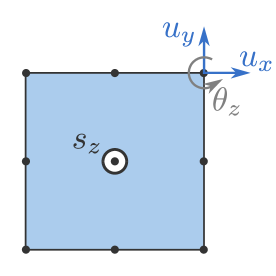
Figure 4: Finite element used for the finite element discretization of the C-CST material model. A second-order Lagrange interpolation is used for displacements and rotations while a constant is used for the skew-symmetric stresses. The nodal degrees of freedom are depicted as black disks while the white disk describes the element skew-symmetric force-stress degree of freedom.

To write the discretized equations, we will use a combined index notation. In this context subscripts will still make reference to scalar components of tensors while capital superscripts will indicate interpolation operations. For instance in the expression

$$u_{i}=_{u}N_{i}^{Q}u^{Q}$$

subscripts $i$ indicate the scalar components of the vector $u$. To facilitate further operations this subscript is also placed in the shape function resulting in terms like ${}_{u}N_{i}^{Q}$ and where the term $u^{Q}$ represents the nodal point displacement associated to the $Q$th nodal point. This nodal vector implicitly considers horizontal and vertical rectangular components. To clarify, the displacement interpolation scheme written here as $u_{i}=_{u}N_{i}^{Q}u^{Q}$ takes the following explicit form for the single nodal point Q:

$$\begin{bmatrix}u_{x}\\ u_{y}\end{bmatrix}=\left[\cdots\begin{array}[]{cc}N^{Q}&0\\ 0&N^{Q}\end{array}\cdots\right]\begin{Bmatrix}\vdots\\ u_{x}^{Q}\\ u_{y}^{Q}\\ \vdots\end{Bmatrix}\,.$$ (47)

With this notation we write for the primary variables $(u_{i},\theta_{i},s_{i})$ the following interpolated versions

$$u_{i}=_{u}N_{i}^{Q}u^{Q},\quad\theta_{i}=_{\theta}N_{i}^{Q}\theta^{Q},\quad s_{i}=_{s}N_{i}^{Q}s^{Q}\,,$$ (48)

and similarly for the secondary kinematic descriptors $e_{ij},\epsilon_{ijk}u_{i,j}$ and $\kappa_{i}$

$$e_{ij}=_{e}B_{ij}^{Q}u^{Q},\quad\epsilon_{ijk}u_{i,j}=_{\nabla}B_{k}^{Q}u^{Q},\quad\kappa_{i}=_{\kappa}B_{i}^{Q}\theta^{Q}\,,$$ (49)

together with the constitutive equations

$$\sigma_{ij}=C_{ijkl}e_{kl}\,,$$ (50)

$$\mu_{i}=D_{ij}\kappa_{j}\,.$$

Substitution of the above relations in (45) gives the discrete version of the first variation of the modified correlated action;

$$\begin{split}&\variation{\hat{\mathcal{A}}}=\delta u^{Q*}\int\limits_{V}(_{e}B_{ij}^{Q})(C_{ijkl})(_{e}B_{kl}^{P})\differential{V}u^{P}-\rho\omega^{2}\delta u^{Q*}\int\limits_{V}(_{u}N_{i}^{Q})(_{u}N_{i}^{P})\differential{V}u^{P}\\ &-\delta u^{Q*}\int\limits_{V}\ {}_{u}N_{i}^{Q}f_{i}\differential{V}-\delta u^{Q*}\int\limits_{S}\ {}_{u}N_{i}^{Q}t_{i}\differential{S}+\delta\theta^{Q*}\int\limits_{V}(_{\kappa}B_{i}^{Q})(D_{ij})(_{\kappa}B_{j}^{P})\differential{V}\theta^{P}\\ &-\delta\theta^{Q*}\int\limits_{S}\ {}_{\theta}N_{i}^{Q}m_{i}\differential{S}+\delta s^{Q*}\int\limits_{V}(_{s}N_{k}^{Q})(_{\nabla}B_{k}^{P})\differential{V}u^{P}+\delta u^{Q*}\int\limits_{V}(_{\nabla}B_{k}^{Q})(_{s}N_{k}^{P})\differential{V}s^{P}\\ &-\delta s^{Q*}\int\limits_{V}2(_{s}N_{k}^{Q})(_{\theta}N_{k}^{P})\differential{V}\theta^{P}-\delta\theta^{Q*}\int\limits_{V}2(_{\theta}N_{k}^{Q})(_{s}N_{k}^{P})\differential{V}s^{P}=0\,.\end{split}$$ (51)

The explicit form of the interpolators defined above is given in the appendix.

5.3 Discrete equilibrium equations

From the arbitrariness in the variations $\delta u^{Q}$ , $\delta\theta^{Q}$ and $\delta s^{Q}$ in (51) it follows that:

$$\begin{split}&\int\limits_{V}(_{e}B_{ij}^{Q})(C_{ijkl})(_{e}B_{kl}^{P})\differential{V}u^{P}-\int\limits_{V}(_{u}N_{i}^{Q})(_{u}N_{i}^{P})\differential{V}u^{P}-\int\limits_{V}\ {}_{u}N_{i}^{Q}f_{i}\differential{V}-\int\limits_{S}\ {}_{u}N_{i}^{Q}t_{i}\differential{S}=0\,,\\ &\int\limits_{V}(_{\kappa}B_{i}^{Q})(D_{ij})(_{\kappa}B_{j}^{P})\differential{V}\theta^{P}-\int\limits_{S}\ {}_{\theta}N_{i}^{Q}m_{i}\differential{S}-\int\limits_{V}2(_{\theta}N_{k}^{Q})(_{s}N_{k}^{P})\differential{V}s^{P}=0\,,\\ &\int\limits_{V}(_{s}N_{k}^{Q})(_{\nabla}B_{k}^{P})\differential{V}u^{P}-\int\limits_{V}2(_{s}N_{k}^{Q})(_{\theta}N_{k}^{P})\differential{V}\theta^{P}=0\,,\end{split}$$

which can be written in the standard finite element form for dynamic equilibrium

$$\begin{bmatrix}K_{uu}^{QP}&0&K_{us}^{QP}\\ 0&K_{\theta\theta}^{QP}&-K_{\theta s}^{QP}\\ K_{su}^{QP}&-K_{s\theta}^{QP}&0\end{bmatrix}\begin{Bmatrix}u^{P}\\ \theta^{P}\\ s^{P}\end{Bmatrix}=\omega^{2}\begin{bmatrix}M_{uu}^{QP}&0&0\\ 0&0&0\\ 0&0&0\end{bmatrix}\begin{Bmatrix}u^{P}\\ \theta^{P}\\ s^{P}\end{Bmatrix}+\begin{Bmatrix}F_{u}^{Q}\\ m_{\theta}^{Q}\,\\ 0\end{Bmatrix}$$ (52)

where the individual terms are defined as

$$K_{uu}^{QP} =\int\limits_{V}(_{e}B_{ij}^{Q})(C_{ijkl})(_{e}B_{kl}^{P})\differential{V}\,, M_{uu}^{QP} =\rho\omega^{2}\int\limits_{V}(_{u}N_{i}^{Q})(_{u}N_{i}^{p})\differential{V}\,,$$

$$K_{us}^{QP} =\int\limits_{V}(_{\nabla}B_{k}^{Q})(_{s}N_{k}^{P})\differential{V}\,, F_{u}^{Q} =\int\limits_{V}\ {}_{u}N_{i}^{Q}f_{i}\differential{V}+\int\limits_{S}\ {}_{u}N_{i}^{Q}t_{i}\differential{S}\,,$$

$$K_{\theta\theta}^{QP} =\int\limits_{V}(_{\kappa}B_{i}^{Q})(D_{ij})(_{\kappa}B_{j}^{P})\differential{V}\,, K_{\theta s}^{QP} =\int\limits_{V}2(_{\theta}N_{k}^{Q})(_{s}N_{k}^{P})\differential{V}\,,$$

$$m_{\theta}^{Q} =\int\limits_{S}\ {}_{\theta}N_{i}^{Q}m_{i}\differential{S}\,, K_{su}^{QP} =\int\limits_{V}(_{s}N_{k}^{Q})(_{\nabla}B_{k}^{P})\differential{V}\,,$$

$$K_{s\theta}^{QP} =\int\limits_{V}2(_{s}N_{k}^{Q})(_{\theta}N_{k}^{P})\differential{V}\,.$$

Equation 52 can be rewritten in the following set of equilibrium equations in terms of nodal forces and couples

$$f_{(\sigma)}^{Q}+f_{s}^{Q}-f_{I}^{Q}-T^{Q} =0\,,$$ (53)

$$m_{\mu}^{Q}+m_{s}^{Q}-q^{Q} =0\,,$$

$$s(\theta-\hat{\theta})=0\,,$$

where the subindex $(\sigma)$ refers to the symmetric part of the stress tensor, and $I$ to inertial forces. Notice that we do not have an inertial term for the second equation as is the case for the micropolar model (Guarín-Zapata et al., 2020). We also have a third equation reflecting the kinematic restriction, between the rotation $\theta$ and the introduced degree of freedom $\hat{\theta}$, imposed via the Lagrange-multiplier term $s$ in each element.

When using a Lagrange multiplier formulation as in (45) the equations are still self-adjoint, as can be seen in the structure of (52). Nevertheless, the stiffness matrix is indefinite and the solution of the problem represents a saddle-point instead of a minimum (Arnold, 1990; Darrall et al., 2014).

5.4 Eigenvalue problem

In finding the dispersion relations, we are interested in the free wave motion in the media. This leads to the following eigenvalue problem

$$[K]\{U\}=\omega^{2}[M]\{U\}$$ (54)

with

$$[K]=\begin{bmatrix}K_{uu}^{QP}&0&K_{us}^{QP}\\ 0&K_{\theta\theta}^{QP}&-K_{\theta s}^{QP}\\ K_{su}^{QP}&-K_{s\theta}^{QP}&0\end{bmatrix},\,[M]=\begin{bmatrix}M_{uu}^{QP}&0&0\\ 0&0&0\\ 0&0&0\end{bmatrix},\,\{U\}=\begin{Bmatrix}u^{P}\\ \theta^{P}\\ s^{P}\end{Bmatrix}\,.$$

In (54) Bloch-periodic boundary conditions are yet to be imposed. This can be done in two ways (Valencia et al., 2019): (i) modifying the connectivity of the elements; and (ii) assembling the matrices without considering boundary conditions and impose the Bloch-periodicity through row/column operations. In this work, we follow the second approach as it requires the stiffness and mass matrices to be assembled once and the transformation matrices are computed for every wavenumber in the first Brillouin zone. This process results in the following eigenvalue problem

$$[K_{R}(\mathbf{k})]\{U\}=\omega^{2}[M_{R}(\mathbf{k})]\{U\}$$ (55)

with

$$[K_{R}(\mathbf{k})]=[T(\mathbf{k})^{H}KT(\mathbf{k})]\,,\quad[M_{R}(\mathbf{k})]=[T(\mathbf{k})^{H}MT(\mathbf{k})]\,,$$

where $[T(\mathbf{k})]$ represents the transformation matrix for a given $\mathbf{k}$, and the $[T^{H}]$ refers to the Hermitian transpose of $[T]$. For an explicit form for the matrices $[T]$ refer to Hussein et al. (2014) or Guarín-Zapata (2012).

We conducted the implementation on top of the in-house finite element code SolidsPy (Gómez and Guarín-Zapata, 2018) and used SciPy to solve the eigenvalue problem (Virtanen et al., 2020). To take advantage of the sparsity of the matrices the problem should be written as matrix-vector multiplications, such as

$$\{x\}=[T]\{U\}\,,$$

$$\{y\}=[K]\{x\}\,,$$

$$\{z\}=[T^{H}]\{y\}\,,$$

with $\{z\}$ representing the image of the linear operator $[K_{R}]$ over $\{U\}$. The same procedure can be applied for the right-hand side of (55).

The Lagrange-multiplier approach represents a saddle-point instead of a minimization problem (Arnold, 1990). This can be seen in the structure of the stiffness matrix obtained in equation (54). Furthermore the mass matrix is not positive definite anymore. This structure for the eigenvalue problem requires the use of a specific solver such as the LOBPCG method (Knyazev, 2001) instead of the classical Arnoldi method (Lehoucq et al., 1998).

6 Results: Dispersion relations for C-CST cellular materials

In this section we conduct a series of dispersion analyses intended to show the effectiveness of our mixed finite element implementation of the C-CST material model in predicting the correct wave propagation properties of the material. All the dispersion graphs use the dimensionless frequency

$$\Omega=\frac{2d\omega}{c_{2}}\,,$$ (56)

for the vertical axis, where $2d$ is the dimension of the unit cell and $c_{2}^{2}=\mu/\rho$ is the speed of the shear wave for a classical elastic material. The Poisson ratio for all the simulations is $\nu=1/4$.

As a first instance we find the response of a homogeneous periodic material which has also a closed form solution. We will then continue to study a second prototypical example corresponding to a homogeneous material with a circular pore. These two problems exhibit two different levels of dispersive behavior. In the homogeneous material cell, dispersion is due to the kinematic enrichment of the model associated to the length scale parameter, while in the porous material model additional dispersion arises due to the explicit microstructural feature.

6.1 Homogeneous material

As a test of accuracy and effectiveness of our implementation we consider the case of a homogeneous material cell with the same mechanical properties of the material reported previously and with closed form dispersion relations from (16) and (17). In this model microstructural effects are introduced through the material length parameter $\ell$. Recall that $\ell^{2}$ is defined by the ratio $\frac{\eta}{\mu}$ where $\eta$ is the curvature-couple-stress module while $\mu$ is the shear modulus from Cauchy elasticity. The results in terms of the resulting band structure are shown in fig. 5, where we used a $16\times 16$ mesh and $\ell^{2}/d^{2}=3/8$. For a conceptual description of the reciprocal space and a guide on how to interpret the results in a Bloch analysis the reader is referred to Valencia (2019). Note that this set of results is directly comparable with the curves from the closed form solutions from fig. 2. Since the material is isotropic there are no directional effects and, as discussed previously, the only difference between this model and the result from classical elasticity is the dispersive behavior of the shear wave. In contrast with the micropolar model (Guarín-Zapata et al., 2020), the present C-CST model does not exhibit additional rotational waves.

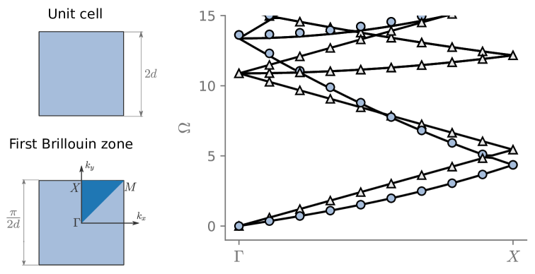
Figure 5: Dispersion relations for a homogeneous material model. Solid lines represent FEM results while markers correspond to the analytic solution. Triangular and filled-dots describe the P and SV wave modes, respectively.

Figure 6 shows the results for the same material cell but now we have considered 4 different values of the length scale parameter corresponding to $\ell/d\in[0.01,0.1,1,10]$. The mesh in this case is $16\times 16$. Notice that, as expected, the increasing value of this parameter only affects the dispersive response of the shear waves while the P-waves retain their classical non-dispersive behavior. As seen in (17) the dispersion increases for higher values of $\ell$ due to the factor $\sqrt{1+k^{2}\ell^{2}}$ in the dispersion relation. This behavior is closely followed by the numerical results presented in fig. 6.

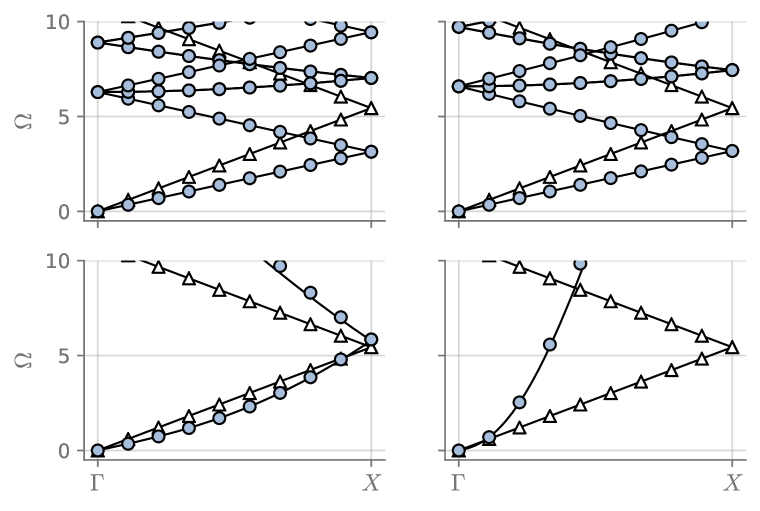
Figure 6: Dispersion relations for a homogeneous material model with varying length scales, $\ell/d\in[0.01,0.1,1,10]$. Solid lines represent FEM results while markers correspond to analytic solutions. As expected, for increasing $\ell/d$ the S-wave presents more dispersion due to the factor $\sqrt{1+k^{2}\ell^{2}}$, as presented in (17).

As an additional verification, we also tested the convergence in the calculation of the dispersion relations after considering the first 8 modes for a sequence of meshes of $1\times 1$, $2\times 2$, $4\times 4$, and $8\times 8$ elements for $\ell^{2}/d^{2}=3/8$. The error in the eigenvalue computation was measured according to

$$e=\frac{\|{\bf\it\omega}_{\text{ref}}-{\bf\it\omega}_{h}\|_{2}}{\|{\bf\it\omega}_{\text{ref}}\|_{2}}\,,$$

where ${\bf\it\omega}_{h}$ is the set of eigenvalues (dispersion relation) for a mesh of characteristic element size $h$ and ${\bf\it\omega}_{\text{ref}}$ is the solution corresponding to the finer $16\times 16$ elements mesh, which has been taken as reference. The results for this sequence, together with the variation in the error parameter, are displayed in fig. 7. The estimated convergence rate for the eigenvalues is 2.32. We see that when we refine the mesh it can reproduce the dispersion curves better for higher frequencies. There are still some differences between the $8\times 8$ and $16\times 16$ meshes around the dimensionless frequency of 15 but these differences will disappear with further refinement. Nevertheless, opposed to what happens in classical continua we would need more points per wavelength every time that we want to increase the maximum frequency. This is due to the inherent dispersive behavior of S-waves as can be seen in equation (17). Thus, we would expect to need more than 10 points per wavelength, customary for finite element methods, or 5, customary for spectral element methods (Komatitsch and Tromp, 1999; Ainsworth and Wajid, 2009; Guarín-Zapata and Gomez, 2015). Again, we should emphasize the dispersive nature of the SV-waves, while the P-waves remain non-dispersive.

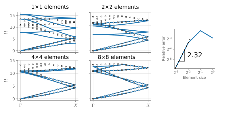
Figure 7: Convergence of the first 8 modes in the dispersion relations at $\ell^{2}/d^{2}=3/8$ for a sequence of meshes with: $1\times 1$, $2\times 2$, $4\times 4$, and $8\times 8$ elements — presented as solid blue lines in the background. The results are compared with a mesh that has $16\times 16$ elements — presented as dots in the foreground. The estimated convergence rate for the eigenvalues in the 2-norm is 2.32.

6.2 Dispersion in cellular material with a circular pore

Now, we consider a C-CST composite material cell configured by a circular pore embedded in a homogeneous matrix. The presence of the pore provides the model with a second length-scale due to the microstructure, in addition to the one introduced by the material length-scale parameter $\ell$. For illustration, we assume a pore diameter $a$ that is half the cell length (i.e., $a=d$). Thi is equivalent to a porosity of $\pi/16$ or approximately 0.196, which is kept fixed as we modify the size of the unit cell to control $\ell/a$.

The resulting dispersion curves for this cellular material with four different length scale ratios are shown in fig. 8 with $\ell/a=[0.01,0.1,1,10]$. In contrast to the results from the fully homogeneous material cell, the presence of the circular pore introduces scattering effects inside each cell and the composite shows much more complicated elastodynamic behavior. Most importantly, however, the dispersion curves become more regular with increased $\ell/a$ and partial bandgaps open up along the $\Gamma M$ and $X\Gamma$ directions, especially for $\ell/a=1$ and $\ell/a=10$. This type of band structure is not observed for classical elastodynamic cells with a similar geometric periodicity, which would exhibit behavior close to that obtained here with $\ell/a=0.01$. In fact, as $\ell/a\rightarrow 0$, C-CST theory recovers the classical result.

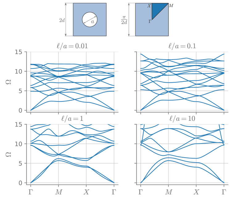
Figure 8: Dispersion for a cellular material with circular pores for varying length scales, $\ell/a=[0.01,0.1,1,10]$.

Furthermore, it is important to note that this interesting band structure is obtained with a consistent continuum mechanics formulation, which requires only a single additional material parameter, $\ell$, beyond those needed in the classical elastic case. When this intrinsic length scale is on the order of the hole diameter, the dispersive SV wave has a fundamental group velocity for the cell with dimension $2d$ approximately equal to the group (and phase) velocity of the non-dispersive P wave, which allows the SV and P branches to follow a similar path, causing band gaps to open. This behavior, which is not seen in classical elastodynamics, occurs in the regions near to where the two branches intersect in fig. 2. Consequently, under C-CST, these band gaps will originate whenever the size of the cellular structure is tuned to the material length scale, a potentially significant phenomenon that has not been recognized previously. With further tuning of the porosity level and cell size, it may be possible to achieve even a complete bandgap at relatively low non-dimensional frequency $\Omega$.

7 Conclusions

The present work incorporates several innovative aspects. First of all, we have developed a novel frequency domain correlated action principle for the consistent couple stress theory (C-CST) of Hadjesfandiari and Dargush (2011) and used that to extend the Lagrange multiplier finite element algorithm of Darrall et al. (2014) to study periodic cellular materials through Floquet-Bloch theory from solid state physics. Particularly, we have addressed the imposition of extended Bloch boundary conditions for this material model where in addition to force tractions and displacements there are also couple tractions and rotations. Secondly, we also discussed numerical aspects related to the solution of the wavenumber dependent generalized eigenvalue problem resulting from the imposition of the Bloch periodic boundary conditions, overcoming complications arising from the inclusion of Lagrange multipliers and a non-positive definite mass matrix. The implementation was shown to give accurate results for homogeneous and porous unit cells and for varying couple stress material length-scale parameters.

The analysis of the first cell was used mainly to test the correctness of our implementation as this material has a closed-form dispersion relation. The algorithm was shown to correctly capture the non-dispersive P-wave as well as the dispersive SV-wave. This analysis was complemented by a convergence analysis with four different meshes of increasing refinement for the material cell. The observed convergence rate shows that the Lagrange multiplier algorithm is effective in maintaining continuity by imposing the newly introduced kinematic constraint implicit in the mean curvature tensor definition. As the final contribution, we have discovered the interesting bandgap structure of a material cell with a circular pore embedded in a homogeneous matrix, which reveals the appearance of bandgaps introduced by the kinematic features of C-CST and the dispersive behavior of the SV-waves defined in terms of the microstructural length scale parameter.

From a general perspective, C-CST is a true size-dependent continuum theory, which is intended here for periodic elastic material cells at scales for which a continuum representation is appropriate. From the results shown in the paper, C-CST becomes important when the size of the cell in on the order of the intrinsic length scale parameter or smaller. For larger cells, the classical theory can be used instead. On the other hand, micropolar theory disconnects the rotational field from the displacements, which can lead to approximations that may or may not be physical.

Appendix A Explicit form of the finite element interpolators in the C-CST solid

In the case of isotropic materials under plane strain idealizations, we have the following equations

$$\left(\lambda+2\mu\right)\left(\frac{d^{2}u_{x}}{dx^{2}}+\frac{d^{2}u_{y}}{dydx}\right)-\mu\left(\frac{d^{2}u_{y}}{dydx}-\frac{d^{2}u_{x}}{dy^{2}}\right)-\eta\left(\frac{d^{4}u_{x}}{dy^{4}}+\frac{d^{4}u_{x}}{dy^{2}dx^{2}}-\frac{d^{4}u_{y}}{dy^{3}dx}-\frac{d^{4}u_{y}}{dydx^{3}}\right)=-\rho\omega^{2}u_{x}$$

$$\left(\lambda+2\mu\right)\left(\frac{d^{2}u_{y}}{dy^{2}}+\frac{d^{2}u_{x}}{dydx}\right)-\mu\left(\frac{d^{2}u_{x}}{dydx}-\frac{d^{2}u_{y}}{dx^{2}}\right)-\eta\left(\frac{d^{4}u_{y}}{dx^{4}}-\frac{d^{4}u_{x}}{dy^{3}dx}-\frac{d^{4}u_{x}}{dydx^{3}}+\frac{d^{4}u_{y}}{dy^{2}dx^{2}}\right)=-\rho\omega^{2}u_{y}$$

We have the following explicit forms for the interpolation matrices in two dimensions (Bathe (1995)):

$${}_{u}\mathbf{N}^{Q} =_{\theta}\mathbf{N}^{Q}=_{s}\mathbf{N}^{Q}=\begin{bmatrix}\cdots&N^{Q}&0&\cdots\\ \cdots&0&N^{Q}&\cdots\end{bmatrix}\,, {}_{e}\mathbf{B}=\begin{bmatrix}\cdots&\frac{\partial N^{Q}}{\partial x}&0&\cdots\\ \cdots&0&\frac{\partial N^{Q}}{\partial x}&\cdots\\ \cdots&\frac{\partial N^{Q}}{\partial y}&\frac{\partial N^{Q}}{\partial x}&\cdots\end{bmatrix}\,,$$

$${}_{\kappa}\mathbf{B} =\begin{bmatrix}\cdots&-\frac{\partial N^{Q}}{\partial y}&\cdots\\ \cdots&\frac{\partial N^{Q}}{\partial x}&\cdots\end{bmatrix}\,, \mathbf{{}_{\nabla}B}=\begin{bmatrix}\cdots&-\frac{\partial N^{Q}}{\partial y}&\frac{\partial N^{Q}}{\partial x}&\cdots\end{bmatrix}\,.$$

an the following constitutive tensors in Voigt notation

$$\mathbf{C}=\frac{E(1-\nu)}{(1+\nu)(1-2\nu)}\begin{bmatrix}1&\frac{\nu}{1-\nu}&0\\ \frac{\nu}{1-\nu}&1&0\\ 0&0&\frac{1-2\nu}{2(1-\nu)}\end{bmatrix}\,,\quad \mathbf{D}=4\eta\begin{bmatrix}1&0\\ 0&1\end{bmatrix}\,.$$

References

- Ainsworth and Wajid (2009) Mark Ainsworth and Hafiz Abdul Wajid. Dispersive and dissipative behavior of the spectral element method. SIAM Journal on Numerical Analysis, 47(5):3910–3937, 2009.
- Arfken et al. (2005) George B. Arfken, Hans J. Weber, and Frank Harris. Mathematical Methods for Physicists. Academic Press, 6 edition, 2005.
- Arnold (1990) Douglas N. Arnold. Mixed finite element methods for elliptic problems. Computer Methods in Applied Mechanics and Engineering, 82(1):281–300, September 1990. ISSN 0045-7825. doi: 10.1016/0045-7825(90)90168-L. URL http://www.sciencedirect.com/science/article/pii/004578259090168L.
- Banerjee (2011) Biswajit Banerjee. An introduction to metamaterials and waves in composites. Crc Press, 2011.
- Bathe (1995) Klaus-Jurgen Bathe. Finite Element Procedures. Prentice Hall, 2 edition, 6 1995.
- Bloch (1929) Felix Bloch. Über die quantenmechanik der elektronen in kristallgittern. Zeitschrift für physik, 52(7-8):555–600, 1929.
- Brillouin (1953) Leon Brillouin. Wave propagation in periodic structures: Electric filters and crystal lattices. Dover Publications, 1 edition, 1953.
- Cao et al. (2004) Yongjun Cao, Zhilin Hou, and Youyan Liu. Convergence problem of plane-wave expansion method for phononic crystals. Physics Letters A, 327(2-3):247–253, 2004.
- Chakravarty et al. (2017) Sourish Chakravarty, Ali R. Hadjesfandiari, and Gary F. Dargush. A penalty-based finite element framework for couple stress elasticity. Finite Elements in Analysis and Design, 130:65–79, 2017.
- Chin et al. (2021) Eric B Chin, Amir Ashkan Mokhtari, Ankit Srivastava, and N Sukumar. Spectral extended finite element method for band structure calculations in phononic crystals. Journal of Computational Physics, 427:110066, 2021.
- Cosserat and Cosserat (1909) E. Cosserat and F. Cosserat. Théorie des Corps Déformables. A Hermann et Fils, 1909.
- Dal Poggetto and Serpa (2020) VF Dal Poggetto and Alberto Luiz Serpa. Elastic wave band gaps in a three-dimensional periodic metamaterial using the plane wave expansion method. International Journal of Mechanical Sciences, 184:105841, 2020.
- Darrall et al. (2014) Bradley T. Darrall, Gary F. Dargush, and Ali R. Hadjesfandiari. Finite element lagrange multiplier formulation for size-dependent skew-symmetric couple-stress planar elasticity. Acta Mechanica, 225(1):195–212, 2014.
- Deng and Dargush (2016) Guoqiang Deng and Gary F. Dargush. Mixed Lagrangian formulation for size-dependent couple stress elastodynamic response. Acta Mechanica, 227(12):3451–3473, 2016.
- Deng and Dargush (2017) Guoqiang Deng and Gary F. Dargush. Mixed lagrangian formulation for size-dependent couple stress elastodynamic and natural frequency analyses. International Journal for Numerical Methods in Engineering, 109(6):809–836, 2017.
- Eringen and Suhubi (1964) A Cemal Eringen and ES Suhubi. Nonlinear theory of simple micro-elastic solids—i. International Journal of Engineering Science, 2(2):189–203, 1964.
- Eringen (1966) A.C Eringen. Linear theory of micropolar elasticity. Journal of Mathematics and Mechanics, 15:909–923, 1966.
- Floquet (1883) Gaston Floquet. Sur les équations différentielles linéaires à coefficients périodiques. In Annales scientifiques de l’École normale supérieure, volume 12, pages 47–88, 1883.
- Guarín-Zapata and Gomez (2015) Nicolás Guarín-Zapata and Juan Gomez. Evaluation of the spectral finite element method with the theory of phononic crystals. Journal of Computational Acoustics, 23(02):1550004, 2015.
- Guarín-Zapata et al. (2020) Nicolás Guarín-Zapata, Juan Gomez, Camilo Valencia, Gary F. Dargush, and Ali Reza Hadjesfandiari. Finite element modeling of micropolar-based phononic crystals. Wave Motion, 92:102406, 2020.
- Guarín-Zapata (2012) Nicolás Guarín-Zapata. Simulación Numérica de Problemas de Propagación de Ondas: Dominios Infinitos y Semi-infinitos. Master’s thesis, Universidad EAFIT, 2012.
- Gómez and Guarín-Zapata (2018) Juan Gómez and Nicolás Guarín-Zapata. Solidspy: 2d-finite element analysis with python, 2018. URL https://github.com/AppliedMechanics-EAFIT/SolidsPy.
- Hadjesfandiari and Dargush (2011) Ali R Hadjesfandiari and Gary F Dargush. Couple stress theory for solids. International Journal of Solids and Structures, 48(18):2496–2510, 2011.
- Hussein et al. (2014) Mahmoud I Hussein, Michael J Leamy, and Massimo Ruzzene. Dynamics of phononic materials and structures: Historical origins, recent progress, and future outlook. Applied Mechanics Reviews, 66(4):040802, 2014.
- Isakari et al. (2016) Hiroshi Isakari, Toru Takahashi, and Toshiro Matsumoto. Periodic band structure calculation by the sakurai–sugiura method with a fast direct solver for the boundary element method with the fast multipole representation. Engineering Analysis with Boundary Elements, 68:42–53, 2016.
- Johnson (2010) Steven G. Johnson. Notes on the algebraic structure of wave equations. Technical report, Massachusetts Institute of Technology, 2010. URL https://pdfs.semanticscholar.org/83a2/7bf232399defbaf1ff63e402412a5c6cbb2c.pdf.
- Kittel (1996) Charles Kittel. Introduction to Solid State Physics. Wiley, 7 edition, 1996.
- Knyazev (2001) Andrew V. Knyazev. Toward the optimal preconditioned eigensolver: Locally optimal block preconditioned conjugate gradient method. SIAM journal on scientific computing, 23(2):517–541, 2001.
- Koiter (1964) W.T Koiter. Couple stresses in the theory of elasticity. Proc.K.Ned.Akad.Wet(B), 67:17–44, 1964.
- Komatitsch and Tromp (1999) Dimitri Komatitsch and Jeroen Tromp. Introduction to the spectral element method for three-dimensional seismic wave propagation. Geophysical journal international, 139(3):806–822, 1999.
- Kreyszig (1978) Erwin Kreyszig. Introductory functional analysis with applications, volume 1. wiley New York, 1978.
- Langlet et al. (1995) Philippe Langlet, Anne-Christine Hladky-Hennion, and Jean-Noël Decarpigny. Analysis of the propagation of plane acoustic waves in passive periodic materials using the finite element method. Journal of the Acoustical Society of America, 98(5):2792–2800, 11 1995.
- Lehoucq et al. (1998) Richard B. Lehoucq, Danny C. Sorensen, and Chao Yang. ARPACK users’ guide: solution of large-scale eigenvalue problems with implicitly restarted Arnoldi methods, volume 6. Siam, 1998.
- Li et al. (2013a) Feng-Lian Li, Yue-Sheng Wang, Chuanzeng Zhang, and Gui-Lan Yu. Bandgap calculations of two-dimensional solid–fluid phononic crystals with the boundary element method. Wave Motion, 50(3):525–541, 2013a.
- Li et al. (2013b) Feng-Lian Li, Yue-Sheng Wang, Chuanzeng Zhang, and Gui-Lan Yu. Boundary element method for band gap calculations of two-dimensional solid phononic crystals. Engineering Analysis with Boundary Elements, 37(2):225–235, 2013b.
- Mazzotti et al. (2019) Matteo Mazzotti, Ivan Bartoli, and Marco Miniaci. Modeling bloch waves in prestressed phononic crystal plates. Frontiers in Materials, 6:74, 2019.
- Mindlin (1964) R. Mindlin. Micro-structure in linear elasticity. Archives of Rational Mechanics and Analysis, 16:51–78, 1964.
- Mindlin and Tiersten (1962) R. Mindlin and H. Tiersten. Effects of couple-stresses in linear elasticity. Archives of Rational Mechanics and Analysis, 11:415–448, 1962.
- Nowacki (1986) Witold Nowacki. Theory of asymmetric elasticity. Pergamon Press, Headington Hill Hall, Oxford OX 3 0 BW, UK, 1986., 1986.
- Pedgaonkar et al. (2021) Akhilesh Pedgaonkar, Bradley T Darrall, and Gary F Dargush. Mixed displacement and couple stress finite element method for anisotropic centrosymmetric materials. European Journal of Mechanics-A/Solids, 85:104074, 2021.
- Reddy (1986) Junuthula Narasimha Reddy. Applied functional analysis and variational methods in engineering. Mcgraw-Hill College, 1986.
- Su et al. (2010) Xiao-Xing Su, Jian-Bao Li, and Yue-Sheng Wang. A postprocessing method based on high-resolution spectral estimation for fdtd calculation of phononic band structures. Physica B: Condensed Matter, 405(10):2444–2449, 2010.
- Tanaka et al. (2000) Yukihiro Tanaka, Yoshinobu Tomoyasu, and Shin-ichiro Tamura. Band structure of acoustic waves in phononic lattices: Two-dimensional composites with large acoustic mismatch. Physical Review B, 62(11):7387, 2000.
- Toupin (1962) R. A. Toupin. Elastic materials with couple-stresses. Archives of Rational Mechanics and Analysis, 11:385–414, 1962.
- Valencia (2019) Camilo Valencia. Wave propagation in 2D elastic periodic materials: theoretical and computational analysis. PhD thesis, Universidad EAFIT, 2019.
- Valencia et al. (2019) Camilo Valencia, Juan Gómez, and Nicolás Guarín-Zapata. A general purpose element-based approach to compute dispersion relations in periodic materials with existing finite element codes. Journal of Theoretical and Computational Acoustics, 2019. doi: 10.1142/S2591728519500051.
- Virtanen et al. (2020) Pauli Virtanen, Ralf Gommers, Travis E. Oliphant, Matt Haberland, Tyler Reddy, David Cournapeau, Evgeni Burovski, Pearu Peterson, Warren Weckesser, Jonathan Bright, et al. SciPy 1.0: fundamental algorithms for scientific computing in Python. Nature methods, 17(3):261–272, 2020.
- Voigt (1910) W. Voigt. Lehrbuch der Kristalphysik. Teubner, B, 1910.
- Xie et al. (2017) Longxiang Xie, Baizhan Xia, Jian Liu, Guoliang Huang, and Jirong Lei. An improved fast plane wave expansion method for topology optimization of phononic crystals. International Journal of Mechanical Sciences, 120:171–181, 2017.
- Zhang et al. (2018) Peng Zhang, Peijun Wei, and Yueqiu Li. The elastic wave propagation through the finite and infinite periodic laminated structure of micropolar elasticity. Composite Structures, 2018.