ModelDiff: Testing-Based DNN Similarity Comparison for Model Reuse Detection

Abstract.

The knowledge of a deep learning model may be transferred to a student model, leading to intellectual property infringement or vulnerability propagation. Detecting such knowledge reuse is nontrivial because the suspect models may not be white-box accessible and/or may serve different tasks. In this paper, we propose ModelDiff, a testing-based approach to deep learning model similarity comparison. Instead of directly comparing the weights, activations, or outputs of two models, we compare their behavioral patterns on the same set of test inputs. Specifically, the behavioral pattern of a model is represented as a decision distance vector (DDV), in which each element is the distance between the model’s reactions to a pair of inputs. The knowledge similarity between two models is measured with the cosine similarity between their DDVs. To evaluate ModelDiff, we created a benchmark that contains 144 pairs of models that cover most popular model reuse methods, including transfer learning, model compression, and model stealing. Our method achieved 91.7% correctness on the benchmark, which demonstrates the effectiveness of using ModelDiff for model reuse detection. A study on mobile deep learning apps has shown the feasibility of ModelDiff on real-world models.

1. Introduction

Deep learning models (i.e. deep neural networks, or DNNs for short) are increasingly deployed into various applications for a wide range of tasks. Due to the difficulty of building accurate and efficient models from scratch, various model reuse techniques have been proposed to help developers build models based on existing models. The knowledge of an existing model can be transferred to new models that are tailored for different application scenarios and/or resource constraints. For example, transfer learning (Pan and Yang, 2009) can be used to adapt the existing models trained for one task to solve other similar tasks. Model compression techniques (Han et al., 2015a) can convert a large model to a smaller one to deploy in resource-constrained environments while reserving reasonable accuracy. Due to the great convenience and remarkable performance, these techniques are increasingly used by deep learning developers today.

However, the ability of knowledge transfer also leads to concerns about intellectual property (IP) and vulnerability propagation. First, a deep learning model is usually an important property for a company given the difficulty of training it (Coleman et al., 2017). Reusing a model without authorization or license compliance would violate the IP right. Second, some pretrained models may have security defects (such as adversarial vulnerability (Szegedy et al., 2013), backdoors (Liu et al., 2018b; Li et al., 2021), etc.), and the models based on them may inherit the defects (Davchev et al., 2019; Yao et al., 2019). Similar problems exist in traditional programs where the code may be plagiarized or reused, and software similarity analysis (Rattan et al., 2013; Ragkhitwetsagul et al., 2018; Guo et al., 2018) is one of the most popular techniques to address such problems.

Analyzing the similarity between deep learning models involves three key challenges. First, the models under comparison, especially the suspect models built upon pretrained models are usually not white-box accessible, since many of them are deployed on a server and provided to customers through inference APIs. Second, even if the models are available for structure or weight comparison, the structural similarity does not necessarily mean knowledge similarity: Two unrelated DNNs may have identical or similar structures, since they may use the same public state-of-the-art model architecture (e.g. ResNet, MobileNet, etc.). Meanwhile, two closely related DNNs may have significantly different structures and weights, for example when one is generated from another through knowledge distillation. Third, the models that contain common knowledge may appear quite different since they may use the knowledge for different tasks (e.g. an object detection model built upon an image classification model through transfer learning).

In this paper, we propose ModelDiff, a testing-based approach to DNN model similarity comparison. Instead of directly comparing the graph structures and weights that may be unavailable or incomparable, we compare the decision patterns of the models based on how they respond to the same set of test inputs. Measuring knowledge similarity from the testing perspective directly solves the first two challenges stated above since it only requires black-box access to the suspect models and no comparison of the internal structures is needed. However, due to the third challenge (the models may belong to different tasks), the test outputs of different models are not directly comparable. Thus we introduce a new data structure, named decision distance vector (DDV), to represent the decision logic of a model on the test inputs. Each value in a DDV is the distance between the outputs of the model produced by two inputs. The insight behind DDVs is that two models would group the test inputs with a similar pattern if their decision boundaries are similar. Since the size of a DDV is only related to the number of inputs used to test the model, the DDVs generated with the same set of samples are comparable across different models. As a result, the knowledge similarity between DNNs can be measured based on the distance between their DDVs. An illustration of the idea is shown in Figure 1.

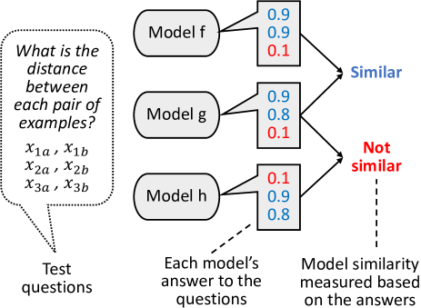
Figure 1. An illustration of the idea of ModelDiff to measure knowledge similarity between DNN models.

To detect model reuse, a key problem of ModelDiff is how to generate the test inputs that can represent the unique decision pattern of a model that is exclusively shared by the models built upon it. Using normal samples as test inputs is ineffective because the normal inputs are usually processed by the common-sense knowledge that is shared across unrelated models. For example, feeding a normal cat image to different image classifiers would lead to similar outputs, although the classifiers might be trained with completely different datasets and algorithms.

Inspired by prior work on adversarial attack transferability (Demontis et al., 2019; Huang et al., 2019; Davchev et al., 2019), we use both normal and adversarial inputs to construct the test inputs. The insight is that the normal inputs and adversarial inputs are processed by the normal and imperfect knowledge of a model respectively, while the decision boundary of the model can be characterized by the combination of normal and imperfect knowledge. Specifically, given two models under comparison, one of them is selected as the target model and another is the suspect model. The test inputs in ModelDiff are generated based on a set of normal samples (named seed inputs) that lie in the input distribution of the target model. We find an adversarial input for each seed input by maximizing the divergence between the model’s predictions on adversarial and normal inputs and the diversity of the model predictions produced by the test inputs. Each adversarial input and the corresponding normal input are paired to compute DDVs that depict the decision boundary precisely and completely. Such DDVs can capture the similarity between teacher and student model because the decision boundaries are transferred during model reuse.

To evaluate our approach, we created a benchmark named ModelReuse. ModelReuse contains 114 models generated from large pretrained models using various model reuse techniques. Based on these models, we obtained 144 pairs of models that have reused knowledge, including 84 direct reuses (one is generated from another using a single model reuse method) and 60 combined reuses (one is generated from another using a combination of transfer learning and model compression). We evaluated ModelDiff by examining whether it can be applied to detect these reuses (feasibility) and whether it can correctly compute higher similarity scores for the model pairs with reused knowledge (correctness).

ModelDiff could support meaningful comparison for all model pairs in ModelReuse benchmark and achieved an overall correctness of 91.7%, which outperformed both the white-box and black-box baseline methods that we created based on weight, feature map, and fingerprint comparison.

To better understand the knowledge similarity measured with ModelDiff, we further analyzed the relation between the similarity score and the model accuracy. The result shows that the similarity score computed by ModelDiff is in general proportional to model accuracy, i.e. a higher similarity between two models typically means more useful knowledge of one model is utilized by another, leading to higher test accuracy.

Finally, to examine whether ModelDiff can be used to measure model similarity in the wild, we collected 35 TFLite models from 20,000 real-world Android apps in Google Play and compared them with a popular pretrained model using ModelDiff. Our method was able to handle these real-world black-box models, and the knowledge similarities measured for these models were consistent with our manual inspection based on the model file names.

This paper makes the following key contributions:

1. To the best of our knowledge, this is the first work that systematically discusses the problem of DNN model reuse detection, where the student model and teacher model may be heterogeneous, black-box, and serving different tasks.

2. We introduce a benchmark named ModelReuse for model reuse detection, which contains 144 models generated with popular model reuse techniques with varying configurations.

3. We propose ModelDiff, a testing-based method for model similarity comparison. Our method achieved 91.7% correctness on ModelReuse benchmark. Both the benchmark and the tool will be released to the community.

2. Background: DNN Model Reuse

Building an efficient and accurate DNN model from scratch is a data-intensive and time-consuming task, thus it is common for developers to build DNNs based on existing pretrained DNNs. This section will introduce transfer learning and model compression, two widely-used techniques for adapting a DNN model to different tasks and different resource constraints, and model stealing, a malicious way to transfer the knowledge of a model. We call the models being reused as teacher models and the models that inherent knowledge from teacher models as student models.

2.1. Transfer Learning

Transfer learning aims to transfer the knowledge of a pretrained teacher model to a student model used for a different but related problem. For example, an image classifier that predicts the type of animals in the input images can transfer knowledge to a more specific classifier that predicts the breeds of cats, or to an object detector that predicts the location of each animal in the image. The reason why transfer learning is feasible is that DNNs trained for similar tasks usually share a common feature extraction process. For example, in computer vision, DNNs usually try to detect edges in the earlier layers, shapes in the middle layer, and some task-specific features in the later layers, thus the early and middle layers can be shared for different tasks. Transfer learning was systematically summarized by Pan et al.  (Pan and Yang, 2009). Today, transfer learning is widely used in computer vision and natural language processing tasks today thanks to the rapid advance of pretrained models in these areas.

The most straightforward method to implement transfer learning is fine-tuning. To fine-tune a model, developers first replace the last layer of the teacher model with a customized layer whose output shape is tailored for the developers’ task. Then the last few layers in the new model are retrained with the (mostly small-scale) training data in the application scenario. The weights in other layers are fixed or slightly adjusted during retraining so that most knowledge in the teacher model is preserved. Fine-tuning is also the recommended way to implement transfer learning in the tutorials of most deep learning frameworks.

2.2. Model Compression

Model compression is used to shrink a DNN model so that it can be deployed to devices with limited storage memory and/or computation ability, such as smartphones, smart cameras, and vehicular systems. The main techniques to implement model compression include model quantization, pruning, and knowledge distillation.

Weight Quantization compresses model size and speeds up inference by quantizing model weights to low-bit value (Han et al., 2015a). A common practice is to cut model weights from 32-bit floating-point values to 8-bit integer values. Specifically, the floating-point weight on one layer is scaled and shifted to an integer range and the decimals are clipped. During inference, the weight is recovered by the scale factor and shift factor and participates in the computation.

Model Pruning shrinks the model by slimming less-important parts. There are two major pruning methods, including weight pruning and channel pruning. Weight pruning (Han et al., 2015b) means to cut weight connections by setting the weights to zero, which can lead to higher computation speed with sparse matrix-based acceleration. Channel pruning (Li et al., 2016) refers to cut less-important output channels of convolution layers to reduce the number of weights. Today, the typical pipeline (also recommended in the tutorials of popular deep learning frameworks) of model pruning involves three steps, including training, weight pruning, and fine-tuning.

Knowledge Distillation (Hinton et al., 2015) transfers model knowledge by using the intermediate features and outputs of the teacher model to train the student model. Ideally, the student model can achieve comparable performance with the teacher model but with a much smaller size and faster speed. Unlike transfer learning which transfers knowledge from one task to another, knowledge distillation requires the teacher and student to have the same label space (i.e. the same task). Compared with other model compression methods, knowledge distillation has the flexibility to customize the student model architecture.

2.3. Model Stealing

An adversary can also steal the knowledge with only black-box access to the teacher model (Tramèr et al., 2016; Orekondy et al., 2019). For example, most machine-learning-as-a-service (MLaaS) platforms provide prediction APIs instead of the whole models. An attacker can obtain training data by continuously querying the prediction APIs, then use the training data to train a new model. This method is similar to knowledge distillation, while less effective in transferring knowledge since the intermediate features are unused.

3. Motivation and Goal

We are motivated by two issues related to model reuse, intellectual property infringement and vulnerability propagation.

Intellectual Property Infringement. An accurate and efficient DNN model is an important property of a company since it involves much intellectual effort and computing resources. Training AlphaGo Zero from scratch costs around 35 million dollars in computing power (Dansplaining, 2018), and a recent NLP model is estimated to cost about 4.6 million dollars to achieve the best accuracy (Li, 2020). The total cost of inventing, building, and testing the models would be much higher. Unauthorized reuse (e.g. using models protected by non-commercial licenses for commercial purposes) or theft of such models would be a severe violation of the IP rights (Guo and Potkonjak, 2018; Cao et al., 2019).

Vulnerability Propagation. DNN models are found to be vulnerable against various types of attacks, such as adversarial attacks (Szegedy et al., 2013; Goodfellow et al., 2014) that can generate inputs that can lead to prediction errors and backdoor attacks (Gu et al., 2017; Liu et al., 2018b; Li et al., 2021) that can control the output of a model by injecting specific hidden logic into it. Recent studies have found that these vulnerabilities are transferable (Davchev et al., 2019), i.e. if the teacher model has vulnerabilities that are known to attackers, the student model may inherit the defective logic that can easily be exploited by the attackers. The transferability can be further improved by tailoring more advanced attacks (Wang et al., 2018; Yao et al., 2019; Huang et al., 2019; Dong et al., 2019; Rezaei and Liu, 2019). Once a pretrained model is found vulnerable or malicious, it is important to find and notify the apps based on the problematic model.

The two issues are widely-discussed and well-understood in traditional software. For example, it is well-known that reusing third-party software and open-source libraries may be subject to code reuse licenses, and reusing buggy or vulnerable libraries may lead to severe security incidents. Code reuse is an important topic in software engineering research, and code similarity analysis (Rattan et al., 2013; Ragkhitwetsagul et al., 2018) is one of the most widely-used techniques to deal with such problems.

As DNN models are rapidly gaining popularity and increasingly used as core components in many software applications, we anticipate that the IP and vulnerability propagation issues of DNNs may also become non-negligible in the future. This motivates us to investigate the problem of DNN knowledge similarity comparison:

Definition 0.

(DNN knowledge similarity comparison) Given two DNN models, the goal of DNN knowledge similarity comparison to compute a similarity score estimating how likely one model is built upon another using model reuse techniques such as transfer learning, model compression, etc.

We assume that models under comparison have the same input shape and similar input statistical distribution (e.g. both models accept RGB images as inputs), which is true for most model reuse methods today. In fact, two models would unlikely to have similar knowledge if they deal with different types of inputs.

We identify three related challenges in DNN similarity analysis.

1. Black-box Access. Unlike the program code that can be decompiled from the applications for comparison, DNNs, especially the suspect student DNNs are usually hosted on a server or compressed into an irreversible format for better accuracy and efficiency. Thus utilizing the internal structures or intermediate representations for comparison is sometimes infeasible.

2. Model Heterogeneity. Even if the models are white-box available, a student model built with the teacher model may prune parameters or completely change the structure during transfer learning or compression. Meanwhile, the similarity between model structures does not mean knowledge similarity, e.g. some state-of-the-art model architectures are open-sourced and used by different developers for diverse tasks.

3. Task Difference. Comparing models based on their black-box inference APIs is also not straight-forward as the models may serve for different tasks. For example, a student model may reuse the knowledge of an animal classifier to classify medical images via transfer learning. Thus directly comparing the model outputs may not be feasible.

These challenges make it impossible to adopt most traditional code similarity analysis techniques that are based on graph (control-flow graph, data-flow graph, abstract syntax tree, etc.) comparison for model similarity analysis.

4. Our Approach: ModelDiff

We propose a testing-based method named ModelDiff for DNN knowledge similarity comparison. The key idea is to interpret the knowledge of a DNN with its reaction to a set of test inputs that can be represented as a decision distance vector (DDV). The similarity between models can be measured by comparing their DDVs computed for the same set of inputs. Instead of the model structures, weights, and outputs that are difficult or unavailable to compare, the DDVs of different models are uniform and easy to obtain, which addresses the challenges mentioned in Section 3. The symbols that will be commonly used in this paper are shown in Table 1.

Table 1. Definition of symbols commonly used in this paper.

Symbol	Meaning
$f$, $g$, $h$	DNN models under comparison
$f\sim g$	One of $f$ and $g$ is reused from another
$X,x_{i}$	Input set $X$ with $i$-th element $x_{i}$
$\operatorname{\textit{XP}},x_{i},x_{i}^{\prime}$	A list of input pairs $\operatorname{\textit{XP}}$ with $i$-th pair $x_{i},x_{i}^{\prime}$
$f(x_{i})$	Output of model $f$ produced by input $x_{i}$
$\operatorname{\textit{sim}}(f,g)$	Knowledge similarity between model $f$ and $g$
$\operatorname{\textit{dist}}(a,b)$	Distance between vector $a$ and $b$
$\operatorname{\textit{DDV}}_{f}$	Decision distance vector of model $f$

4.1. Approach Overview

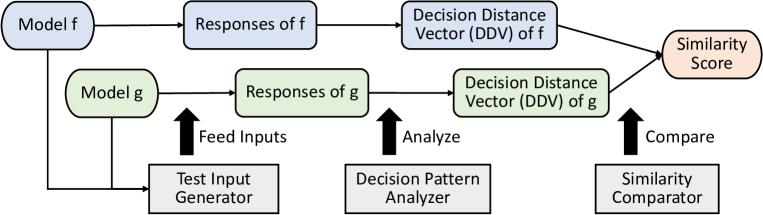
Figure 2. The pipeline of ModelDiff to measure knowledge similarity between two models.

The pipeline of knowledge similarity analysis in ModelDiff is shown in Figure 2. The main components of ModelDiff include a test input generator, a decision pattern analyzer, and a vector similarity comparator.

Given two DNN models $f$ and $g$, the test input generator first generates several input examples $X$ that can trigger diverse reactions in the models, then the input examples are grouped into pairs $\operatorname{\textit{XP}}$ fed into the $f$ and $g$ one by one. For each input example $x\in X$, we record the responses of both models to the input as $f(x)$ and $g(x)$. The overall decision logic of a model is represented as a decision distance vector ($\operatorname{\textit{DDV}}_{f}$ and $\operatorname{\textit{DDV}}_{g}$ for $f$ and $g$ respectively). Finally, the similarity between the two models is measured by computing the distance between their $\operatorname{\textit{DDV}}$s. The following subsections will explain the key components in detail.

4.2. Test Input Generation

The goal of test input generation is to create an input dataset that can capture the decision logic shared by DNN models that contain reused knowledge.

Given two models $f$ and $g$ under comparison, we first select one model (say $f$) as the target model, and another model ($g$) is the suspect model. In most model comparison scenarios, one of the models is white-box accessible (e.g. the IP owner’s model or a public pretrained model), which should be selected as the target model. A random one is selected if both models are black-box.

We assume there is a set of normal input samples $X_{seed}$ available for the target model $f$, which is reasonable since the model’s prediction APIs are available and the functionalities are usually known.

Directly using the normal inputs to extract the decision logic of the models is problematic for our purpose, since the normal inputs can only trigger normal knowledge that may be shared by unrelated models. For example, suppose $f$ and $g$ are two irrelevant image classifiers trained from scratch (i.e. there is no knowledge reuse between them), $x_{cat1}$ and $x_{cat2}$ are two normal images of cat and $x_{dog}$ is a normal image of dog, then it is highly possible that:

$$\operatorname{\textit{dist}}(f(x_{cat1}),f(x_{cat2}))\approx\operatorname{\textit{dist}}(g(x_{cat1}),g(x_{cat2}))\approx 0$$

$$\operatorname{\textit{dist}}(f(x_{cat1}),f(x_{dog}))\approx\operatorname{\textit{dist}}(g(x_{cat1}),g(x_{dog}))>0$$

which means that the reaction patterns of $f$ and $g$ on the normal inputs may be indistinguishable. Such similarity between the decision patterns is caused by the intrinsic features in the normal inputs and the commonly-agreed labels of them - such knowledge of normal inputs is implied in the datasets and is obtained by different (unrelated) models trained on the similar datasets.

Thus, to achieve our goal (model reuse detection), we ought to generate test inputs that can trigger the model-specific knowledge that is shared by models with knowledge reuse while not shared by any other unrelated models.

Inspired by prior work on adversarial attacks (Szegedy et al., 2013; Demontis et al., 2019; Rezaei and Liu, 2019) that discovered the imperfect decision boundaries are one of the main reasons for adversarial vulnerability, we attempt to address the input generation problem from the decision boundary perspective.

We argue that the decision boundaries of models with reused knowledge are similar. For example, in transfer learning, the decision boundary of the teacher model is copied into the student and fine-tuned on the student dataset. The fine-tuning will not alter the decision boundary significantly, instead, it only adjusts the decision boundary to fit the student dataset. Similarly, other model reuse methods like pruning and quantization are also designed to inherit the decision boundary rather than changing it. Thus, if we can precisely interpret the decision boundaries with the test inputs, it will help identify the reusing relation between DNNs.

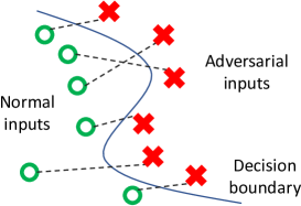
Figure 3. Illustration of the decision boundary depicted by normal and adversarial input pairs.

We combine adversarial inputs and normal inputs to create the test inputs in ModelDiff. The intuition behind this idea is shown in Figure 3. Specifically, for each normal input $x_{i}\in X$, we generate a corresponding adversarial input $x_{i}^{\prime}$ by adding small perturbation to $x_{i}$. The normal input $x_{i}$ usually lies inside the decision boundary, and the output produced by the normal input typically reflect the general knowledge shared by similar but unrelated models. The adversarial input $x_{i}^{\prime}$, on the other hand, lies around the decision boundary and the corresponding output is mainly determined by the model-specific imperfect decision boundary. By using each other as a reference, the decision distance between normal and adversarial inputs can convey the knowledge exclusively shared between reused models, i.e.

$$\operatorname{\textit{dist}}(f(x_{i}),f(x_{i}^{\prime}))\approx\operatorname{\textit{dist}}(g(x_{i}),g(x_{i}^{\prime})),\ if\ f\sim g$$

$$\operatorname{\textit{dist}}(f(x_{i}),f(x_{i}^{\prime}))\neq\operatorname{\textit{dist}}(g(x_{i}),g(x_{i}^{\prime})),\ if\ not\ f\sim g$$

To generate the adversarial inputs $X^{\prime}=\{x_{i}^{\prime},x_{2}^{\prime},...\}$ from the normal inputs $X=\{x_{i},x_{2},...\}$, we introduce two criteria to measure the quality of generated test inputs, including intra-input distance that represents the element-wise distance between the outputs produced by $X$ and $X^{\prime}$ and inter-input diversity that represents the diversity of outputs produced by $X^{\prime}$.

$$\operatorname{\textit{divergence}}_{f}(X^{\prime},X)=\operatorname*{\textit{mean}}_{i=0,1,...,|X|}\big{\{}||f(x_{i}^{\prime})-f(x_{i})||_{2}\big{\}}$$

$$\operatorname{\textit{diversity}}_{f}(X^{\prime})=\operatorname*{\textit{mean}}_{x^{\prime}_{i},x^{\prime}_{j}\in X^{\prime}}\big{\{}||f(x^{\prime}_{i})-f(x^{\prime}_{j})||_{2}\big{\}}$$

The implication is two-fold: First, $\operatorname{\textit{divergence}}_{f}(X^{\prime},X)$ implies the strength of the adversarial inputs, i.e. the decision boundary depicted by $X$ and $X^{\prime}$ are more transferable if $\operatorname{\textit{divergence}}$ is larger. Second, $\operatorname{\textit{diversity}}_{f}(X^{\prime})$ indicates the coverage of behaviors produced by the inputs. There are more standard neuron coverage metrics proposed by prior work (Pei et al., 2017; Ma et al., 2018a), but we use the output-based criteria $\operatorname{\textit{diversity}}_{f}(X^{\prime})$ since we don’t assume the access to the model internal structure. The quality score of a set of adversarial inputs $X^{\prime}$ is measured by:

(1) $$score(X^{\prime})=\operatorname{\textit{divergence}}_{f}(X^{\prime},X)+\lambda\>\operatorname{\textit{diversity}}_{f}(X^{\prime})$$

where $\lambda$ is a hyperparameter to balance the two criteria.

The goal of input generation is to find:

(2) $$\hat{X^{\prime}}=\operatorname*{arg\,max}_{X^{\prime}}\>score(X^{\prime})$$

There are several ways to solve Equation 2. If $f$ is white-box accessible, the adversarial inputs can be generated through gradient ascent (Madry et al., 2017; Szegedy et al., 2013). Specifically, we select a target output $f(X^{\prime})$ that maximizes Equation 2 and use the PGD attack (Madry et al., 2017) to generate $X^{\prime}$ that can minimize the loss between $f(X^{\prime})$ and $f(X)$.

In cases where the target model is also black-box, we introduce a criteria-guided search algorithm (as shown in Algorithm 1) to generate test inputs for the model $f$ by gradually mutating the seed inputs towards to the goal. The algorithm is inspired by prior work on mutation testing (Jia and Harman, 2010) and black-box adversarial attack (Guo et al., 2019; Demir et al., 2019) while tailored for our objective in terms of mutation index selection and mutation operation.

Input: $f$: the target model, $X$: the set of seed inputs, $\lambda$, $\epsilon$, $N$: hyperparameters to control divergence-diversity balance, mutation strength, and number of iterations.

1 initialize inputs $X^{\prime}\leftarrow X$

2 initialize $score\leftarrow\operatorname{\textit{divergence}}_{f}(X,X^{\prime})+\lambda\>\operatorname{\textit{diversity}}_{f}(X^{\prime})$

3 for $i$ from 1 to $N$ do

      4 compute $\operatorname{\textit{divergence}}_{f}(X,X^{\prime})$ and $\operatorname{\textit{diversity}}_{f}(X^{\prime})$

      5 $indices\leftarrow I_{low\_divergence}\>\bigcup\>I_{low\_diversity}$

      6 $pos\leftarrow random\_pick(X[0].shape)$

      7 compute $X^{\prime}_{left}$ by adding $-\epsilon$ to $X^{\prime}[indices][pos]$

      8 compute $X^{\prime}_{right}$ by adding $\epsilon$ to $X^{\prime}[indices][pos]$

      9 compute $score_{left}$ and $score_{right}$ using $X^{\prime}_{left}$ and $X^{\prime}_{right}$

      10 if $score_{left}>score$ and $score_{left}>score_{right}$ then

            11 $X^{\prime}\leftarrow X^{\prime}_{left}$, $score\leftarrow score_{left}$

      12 else if $score_{right}>score$ then

            13 $X^{\prime}\leftarrow X^{\prime}_{right}$, $score\leftarrow score_{right}$

      

14return the generated test inputs $X^{\prime}$

Algorithm 1 Black-box input generation in ModelDiff.

Given a target model $f$ and a set of seed inputs $X$, we generate the test inputs through $N$ mutating iterations. In each iteration, we select a subset of input samples (named mutation inputs) in $X$ that are the primary cause of low divergence and low diversity (line 6). $I_{low\_divergence}$ are the indices of inputs where each $j\in I_{low\_divergence}$ satisfies $||f(x^{\prime}_{j})-f(x_{j})||_{2}<\operatorname{\textit{divergence}}_{f}(X,X^{\prime})$, i.e. the divergence between $x_{j}$ and $x^{\prime}_{j}$ is lower than the average thus $x^{\prime}_{j}$ should be mutated. To compute $I_{low\_diversity}$, we first calculate the distance $||f(x^{\prime}_{j})-f(x^{\prime}_{k})||_{2}$ between each input pair $x_{k},x_{l}\in X^{\prime}$. The input pairs with smaller distances are more responsible for the low diversity thus should be mutated. We set $I_{low\_diversity}$ to the indices of the first $r\times n$ input pairs, where $r$ is a hyperparameter to control the size of $I_{low\_diversity}$. $r$ is set to 0.5 by default so that $I_{low\_diversity}$ will contain no more than $n/2$ indices.

After selecting the mutation inputs, we randomly pick a position $pos$ in the input shape (e.g. a pixel in the input image) to perform the mutation operation. We obtain two sets of inputs $X^{\prime}_{left}$ and $X^{\prime}_{right}$ that are generated by adding a small perturbation $\epsilon$ to or subtracting $\epsilon$ from the mutation position $pos$ in each mutation input. We compute the scores for $X^{\prime}_{left}$ and $X^{\prime}_{right}$ respectively with Equation 1 and update the test input set $X^{\prime}$ if the score is improved. The mutation process is repeated for $N$ iterations and the final input set $X^{\prime}$ is produced as the result of input generation.

4.3. Similarity Comparison

With the normal seed inputs $X$ and adversarial inputs $X^{\prime}$ generated in Section 4.2, we are able to compute the decision distance vectors (DDVs) for the models under comparison.

First, the normal inputs $X$ and adversarial inputs $X^{\prime}$ are combined to form a list of input pairs $\operatorname{\textit{XP}}=\{(x_{1},x_{1}^{\prime}),(x_{2},x_{2}^{\prime}),...,(x_{n},x_{n}^{\prime})\}$, where $x_{i}\in X$, $x_{i}^{\prime}\in X^{\prime}$, and $n$ is the number of inputs in $X$. The decision distance vector (DDV) is defined as:

Definition 0.

(Decision distance vector) Given a list of input pairs $\operatorname{\textit{XP}}$, the decision distance vector (DDV) of a model $f$ is a float vector $\operatorname{\textit{DDV}}_{f}(\operatorname{\textit{XP}})=<v_{1},v_{2},...,v_{n}>$, in which each element $v_{i}=\operatorname{\textit{dist}}(f(x_{i}),f(x_{i}^{\prime}))$ is the distance between the responses of $f$ produced by $x_{i}$ and $x_{i}^{\prime}$.

For each input pair, DDV measures the distance between the outputs produced by the two inputs. Since the outputs are produced by the same model, the outputs $f(x_{i})$ and $f(x_{i}^{\prime})$ are comparable. The distance metric $\operatorname{\textit{dist}}$ is the Cosine distance here if $f(x_{i})$ is a 1-D array (e.g. when $f$ is a classifier), since Cosine distance is good at comparing different scales of vectors.

A DDV basically captures the decision pattern of a model on the test inputs. If two models are similar, they would have similar patterns when measuring the distance between each pair of test inputs. The concept is analogous to testing two people with the same quiz questions, they would give similar answers if they have common knowledge.

The length of DDV equals to the number of input pairs in $\operatorname{\textit{XP}}$ used to compute the DDV. By using the same set of profiling input pairs to compute the DDVs for different models, we are able to generate DDVs with fixed length and common semantics. Thus the DDVs are comparable across different models, and the model similarity can be measured through DDV comparison. Specifically,

$$\operatorname{\textit{sim}}(f,g)=Cosine\_similarity(\operatorname{\textit{DDV}}_{f},\operatorname{\textit{DDV}}_{g})$$

4.4. Threshold to Identify Model Reuse

The similarity score computed by ModelDiff is an indicator of how likely a model is reused from another. However, in practice it is usually desirable to have a threshold to decide whether it is a reuse. Defining a global threshold is difficult because the range of similarity scores may differ across various model types. Instead, we opt for a data-driven model-specific threshold, i.e. when we want to determine whether a suspect model $g$ is a reuse of the target model $f$, we first collect (or generate) several reference models that are similar to $f$ but not built upon $f$ (e.g. models trained with the same dataset of $f$ from scratch or built upon other pretrained models). Then the threshold can be determined as the maximum of the similarity scores obtained by the reference models. We will show in Section 5.2 that such threshold is feasible and effective.

5. Evaluation

Our evaluation aims to address the following research questions:

1. What is the performance of ModelDiff? Is it able to correctly detect different types of model reuses? (§5.2)

2. How effective are the inputs generated with mutations in the complete black-box setting? (§5.3)

3. How do different configurations of ModelDiff affect the similarity comparison performance? (§5.4)

4. Can ModelDiff be applied to real-world deep learning apps to analyze model similarity? (§5.5)

5.1. Experiment Setup

The ModelReuse Benchmark. To evaluate our method, we create a benchmark named ModelReuse for model similarity comparison.

We use state-of-the-art image classification models and datasets that commonly appear in transfer learning literature to construct the benchmark. The source models to transfer knowledge from are ResNet18 (He et al., 2016) and MobileNetV2 (Sandler et al., 2018) pretrained on ImageNet (Deng et al., 2009), and the datasets to transfer knowledge into are Oxford Flowers 102 (Flower102 for short) (Nilsback and Zisserman, 2008) and Stanford Dogs 120 (Dog120 for short) (Khosla et al., 2011). The other models are generated from the base models using different model reuse methods with varying configurations.

Table 2. The 114 models included in ModelReuse benchmark. The pretrained models are downloaded from the Internet. The transferred models are built upon the pretrained models. The pruned/quantized/distilled/stolen models are based on the transferred models. The retrained models are built from scratch. The “#” column is the number of models trained with the corresponding method and configuration, and the “Examples” column shows the names of some models in the category.

Method	Configuration	#	How to generate	Examples
Pre-training	-	2	6.8cm- Train ResNet18 and MobileNetV2 on ImageNet dataset.	7cmtrain(ResNet)
train(MbNet)
Transfer learning	Tune 10% layer	4	- Transfer each source model to each target dataset (Flower102 and Dog120), fine-tune the last 10% layers.	train(ResNet)-transfer(Flower102,0.1)
	Tune 50% layers	4	- Transfer each source model to each target dataset, fine-tune the last 50% layers.	train(MbNet)-transfer(Dog120,0.5)
	Tune all layers	4	- Transfer each source model to each target dataset, fine-tune all 100% layers.	train(MbNet)-transfer(Dog120,1.0)
Pruning	Prune ratio 0.2	12	- Prune 20% weights in each transferred model and fine-tune.	train(ResNet)-transfer(Dog120,0.5)-prune(0.2)
	Prune ratio 0.5	12	- Prune 50% weights in each transferred model and fine-tune.	train(MbNet)-transfer(Flower102,0.1)-prune(0.5)
	Prune ratio 0.8	12	- Prune 80% weights in each transferred model and fine-tune.	train(ResNet)-transfer(Dog120,1.0)-prune(0.8)
Quantization	INT8	12	- Compress each transferred model using post-training weight quantization.	train(ResNet)-transfer(Flower102,0.1)-quant
Knowledge distillation	same arch	12	- Distill each transferred model to a target model with the same architecture using feature distillation.	train(MbNet)-transfer(Dog120,0.5)-distill
Stealing	different arch	12	- Use the output of each transferred model to train a target model with different architecture.	train(ResNet)-transfer(Flower102,0.5)-steal(MbNet)
Retraining	-	28	6.8cm- Train ResNet18 and MobileNetV2 on each target dataset from scratch. Use model reuse techniques to generate more variations.	7cmretrain(ResNet)
retrain(MbNet)-transfer(Flower102,0.5)

The complete list of models included in ModelReuse is shown in Table 5.1. In total we have 114 models, including 2 pretrained source models, 84 student models (12 transferred + 36 pruned + 12 quantized + 12 distilled + 12 stolen), and 28 retrained models. Each of the 84 student models is built from one of the two pretrained source models, and the 28 retrained models are trained from scratch.

Based on the models, we obtain 144 pairs of similar models (i.e. model pairs in which one model reuses the knowledge of another model, and should be detected as similarity), including 84 direct-reuse model pairs and 60 combined-reuse model pairs. Each direct-reuse model pair is a student model with its direct teacher model. Each of the 60 combined-reuse model pairs is generated with a combination of two reuse methods (transfer learning + model compression) from the corresponding source model. Such combined reuse is common in real-world deep learning applications where both the task and the model size are customized.

Baselines. To our best knowledge, there is no existing work aimed to address the same problem as ours. However, there are similar concepts discussed in related fields such as transfer learning, watermarking, etc. Thus we implement several baselines for comparison:

1. WeightCompare measures the model similarity directly based on weight comparison. Specifically, the similarity between model $f$ and $g$ is calculated by $\frac{\#\text{identical layers between f and g}}{min(\#\text{layers of f},\ \#\text{layers of g})}$, where two layers are identical if and only if their structures and weights are the same.

2. FeatureCompare compares the feature maps produced by the same set of $N$ normal inputs. Suppose $f^{feat}(x)$ is the feature map of the last Conv layer in model $f$ produced by input $x$, then the model similarity between $f$ and $g$ is calculated by $mean_{i=1}^{N}\{cosine(f^{feat}(x_{i}),g^{feat}(x_{i}))\}$.

3. Fingerprinting computes a fingerprint of the teacher model and check the fingerprint against other models to measure similarity. The idea (Cao et al., 2019; Lukas et al., 2019) is to fingerprint a model $f$ with a set of adversarial inputs $X$ and their predicted label $Y_{f}$. Given a new model $g$, the IP ownership is verified by checking whether $Y_{g}\approx Y_{f}$. We use the same inputs as ours to compute fingerprints and calculate model similarity as $sim(Y_{f},Y_{g})$.

WeightCompare and FeatureCompare are while-box methods since they require reading the weights or feature maps. Fingerprinting is a black-box method like ours. We also considered other baselines such as directly comparing the model outputs (OutputCompare), but since Fingerprinting is also based on output comparison, it should be able to represent the performance of OutputCompare.

Implementation and Test Environment. ModelDiff was implemented with PyTorch 1.3 and Tensorflow 2.0 using Python 3.6. Unless otherwise noted, we assume the target model is white-box accessible and the suspect model is black-box, and the test inputs are generated using gradient ascent. The number of test inputs was set to 100 and the hyperparameters $\lambda$, $\epsilon$ and $N$ were set to 0.5, 0.06, and 20,000 by default in our implementation. The benchmark dataset was generated on a GPU cluster, and the experiments were conducted on a Linux Server with 2 Intel Xeon CPUs and 2 GeForce GTX 1080Ti GPUs. It takes around 18 seconds for ModelDiff to compare a pair of models.

5.2. Correctness on ModelReuse Benchmark

Table 3. The similarity comparison result of ModelDiff and other baselines on ModelReuse benchmark. Feas. and corr. are the abbreviations of feasibility and correctness respectively.

Reuse method		#Models	WeightCompare		FeatureCompare		Fingerprinting		ModelDiff (ours)
			Feas.	Corr.	Feas.	Corr.	Feas.	Corr.	Feas.	Corr.
Direct reuse	Transfer - tune 10%	4	✓	100%	✓	100%	✗	-	✓	100%
	Transfer - tune 50%	4	✓	100%	✓	100%	✗	-	✓	100%
	Transfer - tune 100%	4	✓	0%	✓	100%	✗	-	✓	100%
	Prune 20%	12	✓	0%	✓	100%	✓	100%	✓	100%
	Prune 50%	12	✓	0%	✓	100%	✓	100%	✓	100%
	Prune 80%	12	✓	0%	✓	100%	✓	66.7%	✓	100%
	Quantize	12	✓	100%	✓	100%	✓	100%	✓	100%
	Distill - same arch	12	✓	0%	✓	50.0%	✓	75.0%	✓	100%
	Steal - different arch	12	✗	-	✗	-	✓	0%	✓	0%
Combined reuse	Transfer + prune	36	✓	0%	✓	100%	✗	-	✓	100%
	Transfer + quantize	12	✓	66.7%	✓	100%	✗	-	✓	100%
	Transfer + distill	12	✓	0%	✓	50.0%	✗	-	✓	100%
Overall		144	91.7%	21.2%	91.7%	90.9%	50.0%	73.6%	100%	91.7%

We first ran ModelDiff and the baseline methods on the ModelReuse benchmark to test their performance of similarity comparison.

For each of the 144 reused model pairs in ModelReuse, we generate reference model pairs by randomly replacing one of the two models with an unrelated one (e.g. a model with different source model or a retrained model). Thus each reused model pair has 71 reference model pairs. When evaluating a model comparison method, each reused model pair and its corresponding reference model pairs are fed into the comparator, and the following two metrics are computed for each method: Feasibility. Whether the comparator can be used to compare the reused model pair. Correctness. Whether the comparator can distinguish the reused model pair from reference model pairs (i.e. whether the similarity score of the reused model pair is higher than all reference model pairs).

The results are shown in Table 3. First of all, ModelDiff achieved 100% feasibility, meaning that ModelDiff can measure the similarity between all types of models, including those with different model architectures or output spaces, while all other baselines are not 100% feasible. Specifically, the white-box approaches are unable to process models with different architecture, which is a disadvantage since the cross-structure distillation techniques (Hinton et al., 2015) are gaining popularity. Fingerprinting is not designed for models with different underlying tasks, thus was unable to detect any reuse related to transfer learning.

ModelDiff achieved overall correctness of 91.7%, outperforming all the other baseline methods including the white-box approach FeatureCompare. Specifically, ModelDiff was able to precisely identify the reused models generated with all model reuse methods except for stealing. FeatureCompare is also precise on most normal reuses. However, the qualitative differences between FeatureCompare and ModelDiff are notable. First, FeatureCompare is a white-box approach because it requires access to the intermediate feature of the compared models. Second, FeatureCompare assumes that the compared models have a common feature layer for comparison. However, finding the common layer between two models is non-trivial or even impossible, especially if the suspect model is generated through knowledge distillation or modified purposely. Table 3 has showed that FeatureCompare was not as effective on models generated with knowledge distillation that may lead to significant internal feature change by retraining the weights from scratch.

The stolen models were difficult to detect with all methods. Stealing a model is almost equivalent to retraining it, and the teacher model is only used to generate a training dataset. How to identify models generated with stealing remains a challenging problem.

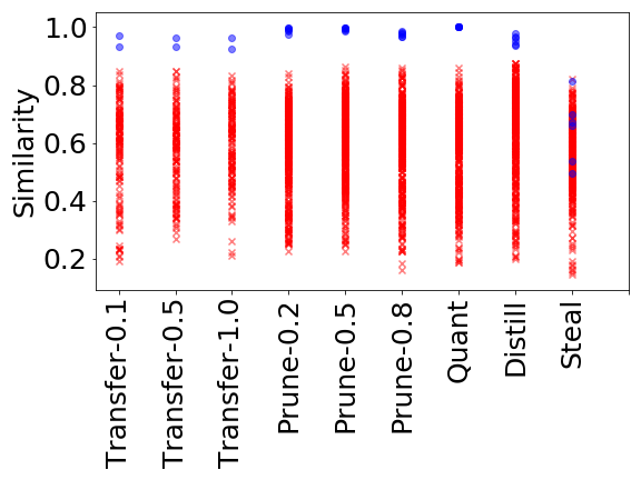
Figure 4. The similarity score distribution of different reuse methods. Blue dots and red crosses are the similarity scores obtained by reused models and irrelevant models respectively.

Figure 4 shows the distribution of the similarity scores computed by ModelDiff on the ResNet-based models. In most model reuse cases that ModelDiff can correctly detect, we observe a clear gap between the scores achieved by the reused model pairs and the reference model pairs, meaning it’s easy to identify reused models with a threshold. The gap is smaller when the models are generated with knowledge distillation, which is intuitive since distillation would reset the model parameters rather than reuse the parameters from the teacher, thus less decision boundaries are inherited.

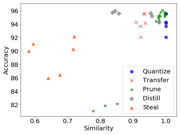
Figure 5. Relation between model similarity and test accuracy on Flower102 dataset.

To further interpret the similarity scores, we visualized the relation between each student model’s similarity score and its test accuracy in Figure 5. We noticed that the student models with higher accuracy typically have higher similarity scores, because more useful knowledge is transferred from the teacher. The test accuracy of the models generated with stealing attack is lower, meaning that they didn’t reuse much useful knowledge although they are harder to detect. Surprisingly, although some models (pruning 80% weights in MobileNet) didn’t inherit much useful knowledge from the teacher (thus had a poor accuracy), we are still able to correctly detect them.

5.3. Complete Black-box Setting

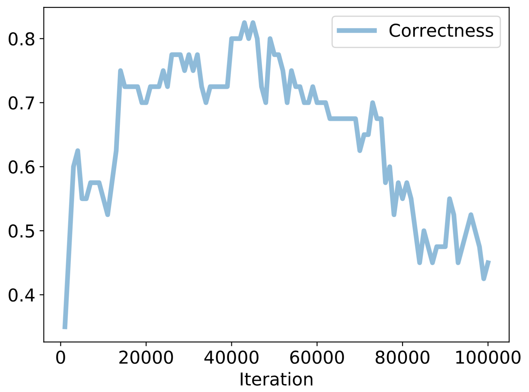
Figure 6. Progressive correctness achieved with different numbers of input mutations in complete black-box setting.

In complete black-box settings, both models under comparison are black-box. Thus the test inputs can only be generated with mutation (Algorithm 1) rather than gradient ascent. To evaluate the performance of ModelDiff in this setting, we used the two pretrained models (ResNet18 and MobileNetV2) to generate test inputs, and measured the correctness achieved by the generated inputs every 1,000 iterations. The result is shown in Figure 6.

At first, the correctness improved quickly as more mutations were performed, since the generated inputs became better at depicting the decision boundaries. The correctness went to 70%-80% with roughly 20,000 to 60,000 mutations (which took around 1-3 hours), meaning that ModelDiff was able to measure model similarity with a reasonable accuracy in complete black-box settings. However, the correctness started to drop when the number of mutations was larger, because too many mutations had made the adversarial inputs more transferable to other irrelevant models. In practice, we should limit the number of mutations to avoid such issues. We leave more stable and effective black-box generation of adversarial inputs that are only transferable to reused models as future work.

5.4. Configuration Analysis

Table 4. The relative correctness of ModelDiff under different configurations as compared to the default setting.

Variation	Relative correctness
Random noise as seed inputs	0.59
Less (10) or more (200) seed inputs	0.82, 1.00
Irrelevant images as seed inputs	1.00
All normal inputs	0.61
All adversarial inputs	0.86
Without diversity	0.75

Since the test inputs are critical in ModelDiff to precisely measure the knowledge similarity, we further analyzed how different configurations of test inputs may affect the correctness on the 84 direct-reuse model pairs. The results are shown in Table 4.

The first three rows discuss the choice of seed inputs. The choice of seed inputs is important for ModelDiff since using random noises as the seed inputs or reducing the number of seed inputs would lead to a correctness drop. However, ModelDiff performs well even if the seed inputs are irrelevant images drawn from other datasets. Thus ModelDiff only requires the inputs to comply with the input distribution of the models under comparison.

The following two rows discuss how effective it is to measure model similarity with normal inputs only or adversarial inputs only. Both the two variations were unable to achieve performance comparable to our default configuration (half adversarial inputs and half normal inputs), which demonstrates the effectiveness of ModelDiff in using adversarial inputs and corresponding normal inputs together to interpret the models’ decision boundaries.

The last row discusses the usefulness of the diversity metric introduced in Section 4.2. By removing the diversity of seed inputs and disabling the diversity criterion in Equation 1, ModelDiff’s overall correctness dropped by 25%. This demonstrates the usefulness of considering test output diversity when generating test inputs.

5.5. A Study on Real-world Models

We further studied whether ModelDiff can be applied to measure similarity for real-world models by testing it on models extracted from real-world Android apps.

We selected MobileNet-V2 (Sandler et al., 2018) pretrained on ImageNet (Deng et al., 2009) as the source model due to its popularity in mobile apps. The pretrained MobileNet-V2 was obtained from Keras (https://keras.io/), which is commonly used by app developers to download pretrained models. The test inputs used by ModelDiff to measure knowledge similarity were generated from the source model.

To obtain real-world models, we crawled 20,000 popular apps from Google Play and looked for DNN models contained in those apps. We focused on TFLite models since TFLite is the most popular mobile deep learning framework today and .tflite model files are self-contained and suitable for automated analysis. In the end, we obtained 149 apps that contain at least a TFLite model. By excluding the models whose input shape was different from the source model, we obtained 35 models for comparison.

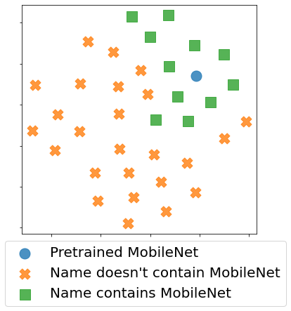
Figure 7. t-SNE visualization of the DDVs computed for 35 real-world mobile deep learning models.

All the 35 models were successfully processed by ModelDiff to compute DDVs with the test inputs. Since there is no ground truth about whether each model is similar with the source model, we were unable to compute the correctness like in Section 5.2. Instead, we grouped the models into two categories based on whether the model name contains “MobileNet” and examined whether the DDVs computed for the models with “MobileNet” in name are closer to the source model. The result shows that the DDVs of similar models (e.g. the MobileNet-related models) are grouped close to each other, which demonstrates the effectiveness of using DDVs to measure model similarity. Such clustering ability of ModelDiff can potentially be used to analyze model reuse relations at scale in an unsupervised manner.

6. Related work

6.1. Software Similarity Comparison

Our work is partly inspired by the line of research on code similarity analysis, which has a long history since the emergence of computer software (Ragkhitwetsagul et al., 2018; Rattan et al., 2013). Existing work can be roughly classified into metrics-based, text-based, graph-based, and semantic-based approaches. The metrics-based approaches (Ottenstein, 1976; Berghel and Sallach, 1984) are mainly focused on computing some metrics from the software and measure the similarity by comparing the metrics. Text-based approaches (Roy and Cordy, 2008; Li et al., 2006; Schleimer et al., 2003; Guo et al., 2018) view the code snippets as string sequences and compare them using text similarity analysis techniques. Graph-based approaches parse the programs into a uniform structure (such as abstract syntax tree (Baxter et al., 1998), control flow graph (Chae et al., 2013), program dependence graph (Krinke, 2001), UI transition graph (Li et al., 2017), etc.) and identify isomorphism between the trees or graphs. Some recent approaches consider the semantics of code during similarity detection, with the help of advanced NLP and ML techniques (McMillan et al., 2012; Xu et al., 2017; Liu et al., 2018a).

In cybersecurity research, binary code similarity comparison is attractive due to its rich applications in patch analysis, plagiarism detection, malware detection, and vulnerability search (Haq and Caballero, 2019; Ding et al., 2019; Ming et al., 2017; Xu et al., 2017). Jiang et al. ’s work (Jiang and Su, 2009) is the closest to ours, which proposed to compare the final states of two pieces of binary code given the same input. If the pieces of code produce the same output, they are considered equivalent. The same idea is later used in BLEX (Egele et al., 2014) and MULTI-MH (Pewny et al., 2015) for binary similarity detection. Although the testing-based concept is similar to ours, we deal with DNN models that may serve different tasks.

DNN model similarity has also been discussed in the AI and machine learning field (Morcos et al., 2018; Raghu et al., 2017; Kornblith et al., 2019). The main method is canonical correlation analysis (CCA) and the primary purpose is to understand the model internal representation rather than detect reuse. Thus we did not compare with these approaches in this paper.

6.2. Model Intellectual Property Protection

To protect the IP right of a model, one way is to avoid model exposure by encrypting it (Gilad-Bachrach et al., 2016), putting it or part of it into enclaves (Tramer and Boneh, 2018; Zhang et al., 2020b), etc. Another way is to design mechanisms to enable model IP violation detection. Here we focus on the detection approaches, including watermarking and fingerprinting.

A watermark for a DNN model is usually a marker covertly embedded into the model’s weight or output. Weight watermarks (Uchida et al., 2017; Chen et al., 2019a, b) are usually trained into the weights using a parameter regularizer and verified by directly comparing the weights of the intermediate layers. Output watermarks (Adi et al., 2018; Darvish Rouhani et al., 2019; Fan et al., 2019) are generated by training the DNN model to predict certain outputs (or activation values) on specific inputs, like a backdoor injected into the model. These approaches have in common that the models are overfitted on certain inputs, i.e. the watermarks are additional knowledge inserted into the model rather than the intrinsic knowledge of the model. Recent studies have found that the watermarks are not robust against distillation (Shafieinejad et al., 2019) and retraining (Aiken et al., 2021).

Unlike watermarking, fingerprinting approaches are focused on post hoc detection of model reuse. For example, IPGuard (Cao et al., 2019) is based on the observation that a DNN classifier can be uniquely represented by its classification boundary. Specifically, they find N data points around the classification boundary and use the data points together with the predicted labels as the fingerprint. A suspect model is examined by feeding the N data points and comparing the predicted labels. An IP violation is detected if the suspect model produces outputs similar to the source model. Lukas et al. (Lukas et al., 2019) introduced the concept of conferrable inputs, i.e. targeted adversarial inputs that are transferable to surrogate models while not transferable to reference models that are trained independently. A major limitation of these approaches is that the outputs of source and suspect model must be in the same label space in order to verify the ownership, which is not true since the suspect models may be transferred to different tasks.

The DDV in this paper can also be viewed as a model fingerprint. However, our method has more broad applicability since we do not require the models to have the same output space.

6.3. Test Input Generation for DNN

Prior to our work, DNN testing has been widely discussed (Zhang et al., 2020a). The primary goal of test input generation for DNNs is to measure or improve the robustness of models to adversarial inputs. For example, DeepXplore (Pei et al., 2017) introduced the concept of neuron coverage, i.e. the ratio of neurons activated by a set of inputs, to describe the adequacy of the input set in revealing the possible behaviors of the model. DeepGauge (Ma et al., 2018a) then extended the concept by considering more fine-grained criteria. Various searching, mutating, and fuzzing techniques (Tian et al., 2018; Odena et al., 2019; Xie et al., 2019) have also been proposed to generate test inputs that can maximize the coverage metrics.

There are also other purposes of DNN testing. For example, Ma et al.  (Ma et al., 2018b) proposed to debug model bugs. Zhang et al.  (Zhang et al., 2020c) and Aggarwal et al.  (Aggarwal et al., 2019) attempted to test model fairness. Tian et al.  (Tian et al., 2019) are focused on testing the confusion and bias errors in DNNs. In this work, DNN testing is used for model reuse detection.

7. Limitations and Future Work

Other Reuse Methods. There are many novel model reuse methods and many variations of existing model reuse methods introduced every day. It is impossible to test all of them, and we only considered the most representative and widely-used ones.

Models generated with other reuse methods may bypass our detection, especially if the student model developers are malicious and aware of our method. How to deal with malicious model reuse methods (e.g. model stealing attack) still remains a open problem. More fundamentally, how to rigorously define DNN knowledge reuse and detect any form of it is an important direction to explore.

Models with Different Input Shapes. Since our method requires testing the models under comparison with the same set of inputs, it is not able to measure similarity for models with different input shapes. Fortunately, in most model reuse cases, the models with different input shapes are unlikely to be built from each other.

Other Model Types. Currently ModelDiff is only tested on CNN models, while we believe the idea of interpreting a precise and complete decision boundary is general across different types of models. In the future we will try to adapt our method to other types of models such as RNN and Transformers.

Distinguishing Teacher and Student. ModelDiff currently does not distinguish the direction of model reuse, i.e. we are unable to know which is the teacher model and which is the student given two models with knowledge similarity. The ability to detect the reuse direction would be important when one needs to decide the IP ownership among similar models.

8. Conclusion

This paper introduces a method named ModelDiff for measuring knowledge similarity between DNN models. The idea is based on the insight that models with similar knowledge would group a set of inputs in similar patterns, and the decision boundaries of a model depicted by normal and adversarial input pairs are transferable to its student models. Experiments have shown that our method can achieve a high correctness on our benchmark built with popular model reuse techniques. The source code is available at https://github.com/ylimit/ModelDiff.

Acknowledgments

We thank all anonymous reviewers for the valuable comments. This work is done while Yunxin Liu was working at Microsoft and Ziqi Zhang was an intern at Microsoft. Ziqi Zhang contributed equally as a co-primary author. Yuanchun Li is the corresponding author.

References

- (1)
- Adi et al. (2018) Yossi Adi, Carsten Baum, Moustapha Cisse, Benny Pinkas, and Joseph Keshet. 2018. Turning your weakness into a strength: Watermarking deep neural networks by backdooring. In 27th USENIX Security Symposium (USENIX Security 18). 1615–1631.
- Aggarwal et al. (2019) Aniya Aggarwal, Pranay Lohia, Seema Nagar, Kuntal Dey, and Diptikalyan Saha. 2019. Black box fairness testing of machine learning models. In Proceedings of the 2019 27th ACM Joint Meeting on European Software Engineering Conference and Symposium on the Foundations of Software Engineering. 625–635. https://doi.org/10.1145/3338906.3338937
- Aiken et al. (2021) William Aiken, Hyoungshick Kim, Simon Woo, and Jungwoo Ryoo. 2021. Neural network laundering: Removing black-box backdoor watermarks from deep neural networks. Computers & Security 106 (2021), 102277. https://doi.org/10.1016/j.cose.2021.102277
- Baxter et al. (1998) Ira D Baxter, Andrew Yahin, Leonardo Moura, Marcelo Sant’Anna, and Lorraine Bier. 1998. Clone detection using abstract syntax trees. In Proceedings. International Conference on Software Maintenance (Cat. No. 98CB36272). IEEE, 368–377.
- Berghel and Sallach (1984) H. L. Berghel and D. L. Sallach. 1984. Measurements of Program Similarity in Identical Task Environments. SIGPLAN Not. 19, 8 (Aug. 1984), 65–76. https://doi.org/10.1145/988241.988245
- Cao et al. (2019) Xiaoyu Cao, Jinyuan Jia, and Neil Zhenqiang Gong. 2019. IPGuard: Protecting the Intellectual Property of Deep Neural Networks via Fingerprinting the Classification Boundary. arXiv preprint arXiv:1910.12903 (2019).
- Chae et al. (2013) Dong-Kyu Chae, Jiwoon Ha, Sang-Wook Kim, BooJoong Kang, and Eul Gyu Im. 2013. Software Plagiarism Detection: A Graph-Based Approach. In Proceedings of the 22nd ACM International Conference on Information & Knowledge Management (San Francisco, California, USA) (CIKM ’13). Association for Computing Machinery, New York, NY, USA, 1577–1580. https://doi.org/10.1145/2505515.2507848
- Chen et al. (2019a) Huili Chen, Cheng Fu, Bita Darvish Rouhani, Jishen Zhao, and Farinaz Koushanfar. 2019a. DeepAttest: An end-to-end attestation framework for deep neural networks. In 2019 ACM/IEEE 46th Annual International Symposium on Computer Architecture (ISCA). IEEE, 487–498. https://doi.org/10.1145/3307650.3322251
- Chen et al. (2019b) Huili Chen, Bita Darvish Rouhani, Cheng Fu, Jishen Zhao, and Farinaz Koushanfar. 2019b. Deepmarks: A secure fingerprinting framework for digital rights management of deep learning models. In Proceedings of the 2019 on International Conference on Multimedia Retrieval. 105–113. https://doi.org/10.1145/3323873.3325042
- Coleman et al. (2017) Cody Coleman, Deepak Narayanan, Daniel Kang, Tian Zhao, Jian Zhang, Luigi Nardi, Peter Bailis, Kunle Olukotun, Chris Ré, and Matei Zaharia. 2017. Dawnbench: An end-to-end deep learning benchmark and competition. Training 100, 101 (2017), 102.
- Dansplaining (2018) Dansplaining. 2018. How much did AlphaGo Zero cost? https://www.yuzeh.com/data/agz-cost.html.
- Darvish Rouhani et al. (2019) Bita Darvish Rouhani, Huili Chen, and Farinaz Koushanfar. 2019. DeepSigns: An end-to-end watermarking framework for ownership protection of deep neural networks. In Proceedings of the Twenty-Fourth International Conference on Architectural Support for Programming Languages and Operating Systems. 485–497. https://doi.org/10.1145/3297858.3304051
- Davchev et al. (2019) Todor Davchev, Timos Korres, Stathi Fotiadis, Nick Antonopoulos, and Subramanian Ramamoorthy. 2019. An empirical evaluation of adversarial robustness under transfer learning. In ICML workshop on understanding and improving generalization in deep learning.
- Demir et al. (2019) Samet Demir, Hasan Ferit Eniser, and Alper Sen. 2019. DeepSmartFuzzer: Reward Guided Test Generation For Deep Learning. arXiv preprint arXiv:1911.10621 (2019).
- Demontis et al. (2019) Ambra Demontis, Marco Melis, Maura Pintor, Matthew Jagielski, Battista Biggio, Alina Oprea, Cristina Nita-Rotaru, and Fabio Roli. 2019. Why do adversarial attacks transfer? explaining transferability of evasion and poisoning attacks. In 28th USENIX Security Symposium (USENIX Security 19). 321–338.
- Deng et al. (2009) Jia Deng, Wei Dong, Richard Socher, Li-Jia Li, Kai Li, and Li Fei-Fei. 2009. Imagenet: A large-scale hierarchical image database. In IEEE conference on computer vision and pattern recognition. IEEE, 248–255. https://doi.org/10.1109/CVPR.2009.5206848
- Ding et al. (2019) Steven HH Ding, Benjamin CM Fung, and Philippe Charland. 2019. Asm2vec: Boosting static representation robustness for binary clone search against code obfuscation and compiler optimization. In 2019 IEEE Symposium on Security and Privacy (SP). IEEE, 472–489. https://doi.org/10.1109/SP.2019.00003
- Dong et al. (2019) Yinpeng Dong, Tianyu Pang, Hang Su, and Jun Zhu. 2019. Evading Defenses to Transferable Adversarial Examples by Translation-Invariant Attacks. In IEEE conference on computer vision and pattern recognition (CVPR). Computer Vision Foundation / IEEE, 4312–4321. https://doi.org/10.1109/CVPR.2019.00444
- Egele et al. (2014) Manuel Egele, Maverick Woo, Peter Chapman, and David Brumley. 2014. Blanket execution: Dynamic similarity testing for program binaries and components. In 23rd USENIX Security Symposium (USENIX Security 14). 303–317.
- Fan et al. (2019) Lixin Fan, Kam Woh Ng, and Chee Seng Chan. 2019. Rethinking deep neural network ownership verification: Embedding passports to defeat ambiguity attacks. In Advances in Neural Information Processing Systems. 4714–4723.
- Gilad-Bachrach et al. (2016) Ran Gilad-Bachrach, Nathan Dowlin, Kim Laine, Kristin Lauter, Michael Naehrig, and John Wernsing. 2016. Cryptonets: Applying neural networks to encrypted data with high throughput and accuracy. In International Conference on Machine Learning. PMLR, 201–210. https://doi.org/10.5555/3045390.3045413
- Goodfellow et al. (2014) Ian J Goodfellow, Jonathon Shlens, and Christian Szegedy. 2014. Explaining and harnessing adversarial examples. arXiv preprint arXiv:1412.6572 (2014).
- Gu et al. (2017) Tianyu Gu, Brendan Dolan-Gavitt, and Siddharth Garg. 2017. Badnets: Identifying vulnerabilities in the machine learning model supply chain. arXiv preprint arXiv:1708.06733 (2017).
- Guo et al. (2019) Chuan Guo, Jacob R Gardner, Yurong You, Andrew Gordon Wilson, and Kilian Q Weinberger. 2019. Simple black-box adversarial attacks. arXiv preprint arXiv:1905.07121 (2019).
- Guo and Potkonjak (2018) Jia Guo and Miodrag Potkonjak. 2018. Watermarking deep neural networks for embedded systems. In 2018 IEEE/ACM International Conference on Computer-Aided Design (ICCAD). IEEE, 1–8. https://doi.org/10.1145/3240765.3240862
- Guo et al. (2018) Yao Guo, Yuanchun Li, Ziyue Yang, and Xiangqun Chen. 2018. What’s inside My App? Understanding Feature Redundancy in Mobile Apps. In Proceedings of the 26th Conference on Program Comprehension (Gothenburg, Sweden) (ICPC ’18). Association for Computing Machinery, New York, NY, USA, 266–276. https://doi.org/10.1145/3196321.3196329
- Han et al. (2015a) Song Han, Huizi Mao, and William J Dally. 2015a. Deep compression: Compressing deep neural networks with pruning, trained quantization and huffman coding. arXiv preprint arXiv:1510.00149 (2015).
- Han et al. (2015b) Song Han, Jeff Pool, John Tran, and William Dally. 2015b. Learning both weights and connections for efficient neural network. In Advances in neural information processing systems. 1135–1143.
- Haq and Caballero (2019) Irfan Ul Haq and Juan Caballero. 2019. A Survey of Binary Code Similarity. arXiv preprint arXiv:1909.11424 (2019).
- He et al. (2016) Kaiming He, Xiangyu Zhang, Shaoqing Ren, and Jian Sun. 2016. Deep residual learning for image recognition. In Proceedings of the IEEE conference on computer vision and pattern recognition. 770–778.
- Hinton et al. (2015) Geoffrey Hinton, Oriol Vinyals, and Jeff Dean. 2015. Distilling the knowledge in a neural network. arXiv preprint arXiv:1503.02531 (2015).
- Huang et al. (2019) Qian Huang, Isay Katsman, Horace He, Zeqi Gu, Serge Belongie, and Ser-Nam Lim. 2019. Enhancing adversarial example transferability with an intermediate level attack. In Proceedings of the IEEE International Conference on Computer Vision. 4733–4742. https://doi.org/10.1109/ICCV.2019.00483
- Jia and Harman (2010) Yue Jia and Mark Harman. 2010. An analysis and survey of the development of mutation testing. IEEE transactions on software engineering 37, 5 (2010), 649–678. https://doi.org/10.1109/TSE.2010.62
- Jiang and Su (2009) Lingxiao Jiang and Zhendong Su. 2009. Automatic Mining of Functionally Equivalent Code Fragments via Random Testing (ISSTA ’09). Association for Computing Machinery, New York, NY, USA, 81–92. https://doi.org/10.1145/1572272.1572283
- Khosla et al. (2011) Aditya Khosla, Nityananda Jayadevaprakash, Bangpeng Yao, and Li Fei-Fei. 2011. Novel Dataset for Fine-Grained Image Categorization. In First Workshop on Fine-Grained Visual Categorization, IEEE Conference on Computer Vision and Pattern Recognition. Colorado Springs, CO.
- Kornblith et al. (2019) Simon Kornblith, Mohammad Norouzi, Honglak Lee, and Geoffrey Hinton. 2019. Similarity of neural network representations revisited. arXiv preprint arXiv:1905.00414 (2019).
- Krinke (2001) Jens Krinke. 2001. Identifying similar code with program dependence graphs. In Proceedings Eighth Working Conference on Reverse Engineering. IEEE, 301–309.
- Li (2020) Chuan Li. 2020. OpenAI’s GPT-3 Language Model: A Technical Overview. https://lambdalabs.com/blog/demystifying-gpt-3/.
- Li et al. (2016) Hao Li, Asim Kadav, Igor Durdanovic, Hanan Samet, and Hans Peter Graf. 2016. Pruning filters for efficient ConvNets. arXiv preprint arXiv:1608.08710 (2016).
- Li et al. (2021) Yuanchun Li, Jiayi Hua, Haoyu Wang, Chunyang Chen, and Yunxin Liu. 2021. DeepPayload: Black-box Backdoor Attack on Deep Learning Models through Neural Payload Injection. In 2021 IEEE/ACM 43rd International Conference on Software Engineering (ICSE). IEEE, 263–274. https://doi.org/10.1109/ICSE43902.2021.00035
- Li et al. (2017) Yuanchun Li, Ziyue Yang, Yao Guo, and Xiangqun Chen. 2017. DroidBot: a lightweight UI-Guided test input generator for android. In 2017 IEEE/ACM 39th International Conference on Software Engineering Companion (ICSE-C). 23–26. https://doi.org/10.1109/ICSE-C.2017.8
- Li et al. (2006) Zhenmin Li, Shan Lu, Suvda Myagmar, and Yuanyuan Zhou. 2006. CP-Miner: Finding copy-paste and related bugs in large-scale software code. IEEE Transactions on software Engineering 32, 3 (2006), 176–192. https://doi.org/10.1109/TSE.2006.28
- Liu et al. (2018a) Bingchang Liu, Wei Huo, Chao Zhang, Wenchao Li, Feng Li, Aihua Piao, and Wei Zou. 2018a. diff: cross-version binary code similarity detection with dnn. In Proceedings of the 33rd ACM/IEEE International Conference on Automated Software Engineering. 667–678. https://doi.org/10.1145/3238147.3238199
- Liu et al. (2018b) Yingqi Liu, Shiqing Ma, Yousra Aafer, Wen-Chuan Lee, Juan Zhai, Weihang Wang, and Xiangyu Zhang. 2018b. Trojaning Attack on Neural Networks. In 25th Annual Network and Distributed System Security Symposium (NDSS). 18–221.
- Lukas et al. (2019) Nils Lukas, Yuxuan Zhang, and Florian Kerschbaum. 2019. Deep Neural Network Fingerprinting by Conferrable Adversarial Examples. arXiv preprint arXiv:1912.00888 (2019).
- Ma et al. (2018a) Lei Ma, Felix Juefei-Xu, Fuyuan Zhang, Jiyuan Sun, Minhui Xue, Bo Li, Chunyang Chen, Ting Su, Li Li, Yang Liu, et al. 2018a. Deepgauge: Multi-granularity testing criteria for deep learning systems. In Proceedings of the 33rd ACM/IEEE International Conference on Automated Software Engineering. 120–131. https://doi.org/10.1145/3238147.3238202
- Ma et al. (2018b) Shiqing Ma, Yingqi Liu, Wen-Chuan Lee, Xiangyu Zhang, and Ananth Grama. 2018b. MODE: automated neural network model debugging via state differential analysis and input selection. In Proceedings of the 2018 26th ACM Joint Meeting on European Software Engineering Conference and Symposium on the Foundations of Software Engineering. 175–186. https://doi.org/10.1145/3236024.3236082
- Madry et al. (2017) Aleksander Madry, Aleksandar Makelov, Ludwig Schmidt, Dimitris Tsipras, and Adrian Vladu. 2017. Towards deep learning models resistant to adversarial attacks. arXiv preprint arXiv:1706.06083 (2017).
- McMillan et al. (2012) Collin McMillan, Mark Grechanik, and Denys Poshyvanyk. 2012. Detecting similar software applications. In 2012 34th International Conference on Software Engineering (ICSE). IEEE, 364–374. https://doi.org/10.1109/ICSE.2012.6227178
- Ming et al. (2017) Jiang Ming, Dongpeng Xu, Yufei Jiang, and Dinghao Wu. 2017. Binsim: Trace-based semantic binary diffing via system call sliced segment equivalence checking. In 26th USENIX Security Symposium (USENIX Security 17). 253–270.
- Morcos et al. (2018) Ari Morcos, Maithra Raghu, and Samy Bengio. 2018. Insights on representational similarity in neural networks with canonical correlation. In Advances in Neural Information Processing Systems. 5727–5736.
- Nilsback and Zisserman (2008) Maria-Elena Nilsback and Andrew Zisserman. 2008. Automated Flower Classification over a Large Number of Classes. In Indian Conference on Computer Vision, Graphics and Image Processing.
- Odena et al. (2019) Augustus Odena, Catherine Olsson, David Andersen, and Ian Goodfellow. 2019. Tensorfuzz: Debugging neural networks with coverage-guided fuzzing. In International Conference on Machine Learning. 4901–4911.
- Orekondy et al. (2019) Tribhuvanesh Orekondy, Bernt Schiele, and Mario Fritz. 2019. Knockoff nets: Stealing functionality of black-box models. In Proceedings of the IEEE Conference on Computer Vision and Pattern Recognition. 4954–4963. https://doi.org/10.1109/CVPR.2019.00509
- Ottenstein (1976) Karl J Ottenstein. 1976. An algorithmic approach to the detection and prevention of plagiarism. ACM Sigcse Bulletin 8, 4 (1976), 30–41.
- Pan and Yang (2009) Sinno Jialin Pan and Qiang Yang. 2009. A survey on transfer learning. IEEE Transactions on knowledge and data engineering 22, 10 (2009), 1345–1359. https://doi.org/10.1109/TKDE.2009.191
- Pei et al. (2017) Kexin Pei, Yinzhi Cao, Junfeng Yang, and Suman Jana. 2017. Deepxplore: Automated whitebox testing of deep learning systems. In Proceedings of the 26th Symposium on Operating Systems Principles. 1–18. https://doi.org/10.1145/3132747.3132785
- Pewny et al. (2015) Jannik Pewny, Behrad Garmany, Robert Gawlik, Christian Rossow, and Thorsten Holz. 2015. Cross-architecture bug search in binary executables. In 2015 IEEE Symposium on Security and Privacy. IEEE, 709–724. https://doi.org/10.1109/SP.2015.49
- Raghu et al. (2017) Maithra Raghu, Justin Gilmer, Jason Yosinski, and Jascha Sohl-Dickstein. 2017. Svcca: Singular vector canonical correlation analysis for deep learning dynamics and interpretability. In Advances in Neural Information Processing Systems. 6076–6085.
- Ragkhitwetsagul et al. (2018) Chaiyong Ragkhitwetsagul, Jens Krinke, and David Clark. 2018. A comparison of code similarity analysers. Empirical Software Engineering 23, 4 (2018), 2464–2519.
- Rattan et al. (2013) Dhavleesh Rattan, Rajesh Bhatia, and Maninder Singh. 2013. Software clone detection: A systematic review. Information and Software Technology 55, 7 (2013), 1165–1199.
- Rezaei and Liu (2019) Shahbaz Rezaei and Xin Liu. 2019. A Target-Agnostic Attack on Deep Models: Exploiting Security Vulnerabilities of Transfer Learning. CoRR abs/1904.04334 (2019).
- Roy and Cordy (2008) Chanchal K Roy and James R Cordy. 2008. NICAD: Accurate detection of near-miss intentional clones using flexible pretty-printing and code normalization. In 2008 16th IEEE international conference on program comprehension. IEEE, 172–181.
- Sandler et al. (2018) Mark Sandler, Andrew Howard, Menglong Zhu, Andrey Zhmoginov, and Liang-Chieh Chen. 2018. Mobilenetv2: Inverted residuals and linear bottlenecks. In Proceedings of the IEEE conference on computer vision and pattern recognition. 4510–4520. https://doi.org/10.1109/CVPR.2018.00474
- Schleimer et al. (2003) Saul Schleimer, Daniel S Wilkerson, and Alex Aiken. 2003. Winnowing: local algorithms for document fingerprinting. In Proceedings of the 2003 ACM SIGMOD international conference on Management of data. 76–85. https://doi.org/10.1145/872757.872770
- Shafieinejad et al. (2019) Masoumeh Shafieinejad, Jiaqi Wang, Nils Lukas, Xinda Li, and Florian Kerschbaum. 2019. On the robustness of the backdoor-based watermarking in deep neural networks. arXiv preprint arXiv:1906.07745 (2019).
- Szegedy et al. (2013) Christian Szegedy, Wojciech Zaremba, Ilya Sutskever, Joan Bruna, Dumitru Erhan, Ian Goodfellow, and Rob Fergus. 2013. Intriguing properties of neural networks. arXiv preprint arXiv:1312.6199 (2013).
- Tian et al. (2018) Yuchi Tian, Kexin Pei, Suman Jana, and Baishakhi Ray. 2018. Deeptest: Automated testing of deep-neural-network-driven autonomous cars. In Proceedings of the 40th International Conference on Software Engineering. 303–314. https://doi.org/10.1145/3180155.3180220
- Tian et al. (2019) Yuchi Tian, Ziyuan Zhong, Vicente Ordonez, Gail Kaiser, and Baishakhi Ray. 2019. Testing DNN Image Classifiers for Confusion & Bias Errors. arXiv preprint arXiv:1905.07831 (2019).
- Tramer and Boneh (2018) Florian Tramer and Dan Boneh. 2018. Slalom: Fast, Verifiable and Private Execution of Neural Networks in Trusted Hardware. In International Conference on Learning Representations (ICLR).
- Tramèr et al. (2016) Florian Tramèr, Fan Zhang, Ari Juels, Michael K. Reiter, and Thomas Ristenpart. 2016. Stealing Machine Learning Models via Prediction APIs. In 25th USENIX Security Symposium (USENIX Security 16). USENIX Association, Austin, TX, 601–618.
- Uchida et al. (2017) Yusuke Uchida, Yuki Nagai, Shigeyuki Sakazawa, and Shin’ichi Satoh. 2017. Embedding watermarks into deep neural networks. In Proceedings of the 2017 ACM on International Conference on Multimedia Retrieval. 269–277. https://doi.org/10.1145/3078971.3078974
- Wang et al. (2018) Bolun Wang, Yuanshun Yao, Bimal Viswanath, Haitao Zheng, and Ben Y Zhao. 2018. With great training comes great vulnerability: Practical attacks against transfer learning. In 27th USENIX Security Symposium (USENIX Security 18). 1281–1297.
- Xie et al. (2019) Xiaofei Xie, Lei Ma, Felix Juefei-Xu, Minhui Xue, Hongxu Chen, Yang Liu, Jianjun Zhao, Bo Li, Jianxiong Yin, and Simon See. 2019. Deephunter: A coverage-guided fuzz testing framework for deep neural networks. In Proceedings of the 28th ACM SIGSOFT International Symposium on Software Testing and Analysis. 146–157. https://doi.org/10.1145/3293882.3330579
- Xu et al. (2017) Xiaojun Xu, Chang Liu, Qian Feng, Heng Yin, Le Song, and Dawn Song. 2017. Neural network-based graph embedding for cross-platform binary code similarity detection. In Proceedings of the 2017 ACM SIGSAC Conference on Computer and Communications Security. 363–376. https://doi.org/10.1145/3133956.3134018
- Yao et al. (2019) Yuanshun Yao, Huiying Li, Haitao Zheng, and Ben Y Zhao. 2019. Latent backdoor attacks on deep neural networks. In Proceedings of the 2019 ACM SIGSAC Conference on Computer and Communications Security. 2041–2055. https://doi.org/10.1145/3319535.3354209
- Zhang et al. (2020a) Jie M Zhang, Mark Harman, Lei Ma, and Yang Liu. 2020a. Machine learning testing: Survey, landscapes and horizons. IEEE Transactions on Software Engineering (2020). https://doi.org/10.1109/TSE.2019.2962027
- Zhang et al. (2020c) Peixin Zhang, Jingyi Wang, Jun Sun, Guoliang Dong, Xinyu Wang, Xingen Wang, Jin Song Dong, and Dai Ting. 2020c. White-box fairness testing through adversarial sampling. (2020).
- Zhang et al. (2020b) Ziqi Zhang, Yuanchun Li, Yao Guo, Xiangqun Chen, and Yunxin Liu. 2020b. Dynamic Slicing for Deep Neural Networks. In Proceedings of the 28th ACM Joint Meeting on European Software Engineering Conference and Symposium on the Foundations of Software Engineering (Virtual Event, USA) (ESEC/FSE 2020). Association for Computing Machinery, New York, NY, USA, 838–850. https://doi.org/10.1145/3368089.3409676