Abstract

Large-scale modern data often involves estimation and testing for high-dimensional unknown parameters. It is desirable to identify the sparse signals, “the needles in the haystack”, with accuracy and false discovery control. However, the unprecedented complexity and heterogeneity in modern data structure require new machine learning tools to effectively exploit commonalities and to robustly adjust for both sparsity and heterogeneity. In addition, estimates for high-dimensional parameters often lack uncertainty quantification. In this paper, we propose a novel Spike-and-Nonparametric mixture prior (SNP) – a spike to promote the sparsity and a nonparametric structure to capture signals. We adopt the empirical Bayes methodology and solve the estimation and testing problem at once with several merits: 1) an accurate sparsity estimation; 2) point estimates with shrinkage/soft-thresholding property; 3) credible intervals for uncertainty quantification; 4) an optimal multiple testing procedure that controls false discovery rate. Our method exhibits promising empirical performance on both simulated data and a gene expression case study.

1 Introduction

Discovering signals in large-scale modern data is like looking for needles in the haystack – a geneticist locates genes that are associated with a disease (Efron et al., 2001; Leng et al., 2013); a neural scientist discovers differential brain activity Perone Pacifico et al. (2004); Schwartzman et al. (2008); a technology firm screens multiple potential innovations among thousands of A/B testings (Goldberg and Johndrow, 2017; Azevedo et al., 2020; Guo et al., 2020); a personalized health system optimizes physical activities with a reinforcement learning algorithm by identifying immediate treatment effects (Liao et al., 2020); a manager picks the superstars and underdogs among sports teams (Brown, 2008; Jiang and Zhang, 2010; Cai et al., 2019); an economist estimates the effects of a large number of treatments (Heckman and Singer, 1984; Abadie and Kasy, 2019). In addition, these large-scale studies often collect data from multiple sources introducing heterogeneity among units. Failing to account for both sparsity and heterogeneity will compromise both estimation and testing for the signals. In this paper, we propose a novel Spike-and- Nonparametric mixture prior (SNP) – a spike component to promote sparsity and a flexible nonparametric component to capture the heterogeneous signals and adopt the Bayesian machinery to provide sparse and heteroscedastic signals estimation and a multiple testing procedure. We show our multiple testing procedure is able to control false discovery rate at desired levels and at the same time to achieve higher power.

As a motivation for our model setting, suppose we have gene expression data where each gene $i=1,2,\ldots,n$ is measured among two groups, healthy subjects and cancer patients. The goal is to estimate the “true” difference in gene expression between two groups $\mu_{i}$ and to test which genes are “truly” differentially expressed. It is expected that only few genes express differentially and the standard deviation of each gene expression varies. A naive approach to estimate $\mu_{i}$ is to take the difference of two groups’ averages, $y_{i}$, which is the maximum likelihood estimator (MLE). To perform simultaneous testing, one can scale the mean difference $y_{i}$ by the pooled standard error $\sigma_{i}$ then apply a standard multiple testing procedure to $y_{i}/\sigma_{i}$, such as Benjamini and Hochberg (1995); Storey (2002), to identify significant genes.

It turns out that, unsurprisingly, the simple MLE solution is not the best. The MLE does not borrow information from each other and we should expect there exist commonalities among $\mu_{i}$. One proposal to borrow strength is to assume $\mu_{i}$ follows a common prior $\pi(\cdot)$. If we further assume $y_{i}\overset{\text{ind}}{\sim}p(y_{i}|\mu_{i})$, then by the Bayes’ rule, we obtain the posterior distribution $p(\mu_{i}|y_{i})=p(y_{i}|\mu_{i})\pi(\mu_{i})/p(y_{i})$. However, since the prior $\pi$ is unknown, we will estimate it by maximizing the marginal likelihood function. Robbins (1956) introduced this method and named it the empirical Bayes method. The empirical Bayes method has a long-standing reputation of optimally borrowing information, and thus the crux of our problem is how to adaptively incorporate sparsity and heterogeneity into our model.

The Spike-and-Nonparametric Mixture Prior (SNP)

We now formulate the gene expression example into a canonical problem of estimating a high-dimensional mean vector from a single observation. Specifically, the observed vector ${\mathbf{y}}=(y_{1},y_{2},\ldots,y_{n})^{\top}$ satisfies

$$y_{i}=\mu_{i}+\epsilon_{i}\quad\mbox{where}\quad\epsilon_{i}\sim N\left(0,\sigma^{2}_{i}\right),\,i=1,\ldots,n$$ (1)

where $\bm{\sigma}=(\sigma_{1},\ldots,\sigma_{n})^{\top}$ are known and bounded. The goal is to estimate $\bm{\mu}=(\mu_{1},\ldots,\mu_{n})^{\top}$ with precision.

For this sparse and heteroscedastic setting, we introduce the family of Spike-and-Nonparametric mixture priors for $\bm{\mu}$,

$$\pi\left(\mu_{i}|\omega,\gamma\right)=\omega\psi(\mu_{i}|\lambda_{0})+(1-\omega)\gamma(\mu_{i})$$ (2)

where the spike $\psi(x|\lambda_{0})=\frac{\lambda_{0}}{2}e^{-\lambda_{0}|x|}$ is a Laplace (double exponential) distribution assuming $\lambda_{0}$ is large, $\gamma(\cdot)$ is a smooth nonparametric probability density of non-zero $\mu_{i}$’s and $\omega\in[0,1]$ is the weight on the spike controlling the sparsity level. When $\lambda_{0}\rightarrow\infty$, we obtained the dirac-mass nonparametric mixture prior DNP (3) as a limiting special case of SNP (2), i.e.,

$$\pi\left(\mu_{i}|\omega,\gamma\right)=\omega\delta_{0}\left(\mu_{i}\right)+(1-\omega)\gamma(\mu_{i})$$ (3)

where the spike is $\delta_{0}(\mu_{i})$, a point mass of 1 at $\mu_{i}=0$.

Under this broad framework with the proposed spike-and-nonparametric mixture prior, we estimate the prior distribution of the location parameter $\bm{\mu}$ through an expectation-maximization (EM) algorithm (Dempster et al., 1977; Laird, 1978). The estimated prior distribution further enables us to derive the posterior distribution given the observations, which is a powerful tool for statistical estimation and inference.

In sum, our proposed spike-and-nonparametric mixture prior has several merits.

1. Shrinkage. SNP inherits the shrinkage property of empirical Bayes methods for normal mean estimation. In addition, the shrinkage is multi-directional, towards zero for noises and towards their corresponding nearest means for signals;

2. Thresholding. As a variant of the spike-and-slab priors, SNP is capable of adaptive thresholding to shrink some estimates to be exactly zero when using the posterior mode estimator;

3. Sparsity Adaptive. Both the shrinkage and thresholding properties of SNP adapt to different sparsity levels;

4. Sparsity estimation. SNP is able to estimate the sparsity well. The estimated sparsity can be then incorporated into multiple testing procedures to increase the power;

5. Multiple testing. The adaptivity to the sparsity of SNP leads to a multiple testing procedure that controls false discovery rate (FDR) at desired levels while achieves higher power;

6. Bayesian credible interval. Based on the entire posterior of SNP, the Bayesian mechanism further enables us to provide credible intervals for uncertainty quantification.

Our work builds on a long tradition of empirical Bayes estimation and the spike-and-slab priors in Bayesian variable selection. Empirical Bayes estimators adopt the Bayesian philosophy of prior while retaining the frequentist’s optimal property of their counterparts, such as the James-Stein estimator and LASSO (James and Stein, 1961; Tibshirani, 1996; Park and Casella, 2008; Carvalho et al., 2010). Efron (2014) and Efron et al. (2019) summarized two modelling strategies – the $g$-modelling that estimates the prior of $\mu$ and the $f$-modelling that estimates the marginal density of $y$. On the other hand, the family of spike-and-slab priors has been widely adopted in Bayesian variable selection. Although the structure of spike-and-slab priors is very similar to that of SNP (2), a mixture structure that consists of a spike and a slab, it is the function forms imposed on the spike and the slab that differentiate the priors, such as the parametric point-mass prior variants (George and Foster, 2000; Johnstone and Silverman, 2004; Abramovich et al., 2006) and the continuous variants (George and McCulloch, 1993; Ishwaran and Rao, 2003; Ishwaran et al., 2005; Ishwaran and Rao, 2011; Rockova and George, 2016; Rocková, 2018). While the parametric mixture priors enjoy mathematical tractability and computational efficiency, the nonparametric variants show robust performance (Wand and Jones, 1994; Brown and Greenshtein, 2009; Jiang and Zhang, 2009; Raykar and Zhao, 2010; Castillo and van der Vaart, 2012). On the other hand, research in empirical Bayes credible interval is active (van der Pas et al., 2017; Belitser and Ghosal, 2020; Rousseau and Szabo, 2020; Castillo and Szabó, 2020; Banerjee et al., 2021) but none is directly applicable to our prior.

As a simultaneous estimation strategy, it is natural to connect to the multiple testing theory (Benjamini and Hochberg, 1995; Benjamini et al., 2001; Storey, 2002; Efron, 2004; Sun and Cai, 2007; Efron, 2012). The mixture structure of spike-and-slab priors has direct implications on the null and non-null groups. Under some structural assumptions of the spike and slab, theoretical guarantees of the corresponding empirical Bayes multiple testing have been established (Castillo and Roquain, 2020; Abraham et al., 2021). Literature on simultaneous inference after selection is sparse (Yekutieli, 2012; Yu and Hoff, 2018; Woody and Scott, 2018).

Most works focus on either estimation or testing, our approach does both in a unified framework. In addition, we provide uncertainty quantification for the estimation. Note that most of the methods mentioned above focus on homoscedastic error until recent extensions to the heteroscedastic case, both for empirical Bayes estimation (Xie et al., 2012; Weinstein et al., 2018; Banerjee et al., 2020; Jiang et al., 2020) and multiple testing (Lei and Fithian, 2016; Ignatiadis et al., 2016; Fu et al., 2020). The closest state-of-the-arts include Banerjee et al. (2020) that focuses on estimation with a nonparametric prior using the $f$-modelling, which is unable to estimate sparsity or provide uncertainty quantification, Jiang et al. (2020) that adopts the $g$-modelling with a nonparametric prior using the convex approximation by Koenker and Mizera (2013) and Koenker and Gu (2017) instead of the EM algorithm, the spike-and-slab LASSO (Rockova and George, 2016) that imposes two Laplace distributions for the mixture prior with no nonparametric components, and Fu et al. (2020) that focuses on multiple testing adjusting for heteroscedasticity. Our method cross-fertilizes the merits of both Laplacian’s ability to capture sparsity and the nonparametric empirical Bayes $g$-modeling’s flexibility to model signals, and thus provides accurate sparsity estimation, signal estimation with uncertainty quantification, and an optimal multiple testing procedure.

The rest of the paper is organized as follows. Section 2 summarizes the Bayesian set up. Section 3 describes an EM algorithm to estimate the unknown hyper-parameters in the prior. The estimated hyper-parameters are then plugged in to derive the posterior and to produce point estimates and credible intervals. Section 4 focuses on the multiple hypothesis testing problem and derives an optimal FDR control procedure based on the posterior. In Section 5, our empirical results of both simulations and a gene expression case study demonstrate that our procedure adapts to sparsity and heteroscedasticity better than its counterparts. We conclude the paper with discussions in Section 6.

2 The Bayesian Setup

Likelihood

The likelihood of the parameters $\bm{\mu}$ given the independent observations ${\mathbf{y}}$ can be factorized into $L({\mathbf{y}}|\bm{\mu})=\prod_{i=1}^{n}p(y_{i}|\mu_{i},\bm{\sigma})=\prod_{i=1}^{n}\varphi(y_{i}|\mu_{i},\sigma_{i})$ where $\varphi$ is the density function for normal distribution. Note that the maximum likelihood estimator of $\bm{\mu}$ is the observation ${\mathbf{y}}$ itself. The normality assumption can be relaxed to the entire exponential family. The case of correlated ${\mathbf{y}}$ can be addressed by a two-stage procedure as described in Section 6.

Prior

Our Spike-and-Nonparametric mixture prior (SNP) consists of a Laplace distribution as the spike and a nonparametric probability density function as specified in (2). The Dirac-mass-and-Nonparametric mixture prior (DNP) replaces the Laplace distribution as a point mass at zero as specified in (3).

Posterior

We assume that each $\mu_{i}$ follows independently from SNP. Given the hyper-parameter $\omega,\lambda_{0}$ and $\gamma$ of SNP, the posterior of $\bm{\mu}$ given the data ${\mathbf{y}}$ is

$$p(\bm{\mu}|{\mathbf{y}},\omega,\lambda_{0},\gamma,\bm{\sigma}) =\dfrac{\prod_{i=1}^{n}\varphi(y_{i}|\bm{\mu},\sigma_{i})\pi(\bm{\mu}|\omega,\lambda_{0},\gamma)}{m({\mathbf{y}}|\omega,\lambda_{0},\gamma,\bm{\sigma})},$$ (4)

where the marginal density of the observed ${\mathbf{y}}$ is

$$m({\mathbf{y}}|\omega,\lambda_{0},\gamma,\bm{\sigma}) =\prod_{i=1}^{n}\int\varphi(y_{i}|\mu_{i},\sigma_{i})\pi(\mu_{i}|\omega,\lambda_{0},\gamma)d\mu_{i}.$$ (5)

The posterior (4) can now be factorized into $p(\bm{\mu}|{\mathbf{y}},\omega,\lambda_{0},\gamma,\sigma)=\prod_{i=1}^{n}p(\mu_{i}|y_{i},\omega,\lambda_{0},\gamma,\sigma_{i})$ where

$$\quad p(\mu_{i}|y_{i},\omega,\lambda_{0},\gamma,\sigma_{i})$$ (6)

$$=\dfrac{\omega\varphi(y_{i}|\mu,\sigma_{i})\psi(\mu_{i}|\lambda_{0})+(1-\omega)\varphi(y_{i}|\mu,\sigma_{i})\gamma(\mu_{i})}{m(y_{i}|\omega,\lambda_{0},\gamma,\sigma_{i})}.$$

We now have all the Bayesian ingredients. Once we estimate all the unknown parameters in (6), we can produce point estimates as well as credible intervals for $\mu_{i}$’s from the posterior. We also obtain the posterior probability of $\mu_{i}$ being zero which plays the key roles in sparsity estimation and multiple testing.

3 Sparsity Adaptive Empirical Bayes Estimation

In this section, we present our sparsity adaptive estimation. We estimate the unknown high-dimensional hyper-parameters in the prior by maximizing the marginal likelihood (5). The posterior of $\bm{\mu}$ is then obtained by plugging in the estimated prior. With posterior of $\bm{\mu}$, we provide the sparsity estimation and use posterior mean or posterior mode as a point estimate of $\bm{\mu}$. Since we estimate the entire posterior of $\bm{\mu}$, the highest posterior density (HPD) or equal-tailed credible intervals for $\bm{\mu}$ can be readily constructed.

3.1 Prior estimation using Expectation-Maximization Algorithm

In order to facilitate our EM Algorithm for the nonparametric prior estimation, we discretize the nonparametric function $\gamma$ into M many equal-length mesh with grid points, $\min({\mathbf{y}})-2\cdot sd({\mathbf{y}})<\tau_{j}<\tau_{j+1}<\ldots<\tau_{M}<\max({\mathbf{y}})+2\cdot sd({\mathbf{y}})$, and denote $\pi_{j}$ as the weights of the support points $\tau_{j}$ for $j=1,\ldots,M$. We impose zero as one of the grid points and $\sum_{j}\pi_{j}=1$.

Dirac Prior

After the discretization of $\gamma$, we use an EM algorithm to obtain the maximum likelihood estimate of the Dirac-Nonparametric Prior (DNP). Note the under discretization, DNP is equivalent to $\pi\left(\mu_{i}|\bm{\pi}\right)\stackrel{{\scriptstyle i.i.d}}{{\sim}}\text{Mul}(\bm{\pi})$ where $\bm{\pi}=\{\pi_{j}\}_{j=1}^{M}$ are the hyper-parameters and $\pi(0)=w$ is the sparsity. The maximum likelihood estimator maximizes the following conditional log-likelihood function of ${\mathbf{y}}$ given $\bm{\pi}$

$$\ell({\mathbf{y}}|\bm{\pi})=\sum_{i=1}^{n}\log\Bigg{\{}\sum_{j=1}^{M}p(y_{i}|\mu_{j},\sigma^{2}_{i})~{}\pi_{j}\Bigg{\}}.$$ (7)

Theorem 1.

Denote estimate of $\pi$ in round $t$ as $\pi^{(t)}$ and define $\pi^{(t)}_{j,i}=\frac{p(y_{i}|\tau_{j})~{}\pi^{(t)}_{j}}{\sum_{m=1}^{M}p(y_{i}|\tau_{m})~{}\pi^{(t)}_{m}}$. The EM algorithm updates $\bm{\pi}=(\pi_{1},\ldots,\pi_{M})$ by $\pi^{(t+1)}_{j}=\frac{1}{n}\sum_{i=1}^{n}\pi^{(t)}_{j,i}.$ If $M=M_{n}\rightarrow\infty$ , the limit of the algorithm is consistent in the sense of weak convergence.

Laplacian Spike Prior

As a continuum between the Dirac Mass-Nonparametric prior and Laplacian prior, SNP retains the mixture structure that consists of a Laplacian spike centered at zero, replacing the point mass, and a nonparametric portion. The maximum likelihood estimator is equivalent to solving the following optimization problem, i.e.,

$$\operatorname*{argmax}_{\omega,\lambda_{0},\bm{\gamma}}\sum_{i=1}^{n}\log\int\varphi(y_{i}-\mu)\pi(\mu|\omega,\lambda_{0},\gamma)d\mu$$ (8)

where the SNP prior $\pi(\mu|\omega,\lambda_{0},\gamma)=\omega\psi(\mu|\lambda_{0})+(1-\omega)\gamma(\mu)$. For the ease of computation, we discretize the prior $\pi(\mu|\omega,\lambda_{0},\gamma)$ on the grid points. The optimization problem (8) becomes

$$\operatorname*{argmax}_{\omega,\lambda_{0},\bm{\gamma}} \sum_{i=1}^{n}\log\Bigg{\{}\sum_{j=1}^{M}\varphi(y_{i}-\tau_{j})\big{[}\omega\psi(\tau_{j}|\lambda_{0})+(1-\omega)\pi_{j}\big{]}\Bigg{\}}$$

$$s.t \quad\sum_{j}\pi_{j}=1,\quad\pi_{j}\geq 0,\quad\lambda_{0}>0.$$ (9)

To facilitate the EM algorithm, we introduce latent variable

$$Z|\bm{\theta}\sim Multi(M,\bm{\theta})$$ (10)

where $\theta_{j}=\mathbb{P}(Z=j)=\omega\psi(\tau_{j})+(1-\omega)\pi_{j}\mbox{ and }\sum_{j}\theta_{j}=1$. We maximize the discretized maximum likelihood (9) indirectly, by treating the latent variables $\bm{Z}$ as “missing data” and maximizing the “complete-data” log-posterior $\log\pi(\omega,\lambda_{0},\bm{\pi},{\mathbf{Z}}|{\mathbf{y}})$. Following the EM recipe, the E-step replaces “complete-data” log-posterior by its conditional expectation with respect to $\bm{Z}$ given the observed data ${\mathbf{y}}$ and the estimate $(\omega^{(t)},\lambda_{0}^{(t)},\bm{\pi}^{(t)})$ at the $t$ step, and then the M-step maximizes the conditional expected complete-data log-posterior with respect to $(\omega,\lambda_{0},\bm{\pi})$.

To be specific, in the E-step, the conditional expectation with respect to $\bm{Z}$ given the observed data ${\mathbf{y}}$ and the estimates $(\omega^{(t)},\lambda_{0}^{(t)},\bm{\pi}^{(t)})$ is

$$\mathbb{E}_{\bm{Z}|\omega^{(t)},\lambda_{0}^{(t)},\bm{\pi}^{(t)},\bm{y}}\left[\log\pi(\omega,\lambda_{0},\bm{\pi}|\omega^{(t)},\lambda_{0}^{(t)},\bm{\pi}^{(t)},{\mathbf{y}})\right]$$

$$=\sum_{i=1}^{n}\sum_{j=1}^{M}\frac{\varphi(y_{i}-\tau_{j})\theta_{j}^{(t)}}{\sum_{k}\varphi(y_{i}-\tau_{k})\theta_{k}^{(t)}}\bigg{[}\log\big{(}\varphi(y_{i}-\tau_{j})\big{)}+$$

$$\hskip 72.26999pt\log\big{(}\omega\psi(\tau_{j}|\lambda_{0})+(1-\omega)\pi_{j}\big{)}\bigg{]}$$ (11)

In the M-step, we maximize the conditional expectation with respect to $(\omega,\lambda_{0},\bm{\pi})$, i.e.,

$$\operatorname*{argmax}_{\omega,\bm{\pi},\lambda_{0}}\mathbb{E}_{\bm{Z}|\omega^{(t)},\lambda_{0}^{(t)},\bm{\pi}^{(t)},\bm{y}}{\log\pi(\omega,\lambda_{0},\bm{\pi}|\omega^{(t)},\lambda_{0}^{(t)},\bm{\pi}^{(t)},{\mathbf{y}})}$$

$$\mbox{ s.t. }\sum_{j}\pi_{j}=1,\pi_{j}\geq 0,\lambda_{0}>0.$$ (12)

The optimization problem can be solved by setting the partial derivatives of the Lagrangian of $\mathbb{E}_{\bm{Z}|\omega^{(t)},\lambda_{0}^{(t)},\bm{\pi}^{(t)},\bm{y}}\left[\log\pi(\omega,\lambda_{0},\bm{\pi}|\omega^{(t)},\lambda_{0}^{(t)},\bm{\pi}^{(t)},{\mathbf{y}})\right]$ to each parameter to zero. Denote $\pi_{\cdot,j}^{(t)}=\mathbb{P}\left(Z_{i}=j|\omega^{(t)},\lambda_{0}^{(t)},\bm{\pi}^{(t)},\bm{y}\right)=\sum_{i}\frac{\varphi(y_{i}-\tau_{j})\theta_{j}^{(t)}}{\sum_{k}\varphi(y_{i}-\tau_{k})\theta_{k}^{(t)}}$. We obtain the analytical update step for $\pi_{j}$ as

$$\pi_{j} =\max\left(0,\frac{\pi_{\cdot,j}^{(t)}}{(1-\omega)\sum_{j}\pi_{\cdot,j}^{(t)}}-\frac{\omega}{1-\omega}\psi(\tau_{j}|\lambda_{0})\right)$$ (13)

and normalize $\sum_{j}\pi_{j}=1$. For $\lambda_{0}$ and $\omega$, find the roots of the following equations as the solution

$$\sum_{j=1}^{M}\pi_{\cdot,j}^{(t)}\frac{\frac{\omega}{2}\left(1-\lambda_{0}|\tau_{j}|\right)e^{-\lambda_{0}|\tau_{j}|}}{\omega\psi(\tau_{j}|\lambda_{0})+(1-\omega)\pi_{j}}=0$$ (14)

$$\sum_{j=1}^{M}\pi_{\cdot,j}^{(t)}\frac{\psi(\tau_{j}|\lambda_{0})-\pi_{j}}{\omega\psi(\tau_{j}|\lambda_{0})+(1-\omega)\pi_{j}}=0.$$ (15)

3.2 Posterior Distribution, Estimation and Inference

For notational simplicity, we denote the estimated prior for both DNP and SNP as $\hat{\pi}$. We obtain the posterior distribution by plugging in the estimated prior $\hat{\pi}$, i.e.,

$$\hat{p}(\mu|y_{i},{\color[rgb]{0,0,1}\hat{\pi}},\sigma_{i})=\dfrac{\varphi(y_{i}|\mu,\sigma_{i}){\color[rgb]{0,0,1}\hat{\pi}(\mu)}}{\hat{m}(y_{i}|\sigma_{i})}.$$ (16)

With the posterior distribution, we provide solutions to point estimators with credible intervals and sparsity estimation as follows.

3.2.1 Point Estimation

Posterior Mean. The posterior mean estimator is defined as $\hat{\mu}_{i}=\sum_{j=1}^{M}\tau_{j}\;\hat{p}(\mu=\tau_{j}|y_{i},\hat{\pi},\sigma_{i})$. Our posterior mean estimator has a multi-directional shrinkage property, towards zero for noises induced by the spike and towards their corresponding nearest centers for signals induced by the flexible nonparametric component.

Posterior Mode. The posterior mode estimator is defined as the $\mu$ corresponding to the global mode of the posterior. The posterior mode estimator has the soft-thresholding effect that shrinks some estimates to 0 due to the spike around zero. Meanwhile, the nonparametric specification also guarantees more flexibility in capturing the data underlying structure. The above two components help us achieve a better mean squared error performance, as illustrated in the numerical studies.

3.2.2 Sparsity Estimation

In the current paper, we use $\omega$ to denote the proportion of zero $\mu_{i}$’s, through the weight in the spike-and-nonparametric prior. This sparsity $\omega$ is an important quantity in the statistical inference. For example, in the well-known multiple testing procedures such as Benjamini and Hochberg (1995) and Storey (2002), the sparsity information is used in constructing the procedures. In practice, such sparsity information is usually unknown. A more accurate estimate of the sparsity will improve the power of the multiple testing procedure, as demonstrated by Benjamini et al. (2006). We will discuss such applications in multiple testing with more details in Section 4. Focusing on the sparsity estimation itself, we propose the following sparsity estimator for DNP and SNP.

With DNP, the posterior probability of $\mu_{i}=0$ follows immediately from the posterior distribution:

$$\hat{p}(\mu_{i}=0|y_{i},\hat{\pi},\sigma_{i}^{2})=\dfrac{p(y_{i}|\mu=0,\sigma_{i}^{2})\cdot\hat{\pi}(\mu=0)}{\hat{p}(y_{i}|\hat{\pi},\sigma_{i}^{2})}.$$ (17)

We can then estimate the sparsity by the mean of $\hat{\omega}=\frac{1}{n}\sum_{i=1}^{n}\hat{p}(\mu_{i}=0|y_{i},\hat{\pi},\sigma_{i}^{2})$.

For SNP, the posterior probability of $\mu_{i}=0$ is

$$\hat{p}(\mu_{i}\in[\delta_{L},\delta_{R}]|y_{i},\hat{\pi},\sigma_{i}^{2})=$$

$$\dfrac{p(y_{i}|\mu\in[\delta_{L},\delta_{R}],\sigma_{i}^{2})\cdot\hat{\pi}(\mu\in[\delta_{L},\delta_{R}])}{\hat{p}(y_{i}|\hat{\pi},\sigma_{i}^{2})}$$ (18)

where $\delta_{L}$ and $\delta_{R}$ are the intersects of two mixtures, $\psi(\mu|\hat{\lambda}_{0})$ and $\hat{\gamma}(\mu)$, that are closest to 0 from the left and the right respectively. Specifically, $\delta_{L}$ is the closest grid point to the largest root of $\gamma(\mu)=\psi(\mu|\lambda_{0})$ among $\mu<0$. If there exists no root that is less than 0, we take $\delta_{L}=-\infty$. Similarly, $\delta_{R}$ is the closest grid point to the smallest root of $\gamma(\mu)=\psi(\mu|\lambda_{0})$ among $\mu>0$. If there exists no root that is larger than 0, we take $\delta_{R}=\infty$. Similarly, the sparsity is estimated as $\hat{\omega}=\frac{1}{n}\sum_{i=1}^{n}\hat{p}(\mu_{i}\in[\delta_{L},\delta_{R}]|y_{i},\hat{\pi},\sigma_{i}^{2}).$

3.2.3 Credible Interval

We construct the the credible interval for $\mu_{i}$ by choosing the posterior $1-\alpha$ equal-tailed interval,

$$\hat{p}(\mu_{i}\in[l,u]|y_{i},\hat{\pi},\sigma_{i}^{2})=\dfrac{p(y_{i}|\mu\in[l,u],\sigma_{i}^{2})\hat{\pi}(\mu\in[l,u])}{\hat{p}(y_{i}|\hat{\pi},\sigma_{i}^{2})}$$ (19)

where $l$ and $u$ denote the lower and upper quantiles, i.e. the $\alpha/2$-th and $(1-\alpha/2)$-th quantiles of the posterior.

4 Multiple Testing

In a multiple testing framework, we want to simultaneously test

$$H_{i0}:\mu_{i}=0\quad\quad\text{vs.}\quad\quad H_{ia}:\mu_{i}\neq 0$$ (20)

where $i=1,\cdots,m$ for the $m$ hypotheses. In our setting, $m=n$ where $n$ is the number of observations.

False Discovery Rate (FDR) was introduced by Benjamini and Hochberg (1995) and defined as the expected proportion of falsely rejected null hypotheses among all of the rejected. The classification of tested hypotheses can be summarized in Table 1. Correspondingly, $FDR=E[\frac{V}{R}]$ is usually the main focus in the multiple testing problem, where we use $0/0=0$ for convenience.

Table 1: Classification of tested hypotheses

	Number	Number
Number of	not rejected	rejected	Total
True Null	$U$	$V$	$m_{0}$
False Null	$T$	$S$	$m_{1}$
	$m-R$	$R$	$m$

There are two major testing procedures for controlling FDR based on $p$-values. One is to compare the $p$-values with a data-driven threshold as in Benjamini and Hochberg (1995). Specifically, let $p_{(1)}\leq p_{(2)}\leq\cdots\leq p_{(p)}$ be the ordered observed $P$-values of $m$ hypotheses. Define $k=\text{max}\{i:p_{(i)}\leq i\alpha/m\}$ and reject $H_{(1)}^{0},\cdots,H_{(k)}^{0}$, where $\alpha$ is a specified control rate. The other related approach is to find a threshold $t$ so that the estimated FDR is no larger than $\alpha$ (Storey, 2002). To find a common threshold, let $\mathrm{\widehat{FDR}}(t)=\widehat{m}_{0}t/(R(t)\vee 1)$, where $R(t)$ is the number of total discoveries with the threshold $t$ and $\widehat{m}_{0}$ is an estimate of $m_{0}$. Storey (2002) first estimated $\widehat{m}_{0}=(m-r(\lambda))/(1-\lambda)$ where $r(\lambda)=\#\{p_{(i)}\leq\lambda\}$, then solve $t$ such that $\mathrm{\widehat{FDR}}(t)\leq\alpha$. The parameter $\lambda$ can be selected by cross validation.

A related yet different strategy is to measure the likelihood of each $\mu_{i}=0$ conditional on the test statistics – the smaller the likelihood, the more confident to reject the hypothesis. Such measure of significance is connected to optimality from a decision-theoretic perspective. Specifically, an optimal testing procedure can be constructed to minimize the objective function $\mathbb{E}(T)$, subject to $R=k$ for a positive integer number $k$. That is, given the number of total discoveries, we want to minimize the averaged number of false non-discoveries.

Suppose we consider a decision vector ${\mathbf{a}}=(a_{1},\cdots,a_{m})$ where $a_{i}=1$ if we reject the $i$-th hypothesis and $a_{i}=0$ otherwise. A false discovery can be expressed as $a_{i}{\mathbf{I}}_{\mu_{i}=0}$ where ${\mathbf{I}}$ is an indicator function, and similarly a false non-discovery as $(1-a_{i}){\mathbf{I}}_{\mu_{i}\neq 0}$. Correspondingly, the objective function can be written as

$$\min_{(a_{1},\cdots,a_{m})}\mathbb{E}\Big{[}\sum_{i=1}^{m}(1-a_{i}){\mathbf{I}}_{\mu_{i}\neq 0}\Big{]}\quad\text{s.t.}\quad\sum_{i=1}^{m}a_{i}=k.$$ (21)

Proposition 1.

Setting $a_{i}=1$ for the smallest $k$ of $p(\mu_{i}=0|y_{i})$ obtains the optimal solution to (21).

This motivates us to consider the following multiple testing procedure: sort $p_{i}$, the posterior probability of $\mu_{i}$ being null in a nondecreasing order, and denote the sorted $p_{i}$’s as $p_{(1)},\cdots,p_{(p)}$. Then a conditional FDR given ${\mathbf{y}}$ can be expressed as

$$\frac{E[\sum_{i=1}^{m}a_{i}{\mathbf{I}}_{\mu_{i}=0}|{\mathbf{y}}]}{\sum_{i=1}^{m}a_{i}}=\frac{\sum_{i=1}^{m}a_{i}p_{i}}{\sum_{i=1}^{m}a_{i}}=\frac{1}{k}\sum_{i=1}^{k}p_{(i)}.$$ (22)

Choose the largest $k$ such that $k^{-1}\sum_{i=1}^{k}p_{(i)}\leq\alpha$ for a pre-determined $\alpha$ level. If the conditional FDR is controlled at $\alpha$ level, the FDR is also controlled at $\alpha$ level. It is worth mentioning that the conditional probability $\mathbb{P}(\mu_{i}=0|y_{i})$ is the local fdr as in Efron et al. (2007), and the form in (22) has also been considered in the literature with different motivations, e.g., Sun and Cai (2007), Tang and Zhang (2007), Sarkar et al. (2008), etc. Combining with our nonparametric empirical Bayes estimate of the density function, we propose the following multiple testing procedure.

FDR control: NEB-OPT

The non-parametric prior empirical Bayes rule for significance level $\alpha$.

1. For each $y_{i}$, estimate $\hat{p}_{i}(y_{i})$ using the posterior probability of $\mu_{i}=0$ of SNP (3.2.2) or DNP (17).

2. Order the values $\hat{p}_{i}(y_{i})$ computed in Step 1 from smallest to largest and denote the ordered list as $\{\hat{p}_{(1)},...,\hat{p}_{(m)}\}$. Let $K=\max\{k:\sum_{j=1}^{k}\hat{p}_{(k)}/k\leq\alpha\}.$ Reject the corresponding $K$ hypotheses.

In addition to our procedure, our sparsity estimation $\hat{\omega}$ is able to improve BH and Storey’s procedure as a better estimate of the proportion of zeros. For BH procedure, the FDR is bounded by $\frac{m_{0}}{m}\alpha$ theoretically. BH procedure can be very conservative when $m_{0}$ is much smaller than $m$. We can incorporate the sparsity estimation $\hat{\omega}$ by adapting the rejection level as follows: Define $k=\text{max}\{i:p_{(i)}\leq i\alpha/(m\widehat{w})\}$ and reject $H_{(1)}^{0},\cdots,H_{(k)}^{0}$. For Storey’s procedure, the estimate of the proportion of zeroes is based on a tuning parameter $\lambda$ and thus the performance of the testing procedure is sensitive to the choice of $\lambda$. We can adapt Storey’s procedure by our estimate of the sparsity. Particularly, let $\mathrm{\widehat{FDR}}(t)=\widehat{w}mt/(R(t)\vee 1)$, then solve $t$ such that $\mathrm{\widehat{FDR}}(t)\leq\alpha$.

5 Empirical Results

In this section, we demonstrate the adaptivity of DNP and SNP to different levels of heteroscedasticity, signal strength and sparsity by simulation and apply our estimation and testing procedures to a gene expression case study. More detailed results can be found in the Appendix.

Simulated data

Let $y_{i}|\mu_{i}\sim\mathcal{N}(\mu_{i},\sigma_{i})$ where $\mu_{i}$’s and $\sigma_{i}$’s are generated as follows:

$$\mu_{i}\overset{i.i.d}{\sim}w\delta_{0}+(1-w)N(V,1),\quad\sigma_{i}^{2}\overset{i.i.d}{\sim}U(0.5,u)$$ (23)

where $\omega\in\{0.55,0.65,\ldots,0.95\}$, $V\in\{1,1.5,2,2.5,3\}$ and $u\in\{1,1.5,2,2.5\}$. For each setting, we set $n=1000$ and report the above-mentioned metrics across 100 Monte Carlo repetitions. We only show $u=1.5$ and $V=2$ in the main text while the others are in the Appendix.

We compare the following methods for posterior mean: 1) the generalized maximum likelihood Empirical Bayes estimator (GMLEB) of Jiang et al. (2020) using Koenker and Gu (2017); 2) the group linear estimator by Weinstein et al. (2018); 3) the semi-parametric monotonically constrained SURE estimator (XKB.SB) and the parametric SURE estimator (XKB.M) from Xie et al. (2012); 4) the Nonparametric Empirical Bayes Structural Tweedie (NEST) by Banerjee et al. (2020); 5) the adaptive shrinkage (ash) by Stephens (2017).

For the class of posterior mode estimators, we compare 1) the parametric empirical Bayes median estimator (EBayesThresh) with Laplace tails (Johnstone and Silverman, 2004); 2) the SLOPE estimator (Bogdan et al., 2011; Su et al., 2016) with $q=0.1$; 3) the two-step Spike-and-Slab LASSO estimator (Rocková, 2018); 4) GMLEB posterior mode estimator (Koenker and Gu, 2017).

For sparsity estimation, we can only compare methods mentioned above that are able to estimate sparsity. Unfortunately, all the $f$-modeling approaches cannot provide sparsity estimation. Some methods estimate the sparsity as an intermediate step and we use that as the sparsity estimator.

For FDR control, we compare the empirical false discovery proportion $V/R$ and empirical power for various nominal FDR levels of 1) B&H procedure (Benjamini and Hochberg, 1995); 2) Storey’s procedure (Storey et al., 2003); 3) Heterocedasticity-Adjusted Ranking and Thresholding procedure (HART) of Fu et al. (2020).

Figure 1: A) Relative mean Squared Error (MSE) of posterior mean $n^{-1}\sum_{i=1}^{n}(\hat{\mu}_{i}-\mu_{i})^{2}$; B) Relative mean Squared Error (MSE) of posterior mode; C) Bias of sparsity estimation $\mathrm{Bias}_{{\hat{\omega}}}=\hat{\omega}-\omega$; D) Credible interval coverage; E) Empirical FDR; F) Empirical power controlling FDR at 0.05 level. Note that the relative ratio uses SNP as the base – if the ratio is larger than 1, SNP performs better than the competing estimator.

Figure 1 shows the robust performance of DNP and SNP in point estimation, sparsity estimation, and credible interval coverage at different sparsity levels. In addition, SNP-OPT controls FDR at various levels and increases power as expected. In the Appendix, we show that it is also the case in general for various sparse, signal strength and heteroscedastic settings. Comparing DNP and SNP, the spike component of SNP demonstrates its power to capture the sparsity. DNP tends to underestimate sparsity, leading to an underestimate in the posterior probability of being zero and thus DNP-OPT is over-confident in rejecting hypotheses. Detailed results in tables are in the Appendix.

Gene expression data

We now apply our procedure on a prostrate cancer microarray study (Singh et al., 2002). The data consists of $N=6,033$ genes measured on $n=102$ subjects, among which $n_{1}=50$ healthy controls and $n_{2}=52$ prostate cancer patients. The goal is to identify the genes that help predict prostate cancer.

Let $y_{i}=\bar{x}_{i,2}-\bar{x}_{i,1}$ be the mean difference in gene $i$ expression between the cancer patients versus healthy subjects and $\hat{\sigma}^{2}_{i}=\frac{1}{n-2}\left[(n_{2}-1)s^{2}_{i,1}+(n_{1}-1)s^{2}_{i,2}\right]\left(\frac{1}{n_{1}}+\frac{1}{n_{2}}\right)$ be the pooled variance. where $\bar{x}_{i,1}$ and $\bar{x}_{i,2}$ are the average gene expression of the healthy subjects and the cancer patients respectively; $s_{i,1}$ and $s_{i,2}$ are the standard error of the two groups. Define the $z$-value as $z_{i}=y_{i}/\hat{\sigma}_{i}$. Figure 2 shows the scatter plot of $z_{i}$ vs $\hat{\sigma}_{i}$.

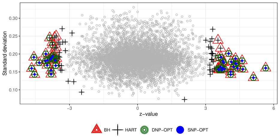
Figure 2: The scatter plot of $Z$ vs $\sigma$. The red triangles ($\triangle$) label the 51 discoveries by the BH procedure. The black plus ($+$) labels the 89 discoveries by HART. The green circle ($\bigcirc$) labels the 44 discoveries by DNP-OPT. The blue solid circle ($\bullet$) label the 37 discoveries by SNP-OPT. All the procedures target FDR level at 0.05.

We apply BH, HART as well as our SNP-OPT and DNP-OPT to the microarray data. All procedures target to control FDR at level 0.05. For SNP-OPT and DNP-OPT, we simply plug in the differential difference and the pooled standard deviation estimate to our procedures. For BH, we will use the $p$-values converted from the $z$-value as $p_{i}=2\Phi(-|z_{i}|)$ where $\Phi$ is the CDF of the standard normal distribution. HART estimates the sparsity level using Jin and Cai (2007) and provides an optional jackknifed procedure to estimate the marginal density.

BH and HART reject more hypotheses than SNP-OPT and DNP-OPT. Note that both BH and HART tend to be over-confident in the simulation. We cannot say much since the ground truth is unknown. However, we should focus on the shape of the rejection region. As in Figure 2, the rejection regions of DNP-OPT and SNP-OPT depend on both $z_{i}$ and $\sigma_{i}$ – hypotheses correspond to large $\sigma_{i}$ tend not to get rejected. We further compare with Storey’s procedure and a variant of HART and adjust the empirical null as suggested in Efron (2004) in the Appendix.

6 Summary and Discussion

In this paper, we propose a novel Spike-and-Nonparametric mixture prior (SNP) to tackle the high-dimensional sparse and heteroscedastic signal recovery problem. We develop an EM algorithm to estimate the unknown prior and derive the posterior. With the posterior, we are able to provide both point estimates with shrinkage/thresholding property and credible intervals for uncertainty quantification. In addition, our method estimates sparsity well, more accurate than the state-of-the-art methods. Based on our posterior, we also propose an optimal multiple testing procedure controlling FDR while achieving higher power.

So far we only discuss the independent settings. However, our method can be extended to correlated ${\mathbf{y}}$ using a two-stage procedure – we first estimate the prior ignoring correlations; and then we apply Markov chain Monte Carlo (MCMC) with Gibbs samplers to obtain the posterior.

Appendix A Appendix

Please find the Appendix in the supplemental material.

References

- Abadie and Kasy (2019) Alberto Abadie and Maximilian Kasy. Choosing among regularized estimators in empirical economics: The risk of machine learning. Review of Economics and Statistics, 101(5):743–762, 2019.
- Abraham et al. (2021) Kweku Abraham, Ismael Castillo, and Etienne Roquain. Empirical bayes cumulative multiple testing procedure for sparse sequences. arXiv preprint arXiv:2102.00929, 2021.
- Abramovich et al. (2006) F. Abramovich, Y. Benjamini, D. L. Donoho, and I. M. Johnstone. Adapting to Unknown Sparsity by Controlling the False Discovery Rate. The Annals of Statistics, 34(2):584–653, 2006.
- Azevedo et al. (2020) Eduardo M Azevedo, Alex Deng, José Luis Montiel Olea, Justin Rao, and E Glen Weyl. A/b testing with fat tails. Journal of Political Economy, 128(12):4614–000, 2020.
- Banerjee et al. (2021) Sayantan Banerjee, Ismaël Castillo, and Subhashis Ghosal. Bayesian inference in high-dimensional models. arXiv preprint arXiv:2101.04491, 2021.
- Banerjee et al. (2020) Trambak Banerjee, Luella Fu, Gareth M James, and Wenguang Sun. Nonparametric empirical bayes estimation on heterogeneous data. 2020.
- Belitser and Ghosal (2020) Eduard Belitser and Subhashis Ghosal. Empirical bayes oracle uncertainty quantification for regression. The Annals of Statistics, 48(6):3113–3137, 2020.
- Benjamini and Hochberg (1995) Yoav Benjamini and Yosef Hochberg. Controlling the false discovery rate: a practical and powerful approach to multiple testing. Journal of the Royal statistical society: series B (Methodological), 57(1):289–300, 1995.
- Benjamini et al. (2001) Yoav Benjamini, Daniel Yekutieli, et al. The control of the false discovery rate in multiple testing under dependency. The annals of statistics, 29(4):1165–1188, 2001.
- Benjamini et al. (2006) Yoav Benjamini, Abba M Krieger, and Daniel Yekutieli. Adaptive linear step-up procedures that control the false discovery rate. Biometrika, 93(3):491–507, 2006.
- Bogdan et al. (2011) Małgorzata Bogdan, Arijit Chakrabarti, Florian Frommlet, and Jayanta K Ghosh. Asymptotic bayes-optimality under sparsity of some multiple testing procedures. The Annals of Statistics, 39(3):1551–1579, 2011.
- Brown (2008) Lawrence D Brown. In-season prediction of batting averages: A field test of empirical bayes and bayes methodologies. The Annals of Applied Statistics, pages 113–152, 2008.
- Brown and Greenshtein (2009) Lawrence D Brown and Eitan Greenshtein. Nonparametric empirical bayes and compound decision approaches to estimation of a high-dimensional vector of normal means. The Annals of Statistics, pages 1685–1704, 2009.
- Cai et al. (2019) Junhui Cai, Avishai Mandelbaum, Chaitra H Nagaraja, Haipeng Shen, Linda Zhao, et al. Statistical theory powering data science. Statistical Science, 34(4):669–691, 2019.
- Carvalho et al. (2010) Carlos M Carvalho, Nicholas G Polson, and James G Scott. The horseshoe estimator for sparse signals. Biometrika, 97(2):465–480, 2010.
- Castillo and Roquain (2020) Ismaël Castillo and Étienne Roquain. On spike and slab empirical bayes multiple testing. The Annals of Statistics, 48(5):2548–2574, 2020.
- Castillo and Szabó (2020) Ismaël Castillo and Botond Szabó. Spike and slab empirical bayes sparse credible sets. Bernoulli, 26(1):127–158, 2020.
- Castillo and van der Vaart (2012) Ismaël Castillo and Aad van der Vaart. Needles and straw in a haystack: Posterior concentration for possibly sparse sequences. The Annals of Statistics, 40(4):2069–2101, 2012.
- Dabney et al. (2010) Alan Dabney, John D Storey, and GR Warnes. qvalue: Q-value estimation for false discovery rate control. R package version, 1(0), 2010.
- Dempster et al. (1977) Arthur P Dempster, Nan M Laird, and Donald B Rubin. Maximum likelihood from incomplete data via the em algorithm. Journal of the Royal Statistical Society: Series B (Methodological), 39(1):1–22, 1977.
- Efron (2004) Bradley Efron. Large-scale simultaneous hypothesis testing: the choice of a null hypothesis. Journal of the American Statistical Association, 99(465):96–104, 2004.
- Efron (2012) Bradley Efron. Large-scale inference: empirical Bayes methods for estimation, testing, and prediction, volume 1. Cambridge University Press, 2012.
- Efron (2014) Bradley Efron. Two modeling strategies for empirical bayes estimation. Statistical science: a review journal of the Institute of Mathematical Statistics, 29(2):285, 2014.
- Efron et al. (2001) Bradley Efron, Robert Tibshirani, John D Storey, and Virginia Tusher. Empirical bayes analysis of a microarray experiment. Journal of the American statistical association, 96(456):1151–1160, 2001.
- Efron et al. (2007) Bradley Efron et al. Size, power and false discovery rates. The Annals of Statistics, 35(4):1351–1377, 2007.
- Efron et al. (2019) Bradley Efron et al. Bayes, oracle bayes and empirical bayes. Statistical science, 34(2):177–201, 2019.
- Fu et al. (2020) Luella Fu, Bowen Gang, Gareth M James, and Wenguang Sun. Heteroscedasticity-adjusted ranking and thresholding for large-scale multiple testing. Journal of the American Statistical Association, pages 1–13, 2020.
- George and Foster (2000) E. I. George and D. P. Foster. Calibration and empirical Bayes variable selection. Biometrika, 87:731–747, 2000.
- George and McCulloch (1993) Edward I George and Robert E McCulloch. Variable selection via gibbs sampling. Journal of the American Statistical Association, 88(423):881–889, 1993.
- Goldberg and Johndrow (2017) David Goldberg and James E Johndrow. A decision theoretic approach to a/b testing. arXiv preprint arXiv:1710.03410, 2017.
- Guo et al. (2020) F Richard Guo, James McQueen, and Thomas S Richardson. Empirical bayes for large-scale randomized experiments: a spectral approach. arXiv preprint arXiv:2002.02564, 2020.
- Heckman and Singer (1984) James Heckman and Burton Singer. A method for minimizing the impact of distributional assumptions in econometric models for duration data. Econometrica: Journal of the Econometric Society, pages 271–320, 1984.
- Ignatiadis et al. (2016) Nikolaos Ignatiadis, Bernd Klaus, Judith B Zaugg, and Wolfgang Huber. Data-driven hypothesis weighting increases detection power in genome-scale multiple testing. Nature methods, 13(7):577–580, 2016.
- Ishwaran and Rao (2003) Hemant Ishwaran and J Sunil Rao. Detecting differentially expressed genes in microarrays using bayesian model selection. Journal of the American Statistical Association, 98(462):438–455, 2003.
- Ishwaran and Rao (2011) Hemant Ishwaran and J Sunil Rao. Consistency of spike and slab regression. Statistics & probability letters, 81(12):1920–1928, 2011.
- Ishwaran et al. (2005) Hemant Ishwaran, J Sunil Rao, et al. Spike and slab variable selection: frequentist and bayesian strategies. Annals of statistics, 33(2):730–773, 2005.
- James and Stein (1961) W. James and C. Stein. Estimation with quadratic loss. In Proc. 4th Berkeley Symp. Math. Statist. Prob., pages 361–379, 1961.
- Jiang and Zhang (2009) Wenhua Jiang and Cun-Hui Zhang. General maximum likelihood empirical bayes estimation of normal means. The Annals of Statistics, 37(4):1647–1684, 2009.
- Jiang and Zhang (2010) Wenhua Jiang and Cun-Hui Zhang. Empirical bayes in-season prediction of baseball batting averages. In Borrowing Strength: Theory Powering Applications–A Festschrift for Lawrence D. Brown, pages 263–273. Institute of Mathematical Statistics, 2010.
- Jiang et al. (2020) Wenhua Jiang et al. On general maximum likelihood empirical bayes estimation of heteroscedastic iid normal means. Electronic Journal of Statistics, 14(1):2272–2297, 2020.
- Jin and Cai (2007) Jiashun Jin and T Tony Cai. Estimating the null and the proportion of nonnull effects in large-scale multiple comparisons. Journal of the American Statistical Association, 102(478):495–506, 2007.
- Johnstone and Silverman (2004) I. M. Johnstone and B. W. Silverman. Needles and straw in haystacks: Empirical Bayes estimates of possibly sparse sequences. The Annals of Statistics, 32(4):1594–1649, 2004.
- Koenker and Gu (2017) Roger Koenker and Jiaying Gu. Rebayes: Empirical bayes mixture methods in r. Journal of Statistical Software, 82(8):1–26, 2017.
- Koenker and Mizera (2013) Roger Koenker and Ivan Mizera. Convex optimization, shape constraints, compound decisions, and empirical bayes rules. Journal of the American Statistical Association, 2013.
- Laird (1978) Nan Laird. Nonparametric maximum likelihood estimation of a mixing distribution. Journal of the American Statistical Association, 73(364):805–811, 1978.
- Lei and Fithian (2016) Lihua Lei and William Fithian. Adapt: an interactive procedure for multiple testing with side information. arXiv preprint arXiv:1609.06035, 2016.
- Leng et al. (2013) Ning Leng, John A Dawson, James A Thomson, Victor Ruotti, Anna I Rissman, Bart MG Smits, Jill D Haag, Michael N Gould, Ron M Stewart, and Christina Kendziorski. Ebseq: an empirical bayes hierarchical model for inference in rna-seq experiments. Bioinformatics, 29(8):1035–1043, 2013.
- Liao et al. (2020) Peng Liao, Kristjan Greenewald, Predrag Klasnja, and Susan Murphy. Personalized heartsteps: A reinforcement learning algorithm for optimizing physical activity. Proceedings of the ACM on Interactive, Mobile, Wearable and Ubiquitous Technologies, 4(1):1–22, 2020.
- Park and Casella (2008) Trevor Park and George Casella. The bayesian lasso. Journal of the American Statistical Association, 103(482):681–686, 2008.
- Perone Pacifico et al. (2004) Marco Perone Pacifico, Christopher Genovese, Isabella Verdinelli, and Larry Wasserman. False discovery control for random fields. Journal of the American Statistical Association, 99(468):1002–1014, 2004.
- Raykar and Zhao (2010) Vikas C Raykar and Linda H Zhao. Nonparametric prior for adaptive sparsity. In International Conference on Artificial Intelligence and Statistics, pages 629–636, 2010.
- Robbins (1956) Herbert Robbins. A sequential decision problem with a finite memory. Proceedings of the National Academy of Sciences of the United States of America, 42(12):920, 1956.
- Rocková (2018) Veronika Rocková. Bayesian estimation of sparse signals with a continuous spike-and-slab prior. The Annals of Statistics, 46(1):401–437, 2018.
- Rockova and George (2016) Veronika Rockova and Edward I George. The spike-and-slab lasso. Journal of the American Statistical Association, (just-accepted), 2016.
- Rousseau and Szabo (2020) Judith Rousseau and Botond Szabo. Asymptotic frequentist coverage properties of bayesian credible sets for sieve priors. The Annals of Statistics, 48(4):2155–2179, 2020.
- Sarkar et al. (2008) Sanat K Sarkar, Tianhui Zhou, and Debashis Ghosh. A general decision theoretic formulation of procedures controlling fdr and fnr from a bayesian perspective. Statist. Sinica, 18(3):925–945, 2008.
- Schwartzman et al. (2008) Armin Schwartzman, Robert F Dougherty, Jonathan E Taylor, et al. False discovery rate analysis of brain diffusion direction maps. Annals of Applied Statistics, 2(1):153–175, 2008.
- Singh et al. (2002) Dinesh Singh, Phillip G Febbo, Kenneth Ross, Donald G Jackson, Judith Manola, Christine Ladd, Pablo Tamayo, Andrew A Renshaw, Anthony V D’Amico, Jerome P Richie, et al. Gene expression correlates of clinical prostate cancer behavior. Cancer cell, 1(2):203–209, 2002.
- Stephens (2017) Matthew Stephens. False discovery rates: a new deal. Biostatistics, 18(2):275–294, 2017.
- Storey (2002) John D Storey. A direct approach to false discovery rates. Journal of the Royal Statistical Society: Series B (Statistical Methodology), 64(3):479–498, 2002.
- Storey et al. (2003) John D Storey et al. The positive false discovery rate: a bayesian interpretation and the q-value. The Annals of Statistics, 31(6):2013–2035, 2003.
- Su et al. (2016) Weijie Su, Emmanuel Candes, et al. Slope is adaptive to unknown sparsity and asymptotically minimax. Annals of Statistics, 44(3):1038–1068, 2016.
- Sun and Cai (2007) Wenguang Sun and T Tony Cai. Oracle and adaptive compound decision rules for false discovery rate control. Journal of the American Statistical Association, 102(479):901–912, 2007.
- Tang and Zhang (2007) Weihua Tang and Cun-Hui Zhang. Empirical bayes methods for controlling the false discovery rate with dependent data. Complex Datasets and Inverse Problems, pages 151–160, 2007.
- Tibshirani (1996) Robert Tibshirani. Regression shrinkage and selection via the lasso. Journal of the Royal Statistical Society: Series B (Methodological), 58(1):267–288, 1996.
- van der Pas et al. (2017) Stéphanie van der Pas, Botond Szabó, and Aad van der Vaart. Uncertainty quantification for the horseshoe (with discussion). Bayesian Analysis, 12(4):1221–1274, 2017.
- Wand and Jones (1994) Matt P Wand and M Chris Jones. Kernel smoothing. Crc Press, 1994.
- Weinstein et al. (2018) Asaf Weinstein, Zhuang Ma, Lawrence D Brown, and Cun-Hui Zhang. Group-linear empirical bayes estimates for a heteroscedastic normal mean. Journal of the American Statistical Association, 113(522):698–710, 2018.
- Woody and Scott (2018) Spencer Woody and James G Scott. Optimal post-selection inference for sparse signals: a nonparametric empirical-bayes approach. arXiv preprint arXiv:1810.11042, 2018.
- Xie et al. (2012) Xianchao Xie, SC Kou, and Lawrence D Brown. Sure estimates for a heteroscedastic hierarchical model. Journal of the American Statistical Association, 107(500):1465–1479, 2012.
- Yekutieli (2012) Daniel Yekutieli. Adjusted bayesian inference for selected parameters. Journal of the Royal Statistical Society: Series B (Statistical Methodology), 74(3):515–541, 2012.
- Yu and Hoff (2018) Chaoyu Yu and Peter D Hoff. Adaptive multigroup confidence intervals with constant coverage. Biometrika, 105(2):319–335, 2018.