Covariance-based smoothed particle hydrodynamics. A machine-learning application to simulating disc fragmentation

Abstract

A PCA-based, machine learning version of the SPH method is proposed. In the present scheme, the smoothing tensor is computed to have their eigenvalues proportional to the covariance’s principal components, using a modified octree data structure, which allows the fast estimation of the anisotropic self-regulating kNN. Each SPH particle is the center of such an optimal kNN cluster, i.e., the one whose covariance tensor allows the find of the kNN cluster itself according to the Mahalanobis metric. Such machine learning constitutes a fixed point problem. The definitive (self-regulating) kNN cluster defines the smoothing volume, or properly saying, the smoothing ellipsoid, required to perform the anisotropic interpolation. Thus, the smoothing kernel has an ellipsoidal profile, which changes how the kernel gradients are computed. As an application it was performed the simulation of collapse and fragmentation of a non-magnetic, rotating gaseous sphere. An interesting outcome was the formation of protostars in the disc fragmentation, shown to be much more persistent and much more abundant in the anisotropic simulation than in the isotropic case.

1 Introduction

The present work consists of combining machine learning with the numerical methods of smoothed particle hydrodynamics (SPH). The machine learning approach is used to find the optimal smoothing volumes that best express the anisotropic tendencies of the particle distribution, as previously proposed by Marinho [2014]. These ideal volumes are defined in terms of the self-regulating kNN clusters, as will be seen later.

SPH is a Lagrangian computational method of fluid mechanics that was introduced by two independent works [Gingold and Monaghan, 1977, Lucy, 1977]. On the other hand, machine learning consists of an algorithm, or a combination of algorithms, that automatically refines the approximate solution to a pattern recognition problem, allowing future classifications to be more efficient once the machine has acquired experience from the previous classification [Duda et al., 2001].

One of the main problems of SPH concerns the best morphology of the smoothing volume, regarding the optimal spatial resolution. A first attempt to improve spatial resolution is to consider each simulation particle (say, query particle) as the center of its $k$-nearest neighbors [e.g. Monaghan, 1992, 1994, 2012], which in turn is a variant of the Parzen window [e.g. Duda et al., 2001]. In such estimation technique the smoothing kernel is spherical, with smoothing length proportional to $\rho^{-1/3}$. Therefore, the orthodox adaptive SPH is in fact a density-adaptive scheme, which in principle disregard the multivariate distribution of the simulation particles.

A second advance made in order to obtain a more complete spatial adaptability, both in density and in the preferential direction of deformation of the smoothing volume, was proposed by [Martel et al., 1993, hereafter MSVK], which named the adaptive technique as ASPH, followed by the works of Shapiro et al. [1996], Owen et al. [1998] and Martel and Shapiro [2003]. The authors introduced a tensor version of the smoothing length, namely, the smoothing tensor $\mathbf{H}$, whose components change in space and time according to the estimated deformation-rate tensor, $\bm{\nabla}\bm{v}$. The squared smoothing tensor $\mathbf{H}^{2}$ is the metric tensor whose minimal surface of equidistant points containing all the kNN corresponds to the ellipsoid whose semi-major axes are the eigenvalues (eigenvectors) of $\mathbf{H}$.

In the present work, a machine learning technique is proposed, which in a way resembles the MSVK technique, but is based on the principal components analysis (PCA), using the anisotropic search method for the $k$-nearest neighbors ($k$-NN) proposed by Marinho and Andreazza [2010]. The Marinho–Andreazza approach is an unsupervised machine learning method of finding the optimal $k$-NN set, under the Mahalanobis metric [Mahalanobis, 1936], named here as the self-regulating $k$-NN cluster. The proposed anisotropic SPH code is a covariance-based SPH, addressed hereafter as Sigma-SPH.

What is new in this work is that the anisotropic kernel is defined only by multivariate arguments, involving the properties of the covariance tensor, without taking into account the ASPH technique. In summary, Sigma-SPH is based solely on the multivariability of the particle distribution, while in ASPH the smoothing tensor is defined according to the dynamics of the simulated fluid, via deformation rate tensor.

Presently, the smoothing tensor is proportional to the squared root of the covariance tensor, namely $\mathbf{H}=\gamma_{\mathrm{max}}\mathbf{\Sigma}^{1/2}$, where $\gamma_{\mathrm{max}}$ is the Mahalanobis distance from the query particle to the outermost one in the self-regulating $k$-NN cluster. Thus, $\mathbf{H}$ is the tensor whose eigenvalues/eigenvectors sets up the minimal ellipsoid hull of the self-regulating $k$-NN cluster.

To continue, we will use pattern recognition terminology, such as the dataset concept, adapted for the set of particles used in the SPH simulation. An SPH dataset is seen as a collection of classic $N$ particles, seen as massive points in the configuration space. Each particle has then three coordinates for positions and three coordinates for velocities. It is assumed that the particles are distinguishable only by their positions, regardless of their other physical attributes. The coordinates of the particles make up a unique query key. Further relevant quantities are attributed to the particles in the dataset, such as specific thermal energy. Of course, each particle is represented by an instance in the dataset.

In the present work, we are concerned with the three-dimensional description of SPH particles in euclidean space $\mathbb{E}^{3}$ so that velocities and other intrinsic quantities are field functions of spatial coordinates. Time is naturally implicit in the Lagrangian equations of fluid motion.

For simplicity and mathematical conciseness, we abstract the dataset as a collection of identifiers or indexes, which form a bijection with the spatial coordinates of the particles. Thus, we refer to the dataset as simply the index collection $\mathcal{D}=\{1,2,\ldots,N\}$ whenever necessary. Any subset $\mathcal{C}$ of $\mathcal{D}$ is called a cluster. In particular, we are primarily interested in clusters that constitute a partition of $\mathcal{D}$. For instance, $\mathcal{A}$ and $\mathcal{B}$ constitute a cluster partition if and only if $\mathcal{A}\cup\mathcal{B}=\mathcal{D}$ and $\mathcal{A}\cap\mathcal{B}=\emptyset$.

If $\mathcal{C}$ is a cluster within $\mathcal{D}$, we assume the following correspondence:

$$\mathcal{C}=\{i_{1},i_{2},\ldots,i_{k}\}\subseteq\{1,\ldots,N\}$$ (1)

Thus, the cluster’s total mass is written as

$$M_{\mathcal{C}}=\sum_{j\in\mathcal{C}}m_{j}$$ (2)

The cluster’s center of mass, aka cluster’s mean position, is written as the following normalized first momentum:

$$\bm{r}_{\mathcal{C}}=\frac{1}{M_{\mathcal{C}}}\sum_{j\in\mathcal{C}}m_{j}\bm{r}_{j}$$ (3)

The cluster’s covariance tensor [e.g. Duda et al., 2001] is defined as

$$\mathbf{\Sigma}_{\mathcal{C}}=\frac{1}{M_{\mathcal{C}}}\sum_{j\in\mathcal{C}}m_{j}(\bm{r}_{j}-\bm{r}_{\mathcal{C}})\otimes(\bm{r}_{j}-\bm{r}_{\mathcal{C}})$$ (4)

$\otimes$ stands for the tensor product, defined here as the outer product $\otimes:\mathbb{E}^{3}\times\mathbb{E}^{3}\mapsto\mathbb{E}^{3^{2}}$, which in matrix notation corresponds to

$$\bm{A}\otimes\bm{B}\equiv\bm{A}\bm{B}^{t}$$ (5)

where

$$\bm{A}\equiv\begin{pmatrix}A_{1}\\ A_{2}\\ A_{3}\end{pmatrix}\in\mathbb{R}^{3}\;\text{and}\;\bm{B}^{t}\equiv\begin{pmatrix}B_{1}B_{2}B_{3}\end{pmatrix}\in(\mathbb{R}^{3})^{t}$$ (6)

and $(\mathbb{R}^{3})^{t}$ is the dual space of $\mathbb{R}^{3}$. Thus, from equation (5),

$$\bm{A}\otimes\bm{B}\equiv\bm{A}\bm{B}^{t}\equiv\begin{pmatrix}A_{1}B_{1}&A_{1}B_{2}&A_{1}B_{3}\\ A_{2}B_{1}&A_{2}B_{2}&A_{2}B_{3}\\ A_{3}B_{1}&A_{3}B_{2}&A_{3}B_{3}\end{pmatrix}\in\mathbb{R}^{3}\otimes\mathbb{R}^{3}$$ (7)

where the tensor-product space, $\mathbb{R}^{3}\otimes\mathbb{R}^{3}$, is isomorphic to the vector space of the real $3\times 3$ square matrices, namely $\mathbb{R}^{3}\otimes\mathbb{R}^{3}\equiv\mathbb{R}^{3^{2}}$.

On the other hand, the scalar product $\bm{A}\cdot\bm{B}$ has its matrix representation given by

$$\bm{A}\cdot\bm{B}\equiv\bm{A}^{t}\bm{B}$$ (8)

It follows immediately from the definitions for $\bm{A}$ and $\bm{B}$, previously given in equation (6), that

$$\bm{A}\cdot\bm{B}\equiv\bm{A}^{t}\bm{B}\equiv A_{1}B_{1}+A_{2}B_{2}+A_{3}B_{3}=\text{tr\ }\bm{A}\bm{B}^{t}$$ (9)

where $\text{tr\ }\bm{A}{\bm{B}}^{t}$ is the trace of the matrix $\bm{A}{\bm{B}}^{t}$ according to equations (5) and (7)

For notation brevity, and regarding equation (5), the covariance tensor can be written simply as

$$\mathbf{\Sigma}_{\mathcal{C}}=\frac{1}{M_{\mathcal{C}}}\sum_{j\in\mathcal{C}}m_{j}(\bm{r}_{j}-\bm{r}_{\mathcal{C}})(\bm{r}_{j}-\bm{r}_{\mathcal{C}})^{t}$$ (10)

The cluster’s variance $\sigma_{\mathcal{C}}^{2}$ is computed as

$${\sigma}_{\mathcal{C}}^{2}=\frac{1}{M_{\mathcal{C}}}\sum_{j\in\mathcal{C}}m_{j}(\bm{r}_{j}-\bm{r}_{\mathcal{C}})^{t}(\bm{r}_{j}-\bm{r}_{\mathcal{C}})\equiv\text{tr\ }\mathbf{\Sigma}_{\mathcal{C}}$$ (11)

which is the isotropic measure of the cluster’s dispersion, in contrast to the fact that $\mathbf{\Sigma}_{\mathcal{C}}$ measures the anisotropic data dispersion. The latter result, ${\sigma}_{\mathcal{C}}^{2}\equiv\text{tr\ }\mathbf{\Sigma}_{\mathcal{C}},$ comes from equation (9).

Since $\mathbf{\Sigma}_{\mathcal{C}}$ is positive definite, it comes immediately that

$$\text{tr\ }\mathbf{\Sigma}_{\mathcal{C}}>0.$$

The ${\sigma}_{\mathcal{C}}^{2}=0$ case is not considered since the entire dataset $\mathcal{D}$ would degenerate into a single particle.

One cautionary remark is that the number of non-zero eigenvalues of the tensor $\mathbf{\Sigma}_{\mathcal{C}}$ depends on the distribution topology. For instance, if the entire dataset degenerates into a plane surface, it means that there is one null eigenvalue. Such a situation is almost improbable in a 3D SPH simulation due to the initial conditions’ randomization or, maybe, to the 3D crystalline initial configuration, combined with the freedom of motion an SPH particle has; see, for instance, the later section on the SPH equations of motion. A difficulty can happen in situations of strong compressive shocks, which can reduce the shock thickness to almost zero. In this case, some tolerance artifice must be used to prevent singularities.

The vector collection

$$\bm{p}=\{\sigma_{1}\bm{e}_{1},\;\sigma_{2}\bm{e}_{2},\;\sigma_{3}\bm{e}_{3}\}$$ (12)

is named the principal components of the covariance tensor $\mathbf{\Sigma}_{\mathcal{C}}$, whereas the ordered set

$$\bm{\sigma}=\{\sigma_{1}^{2},\,\sigma_{2}^{2},\,\sigma_{3}^{2}\;|\;\sigma_{1}\leq\sigma_{2}\leq\sigma_{3}\}$$ (13)

is the collection of eigenvalues of $\mathbf{\Sigma}_{\mathcal{C}}$. The collection $\{\bm{e}_{1},\bm{e}_{2},\bm{e}_{3}\}$ of unit vectors corresponds to the normalized eigenvectors of the tensor $\mathbf{\Sigma}_{\mathcal{C}}$. Consequently, the diagonal representation of the covariance tensor, adopting the convention (5), is given by

$$\mathbf{\Sigma}_{\mathcal{C}}=\sigma_{1}^{2}\,\bm{e}_{1}\bm{e}_{1}^{t}+\sigma_{2}^{2}\,\bm{e}_{2}\bm{e}_{2}^{t}+\sigma_{3}^{2}\,\bm{e}_{3}\bm{e}_{3}^{t}$$ (14)

It follows straightforwardly that the diagonal form of the inverse covariance tensor can be written as in an analogous form of equation (14):

$$\mathbf{\Sigma}_{\mathcal{C}}^{-1}=\frac{1}{\sigma_{1}^{2}}\,\bm{e}_{1}\bm{e}_{1}^{t}+\frac{1}{\sigma_{2}^{2}}\,\bm{e}_{2}\bm{e}_{2}^{t}+\frac{1}{\sigma_{3}^{2}}\,\bm{e}_{3}\bm{e}_{3}^{t}$$ (15)

The Mahalanobis distance, which is a measure of how a data point varies toward different directions about the mean cluster position, $\bm{r}_{\mathcal{C}}$, is defined as

$$\delta^{2}=(\bm{r}-\bm{r}_{\mathcal{C}})\cdot\mathbf{\Sigma}_{\mathcal{C}}^{-1}\cdot(\bm{r}-\bm{r}_{\mathcal{C}})\equiv(\bm{r}-\bm{r}_{\mathcal{C}})^{t}\mathbf{\Sigma}_{\mathcal{C}}^{-1}(\bm{r}-\bm{r}_{\mathcal{C}})$$ (16)

Observing equation (15), and assuming that the eigenvalues and eigenvectors are both known, we have a very simplified form of the latter equation:

$$\delta^{2}=\biggl{[}\frac{(\bm{r}-\bm{r}_{\mathcal{C}})\cdot\bm{e}_{1}}{\sigma_{1}}\biggr{]}^{2}+\biggl{[}\frac{(\bm{r}-\bm{r}_{\mathcal{C}})\cdot\bm{e}_{2}}{\sigma_{2}}\biggr{]}^{2}+\biggl{[}\frac{(\bm{r}-\bm{r}_{\mathcal{C}})\cdot\bm{e}_{3}}{\sigma_{3}}\biggr{]}^{2}$$ (17)

The collection of points in $\mathbb{E}^{3}$ whose Mahalanobis distance $\delta(\bm{r})$ to the origin equals the unit is defined as the confidence ellipsoid, namely,

$$\mathcal{E}_{\mathcal{C}}^{3}=\{\bm{r}\in\mathbb{E}^{3}|\delta(\bm{r})=1\}$$ (18)

which is equivalent to the solution for the equation

$$\biggl{[}\frac{(\bm{r}-\bm{r}_{\mathcal{C}})\cdot\bm{e}_{1}}{\sigma_{1}}\biggr{]}^{2}+\biggl{[}\frac{(\bm{r}-\bm{r}_{\mathcal{C}})\cdot\bm{e}_{2}}{\sigma_{2}}\biggr{]}^{2}+\biggl{[}\frac{(\bm{r}-\bm{r}_{\mathcal{C}})\cdot\bm{e}_{3}}{\sigma_{3}}\biggr{]}^{2}=1$$ (19)

Particularly, doing the following transform

$$\xi_{1}=\frac{(\bm{r}-\bm{r}_{\mathcal{C}})\cdot\bm{e}_{1}}{\sigma_{1}},\;\xi_{2}=\frac{(\bm{r}-\bm{r}_{\mathcal{C}})\cdot\bm{e}_{2}}{\sigma_{2}},\;\xi_{3}=\frac{(\bm{r}-\bm{r}_{\mathcal{C}})\cdot\bm{e}_{3}}{\sigma_{3}},$$ (20)

we have

$$\xi_{1}^{2}+\xi_{2}^{2}+\xi_{3}^{2}=1,$$ (21)

which is the equation of a unit sphere $\mathcal{S}_{1}$ in the uncorrelated vector space

$$\mathbb{U}^{3}_{\mathcal{C}}=\{\bm{\xi}\;|\;\;\bm{\xi}=\mathbf{\Sigma}_{\mathcal{C}}^{-1/2}(\bm{r}-\bm{r}_{\mathcal{C}})\}$$ (22)

whose position vector $\bm{\xi}$ have coordinates $(\xi_{1},\xi_{2},\xi_{3})$. Such a vector space, spanning at the average cluster’s position $\bm{r}_{\mathcal{C}},$ in which the Mahalanobis metric is transformed into the euclidean one, is named the uncorrelated vector space. Thus, it is given any vector $\bm{r}\in\mathbb{E}^{3}$ an uncorrelated vector $\bm{\xi}\in\mathbb{U}^{3}_{\mathcal{C}}$, once known the mean position $\bm{r}_{\mathcal{C}}$, according to the normalization given in (20), namely

$$\bm{\xi}=\xi_{1}\bm{e}_{1}+\xi_{2}\bm{e}_{2}+\xi_{3}\bm{e}_{3}$$ (23)

It has been used in equation (22) the square root of the covariance tensor in its diagonal form, namely,

$$\mathbf{\Sigma}_{\mathcal{C}}^{1/2}\equiv\sigma_{1}\bm{e}_{1}\bm{e}_{1}^{t}+\sigma_{2}\bm{e}_{2}\bm{e}_{2}^{t}+\sigma_{3}\bm{e}_{3}\bm{e}_{3}^{t},$$ (24)

whose inverse $\mathbf{\Sigma}_{\mathcal{C}}^{-1/2}$ can be easily computed as

$$\mathbf{\Sigma}_{\mathcal{C}}^{-1/2}\equiv\frac{\bm{e}_{1}\bm{e}_{1}^{t}}{\sigma_{1}}+\frac{\bm{e}_{2}\bm{e}_{2}^{t}}{\sigma_{2}}+\frac{\bm{e}_{3}\bm{e}_{3}^{t}}{\sigma_{3}}.$$ (25)

One shall notice that the square module of $\bm{\xi}\in\mathbb{U}^{3}_{\mathcal{C}}$ is computed accordingly to the following dot-product:

$$|\bm{\xi}|^{2}=\mathbf{\Sigma}_{\mathcal{C}}^{-1/2}(\bm{r}-\bm{r}_{\mathcal{C}})\cdot\mathbf{\Sigma}_{\mathcal{C}}^{-1/2}(\bm{r}-\bm{r}_{\mathcal{C}})\equiv(\bm{r}-\bm{r}_{\mathcal{C}})^{t}\mathbf{\Sigma}_{\mathcal{C}}^{-1}(\bm{r}-\bm{r}_{\mathcal{C}}),$$ (26)

which turns back to the Mahalanobis distance from $\bm{r}$ to the mean $\bm{r}_{\mathcal{C}}$ under the covariance tensor $\mathbf{\Sigma}_{\mathcal{C}}$. On the other hand, one finds from equations (20) and (23) that

$$|\bm{\xi}|=\sqrt{\xi_{1}^{2}+\xi_{2}^{2}+\xi_{3}^{2}}$$ (27)

is the euclidean distance from $\bm{\xi}$ to the origin of the uncorrelated space $\mathbb{U}^{3}_{\mathcal{C}}$. Thus, equation (21) connects the confidence ellipsoid $\mathcal{E}_{\mathcal{C}}^{3}$ in $\mathbb{E}^{3}$ with the unit sphere $\mathcal{S}_{\mathcal{C}}^{3}=\{\bm{\xi}\in\mathbb{U}^{3}_{\mathcal{C}}\;|\;\;|\bm{\xi}|=1\}.$

The original space $\mathbb{E}^{3}$ from which the dataset points have their spatial coordinates is called hereafter the correlated space once their points are correlated according to the covariance tensor. Thus, from the equation (22), we have the affine correlated vector space

$$\mathbb{E}^{3}=\{\bm{r}\;|\;\bm{r}=\mathbf{\Sigma}_{\mathcal{C}}^{1/2}\bm{\xi}+\bm{r}_{\mathcal{C}}\}.$$ (28)

transformed

We can generalize the Mahalanobis distance so that it is no longer restricted to its statistical meaning. Thus, if $\bm{a}$ and $\bm{b}$ are vectors in $\mathbb{E}^{3}$, their quadratic Mahalanobis distance is defined as follows

$$\delta^{2}(\bm{a},\bm{b})=(\bm{a}-\bm{b})\cdot\mathbf{\Sigma}_{\mathcal{C}}^{-1}\cdot(\bm{a}-\bm{b})$$

$$\equiv(\bm{a}-\bm{b})^{t}\mathbf{\Sigma}_{\mathcal{C}}^{-1}(\bm{a}-\bm{b}).$$ (29)

Transforming both $\bm{a}$ and $\bm{b}$ of $\mathbb{E}^{3}$ into the vectors $\bm{\xi}_{a}$ and $\bm{\xi}_{b}$ of the $\mathbb{U}^{3}_{\mathcal{C}}$ by means of definition (22), respectively, one can easily see that equation (29) is equivalent to the euclidean distance in $\mathbb{U}^{3}_{\mathcal{C}}$:

$$\delta^{2}(\bm{a},\bm{b})\equiv|\bm{\xi}_{a}-\bm{\xi}_{b}|^{2}$$ (30)

Moreover, replacing $\mathbf{\Sigma}_{\mathcal{C}}$ in equation (29) with the identity tensor $\mathbf{1}$, we have the quadratic form of the euclidean distance, namely,

$$\delta^{2}(\bm{a},\bm{b})=(\bm{a}-\bm{b})\cdot\mathbf{1}\cdot(\bm{a}-\bm{b})=|\bm{a}-\bm{b}|^{2}.$$ (31)

The latter result will be useful in initializing the recursive self-regulating kNN.

The purpose of the present work is to present and validate a computer program based on machine learning to perform fully adaptive SPH simulations, i.e., adaptive to the anisotropic nature of mass distribution in critical situations of shock and filamentary fragmentation. The paper is structured as follows.

In Sec. 2 is discussed the self-regulating kNN cluster machine learning approach. In Sec. 3 it is shown how to estimate the ellipsoidal hull for the self-regulating kNN cluster and consequently computing the smoothing tensor. The anisotropic model for the smoothing kernel is proposed in Sec. 4. The anisotropic smoothed particle hydrodynamics are discussed in Sec. 5. The anisotropic artificial viscosity model is proposed in Sec. 6. A brief description of the covariance-octree based gravity estimation as a modification to the Barnes and Hut [1986] method is made in Sec. 7. The adaptive multiple time-scale leapfrog is discussed in Sec. 8. As an application, it was performed a simulation of the collapse of a rotating gas sphere, which converges to a protostellar like disc, which will be discussed in details in Sec. 9. Discussion and conclusion are made in Sec. 10.

2 Self-regulating kNN cluster

This section presents a machine learning approach to find the anisotropic self-regulating kNN. The term self-regulating comes from the fact that the covariance tensor estimated over such an ideal cluster is the same tensor used to search back for the same kNN cluster according to the Mahalanobis metric. Thus, the method is a kind of fixed-point problem. If the learned k-NN cluster is reorganized so that its particles displace by a small amount, then the computational effort to find the new self-regulating cluster is small compared to the initial training. So we say that the method learns how the particles are distributed in a multivariate way.

The anisotropic kNN method is an approach for searching for the k-nearest neighbors of a query point accordingly to some tensor metric, introduced by Marinho and Andreazza [2010]. However, in that paper, the authors focused more on the proposed data structure: the covariance (hyper) quadtree, which allows the automatic reduction of dimensionality, proper of the PCA technique. This definition of anisotropic kNN is being rescued here in the form of an application to effectively determine the smoothing kernel’s compact support, which will be adopted later in the presently proposed anisotropic SPH. As the current purpose is to perform three-dimensional simulations, we renamed the data structure of Marinho–Andreazza as the covariance octree instead of the covariance quadtree. The self-regulating kNN cluster method is depicted as follows.

It is presumed that we already have an anisotropic kNN function as the method prescribed by Marinho and Andreazza [2010], namely,

$$\mathcal{N}(q_{0})=\{q_{0},q_{1},\ldots,q_{k}\},$$ (32)

given the index $q_{0}$ of the query particle located at position $\bm{r_{q_{0}}}$, and a predicted covariance tensor $\mathbf{\Sigma}$ to perform the search according to the Mahalanobis metric.

The positive closure $\mathcal{N}^{+}$ of the anisotropic kNN is given buy the subset $\mathcal{N}^{+}(q_{0})=\mathcal{N}(q_{0})-\{q_{0}\}=\{q_{1},\ldots,q_{k}\}$, which is the index set of the first $k$ nearest proper neighbors from $q_{0}$. Moreover, $\mathcal{N}(q_{0})$ is ordered by Mahalanobis distances, namely, $\delta(\bm{r}_{q_{1}},\bm{r}_{q_{0}})\leq\delta(\bm{r}_{q_{2}},\bm{r}_{q_{0}})\leq\cdots\leq\delta(\bm{r}_{q_{k}},\bm{r}_{q_{0}})$. If the particles are randomly distributed, the equality would very difficultly occur. Of course, $\delta(\bm{r}_{q_{0}},\bm{r}_{q_{0}})=0$ is a trivial result, and, in this case, $q_{0}$ is called an improper neighbor to itself. On the other hand, if $\delta(\bm{r}_{p},\bm{r}_{q})\neq 0$, then $p$ is said to be a proper neighbor of $q$. The set $\mathcal{N}(q_{0})$ of the anisotropic kNN constitutes the set of training points for the proposed machine learning method.

The initial step of the first training is made by using the identity tensor $\mathbf{1}$ in place of the predicted covariance tensor $\mathbf{\Sigma}$. By first training we mean the start approach in the beginning of the SPH simulation, before performing the integration scheme. Of course, such initialization switches the distance from anisotropic to euclidean. Thus, it gets the first attempt $\mathcal{C}^{(1)}_{k}\equiv\mathcal{N}(q_{0}|\mathbf{1})=\{q_{0},q_{1},\ldots,q_{k}\}$, which is of course isotropic. Thus, the $\mathcal{C}^{(1)}_{k}$ morphology is almost spherical if it is within $\mathcal{D}$ and far from its borders.

The next approach consists of iteratively computing the covariance tensor for the newly found anisotropic neighborhood to predict a neighborhood closer to the objective that is the self-regulating kNN cluster. Thus, as it has been computed $\mathcal{C}^{(n)}_{k}$ at iteration $n$, compute the covariance tensor $\mathbf{\Sigma}_{\mathcal{C}_{k}}^{(n)}$ for the newly found kNN cluster, and then estimate an ever more refined kNN list, namely

$$\mathcal{C}^{(n+1)}_{k}\leftarrow\mathcal{N}(q_{0}|\mathbf{\Sigma}_{\mathcal{C}_{k}}^{(n)}).$$ (33)

To recall, the covariance tensor is computed accordingly to equation (10) as follows

$$\mathbf{\Sigma}_{\mathcal{C}_{k}}=\frac{1}{M_{\mathcal{C}_{k}}}\sum_{j\in\mathcal{C}_{k}}m_{j}(\bm{r}_{j}-\bm{r}_{\mathcal{C}_{k}})(\bm{r}_{j}-\bm{r}_{\mathcal{C}_{k}})^{t}$$ (34)

where $\mathcal{C}_{k}$ is the anisotropic kNN cluster, having center of mass $\bm{r}_{\mathcal{C}_{k}}$. The quantities $M_{\mathcal{C}_{k}}$ and $\bm{r}_{\mathcal{C}_{k}}$ are computed from equations (2) and (3), respectively.

In order to perform the anisotropic kNN search, it is necessary to first estimate the eigenvalues/eigenvectors of the predicted $\mathbf{\Sigma}_{\mathcal{C}_{k}}$ to have the right-hand side of equation (25). It was presently adopted the power-iteration method to find a good approximation for eigenvalues. The method usually takes less than 10 steps to estimate both the eigenvalues and eigenvectors, and a similar count takes to have convergence to the self-regulating kNN per query. The power iteration method in the present code is just a heritage of the former code to perform cluster analysis and PCA in higher dimension spaces [e.g., Marinho and Andreazza, 2010].

According to the steps described above, it can be seen that as the method approaches convergence, a central part of the kNN cluster remains unchanged, leaving only a tenuous outer margin that is not yet conclusive. Certainly, this small population corresponds to particles outside the confidence ellipsoid. This residual population has only a few particles compared to the predefined number of nearest neighbors, presumably large enough, say, $k\gg 1$. However, this reasoning only works if the kNN cluster is far enough from the edges of the distribution.

Consistent with what was said in the previous paragraph, since the central part of the outgoing kNN cluster remains unchanged, it is immediate that the query’s position is increasingly closer to the center of mass of the kNN cluster. The empirical results show that convergence occurs, and the self-regulating kNN cluster has its center of mass located very approximates to the query position.

From equations (32) and (34), we find

$$\mathbf{\Sigma}_{\mathcal{C}_{k}}=\frac{1}{M_{\mathcal{C}_{k}}}\sum_{j=1}^{k}m_{q_{j}}(\bm{r}_{q_{j}}-\bm{r}_{\mathcal{C}_{k}})(\bm{r}_{q_{j}}-\bm{r}_{\mathcal{C}_{k}})^{t}+\Delta\mathbf{\Sigma}_{\mathcal{C}_{k}}$$ (35)

where the residual covariance tensor is written as

$$\Delta\mathbf{\Sigma}_{\mathcal{C}_{k}}=\frac{m_{q_{0}}}{M_{\mathcal{C}_{k}}}(\bm{r}_{q_{0}}-\bm{r}_{\mathcal{C}_{k}})(\bm{r}_{q_{0}}-\bm{r}_{\mathcal{C}_{k}})^{t}$$ (36)

In the stable configuration, when the residual covariance tensor goes to zero, $\Delta\mathbf{\Sigma}_{\mathcal{C}_{k}}\to\mathbf{0}$, as the query position approaches the cluster’s center of mass, $\bm{r}_{q_{0}}\to\bm{r}_{\mathcal{C}_{k}}$, the output kNN cluster becomes self-regulating, and then we have the following pair of self-consistent equations:

$$\mathbf{\Sigma}_{\mathcal{C}_{k}^{\text{sr}}}=\frac{1}{M_{\mathcal{C}_{k}^{\text{sr}}}}\sum_{j=1}^{k}m_{q_{j}}(\bm{r}_{q_{j}}-\bm{r}_{q_{0}})(\bm{r}_{q_{j}}-\bm{r}_{q_{0}})^{t},$$ (37)

and

$$\mathcal{C}_{k}^{\text{sr}}=\mathcal{N}(q_{0}|\mathbf{\Sigma}_{\mathcal{C}_{k}^{\text{sr}}}).$$ (38)

Repeating what was said in paragraphs before, the reasoning above is only valid if the query $q_{0}$ is within $\mathcal{D}$’s distribution and far from its boundary. Considering a particle to be eccentric about its own $k$-nearest neighbors may depend on the required number $k$ of nearest neighbors. For example, if $k$ were small, it could be that the particle was approximately in the middle of its vicinity. On the other hand, increasing $k$ could increase the eccentricity of the particle in relation to the center of its neighborhood if the particle is near the edges of the entire distribution. The problem of the query particle being away from the distribution can be treated as follows.

Suppose the query particle is out of the distribution. In this case, it is impossible to have the query as the center of the kNN cluster, at least for a preset $k$ versus the distribution morphology. The algorithm must choose the kNN configuration with the center of the cluster as close as possible to the query position. Therefore, equations (37) and (38) are no longer valid since the concept of a self-regulating cluster goes down the drain in such peculiar situation. In the currently proposed code, when the search turns out to be non-convergent, the query distance from the center of mass of the outgoing kNN cluster at each iteration is recorded in a history array. The solution with the shortest distance to the center of mass is chosen as soon as the history matrix becomes periodic. Obviously, when this occurs, the best neighborhood found is not a self-regulating cluster, since the region subtended by the ellipsoidal hull is populated asymmetrically. This will cause edge effects in the SPH simulation but a similar situation would already occur with the spherical (isotropic) neighborhood.

The process above described requires many iterations, about twice the number of iterations needed to find a self-regulating cluster. The same considerations are used if the query is marginally out of distribution. Fortunately, the vast majority of kNN clusters found by the just exposed algorithm are self-regulating. This is an important fact since the vast majority of particles will be the center of a self-regulating cluster. Self-regulating clusters very accurately represent local trends in multivariate mass distribution in the anisotropic SPH simulation. Thus, it is likely that a particle is at the center of mass of its anisotropic neighborhood, favoring a fair interpolation with an ellipsoidal kernel, as stated by the multivariate analysis [Duda et al., 2001].

The reader should bear in mind that each search for an optimal kNN cluster, be it the self-regulating one or the one with the shortest distance from the query, requires iterative searches through the covariance octree, which is in general $O(kL\log{N})$ [e.g., Marinho and Andreazza, 2010], where $N=|\mathcal{D}|$, and $L$ is the average number of iterations (usually not much greater than $10$) to find a self-regulating cluster. In practice, a tolerance can be used for the thickness of the ellipsoidal region, studied in the next section, if the third principal component is very small or zero. In such a situation it becomes impossible to compute the kernel gradient, c.f. Sec. 4. One possible criterion to limit the thickness is that $\sigma_{3}$ cannot be less than half the estimated inter-particle distance, $\lambda=\sigma_{1}{k}^{-1/3}$, where $\sigma_{1}$ is the major magnitude of the principal components and $k$ is the preset number of nearest neighbors. Alternatively, the number of iterations can be a counter whose maximum $L_{\max}$ limits the volume thickness, $\sigma_{3}$. For example, adopting $L_{\max}=4$ has shown excellent results for the minimum thickness of the ellipsoidal kNN region. In this case, it is possible that we have an approximate self-regulating kNN cluster in place of the exact ones. Still, the experience has shown that several exact self-regulating clusters occur even within the $L_{\max}=4$ tolerance limit.

Since not all kNN clusters shall be exactly self-regulating, we will refer to them hereafter as simply a kNN cluster with the presumption that they are mostly good approximations to the ideal self-regulating kNN clusters.

After a cycle of time integration, ulterior search for new self-regulating kNN is very efficient once too few of the neighborhood has changed due to the small magnitude of the time step (c.f. Sec. 8).

3 The ellipsoidal hull for the self-regulating kNN cluster and the smoothing tensor

The convex hull of the self-regulating kNN cluster is the smallest ellipsoid proportional to the confidence ellipsoid. In other words, it is a scale change in the confidence ellipsoid, maintaining the proper aspect ratio, and having the most distant neighbor in the kNN cluster on its surface. The query $q$ itself is the geometric center of the ellipsoidal hull. Alternatively, such an envelope corresponds to the smallest sphere with radius $\zeta_{\text{max}}(q)$ in the uncorrelated space $\mathbb{U}^{3}$, where $\zeta_{\text{max}}(q)$ is computed as the maximum Mahalanobis distance amongst the $k$-nearest neighbors:

$$\zeta_{\text{max}}(q)=\sqrt{\max_{p\in\mathcal{C}_{k}(q)}\bigl{\{}\zeta_{p}^{2}=(\bm{r}_{p}-\bm{r}_{q})^{t}\mathbf{\Sigma}_{\mathcal{C}_{k}(q)}^{-1}(\bm{r}_{p}-\bm{r}_{q})\bigr{\}}}$$ (39)

where $\bm{r}_{q}$ is the query position and $p\neq{q}$ stands for some of the proper $k$-nearest neighbors of $q$. Thus, the kNN-cluster’s convex hull is the ellipsoid whose equation is written as

$$(\bm{r}_{p}-\bm{r}_{q})^{t}\frac{1}{\zeta_{\text{max}}^{2}}\mathbf{\Sigma}_{\mathcal{C}_{k}(q)}^{-1}(\bm{r}_{p}-\bm{r}_{q})=1$$ (40)

which can be rewritten as

$$(\bm{r}_{p}-\bm{r}_{q})^{t}\mathbf{H}^{-2}(\bm{r}_{p}-\bm{r}_{q})=1$$ (41)

where it is defined the smoothing tensor, $\mathbf{H}$, given the kNN cluster, $\mathcal{C}_{k}(q)$ and the query particle $q$:

$$\mathbf{H}\equiv\zeta_{\text{max}}\mathbf{\Sigma}_{\mathcal{C}_{k}(q)}^{1/2}$$ (42)

whose spectral decomposition, known the $\mathbf{\Sigma}_{\mathcal{C}_{k}(q)}$ eigenvalues/eigenvectors, is given by

$$\mathbf{H}=h_{1}\bm{e}_{1}\bm{e}_{1}^{t}+h_{2}\bm{e}_{2}\bm{e}_{2}^{t}+h_{3}\bm{e}_{3}\bm{e}_{3}^{t}$$ (43)

The $\mathbf{H}$’s eigenvalues, the principal smoothing lengths, are given in terms of the principal components according to the following scale change:

$$h_{1}=\zeta_{\text{max}}\sigma_{1},\;h_{2}=\zeta_{\text{max}}\sigma_{2},\;h_{3}=\zeta_{\text{max}}\sigma_{3}$$ (44)

The quadratic form expressed on the left-hand side of equation (41) induces the definition of the $\mathbf{H}$-normalized, particle to query distance according to the following equation:

$$\delta_{p}=\sqrt{(\bm{r}_{p}-\bm{r}_{q})^{t}\mathbf{H}^{-2}(\bm{r}_{p}-\bm{r}_{q})}$$ (45)

where $p$ is the generic particle index and $\mathbf{H}^{-1}$, the inverse of the smoothing tensor, can be easily computed as

$$\mathbf{H}^{-2}=\frac{\bm{e}_{1}\bm{e}_{1}^{t}}{h_{1}}+\frac{\bm{e}_{2}\bm{e}_{2}^{t}}{h_{2}}+\frac{\bm{e}_{3}\bm{e}_{3}^{t}}{h_{3}}$$ (46)

Of course, $\mathbf{H}$ has the same normalized eigenvectors as does $\mathbf{\Sigma}_{\mathcal{C}_{k}}(q)$. For brevity, we call hereafter the $\mathbf{H}$-normalized distance as simply $\mathbf{H}$-distance. Thus, the outermost neighbor in ${\mathcal{C}_{k}}(q)$ is the particle whose query’s $\mathbf{H}$-distance is exactly $\delta_{p}=1$.

The tensor $\mathbf{H}$ spans another uncorrelated vector space, called hereafter the smoothing space $\mathbb{S}^{3}_{q}$, whose origin corresponds to the query position $\bm{r}_{q}$, namely,

$$\mathbb{S}^{3}_{q}=\bigl{\{}\bm{\xi}=\mathbf{H}^{-1}(\bm{r}-\bm{r}_{q}),\;\forall\bm{r}\in\mathbb{E}^{3}\bigr{\}}$$ (47)

Now, we call the kNN cluster ${\mathcal{C}_{k}}(q)$ as simply the smoothing cluster. Analogously, the region comprising the convex hull, $\mathbf{H}$-ellipsoid, is called the smoothing region, which is in general the region corresponding to the inner region of the support of a compact-support smoothing kernel, $K:\mathbb{S}^{3}_{q}\mapsto\mathbb{R}$. Of course, the compact support corresponds to the unit sphere $\mathcal{S}_{1}$ in the smoothing space $\mathbb{S}^{3}_{q}$ so that $K(\bm{\xi})=0$ if and only if $|\bm{\xi}|\geq 1$. On the other hand, $K(\bm{\xi})\neq 0$ if and only if $|\bm{\xi}|<1$, which requires the kernel to be positive inside the smoothing region $\mathcal{S}_{1}$. The query particle is generally called a smoothed particle, and its neighboring particles, within the smoothing cluster, are called smoothing particles. When writing the SPH equations of motion, even in the traditional isotropic approach, we should extend the idea of a smoothing cluster no longer to the kNN cluster but its symmetric closure. In this case, the smoothing cluster is a superposition of the original kNN cluster plus the set of particles that consider the query itself as one of its $k$-nearest neighbors. Such an extension is necessary to have the equations of motion conserving both momentum and total energy [e.g., Monaghan, 1992, Hernquist and Katz, 1989].

4 Smoothing kernel

In this section, the anisotropic smoothing kernel model will be discussed. We will show that the concept of smoothing space reduces the interpolation problem to the traditional case of isotropic interpolation. This is because the kNN cluster has a spherical outline in the smoothing space $\mathbb{S}^{3}_{q}$. Thus, everything that is done in this space corresponds to making the interpolations using an ellipsoidal kernel in the original simulation space $\mathbb{E}^{3}$.

The anisotropic smoothing kernel, $W_{\mathbf{H}}:\mathbb{E}^{3}\mapsto\mathbb{R}_{+}$, can be conveniently defined in terms of a dimensionless smoothing function, $K:\mathbb{S}^{3}_{q}\mapsto\mathbb{R}_{+}$, as already mentioned at the end of the previous section.

The anisotropic smoothing kernel $W_{\mathbf{H}}$ can be conveniently defined in terms of a spherical and dimensionless smoothing function $K$, regarding equation (46)

$$W_{\mathbf{H}}(\bm{r})=\frac{1}{\det\mathbf{H}}K(\mathbf{H}\bm{r}),$$ (48)

as already mentioned at the end of the previous section. The smoothing kernel is a non-negative function whose domain is the original simulation space, namely, $W_{\mathbf{H}}:\mathbb{E}^{3}\mapsto\mathbb{R}_{+}$. While the kernel function is spherical and defined in the smoothing space, $K:\mathbb{S}^{3}_{q}\mapsto\mathbb{R}_{+}$. As a rule, we adopt the kernel function $K$ as having compact support, defined as the unit sphere $\mathcal{S}_{1}$ centered on the origin, in the smoothing space $\mathbb{S}^{3}_{q}$. Consequently, the smoothing kernel is also a compact support function, whose support is the ellipsoid centered on the query particle. To recall, the ellipsoid semi-major axes are defined by the eigenvectors times the respective eigenvalues of the smoothing tensor.

The kernel model adopted in the present work was the 3D B-spline kernel [e.g., Monaghan and Gingold, 1983] shown in A.

Since the kernel function $K$ is presumed spherically symmetric in the smoothing space $\mathbb{S}^{3}_{q}$, we can write the kernel effect of particle $q$ over particle $p$ as

$$W_{\mathbf{H}}(\bm{r}_{p}-\bm{r}_{q})={\det\mathbf{H}^{-1}}K(\xi_{pq})=\frac{1}{h_{1}h_{2}h_{3}}K(\xi_{pq})$$ (49)

where,

$$\xi_{pq}=\bigl{|}\mathbf{H}^{-1}(\bm{r}_{p}-\bm{r}_{q})\bigr{|}=\sqrt{\xi_{1}^{2}+\xi_{2}^{2}+\xi_{3}^{2}}$$ (50)

with

$$\xi_{j}=\frac{\bm{e}_{j}\cdot(\bm{r}_{p}-\bm{r}_{q})}{h_{j}},\;j=1,2,3$$ (51)

The kernel normalization condition requires that

$$\int_{\mathbb{E}^{3}}W_{\mathbf{H}}(\bm{r})dx^{3}=1$$ (52)

which, in spherical coordinates, regarding the spherical symmetry of the kernel function $K$, it is equivalent to writing

$$\int_{0}^{1}\xi^{2}K(\xi)d\xi=\frac{1}{4\pi}$$ (53)

Another useful formulation for the kernel function is the Cartesian-separable kernel function in terms projections product of the individual function of projections in the principal directions, $\bm{e}_{1}$, $\bm{e}_{2}$, $\bm{e}_{3}$, namely

$$W_{\mathbf{H}}(\bm{r})=\frac{K(\xi_{1})}{h_{1}}\frac{K(\xi_{2})}{h_{2}}\frac{K(\xi_{3})}{h_{3}}$$ (54)

where $\xi_{j}=\bm{r}\cdot\bm{e}_{j}/h_{j}$, $j=1,2,3$. Thus, one finds, regarding equation (52), that

$$\int_{\mathbb{E}^{3}}W_{\mathbf{H}}(\bm{r})dx^{3}=\int_{-1}^{1}K(\xi_{1})d\xi_{1}\int_{-1}^{1}K(\xi_{2})d\xi_{2}\int_{-1}^{1}K(\xi_{3})d\xi_{3}=1$$

which means

$$\int_{0}^{1}K(\xi)d\xi=\frac{1}{2}$$ (55)

where it is presumed that $K(\xi)=K(-\xi)$ to ensure the symmetrical behavior of the kernel interpolation technique discussed later.

In order to perform the SPH interpolation equations, the knowledge of the kernel gradient $\bm{\nabla}{W}_{\mathbf{H}}$ is required. If one adopts the kernel formulation (49), one has from (50) and (51) the following equation

$$\bm{\nabla}{W}_{\mathbf{H}}(\bm{r})=\det\mathbf{H}^{-1}\frac{1}{\xi}{K^{\prime}(\xi)}\mathbf{H}^{-2}\bm{r}$$ (56)

where

$$\xi=|\mathbf{H}^{-1}\bm{r}|$$

and

$$K^{\prime}(\xi)=\frac{\text{d}K(\xi)}{\text{d}\xi}$$

If the kernel is written in terms of separable functions as in equation (54), one finds

$$\bm{\nabla}{W}_{\mathbf{H}}(\bm{r})=W_{\mathbf{H}}(\bm{r})\biggl{[}\frac{K^{\prime}(\xi_{1})}{K(\xi_{1})}\frac{\bm{e}_{1}}{h_{1}}+\frac{K^{\prime}(\xi_{2})}{K(\xi_{2})}\frac{\bm{e}_{2}}{h_{2}}+\frac{K^{\prime}(\xi_{3})}{K(\xi_{3})}\frac{\bm{e}_{3}}{h_{3}}\biggr{]}$$ (57)

which requires the following regularity condition

$$\lim_{\xi\to 1}K^{\prime}(\xi)/K(\xi)=K^{\prime}(1)/K(1)=0.$$

It is adopted in the present work the formulations given in equations (49) and (56).

Still, with respect to equation (49), it will be useful later to know the partial derivatives of the smoothing kernel with respect to the principal smoothing lengths. Thus,

$$\frac{\partial W_{\mathbf{H}}(\bm{r})}{\partial h_{j}}=\frac{-1}{h_{1}h_{2}h_{3}}\biggl{[}\frac{K(\xi)+K^{\prime}(\xi)\xi}{h_{j}}\biggr{]};\;\;j=1,2,3$$ (58)

If the smoothing tensor is computed from the point of view of the $q$ particle, namely $\mathbf{H}=\mathbf{H}_{q}$, then $q$ is the center of the smoothing region. If the $p$ particle is outside that region, it gives no contribution to interpolation procedure. Similar reasoning occurs with respect to the particle $p$ being the center of the interpolation. However, it is easy to show that assuming a single point of view for only one of the particles violates the conservation of momentum, whether linear or angular. such a symmetry issue requires the adoption of a symmetrizing kernel. It is adopted in the present work the Hernquist and Katz [1989] gather-scatter approach, namely

$$\overline{W}_{pq}\equiv.5\bigl{[}W_{\mathbf{H}_{q}}(\bm{r}_{p}-\bm{r}_{q})+W_{\mathbf{H}_{p}}(\bm{r}_{p}-\bm{r}_{q})\bigr{]}$$ (59)

In order to quickly access the list of particles that make an effective contribution to the smoothing kernel in symmetrized form above, it is necessary to define the list of effective neighboring particles, which is defined as the symmetric closure of the kNN relation shown below.

Let $\mathcal{N}_{k}:\mathcal{D}\times\mathcal{D}$ be the kNN relation defined in the dataset $\mathcal{D}$ as earlier defined, so that, for all query particle $q\in\mathcal{D}$, we have the $(k+1)$-element set $\mathcal{N}_{k}(q)=\{q,p_{1},\ldots,p_{k}\}$ ordered by distances to the query $q$: $\delta(q,p_{j})<\delta(q,p_{j+1})$, for all $j$ in $1<j<k$. As the reader is aware, the kNN relation is not symmetric. However, its symmetric closure $\mathcal{N}_{k}^{*}$ can be defined as follows [see, e.g., Marinho, 2014]

$$\mathcal{N}_{k}^{*}(p)\equiv\mathcal{N}_{k}(p)\cup\{q\in\mathcal{D}\;|\;p\in\mathcal{N}_{k}(q)\}$$ (60)

The above definition for symmetric closure is consistent with the fact that

1. $q\in\mathcal{N}_{k}^{*}(q)$ (reflexive);

2. $r\in\mathcal{N}_{k}^{*}(q)\;\wedge\;q\in\mathcal{N}_{k}^{*}(p)\Rightarrow r\in\mathcal{N}_{k}^{*}(p)$ (transitive);

3. $q\in\mathcal{N}_{k}^{*}(p)\Leftrightarrow p\in\mathcal{N}_{k}^{*}(q)$ (symmetric).

Algorithm 1 The symmetric closure relation

1:a $\mathcal{N}_{k}\subseteq\mathcal{D}\times\mathcal{D}$ relation

2:a symmetric closure $\mathcal{N}_{k}^{*}\subseteq\mathcal{D}\times\mathcal{D}$ of $\mathcal{N}_{k}$

3:$\mathcal{N}_{k}^{*}\leftarrow\emptyset$

4:for all $p\in\mathcal{D}$ do

5:     for all $q\in\mathcal{N}_{k}(p)$ do

6:         add $q$ to $\mathcal{N}_{k}^{*}(p)$

7:         if $p\notin\mathcal{N}_{k}(q)$ then

8:              add $p$ to $\mathcal{N}_{k}^{*}(q)$

9:         end if

10:     end for

11:end for

For a better understanding of the definition (60), it is introduced the Algorithm 1 that builds a symmetric closure, given the kNN relation, $\mathcal{N}_{k}$, as input. A relation involving two categories is represented as a table. This is a reason for the initialization $\mathcal{N}_{k}^{*}\leftarrow\emptyset$ in line 1 of the algorithm since lines 4 and 6 adds iteratively members to the symmetric closure. The algorithm has time complexity $O(Lk^{2}N)$, with $L$ being the mean number of required iterations and presuming that the number of nearest neighbors $k$ is input by the user, and that it is in principle independent on the total number of particles $N$ in the dataset $\mathcal{D}$. If $k\propto\sqrt{N}$, then we have the time complexity given by $O(LN^{2})$.

The kNN algorithm to assemble the relation $\mathcal{N}_{k}$ is omitted here but it has time complexity $O(kN^{2}\log{N})=O(kN^{3})$, which gives $O(N^{3.5})$ if $k$ is chosen to be $k\propto\sqrt{N}$.

5 Covariance-based anisotropic SPH

This section is dedicated to applying the self-regulating kNN cluster estimate, studied in the previous sections, to smoothed particle hydrodynamics (SPH). What matters here is the shape of the smoothing kernel’s compact support, which is defined according to the ellipsoidal hull as previously discussed in Sections 3 and 4.

Hereafter, it is assumed that the reader is familiar with the isotropic SPH formalism to understand how we convert the SPH equations of motion to the anisotropic interpolation methodology. However, if there is a need to review the subject, it is very recommended Monaghan [1992] and Monaghan [2012].

The modeled gas is assumed to be a compressible, non-viscous, self-gravitating fluid. It is also assumed that the fluid is both chemically and nuclear inert and that there are no sources or sinks of matter nor heat. In these terms, the Lagrangian fluid conservation equations are written as follows.

The continuity equation, aka mass conservation equation, is written as

$$\dot{\rho}+\rho\bm{\nabla}\cdot\bm{v}=0$$ (61)

Linear momentum conservation equation,

$$\dot{\bm{v}}=-\frac{\bm{\nabla}{P}}{\rho}-\bm{\nabla}\phi$$ (62)

where $-\bm{\nabla}\phi$ is the gravity acceleration caused by the entire fluid over a co-moving differential fluid element located at position $\bm{r}$, with velocity $\bm{v}$.

The thermodynamics first law, or simply the energy conservation equation, for the adiabatic regime, is written as

$$\dot{u}=-\frac{P}{\rho}\bm{\nabla}\cdot\bm{v}$$ (63)

where the right-hand side expresses the adiabatic compression heat, if $\bm{\nabla}\cdot\bm{v}<0$, or the adiabatic expansion cooling, if $\bm{\nabla}\cdot\bm{v}>0$.

Essentially, the equations of motion above must be translated into the SPH discrete interpolation formulas. These particle interpolations have as a trade-off the reduction in spatial resolution for replacing the continuum of the distribution theory with the discrete and using varying smoothing lengths; in the present case, the principal components of the smoothing tensor. Still, many, if not all, SPH works essentially use these rather simple interpolation formulas. Let us start with the SPH density, which is essentially a density estimation technique [e.g., Duda et al., 2001].

The anisotropic density estimate on the particles in the data set $\mathcal{D}$ is computed as usual, just as it would be computed for the isotropic case, since that the anisotropy is embedded in the smoothing kernel. To know, the summation interpolant for anisotropic density has the same aspect as in the isotropic approach,

$$\rho_{p}=\sum_{q\in\mathcal{N}_{k}^{*}(p)}m_{q}\overline{W}_{pq}$$ (64)

with $\overline{W}_{pq}$ written as in equation (59) and $\mathcal{N}_{k}^{*}(p)$ is the effective neighboring cluster to the query particle $p$, as defined as the symmetric closure of the kNN in equation (60) and also in Algorithm 1.

From the SPH density equation (64), one finds that the particle’s effective volume is estimated as

$$V_{p}=\frac{m_{p}}{\rho_{p}}$$ (65)

Consistently, the total mas of the dataset $\mathcal{D}$ is given by

$$M=\sum_{p=1}^{N}\rho_{p}V_{p}=\sum_{p=1}^{N}m_{p}$$ (66)

On the other hand, the kernel normalization condition requires that

$$\sum_{q\in\mathcal{N}_{k}^{*}(p)}V_{q}\overline{W}_{pq}=\sum_{q\in\mathcal{N}_{k}^{*}(p)}\frac{m_{q}}{\rho_{q}}\overline{W}_{pq}=1$$ (67)

Let $\nu_{p}$ be the normalization check estimated on the $p$ particle:

$$\nu_{p}=\sum_{q\in\mathcal{N}_{k}^{*}(p)}\frac{m_{q}}{\rho_{q}}\overline{W}_{pq}$$ (68)

Thus, the accuracy of the interpolation equations indirectly depends on having $\nu_{p}=1$ for all $p\in\mathcal{D}$. It can be concluded from the analysis made by Hernquist and Katz [1989] that $\nu_{p}=1+O(h_{p}^{2})$ for the isotropic case. So, one can infer that in the present case the normalization error goes with the square of the major principal component of the smoothing tensor.

In order to check the consistency of equation (61) with SPH interpolation scheme, it is necessary to estimate the total derivative of the interpolated density given in equation (64),

$$\dot{\rho}_{p}=\sum_{q\in\mathcal{N}_{k}^{*}(p)}m_{q}\frac{\text{d}\overline{W}_{pq}}{\text{d}t}$$ (69)

so that, expanding the right-hand side of the above equation, we have

$$\dot{\rho}_{p}=\sum_{q\in\mathcal{N}_{k}^{*}(p)}m_{q}\bm{\nabla}_{p}\overline{W}_{pq}\cdot\bm{v}_{pq}+\sum_{q\in\mathcal{N}_{k}^{*}(p)}m_{q}D_{pq}$$ (70)

where $\bm{v}_{pq}=\bm{v}_{p}-\bm{v}_{q}$ is the approach velocity of the $p$ particle toward the $q$ particle, and the kernel gradient is computed as in equation (56) adapted to the gather-scatter form given in equation (59).

The coefficient $D_{pq}$ is defined here as the kernel-diffusion coefficient, involving the pair $(p,q)$, which is written as

$$D_{pq}=\sum_{j=1}^{3}\biggl{[}\dot{h}_{j,p}\frac{\partial{\overline{W}_{pq}}}{\partial{h}_{j,p}}+\dot{h}_{j,q}\frac{\partial{\overline{W}_{pq}}}{\partial{h}_{j,q}}\biggr{]}$$ (71)

with $h_{j,p}$ being the $j$th principal smoothing length, having $p$ as query, and symmetrically $h_{j,q}$ is the $j$th principal smoothing length having the $q$-particle as query. The $h_{j}$-partial derivatives of the smoothing kernel is computed according to equation (58).

The kernel-diffusion effect is a consequence of having the $\mathbf{H}$ components varying along with the fluid flow [Owen et al., 1998], which is generally ignored in the vast majority of the SPH literature, even using isotropic smoothing length [e.g., Marinho and Lépine, 2000]. However, the effects of varying smoothing lengths in the isotropic formulation were discussed by Monaghan [1992]. As previously remarked in the previous paragraph, Hernquist and Katz [1989] has shown that the interpolation errors are of $O(h^{2})$, which are greater than the errors of a variety of time-integration schemes adopted in SPH. For instance, the second-order accuracy leapfrog has truncation error of roughly $O(\delta{t}^{3})=O(h^{3}/v^{3})$, where $\delta{t}$ is a time step scale and $v$ is a dynamical scale of velocities for an SPH simulation.

The first summation, from left to right in the right-hand side of equation (70), is the negative of the smoothed velocity divergence of the $p$ particle, multiplied by its density [see equation (61)]. To know, the summation interpolant to have the smoothed velocity divergence is written as

$$\bm{\nabla}_{p}\cdot\bm{v}_{p}=-\frac{1}{\rho_{p}}\sum_{q\in\mathcal{N}_{k}^{*}(p)}m_{q}\bm{\nabla}_{p}\overline{W}_{pq}\cdot\bm{v}_{pq}$$ (72)

Suggestively, we rewrite equation (70), using equation (72), in order to remember the Lagrangian continuity equation with a source term in the right-hand side. Namely,

$$\dot{\rho}_{p}+\rho_{p}\bm{\nabla}_{p}\cdot\bm{v}_{p}=\sum_{q\in\mathcal{N}_{k}^{*}(p)}m_{q}D_{pq}$$ (73)

to express the mass conservation error. Thus, we can interpret the kernel diffusion term as an error in estimating the total density derivative by just considering the actual mass continuity equation (61) rather than equation (73).

Although we do not estimate the terms of diffusion of the kernel in the present work, we are aware that such an error does exist. In prolonged simulations, it can affect the results of the SPH equations that explicitly depend on the divergence of speed, as is the case of the energy conservation equation discussed later.

With the neglect of the kernel diffusion term, we have the following approximation

$$\dot{\rho}_{p}=\sum_{q\in\mathcal{N}_{k}^{*}(p)}m_{q}\bm{\nabla}_{p}\overline{W}_{pq}\cdot\bm{v}_{pq}$$ (74)

The relevant SPH equations to perform the anisotropic SPH simulation of an ideal adiabatic gas are written as

$$\dot{\bm{v}}_{p}=-\sum_{q\in\mathcal{N}_{k}^{*}(p)}m_{q}\bm{\nabla}_{p}\overline{W}_{pq}\biggl{(}\frac{P_{p}}{\rho_{p}^{2}}+\frac{P_{q}}{\rho_{q}^{2}}+\Pi_{pq}\biggr{)}-\bm{\nabla}_{p}\phi_{p}$$ (75)

where $\Pi_{pq}$ is the anisotropic artificial viscosity involving both shear and bulk effects of the interacting particles $p$ and $q$, which will be discussed later; $-\bm{\nabla}_{p}\phi_{p}$ is the gravity acceleration computed over the $p$ particle. It is easy to show that such a formulation is momentum-preserving since that $\bm{\nabla}_{p}\overline{W}_{pq}=-\bm{\nabla}_{q}\overline{W}_{pq}$.

The adiabatic SPH equation for thermodynamics first law, regarding the kernel symmetry above commented to allow energy conservation, is commonly written as

$$\dot{u}_{p}=\frac{1}{2}\sum_{q\in\mathcal{N}_{k}^{*}(p)}m_{q}\bm{\nabla}_{p}\overline{W}_{pq}\cdot\bm{v}_{pq}\biggl{(}\frac{P_{p}}{\rho_{p}^{2}}+\frac{P_{q}}{\rho_{q}^{2}}+\Pi_{pq}\biggr{)}$$ (76)

The derivation of both equations (75) and (76) is shown, e.g., in Monaghan [1992].

At the end of this section, it is clear that the only thing that changes in the adaptive anisotropic SPH is the mathematical modeling of the smoothing kernel and its spatial derivatives. The final aspect of the basic SPH equations of motion remains unchanged. This makes it easier to perform tests on possible anisotropic kernel models to be ”plugged in” without having to make any changes to the formal SPH equations.

6 Anisotropic artificial viscosity

This is perhaps the most critical part of designing an anisotropic SPH code, which is the anisotropic model of artificial viscosity. There are several models in the literature, but here a variant of the viscosity by Marinho et al. [2001], which, at that time, was an adaptation of Monaghan’s artificial viscosity [Monaghan, 1992] to the magnetic stress tensor. The isotropic Monaghan’s artificial viscosity is sensitive to the adiabatic speed of sound, which requires a brief review of the thermodynamics of ideal gas. For this reason, this matter deserves to be highlighted in a separate section so that details of the transcription from Monaghan’s isotropic model to the present anisotropic one are studied with special attention.

6.1 Thermodynamics considerations

The thermodynamic state of an ideal gas can be written as

$$\frac{P}{\rho}=\frac{RT}{\bar{\mu}}$$ (77)

where $R$ is the gas constant ($0.08206$ L atm K^-1mol^-1), $\bar{\mu}$ is the mean molecular weight of one mole of the gas mixture, say the mass in grams of $6.02214076\times 10^{23}$ molecules. For example, $\bar{\mu}=2$ g mol^-1 for molecular hydrogen, H₂.

The specific thermal energy (erg g^-1) is given by

$$u=\frac{\phi}{2}\frac{RT}{\bar{\mu}}=\frac{\phi}{2}\frac{P}{\rho}$$ (78)

where $\phi$ is the average number of degrees of freedom of the molecular/atomic mixture, which is known by statistical mechanics to be approximately $\phi=3$ for a monatomic gas, $\phi=5$ for diatomic gas, and $\phi=6$ for non-linear molecules with the neglect of the internal modes of vibration.

The temperature in Kelvin can be useful to monitor what is going on with the gas temperature during the simulation steps, and it is computed from equations (77) and (78), yielding

$$T=\frac{2}{\phi}\frac{\bar{\mu}}{R}u$$ (79)

The adiabatic index $\gamma$ can be written in terms of the normalized heat capacities at constant pressure $C_{p}$ and at constant volume $C_{v}$ as well as in terms of the mean degrees of freedom $\phi$ as

$$\gamma=\frac{C_{p}}{C_{v}}=1+\frac{1}{C_{v}}=1+\frac{2}{\phi}$$ (80)

so that, from equation (78), one has the equivalent form of equation (77), namely,

$$\frac{P}{\rho}=(\gamma-1)u$$ (81)

which is useful to calculate pressures in equations (75) and (76), for the ulterior integration scheme as will be shown in Section 8. The quantities $C_{p}$ and $C_{v}$ are related according to

$$C_{p}=C_{v}+1$$ (82)

From equation (80), one finds

$$C_{v}=\frac{\phi}{2}$$ (83)

One can easily derive, by means of the differential adiabatic transformation, the well-known equation

$${P}={P_{0}}\biggl{(}\frac{\rho}{\rho_{0}}\biggr{)}^{\gamma}$$ (84)

For a monatomic gas we have $\gamma=5/3=1.67$, and for a diatomic gas we have $\gamma=1.4$.

In the case of a polytrope, one can rewrite the latter equation as

$${P}=K\rho^{1+\frac{1}{n}}$$ (85)

where $K$ is an arbitrary constant of proportionality and $n$ is known as the polytropic index. Such equation of state is known in astrophysics as the solution of the Lane–Endem equation [e.g., Binney and Tremaine, 1987], who studied self-gravitating polytropic gas spheres. To have an idea of how equation (85) differs from (84) we compare the adiabatic index with the polytropic exponent, yielding

$$\gamma=1+\frac{1}{n}\;\;\;\;\text{or}\;\;\;\;n=\frac{1}{\gamma-1}$$ (86)

from which we have the polytropic index $n=2.5$ for $\gamma=1.4$ (diatomic gas). A polytrope with index $n=3$ ($\gamma=1.333$) is used to model main-sequence stars, corresponding to the Eddington standard model of stellar structure [e.g., Mestel, 2004]. A polytrope with index $n=1.5$ is used to model fully convective star cores (as those of red giants), and also to model brown dwarfs and giant gaseous planets (like Jupiter and Saturn) [e.g., Hansen et al., 2004]. Neutron stars can be modeled as a polytrope with polytropic index $n=1$ [e.g., Bera et al., 2020, Kippenhahn et al., 2012]. The radial density profile of a polytrope changes from a bell-like curve (for higher polytropic indices) to a top-hat curve (for very small polytropic indices). Thus, the fluid becomes almost solid for very small values of the polytropic index, say $n\ll 1$ (or $\gamma\gg 1$). Anyway, the density profile $\rho=f(r)$ has a maximum in the center, $\rho_{\text{max}}=f(0)$, and decays to zero to a maximum radius $R$, say $f(R)=0$. The isothermal case occurs in the asymptotic behavior of the polytropic index $n\to\infty$. This is the case when pressure and density become proportional, $p=K\rho$.

One interesting approach is considering the case of a variant of polytrope with adjustable index $n$ according to

$$n(\rho)=\frac{\phi_{0}}{2}\biggl{(}\frac{e^{\rho/\rho_{c}}}{e^{\rho/\rho_{c}}-1}\biggr{)}$$ (87)

where $\phi_{0}$ is the average number of degrees of freedom of the gas mixture in the standard case as in equation (80), and $\rho_{c}$ is a critical density, which shall be chosen accordingly to the simulation scenario. Thus, from equations (86) and (87), one finds

$$\gamma=1+\frac{2}{\phi_{0}}\bigl{(}1-e^{-\rho/\rho_{c}}\bigr{)}$$ (88)

It is easy to show that the gas regime becomes weakly adiabatic when $\rho\gg\rho_{c}$. Conversely, the regime is weakly isothermal when $\rho\ll\rho_{c}$.

Equation (88) is useful to simulate gas collapse to reproduce the formation of adiabatic core, when the interstellar medium changes from transparent to opaque, triggering an outward adiabatic shock, when changing from isothermal to adiabatic collapse.

The adiabatic sound speed for an ideal gas is given by

$$c_{s}=\sqrt{\left(\frac{\partial{P}}{\partial\rho}\right)_{s}}=\sqrt{\gamma\frac{P}{\rho}}=\sqrt{\gamma(\gamma-1)u}.$$ (89)

This is required by the mostly adopted model for isotropic artificial viscosity, which is the starting point for the anisotropic formulation discussed in the next subsection. Even in the multiphase model, c.f. equation (88), we have adopted the equation above to denote the quantity $c_{s}$ in the computation of the anisotropic artificial viscosity.

6.2 The anisotropic artificial viscosity model

The commonly adopted artificial viscosity shown in the SPH literature derives from the Monaghan formulation for the artificial viscosity term, $\Pi_{pq}$, appearing in the pressure-dependent equations of motion (75) and (76) [e.g., Hernquist and Katz, 1989, Monaghan, 1992, 2012, and references therein], which is defined as

$$\Pi_{pq}=\begin{cases}\frac{-\alpha\mu_{pq}\bar{c}_{pq}+\beta\mu_{pq}^{2}}{\bar{\rho}_{pq}},&\bm{v}_{pq}\cdot\bm{r}_{pq}<0\\ 0,&\bm{v}_{pq}\cdot\bm{r}_{pq}\geq 0\end{cases}$$ (90)

where the over-barred quantities, say $\bar{a}_{pq}$ corresponds to the simple arithmetic mean, $\bar{a}_{pq}=.5(a_{p}+a_{q})$. On the other hand, the unbarred vector quantities mean vector difference, say $\bm{a}_{pq}=\bm{a}_{p}-\bm{a}_{q}$. The quantity $\mu_{pq}$ has the physical scale of velocity, and is defined as

$$\mu_{pq}=\frac{\bm{v}_{pq}\cdot\bm{r}_{pq}/\bar{h}_{pq}}{|\bm{r}_{pq}|^{2}/\bar{h}_{pq}^{2}+\eta^{2}}$$ (91)

where $\bar{h}_{pq}$ is the averaged smoothing length, used in the conventional isotropic, density-adaptive SPH [see, e.g., Hernquist and Katz, 1989]. The coefficients $\alpha$ and $\beta$ are in general comparable to the unit [e.g., Monaghan, 1992], and the shock-thickness term $\eta^{2}$ is set as $\eta^{2}=0.01$. Both $\alpha$ and $\beta$ must be fine tuned for shock simulations to avoid excessive shear effects and to not allow particle interpenetration.

The average adiabatic speed of sound, $\bar{c}_{pq}$, used in artificial viscosity model in equation (90) is computed from equation (89) as follows

$$\bar{c}_{pq}=\frac{\sqrt{\gamma(\gamma-1)u_{p}}+\sqrt{\gamma(\gamma-1)u_{q}}}{2}$$ (92)

By inspecting equation (91), it is suggestive that the anisotropic artificial viscosity can be rewritten after doing the following replacements:

$$\bm{r}_{pq}/\bar{h}_{pq}\longrightarrow\overline{\mathbf{H}}^{-1}_{pq}\cdot\bm{r}_{pq}$$ (93)

where $\overline{\mathbf{H}}_{pq}=.5(\mathbf{H}_{p}+\mathbf{H}_{q})$, and

$$|\bm{r}_{pq}|^{2}/\bar{h}_{pq}^{2}\longrightarrow|\overline{\mathbf{H}}^{-1}_{pq}\cdot\bm{r}_{pq}|^{2}\equiv\bm{r}_{pq}\cdot\overline{\mathbf{H}}_{pq}^{-2}\cdot\bm{r}_{pq}$$ (94)

The anisotropic artificial viscosity is introduced by modifying the $\mu_{pq}$-velocity factor appearing in equation (90), defined in equation (91). Thus, equation (91) is replaced by the following anisotropic velocity-scale model,

$$\mu_{pq}^{*}=\frac{\bm{v}_{pq}\cdot\overline{\mathbf{H}}_{pq}^{-1}\cdot\bm{r}_{pq}}{\bm{r}_{pq}\cdot\overline{\mathbf{H}}_{pq}^{-2}\cdot\bm{r}_{pq}+\eta^{2}}$$ (95)

From the latter result, one can see that equation (90) is analogous to writing

$$\Pi_{pq}=\begin{cases}\frac{-\alpha\mu_{pq}^{*}\bar{c}_{pq}+\beta{\mu^{*}}_{pq}^{2}}{\bar{\rho}_{pq}},&\bm{v}_{pq}\cdot\overline{\mathbf{H}}_{pq}^{-1}\cdot\bm{r}_{pq}<0\\ 0,&\bm{v}_{pq}\cdot\overline{\mathbf{H}}_{pq}^{-1}\cdot\bm{r}_{pq}\geq 0\end{cases}$$ (96)

Examining equations (95) and (96), one can see that the proposed anisotropic artificial viscosity depends not only on the relative approach velocity, $\bm{v}_{pq}\cdot\bm{r}_{pq}/|\bm{r}_{pq}|$, as in the Monaghan’s model, but also depends on the directions relative to the principal components of the smoothing tensor, $\bm{p}_{j}=h_{j}\bm{e}_{j},\,j=1,2,3$, whose anisotropic advance of the $p$-particle against to the $q$-particle is denoted by the double scalar product,

$$\bm{v}_{pq}\cdot\overline{\mathbf{H}}_{pq}^{-1}\cdot\bm{r}_{pq}.$$

This is negative if the fluid is compressed anisotropically, i.e., compressed mainly against the smallest of the main directions, and positive for expansion, in a similar symmetry. The bilinear form above reveals the artificial viscosity’s anisotropic nature, denoted in equation (96): the strongest shock component occurs preferentially against the plane whose normal vector is the smallest semi-major axis, namely $h_{3}\bm{e}_{3}$. Such reasoning stems from the fact that the particle distribution assumes an oblate ellipsoid molding the shock layer. Thus, the resulting artificial viscosity produces greater acceleration in the opposite direction to the shock and grows even more as the ellipsoid becomes more and more flattened.

At first glance, the reader may find that both methods, the classic and the one proposed here, are equivalent. In fact, in the classic, there is a similar effect of the artificial viscosity reaction being intense when two particles approach. However, this effect is amplified in how the approach velocity is changed to the anisotropic form, mainly due to the denominator on the right side of the equation (95).

7 Gravity estimation

Gravity acceleration was computed by a modified Tree-code method [Barnes and Hut, 1986], where the covariance octree proposed by Marinho and Andreazza [2010] replaces the traditional octree. What changes is that, instead of the preset spatial tessellation of the computational space into cubes, or parallelepipeds, of the Barnes–Hut method, the Marinho–Andreazza’s covariance octree allows a non-fixed geometry, based on the recursive division of the space by cutting planes, according to the principal components estimated over particles inside the dividing cells.

The cells resulting from covariance-based tessellation, given the distribution of SPH particles, are very similar to a 3D version of the images and plots shown in Marinho and Andreazza [2010]. Furthermore, the tree-descent algorithm to find the well-separated nodes is somehow similar to the algorithm to perform the anisotropic k-nearest neighbors, as shown in the just cited paper.

The article that describes in more detail and validates the gravity computation based on covariance octree is still in preparation. Even so, the full version code for performing anisotropic self-gravitating SPH simulations is available upon request.

To fulfill the tolerance condition [e.g. Appel, 1985, Barnes and Hut, 1986], we established a similar criterion of a particle being well separated from a covariance-octree node according to the node’s principal directions, as follows.

Firstly, consider the line-of-sight projections against the node’s principal directions:

$$\xi_{j}=\bm{e}_{j}\cdot\bigl{(}\bm{r}_{\nu}-\bm{r}_{p}\bigr{)};\;j=1,2,3$$ (97)

where $\nu$ is the pointer (index) to the covariant-octree node at position $\bm{r}_{\nu}$, seen from the $p$-particle at position $\bm{r}_{p}$, which occurs along the tree-descent; $\bm{e}_{j}$ is the $j$th eigenvector for the covariance tensor $\mathbf{\Sigma}_{\nu}$ evaluated from the $\nu$’s content.

Given the covariance eigenvalues of $\nu$ it is computed the principal areas of the minimal parallelepiped circumscribing the $\mathbf{\Sigma}_{\nu}$-ellipsoid:

$$S_{1}=\sigma_{2}\sigma_{3},\;S_{2}=\sigma_{1}\sigma_{3},\;S_{3}=\sigma_{1}\sigma_{2}$$ (98)

whose normal vectors are the eigenvectors $\bm{e}_{1}$, $\bm{e}_{2}$ and $\bm{e}_{3}$, respectively. For instance, the projected area $S_{1}^{\prime}$ against the line of sight of the particle $p$ is given by

$$S_{1}^{\prime}=\frac{|S_{1}\bm{e}_{1}\cdot(\bm{r}_{\nu}-\bm{r}_{p})|}{|\bm{r}_{\nu}-\bm{r}_{p}|}=\frac{S_{1}|\xi_{1}|}{|\bm{r}_{\nu}-\bm{r}_{p}|}$$ (99)

Then, the effective area seen from $p$ is computed as

$$S_{\nu p}={|\bm{r}_{\nu}-\bm{r}_{p}|}^{-1}\sqrt{\sum_{j=1}^{3}S_{j}^{2}\xi_{j}^{2}}$$ (100)

so that the approximate solid angle seen from $p$, covering the node $\nu$, is computed as follows

$$\Omega_{\nu p}=\frac{\pi\,S_{\nu p}}{|\bm{r}_{\nu}-\bm{r}_{p}|^{2}}$$ (101)

The well-distant criterion is then expressed by the following predicate

$$\Omega_{\nu p}\leq\theta^{2}$$ (102)

where $\theta^{2}$ is the square of the preset tolerance parameter. Thus, $p$ is well distant from $\nu$ if and only if the above predicate is true. It has been adopted $\theta=.25$ in the self-gravitating anisotropic SPH simulations shown in the test section.

8 Time integration

The SPH equations of motion were integrated using the adaptive leapfrog model proposed by Marinho and Lépine [2000]. After several tests with different time-depth levels, we have adopted a time-depth equal to 12. This means that the leapfrog’s binary scheduling hierarchy had the deepest time step of 1/4096 the root time step. Larger time step particles are integrated first than the smaller ones. Paraphrasing, slower particles first.

Experience has shown that a small fraction of the entire data set reaches the deepest time steps for the test simulations presented here. Still, the number of time levels depends on the simulation purpose.

To set up the hierarchical multiple time step leapfrog scheme, it is necessary to assign a characteristic time to each particle according to the Courant stability criterion. Assuming the self-gravitating case of anisotropic SPH, one must estimate, for each particle, a gravitational time scale, a geometric time scale, for example, by dividing the shortest node length in the covariance tree divided by the particle speed, the thermodynamic time, involving artificial viscosity. The shortest of these times is assumed to be the characteristic time of the particle in question. For this time, an estimate is made by looking for the greatest power of 2 less than or equal to the characteristic time. This is the time that classifies the particle at the level of a binary integration tree, as proposed by Marinho and Lépine [2000] and Marinho et al. [2001]. The method in question vaguely resembles a hierarchical version of the round-robin scheduling model.

The adaptive time steps finite difference equations of motion are similar to those proposed by Hernquist and Katz [1989]. Such an integration scheme minimizes errors resulting from the particle having their individual time steps changing from one time-depth to another. As usual in the leapfrog scheme, positions must be delayed by half time step the initial conditions, while velocities have their initial conditions unchanged. Thus, after a number $n$ of integration cycles, velocities are at time level $n+1$ while positions are at the centered time level $n+1/2$. One difficulty occurs with quantities that depend not only on positions but also on velocities, as does the specific thermal energy rate and the artificial viscosity pressure. In this case, a temporary synchronism between velocities and positions must be made before computing these referred SPH quantities.

Particle positions are updated from time level $n-1/2$ to time level $n+1/2$ according to the following second-order accurate equation:

$$\bm{x}_{n+1/2}=\bm{x}_{n-1/2}+\bm{v}_{n}\overline{\tau}_{n}+\frac{1}{2}\bm{a}_{n}\overline{\tau}_{n}\delta\tau_{n}+O[(\overline{\tau}_{n}+\delta\tau_{n})^{3}]$$ (103)

where

$$\overline{\tau}_{n}=.5\;(\tau_{n+1/2}+\tau_{n-1/2})$$ (104)

is the midpoint time step between time levels $n-1/2$ and $n+1/2$, and

$$\delta{\tau}_{n}=.5\;(\tau_{n+1/2}-\tau_{n-1/2})$$ (105)

is the time step skew from time level $n-1/2$ to $n+1/2$, whereas $\tau_{n-1/2}$ and $\tau_{n+1/2}$ are the time steps at time levels $n-1/2$ and $n+1/2$, respectively.

Despite acceleration term is denoted as synchronized with velocities it can be written approximately depending velocities at time level $n$, but depending on positions at time level $n-1/2$, namely, $\bm{a}_{n}\cong\bm{a}(\bm{x}_{n-1/2},\bm{v}_{n})$. To recall from Sections 5 and 7, the acceleration vector is written as

$$\bm{a}=-\frac{\bm{\nabla}{P}}{\rho}-\bm{\nabla}\Phi,$$ (106)

which is the equivalent to the RHS of equation (75). It is important to remark that $P$ depends on the particle velocity due to the artificial viscosity model in equation (90).

To have velocity-synchronized positions it is necessary to perform the following prediction

$$\bm{x}_{n}=\frac{\bm{x}_{n+1/2}+\bm{x}_{n-1/2}}{2}+\frac{1}{8}\bm{a}_{n}\tau_{n+1/2}^{2}+O(\tau_{n+1/2}^{3})$$ (107)

It requires some iterations in correcting the equation (103) more because of the pressure calculation than the gravity acceleration. However, I did not make this recurrence because this can be an excess of perfection and unnecessary overhead, doing a third-order accuracy correction. By the way, gravity computation is the fastest component of the present anisotropic, self-gravitating SPH code.

Velocities are position centered and are integrated as

$$\bm{v}_{n+1}=\bm{v}_{n}+\bm{a}_{n+1/2}\;{\tau_{n+1/2}}+O(\tau_{n+1/2}^{3}),$$ (108)

Observing that

$$\bm{v}_{n+1/2}=\frac{\bm{v}_{n+1}+\bm{v}_{n}}{2}+O(\tau_{n+1/2}^{3}),$$ (109)

one can predict the position-synchronized velocities to get

$$\bm{a}_{n+1/2}=\bm{a}(\bm{x}^{n+1/2},\bm{v}^{n+1/2}),$$

which is necessary since the accelerations are the coefficients of the linear term in $\tau_{n+1/2}$ so that the equation (108) can, in fact, have second-order accuracy, which requires some iterations. Such iterations can make the time of execution of the simulation relatively expensive. Each correction in the accelerations requires procedural calls for the calculation of the artificial viscosity, which requires a large number of tensor operations to the successive visits to the lists of effective neighbors. As previously commented, gravity is not so expensive due to covariance-octree descents’ satisfactory performance given a well-chosen tolerance parameter.

Densities can be straightforwardly updated by exhaustively computing the anisotropic kNN. In this case, one has promptly that $\rho=\rho(\bm{x})$. To significantly reduce the computation time, one alternative approach is explicitly integrating equation (61), namely,

$$\dot{\rho}=-\rho\bm{\nabla}\cdot\bm{v}$$ (110)

Examining the RHS of the latter equation, one finds that $\dot{\rho}=\dot{\rho}(\bm{x},\bm{v})$. Since the referred equation is first-order total derivative we cannot neglect the fact that velocities and positions are desynchronized. One can write the following finite difference equation:

$$\rho_{n+1/2}=\rho_{n}+\frac{1}{2}\dot{\rho}_{n}\;\tau_{n+1/2}+\frac{1}{8}\ddot{\rho}_{n}\;\tau_{n+1/2}^{2}+O(\tau_{n+1/2}^{3})$$ (111)

Similarly

$$\rho_{n-1/2}=\rho_{n}-\frac{1}{2}\dot{\rho}_{n}\;\tau_{n-1/2}+\frac{1}{8}\ddot{\rho}_{n}\;\tau_{n-1/2}^{2}+O(\tau_{n-1/2}^{3})$$ (112)

Thus, subtracting (112) from (111), member to member, and rearranging, one has

$$\rho_{n+1/2}=\rho_{n-1/2}+\dot{\rho}_{n}\;\overline{\tau}_{n}+\frac{1}{2}\ddot{\rho}_{n}\;\overline{\tau}_{n}\delta{\tau}_{n}+O((\tau_{n+1/2}+\tau_{n-1/2})^{3})$$ (113)

On the other hand, one finds the first-order approximation:

$$\dot{\rho}_{n+1/2}=\dot{\rho}_{n}+\frac{1}{2}\ddot{\rho}_{n}\;\tau_{n+1/2}+O(\tau_{n+1/2}^{2})$$ (114)

and the backward solution for previous time level $n-1/2$,

$$\dot{\rho}_{n-1/2}=\dot{\rho}_{n}-\frac{1}{2}\ddot{\rho}_{n}\;\tau_{n-1/2}+O(\tau_{n-1/2}^{2}),$$ (115)

so that the velocity-synchronized density rate is predicted as

$$\dot{\rho}_{n}=\frac{\dot{\rho}_{n+1/2}+\dot{\rho}_{n-1/2}}{2}+O((\tau_{n+1/2}+\tau_{n-1/2})^{2}).$$ (116)

By analogy to equation (113), one has

$$\dot{\rho}_{n+1/2}=\dot{\rho}_{n-1/2}+\ddot{\rho}_{n}\;\overline{\tau}_{n}+O((\tau_{n+1/2}+\tau_{n-1/2})^{2})$$ (117)

from which one has the first-order approximation for the second derivative of the density at time level $n$:

$$\ddot{\rho}_{n}\;\overline{\tau}_{n}=\frac{\dot{\rho}_{n+1/2}-\dot{\rho}_{n-1/2}}{2}+O((\tau_{n+1/2}+\tau_{n-1/2})^{2})$$ (118)

Gathering equations (113), (116) and (118), one finally has the time step adaptive, second-order accuracy finite difference density evolution equation:

$$\rho_{n+1/2}=\rho_{n-1/2}+\dot{\overline{\rho}}_{n}\;\overline{\tau}_{n}+\frac{1}{2}\;{\delta\dot{\rho}_{n}}\;\delta{\tau}_{n}+O((\tau_{n+1/2}+\tau_{n-1/2})^{3}),$$ (119)

where the following assignments were done:

$$\dot{\overline{\rho}}_{n}=\frac{\dot{\rho}_{n+1/2}+\dot{\rho}_{n-1/2}}{2}$$ (120)

and

$$\delta\dot{\rho}_{n}=\frac{\dot{\rho}_{n+1/2}-\dot{\rho}_{n-1/2}}{2}.$$ (121)

To recall, density rates $\dot{\rho}_{n+1/2}$ we re computed from equation (74).

One alternative approach although less efficient to update densities rather than integrating is recalling the self-regulating kNN procedure and then computing the new densities according to equation (64). Since the previous self-regulating cluster has already been learnt, few adjustments are necessary for the new positions since the previous smoothing ellipsoids give tips on where and how the new ellipsoids should be. Such approach is just the spirit of machine learning.

The integration scheme for thermal energy conservation is analogous to the mass conservation’s time difference scheme in equation (119). Thus, one has the following time step adaptive, second-order accurate, finite-difference scheme for thermal energies:

$${u}_{n+1/2}={u}_{n-1/2}+\dot{\overline{u}}_{n}\;\overline{\tau}_{n}+\frac{1}{2}\;\delta\dot{u}_{n}\;\delta{\tau}_{n}$$ (122)

where

$$\dot{\overline{u}}_{n}=\frac{\dot{u}_{n+1/2}+\dot{u}_{n-1/2}}{2}$$ (123)

and

$$\delta\dot{u}_{n}=\frac{\dot{u}_{n+1/2}-\dot{u}_{n-1/2}}{2}.$$ (124)

The specific thermal energy rates, $\dot{u}_{n+1/2}$ and $\dot{u}_{n-1/2}$, appearing in equations (123) and (124), were computed from equation (76). Obviously, both $\dot{u}_{n+1/2}$ and $\dot{u}_{n-1/2}$ depend on the position-synchronized velocities $\bm{v}_{n+1/2}$ and $\bm{v}_{n-1/2}$, as estimated in equation (109).

It should be noted that mass (119) and energy (122) conservation equations require the respective density $\dot{\rho}_{n+1/2}$ and specific thermal energy $\dot{u}_{n+1/2}$ rates at the latest time level to be stored in the dataset $\mathcal{D}$. Latest individual time steps should also be stored to substitute $\tau_{n-1/2}$ in equations (104) and (105) in the next time level. Thus, considering that the initial conditions come from an $N$-instance dataset, $N=|\mathcal{D}|$, each instance represents one particle having the following particle attributes: $(m,\bm{x}_{n+1/2},\bm{v}_{n+1},u_{n+1/2},\dot{u}_{n+1/2},\dot{\rho}_{n+1/2},\tau_{n+1/2})$. Densities are not stored in $\mathcal{D}$ since they must be estimated at the beginning of the integration scheme since the predicted density values would differ considerably from the value estimated in the equation (64) as time passed within the root time-step $\Delta t$. To address, a variable time step, say $\tau_{n+1/2}$ is written as $2^{l}$th of $\Delta{t}$, namely, $\tau_{n+1/2}=2^{-l}\Delta{t}$, where $l$ is the time depth in the previously described binary hierarchical leapfrog [see, e.g., Marinho and Lépine, 2000].

9 Application: Collapse and fragmentation of non-magnetic rotating gas spheres

We have adopted equation (88) to reproduce the collapse of a protostar. According to the equation, the sphere is initially isothermal given the initial conditions under the adopted physical scales. As the denser parts is forming, the $\gamma$-index smoothly changes from 1.0 (isothermal) to 1.4 (adiabatic). The isothermal gas reproduces the transparent phase of the collapse, and the adiabatic component reproduces the opaque and denser part of the collapsing cloud. It is only in the formation of adiabatic core that an adiabatic shock from the inside out is produced.

Several adiabatic (or almost adiabatic) lumps appeared during the accretion disc formation phase. These have an aspect that suggests the idea of protostars. However, many of these protostars are devoured by the central massive object. This occurs more quickly in the isotropic simulation than in the anisotropic. In the latter, the lumps survive for several periods of disk rotation. Also, in the initial phase of the disc, filamentary fragments appear in the anisotropic simulation. In the isotropic case, this is not evident. Additionally, the lumps occurrence were much more abundant in the anisotropic case. In general, isotropic simulation is better behaved, as if it were a blurred version of the anisotropic simulation. This last observation means that the anisotropic simulation is richer in high contrast details than the isotropic one.

9.1 Code description

The self-gravitating, anisotropic SPH code was developed in C and has the covariance octree and its associated methods as its central core. These methods are the procedure for constructing the tree and to perform the tree-descent for searching for self-regulating kNN clusters and searching for well-distant nodes for calculating the gravitational forces.

The tree-descent algorithm for kNN search is essentially the same as introduced by Marinho and Andreazza [2010]. Similarly, the tree-descent algorithm for gravity computation, regardless the spatial tessellation method, is the same as presented in previous works [Marinho and Lépine, 2000, Marinho et al., 2001] since both classical and covariance-based octrees have the same topology. The only difference here is the way as the tolerance criterion is implemented as shown in Section 7, involving the covariance-node geometry, besides the claimed accuracy increase in the present method in comparison to the cubical (or hyper-rectangular) tessellation of the classical octree.

9.2 Physical scales

The computational physical scales were conveniently chosen to perform a self-gravitating simulation of the non-magnetic collapse of a rotating sphere of molecular hydrogen gas. This roughly matches the dimensions of a dark molecular cloud to form something like the topology of an open star cluster. Of course, such a scenario is totally unrealistic. The dynamic effects of the magnetic field are being replaced by the very high rotation of the cloud as if it were initially a rigid body. This high rotation rate is not observed in molecular clouds, which, in general, are observed at small scales of rotation, which are compared to the shear effect of the disc rotation of our Galaxy [e.g. Phillips, 1999], and also in the galaxies M 33 [e.g. Braine, J. et al., 2018] and M 51 [e.g. Braine, J. et al., 2020].

Mass unit was scaled as $[m]=222.1$ M_⊙, and length unit $[l]=$ 1 pc. Time unit was computed from the free-fall scale formula, namely

$$[t]=\sqrt{\frac{[l]^{3}}{G[m]}},$$

where $G=6.674\times 10^{-8}$ g^-1cm³s^-2 is the universal gravitational constant. Thus, computing from the formula above and converting the result to Myr, one has $[t]=1.000$ Myr.

Velocity unit $[v]$ is derived from length and time units, $[v]=[l][t]^{-1}$, yielding $[v]=$ 0.9773 km s^-1. For the sake of curiosity, the speed of the light, in terms of computational units is given by $c=306,753\;[v]$. Something is too wrong with the chosen time step when SPH particles representing volumes of molecular cloud reach values closer to $c$.

The computational unit for angular velocity was calculated as $[\Omega]=1.00\times 10^{-6}$ rad yr${}^{-1}\equiv 1.59\times 10^{-7}$ revolution per year, which corresponds to 6.29 Myr per revolution, observing that the rotational component of velocity is given by $\bm{v}_{\text{rot}}=\bm{\Omega}\times\bm{r}$, with $\bm{\Omega}$ given, for instance, in radians per second, and $\bm{r}$ in centimeters to yield $\bm{v}_{\text{rot}}$ in centimeters per second.

Thermal specific energy unit is derived from the units given above $[u]=[m][l]^{2}[t]^{-2}[m]^{-1}=[l]^{2}[t]^{-2}=9.55\times 10^{+9}$ erg g^-1. From equation (79), one can easily find the temperature for the specific thermal energy of $u=1\;[u]$ as $T=91.91$ Kelvin.

Density unit corresponds to $[\rho]=1.503\times 10^{-20}$ g cm${}^{-3}=$ 4,526 molecules cm^-3 for a 100% molecular hydrogen.

9.3 Simulation parameters

The total number of SPH particles was $N=16,384$, and the preset number of nearest neighbors was $k=\frac{1}{2}\sqrt{N}=64$, which is half the Poisson distribution error, estimated in counting the total number $N$ of particles within the spherical hull with the expected number density of $\nu=N/(\frac{4}{3}\pi{R}^{3})$.

The root time-step for the modified leapfrog was $\Delta{t}=1/1024=0.000488281$, whose maximum time depth was 12, which means that the deepest possible time-step was $\Delta{t}/2^{12}=1.192092285\times 10^{-7}$. Along the entire experiment the maximum time depth reached was 8.

The aperture (tolerance) parameter for gravity estimation was $\theta=0.176777$, combined with the Aarseth softening length $\epsilon=0.0763842$.

The critical density in equation (88) was $\rho_{c}=22.1\;[\rho]\equiv 100$ molecules cm^-3, which is a lower limit to molecular dark clouds [e.g, York, 2003].

9.4 Initial conditions

The initial conditions reproduce the initial stages of a piece of dark molecular cloud collapse as if that piece were initially isothermal until reaching adiabatic clumps. This bimodal fluid model works to interrupt the collapse when the fluid changes from isothermal to adiabatic, favoring the appearance of protostar candidates.

The system is initially a spherically homogeneous particle distribution, randomly generated according to an expected constant density sphere of radius, $R=1\;[l]=$ 1 pc, total mass, $M=1\;[m]=$ 222.1 M$\odot$, having center of mass at $\langle{\bm{x}}\rangle=\bm{0}$ and mean velocity $\langle{\bm{v}}\rangle=\bm{0}$.

The sphere is dynamically cold, namely, with null velocity dispersion, $\langle{|\bm{v}|^{2}}\rangle-|\langle{\bm{v}}\rangle|^{2}=0$ and rotates as a rigid body with angular velocity, $\bm{\Omega}=1\;\bm{\hat{z}}\;[\Omega]$. Thus, the particles velocity, namely rotational velocity field, was distributed as $\bm{v}(\bm{r})=\bm{\Omega}\times\bm{r}$.

Specific thermal energy was uniformly distributed as $u=0.1$, which corresponds to an initial uniform temperature of 9.191 K.

9.5 Main results

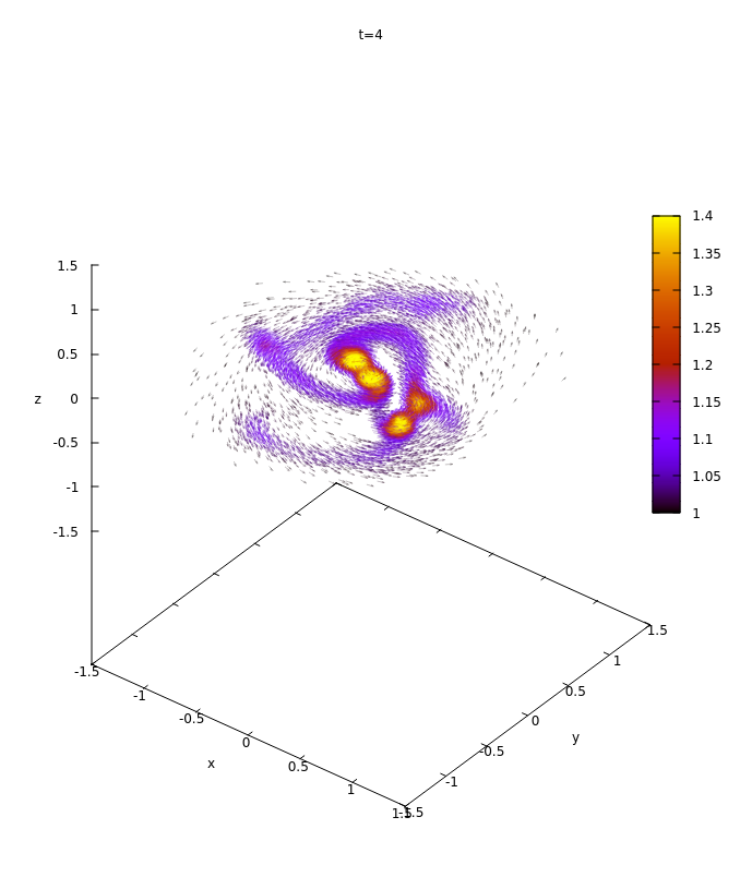
Figure 1: Isotropic simulation of the formation of a giant protostellar disc at t=4 (4096 time-steps). There are four protostars, but they are merging due to the resistance of the gas around them. The arrows denote the velocity field

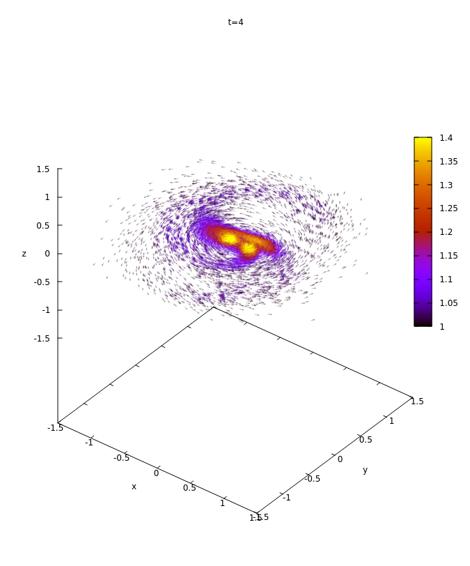
Figure 2: Anisotropic simulation of the formation of a giant protostellar disc at the same time of the previous figure, t=4 (4096 time-steps). There are three protostars, but they are merging due to the resistance of the gas around them, as in the isotropic case

Figures 1 and 2 show the disc formation at time $t=4$ (4096 time-steps) in both cases, isotropic and anisotropic respectively. At this time ($\sim$16 Myr) the system has collapsed to a giant protostellar disc with approximately 1 pc radius and $\sim 0.01$ pc thickness. Comparing both figures, one can see clearly that the isotropic simulation presents a smooth distribution of particles representing the disc’s isothermal component. On the other hand, anisotropic simulation is much more detailed and reveals the first stages of the isothermal disk fragmentation process. The four cores appearing in the isotropic simulation merges to form a solo core in the central part of the disc. The same happens to the three cores in the anisotropic case. The simulations could be more realistic if a gas-sweeping mechanism were introduced to mimic the effect of the protostellar wind. The color scale corresponds to the $\gamma$-index given in equation (88) where $\gamma=1$ (dark violet) stands for isothermal and $\gamma=1.4$ for adiabatic (yellow). The formed protostars appear in orange while the remnant debris are in light violet.

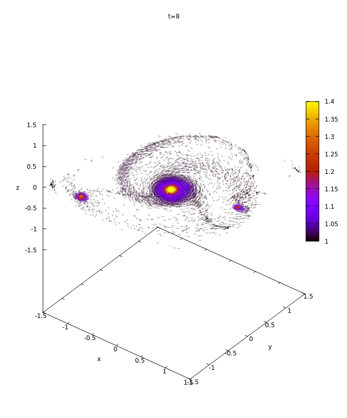
Figure 3: Isotropic simulation of the formation of a protostellar disc at t=8 (8192 time-steps)

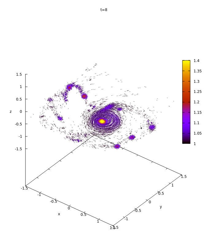
Figure 4: Anisotropic simulation of the formation of a protostellar disc at t=8 (8192 time-steps)

Figures 3 and 4 reveal the disc fragmentation at time $t=8$ ($8192$ time-steps, $\sim$40 Myr). In the isotropic case, Fig. 3, appear essentially two protostars, assuming the central object is the protostar, while in the anisotropic case, Fig. 4, one can count more than 10 protostars. Such protostars are self-gravitating lumps of gas in an intermediate state between isothermal and adiabatic, say $\gamma=1.25$.

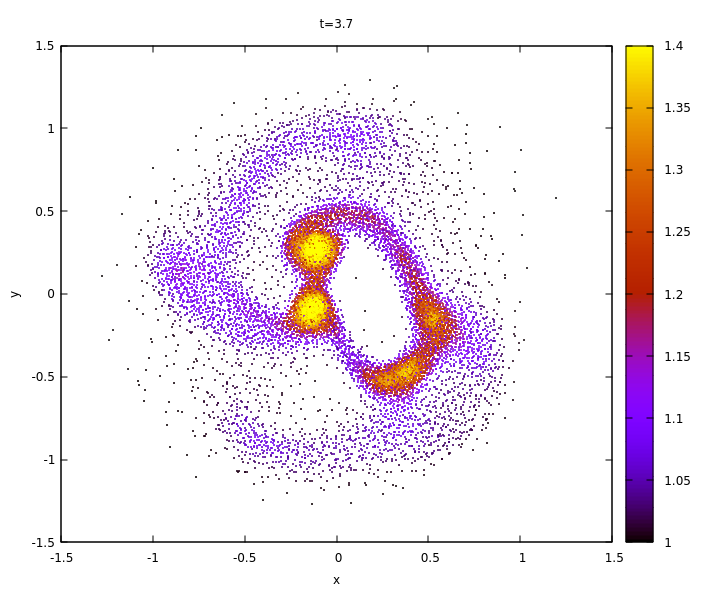
Figure 5: Isotropic case of the protostellar disc at t=3.7

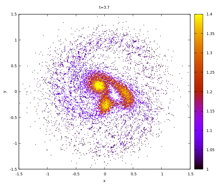
Figure 6: Anisotropic case of the protostellar disc at t=3.7 revealing filament-like fragments

Figures 5 and 6 show in more details the discrepant results among the isotropic and the anisotropic simulations, both at time $t=3.7$. In the latter, it is noticeable the large amount of filament-like fragments throughout the isothermal disc.

10 Discussion and conclusion

We have seen from the derivations made in Section 5 that the anisotropic SPH equations have an invariant aspect concerning the classic SPH interpolation equations, changing only the anisotropic kernel derivatives and the resulting spatial resolution of the simulations shown in the Sec. 9.

When the anisotropic results were compared with the isotropic ones for the first time, the impression left was that the anisotropic simulation was quite imprecise, allowing particles’ interpenetration. This apparent shock-overshooting did not seem intuitive since the artificial viscosity was designed to work effectively against the smoothing volume’s flattening direction. For example, a smoothing volume in the shock layer is expected to be an oblate ellipsoid whose smaller semi-axis has the normal direction of the shock front, which is, of course, the direction in which the artificial viscosity is maximum. It was then that, after reviewing the Rayleigh-Taylor instability, it became clear that the evolution of shock in the anisotropic case was more realistic than in the isotropic case. The adoption of isotropic smoothing prevents or mitigates the effects of such two-fluid instability.

The simulation of a rotating self-gravitating gas’s dissipative collapse evolved into a disc, thin on the inside and thick at the edges, similar to a protoplanetary disc. There was a relative loss of detail in the isotropic case. There was also much more formation of protostars in the anisotropic case due to the accretion shock’s necessary resolution in the rotating collapse’s critical phase. This result reinforces the idea that adopting anisotropic SPH simulations is fundamental, especially in astrophysics problems.

The use of smoothing volumes that adapt to the multivariate distribution of particles is equivalent to the MSVK method. In both methods, there was a favor in the formation of filaments since the smoothing ellipsoids tend to become prolate and aligned with the filaments. Likewise, the ongoing shock front is matched by the flattening of the ellipsoid in the shock direction. Thus, there is feedback in thinning both the filaments and the shock compared to isotropic simulations with spherical kernels.

The negative aspect of the proposed method is that it may be twice slower than the isotropic version, even when performing the non-gravitational simulation. This is due to the anisotropic artificial viscosity, which requires much shorter time steps according to Courant’s stability criteria. This is easy to understand because the artificial viscosity reaches very high values in the thin shock layers, or filamentary structures, in the direction of the smallest principal component due to the flattening or elongation of the ellipsoidal support of the kernel function, increasing the magnitude of the kernel gradient in the direction of the minor principal component.

An additional observation for anyone interested in testing or giving contributions to the present code is that it is a prototype, not optimized for bolder purposes, which would otherwise require a complete review regarding optimization for high-performance computing as, for instance, proposed by Marinho and Baldassin [2012]. Moreover, the code is a console version, so it has no graphics user interface. However, creating a graphical interface is relatively simple with the nowadays features, especially on UNIX / Linux platforms, using, for example, the interface utilities provided by the GTK Project (https://www.gtk.org/). The code is available under e-mailed request to pereira.marinho@unesp.br.

Appendix A B-spline kernel

The 3D version of the B-spline kernel can be written as

$$K_{\text{3D}}(\xi)=\frac{6}{\pi}\begin{cases}\frac{4}{3}-8\xi^{2}+8\xi^{3},&0\leq\xi\leq\frac{1}{2}\\ \frac{8}{3}(1-\xi)^{3},&\frac{1}{2}\leq\xi\leq 1\\ 0,&\xi\geq 1\end{cases}$$ (125)

so that the smoothing kernel is be computed by

$$W_{\mathbf{H}}(\bm{r})=\frac{1}{\text{det}\,\mathbf{H}}K_{\text{3D}}(\lvert\mathbf{H}^{-1}\bm{r}\rvert)$$ (126)

Usually, in the isotropic case, the smoothing length $h$ is such that the smoothing kernel function vanishes at a distance greater than or equal to twice the length, which means $r/(2h)=1$ for a spherical compact support. Here, the B-spline curve has been adjusted to zero at a distance $\lvert\mathbf{H}^{-1}\bm{r}\rvert=1$, which lies exactly on the surface of the ellipsoid hull under the replacement $r/(2h)\to\mathbf{H}^{-1}\bm{r}$.

References

- Appel [1985] Appel, A.W., 1985. An Efficient Program for Many-Body Simulation. SIAM Journal on Scientific and Statistical Computing 6, 85–103.
- Barnes and Hut [1986] Barnes, J., Hut, P., 1986. A hierarchical O(N log N) force-calculation algorithm. Nature 324, 446–449. doi:10.1038/324446a0.
- Bera et al. [2020] Bera, P., Jones, D.I., Andersson, N., 2020. Does elasticity stabilize a magnetic neutron star? Monthly Notices of the Royal Astronomical Society 499, 2636–2647. doi:10.1093/mnras/staa3015.
- Binney and Tremaine [1987] Binney, J., Tremaine, S., 1987. Galactic Dynamics. Princeton University Press.
- Braine, J. et al. [2020] Braine, J., Hughes, A., Rosolowsky, E., Gratier, P., Colombo, D., Meidt, S., Schinnerer, E., 2020. Rotation of molecular clouds in m 51. A&A 633, A17. URL: https://doi.org/10.1051/0004-6361/201834613, doi:10.1051/0004-6361/201834613.
- Braine, J. et al. [2018] Braine, J., Rosolowsky, E., Gratier, P., Corbelli, E., Schuster, K.-F., 2018. Properties and rotation of molecular clouds in m 33. A&A 612, A51. URL: https://doi.org/10.1051/0004-6361/201732405, doi:10.1051/0004-6361/201732405.
- Duda et al. [2001] Duda, R., Hart, P., Stork, D., 2001. Pattern Classification and Scene Analysis. Second ed., Wiley & Sons.
- Gingold and Monaghan [1977] Gingold, R.A., Monaghan, J.J., 1977. Smoothed particle hydrodynamics - Theory and application to non-spherical stars. Monthly Notices of the Royal Astronomical Society 181, 375–389. doi:10.1093/mnras/181.3.375.
- Hansen et al. [2004] Hansen, C.J., Kawaler, S.D., Trimble, V., 2004. Stellar Interiors: Physical Principles, Structure, and Evolution. Springer.
- Hernquist and Katz [1989] Hernquist, L., Katz, N., 1989. TREESPH - A unification of SPH with the hierarchical tree method. Astrophysical Journal Supplement Series 70, 419–446. doi:10.1086/191344.
- Kippenhahn et al. [2012] Kippenhahn, R., Weigert, A., Weiss, A., 2012. Stellar Structure and Evolution. Springer.
- Lucy [1977] Lucy, L.B., 1977. A numerical approach to the testing of the fission hypothesis. Astronomical Journal 82, 1013–1024. doi:10.1086/112164.
- Mahalanobis [1936] Mahalanobis, P.C., 1936. On the generalised distance in statistics 2, 49–55.
- Marinho [2014] Marinho, E.P., 2014. Pattern recognition issues on anisotropic smoothed particle hydrodynamics. Journal of Physics: Conference Series 490, 012063–012066. doi:10.1088/1742-6596/490/1/012063.
- Marinho and Andreazza [2010] Marinho, E.P., Andreazza, C.M., 2010. Computational Geometry (A). Asociación Argentina de Mecánica Computacional, Buenos Aires, Argentina. volume XXIX of Mecánica Computacional. chapter Anisotropic K-nearest Neighbor Search Using Covariance Quadtree. pp. 6045–6064.
- Marinho et al. [2001] Marinho, E.P., Andreazza, C.M., Lépine, J.R.D., 2001. SPH simulations of clumps formation by dissipative collisions of molecular clouds. II. Magnetic case. Astronomy and Astrophysics 379, 1123–1137. doi:10.1051/0004-6361:20011352.
- Marinho and Baldassin [2012] Marinho, E.P., Baldassin, A., 2012. Vectorized algorithms for quadtree construction and descent, in: Xiang, Y., Stojmenovic, I., Apduhan, B.O., Wang, G., Nakano, K., Zomaya, A. (Eds.), Algorithms and Architectures for Parallel Processing, Springer Berlin Heidelberg, Berlin, Heidelberg. pp. 69–82. doi:10.1007/978-3-642-33078-0_6.
- Marinho and Lépine [2000] Marinho, E.P., Lépine, J.R.D., 2000. SPH simulations of clumps formation by dissipative collision of molecular clouds. I. Non magnetic case. Astronomy and Astrophysics Supplement 142, 165–179. doi:10.1051/aas:2000327.
- Martel and Shapiro [2003] Martel, H., Shapiro, P.R., 2003. Cosmological Simulations with Adaptive Smoothed Particle Hydrodynamics, in: Makino, J., Hut, P. (Eds.), Astrophysical Supercomputing using Particle Simulations, p. 315.
- Martel et al. [1993] Martel, H., Shapiro, P.R., Villumsen, J.V., Kang, H., 1993. Adaptive Smoothed Particle Hydrodynamics with Application to Galaxy and Large-Scale Structure Formation. Memorie Della Societa Astronomica Italiana XX, 11pp.
- Mestel [2004] Mestel, L., 2004. Arthur Stanley Eddington: pioneer of stellar structure theory. Journal of Astronomical History and Heritage 7, 65–73.
- Monaghan [1994] Monaghan, J., 1994. Simulating free surface flows with sph. Journal of Computational Physics 110, 399 – 406. URL: http://www.sciencedirect.com/science/article/pii/S0021999184710345, doi:https://doi.org/10.1006/jcph.1994.1034.
- Monaghan [2012] Monaghan, J., 2012. Smoothed Particle Hydrodynamics and Its Diverse Applications. Annual Review of Fluid Mechanics 44, 323–346. doi:10.1146/annurev-fluid-120710-101220.
- Monaghan [1992] Monaghan, J.J., 1992. Smoothed Particle Hydrodynamics. Annual Review of Astronomy and Astrophysics 30, 543–574. doi:10.1146/annurev.aa.30.090192.002551.
- Monaghan and Gingold [1983] Monaghan, J.J., Gingold, R.A., 1983. Shock Simulation by the Particle Method SPH. Journal of Computational Physics 52, 374–389. doi:10.1016/0021-9991(83)90036-0.
- Owen et al. [1998] Owen, J.M., Villumsen, J.V., Shapiro, P.R., Martel, H., 1998. Adaptive Smoothed Particle Hydrodynamics : Methodology. II. The Astrophysical Journal Supplement Series 116, 155–209.
- Phillips [1999] Phillips, J.P., 1999. Astronomy and Astrophysics Supplement Series 134, 241–254.
- Shapiro et al. [1996] Shapiro, P.R., Martel, H., Villumsen, J.V., Owen, J.M., 1996. Adaptive Smoothed Particle Hydrodynamics, with Application to Cosmology: Methodology. The Astrophysical Journal Supplement Series 103, 269–330.
- York [2003] York, D.G., 2003. Interstellar matter, in: Meyers, R.A. (Ed.), Encyclopedia of Physical Science and Technology (Third Edition). third edition ed.. Academic Press, New York, p. 45–54. URL: https://www.sciencedirect.com/science/article/pii/B0122274105007171, doi:10.1016/B0-12-227410-5/00717-1.