The observed galaxy power spectrum in General Relativity

Emanuele Castorina11footnotetext: Author names are listed alphabetically.    and Enea Di Dio
Abstract

Measurements of the clustering of galaxies in Fourier space, and at low wavenumbers, offer a window into the early Universe via the possible presence of scale dependent bias generated by Primordial Non Gaussianites. On such large scales a Newtonian treatment of density perturbations might not be sufficient to describe the measurements, and a fully relativistic calculation should be employed. The interpretation of the data is thus further complicated by the fact that relativistic effects break statistical homogeneity and isotropy and are potentially divergent in the Infra-Red (IR). In this work we compute for the first time the ensemble average of the most used Fourier space estimator in spectroscopic surveys, including all general relativistic (GR) effects, and allowing for an arbitrary choice of angular and radial selection functions. We show that any observable is free of IR sensitivity once all the GR terms, individually divergent, are taken into account, and that this cancellation is a consequence of the presence of the Weinberg adiabatic mode as a solution to Einstein’s equations. We then study the importance of GR effects, including lensing magnification, in the interpretation of the galaxy power spectrum multipoles, finding that they are in general a small, less than ten percent level, correction to the leading redshift space distortions term. This work represents the baseline for future investigations of the interplay between Primordial Non Gaussianities and GR effects on large scales and in Fourier space.

CERN-TH-2021-087

1 Introduction

The cosmological interpretation of galaxy clustering data is complicated by the fact we observe the angular position and redshift of the galaxies, rather than their true physical position on the lightcone. The mapping between these two systems of coordinates is distorted by a number of observational effects.

The most important one is Redshift Space Distortions (RSD), i.e. the contribution of the galaxies peculiar velocity, projected along the line of sight (LOS), to their observed redshift. RSD select the observer’s location as a special place and therefore break the isotropy and homogeneity of n𝑛nth-point correlation functions. On the other hand, RSD give access to information about the velocity field we would not be able to retrieve otherwise.

Other observational effects, arising from the perturbation of the observed redshifts and angles, are proportional to the gravitational potential or its gradient and are therefore suppressed on sub-horizon scales with respect to the underlying dark matter density field, while becoming important only on very large scales. The relevant dimensionful parameter is the Hubble scale, which separates sub-horizon modes where Netwonian physics applies from the super-horizon scales where the full General Relativity machinery is at work. For this reason these observational features are usually called general relativistic (GR) effects111 Let us remark that Einstein’s equations are not required to derive the relativistic galaxy number counts, see Refs. [Yoo:2009, Yoo:2010, Challinor:2011bk, Bonvin:2011bg, Jeong:2011as]. However the cancellation of the infrared divergences discussed in this work relies on the existence of the Weinberg adiabatic mode [Weinberg:2003sw] as a solution of linearized Einstein’s field equations.. Examples of GR effects are lensing, doppler magnification and the Integrated Sachs-Wolfe (ISW) effect. Galaxy clustering in a relativistic framework has been first derived in Refs. [Yoo:2009, Yoo:2010, Challinor:2011bk, Bonvin:2011bg, Jeong:2011as] in linear perturbation theory and then extended to higher orders in Refs. [Yoo:2014sfa, Bertacca:2014dra, DiDio:2014lka, DiDio:2018zmk, DiDio:2020jvo]. It has been also generalized to vector perturbations [Durrer:2016jzq], non-flat FLRW universe [DiDio:2016ykq], intensity mapping [Hall:2012wd] and Ly-α𝛼\alpha forest [Irsic:2015nla] observables.

GR effects are important for two main reasons. The first one is that they provide a fully gauge-invariant framework to test gravity on the largest scales. Secondly, GR effects could be a contaminant to measurements of local Primordial Non Gaussianities (PNG) in the clustering of galaxies with scale dependent bias [Dalal:2008, Matarrese:2008, Slosar:2008hx, Desjacques:2010jw]. Local PNG appear as large scale divergences, proportional to the primordial gravitational potential, in the clustering of biased tracers. Local PNG arise from the coupling between the large and small scale modes generated during inflation, and in the squeezed limit they cannot be generated by the dynamics of GR at later times. However, projection effects, like the GR effects responsible for the mapping between true and observed coordinates, could mimic PNG, since they also contain terms proportional to the gravitational potential. The literature on the subject is vast: for photometric surveys measuring angular power spectra, marginalizing over the unknown free parameters that enter the full GR expression causes significant degradation of the error on local PNG [Camera:2014bwa, Alonso:2015sfa, Fonseca:2015laa, Raccanelli:2015GR]. This is in part due to GR effects contributing mostly to the cross correlation between different redshift bins, which would be zero in a standard Newtonian approach. In Fourier-space (but in plane-parallel approximation and neglecting integrated effects)Ref. [Yoo:2012se] concluded that the degeneracy is reduced, especially if one is able to set priors on evolution and magnification biases, due to the different redshift evolution between local PNG and relativistic effects. A deeper understanding of this issue is therefore of utmost importance for future surveys that could improve over current CMB [plancknG] and Large-Scale Structure [Castorina2019] constraints by an order of magnitude [spherex].

On this topic, it has been recently argued in [Grimm:2020ays] that GR effects do not produce any PNG-like feature at large scales in the galaxy power spectrum. This is interpreted as a consequence of the equivalence principle. The cancellation of these terms holds for the variance of the galaxy density field, and for a galaxy power spectrum the authors in [Grimm:2020ays] define such that its variance corresponds to the observed one.

The goal of this work is to clarify on the issue of whether GR effects could be degenerate with a measurement of local PNG. We will confirm the result in [Grimm:2020ays] for the variance of the galaxy density field, but at the same time we will show the power spectrum as defined in [Grimm:2020ays] is not observable, and that true observed power spectrum as estimated in galaxy redshift surveys receives contributions proportional to the gravitational potential even in the absence of PNG. However, these terms do not show any sensitivity to long wavelength modes, which we will demonstrate is a consequence of the equivalence principle and of the existence of Weinberg adiabatic modes [Weinberg:2003sw]. Contributions to the power spectrum arising from local PNG are instead genuinely sensitive long wavelength modes. For the first time we will also include observational effects like an arbitrary survey geometry and selection function when discussing the importance of GR effects on the power spectrum. Differently than previous analyses in Fourier space, our approach will include also wide-angle and evolution effects consistently.

This paper is organized as follows. In section 2 we introduce the power spectrum estimator and we discuss its interpretation and its connection to the theoretical modeling. In section 3 we describe the fully relativistic galaxy number counts and then in section 4 we discuss the cancellation of the IR divergences in the correlation function. In section 5 we compute the power spectrum including all the relativistic effects and then we conclude in section 6. Several appendices contain the details about azimuthally symmetric window functions (App. A), the full relativistic correlation function (App. B) and the contribution of the observer velocity (App. C).

In this work we adopt the following Fourier convention for the Fourier transform

f(𝐱)=d3k(2π)3f(𝐤)ei𝐱𝐤,f(𝐤)=d3xf(𝐱)ei𝐱𝐤,formulae-sequence𝑓𝐱superscriptd3𝑘superscript2𝜋3𝑓𝐤superscript𝑒𝑖𝐱𝐤𝑓𝐤superscriptd3𝑥𝑓𝐱superscript𝑒𝑖𝐱𝐤f\left({\bf{x}}\right)=\int\frac{{\rm d}^{3}k}{\left(2\pi\right)^{3}}f\left({\bf{k}}\right)e^{i{\bf{x}}\cdot{\bf{k}}}\,,\qquad f\left({\bf{k}}\right)=\int{\rm d}^{3}xf\left({\bf{x}}\right)e^{-i{\bf{x}}\cdot{\bf{k}}}\,, (1.1)

and the Hankel transform

ξ(s)=idk2π2k2P(k)j(ks),P(k)=4π(i)dss2ξ(s)j(ks).formulae-sequencesubscript𝜉𝑠superscript𝑖d𝑘2superscript𝜋2superscript𝑘2subscript𝑃𝑘subscript𝑗𝑘𝑠subscript𝑃𝑘4𝜋superscript𝑖differential-d𝑠superscript𝑠2subscript𝜉𝑠subscript𝑗𝑘𝑠\xi_{\ell}\left(s\right)=i^{\ell}\int\frac{{\rm d}k}{2\pi^{2}}k^{2}P_{\ell}\left(k\right)j_{\ell}\left(ks\right)\,,\qquad P_{\ell}\left(k\right)=4\pi\left(-i\right)^{\ell}\int{\rm d}ss^{2}\xi_{\ell}\left(s\right)j_{\ell}\left(ks\right)\,. (1.2)

2 The power spectrum estimator

Given a catalog N(𝐧,z)𝑁𝐧𝑧N(\mathbf{n},z) of galaxy positions in the sky, 𝐧𝐧\mathbf{n}, and redshifts z𝑧z, we have several ways to construct a quadratic estimator of the data. For the remainder of this work we will focus on spectroscopic surveys, where redshift accuracy is obtained for each object in the catalog. If one wants to work in the observed coordinates, then a spherical harmonics approach leads to the measurements of as many angular power spectra as redshifts bins of the data (plus their cross correlation). The advantage of this approach is that the implementation of GR effects is simple and there is no need to assume a fiducial cosmology to perform the measurements, the so called Alcock-Pacinski effect [AP] 222We have efficient and accurate numerical tools to compute the redshift-dependent angular power spectra including all the relativistic effects: class [Blas:2011rf, DiDio:2013bqa, Schoneberg:2018fis] and cambsource [Challinor:2011bk].. There are two main drawbacks of using angular power spectra. The first one is that, to achieve optimal signal extraction, the number of redshift bins has to be extremely large, see for instance Refs. [Asorey:2012rd, DiDio:2013sea]. This is more of a concern for small scales analysis than for PNG ones, however in the latter case one has to compute the cross correlation between all the different bins. This results in a large data vector, which makes the estimation of the covariance matrix of the data a challenging task. The second problem is that the connection to the perturbative approaches beyond linear theory, required to properly model the small scales, is non trivial333See [Castorina2018, Jalilvand19] for a recent solution to this issue.. Similar conclusions hold for spherical-Fourier-Bessel (sFB) methods [Fisher94, HT95, Tadros99, Percival2004, Rassat:2011aa, Yoo:2013tc, Samushia, Gebhardt21], where the redshift coordinate is radially Fourier transformed.

The other main option to build a quadratic estimator of the data is to work in a 3D coordinate system and measure the two-point correlation function or the power spectrum. This approach assumes a fiducial cosmology to convert angular positions and redshifts into distances. This causes no loss of information, but it requires some care if the assumed fiducial cosmology is very different than the true underlying one. That is however not a worry since Planck [Aghanim:2018eyx] and BAO [Auburg2015, Alam:2020sor] measurements have constrained the distance-redshift relation to a few percent. The advantages of 3D methods are the straightforward connection to perturbation theory and the reduced dimensionality of data vector, comprising of approximately 100 data points. The main drawback of 3D estimators is that GR effects are not easily implemented, especially the ones integrated along the line of sight, like lensing magnification, ISW and time-delay. One of the main goal of this work is to resolve this issue as well, providing the exact interpretation of the estimator of the power spectrum. Due to its practical advantages and robust theoretical interpretation the 3D methods should be preferred in spectroscopic surveys, and Fourier ones in particular to constraints on PNG.

A generic estimator for the multipoles of the power spectrum can be written by summing over all pairs of galaxies with the appropriate Fourier phases,

P^L(k)=2L+1AdΩ𝐤4πd3s1d3s2Δ(𝐬1)Δ(𝐬2)ϕ(𝐬1)ϕ(𝐬2)ei𝐤(𝐬1𝐬2)L(𝐤^𝐝^LOS),subscript^𝑃𝐿𝑘2𝐿1𝐴𝑑subscriptΩ𝐤4𝜋superscriptd3subscript𝑠1superscriptd3subscript𝑠2Δsubscript𝐬1Δsubscript𝐬2italic-ϕsubscript𝐬1italic-ϕsubscript𝐬2superscript𝑒𝑖𝐤subscript𝐬1subscript𝐬2subscript𝐿^𝐤subscript^𝐝LOS\hat{P}_{L}\left(k\right)=\frac{2L+1}{A}\int\frac{d\Omega_{\bf{k}}}{4\pi}\int{\rm d}^{3}s_{1}{\rm d}^{3}s_{2}\,\Delta\left({\bf{s}}_{1}\right)\Delta\left({\bf{s}}_{2}\right)\phi\left({\bf{s}}_{1}\right)\phi\left({\bf{s}}_{2}\right)e^{i{\bf{k}}\cdot\left({\bf{s}}_{1}-{\bf{s}}_{2}\right)}\mathcal{L}_{L}\left(\hat{\bf{k}}\cdot\hat{\bf{d}}_{\rm LOS}\right)\,, (2.1)

where A𝐴A is a normalisation constant, Δ(𝐬)Δ𝐬\Delta({\bf{s}}) denotes the galaxy density contrast, ϕ(𝐬)italic-ϕ𝐬\phi\left({\bf{s}}\right) is the survey window function, and Lsubscript𝐿\mathcal{L}_{L} is the Legendre polynomial of order L𝐿L. This is the so called Yamamoto estimator [Yamamoto:2005dz], which reduces to the FKP estimator [FKP] for L=0𝐿0L=0. Beyond the monopole, the estimator depends explicitly on the choice of the line of sight, 𝐝LOSsubscript𝐝LOS{\bf{d}}_{\rm LOS}, for the pair of galaxies at 𝐬1subscript𝐬1\mathbf{s}_{1} and 𝐬2subscript𝐬2\mathbf{s}_{2}.

For an unbiased estimate of cosmological parameters it is therefore of utmost importance to first understand the relation between the average of the estimator and the analytical prediction. Some of the following considerations have appeared elsewhere before [Castorina:2017inr, Scoccimarro2015], but we report them here for clarity. In Section 1 we said that RSD, and other GR effects, break homogeneity and isotropy of correlation functions, making for instance the power spectrum of the observed galaxy density field non-diagonal. This means that if we Fourier Transform Δ[𝐬(𝐧,z)]Δdelimited-[]𝐬𝐧𝑧\Delta[{\bf{s}}(\mathbf{n},z)] to Δ(𝐤)Δ𝐤\Delta(\mathbf{k}), we obtain

Δ(𝐤1)Δ(𝐤2)P(𝐤1,𝐤2),delimited-⟨⟩Δsubscript𝐤1Δsubscript𝐤2𝑃subscript𝐤1subscript𝐤2\displaystyle\left\langle\,\Delta(\mathbf{k}_{1})\Delta(\mathbf{k}_{2})\,\right\rangle\equiv P(\mathbf{k}_{1},\mathbf{k}_{2})\,, (2.2)

while the Yamamoto estimator defined above is a function of a single wavenumber k𝑘k. We will now show that the relation of P(𝐤1,𝐤2)𝑃subscript𝐤1subscript𝐤2P(\mathbf{k}_{1},\mathbf{k}_{2}) with P^L(k)subscript^𝑃𝐿𝑘\hat{P}_{L}\left(k\right) is LOS-dependent. Consider first the midpoint as the line of sight, 𝐝LOS=𝐝m(𝐬1+𝐬2)/2subscript𝐝LOSsubscript𝐝msubscript𝐬1subscript𝐬22{\bf{d}}_{\rm LOS}={\bf{d}}_{\rm m}\equiv({\bf{s}}_{1}+{\bf{s}}_{2})/2, and assume that the window function is equal to unity everywhere inside the survey volume, which we take to cover the whole sky. It is easy to see that in this case the average of the estimator is given by [Scoccimarro2015, Castorina:2017inr]

P^L(k)=delimited-⟨⟩subscript^𝑃𝐿𝑘absent\displaystyle\left\langle\,\hat{P}_{L}(k)\,\right\rangle= (2L+1)Ad3dmd3q(2π)3ei𝐪𝐝m2𝐿1𝐴superscriptd3subscript𝑑msuperscriptd3𝑞superscript2𝜋3superscript𝑒𝑖𝐪subscript𝐝m\displaystyle\frac{(2L+1)}{A}\int\mathrm{d}^{3}d_{\rm m}\,\int\frac{\mathrm{d}^{3}q}{(2\pi)^{3}}e^{i\mathbf{q}\cdot\mathbf{d}_{\rm m}}
×dΩ𝐤4πP(𝐤+𝐪/2,𝐤+𝐪/2)L(𝐤^𝐝^m),\displaystyle\times\int\frac{\mathrm{d}\Omega_{\mathbf{k}}}{4\pi}P(\mathbf{k}+\mathbf{q}/2,-\mathbf{k}+\mathbf{q}/2)\mathcal{L}_{L}(\hat{\mathbf{k}}\cdot\hat{\mathbf{d}}_{\rm m})\,, (2.3)

revealing that the Yamamoto estimator further compresses the underlying power spectrum by averaging over the wavenumber 𝐪𝐪\mathbf{q} associated to the line of sight 𝐝msubscript𝐝𝑚\mathbf{d}_{m}. Another possible choice for the line of sight is one of the two pair members, 𝐝LOS=𝐬1subscript𝐝LOSsubscript𝐬1{\bf{d}}_{\rm LOS}={\bf{s}}_{1}, usually called the endpoint line of sight. In this case

P^L(k)=2L+1AdΩ𝐤4πd3s1d3q(2π)3P(𝐪𝐤,𝐤)ei𝐪𝐬1L(𝐤^𝐬^1),delimited-⟨⟩subscript^𝑃𝐿𝑘2𝐿1𝐴dsubscriptΩ𝐤4𝜋superscriptd3subscript𝑠1superscriptd3𝑞superscript2𝜋3𝑃𝐪𝐤𝐤superscript𝑒𝑖𝐪subscript𝐬1subscript𝐿^𝐤subscript^𝐬1\left\langle\,\hat{P}_{L}\left(k\right)\,\right\rangle=\frac{2L+1}{A}\int\frac{{\rm d}\Omega_{\mathbf{k}}}{4\pi}\int{\rm d}^{3}s_{1}\int\frac{{\rm d}^{3}q}{\left(2\pi\right)^{3}}\,P\left({\bf{q}}-{\bf{k}},{\bf{k}}\right)e^{i{\bf{q}}\cdot{\bf{s}}_{1}}\mathcal{L}_{L}\left(\hat{\bf{k}}\cdot\hat{\bf{s}}_{1}\right), (2.4)

which shows how different choices of LOS result in different weighting of the momentum 𝐪𝐪\mathbf{q}.

A more compact expression for the average of the estimator can be obtained by noticing that the configuration space two-point correlation function depends on the triangle formed by the observer and the pair of galaxies

Δ(𝐬1)Δ(𝐬2)ξ(𝐬2𝐬1,𝐝LOS)delimited-⟨⟩Δsubscript𝐬1Δsubscript𝐬2𝜉subscript𝐬2subscript𝐬1subscript𝐝LOS\displaystyle\left\langle\,\Delta(\mathbf{s}_{1})\Delta(\mathbf{s}_{2})\,\right\rangle\equiv\xi(\mathbf{s}_{2}-\mathbf{s}_{1},\mathbf{d}_{\rm LOS})\, (2.5)

and it can therefore be formally Fourier transformed with respect to 𝐬𝐬2𝐬1𝐬subscript𝐬2subscript𝐬1\mathbf{s}\equiv\mathbf{s}_{2}-\mathbf{s}_{1} to define a LOS dependent power spectrum

P(𝐤,𝐝LOS)d3sei𝐤𝐬ξ(𝐬,𝐝LOS).𝑃𝐤subscript𝐝LOSsuperscriptd3𝑠superscript𝑒𝑖𝐤𝐬𝜉𝐬subscript𝐝LOS\displaystyle P(\mathbf{k},\mathbf{d}_{\rm LOS})\equiv\int{\rm d}^{3}s\,e^{-i\mathbf{k}\cdot\mathbf{s}}\xi(\mathbf{s},\mathbf{d}_{\rm LOS})\,. (2.6)

The Yamamoto estimator is then the LOS average of the LOS dependent power spectrum

P^L(k)=(2L+1)AdΩ𝐤4πd3dLOSP(𝐤,𝐝LOS)L(𝐤^𝐝^LOS).delimited-⟨⟩subscript^𝑃𝐿𝑘2𝐿1𝐴dsubscriptΩ𝐤4𝜋superscriptd3subscript𝑑LOS𝑃𝐤subscript𝐝LOSsubscript𝐿^𝐤subscript^𝐝LOS\displaystyle\left\langle\,\hat{P}_{L}(k)\,\right\rangle=\frac{(2L+1)}{A}\int\frac{\mathrm{d}\Omega_{\mathbf{k}}}{4\pi}\,\int\mathrm{d}^{3}d_{\rm LOS}\,P(\mathbf{k},\mathbf{d}_{\rm LOS})\mathcal{L}_{L}(\hat{\mathbf{k}}\cdot\hat{\mathbf{d}}_{\rm LOS})\,. (2.7)

The above expression also clarifies how to take the plane-parallel limit of the estimator [Castorina:2017inr].

2.1 The convolution with a window function

For practical reasons the choice 𝐝LOS=𝐬1subscript𝐝LOSsubscript𝐬1{\bf{d}}_{\rm LOS}={\bf{s}}_{1} is usually preferred [Bianchi2015, Scoccimarro2015, Hand2017], since it requires fewer Fourier Transforms than the identification of the LOS as the bisector between the two galaxies and the observer [Castorina:2017inr]. We shall use this choice, usually referred as the endpoint LOS in the literature, for the remainder of this work. Although not strictly necessary, in our implementation we will assume that the window function can be separated into a radial and angular part, i.e. ϕ(𝐬)=ϕ(s)W(𝐬^)italic-ϕ𝐬italic-ϕ𝑠𝑊^𝐬\phi(\mathbf{s})=\phi(s)W(\hat{\mathbf{s}}). Generalizations to non-separable masks are straightforward. If we start from the following decomposition for the two-point correlation function

ξ(𝐬,𝐬1)=ξ(s,s1)(μ),𝜉𝐬subscript𝐬1subscriptsubscript𝜉𝑠subscript𝑠1subscript𝜇\displaystyle\xi(\mathbf{s},\mathbf{s}_{1})=\sum_{\ell}\xi_{\ell}(s,s_{1})\cal{L}_{\ell}(\mu)\,, (2.8)

with μ𝐬^𝐬^1𝜇^𝐬subscript^𝐬1\mu\equiv\hat{\mathbf{s}}\cdot\hat{\mathbf{s}}_{1}, we arrive to a compact expression for the expectation value of the Yamamoto estimator

P^L(k)delimited-⟨⟩subscript^𝑃𝐿𝑘\displaystyle\langle\hat{P}_{L}\left(k\right)\rangle =\displaystyle= 2L+1A(i)Ld3s1d3sξ(s,s1)(𝐬^1𝐬^)L(𝐬^𝐬^1)jL(ks)ϕ(𝐬1)ϕ(𝐬2)2𝐿1𝐴subscriptsuperscript𝑖𝐿superscriptd3subscript𝑠1superscriptd3𝑠subscript𝜉𝑠subscript𝑠1subscriptsubscript^𝐬1^𝐬subscript𝐿^𝐬subscript^𝐬1subscript𝑗𝐿𝑘𝑠italic-ϕsubscript𝐬1italic-ϕsubscript𝐬2\displaystyle\frac{2L+1}{A}\sum_{\ell}\left(-i\right)^{L}\int{\rm d}^{3}s_{1}{\rm d}^{3}s\xi_{\ell}\left(s,s_{1}\right)\mathcal{L}_{\ell}\left(\hat{\bf{s}}_{1}\cdot\hat{\bf{s}}\right)\mathcal{L}_{L}\left(\hat{\bf{s}}\cdot\hat{\bf{s}}_{1}\right)j_{L}\left(ks\right)\phi\left({\bf{s}}_{1}\right)\phi\left({\bf{s}}_{2}\right)
=\displaystyle= 2L+1A1(i)L(L1000)2(21+1)2𝐿1𝐴subscriptsubscript1superscript𝑖𝐿superscript𝐿subscript100022subscript11\displaystyle\frac{2L+1}{A}\sum_{\ell\ell_{1}}\left(-i\right)^{L}\left(\begin{array}[]{ccc}L&\ell&\ell_{1}\\ 0&0&0\end{array}\right)^{2}\left(2\ell_{1}+1\right)
d3s1d3sξ(s,s1)1(𝐬^𝐬^1)jL(ks)ϕ(𝐬1)ϕ(𝐬2)superscriptd3subscript𝑠1superscriptd3𝑠subscript𝜉𝑠subscript𝑠1subscriptsubscript1^𝐬subscript^𝐬1subscript𝑗𝐿𝑘𝑠italic-ϕsubscript𝐬1italic-ϕsubscript𝐬2\displaystyle\qquad\int{\rm d}^{3}s_{1}{\rm d}^{3}s\xi_{\ell}\left(s,s_{1}\right)\mathcal{L}_{\ell_{1}}\left(\hat{\bf{s}}\cdot\hat{\bf{s}}_{1}\right)j_{L}\left(ks\right)\phi\left({\bf{s}}_{1}\right)\phi\left({\bf{s}}_{2}\right)
=\displaystyle= 2L+1A,1(i)L(L1000)2(21+1)2𝐿1𝐴subscriptsubscript1superscript𝑖𝐿superscript𝐿subscript100022subscript11\displaystyle\frac{2L+1}{A}\sum_{\ell,\ell_{1}}\left(-i\right)^{L}\left(\begin{array}[]{ccc}L&\ell&\ell_{1}\\ 0&0&0\end{array}\right)^{2}\left(2\ell_{1}+1\right) (2.15)
ds1s12dss2ξ(s,s1)jL(ks)ϕ(s1)F1(s1,s),differential-dsubscript𝑠1superscriptsubscript𝑠12differential-d𝑠superscript𝑠2subscript𝜉𝑠subscript𝑠1subscript𝑗𝐿𝑘𝑠italic-ϕsubscript𝑠1subscript𝐹subscript1subscript𝑠1𝑠\displaystyle\qquad\int{\rm d}s_{1}s_{1}^{2}{\rm d}ss^{2}\xi_{\ell}\left(s,s_{1}\right)j_{L}\left(ks\right)\phi\left(s_{1}\right)F_{\ell_{1}}\left(s_{1},s\right)\,,

where we have introduced

F1(s1,s)=dΩ𝐬^dΩ𝐬^1ϕ(s2)W(𝐬^1)W(𝐬^2)1(𝐬^1𝐬^).subscript𝐹subscript1subscript𝑠1𝑠differential-dsubscriptΩ^𝐬differential-dsubscriptΩsubscript^𝐬1italic-ϕsubscript𝑠2𝑊subscript^𝐬1𝑊subscript^𝐬2subscriptsubscript1subscript^𝐬1^𝐬F_{\ell_{1}}\left(s_{1},s\right)=\int{\rm d}\Omega_{\hat{\bf{s}}}{\rm d}\Omega_{\hat{\bf{s}}_{1}}\phi\left(s_{2}\right)W\left(\hat{\bf{s}}_{1}\right)W\left(\hat{\bf{s}}_{2}\right)\mathcal{L}_{\ell_{1}}\left(\hat{\bf{s}}_{1}\cdot\hat{\bf{s}}\right)\,. (2.16)

The integration variable s1subscript𝑠1s_{1} serves to keep track of the redshift evolution of the sample within the survey, and of the different dependence of the GR effects on the distance between the observer and the galaxies. In real surveys the functions F(s1,s)subscript𝐹subscript𝑠1𝑠F_{\ell}(s_{1},s) can be estimated using traditional pair counting algorithms or Fast Fourier Transforms (FFT).

2.1.1 The effective redshift

A useful approximation often employed in the literature is to assume that the theoretical prediction can be computed at some effective redshift. This allows to take the correlation function multipoles outside of the ds1dsubscript𝑠1{\rm d}s_{1} integral in Eq. (2.1), that can be computed once and for all over the window function multipoles Fsubscript𝐹F_{\ell}. The effective redshift approximation is motivated by the fact that we are mostly interested in the clustering at separations much smaller than the comoving distance associated to the redshift of the individual galaxies, that can therefore be modeled at the same redshift. On the small scales relevant for BAO and RSD this has been shown to be an excellent approximation [Vlah2016], as well for PNG studies on small patches of the sky [Castorina2019]. To see how this works let us assume that the correlation function can be written as a sum over different terms, each of them being the correlation function between two operators 𝒪𝒪\cal{O} and 𝒪superscript𝒪\cal{O}^{\prime} entering the expansion of the galaxy density field,

ξ(s,s1)𝒪𝒪ξ,𝒪𝒪(s,s1).subscript𝜉𝑠subscript𝑠1subscript𝒪superscript𝒪subscript𝜉𝒪superscript𝒪𝑠subscript𝑠1\displaystyle\xi_{\ell}(s,s_{1})\equiv\sum_{\cal{O}\cal{O}^{\prime}}\xi_{\ell,\cal{O}\cal{O}^{\prime}}(s,s_{1})\,. (2.17)

For each contribution to the correlation function we could therefore choose an effective redshift such that at a given, small enough, reference separation s~~𝑠\tilde{s}, the model evaluated at this suitably defined redshift exactly matches the full prediction in Eq. (2.1). In practice, at small scales the correlation function is dominated by the Newtonian terms in the plane parallel limit, that allows us to define a single effective redshift for each multipole

ξ,(s~,zeff,)d3s1ξ(s~,s1)ϕ(s1)2W(s^1)2d3s1ϕ(s1)2W(s^1)2.subscript𝜉~𝑠subscript𝑧effsuperscriptd3subscript𝑠1subscript𝜉~𝑠subscript𝑠1italic-ϕsuperscriptsubscript𝑠12𝑊superscriptsubscript^𝑠12superscriptd3subscript𝑠1italic-ϕsuperscriptsubscript𝑠12𝑊superscriptsubscript^𝑠12\displaystyle\xi_{\ell,}(\tilde{s},z_{\rm eff,\ell})\equiv\frac{\int{\rm d}^{3}s_{1}\,\xi_{\ell}(\tilde{s},s_{1})\phi(s_{1})^{2}W(\hat{s}_{1})^{2}}{\int{\rm d}^{3}s_{1}\,\phi(s_{1})^{2}W(\hat{s}_{1})^{2}}\,. (2.18)

Notice this operation is always possible as long as the transfer function and the growth factors are separable. Under the effective redshift approximation the average of the Yamamoto estimator reads

P^L(k)=delimited-⟨⟩subscript^𝑃𝐿𝑘absent\displaystyle\left\langle\,\hat{P}_{L}(k)\,\right\rangle= 2L+1A,1(i)L(L1000)2(21+1)dss2ξ(s,zeff,)jL(ks)2𝐿1𝐴subscriptsubscript1superscript𝑖𝐿superscript𝐿subscript100022subscript11differential-d𝑠superscript𝑠2subscript𝜉𝑠subscript𝑧effsubscript𝑗𝐿𝑘𝑠\displaystyle\frac{2L+1}{A}\sum_{\ell,\ell_{1}}\left(-i\right)^{L}\left(\begin{array}[]{ccc}L&\ell&\ell_{1}\\ 0&0&0\end{array}\right)^{2}\left(2\ell_{1}+1\right)\int{\rm d}ss^{2}\,\xi_{\ell}\left(s,z_{\rm eff,\ell}\right)j_{L}\left(ks\right) (2.21)
×ds1s12ϕ(s1)F1(s1,s)\displaystyle\times\int{\rm d}s_{1}s_{1}^{2}\,\phi\left(s_{1}\right)F_{\ell_{1}}\left(s_{1},s\right)
\displaystyle\equiv 2L+1A,1(i)L(L1000)2dss2ξ(s,zeff,)jL(ks)Q1(s).2𝐿1𝐴subscriptsubscript1superscript𝑖𝐿superscript𝐿subscript10002differential-d𝑠superscript𝑠2subscript𝜉𝑠subscript𝑧effsubscript𝑗𝐿𝑘𝑠subscript𝑄subscript1𝑠\displaystyle\frac{2L+1}{A}\sum_{\ell,\ell_{1}}\left(-i\right)^{L}\left(\begin{array}[]{ccc}L&\ell&\ell_{1}\\ 0&0&0\end{array}\right)^{2}\int{\rm d}s\,s^{2}\xi_{\ell}\left(s,z_{\rm eff,\ell}\right)j_{L}\left(ks\right)Q_{\ell_{1}}(s)\,. (2.24)

The functions Q1subscript𝑄subscript1Q_{\ell_{1}} can be easily estimated using FFT methods [Beutler:2018vpe]. It is often the case that the different multipoles have very similar zeff,subscript𝑧effz_{\rm eff,\ell}, and therefore a common effective redshift is defined for the entire correlation function444Another possible definition is the pair weighted effective redshifts, see for example [deMattia:2020fkb].,

zeff=d3sϕ(s)2W(s^)2z(s)d3sϕ(s)2W(s^)2.subscript𝑧effsuperscriptd3𝑠italic-ϕsuperscript𝑠2𝑊superscript^𝑠2𝑧𝑠superscriptd3𝑠italic-ϕsuperscript𝑠2𝑊superscript^𝑠2\displaystyle z_{\rm eff}=\frac{\int{\rm d}^{3}s\,\phi(s)^{2}W(\hat{s})^{2}z(s)}{\int{\rm d}^{3}s\,\phi(s)^{2}W(\hat{s})^{2}}\,. (2.25)

The definition above does not guarantee that the small scale power spectrum evaluated at zeffsubscript𝑧effz_{\rm eff} converges to the true answer, but the difference can usually be reabsorbed by changing the value of the unknown bias parameters. A global definition is also more prone to anisotropies in the orientation of galaxy pairs in the survey, which could also bias the theoretical prediction, as recently pointed out in [Obuljen:2021ryv].

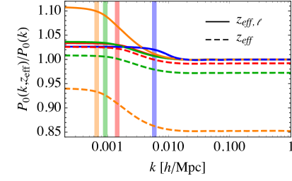
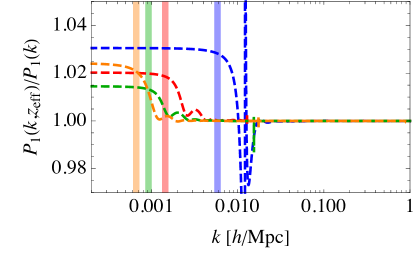
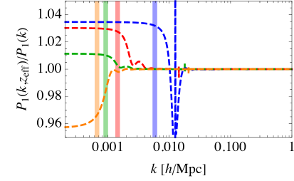
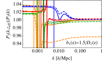
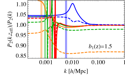
The simple picture described above is complicated by those correlation function terms which are integrated along the LOS, like lensing magnification and ISW. In this case, the definition of effective redshift given above does not strictly hold. Nevertheless we will see in the next sections (see Figs. 4 and 10) that our choices in Eqs. (2.18, 2.25) are accurate enough for these terms as well, vastly simplifying the convolution with the window function.

2.1.2 The Integral Constraint

In redshift surveys the mean number density of the underlying galaxy population is usually not known a priori, and it is estimated from the data themselves. The resulting overdensity will therefore vanish when integrated over the entire volume of the survey, an effect known as the Integral Constraint (IC). In addition, if the redshift selection function is also estimated from the data, the overdensity has to vanish in radial bins when averaging over the angular footprint. This is the so called Radial Integral Constraint (RIC). The mathematics behind the two effects is very similar, therefore we will concentrate only the global IC. We follow Ref. [deMattia:2019vdg], who showed that, to a very good accuracy, imposing the global IC boils down to following replacement of the theory prediction

P^L(k)P^L(k)P^0(0)QL(k)Q0(0)P^L(k)PLic(k),delimited-⟨⟩subscript^𝑃𝐿𝑘delimited-⟨⟩subscript^𝑃𝐿𝑘delimited-⟨⟩subscript^𝑃00subscript𝑄𝐿𝑘subscript𝑄00delimited-⟨⟩subscript^𝑃𝐿𝑘superscriptsubscript𝑃𝐿ic𝑘\left\langle\,\hat{P}_{L}\left(k\right)\,\right\rangle\rightarrow\left\langle\,\hat{P}_{L}\left(k\right)\,\right\rangle-\left\langle\,\hat{P}_{0}\left(0\right)\,\right\rangle\frac{Q_{L}\left(k\right)}{Q_{0}\left(0\right)}\equiv\left\langle\,\hat{P}_{L}\left(k\right)\,\right\rangle-P_{L}^{\rm ic}\left(k\right)\,, (2.26)

where

QL(k)=4π(i)Ldss2jL(ks)QL(s)subscript𝑄𝐿𝑘4𝜋superscript𝑖𝐿differential-d𝑠superscript𝑠2subscript𝑗𝐿𝑘𝑠subscript𝑄𝐿𝑠Q_{L}\left(k\right)=4\pi\left(-i\right)^{L}\int{\rm d}s\,s^{2}\,j_{L}(ks)Q_{L}(s) (2.27)

Unless otherwise noted, all the Figures and comparisons shown in the next Sections always include the global IC in the theoretical prediction.

3 The relativistic galaxy number density

In the previous section we laid out the formalism required to compute the measured power spectrum. The only missing ingredient is a model for the correlation function ξ(s,s1,μ)𝜉𝑠subscript𝑠1𝜇\xi(s,s_{1},\mu) including all the relativistic effects. From the galaxy catalog N(𝐧,z)𝑁𝐧𝑧N\left({\mathbf{n}},z\right) in terms of the observed angle 𝐧𝐧{\mathbf{n}} and redshift z𝑧z, we can defined the so-called galaxy number counts

Δ(𝐧,z)=N(𝐧,z)N(𝐧,z)N(𝐧,z)Δ𝐧𝑧𝑁𝐧𝑧delimited-⟨⟩𝑁𝐧𝑧delimited-⟨⟩𝑁𝐧𝑧\Delta\left({\mathbf{n}},z\right)=\frac{N\left({\mathbf{n}},z\right)-\langle N\left({\mathbf{n}},z\right)\rangle}{\langle N\left({\mathbf{n}},z\right)\rangle} (3.1)

where ..\langle..\rangle denotes the angular average at fixed observed redshift. Being Δ(𝐧,z)Δ𝐧𝑧\Delta\left({\mathbf{n}},z\right) an observable quantities we can express it in any gauge. We adopt therefore the Newtonian gauge

ds2=a2(τ)[(1+2Ψ)dτ2+(12Φ)d𝐱2]𝑑superscript𝑠2superscript𝑎2𝜏delimited-[]12Ψdsuperscript𝜏212Φdsuperscript𝐱2ds^{2}=a^{2}(\tau)\left[-\left(1+2\Psi\right){\rm d}\tau^{2}+(1-2\Phi){\rm d}\mathbf{x}^{2}\right] (3.2)

where τ𝜏\tau denotes the conformal time and the scalar metric perturbations ΨΨ\Psi and ΦΦ\Phi are the Bardeen potentials.

The full relativistic number counts to linear order in perturbation theory [Yoo:2009, Yoo:2010, Bonvin:2011bg, Challinor:2011bk, Jeong:2011as], including the observer terms [Scaccabarozzi:2018vux, Grimm:2020ays], reads555In Refs. [Scaccabarozzi:2018vux, Grimm:2020ays] the Authors implicitly assume that the surveys are limited in volume. However, considering that current and upcoming surveys will be limited in flux we need to introduce also the magnification bias sbsubscript𝑠𝑏s_{b}, defined as the slope of the luminosity function at the luminosity threshold, following the same convention of Refs. [Challinor:2011bk, DiDio:2013bqa, DiDio:2016ykq]. Therefore by Taylor expanding around the threshold luminosity and considering that the fractional fluctuation of the luminosity is twice the fractional fluctuation of the luminosity distance (δL/L¯=2δDL/D¯L𝛿𝐿¯𝐿2𝛿subscript𝐷𝐿subscript¯𝐷𝐿\delta L/\bar{L}=2\delta D_{L}/\bar{D}_{L}), we need to replace Δ(𝐧,z)Δ(𝐧,z)5sb(z)δDLD¯L.Δ𝐧𝑧Δ𝐧𝑧5subscript𝑠𝑏𝑧𝛿subscript𝐷𝐿subscript¯𝐷𝐿\Delta\left({\mathbf{n}},z\right)\rightarrow\Delta\left({\mathbf{n}},z\right)-5s_{b}\left(z\right)\frac{\delta D_{L}}{\bar{D}_{L}}\,. To obtain Eq. (3.3), we have used the luminosity distance of Ref. [Scaccabarozzi:2018vux] to properly include also the terms evaluated at the observer position.

Δ(𝐧,z)Δ𝐧𝑧\displaystyle\Delta\left({\mathbf{n}},z\right) =\displaystyle= b1Dm+1rv||+5sb220r𝑑rrrrrΔΩ(Ψ+Φ)\displaystyle b_{1}D_{m}+\mathcal{H}^{-1}\partial_{r}{v_{||}}+\frac{5s_{b}-2}{2}\int_{0}^{r}dr^{\prime}\frac{r-r^{\prime}}{rr^{\prime}}\Delta_{\Omega}\left(\Psi+\Phi\right) (3.3)
+(5sb+25sbr+˙2fevo)5subscript𝑠𝑏25subscript𝑠𝑏𝑟˙superscript2subscript𝑓evo\displaystyle+\left(5s_{b}+\frac{2-5s_{b}}{\mathcal{H}r}+\frac{\dot{\mathcal{H}}}{\mathcal{H}^{2}}-f_{\rm evo}\right)
(0Vo+ΨΨo+v||v||o+ττo(Ψ˙+Φ˙)𝑑τ)\displaystyle\quad\left(\mathcal{H}_{0}V_{o}+\Psi-\Psi_{o}+{v_{||}}-{v_{||}}_{o}+\int_{\tau}^{\tau_{o}}\left(\dot{\Psi}+\dot{\Phi}\right)d\tau^{\prime}\right)
+(5sb2)Φ+Ψ+Φ˙1+(fevo3)V25sbrVo(25sb)v||o\displaystyle+\left(5s_{b}-2\right)\Phi+\Psi+\dot{\Phi}\mathcal{H}^{-1}+\left(f_{\rm evo}-3\right)\mathcal{H}V{-\frac{2-5s_{b}}{r}V_{o}-\left(2-5s_{b}\right){v_{||}}_{o}}
+25sbrττo(Ψ+Φ)𝑑τ,25subscript𝑠𝑏𝑟superscriptsubscript𝜏subscript𝜏𝑜ΨΦdifferential-dsuperscript𝜏\displaystyle+\frac{2-5s_{b}}{r}\int_{\tau}^{\tau_{o}}\left(\Psi+\Phi\right)d\tau^{\prime}\,,

where we have only assumed the validity of the Euler equation for baryons and dark matter. In the equation above V𝑉V denotes the velocity potential and v||=𝐧𝐯{v_{||}}={\mathbf{n}}\cdot{\bf{v}}, where 𝐧𝐧{\mathbf{n}} is the unit vector pointing from the observer to the source, and 𝐯𝐯{\bf{v}} is the peculiar velocity in Newtonian gauge. We denote the partial derivative with respect to conformal time τ𝜏\tau with a dot. The gauge-invariant density contrast Dmsubscript𝐷𝑚D_{m} coincides with the density fluctuation in the comoving gauge. To relation between dark matter and galaxies is parametrized by a galaxy bias b1subscript𝑏1b_{1}, a magnification bias sbsubscript𝑠𝑏s_{b} and a evolution bias fevosubscript𝑓evof_{\rm evo}. Terms with a subscript ‘o𝑜o’ indicate perturbations evaluated at the observer position which are needed for the gauge invariance of all the expressions. For example the term ΨΨoΨsubscriptΨ𝑜\Psi-\Psi_{o} in the third line of the equation above is the standard gravitational redshift which is proportional to the difference between the gravitational potential at the source and the observer.

We group the different relativistic effects in the following equation as follows: standard density plus RSD (first line), lensing (second line), Doppler (third line), local gravitational potentials (fourth line), integrated gravitational potentials (fifth line),

Δ(𝐧,z)Δ𝐧𝑧\displaystyle\Delta\left({\mathbf{n}},z\right) =\displaystyle= b1Dm+1rv||\displaystyle b_{1}D_{m}+\mathcal{H}^{-1}\partial_{r}{v_{||}} (3.4)
+5sb220r𝑑rrrrrΔΩ(Ψ+Φ)5subscript𝑠𝑏22superscriptsubscript0𝑟differential-dsuperscript𝑟𝑟superscript𝑟𝑟superscript𝑟subscriptΔΩΨΦ\displaystyle+\frac{5s_{b}-2}{2}\int_{0}^{r}dr^{\prime}\frac{r-r^{\prime}}{rr^{\prime}}\Delta_{\Omega}\left(\Psi+\Phi\right)
+(v||v||o)(25sb)v||o\displaystyle+\mathcal{R}\left({v_{||}}-{v_{||}}_{o}\right){-\left(2-5s_{b}\right){v_{||}}_{o}}
+{(25sb0r)0Vo+(+1)ΨΨo+(5sb2)Φ+Φ˙1\displaystyle+\bigg{\{}\left(\mathcal{R}{-\frac{2-5s_{b}}{\mathcal{H}_{0}r}}\right)\mathcal{H}_{0}V_{o}+\left(\mathcal{R}+1\right)\Psi-\mathcal{R}\Psi_{o}+\left(5s_{b}-2\right)\Phi+\dot{\Phi}\mathcal{H}^{-1}
+(fevo3)V}\displaystyle\qquad+\left(f_{\rm evo}-3\right)\mathcal{H}V\bigg{\}}
+25sbrττo(Ψ+Φ)𝑑τ+ττo(Ψ˙+Φ˙)𝑑τ,25subscript𝑠𝑏𝑟superscriptsubscript𝜏subscript𝜏𝑜ΨΦdifferential-dsuperscript𝜏superscriptsubscript𝜏subscript𝜏𝑜˙Ψ˙Φdifferential-dsuperscript𝜏\displaystyle+\frac{2-5s_{b}}{r}\int_{\tau}^{\tau_{o}}\left(\Psi+\Phi\right)d\tau^{\prime}+\mathcal{R}\int_{\tau}^{\tau_{o}}\left(\dot{\Psi}+\dot{\Phi}\right)d\tau^{\prime}\,,

where we have introduced the redshift dependent parameter

=5sb+25sbr+˙2fevo.5subscript𝑠𝑏25subscript𝑠𝑏𝑟˙superscript2subscript𝑓evo\mathcal{R}=5s_{b}+\frac{2-5s_{b}}{\mathcal{H}r}+\frac{\dot{\mathcal{H}}}{\mathcal{H}^{2}}-f_{\rm evo}\,. (3.5)

We can indeed think of the relativistic number counts as a sum of different operators 𝒪(𝐧,z)𝒪𝐧𝑧\mathcal{O}({\mathbf{n}},z), such that the total correlation function requires the computation of all possible terms of the form

𝒪(𝐧1,z1)𝒪(𝐧2,z2)=ξ𝒪𝒪(s1,s2,𝐬^1𝐬^1)=ξ𝒪𝒪(s,s1,μ).delimited-⟨⟩𝒪subscript𝐧1subscript𝑧1superscript𝒪subscript𝐧2subscript𝑧2subscript𝜉𝒪superscript𝒪subscript𝑠1subscript𝑠2subscript^𝐬1subscript^𝐬1subscript𝜉𝒪superscript𝒪𝑠subscript𝑠1𝜇\langle\mathcal{O}\left({\mathbf{n}}_{1},z_{1}\right)\mathcal{O}^{\prime}\left({\mathbf{n}}_{2},z_{2}\right)\rangle=\xi_{\mathcal{O}\mathcal{O}^{\prime}}\left(s_{1},s_{2},\hat{\bf{s}}_{1}\cdot\hat{\bf{s}}_{1}\right)=\xi_{\mathcal{O}\mathcal{O}^{\prime}}\left(s,s_{1},\mu\right)\,. (3.6)

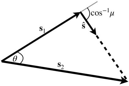
The correlation function can be computed directly as a function of (s,s1,μ)𝑠subscript𝑠1𝜇(s,s_{1},\mu), or rotated into this basis from another parametrization, for instance in terms of (s1,s2,𝐬^1𝐬^2)subscript𝑠1subscript𝑠2subscript^𝐬1subscript^𝐬2(s_{1},s_{2},\hat{\mathbf{s}}_{1}\cdot\hat{\mathbf{s}}_{2}). A pictorial representation of both coordinates system is shown in Fig. 1 We have checked that both methods give identical results, and we will use them interchangeably according to our convenience. For comparison with previous work we will more often work in the (s1,s2,𝐬^1𝐬^2)subscript𝑠1subscript𝑠2subscript^𝐬1subscript^𝐬2(s_{1},s_{2},\hat{\mathbf{s}}_{1}\cdot\hat{\mathbf{s}}_{2}) basis. The latter has the advantage of retaining a simple form even upon dropping the effective redshift approximation.
Refer to caption
Figure 1: We show the systems of coordinates adopted in this work: (s1,s2,θ)subscript𝑠1subscript𝑠2𝜃(s_{1},s_{2},\theta) and (s,s1,μ)𝑠subscript𝑠1𝜇(s,s_{1},\mu). The line of sight variables χ1subscript𝜒1\chi_{1} and χ2subscript𝜒2\chi_{2} run from the observer to the sources along the vectors 𝐬1subscript𝐬1{\bf{s}}_{1} and 𝐬2subscript𝐬2{\bf{s}}_{2}, respectively.

So far we have not assumed any theory of gravity. Now, for the rest of the manuscript we will adopt General Relativity. Therefore, by using Einstein equations to relate metric and velocity perturbations to the density fluctuation we can write the correlation function as a linear combination of the functions

In(s)=dq2π2q2P(q)j(qs)(qs)n,subscriptsuperscript𝐼𝑛𝑠d𝑞2superscript𝜋2superscript𝑞2𝑃𝑞subscript𝑗𝑞𝑠superscript𝑞𝑠𝑛I^{n}_{\ell}\left(s\right)=\int\frac{{\rm d}q}{2\pi^{2}}q^{2}P\left(q\right)\frac{j_{\ell}\left(qs\right)}{\left(qs\right)^{n}}\,, (3.7)

where P(q)𝑃𝑞P(q) is the linear matter power spectrum at z=0𝑧0z=0. In our notation, we introduce a differential operator 𝒟𝒪subscript𝒟𝒪\mathcal{D}_{\mathcal{O}} associated to each 𝒪𝒪\mathcal{O}, which allows us to arrive to

ξ𝒪𝒪(s1,s2,𝐬^1𝐬^2)subscript𝜉𝒪superscript𝒪subscript𝑠1subscript𝑠2subscript^𝐬1subscript^𝐬2\displaystyle\xi_{\mathcal{O}\mathcal{O}^{\prime}}\left(s_{1},s_{2},\hat{\bf{s}}_{1}\cdot\hat{\bf{s}}_{2}\right) (3.8)
=\displaystyle= d3q(2π)3P(q)0s1dχ10s2dχ2𝒟𝒪(q,s1,χ1)𝒟𝒪(q,s2,χ2)ei𝐪(χ2𝐬^2χ1𝐬^1)superscriptd3𝑞superscript2𝜋3𝑃𝑞superscriptsubscript0subscript𝑠1differential-dsubscript𝜒1superscriptsubscript0subscript𝑠2differential-dsubscript𝜒2subscript𝒟𝒪𝑞subscript𝑠1subscript𝜒1superscriptsubscript𝒟𝒪𝑞subscript𝑠2subscript𝜒2superscript𝑒𝑖𝐪subscript𝜒2subscript^𝐬2subscript𝜒1subscript^𝐬1\displaystyle\int\frac{{\rm d}^{3}q}{\left(2\pi\right)^{3}}P\left(q\right)\int_{0}^{s_{1}}{\rm d}\chi_{1}\int_{0}^{s_{2}}{\rm d}\chi_{2}\mathcal{D}_{\mathcal{O}}\left(q,s_{1},\chi_{1}\right)\mathcal{D}_{\mathcal{O}}^{\prime}\left(q,s_{2},\chi_{2}\right)e^{i{\bf{q}}\cdot\left(\chi_{2}\hat{\bf{s}}_{2}-\chi_{1}\hat{\bf{s}}_{1}\right)}
=\displaystyle= dq2π2q2P(q)0s1dχ10s2dχ2𝒟𝒪(q,s1,χ1)𝒟𝒪(q,s2,χ2)j0(qχ),d𝑞2superscript𝜋2superscript𝑞2𝑃𝑞superscriptsubscript0subscript𝑠1differential-dsubscript𝜒1superscriptsubscript0subscript𝑠2differential-dsubscript𝜒2subscript𝒟𝒪𝑞subscript𝑠1subscript𝜒1superscriptsubscript𝒟𝒪𝑞subscript𝑠2subscript𝜒2subscript𝑗0𝑞𝜒\displaystyle\int\frac{{\rm d}q}{2\pi^{2}}q^{2}P\left(q\right)\int_{0}^{s_{1}}{\rm d}\chi_{1}\int_{0}^{s_{2}}{\rm d}\chi_{2}\mathcal{D}_{\mathcal{O}}\left(q,s_{1},\chi_{1}\right)\mathcal{D}_{\mathcal{O}}^{\prime}\left(q,s_{2},\chi_{2}\right)j_{0}\left(q\chi\right)\,,

where χ=χ12+χ222χ1χ2cosθ𝜒superscriptsubscript𝜒12superscriptsubscript𝜒222subscript𝜒1subscript𝜒2𝜃\chi=\sqrt{\chi_{1}^{2}+\chi_{2}^{2}-2\chi_{1}\chi_{2}\cos\theta}. These differential operators, acting on j0(qχ)subscript𝑗0𝑞𝜒j_{0}\left(q\chi\right) will lead to the functions Insubscriptsuperscript𝐼𝑛I^{n}_{\ell}. To avoid confusion, in this work we will always call q𝑞q the momentum that enters the calculation of the correlation function, and k𝑘k the wavenumber associated to the actual measurement of P^L(k)subscript^𝑃𝐿𝑘\hat{P}_{L}(k). For the different perturbations we have

Dm(s1)𝒟δ=Tδ(s1)δD(s1χ1),v||(s1)𝒟v||=δD(s1χ1)TV(s1)q2χ1,v||o𝒟v||o=δD(χ1)TV(0)q2χ1,V(s1)𝒟V=δD(s1χ1)TV(s1)q2,Vo𝒟Vo=δD(χ1)TV(0)q2,Φ(s1)𝒟Φ=δD(s1χ1)TΦ(s1)q2,Ψ(s1)𝒟Ψ=δD(s1χ1)TΨ(s1)q2,Ψo𝒟Ψo=δD(χ1)Tψ(0)q2,Ψ(χ1)𝒟Ψ=TΨ(χ1)q2,Ψ˙(χ1)𝒟Ψ˙=TΨ˙(χ1)q2,Φ(χ1)𝒟Φ=TΦ(χ1)q2Φ˙(χ1)𝒟Φ˙=TΦ˙(χ1)q2.\displaystyle\begin{array}[]{cc}D_{m}\left(s_{1}\right)\rightarrow\mathcal{D}_{\delta}=T_{\delta}\left(s_{1}\right)\delta_{D}\left(s_{1}-\chi_{1}\right)\,,&\\ {v_{||}}\left(s_{1}\right)\rightarrow\mathcal{D}_{v_{||}}=\delta_{D}\left(s_{1}-\chi_{1}\right)\frac{T_{V}\left(s_{1}\right)}{q^{2}}\partial_{\chi_{1}}\,,&\hskip 14.22636pt{v_{||}}_{o}\rightarrow\mathcal{D}_{{v_{||}}_{o}}=\delta_{D}\left(\chi_{1}\right)\frac{T_{V}\left(0\right)}{q^{2}}\partial_{\chi_{1}}\,,\\ V\left(s_{1}\right)\rightarrow\mathcal{D}_{V}=\delta_{D}\left(s_{1}-\chi_{1}\right)\frac{T_{V}\left(s_{1}\right)}{q^{2}}\,,&\hskip 14.22636ptV_{o}\rightarrow\mathcal{D}_{V_{o}}=\delta_{D}\left(\chi_{1}\right)\frac{T_{V}\left(0\right)}{q^{2}}\,,\\ \Phi\left(s_{1}\right)\rightarrow\mathcal{D}_{\Phi}=\delta_{D}\left(s_{1}-\chi_{1}\right)\frac{T_{\Phi}\left(s_{1}\right)}{q^{2}}\,,&\\ \Psi\left(s_{1}\right)\rightarrow\mathcal{D}_{\Psi}=\delta_{D}\left(s_{1}-\chi_{1}\right)\frac{T_{\Psi}\left(s_{1}\right)}{q^{2}}\,,&\hskip 14.22636pt\Psi_{o}\rightarrow\mathcal{D}_{\Psi_{o}}=\delta_{D}\left(\chi_{1}\right)\frac{T_{\psi}\left(0\right)}{q^{2}}\,,\\ \Psi\left(\chi_{1}\right)\rightarrow\mathcal{D}_{\Psi}=\frac{T_{\Psi}\left(\chi_{1}\right)}{q^{2}}\,,&\hskip 14.22636pt\dot{\Psi}\left(\chi_{1}\right)\rightarrow\mathcal{D}_{\dot{\Psi}}=\frac{T_{\dot{\Psi}}\left(\chi_{1}\right)}{q^{2}}\,,\\ \Phi\left(\chi_{1}\right)\rightarrow\mathcal{D}_{\Phi}=\frac{T_{\Phi}\left(\chi_{1}\right)}{q^{2}}&\hskip 14.22636pt\dot{\Phi}\left(\chi_{1}\right)\rightarrow\mathcal{D}_{\dot{\Phi}}=\frac{T_{\dot{\Phi}}\left(\chi_{1}\right)}{q^{2}}\,.\end{array} (3.16)

Einstein gravity will constrain these transfer functions and, in particular in the absence of anisotropic stress, we have a single scalar degree of freedom. In this case the transfer functions are given by

Tδsubscript𝑇𝛿\displaystyle T_{\delta} =\displaystyle= b1D1,subscript𝑏1subscript𝐷1\displaystyle b_{1}D_{1}\,, (3.17)
TVsubscript𝑇𝑉\displaystyle T_{V} =\displaystyle= fD1,𝑓subscript𝐷1\displaystyle-\mathcal{H}fD_{1}\,, (3.18)
TΨ=TΦsubscript𝑇Ψsubscript𝑇Φ\displaystyle T_{\Psi}=T_{\Phi} =\displaystyle= 3202aΩM,0D1,32superscriptsubscript02𝑎subscriptΩ𝑀0subscript𝐷1\displaystyle-\frac{3}{2}\frac{\mathcal{H}_{0}^{2}}{a}\Omega_{M,0}D_{1}\,, (3.19)
TΨ˙=TΦ˙subscript𝑇˙Ψsubscript𝑇˙Φ\displaystyle T_{\dot{\Psi}}=T_{\dot{\Phi}} =\displaystyle= 3202aΩM,0D1(f1).32superscriptsubscript02𝑎subscriptΩ𝑀0subscript𝐷1𝑓1\displaystyle-\frac{3}{2}\frac{\mathcal{H}_{0}^{2}}{a}\Omega_{M,0}D_{1}\mathcal{H}\left(f-1\right)\,. (3.20)

where D1subscript𝐷1D_{1} is the linear growth factor and f𝑓f is the linear growth rate.

The galaxy correlation function can be computed for instance using the public code COFFE [Tansella:2018sld], which we expanded to include all possible correlations between the observer’s and source terms, between perturbations evaluated at the observer location, and to allow the multipole expansion in terms of the endpoint LOS.

The contributions arising from auto correlation of the observer terms represent the variance of these operators as they would be measured by observers with the same τosubscript𝜏𝑜\tau_{o}, i.e. they account for the difference between a randomly chosen and a preferred observer [Mitsou:2019ocs]. In the cross correlations between the observer and the source what matters are instead the fluctuations on very large scales, comparable to the distance to the source. These long wavelength modes are stochastic in nature and cannot be known a priori. For example in a determination of the observer’s velocity, what it is effectively being measured are the small scale fluctuations on the scale of our Local Group, which are by far the largest contribution to the observer’s velocity.

4 Infrared divergences of the correlation function

4.1 The variance of the galaxy density field and the 1/q41superscript𝑞41/q^{4} terms

If the expression for the galaxy number counts in Eq. (3.3) describes a gauge invariant and observable quantity, then all the summary statistics we compute out of it must be finite. However, a technical problem is immediately encountered in the calculation of the galaxy correlation functions. Namely, the contribution from any two powers of the metric potentials, for example

Φ(𝐬1)Φ(𝐬2)=0dqq22π2𝒟Φ(q,s1)𝒟Φ(q,s2)P(q)j0(qs)0dqq22π2q4P(q)j0(qs),delimited-⟨⟩Φsubscript𝐬1Φsubscript𝐬2superscriptsubscript0d𝑞superscript𝑞22superscript𝜋2subscript𝒟Φ𝑞subscript𝑠1subscript𝒟Φ𝑞subscript𝑠2𝑃𝑞subscript𝑗0𝑞𝑠proportional-tosuperscriptsubscript0d𝑞superscript𝑞22superscript𝜋2superscript𝑞4𝑃𝑞subscript𝑗0𝑞𝑠\left\langle\,\Phi({\bf{s}}_{1})\Phi({\bf{s}}_{2})\,\right\rangle=\int_{0}^{\infty}\frac{{\rm d}qq^{2}}{2\pi^{2}}\mathcal{D}_{\Phi}(q,s_{1})\mathcal{D}_{\Phi}(q,s_{2})P(q)j_{0}(qs)\propto\int_{0}^{\infty}\frac{{\rm d}qq^{2}}{2\pi^{2}}q^{-4}P(q)j_{0}(qs)\,, (4.1)

diverges in the Infra-Red (IR) for typical ΛΛ\LambdaCDM power spectra, i.e. when the lower integration limit is sent to zero. A healthy theory cannot have such a feature, which could resolve by itself within the framework, or could indicate a breakdown of one of the model assumptions.

A practical solution would be to remove by hand these divergences. This approach has been considered in [Tansella:2018sld], and we will now show that it is intimately related to the exact cancellation of the divergent terms. Consider the different operators 𝒪𝒪\cal{O} and 𝒪superscript𝒪\cal{O}^{\prime} contributing to the divergent part of the correlation function

ξdiv(s,s1,μ)𝒪𝒪ξ𝒪𝒪div(s,s1,μ)superscript𝜉div𝑠subscript𝑠1𝜇subscript𝒪superscript𝒪subscriptsuperscript𝜉div𝒪superscript𝒪𝑠subscript𝑠1𝜇\displaystyle\xi^{\rm div}(s,s_{1},\mu)\equiv\sum_{\cal{O}\cal{O}^{\prime}}\xi^{\rm div}_{\cal{O}\cal{O}^{\prime}}(s,s_{1},\mu) (4.2)

where each term is proportional to I04subscriptsuperscript𝐼40I^{4}_{0} defined in Eq. (3.7)666The different terms are proportional to I04subscriptsuperscript𝐼40I^{4}_{0} for different arguments: s𝑠s, s1subscript𝑠1s_{1}, s2subscript𝑠2s_{2}, χ1subscript𝜒1\chi_{1}, χ2subscript𝜒2\chi_{2}, s12+χ222s1χ2cosθsuperscriptsubscript𝑠12superscriptsubscript𝜒222subscript𝑠1subscript𝜒2𝜃\sqrt{s_{1}^{2}+\chi_{2}^{2}-2s_{1}\chi_{2}\cos\theta}, χ12+s222χ1s2cosθsuperscriptsubscript𝜒12superscriptsubscript𝑠222subscript𝜒1subscript𝑠2𝜃\sqrt{\chi_{1}^{2}+s_{2}^{2}-2\chi_{1}s_{2}\cos\theta} and χ12+χ222χ1χ2cosθsuperscriptsubscript𝜒12superscriptsubscript𝜒222subscript𝜒1subscript𝜒2𝜃\sqrt{\chi_{1}^{2}+\chi_{2}^{2}-2\chi_{1}\chi_{2}\cos\theta}. One way to eliminate the IR divergency is to subtract unity from the spherical Bessel function in the definition of I04subscriptsuperscript𝐼40I^{4}_{0}

I04(s)I~04(s)=dq2π2q2P(q)j0(qs)1(qs)4,subscriptsuperscript𝐼40𝑠subscriptsuperscript~𝐼40𝑠d𝑞2superscript𝜋2superscript𝑞2𝑃𝑞subscript𝑗0𝑞𝑠1superscript𝑞𝑠4I^{4}_{0}\left(s\right)\rightarrow\tilde{I}^{4}_{0}\left(s\right)=\int\frac{{\rm d}q}{2\pi^{2}}q^{2}P\left(q\right)\frac{j_{0}\left(qs\right)-1}{\left(qs\right)^{4}}\,, (4.3)

which is equivalent to removing the variance of each of the divergent pieces

ξdiv(s,s1,μ)=𝒪𝒪ξ𝒪𝒪div(s,s1,μ)=𝒪𝒪ξ~𝒪𝒪div+𝒪𝒪(σ2)𝒪𝒪div,superscript𝜉div𝑠subscript𝑠1𝜇subscript𝒪superscript𝒪subscriptsuperscript𝜉div𝒪superscript𝒪𝑠subscript𝑠1𝜇subscript𝒪superscript𝒪subscriptsuperscript~𝜉div𝒪superscript𝒪subscript𝒪superscript𝒪subscriptsuperscriptsuperscript𝜎2div𝒪superscript𝒪\xi^{\rm div}\left(s,s_{1},\mu\right)=\sum_{\cal{O}\cal{O}^{\prime}}\xi^{\rm div}_{\cal{O}\cal{O}^{\prime}}(s,s_{1},\mu)=\sum_{\cal{O}\cal{O}^{\prime}}\tilde{\xi}^{\rm div}_{\cal{O}\cal{O}^{\prime}}+\sum_{\cal{O}\cal{O}^{\prime}}(\sigma^{2})^{\rm div}_{\cal{O}\cal{O}^{\prime}}\,, (4.4)

where the new functions ξ~𝒪𝒪divsubscriptsuperscript~𝜉div𝒪superscript𝒪\tilde{\xi}^{\rm div}_{\cal{O}\cal{O}^{\prime}} are defined by the replacement of I04subscriptsuperscript𝐼40I^{4}_{0} with I~04subscriptsuperscript~𝐼40\tilde{I}^{4}_{0}. We can now compute all the ξ~~𝜉\tilde{\xi}’s, which are finite, but we are left with the problem of adding a number of infinite terms at the end. However, it turns out that the sum of the variance of the divergent pieces is identically zero,

𝒪𝒪(σ2)𝒪𝒪div=0,subscript𝒪superscript𝒪subscriptsuperscriptsuperscript𝜎2div𝒪superscript𝒪0\displaystyle\sum_{\cal{O}\cal{O}^{\prime}}(\sigma^{2})^{\rm div}_{\cal{O}\cal{O}^{\prime}}=0\,, (4.5)

once all the terms have been taken into account. Crucially the terms computed at the observer’s position are necessary for the cancellation.

This result implies that the lower integration limit in I04(s)superscriptsubscript𝐼04𝑠I_{0}^{4}(s) does not play any role once all possible correlations have been taken into account, or equivalently that the final result is not sensitive to the large scale gravitational potentials. The cancellation of the IR-divergent terms in the variance of the galaxy density field however does not imply that the observed power spectrum does not contain terms scaling like P(k)k4𝑃𝑘superscript𝑘4P(k)k^{-4}. Subtracting a constant with respect to s𝑠s as in Eq. (4.3) indeed changes only the zero mode, k=0𝑘0k=0, of PL(k)delimited-⟨⟩subscript𝑃𝐿𝑘\left\langle\,P_{L}(k)\,\right\rangle. It is straightforward to see that for any finite mode k>0𝑘0k>0, the Hankel transform of I~04superscriptsubscript~𝐼04\tilde{I}_{0}^{4} and I04superscriptsubscript𝐼04I_{0}^{4} are the same777We used dss2j0(ks)=(k>0)(k2+2kk)dsj0(ks)=(k2+2kk)π2k=0.superscript𝑘0differential-d𝑠superscript𝑠2subscript𝑗0𝑘𝑠superscriptsubscript𝑘22𝑘subscript𝑘differential-d𝑠subscript𝑗0𝑘𝑠superscriptsubscript𝑘22𝑘subscript𝑘𝜋2𝑘0\int{\rm d}ss^{2}j_{0}\left(ks\right)\stackrel{{\scriptstyle(k>0)}}{{=}}-\left(\partial_{k}^{2}+\frac{2}{k}\partial_{k}\right)\int{\rm d}sj_{0}\left(ks\right)=-\left(\partial_{k}^{2}+\frac{2}{k}\partial_{k}\right)\frac{\pi}{2k}=0\,.

4πdss2s4I~04(s)j0(ks)4𝜋differential-d𝑠superscript𝑠2superscript𝑠4subscriptsuperscript~𝐼40𝑠subscript𝑗0𝑘𝑠\displaystyle 4\pi\int{\rm d}ss^{2}s^{4}\tilde{I}^{4}_{0}\left(s\right)j_{0}\left(ks\right) =\displaystyle= 4πdss2j0(ks)dq2π2q2P(q)j0(qs)1q44𝜋differential-d𝑠superscript𝑠2subscript𝑗0𝑘𝑠d𝑞2superscript𝜋2superscript𝑞2𝑃𝑞subscript𝑗0𝑞𝑠1superscript𝑞4\displaystyle 4\pi\int{\rm d}ss^{2}j_{0}\left(ks\right)\int\frac{{\rm d}q}{2\pi^{2}}q^{2}P\left(q\right)\frac{j_{0}\left(qs\right)-1}{q^{4}} (4.6)
=\displaystyle= k2dqq2P(q)δD(qk)2πdqq2P(q)dss2j0(ks)superscript𝑘2differential-d𝑞superscript𝑞2𝑃𝑞subscript𝛿𝐷𝑞𝑘2𝜋d𝑞superscript𝑞2𝑃𝑞differential-d𝑠superscript𝑠2subscript𝑗0𝑘𝑠\displaystyle k^{-2}\int{\rm d}qq^{-2}P(q)\delta_{D}\left(q-k\right)-\frac{2}{\pi}\int\frac{{\rm d}q}{q^{2}}P\left(q\right)\int{\rm d}ss^{2}j_{0}\left(ks\right)
=(k>0)superscript𝑘0\displaystyle\stackrel{{\scriptstyle(k>0)}}{{=}} P(k)k4.𝑃𝑘superscript𝑘4\displaystyle P(k)k^{-4}\,.

We therefore conclude that the true observed power spectrum will exhibit k4P(k)superscript𝑘4𝑃𝑘k^{-4}P(k)-like behavior, which can however be exactly computed without any ad hoc procedure to tame the divergences.

The proof of Eq. (4.5) is long and tedious, and it is easily implemented with symbolic programming that can deal automatic with all the different pieces888A Mathematica notebook showing the cancellation is attached to the ArXiv submission.. It is however instructive to look at a subset of terms, specifically the ones proportional to fevosubscript𝑓evof_{\rm evo}, which cancels among themselves since fevosubscript𝑓evof_{\rm evo} is an arbitrary free parameter of the model. The derivation illustrates the physical ingredients required for the cancellations. The terms we are interested in are

Δevofevo(0Vo+ΨΨo+v||v||oV+ττo(Ψ˙+Φ˙)dτ).\Delta_{\rm evo}\equiv-f_{\rm evo}\left(\mathcal{H}_{0}V_{o}+\Psi-\Psi_{o}+{v_{||}}-{v_{||}}_{o}-\mathcal{H}V+\int_{\tau}^{\tau_{o}}\left(\dot{\Psi}+\dot{\Phi}\right){\rm d}\tau^{\prime}\right)\,. (4.7)

By using Eq. (3.16) we can compute the correlation function

ξΔevo(s1,s2,cosθ)=dq2π2q2P(q)0s1dχ10s2dχ2𝒟evo(q,s1,χ1)𝒟evo(q,s2,χ2)j0(qχ)superscript𝜉subscriptΔevosubscript𝑠1subscript𝑠2𝜃d𝑞2superscript𝜋2superscript𝑞2𝑃𝑞superscriptsubscript0subscript𝑠1differential-dsubscript𝜒1superscriptsubscript0subscript𝑠2differential-dsubscript𝜒2subscript𝒟evo𝑞subscript𝑠1subscript𝜒1subscript𝒟evo𝑞subscript𝑠2subscript𝜒2subscript𝑗0𝑞𝜒\xi^{\Delta_{\rm evo}}\left(s_{1},s_{2},\cos\theta\right)=\int\frac{{\rm d}q}{2\pi^{2}}q^{2}P\left(q\right)\int_{0}^{s_{1}}{\rm d}\chi_{1}\int_{0}^{s_{2}}{\rm d}\chi_{2}\mathcal{D}_{\rm evo}\left(q,s_{1},\chi_{1}\right)\mathcal{D}_{\rm evo}\left(q,s_{2},\chi_{2}\right)j_{0}\left(q\chi\right) (4.8)

where 𝒟evosubscript𝒟evo\mathcal{D}_{\rm evo} is the differential operator associated to Eq. (4.7), through the mapping in Eq. (3.16). In order to show that IR divergent contributions to the variance vanish we need to check that

limq0q40s1dχ10s2dχ2𝒟evo(q,s1,χ1)𝒟evo(q,s2,χ2)j0(qχ)=0.subscript𝑞0superscript𝑞4superscriptsubscript0subscript𝑠1differential-dsubscript𝜒1superscriptsubscript0subscript𝑠2differential-dsubscript𝜒2subscript𝒟evo𝑞subscript𝑠1subscript𝜒1subscript𝒟evo𝑞subscript𝑠2subscript𝜒2subscript𝑗0𝑞𝜒0\lim_{q\rightarrow 0}q^{4}\int_{0}^{s_{1}}{\rm d}\chi_{1}\int_{0}^{s_{2}}{\rm d}\chi_{2}\mathcal{D}_{\rm evo}\left(q,s_{1},\chi_{1}\right)\mathcal{D}_{\rm evo}\left(q,s_{2},\chi_{2}\right)j_{0}\left(q\chi\right)=0\,. (4.9)

A little algebra shows that this condition is satisfied only if

0s1dχ1(TΨ˙(χ1)+TΦ˙(χ1))(s1)TV(s1)+0TV(0)+TΨ(s1)TΨ(0)=0,superscriptsubscript0subscript𝑠1differential-dsubscript𝜒1subscript𝑇˙Ψsubscript𝜒1subscript𝑇˙Φsubscript𝜒1subscript𝑠1subscript𝑇𝑉subscript𝑠1subscript0subscript𝑇𝑉0subscript𝑇Ψsubscript𝑠1subscript𝑇Ψ00\int_{0}^{s_{1}}{\rm d}\chi_{1}\left(T_{\dot{\Psi}}(\chi_{1})+T_{\dot{\Phi}}(\chi_{1})\right)-\mathcal{H}(s_{1})T_{V}(s_{1})+\mathcal{H}_{0}T_{V}(0)+T_{\Psi}(s_{1})-T_{\Psi}(0)=0\,, (4.10)

which by integrating over χ1subscript𝜒1\chi_{1} reduces to

TΦ(s1)+(s1)TV(s1)=TΦ(0)+0TV(0)=constant.subscript𝑇Φsubscript𝑠1subscript𝑠1subscript𝑇𝑉subscript𝑠1subscript𝑇Φ0subscript0subscript𝑇𝑉0constantT_{\Phi}\left(s_{1}\right)+\mathcal{H}\left(s_{1}\right)T_{V}\left(s_{1}\right)=T_{\Phi}\left(0\right)+\mathcal{H}_{0}T_{V}\left(0\right)={\rm constant}\,. (4.11)

In terms of the metric perturbation and the peculiar velocity this condition reads

Φ(k,τ)+(τ)kv(k,τ)=constantfor k0.formulae-sequenceΦ𝑘𝜏𝜏𝑘𝑣𝑘𝜏constantfor 𝑘0\Phi\left(k,\tau\right)+\frac{\mathcal{H}\left(\tau\right)}{k}v\left(k,\tau\right)={\rm constant}\qquad\text{for }\quad k\rightarrow 0\,. (4.12)

It is easy to show that this condition is satisfied by the Weinberg adiabatic mode [Weinberg:2003sw], under the assumption that dark matter is the only clustering species. The existence of such adiabatic mode indeed guarantees that the long wavelength gravitational potential is unobservable and can always be reabsorbed with a change of coordinates. In this case for the dark matter velocity we have

vM=kΦ˙+Φ4πGa2ρ¯M=kΦ˙+Φ23˙,subscript𝑣𝑀𝑘˙ΦΦ4𝜋𝐺superscript𝑎2subscript¯𝜌𝑀𝑘˙ΦΦsuperscript23˙v_{M}=k\frac{\dot{\Phi}+\mathcal{H}\Phi}{4\pi Ga^{2}\bar{\rho}_{M}}=k\frac{\dot{\Phi}+\mathcal{H}\Phi}{\mathcal{H}^{2}-3\dot{\mathcal{H}}}\,, (4.13)

where we have explicitly used Φ=ΨΦΨ\Phi=\Psi. Then by plugging this expression into Eq. (4.12) and taking a time derivative we obtain a second order differential equation for ΦΦ\Phi

Φ¨+3Φ˙+(2+2˙)Φ=0,¨Φ3˙Φsuperscript22˙Φ0\ddot{\Phi}+3\mathcal{H}\dot{\Phi}+\left(\mathcal{H}^{2}+2\dot{\mathcal{H}}\right)\Phi=0\,, (4.14)

where we have used

a˙˙˙=2a2(2aa˙a¨a˙3).˙˙˙𝑎2superscript𝑎22𝑎˙𝑎¨𝑎superscript˙𝑎3\dddot{a}=\frac{2}{a^{2}}\left(2a\dot{a}\ddot{a}-\dot{a}^{3}\right)\,. (4.15)

The differential equation in Eq. (4.14) is precisely solved by the Weinberg adiabatic mode999In Eq. (4.16) we have neglected the decaying mode. [Weinberg:2003sw, Mirbabayi:2014hda]

Ψ=Φ=C1(a20τa2𝑑τ1).ΨΦsubscript𝐶1superscript𝑎2superscriptsubscript0𝜏superscript𝑎2differential-dsuperscript𝜏1\Psi=\Phi=C_{1}\left(\frac{\mathcal{H}}{a^{2}}\int_{0}^{\tau}a^{2}d\tau^{\prime}-1\right)\,. (4.16)

Therefore we conclude that cancellation of the IR divergences is a direct consequence of the existence of the Weinberg adiabatic mode as a solution of the Einstein field equations. We also recognize that Eq. (4.12) agrees with the spatial curvature perturbation on co-moving spatial surface

co(k,τ)=Φ(k,τ)+(τ)kv(k,τ)subscript𝑐𝑜𝑘𝜏Φ𝑘𝜏𝜏𝑘𝑣𝑘𝜏-\mathcal{R}_{co}\left(k,\tau\right)=\Phi\left(k,\tau\right)+\frac{\mathcal{H}\left(\tau\right)}{k}v\left(k,\tau\right) (4.17)

which is conserved on super-Hubble scales for adiabatic perturbations in absence of anisotropic stresses.

In presence of local Primordial Non Gaussianities, the sensitivity of the two-point function to the long-wavelength gravitational potential is physical, and it cannot therefore be removed. In this case, the correlation between large and small scale modes is actually imprinted during inflation. On the other hand, it is possible to show that the IR divergences are solely due to the auto-correlation of the primordial gravitational potential, and are hence proportional to fNL2superscriptsubscript𝑓NL2f_{\rm NL}^{2}. The terms involving one power of fNLsubscript𝑓NLf_{\rm NL} and a metric perturbation are all individually divergent in the IR, but once again their sum is finite. This result is a consequence of the fact that in the squeezed limit local PNG cannot be generated by gravitational evolution.

Finally we notice that from the expression derived in this section, Eq. (4.9), directly implies

limq0q30s1dχ10s2dχ2𝒟evo(q,s1,χ1)𝒟evo(q,s2,χ2)j0(qχ)=0.subscript𝑞0superscript𝑞3superscriptsubscript0subscript𝑠1differential-dsubscript𝜒1superscriptsubscript0subscript𝑠2differential-dsubscript𝜒2subscript𝒟evo𝑞subscript𝑠1subscript𝜒1subscript𝒟evo𝑞subscript𝑠2subscript𝜒2subscript𝑗0𝑞𝜒0\lim_{q\rightarrow 0}q^{3}\int_{0}^{s_{1}}{\rm d}\chi_{1}\int_{0}^{s_{2}}{\rm d}\chi_{2}\mathcal{D}_{\rm evo}\left(q,s_{1},\chi_{1}\right)\mathcal{D}_{\rm evo}\left(q,s_{2},\chi_{2}\right)j_{0}\left(q\chi\right)=0\,. (4.18)

4.2 The 1/q21superscript𝑞21/q^{2} IR sensitivity

The terms involving one power of the metric potentials are not IR sensitive in a ΛΛ\LambdaCDM Universe with parameters as determined by the Planck satellite [Aghanim:2018eyx]. Nevertheless, in the limit q0𝑞0q\rightarrow 0 we expect the gravitational potentials to disappear from the correlation function as shown in the previous section. This is an important consistency check of the theory, because, if the cancellation is a property of General Relativity and of Gaussian and adiabatic initial conditions, then long-wavelength modes are unobservable regardless of the actual value of cosmological parameters. Following the example in the previous section we show this is the case for the contribution in Eq. (4.7), while a complete treatment can be easily obtained through symbolic programming.

Inspection of Eq. (4.7), reveals that we need to consider two set of terms to show the cancellation of a single metric potential in the large scale limit. Indeed we do not only have the contribution induced by the peculiar velocities, i.e. proportional to the gradient of the gravitational potential, but also the terms proportional to two powers of the gravitational potential combined with the expansion of the spherical Bessel at the order q2superscript𝑞2q^{2}. In terms of the transfer function TΨsubscript𝑇ΨT_{\Psi}, TΨ˙subscript𝑇˙ΨT_{\dot{\Psi}} and TVsubscript𝑇𝑉T_{V} we arrive to

limq0q20s1dχ10s2dχ2𝒟evo(q,s1,χ1)𝒟evo(q,s2,χ2)j0(qχ)subscript𝑞0superscript𝑞2superscriptsubscript0subscript𝑠1differential-dsubscript𝜒1superscriptsubscript0subscript𝑠2differential-dsubscript𝜒2subscript𝒟evo𝑞subscript𝑠1subscript𝜒1subscript𝒟evo𝑞subscript𝑠2subscript𝜒2subscript𝑗0𝑞𝜒\displaystyle\lim_{q\rightarrow 0}q^{2}\int_{0}^{s_{1}}{\rm d}\chi_{1}\int_{0}^{s_{2}}{\rm d}\chi_{2}\mathcal{D}_{\rm evo}\left(q,s_{1},\chi_{1}\right)\mathcal{D}_{\rm evo}\left(q,s_{2},\chi_{2}\right)j_{0}\left(q\chi\right) (4.19)
=\displaystyle= (s1s2)1160s1dχ10s2dχ2superscriptsubscript𝑠1subscript𝑠2116superscriptsubscript0subscript𝑠1differential-dsubscript𝜒1superscriptsubscript0subscript𝑠2differential-dsubscript𝜒2\displaystyle\left(s_{1}s_{2}\right)^{-1}\frac{1}{6}\int_{0}^{s_{1}}{\rm d}\chi_{1}\int_{0}^{s_{2}}{\rm d}\chi_{2}
{2χ12s1TΨ˙(χ1)(TΨ(0)0TV(0))4Δχ2s1s2TΨ˙(χ1)TΨ˙(χ2)\displaystyle\left\{2\chi_{1}^{2}s_{1}T_{\dot{\Psi}}(\chi_{1})(T_{\Psi}(0)-\mathcal{H}_{0}T_{V}(0))-4\Delta\chi^{2}s_{1}s_{2}T_{\dot{\Psi}}(\chi_{1})T_{\dot{\Psi}}(\chi_{2})\right.
+4s1TΨ˙(χ1)TV(s2)(χ1ys2)4χ1ys1TV(0)TΨ˙(χ1)4subscript𝑠1subscript𝑇˙Ψsubscript𝜒1subscript𝑇𝑉subscript𝑠2subscript𝜒1𝑦subscript𝑠24subscript𝜒1𝑦subscript𝑠1subscript𝑇𝑉0subscript𝑇˙Ψsubscript𝜒1\displaystyle+4s_{1}T_{\dot{\Psi}}(\chi_{1})T_{V}(s_{2})(\chi_{1}y-s_{2})-4\chi_{1}ys_{1}T_{V}(0)T_{\dot{\Psi}}(\chi_{1})
2Δχ12s1TΨ˙(χ1)(TΨ(s2)(s2)TV(s2))2Δsuperscriptsubscript𝜒12subscript𝑠1subscript𝑇˙Ψsubscript𝜒1subscript𝑇Ψsubscript𝑠2subscript𝑠2subscript𝑇𝑉subscript𝑠2\displaystyle-2\Delta\chi_{1}^{2}s_{1}T_{\dot{\Psi}}(\chi_{1})(T_{\Psi}(s_{2})-\mathcal{H}(s_{2})T_{V}(s_{2}))
+2χ22s2TΨ˙(χ2)(TΨ(0)0TV(0))2superscriptsubscript𝜒22subscript𝑠2subscript𝑇˙Ψsubscript𝜒2subscript𝑇Ψ0subscript0subscript𝑇𝑉0\displaystyle+2\chi_{2}^{2}s_{2}T_{\dot{\Psi}}(\chi_{2})(T_{\Psi}(0)-\mathcal{H}_{0}T_{V}(0))
+4s2TΨ˙(χ2)TV(s1)(χ2ys1)4χ2ys2TV(0)TΨ˙(χ2)4subscript𝑠2subscript𝑇˙Ψsubscript𝜒2subscript𝑇𝑉subscript𝑠1subscript𝜒2𝑦subscript𝑠14subscript𝜒2𝑦subscript𝑠2subscript𝑇𝑉0subscript𝑇˙Ψsubscript𝜒2\displaystyle+4s_{2}T_{\dot{\Psi}}(\chi_{2})T_{V}(s_{1})(\chi_{2}y-s_{1})-4\chi_{2}ys_{2}T_{V}(0)T_{\dot{\Psi}}(\chi_{2})
2Δχ22s2TΨ˙(χ2)(TΨ(s1)(s1)TV(s1))2Δsuperscriptsubscript𝜒22subscript𝑠2subscript𝑇˙Ψsubscript𝜒2subscript𝑇Ψsubscript𝑠1subscript𝑠1subscript𝑇𝑉subscript𝑠1\displaystyle-2\Delta\chi_{2}^{2}s_{2}T_{\dot{\Psi}}(\chi_{2})(T_{\Psi}(s_{1})-\mathcal{H}(s_{1})T_{V}(s_{1}))
+2TV(s1)(ys1TV(0)(s1)TV(0)(y+0s1)+s1TΨ(0))2subscript𝑇𝑉subscript𝑠1𝑦subscript𝑠1subscript𝑇𝑉0subscript𝑠1subscript𝑇𝑉0𝑦subscript0subscript𝑠1subscript𝑠1subscript𝑇Ψ0\displaystyle+2T_{V}(s_{1})(ys_{1}T_{V}(0)\mathcal{H}(s_{1})-T_{V}(0)(y+\mathcal{H}_{0}s_{1})+s_{1}T_{\Psi}(0))
+2TV(s2)(ys2TV(0)(s2)TV(0)(y+0s2)+s2TΨ(0))2subscript𝑇𝑉subscript𝑠2𝑦subscript𝑠2subscript𝑇𝑉0subscript𝑠2subscript𝑇𝑉0𝑦subscript0subscript𝑠2subscript𝑠2subscript𝑇Ψ0\displaystyle+2T_{V}(s_{2})(ys_{2}T_{V}(0)\mathcal{H}(s_{2})-T_{V}(0)(y+\mathcal{H}_{0}s_{2})+s_{2}T_{\Psi}(0))
+2TV(s2)(TV(s1)((s1)(s2ys1)+(s2)(s1ys2)+y)\displaystyle+2T_{V}(s_{2})(T_{V}(s_{1})(\mathcal{H}(s_{1})(s_{2}-ys_{1})+\mathcal{H}(s_{2})(s_{1}-ys_{2})+y)
+TΨ(s1)(ys1s2))2TV(s1)TΨ(s2)(s1ys2)\displaystyle+T_{\Psi}(s_{1})(ys_{1}-s_{2}))-2T_{V}(s_{1})T_{\Psi}(s_{2})(s_{1}-ys_{2})
2ys1TV(0)TΨ(s1)2ys2TV(0)TΨ(s2)+2yTV(0)22𝑦subscript𝑠1subscript𝑇𝑉0subscript𝑇Ψsubscript𝑠12𝑦subscript𝑠2subscript𝑇𝑉0subscript𝑇Ψsubscript𝑠22𝑦subscript𝑇𝑉superscript02\displaystyle-2ys_{1}T_{V}(0)T_{\Psi}(s_{1})-2ys_{2}T_{V}(0)T_{\Psi}(s_{2})+2yT_{V}(0)^{2}
+s12(TΨ(0)0TV(0))(TΨ(s1)(s1)TV(s1))superscriptsubscript𝑠12subscript𝑇Ψ0subscript0subscript𝑇𝑉0subscript𝑇Ψsubscript𝑠1subscript𝑠1subscript𝑇𝑉subscript𝑠1\displaystyle+s_{1}^{2}(T_{\Psi}(0)-\mathcal{H}_{0}T_{V}(0))(T_{\Psi}(s_{1})-\mathcal{H}(s_{1})T_{V}(s_{1}))
+s22(TΨ(0)0TV(0))(TΨ(s2)(s2)TV(s2))superscriptsubscript𝑠22subscript𝑇Ψ0subscript0subscript𝑇𝑉0subscript𝑇Ψsubscript𝑠2subscript𝑠2subscript𝑇𝑉subscript𝑠2\displaystyle+s_{2}^{2}(T_{\Psi}(0)-\mathcal{H}_{0}T_{V}(0))(T_{\Psi}(s_{2})-\mathcal{H}(s_{2})T_{V}(s_{2}))
s2(TΨ(s1)(s1)TV(s1))(TΨ(s2)(s2)TV(s2))},\displaystyle\left.-s^{2}(T_{\Psi}(s_{1})-\mathcal{H}(s_{1})T_{V}(s_{1}))(T_{\Psi}(s_{2})-\mathcal{H}(s_{2})T_{V}(s_{2}))\right\}\,,

where we have introduced y=cosθ𝑦𝜃y=\cos\theta. Now combining the Euler equation

T˙V+TV=TΨsubscript˙𝑇𝑉subscript𝑇𝑉subscript𝑇Ψ\dot{T}_{V}+\mathcal{H}T_{V}=T_{\Psi} (4.20)

and the condition in Eq. (4.12), which we remind is satisfied Weinberg the adiabatic mode, we obtain

TΨ=12(TΨ(0)+0TV(0)+T˙V)subscript𝑇Ψ12subscript𝑇Ψ0subscript0subscript𝑇𝑉0subscript˙𝑇𝑉T_{\Psi}=\frac{1}{2}\left(T_{\Psi}\left(0\right)+\mathcal{H}_{0}T_{V}\left(0\right)+\dot{T}_{V}\right) (4.21)

or equivalently

0s1dχ1TΨ(χ1)=s12[TΨ(0)+0TV(0)+12(TV(0)TV(s1))].superscriptsubscript0subscript𝑠1differential-dsubscript𝜒1subscript𝑇Ψsubscript𝜒1subscript𝑠12delimited-[]subscript𝑇Ψ0subscript0subscript𝑇𝑉012subscript𝑇𝑉0subscript𝑇𝑉subscript𝑠1\int_{0}^{s_{1}}{\rm d}\chi_{1}T_{\Psi}\left(\chi_{1}\right)=\frac{s_{1}}{2}\left[T_{\Psi}\left(0\right)+\mathcal{H}_{0}T_{V}\left(0\right)+\frac{1}{2}\left(T_{V}\left(0\right)-T_{V}\left(s_{1}\right)\right)\right]\,. (4.22)

After some integration by parts and using the Friedman Equation ˙=2302ΩM02a˙superscript23superscriptsubscript02subscriptΩ𝑀02𝑎\dot{\mathcal{H}}=\mathcal{H}^{2}-\frac{3\mathcal{H}_{0}^{2}\Omega_{M0}}{2a}, we obtain the desired cancellation

limq0q20s1dχ10s2dχ2𝒟evo(q,s1,χ1)𝒟evo(q,s2,χ2)j0(qχ)=0,subscript𝑞0superscript𝑞2superscriptsubscript0subscript𝑠1differential-dsubscript𝜒1superscriptsubscript0subscript𝑠2differential-dsubscript𝜒2subscript𝒟evo𝑞subscript𝑠1subscript𝜒1subscript𝒟evo𝑞subscript𝑠2subscript𝜒2subscript𝑗0𝑞𝜒0\lim_{q\rightarrow 0}q^{2}\int_{0}^{s_{1}}{\rm d}\chi_{1}\int_{0}^{s_{2}}{\rm d}\chi_{2}\mathcal{D}_{\rm evo}\left(q,s_{1},\chi_{1}\right)\mathcal{D}_{\rm evo}\left(q,s_{2},\chi_{2}\right)j_{0}\left(q\chi\right)=0\,, (4.23)

and as a consequence also that

limq0q0s1dχ10s2dχ2𝒟evo(q,s1,χ1)𝒟evo(q,s2,χ2)j0(qχ)=0.subscript𝑞0𝑞superscriptsubscript0subscript𝑠1differential-dsubscript𝜒1superscriptsubscript0subscript𝑠2differential-dsubscript𝜒2subscript𝒟evo𝑞subscript𝑠1subscript𝜒1subscript𝒟evo𝑞subscript𝑠2subscript𝜒2subscript𝑗0𝑞𝜒0\lim_{q\rightarrow 0}q\int_{0}^{s_{1}}{\rm d}\chi_{1}\int_{0}^{s_{2}}{\rm d}\chi_{2}\mathcal{D}_{\rm evo}\left(q,s_{1},\chi_{1}\right)\mathcal{D}_{\rm evo}\left(q,s_{2},\chi_{2}\right)j_{0}\left(q\chi\right)=0\,. (4.24)

Similarly to the discussion of the divergent terms in the previous section, the cancellation only affects the zero mode of the power spectrum, hence GR contributions proportional to P(k)k2𝑃𝑘superscript𝑘2P(k)k^{-2} are present at any finite scale.

To summarise this Section, we found that the existence of the Weinberg adiabatic mode removes the IR sensitivity of the correlation function. The presence of the adiabatic mode is guaranteed for Gaussian and adiabatic initial conditions and by the diffeomorphism invariance of General Relativity. Notice all three conditions are required. We already discussed how local PNG induce correlation between long and short wavelength modes. If the initial conditions contained some amount of isocuvature perturbations or new long range forces are present in the dark sector, then the comoving curvature perturbation is not constant on super-horizon scales and the correlation function could exhibit a weak IR dependence.

While our calculation addresses the specific problem of the computation of the galaxy correlation function and power spectrum, similar arguments about the effects of long wavelength gravitational potentials, or better said lack thereof, on cosmological observables have long been known. For the late Universe, they usually exploit the Consistency Relations for LSS [Creminelli2013, Peloso2013, Kehagias2013], which are valid under the same conditions required by the cancellation we showed above. For an application of the Consistency Relations to the relativistic bispectrum see [Kehagias:2015tda]. Our result also implies that GR effects are not coupled to any super sample value of the gravitational potential and its spatial derivative, as it would be the case in presence of local PNG [Castorina2020].

Our findings are in disagreement with the recent work in [Grimm:2020ays]. They assume that the observed power spectrum constructed from squaring the Fourier transform of the galaxy overdensity field is diagonal, i.e. the field is homogeneous and isotropic. But as we discussed in the introduction, RSD and GR effects break translational and rotational invariance: the Yamamoto estimator is a function of a single k𝑘k mode because the other one has been integrated out. The power spectrum discussed in [Grimm:2020ays] is therefore not directly related to any observable. Where we agree with [Grimm:2020ays] is in the calculation of the variance of the galaxy overdensity field, which does not receive contribution from the gravitational potential and its first derivatives. As discussed above we clarified the necessary physical conditions for this cancellation, which requires more than just the equivalence principle to hold as suggested by [Grimm:2020ays]. The full two-point correlation function of the galaxy density field and any general estimator for the power spectrum like the one Eq. (2.1), are complicated average of all possible lines of sight for each pair of galaxies and should not be compared with the variance of the field itself, which is a function of a single line of sight.

Finally, one could argue that the any IR sensitivity of the model adopted here would be anyway removed by the presence of an Integral Constraint (IC). This could be the case, however it is important to check that the relativistic expression for the galaxy number counts provide a finite answer regardless of the way the mean number density of galaxy is measured. If one wants to resort to the IC, the latter should be included at the level of the integrand in Eq. (2.1), carefully including the effect of the window function. In our approach we removed the IR sensitivity in both Eq. (2.1) and in the expression of the IC, which can be therefore discarded for most practical applications.

The method described in this work to remove the IR divergences is also the only one that can deal with observations in which the mean is not known or cannot be measured. This is for instance the case of the excess brightness temperature of the 21 cm line, or any intensity line, measured with radio arrays in interefometric mode. With interferometers we directly have access to the fluctuations in Fourier Space, and there is no IC to subtract to the measurements of the power spectrum.

5 Relativistic effects in the galaxy power spectrum

Having resolved the issue of IR divergences in the correlation function we can now safely proceed to compute the prediction for the observed galaxy power spectrum multipoles. Our calculation of the correlation function includes the observer’s terms, in auto-correlation with themselves and in cross-correlations with the source terms. Given the gauge invariant galaxy number counts, Eq. (3.3), we still have the freedom to perform a Lorentz boost to a preferred reference frame. In particular we are allowed to move to the CMB rest frame, and remove the terms proportional to the observer’s velocity. While this operation is harmless in the theoretical prediction, some care should be used when expressing the measurement in the CMB or any other frame [Kaiser:1987qv, Hamilton:1997zq]. Alternatively one can keep these terms and try to measure the induced dipole to test the Copernican Principle. We provide expressions for this case in Appendix C.

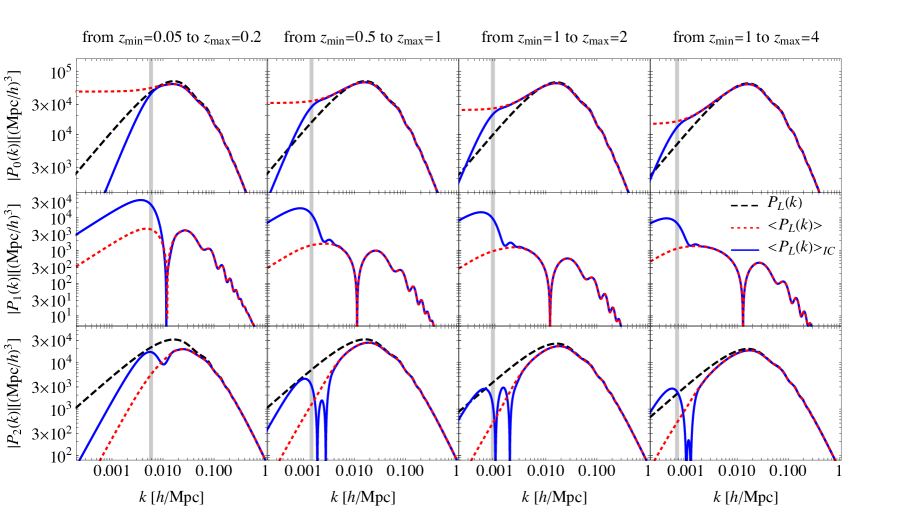
The other required model ingredients are the multipoles of the window functions F(s,s1)subscript𝐹𝑠subscript𝑠1F_{\ell}(s,s_{1}), and the Fourier space windows functions QL(k)subscript𝑄𝐿𝑘Q_{L}(k). While our expressions are fully general, we choose a rather simple survey geometry, whose properties can be analytically calculated. We thus assume that the window function has an azimuthal symmetry around an axes, for instance a spherical cap with a maximum opening angle θmaxsubscript𝜃max\theta_{\rm max}. We fix this angle by imposing the hypothetical survey covers one third of the sky, fsky=1/3subscript𝑓sky13f_{\rm sky}=1/3. This assumption allows us to sum over all values of \ell and 1subscript1\ell_{1} in Eq. (2.1). We also assume that the radial selection function and angular footprint can be separated, which might not always be the case if different parts of the sky have large depth variations. Finally we assume a constant selection functions within a certain redshift range. We consider four redshift bins, [zmin=0.05,zmax=0.2]delimited-[]formulae-sequencesubscript𝑧min0.05subscript𝑧max0.2[z_{\rm min}=0.05,z_{\rm max}=0.2], [0.5,1], [1,2] and [1,4]. For these choices of window function, the convolution with the correlation function further simplifies, as discussed in Appendix A. Figure 2 shows the multipoles QL(s)subscript𝑄𝐿𝑠Q_{L}(s) and QL(k)subscript𝑄𝐿𝑘Q_{L}(k) in our four reference surveys, for L=0,1,2𝐿012L=0,1,2. The largest pair separation for an azimuthally symmetric survey geometry is given by 2r(zmax)sinθmax2𝑟subscript𝑧maxsubscript𝜃max2r(z_{\rm max})\sin\theta_{\rm max}, where θmax=cos1(12fsky)subscript𝜃maxsuperscript112subscript𝑓sky\theta_{\rm max}=\cos^{-1}\left(1-2f_{\rm sky}\right). We see that the scale k2π/(2r(zmax)sinθmax)similar-to𝑘2𝜋2𝑟subscript𝑧maxsubscript𝜃maxk\sim 2\pi/\left(2r(z_{\rm max})\sin\theta_{\rm max}\right) indicates the boundary of the survey volume in Fourier space and we will display it in the other figures as well. The effect of the window function is quite dramatic at low k𝑘k, as one can see in Fig. 3. The black dashed lines show the flat-sky prediction for the multipoles of the power spectrum without the window function, while the blue and red ones display the convolution with the window function, with and without the Integral Constraint respectively. Notice that our asymmetric choice of LOS generates a power spectrum dipole, as shown in the second row of Fig. 3.

Refer to caption
Refer to caption
Figure 2: We show the multipoles of the window functions considered in the manuscript QL(s)subscript𝑄𝐿𝑠Q_{L}\left(s\right) and its Hankel transforms QL(k)subscript𝑄𝐿𝑘Q_{L}\left(k\right) for the monopole (L=0𝐿0L=0), the dipole (L=1𝐿1L=1) and the quadrupole (L=2𝐿2L=2), normalized to Q0(k0)=1subscript𝑄0𝑘01Q_{0}\left(k\rightarrow 0\right)=1. The window function is defined as ϕ(𝐬1)=ϕ(s1)W(𝐬^1)=Θ(s1smin)Θ(smaxs1)Θ(θmaxθ1)italic-ϕsubscript𝐬1italic-ϕsubscript𝑠1𝑊subscript^𝐬1Θsubscript𝑠1subscript𝑠minΘsubscript𝑠maxsubscript𝑠1Θsubscript𝜃maxsubscript𝜃1\phi\left({\bf{s}}_{1}\right)=\phi\left(s_{1}\right)W\left(\hat{\bf{s}}_{1}\right)=\Theta\left(s_{1}-s_{\rm min}\right)\Theta\left(s_{\rm max}-s_{1}\right)\Theta\left(\theta_{\rm max}-\theta_{1}\right), where θmax=cos1(12fsky)subscript𝜃maxsuperscript112subscript𝑓sky\theta_{\rm max}=\cos^{-1}\left(1-2f_{\rm sky}\right) and we set fsky=1/3subscript𝑓sky13f_{\rm sky}=1/3. The vertical lines correspond to the largest scales probed by the survey, i.e. 2r(zmax)sinθmax2𝑟subscript𝑧maxsubscript𝜃max2r(z_{\rm max})\sin\theta_{\rm max} in real space and 2π/(2r(zmax)sinθmax)2𝜋2𝑟subscript𝑧maxsubscript𝜃max2\pi/\left(2r(z_{\rm max})\sin\theta_{\rm max}\right) in Fourier space.

5.1 Density and RSD

In the small angle limit the standard density and RSD correlation function and power spectrum correspond to the plane parallel limit of Kaiser [Kaiser:1987qv]. For wide area surveys, like DESI or Euclid, deviations from the plane parallel regime take the name of wide-angle effects. The amplitude of these terms is controlled by kseff𝑘subscript𝑠effks_{\rm eff}, where seffsubscript𝑠effs_{\rm eff} is the comoving distance to the effective redshift, as opposed to k/𝑘k/\cal{H} for the other relativistic effects. Therefore for surveys of the size of the Hubble horizon, seff1similar-tosubscript𝑠effsuperscript1s_{\rm eff}\sim\mathcal{H}^{-1}, these effects are comparable, while for smaller surveys wide-angle effects are more important.

To derive the correlation function induced by density and redshift perturbations, i.e. what we denote by the standard Newtonian contribution to galaxy clustering, we follow Eq. (3.8),

ξnewt(s1,s2,𝐬^1𝐬^2)=(b1Dm+1rv||)(𝐬1)(b1Dm+1rv||)(𝐬2)=\displaystyle\xi^{\rm newt}\left(s_{1},s_{2},\hat{\bf{s}}_{1}\cdot\hat{\bf{s}}_{2}\right)=\langle\left(b_{1}D_{m}+\mathcal{H}^{-1}\partial_{r}{v_{||}}\right)\left({\bf{s}}_{1}\right)\left(b_{1}D_{m}+\mathcal{H}^{-1}\partial_{r}{v_{||}}\right)\left({\bf{s}}_{2}\right)\rangle= (5.1)
=\displaystyle= dq2π2q2P(q)D1(s1)D1(s2)(b1(s1)f(s1)qs12)(b1(s2)f(s2)qs22)j0(qs)d𝑞2superscript𝜋2superscript𝑞2𝑃𝑞subscript𝐷1subscript𝑠1subscript𝐷1subscript𝑠2subscript𝑏1subscript𝑠1𝑓subscript𝑠1subscriptsuperscript2𝑞subscript𝑠1subscript𝑏1subscript𝑠2𝑓subscript𝑠2subscriptsuperscript2𝑞subscript𝑠2subscript𝑗0𝑞𝑠\displaystyle\int\frac{{\rm d}q}{2\pi^{2}}q^{2}P\left(q\right)D_{1}\left(s_{1}\right)D_{1}\left(s_{2}\right)\left(b_{1}\left(s_{1}\right)-f\left(s_{1}\right)\partial^{2}_{qs_{1}}\right)\left(b_{1}\left(s_{2}\right)-f\left(s_{2}\right)\partial^{2}_{qs_{2}}\right)j_{0}\left(qs\right)
=\displaystyle= i=0,2,4Ji(s1,s2,cosθ)Ii0(s)D1(s1)D1(s2),subscript𝑖024subscript𝐽𝑖subscript𝑠1subscript𝑠2𝜃subscriptsuperscript𝐼0𝑖𝑠subscript𝐷1subscript𝑠1subscript𝐷1subscript𝑠2\displaystyle\sum_{i=0,2,4}J_{i}\left(s_{1},s_{2},\cos\theta\right)I^{0}_{i}\left(s\right)D_{1}\left(s_{1}\right)D_{1}\left(s_{2}\right)\,,

where

J0(s1,s2,cosθ)subscript𝐽0subscript𝑠1subscript𝑠2𝜃\displaystyle J_{0}\left(s_{1},s_{2},\cos\theta\right) =\displaystyle= 115(f(s1)(5b1(s2)+2cos2θf(s2)+f(s2))+5b1(s1)(3b1(s2)+f(s2))),115𝑓subscript𝑠15subscript𝑏1subscript𝑠22superscript2𝜃𝑓subscript𝑠2𝑓subscript𝑠25subscript𝑏1subscript𝑠13subscript𝑏1subscript𝑠2𝑓subscript𝑠2\displaystyle\frac{1}{15}\left(f(s_{1})\left(5b_{1}(s_{2})+2{\cos^{2}\theta}f(s_{2})+f(s_{2})\right)+5b_{1}(s_{1})(3b_{1}(s_{2})+f(s_{2}))\right)\,,
J2(s1,s2,cosθ)subscript𝐽2subscript𝑠1subscript𝑠2𝜃\displaystyle J_{2}\left(s_{1},s_{2},\cos\theta\right) =\displaystyle= 121s2{(7b1(s2)f(s1)((3cos2θ1)s224cosθs1s2+2s12)\displaystyle-\frac{1}{21s^{2}}\left\{\left(7b_{1}(s_{2})f(s_{1})\left(\left(3{\cos^{2}\theta}-1\right)s_{2}^{2}-4{\cos\theta}s_{1}s_{2}+2s_{1}^{2}\right)\right.\right. (5.3)
+f(s2)(7b1(s1)((3cos2θ1)s124cosθs1s2+2s22)\displaystyle+f(s_{2})\left(7b_{1}(s_{1})\left(\left(3{\cos^{2}\theta}-1\right)s_{1}^{2}-4{\cos\theta}s_{1}s_{2}+2s_{2}^{2}\right)\right.
+f(s1)((11cos2θ+1)s124cosθ(cos2θ+5)s1s2\displaystyle\left.\left.\left.+f(s_{1})\left(\left(11{\cos^{2}\theta}+1\right)s_{1}^{2}-4{\cos\theta}\left({\cos^{2}\theta}+5\right)s_{1}s_{2}\right.\right.\right.\right.
+(11cos2θ+1)s22)))},\displaystyle\left.\left.\left.\left.\qquad\qquad+\left(11{\cos^{2}\theta}+1\right)s_{2}^{2}\right)\right)\right)\right\}\,,
J4(s1,s2,cosθ)subscript𝐽4subscript𝑠1subscript𝑠2𝜃\displaystyle J_{4}\left(s_{1},s_{2},\cos\theta\right) =\displaystyle= f(s1)f(s2)560s4s12s22{4(30cos2θ19)s16s228cosθ(4cos2θ+39)s15s23\displaystyle\frac{f(s_{1})f(s_{2})}{560s^{4}s_{1}^{2}s_{2}^{2}}\left\{4\left(30{\cos^{2}\theta}-19\right)s_{1}^{6}s_{2}^{2}-8{\cos\theta}\left(4{\cos^{2}\theta}+39\right)s_{1}^{5}s_{2}^{3}\right.
+18(8cos2θ+23)s14s248cosθ(4cos2θ+39)s13s25188superscript2𝜃23superscriptsubscript𝑠14superscriptsubscript𝑠248𝜃4superscript2𝜃39superscriptsubscript𝑠13superscriptsubscript𝑠25\displaystyle\left.+18\left(8{\cos^{2}\theta}+23\right)s_{1}^{4}s_{2}^{4}-8{\cos\theta}\left(4{\cos^{2}\theta}+39\right)s_{1}^{3}s_{2}^{5}\right.
+4(30cos2θ19)s12s26+24cosθs17s2+24cosθs1s27+3s83s183s28}.\displaystyle\left.+4\left(30{\cos^{2}\theta}-19\right)s_{1}^{2}s_{2}^{6}+24{\cos\theta}s_{1}^{7}s_{2}+24{\cos\theta}s_{1}s_{2}^{7}+3s^{8}-3s_{1}^{8}-3s_{2}^{8}\right\}\,.
Refer to caption
Figure 3: We plot the monopole (top panels), the dipole (middle panels) and the quadrupole (bottom panels) of the power spectrum for four different survey volumes. Different colors denote: the flat-sky theoretical power spectrum without any window function (dashed black), the full-sky power spectrum convoluted with the survey geometry (dotted red), including also the integral constraint (solid blue). The vertical lines correspond to the largest scales probed by the survey, i.e. 2π/(2r(zmax)sinθmax)2𝜋2𝑟subscript𝑧maxsubscript𝜃max2\pi/\left(2r(z_{\rm max})\sin\theta_{\rm max}\right).

To use Eq. (2.1) we need to adopt the end-point line-of-sight convention

s2=s12+s2+2s1sμandcosθ=μss2+s1s2.formulae-sequencesubscript𝑠2superscriptsubscript𝑠12superscript𝑠22subscript𝑠1𝑠𝜇and𝜃𝜇𝑠subscript𝑠2subscript𝑠1subscript𝑠2s_{2}=\sqrt{s_{1}^{2}+s^{2}+2s_{1}s\mu}\qquad\text{and}\qquad\cos\theta=\mu\frac{s}{s_{2}}+\frac{s_{1}}{s_{2}}\,. (5.5)

Under the effective redshift approximation, the expression for the correlation function of density + RSD takes a simple, but long, analytical form. We have

ξnewt(s,zeff,μ)superscript𝜉newt𝑠subscript𝑧eff𝜇\displaystyle\xi^{\rm newt}(s,z_{\rm eff},\mu) =D1(zeff)2105(1+x2+2xμ)absentsubscript𝐷1superscriptsubscript𝑧eff21051superscript𝑥22𝑥𝜇\displaystyle=\frac{D_{1}(z_{\rm eff})^{2}}{105\left(1+x^{2}+2x\mu\right)}
×\displaystyle\times {7I00(s)[5b1(3b1+f)(2μx+x2+1)+5b1f(2μx+x2+1)\displaystyle\Bigg{\{}7I_{0}^{0}(s)\Big{[}5b_{1}(3b_{1}+f)\left(2\mu x+x^{2}+1\right)+5b_{1}f\left(2\mu x+x^{2}+1\right)
+f2(x(2μ(μx+3)+x)+3)]\displaystyle+f^{2}(x(2\mu(\mu x+3)+x)+3)\Big{]}
5I20(s)[7b1f(1+3μ2)(1+2μx+x2)+f[(7b1+6f)\displaystyle-5I_{2}^{0}(s)\Big{[}7b_{1}f\left(-1+3\mu^{2}\right)\left(1+2\mu x+x^{2}\right)+f[(7b_{1}+6f)
(1+3μ2)+2μ(14b1+3f+9fμ2)x+(14b1+f+11fμ2)x2]]\displaystyle\left(-1+3\mu^{2}\right)+2\mu\left(14b_{1}+3f+9f\mu^{2}\right)x+\left(14b_{1}+f+11f\mu^{2}\right)x^{2}]\Big{]}
+3I40(s)f2[3+35μ424μx+40μ3x4x2+6μ2(5+2x2)]},\displaystyle+3I_{4}^{0}(s)f^{2}\left[3+35\mu^{4}-24\mu x+40\mu^{3}x-4x^{2}+6\mu^{2}\left(-5+2x^{2}\right)\right]\Bigg{\}}\,, (5.6)

where x=s/r(zeff)𝑥𝑠𝑟subscript𝑧effx=s/r(z_{\rm eff}) and b1subscript𝑏1b_{1} and f𝑓f are evaluated at the effective redshift zeffsubscript𝑧effz_{\rm eff}. The above expression can then be projected into multipoles. Notice that in linear theory all multipoles, even and odd ones, are non zero, and only in the plane-parallel limit when x0𝑥0x\rightarrow 0 we recover the standard expressions in [Kaiser:1987qv].
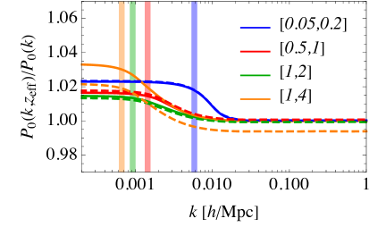
Refer to caption
Refer to caption
Refer to caption
Refer to caption
Refer to caption
Refer to caption
Figure 4: We plot the ratio between the power spectrum within the effective redshift approximation and the full redshift dependence for the monopole (top panels), the dipole (middle panels) and the quadrupole (bottom panels). The different colors are associated to the following constant redshift selection functions: [0.05,0.2]0.050.2[0.05,0.2] blue, [0.5,1]0.51[0.5,1] red, [1,2]12[1,2] green and [1,4]14[1,4] orange. Solid lines refer to the theoretical effective redshift defined in Eq. (2.18), while dashed lines to the volume weighted mean redshift, see Eq. (2.25). The vertical lines correspond to the largest scales probed by the survey, i.e. 2π/(2r(zmax)sinθmax)2𝜋2𝑟subscript𝑧maxsubscript𝜃max2\pi/\left(2r(z_{\rm max})\sin\theta_{\rm max}\right). In the left panels we consider b1=1.5/D1(z)subscript𝑏11.5subscript𝐷1𝑧b_{1}=1.5/D_{1}\left(z\right), while on the right panels b1=1.5subscript𝑏11.5b_{1}=1.5.

The accuracy of the effective approximation is shown in Figure 4, where we plot the ratio between the full prediction, i.e. integrated over s1subscript𝑠1s_{1}, and the power spectrum evaluated at the effective redshift, for the monopole, dipole and quadrupole. The prediction includes only the density plus RSD piece. For the left panels we assumed the linear bias scales with the growth factor, D(z)b1(z)=1.5𝐷𝑧subscript𝑏1𝑧1.5D(z)b_{1}(z)=1.5, while on the right ones we fixed b1(z)=1.5subscript𝑏1𝑧1.5b_{1}(z)=1.5. Different colors show different surveys, and the vertical bars display the largest scales measured in each of them. Continuous lines indicate the prediction evaluated at the zeff,subscript𝑧effz_{\rm eff,\,\ell} (see Eq. (2.18)), which by definition are unbiased at sufficiently high k𝑘k, while dashed ones use the global zeffsubscript𝑧effz_{\rm eff} (see Eq. (2.25)). Notice that for the dipole we only show the global zeffsubscript𝑧effz_{\rm eff} since in the plane parallel limit there is no intrinsic dipole. This figure shows that the effective redshift approximation with the zeff,subscript𝑧effz_{\rm eff,\,\ell}’s is in general a very good approximation, better than a % in all cases except the more unrealistic scenario of a single redshift bin galaxy survey between zmin=1subscript𝑧min1z_{\rm min}=1 and zmax=4subscript𝑧max4z_{\rm max}=4. The global zeffsubscript𝑧effz_{\rm eff} performs slightly worse, and it is less accurate for constant galaxy bias. We also notice that the error introduced by the effective redshift approximation is usually multiplicative, and it can therefore be absorbed in a redefinition of the in principle unknown galaxy bias.

In real data the accuracy of the effective redshift prediction will depend on other observational effects, like completeness, that can be trivially included as additional redshift weights in our theoretical predictions.

5.1.1 Full sky and s/s1𝑠subscript𝑠1s/s_{1} expansion

To obtain the estimated power spectrum we need to convolve the expression of the correlation function with the multipoles of the window function. Because of the finite survey volume, rather than computing the full ξ(s,s1)subscript𝜉𝑠subscript𝑠1\xi_{\ell}(s,s_{1}), a more practical approach for the convolution with the window function is to expand the multipoles in powers of s/s1𝑠subscript𝑠1s/s_{1}

ξ(s1,s)=j(ss1)jξ(j)(s).subscript𝜉subscript𝑠1𝑠subscript𝑗superscript𝑠subscript𝑠1𝑗superscriptsubscript𝜉𝑗𝑠\xi_{\ell}\left(s_{1},s\right)=\sum_{j}\left(\frac{s}{s_{1}}\right)^{j}\xi_{\ell}^{(j)}\left(s\right)\,. (5.7)

Notice that in the above expression the ξ(j)superscriptsubscript𝜉𝑗\xi_{\ell}^{(j)} might still explicit depend on s1subscript𝑠1s_{1} to account for the redshift dependence of the growth factors.

Refer to caption
Refer to caption
Figure 5: We plot the ratio between the monopole of power spectrum expanded up to different order in the wide-angle parameter s/s1𝑠subscript𝑠1s/s_{1} and the full-sky power spectrum. The panels show the four different surveys with increasing redshift coverage from left to right. The vertical orange line indicates k=2π/r(zeff)𝑘2𝜋𝑟subscript𝑧effk=2\pi/r(z_{\rm eff}), while the gray line refers to the largest scales within the survey geometry. In the top panels we consider b1=1.5/D1(z)subscript𝑏11.5subscript𝐷1𝑧b_{1}=1.5/D_{1}\left(z\right), while on the bottom panels b1=1.5subscript𝑏11.5b_{1}=1.5.

The series expansion is certainly a bad approximation close to the survey boundary where the separation s𝑠s could approach the distance to the pair, and it eventually diverges, but the finite size of the window function addresses many of these shortcomings. In Fig. 5 we show the ratio between the monopole of the predicted power spectrum up to a given order in the series expansion, P^L(j)(k)subscriptsuperscript^𝑃𝑗𝐿𝑘\hat{P}^{(j)}_{L}(k), and the full calculation. In all four cases considered we assume a sky fraction fsky=1/3subscript𝑓sky13f_{\rm sky}=1/3 and vary the redshift range of the measurements. We find that the second order expansion in s/s1𝑠subscript𝑠1s/s_{1}, usually employed in the literature [Castorina:2017inr, Beutler:2018vpe], is always a very good approximation up to the survey boundary, indicated by the thick vertical gray line in the panels. The difference of a few % is always well below the expected cosmic variance for these hypothetical surveys. Notice how the presence of the window function makes the flat-sky prediction, the blue lines at 𝒪(s/s1)0𝒪superscript𝑠subscript𝑠10\mathcal{O}(s/s_{1})^{0}, very accurate.

Refer to caption
Refer to caption
Figure 6: We plot the ratio between the quadrupole of the power spectrum expanded up to different orders in the wide-angle parameter s/s1𝑠subscript𝑠1s/s_{1} and the full-sky power spectrum. The four panels show survey geometry with different deepness in redshift. The vertical orange line indicates k=2π/r(zeff)𝑘2𝜋𝑟subscript𝑧effk=2\pi/r(z_{\rm eff}), while the gray line refers to the largest scales within the survey geometry. In the top panels we consider b1=1.5/D1(z)subscript𝑏11.5subscript𝐷1𝑧b_{1}=1.5/D_{1}\left(z\right), while on the bottom panels b1=1.5subscript𝑏11.5b_{1}=1.5.

The same set of plots is shown for the quadrupole in Fig. 6. As expected the series expansion performs slightly worse than for the monopole, but it should be kept in mind that the cosmic variance increases accordingly. The perturbative expansion in s/s1𝑠subscript𝑠1s/s_{1} breaks down at scale larger than k2π/reffsimilar-to𝑘2𝜋subscript𝑟effk\sim 2\pi/r_{\rm eff}, shown as the orange bar in the Figure. Indeed this scale corresponds to s/s11similar-to𝑠subscript𝑠11s/s_{1}\sim 1 in configuration space.

Refer to caption
Refer to caption
Figure 7: We plot the ratio between the dipole of power spectrum expanded up to different orders in the wide-angle parameter s/s1𝑠subscript𝑠1s/s_{1} and the full-sky power spectrum. The four panels show survey geometry with different deepness in redshift. The vertical orange line indicates k=2π/r(zeff)𝑘2𝜋𝑟subscript𝑧effk=2\pi/r(z_{\rm eff}), while the gray line refers to the largest scales within the survey geometry. In the top panels we consider b1=1.5/D1(z)subscript𝑏11.5subscript𝐷1𝑧b_{1}=1.5/D_{1}\left(z\right), while on the bottom panels b1=1.5subscript𝑏11.5b_{1}=1.5.

For the dipole (Fig. 7) the perturbative expansion starts to converge at 𝒪(s/s1)𝒪𝑠subscript𝑠1\mathcal{O}\left(s/s_{1}\right). Because the dipole of the correlation function vanishes for a single tracer, P1(k)subscript𝑃1𝑘P_{1}\left(k\right) in the plane-parallel approximation receives contributions only from the coupling between the window function and other multipoles.

5.2 Lensing Magnification

At fixed pair separation s𝑠s between two observed galaxies, terms like lensing magnification or ISW measure the correlation between points along the lines of sight of the two galaxies. The "non-locality" of such contributions makes harder to understand to which value of k𝑘k in the power spectrum they mostly contribute. In our formalism, however, computing the average of the observed power spectrum requires only the evaluation of the three-dimensional correlation function multipoles. We compute ξ(s1,s2,cosθ)𝜉subscript𝑠1subscript𝑠2𝜃\xi(s_{1},s_{2},\cos\theta) or ξ(s,s1,μ)𝜉𝑠subscript𝑠1𝜇\xi(s,s_{1},\mu) using FFTs, and then Monte-Carlo or quadrature methods for the integrals along the LOS and the projection into multipoles.

In this section we focus on lensing magnification, which enters the power spectrum at the same order in derivatives as the standard density and RSD terms. As mentioned before, we set sb=0subscript𝑠𝑏0s_{b}=0 as its value changes only the normalization of the lensing contribution to the power spectrum.

Fig. 8 shows in red the contribution of lensing magnification to the monopole and quadrupole of the power spectrum, which can be compared to the RSD term (including wide angle effects) in blue. Both curves include the effect of the window function, but not the integral constraint. For reference the flat-sky linear theory prediction in absence of a window function is shown as the dashed black line. Fig. 9 instead shows, again in red, the relative difference between the RSD power spectrum and the RSD plus lensing power spectrum. Because we are adding the different contributions we can now consistently subtract the integral constraint. As expected lensing magnification is a tiny effect for low redshift surveys with a small extension in redshift, as displayed in the leftmost panels. In this case, for both the monopole and the quadrupole we find lensing magnification leads to sub-% changes on the total power spectrum. Moving to higher redshift and wider redshift ranges the effect of lensing increases, reaching tens of percent for the monopole and 𝒪(1)𝒪1\mathcal{O}(1) for the quadrupole in our most unrealistic setup of a single redshift bin between z=1𝑧1z=1 and z=4𝑧4z=4 over one third of the sky. We remark that the spikes in the lower panels of Fig. 9 appear because the RSD quadrupole crosses zero, see Fig. 3. The larger effect on the quadrupole can be understood by noticing that lensing magnification contains a transverse Laplacian, which depends strongly on μ𝜇\mu and it is therefore more sensitive to the non uniform weighting of higher multipoles. The information carried by the lensing magnification effect is thus spread over several multipoles. Note for instance in Fig 8 that the lensing quadrupole, red line in the lower panels, is usually larger than the lensing monopole, red lines in the upper panels. Interestingly this could open the possibility to detect the lensing contribution by measuring the power spectrum at large scales for higher multipoles where the Newtonian effects are strongly suppressed.

Investigations with more realistic angular masks and selection function are certainly needed, but our analysis indicates that lensing magnification will likely not play a major role in cosmological parameter inference in spectroscopic surveys.
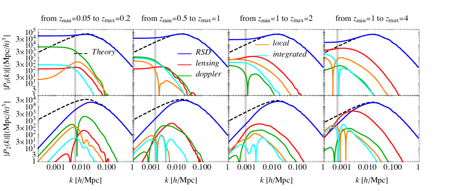
Refer to caption
Figure 8: We plot the contributions of all the relativistic effects to the monopole (top panels) and quadrupole (bottom panels) of the power spectrum. Each relativistic effect includes also the correlation with the other effects listed above it in the legend. We remark that we are not considering the integral constraints in this figure, since we want to highlight the contribution of the single relativistic effects. The vertical lines correspond to the largest scales probed by the survey, i.e. 2π/(2r(zmax)sinθmax)2𝜋2𝑟subscript𝑧maxsubscript𝜃max2\pi/\left(2r(z_{\rm max})\sin\theta_{\rm max}\right).

5.3 The observed galaxy power spectrum

In this section we finally discuss all the relativistic effects and their effect on the observed power spectrum. As we can see from Figs. 8 - 9, the relevance of the different effects changes with the survey volume and redshift coverage. In Fig. 9, as discussed in the previous Section, each line shows the ratio between the RSD prediction and RSD plus all the GR terms above in the Figure legend. For example the green line is the relative difference between the RSD term and RSD plus lensing and Doppler terms, and so on.

At low redshifts the main contribution is due to the Doppler effects. This behaviour is well explained by the presence of the dependence on 1/(r)1𝑟1/(\mathcal{H}r) of such terms. In our low redshift survey, the Doppler terms are approximately 5% and 10% of the RSD ones for the monopole and the quadrupole respectively. They are therefore much larger than the lensing magnification. Indeed, lensing is an integrated effect from the source to the observer and its contribution growths by summing up several lensing deflections along the line of sight. Local and integrated terms are subdominant at such low redshift. Notice that all GR terms are proportional to P(k)kn𝑃𝑘superscript𝑘𝑛P(k)k^{n} for some n<0𝑛0n<0, until the window function dominates.

At intermediate redshifts, between zmin=0.5subscript𝑧min0.5z_{\rm min}=0.5 and zmax=1subscript𝑧max1z_{\rm max}=1, lensing become comparable to the Doppler terms, and the other local and integrated terms also grow. For this survey, GR corrections are still sub-% for the monopole and approximately 10% for the quadrupole on the largest scales. Interestingly, in our setup, the GR effects are minimized for a survey at intermediate redshifts, as the Doppler effect starts to decrease and lensing magnification has not yet taken over.

Moving to the high redshift Universe, in our survey between zmin=1subscript𝑧min1z_{\rm min}=1 and zmax=2subscript𝑧max2z_{\rm max}=2 or zmin=1subscript𝑧min1z_{\rm min}=1 and zmax=4subscript𝑧max4z_{\rm max}=4 the lensing magnification dominates over all other terms, and the conclusions we reached in the previous section apply.

Our results indicate that for current and upcoming LSS surveys, cosmological inference from Baryon Acoustic Oscillations and the shape of the power spectrum on quasi-linear scales is largely unaffected by GR effects, which are sub per mille corrections to the RSD term.
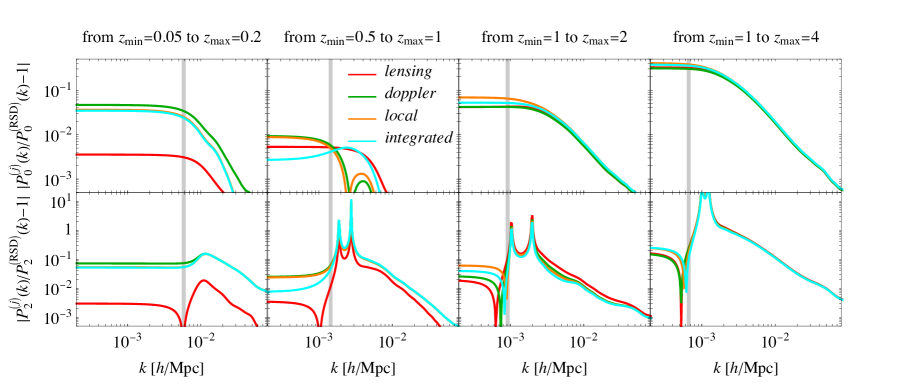
Refer to caption
Figure 9: We show the ratio between the multipoles (monopole on top panels and quadrupole in the bottom ones) sourced by RSD with respect to the other relativistic effects. We add the effect one by one, such that the lensing line contains also RSD, the doppler line also lensing and RSD, and so on. In the Integral Constraint we include the same effects. The vertical lines correspond to the largest scales probed by the survey, i.e. 2π/(2r(zmax)sinθmax)2𝜋2𝑟subscript𝑧maxsubscript𝜃max2\pi/\left(2r(z_{\rm max})\sin\theta_{\rm max}\right).

We conclude this section by investigating the accuracy of the effective redshift approximation once we include all the relativistic effects. Our findings are shown in Fig. 10, assuming the linear bias scales as b1(z)D(z)=1.5subscript𝑏1𝑧𝐷𝑧1.5b_{1}(z)D(z)=1.5. While we know that in principle the redshift evolution of the integrated terms, including lensing, is scale-dependent, because the latter are a relatively small correction on top of the standard RSD power spectrum the effective redshift approximation works extremely well also in the presence of relativistic corrections, with 5% differences in the monopole only for the very extended survey between zmin=1subscript𝑧min1z_{\rm min}=1 and zmax=4subscript𝑧max4z_{\rm max}=4 shown in the rightmost column101010We caution the reader that this approximation may fail if one is interested in the integrated terms only..
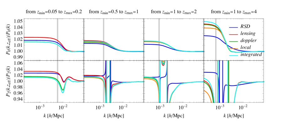
Refer to caption
Figure 10: We show the accuracy of the effective redshift approximation (according to Eq. (2.18)) by including all the relativistic effects. Similarly to Fig. 9 we add each effect one by one. The top panels refer to the monopole, while the bottom ones to the quadrupole. The vertical lines correspond to the largest scales probed by the survey, i.e. 2π/(2r(zmax)sinθmax)2𝜋2𝑟subscript𝑧maxsubscript𝜃max2\pi/\left(2r(z_{\rm max})\sin\theta_{\rm max}\right).

6 Conclusions

In this work we presented the first computation, in General Relativity, for the ensemble average of the Fourier space estimators traditionally used in the galaxy power spectrum analyses of spectroscopic surveys. We clarified the relation between what is measured and what is predicted and how different estimators effectively perform different compressions of the data. Since GR corrections are important on large scales, a meaningful calculation must include observational effects like the presence of an angular mask, of a redshift selection function, and of the Integral Constraint. We implemented the presence of an arbitrary window function in the exact way, highlighting which assumptions could be employed to simplify the computation in certain situations.

A prerequisite for the GR calculation is the understanding of the IR divergences, and more generally of the IR sensitivity, of the three dimensional correlation function of the galaxy overdensity field. We showed for the first time that these effects are not present once all the terms in the expression for the galaxy number counts are taken into account, and the full calculation for any observable is finite and insensitive to the large scale cutoff of the theory. We were able to trace back this cancellation to the presence of the Weinberg adiabatic mode [Weinberg:2003sw] and of the Consistency relations for LSS [Creminelli2013, Peloso2013, Kehagias2013]. From these results, our calculations therefore inherit the underlying conditions of validity such as adiabatic and Gaussian initial conditions, and diffeomorphism invariance. Our expression for the observed power spectrum differs from the one in Ref. [Grimm:2020ays], with whom we therefore disagree on the interpretation of the relevance of the IR contributions to the power spectrum. Since our definition coincides with the power spectrum routinely measured in galaxy surveys we conclude that the power spectrum proposed in Ref. [Grimm:2020ays] does not necessarily correspond to an observable quantity.

We then computed the observed power spectrum in four different hypothetical surveys, covering one third of the sky at different redshifts. We first confirmed earlier work in the literature on wide angle RSD, which we found to be a few % of the total signal on very large scales. We also validated the series expansion approach to wide angle RSD, which is sub-% accurate once the first few terms in the series have been included. We then checked the accuracy of using an effective redshift to model the clustering signal, and found that for our choice of radial selection functions it has a negligible impact, unless in a very extended survey between z=1𝑧1z=1 and z=4𝑧4z=4. The validity of the effective redshift approximation depends on both the redshift evolution of the sample and the selection function, therefore any conclusions on more realistic galaxy samples than what we considered here should rely on the full machinery provided in this work.

We then showed for the first time the impact of lensing magnification on the multipoles of the observed power spectrum, finding it is not a significant effect at low-z𝑧z but it can account for the 5-10% of the monopole and the quadrupole at large scales for sufficiently realistic high redshift surveys.

A summary of our results, including all GR effects, can be found in Fig. 8 - 9. For low-redshift surveys the Doppler term is the most important GR contribution, up to 5-10% of the total power, while at intermediate and high redshift lensing magnification becomes more significant. Other GR effects like ISW, time delays, and local terms are in general negligible. Being the GR effects a small contribution to the observed multipoles, the effective redshift approximation remains valid in most cases considered.

There are several directions along which this work can be extended. One of our main motivation was to understand the importance of GR effects when constraining local PNG with scale dependent bias. We presented the expression for the average of the Fourier Space estimator, but we cannot yet quantitatively address any possible degeneracy of GR terms with PNG because we miss an expression for the covariance of the measured power spectrum including GR effects and the window function. The mask indeed makes the covariance of the power spectrum non diagonal on very large scales, and so far only approximate analytical calculations in the flat sky limit have been proposed [Wadekar:2019rdu]. Such an investigation is subject of work in progress by the authors [futureFNL].

Our implementation of the Yamamoto estimator uses the endpoint LOS, but several other choices are possible. In particular, for analyses aiming at the Doppler terms a symmetric choice of LOS, like the bisector, is preferable because it sets to zero purely geometric dipoles. Also in this case the power spectrum can be measured with FFTs [Castorina2018, Philcox2021], and all our calculations go through unchanged with the replacement of s1subscript𝑠1s_{1} with the length of the new LOS. It is also well known that Yamamoto-like estimators are not statistically optimal on large scales [Tegmark:1997yq]. It is therefore natural to ask how to incorporate GR effects in optimal quadratic estimators of the power spectrum, which are traditionally implemented using a flat-sky RSD model [Philcox2020]. As a final remark we note that the full GR calculation is computationally much slower than the Newtonian one. However given the smallness of many GR terms, one could imagine resorting to the flat-sky approximation in some cases and obtain order of magnitudes speed up of the numerical calculations [Jelic-Cizmek:2020jsn]. We plan to return to these interesting problems in forthcoming publications.

Acknowledgments

ED (No. 171494 and 171506) acknowledges financial support from the Swiss National Science Foundation during the first stages of this project. We would like to thank the participants of the workshop "Relativistic Aspects of Large Scale Structure", where this work was first presented, for discussion. We thank Matteo Foglieni for finding several typos in the equations presented in Appendices of the first version of this work.

Appendix A Azimuthally symmetric window function

In this appendix we provide explicit expressions for the convolution with an azimuthally symmetric window function

ϕ(𝐬1)=ϕ(s1)W(θ1)=ϕ(s1)Θ(θmaxθ1).italic-ϕsubscript𝐬1italic-ϕsubscript𝑠1𝑊subscript𝜃1italic-ϕsubscript𝑠1Θsubscript𝜃maxsubscript𝜃1\phi\left({\bf{s}}_{1}\right)=\phi\left(s_{1}\right)W\left(\theta_{1}\right)=\phi\left(s_{1}\right)\Theta\left(\theta_{\rm max}-\theta_{1}\right)\,. (A.1)

For this survey geometry Eq. (2.16) reduces to

F1(s1,s)=23(123000)2(23+1)ϕ2(s1,s)A3(ss1)subscript𝐹subscript1subscript𝑠1𝑠subscriptsubscript2subscript3superscriptsubscript1subscript2subscript300022subscript31subscriptitalic-ϕsubscript2subscript𝑠1𝑠subscript𝐴subscript3𝑠subscript𝑠1F_{\ell_{1}}\left(s_{1},s\right)=\sum_{\ell_{2}\ell_{3}}\left(\begin{array}[]{ccc}\ell_{1}&\ell_{2}&\ell_{3}\\ 0&0&0\end{array}\right)^{2}\left(2\ell_{3}+1\right)\phi_{\ell_{2}}\left(s_{1},s\right)A_{\ell_{3}}\left(\frac{s}{s_{1}}\right) (A.2)

where

A(x)=2π0θmaxdθ1sinθ10πdθsinθ02πdϕΘ(cosθ2cosθmax)(𝐬^1𝐬^)subscript𝐴𝑥2𝜋superscriptsubscript0subscript𝜃maxdifferential-dsubscript𝜃1subscript𝜃1superscriptsubscript0𝜋differential-d𝜃𝜃superscriptsubscript02𝜋differential-ditalic-ϕΘsubscript𝜃2subscript𝜃maxsubscriptsubscript^𝐬1^𝐬A_{\ell}\left(x\right)=2\pi\int_{0}^{\theta_{\rm max}}{\rm d}\theta_{1}\sin\theta_{1}\int_{0}^{\pi}{\rm d}\theta\sin\theta\int_{0}^{2\pi}{\rm d}\phi\Theta\left(\cos\theta_{2}-\cos\theta_{\rm max}\right)\mathcal{L}_{\ell}\left(\hat{\bf{s}}_{1}\cdot\hat{\bf{s}}\right) (A.3)

and

ϕ(s1,s)=2+1211dμϕ(s2)(μ).subscriptitalic-ϕsubscript𝑠1𝑠212superscriptsubscript11differential-d𝜇italic-ϕsubscript𝑠2subscript𝜇\phi_{\ell}\left(s_{1},s\right)=\frac{2\ell+1}{2}\int_{-1}^{1}{\rm d}\mu\phi\left(s_{2}\right)\mathcal{L}_{\ell}\left(\mu\right)\,. (A.4)

For a top-hat redshift selection function we also have that

ϕ(s1)=Θ(s1smin)Θ(smaxs1),italic-ϕsubscript𝑠1Θsubscript𝑠1subscript𝑠minΘsubscript𝑠maxsubscript𝑠1\phi\left(s_{1}\right)=\Theta\left(s_{1}-s_{\rm min}\right)\Theta\left(s_{\rm max}-s_{1}\right)\,, (A.5)

and we can perform the integral analytically obtaining

ϕ(s2)=ϕ(s12+s2+2s1sμ)=ϕ(s1,s)(μ)italic-ϕsubscript𝑠2italic-ϕsuperscriptsubscript𝑠12superscript𝑠22subscript𝑠1𝑠𝜇subscriptsubscriptitalic-ϕsubscript𝑠1𝑠subscript𝜇\displaystyle\phi\left(s_{2}\right)=\phi\left(\sqrt{s_{1}^{2}+s^{2}+2s_{1}s\mu}\right)=\sum_{\ell}\phi_{\ell}\left(s_{1},s\right)\mathcal{L}_{\ell}\left(\mu\right) (A.6)

where

ϕ(s1,s)subscriptitalic-ϕsubscript𝑠1𝑠\displaystyle\phi_{\ell}\left(s_{1},s\right) =\displaystyle= 2+12Θ(smax(ss1))212Θsubscript𝑠max𝑠subscript𝑠1\displaystyle\frac{2\ell+1}{2}\Theta\left(s_{\rm max}-\left(s-s_{1}\right)\right)
[Θ(smaxs2(s1,s,1))Θ(s2(s1,s,1)smin)11dμ(μ)\displaystyle\left[\Theta\left(s_{\rm max}-s_{2}\left(s_{1},s,1\right)\right)\Theta\left(s_{2}\left(s_{1},s,-1\right)-s_{\rm min}\right)\int_{-1}^{1}{\rm d}\mu\ \mathcal{L}_{\ell}\left(\mu\right)\right.
+Θ(smax+s2(s1,s,1))Θ(s2(s1,s,1)smin)1(smax2s2s12)/(2ss1)dμ(μ)Θsubscript𝑠maxsubscript𝑠2subscript𝑠1𝑠1Θsubscript𝑠2subscript𝑠1𝑠1subscript𝑠minsuperscriptsubscript1superscriptsubscript𝑠max2superscript𝑠2superscriptsubscript𝑠122𝑠subscript𝑠1differential-d𝜇subscript𝜇\displaystyle\left.+\Theta\left(-s_{\rm max}+s_{2}\left(s_{1},s,1\right)\right)\Theta\left(s_{2}\left(s_{1},s,-1\right)-s_{\rm min}\right)\int_{-1}^{\left(s_{\rm max}^{2}-s^{2}-s_{1}^{2}\right)/\left(2ss_{1}\right)}\!\!\!\!\!\!\!\!\!\!\!\!\!\!\!\!\!\!{\rm d}\mu\ \mathcal{L}_{\ell}\left(\mu\right)\right.
+Θ(smaxs2(s1,s,1))Θ(s2(s1,s,1)+smin)(smin2s2s12)/(2ss1)1dμ(μ)Θsubscript𝑠maxsubscript𝑠2subscript𝑠1𝑠1Θsubscript𝑠2subscript𝑠1𝑠1subscript𝑠minsuperscriptsubscriptsuperscriptsubscript𝑠min2superscript𝑠2superscriptsubscript𝑠122𝑠subscript𝑠11differential-d𝜇subscript𝜇\displaystyle\left.+\Theta\left(s_{\rm max}-s_{2}\left(s_{1},s,1\right)\right)\Theta\left(-s_{2}\left(s_{1},s,-1\right)+s_{\rm min}\right)\int_{\left(s_{\rm min}^{2}-s^{2}-s_{1}^{2}\right)/\left(2ss_{1}\right)}^{1}\!\!\!\!\!\!\!\!\!\!\!\!\!\!\!\!\!\!{\rm d}\mu\ \mathcal{L}_{\ell}\left(\mu\right)\right.
+Θ(smax+s2(s1,s,1))Θ(s2(s1,s,1)+smin)(smin2s2s12)/(2ss1)(smax2s2s12)/(2ss1)dμ(μ)]\displaystyle\left.+\Theta\left(-s_{\rm max}+s_{2}\left(s_{1},s,1\right)\right)\Theta\left(-s_{2}\left(s_{1},s,-1\right)+s_{\rm min}\right)\int_{\left(s_{\rm min}^{2}-s^{2}-s_{1}^{2}\right)/\left(2ss_{1}\right)}^{\left(s_{\rm max}^{2}-s^{2}-s_{1}^{2}\right)/\left(2ss_{1}\right)}\!\!\!\!\!\!\!\!\!\!\!\!\!\!\!\!\!\!{\rm d}\mu\ \mathcal{L}_{\ell}\left(\mu\right)\right]

For this symmetric window function we can also pursuit a different path, without relying on the calculation of the multipoles of the correlation function. In the case of relativistic effects integrated from the source to the observer, such approach can lead to a simpler numerical evaluation. In this case we start considering the expectation value of the power spectrum estimator

P^L(k)delimited-⟨⟩subscript^𝑃𝐿𝑘\displaystyle\langle\hat{P}_{L}\left(k\right)\rangle =\displaystyle= 2L+1AdΩk4πd3s1d3s2ξ(s1,s,𝐬^1𝐬^)ϕ(𝐬1)ϕ(𝐬2)ei𝐤𝐬L(𝐤^𝐬^1)2𝐿1𝐴𝑑subscriptΩ𝑘4𝜋superscriptd3subscript𝑠1superscriptd3subscript𝑠2𝜉subscript𝑠1𝑠subscript^𝐬1^𝐬italic-ϕsubscript𝐬1italic-ϕsubscript𝐬2superscript𝑒𝑖𝐤𝐬subscript𝐿^𝐤subscript^𝐬1\displaystyle\frac{2L+1}{A}\int\frac{d\Omega_{k}}{4\pi}\int{\rm d}^{3}s_{1}{\rm d}^{3}s_{2}\xi\left(s_{1},s,\hat{\bf{s}}_{1}\cdot\hat{\bf{s}}\right)\phi\left({\bf{s}}_{1}\right)\phi\left({\bf{s}}_{2}\right)e^{-i{\bf{k}}\cdot{\bf{s}}}\mathcal{L}_{L}\left(\hat{\bf{k}}\cdot\hat{\bf{s}}_{1}\right) (A.8)
=\displaystyle= 2L+1A(i)Ld3s1d3sξ(s1,s,𝐬^1𝐬^)ϕ(𝐬1)ϕ(𝐬2)jL(ks)L(𝐬^𝐬^1)2𝐿1𝐴superscript𝑖𝐿superscriptd3subscript𝑠1superscriptd3𝑠𝜉subscript𝑠1𝑠subscript^𝐬1^𝐬italic-ϕsubscript𝐬1italic-ϕsubscript𝐬2subscript𝑗𝐿𝑘𝑠subscript𝐿^𝐬subscript^𝐬1\displaystyle\frac{2L+1}{A}\left(-i\right)^{L}\int{\rm d}^{3}s_{1}{\rm d}^{3}s\xi\left(s_{1},s,\hat{\bf{s}}_{1}\cdot\hat{\bf{s}}\right)\phi\left({\bf{s}}_{1}\right)\phi\left({\bf{s}}_{2}\right)j_{L}\left(ks\right)\mathcal{L}_{L}\left(\hat{\bf{s}}\cdot\hat{\bf{s}}_{1}\right)

where in the second line we have changed the integration variables (d3s1d3s2d3s1d3ssuperscriptd3subscript𝑠1superscriptd3subscript𝑠2superscriptd3subscript𝑠1superscriptd3𝑠{\rm d}^{3}s_{1}{\rm d}^{3}s_{2}\rightarrow{\rm d}^{3}s_{1}{\rm d}^{3}s). By explicitly using the symmetry of the survey geometry we obtain

P^L(k)delimited-⟨⟩subscript^𝑃𝐿𝑘\displaystyle\langle\hat{P}_{L}\left(k\right)\rangle =\displaystyle= 2L+1A(i)L2πds1s12dss2dθsinθdθ1sinθ1dφξ(s1,s,𝐬^1𝐬^)2𝐿1𝐴superscript𝑖𝐿2𝜋differential-dsubscript𝑠1superscriptsubscript𝑠12differential-d𝑠superscript𝑠2differential-d𝜃𝜃dsubscript𝜃1subscript𝜃1d𝜑𝜉subscript𝑠1𝑠subscript^𝐬1^𝐬\displaystyle\frac{2L+1}{A}\left(-i\right)^{L}2\pi\int{\rm d}s_{1}s_{1}^{2}{\rm d}ss^{2}{\rm d}\theta\sin\theta{\rm d}\theta_{1}\sin\theta_{1}{\rm d}\varphi\xi\left(s_{1},s,\hat{\bf{s}}_{1}\cdot\hat{\bf{s}}\right) (A.9)
ϕ(s1)ϕ(s2)jL(ks)W(θ1)W(θ2)L(𝐬^𝐬^1)italic-ϕsubscript𝑠1italic-ϕsubscript𝑠2subscript𝑗𝐿𝑘𝑠𝑊subscript𝜃1𝑊subscript𝜃2subscript𝐿^𝐬subscript^𝐬1\displaystyle\phi\left(s_{1}\right)\phi\left(s_{2}\right)j_{L}\left(ks\right)W\left(\theta_{1}\right)W\left(\theta_{2}\right)\mathcal{L}_{L}\left(\hat{\bf{s}}\cdot\hat{\bf{s}}_{1}\right)
=\displaystyle= 2L+1A(i)L4πds1s12dss2dθsinθdθ1sinθ1dy1y2ξ(s1,s,𝐬^1𝐬^)2𝐿1𝐴superscript𝑖𝐿4𝜋differential-dsubscript𝑠1superscriptsubscript𝑠12differential-d𝑠superscript𝑠2differential-d𝜃𝜃dsubscript𝜃1subscript𝜃1𝑑𝑦1superscript𝑦2𝜉subscript𝑠1𝑠subscript^𝐬1^𝐬\displaystyle\frac{2L+1}{A}\left(-i\right)^{L}4\pi\int{\rm d}s_{1}s_{1}^{2}{\rm d}ss^{2}{\rm d}\theta\sin\theta{\rm d}\theta_{1}\sin\theta_{1}\frac{dy}{\sqrt{1-y^{2}}}\xi\left(s_{1},s,\hat{\bf{s}}_{1}\cdot\hat{\bf{s}}\right)
ϕ(s1)ϕ(s2)jL(ks)W(θ1)W(θ2)L(𝐬^𝐬^1)italic-ϕsubscript𝑠1italic-ϕsubscript𝑠2subscript𝑗𝐿𝑘𝑠𝑊subscript𝜃1𝑊subscript𝜃2subscript𝐿^𝐬subscript^𝐬1\displaystyle\phi\left(s_{1}\right)\phi\left(s_{2}\right)j_{L}\left(ks\right)W\left(\theta_{1}\right)W\left(\theta_{2}\right)\mathcal{L}_{L}\left(\hat{\bf{s}}\cdot\hat{\bf{s}}_{1}\right)
=\displaystyle= 2L+1A(i)L4πds1s12dss2dμξ(s1,s,μ)ϕ(s1)jL(ks)ϕ(s2)L(μ)2𝐿1𝐴superscript𝑖𝐿4𝜋differential-dsubscript𝑠1superscriptsubscript𝑠12differential-d𝑠superscript𝑠2differential-d𝜇𝜉subscript𝑠1𝑠𝜇italic-ϕsubscript𝑠1subscript𝑗𝐿𝑘𝑠italic-ϕsubscript𝑠2subscript𝐿𝜇\displaystyle\frac{2L+1}{A}\left(-i\right)^{L}4\pi\int{\rm d}s_{1}s_{1}^{2}{\rm d}ss^{2}{\rm d}\mu\xi\left(s_{1},s,\mu\right)\phi\left(s_{1}\right)j_{L}\left(ks\right)\phi\left(s_{2}\right)\mathcal{L}_{L}\left(\mu\right)
dθ1dθW(θ1)W(θ2)Θ(μcos(θ+θ1))Θ(cos(θθ1)μ)differential-dsubscript𝜃1differential-d𝜃𝑊subscript𝜃1𝑊subscript𝜃2Θ𝜇𝜃subscript𝜃1Θ𝜃subscript𝜃1𝜇\displaystyle\int{\rm d}\theta_{1}{\rm d}\theta W\left(\theta_{1}\right)W\left(\theta_{2}\right)\Theta\left(\mu-\cos\left(\theta+\theta_{1}\right)\right)\Theta\left(\cos\left(\theta-\theta_{1}\right)-\mu\right)
sinθ1sinθ(sinθsinθ1)2(cosθcosθ1μ)2subscript𝜃1𝜃superscript𝜃subscript𝜃12superscript𝜃subscript𝜃1𝜇2\displaystyle\frac{\sin\theta_{1}\sin\theta}{\sqrt{\left(\sin\theta\sin\theta_{1}\right)^{2}-\left(\cos\theta\cos\theta_{1}-\mu\right)^{2}}}
=\displaystyle= 2L+1A(i)Lds1s12dss2dμξ(s1,s,μ)2𝐿1𝐴superscript𝑖𝐿differential-dsubscript𝑠1superscriptsubscript𝑠12differential-d𝑠superscript𝑠2differential-d𝜇𝜉subscript𝑠1𝑠𝜇\displaystyle\frac{2L+1}{A}\left(-i\right)^{L}\int{\rm d}s_{1}s_{1}^{2}{\rm d}ss^{2}{\rm d}\mu\xi\left(s_{1},s,\mu\right)
ϕ(s1)jL(ks)ϕ(s2)L(μ)F(ss1,μ)italic-ϕsubscript𝑠1subscript𝑗𝐿𝑘𝑠italic-ϕsubscript𝑠2subscript𝐿𝜇𝐹𝑠subscript𝑠1𝜇\displaystyle\phi\left(s_{1}\right)j_{L}\left(ks\right)\phi\left(s_{2}\right)\mathcal{L}_{L}\left(\mu\right)F\left(\frac{s}{s_{1}},\mu\right)

where we have introduced

F(x,μ)𝐹𝑥𝜇\displaystyle F\left(x,\mu\right) =\displaystyle= 4π0θmaxdθ10πdθΘ(xcosθ+cosθ1x2+1+2xμcosθmax)Θ(μcos(θ+θ1))4𝜋superscriptsubscript0subscript𝜃maxdifferential-dsubscript𝜃1superscriptsubscript0𝜋differential-d𝜃Θ𝑥𝜃subscript𝜃1superscript𝑥212𝑥𝜇subscript𝜃maxΘ𝜇𝜃subscript𝜃1\displaystyle 4\pi\int_{0}^{\theta_{\rm max}}{\rm d}\theta_{1}\int_{0}^{\pi}{\rm d}\theta\ \Theta\left(\frac{x\cos\theta+\cos\theta_{1}}{\sqrt{x^{2}+1+2x\mu}}-\cos\theta_{\rm max}\right)\Theta\left(\mu-\cos\left(\theta+\theta_{1}\right)\right) (A.10)
Θ(cos(θθ1)μ)sinθ1sinθ(sinθsinθ1)2(cosθcosθ1μ)2.Θ𝜃subscript𝜃1𝜇subscript𝜃1𝜃superscript𝜃subscript𝜃12superscript𝜃subscript𝜃1𝜇2\displaystyle\Theta\left(\cos\left(\theta-\theta_{1}\right)-\mu\right)\frac{\sin\theta_{1}\sin\theta}{\sqrt{\left(\sin\theta\sin\theta_{1}\right)^{2}-\left(\cos\theta\cos\theta_{1}-\mu\right)^{2}}}\,.

We can see that this simplified approach fully agree with Eqs. (2.1-2.16). We can easily relate Eq. (A.9) with Eq. (2.1) through

ϕ(s2)L(μ)F(ss1,μ)=,1(L1000)2(21+1)2+12(μ)F1(s1,s).italic-ϕsubscript𝑠2subscript𝐿𝜇𝐹𝑠subscript𝑠1𝜇subscriptsubscript1superscript𝐿subscript100022subscript11212subscript𝜇subscript𝐹subscript1subscript𝑠1𝑠\displaystyle\phi\left(s_{2}\right)\mathcal{L}_{L}\left(\mu\right)F\left(\frac{s}{s_{1}},\mu\right)=\sum_{\ell,\ell_{1}}\left(\begin{array}[]{ccc}L&\ell&\ell_{1}\\ 0&0&0\end{array}\right)^{2}\left(2\ell_{1}+1\right)\frac{2\ell+1}{2}\mathcal{L}_{\ell}\left(\mu\right)F_{\ell_{1}}\left(s_{1},s\right)\,. (A.13)

In particular, for the monopole (L=0𝐿0L=0) we have

F(ss1,μ)ϕ(s2)=2+12(μ)F(s1,s).𝐹𝑠subscript𝑠1𝜇italic-ϕsubscript𝑠2subscript212subscript𝜇subscript𝐹subscript𝑠1𝑠F\left(\frac{s}{s_{1}},\mu\right)\phi\left(s_{2}\right)=\sum_{\ell}\frac{2\ell+1}{2}\mathcal{L}_{\ell}\left(\mu\right)F_{\ell}\left(s_{1},s\right)\,. (A.14)

Appendix B Relativistic correlation function

The full relativistic correlation function can be written as

ξ𝒪𝒪(s1,s2,cosθ=𝐬^1𝐬^2)superscript𝜉𝒪superscript𝒪subscript𝑠1subscript𝑠2𝜃subscript^𝐬1subscript^𝐬2\displaystyle\xi^{\mathcal{O}\mathcal{O}^{\prime}}\left(s_{1},s_{2},\cos\theta=\hat{\bf{s}}_{1}\cdot\hat{\bf{s}}_{2}\right) (B.1)
=\displaystyle= i,nJni𝒪𝒪(s1,s2,cosθ)D1(s1)D1(s2)Iin(s)subscript𝑖𝑛superscriptsubscript𝐽𝑛𝑖𝒪superscript𝒪subscript𝑠1subscript𝑠2𝜃subscript𝐷1subscript𝑠1subscript𝐷1subscript𝑠2subscriptsuperscript𝐼𝑛𝑖𝑠\displaystyle\sum_{i,n}J_{ni}^{\mathcal{O}\mathcal{O}^{\prime}}\left(s_{1},s_{2},\cos\theta\right)D_{1}\left(s_{1}\right)D_{1}\left(s_{2}\right)I^{n}_{i}\left(s\right)
+i,nJni𝒪𝒪(s1,s2,cosθ)D1(s1)Iin(s1)+i,nJni𝒪𝒪(s2,s1,cosθ)D1(s2)Iin(s2)subscript𝑖𝑛superscriptsubscript𝐽𝑛𝑖𝒪superscript𝒪subscript𝑠1subscript𝑠2𝜃subscript𝐷1subscript𝑠1subscriptsuperscript𝐼𝑛𝑖subscript𝑠1subscript𝑖𝑛superscriptsubscript𝐽𝑛𝑖𝒪superscript𝒪subscript𝑠2subscript𝑠1𝜃subscript𝐷1subscript𝑠2subscriptsuperscript𝐼𝑛𝑖subscript𝑠2\displaystyle+\sum_{i,n}J_{ni}^{\mathcal{O}\mathcal{O}^{\prime}}\left(s_{1},s_{2},{\cos\theta}\right)D_{1}\left(s_{1}\right)I^{n}_{i}\left(s_{1}\right)+\sum_{i,n}J_{ni}^{\mathcal{O}\mathcal{O}^{\prime}}\left(s_{2},s_{1},{\cos\theta}\right)D_{1}\left(s_{2}\right)I^{n}_{i}\left(s_{2}\right)
+D1(s2)0s1dχ1i,nJni𝒪𝒪(s1,s2,cosθ,χ1)Iin(Δχ1)subscript𝐷1subscript𝑠2superscriptsubscript0subscript𝑠1differential-dsubscript𝜒1subscript𝑖𝑛superscriptsubscript𝐽𝑛𝑖𝒪superscript𝒪subscript𝑠1subscript𝑠2𝜃subscript𝜒1subscriptsuperscript𝐼𝑛𝑖Δsubscript𝜒1\displaystyle+D_{1}\left(s_{2}\right)\int_{0}^{s_{1}}{\rm d}\chi_{1}\sum_{i,n}J_{ni}^{\mathcal{O}\mathcal{O}^{\prime}}\left(s_{1},s_{2},\cos\theta,\chi_{1}\right)I^{n}_{i}\left(\Delta\chi_{1}\right)
+D1(s1)0s2dχ2i,nJni𝒪𝒪(s1,s2,cosθ,χ2)Iin(Δχ2)subscript𝐷1subscript𝑠1superscriptsubscript0subscript𝑠2differential-dsubscript𝜒2subscript𝑖𝑛superscriptsubscript𝐽𝑛𝑖𝒪superscript𝒪subscript𝑠1subscript𝑠2𝜃subscript𝜒2subscriptsuperscript𝐼𝑛𝑖Δsubscript𝜒2\displaystyle+D_{1}\left(s_{1}\right)\int_{0}^{s_{2}}{\rm d}\chi_{2}\sum_{i,n}J_{ni}^{\mathcal{O}\mathcal{O}^{\prime}}\left(s_{1},s_{2},\cos\theta,\chi_{2}\right)I^{n}_{i}\left(\Delta\chi_{2}\right)
+0s1dχ1i,nJni𝒪𝒪(s1,cosθ,χ1)Iin(χ1)+0s2dχ2i,nJni𝒪𝒪(s2,cosθ,χ2)Iin(χ2)superscriptsubscript0subscript𝑠1differential-dsubscript𝜒1subscript𝑖𝑛superscriptsubscript𝐽𝑛𝑖𝒪superscript𝒪subscript𝑠1𝜃subscript𝜒1subscriptsuperscript𝐼𝑛𝑖subscript𝜒1superscriptsubscript0subscript𝑠2differential-dsubscript𝜒2subscript𝑖𝑛superscriptsubscript𝐽𝑛𝑖𝒪superscript𝒪subscript𝑠2𝜃subscript𝜒2subscriptsuperscript𝐼𝑛𝑖subscript𝜒2\displaystyle+\int_{0}^{s_{1}}{\rm d}\chi_{1}\sum_{i,n}J_{ni}^{\mathcal{O}\mathcal{O}^{\prime}}\left(s_{1},\cos\theta,\chi_{1}\right)I^{n}_{i}\left(\chi_{1}\right)+\int_{0}^{s_{2}}{\rm d}\chi_{2}\sum_{i,n}J_{ni}^{\mathcal{O}\mathcal{O}^{\prime}}\left(s_{2},\cos\theta,\chi_{2}\right)I^{n}_{i}\left(\chi_{2}\right)
+0s1dχ10s2dχ2i,nJni𝒪𝒪(s1,s2,cosθ,χ1,χ2)Iin(χ)superscriptsubscript0subscript𝑠1differential-dsubscript𝜒1superscriptsubscript0subscript𝑠2differential-dsubscript𝜒2subscript𝑖𝑛superscriptsubscript𝐽𝑛𝑖𝒪superscript𝒪subscript𝑠1subscript𝑠2𝜃subscript𝜒1subscript𝜒2subscriptsuperscript𝐼𝑛𝑖𝜒\displaystyle+\int_{0}^{s_{1}}{\rm d}\chi_{1}\int_{0}^{s_{2}}{\rm d}\chi_{2}\sum_{i,n}J_{ni}^{\mathcal{O}\mathcal{O}^{\prime}}\left(s_{1},s_{2},\cos\theta,\chi_{1},\chi_{2}\right)I^{n}_{i}\left(\chi\right)
+Jσ2𝒪𝒪(s1,s2,cosθ)σ2+Jσ4𝒪𝒪(s1,s2,cosθ)σ4,superscriptsubscript𝐽𝜎2𝒪superscript𝒪subscript𝑠1subscript𝑠2𝜃subscript𝜎2superscriptsubscript𝐽𝜎4𝒪superscript𝒪subscript𝑠1subscript𝑠2𝜃subscript𝜎4\displaystyle+J_{\sigma 2}^{\mathcal{O}\mathcal{O}^{\prime}}\left(s_{1},s_{2},\cos\theta\right)\sigma_{2}+J_{\sigma 4}^{\mathcal{O}\mathcal{O}^{\prime}}\left(s_{1},s_{2},\cos\theta\right)\sigma_{4}\,,

where

Δχ2Δsubscript𝜒2\displaystyle\Delta\chi_{2} =\displaystyle= s12+χ222s1χ2cosθsuperscriptsubscript𝑠12superscriptsubscript𝜒222subscript𝑠1subscript𝜒2𝜃\displaystyle\sqrt{s_{1}^{2}+\chi_{2}^{2}-2s_{1}\chi_{2}\cos\theta} (B.2)
Δχ1Δsubscript𝜒1\displaystyle\Delta\chi_{1} =\displaystyle= χ12+s222χ1s2cosθsuperscriptsubscript𝜒12superscriptsubscript𝑠222subscript𝜒1subscript𝑠2𝜃\displaystyle\sqrt{\chi_{1}^{2}+s_{2}^{2}-2\chi_{1}s_{2}\cos\theta} (B.3)
χ𝜒\displaystyle\chi =\displaystyle= χ12+χ222χ1χ2cosθsuperscriptsubscript𝜒12superscriptsubscript𝜒222subscript𝜒1subscript𝜒2𝜃\displaystyle\sqrt{\chi_{1}^{2}+\chi_{2}^{2}-2\chi_{1}\chi_{2}\cos\theta} (B.4)

and we have introduced

σi=dq2π2q2iP(q).subscript𝜎𝑖d𝑞2superscript𝜋2superscript𝑞2𝑖𝑃𝑞\sigma_{i}=\int\frac{{\rm d}q}{2\pi^{2}}q^{2-i}P\left(q\right)\,. (B.5)

The functions Jnisubscript𝐽𝑛𝑖J_{ni} are defined in this Appendix. In this section we summarize the relativistic contribution to the full-sky correlation function. The standard Newtonian contribution has been already derived in Section 5.1. To be consistent with previous derivations [Tansella:2018sld], we present them in terms of the system of coordinates (s1,s2,cosθ=𝐬^1𝐬^2)subscript𝑠1subscript𝑠2𝜃subscript^𝐬1subscript^𝐬2\left(s_{1},s_{2},\cos\theta=\hat{\bf{s}}_{1}\cdot\hat{\bf{s}}_{2}\right) 111111With respect to Ref. [Tansella:2018sld] we include also the terms evaluated at the observer positions. Beyond these additional terms, the reader may need to apply spherical Bessel recursion relations to compare our results with Ref. [Tansella:2018sld]..

B.1 Auto-correlation

B.1.1 Lensing

ξκκ(s1,s2,cosθ)=0r1𝑑χ10r2dχ2[J00κκI00(Δχ)+J02κκI20(Δχ)+J31κκI13(Δχ)+J22κκI22(Δχ)]superscript𝜉𝜅𝜅subscript𝑠1subscript𝑠2𝜃superscriptsubscript0subscript𝑟1differential-dsubscript𝜒1superscriptsubscript0subscript𝑟2differential-dsubscript𝜒2delimited-[]subscriptsuperscript𝐽𝜅𝜅00subscriptsuperscript𝐼00Δ𝜒subscriptsuperscript𝐽𝜅𝜅02subscriptsuperscript𝐼02Δ𝜒subscriptsuperscript𝐽𝜅𝜅31subscriptsuperscript𝐼31Δ𝜒subscriptsuperscript𝐽𝜅𝜅22subscriptsuperscript𝐼22Δ𝜒\xi^{\kappa\kappa}\left(s_{1},s_{2},\cos\theta\right)=\!\!\int_{0}^{r_{1}}\!\!d\chi_{1}\!\int_{0}^{r_{2}}\!\!{\rm d}\chi_{2}\left[J^{\kappa\kappa}_{00}I^{0}_{0}\left(\Delta\chi\right)+J^{\kappa\kappa}_{02}I^{0}_{2}\left(\Delta\chi\right)+J^{\kappa\kappa}_{31}I^{3}_{1}\left(\Delta\chi\right)+J^{\kappa\kappa}_{22}I^{2}_{2}\left(\Delta\chi\right)\right] (B.6)

where Δχ=χ12+χ222χ1χ2cosθΔ𝜒superscriptsubscript𝜒12superscriptsubscript𝜒222subscript𝜒1subscript𝜒2𝜃\Delta\chi=\sqrt{\chi_{1}^{2}+\chi_{2}^{2}-2\chi_{1}\chi_{2}\cos\theta} and (with y=cosθ𝑦𝜃y=\cos\theta)

J00κκsubscriptsuperscript𝐽𝜅𝜅00\displaystyle J^{\kappa\kappa}_{00} =\displaystyle= 3χ12χ224s1s2Δχ4a(χ1)a(χ2)(y21)04ΩM02D1(χ1)(χ1s1)D1(χ2)(χ2s2)3superscriptsubscript𝜒12superscriptsubscript𝜒224subscript𝑠1subscript𝑠2Δsuperscript𝜒4𝑎subscript𝜒1𝑎subscript𝜒2superscript𝑦21superscriptsubscript04superscriptsubscriptΩ𝑀02subscript𝐷1subscript𝜒1subscript𝜒1subscript𝑠1subscript𝐷1subscript𝜒2subscript𝜒2subscript𝑠2\displaystyle-\frac{3\chi_{1}^{2}\chi_{2}^{2}}{4s_{1}s_{2}\Delta\chi^{4}a(\chi_{1})a(\chi_{2})}\left(y^{2}-1\right)\mathcal{H}_{0}^{4}\Omega_{M0}^{2}D_{1}(\chi_{1})(\chi_{1}-s_{1})D_{1}(\chi_{2})(\chi_{2}-s_{2}) (B.7)
(5sb(s1)2)(5sb(s2)2)(8y(χ12+χ22)9χ1χ2y27χ1χ2),5subscript𝑠𝑏subscript𝑠125subscript𝑠𝑏subscript𝑠228𝑦superscriptsubscript𝜒12superscriptsubscript𝜒229subscript𝜒1subscript𝜒2superscript𝑦27subscript𝜒1subscript𝜒2\displaystyle(5s_{b}(s_{1})-2)(5s_{b}(s_{2})-2)\left(8y\left(\chi_{1}^{2}+\chi_{2}^{2}\right)-9\chi_{1}\chi_{2}y^{2}-7\chi_{1}\chi_{2}\right)\,,
J02κκsubscriptsuperscript𝐽𝜅𝜅02\displaystyle J^{\kappa\kappa}_{02} =\displaystyle= 3χ12χ222s1s2Δχ4a(χ1)a(χ2)(y21)04ΩM02D1(χ1)(χ1s1)D1(χ2)(χ2s2)3superscriptsubscript𝜒12superscriptsubscript𝜒222subscript𝑠1subscript𝑠2Δsuperscript𝜒4𝑎subscript𝜒1𝑎subscript𝜒2superscript𝑦21superscriptsubscript04superscriptsubscriptΩ𝑀02subscript𝐷1subscript𝜒1subscript𝜒1subscript𝑠1subscript𝐷1subscript𝜒2subscript𝜒2subscript𝑠2\displaystyle-\frac{3\chi_{1}^{2}\chi_{2}^{2}}{2s_{1}s_{2}\Delta\chi^{4}a(\chi_{1})a(\chi_{2})}\left(y^{2}-1\right)\mathcal{H}_{0}^{4}\Omega_{M0}^{2}D_{1}(\chi_{1})(\chi_{1}-s_{1})D_{1}(\chi_{2})(\chi_{2}-s_{2}) (B.8)
(5sb(s1)2)(5sb(s2)2)(4y(χ12+χ22)3χ1χ2y25χ1χ2),5subscript𝑠𝑏subscript𝑠125subscript𝑠𝑏subscript𝑠224𝑦superscriptsubscript𝜒12superscriptsubscript𝜒223subscript𝜒1subscript𝜒2superscript𝑦25subscript𝜒1subscript𝜒2\displaystyle(5s_{b}(s_{1})-2)(5s_{b}(s_{2})-2)\left(4y\left(\chi_{1}^{2}+\chi_{2}^{2}\right)-3\chi_{1}\chi_{2}y^{2}-5\chi_{1}\chi_{2}\right)\,,
J31κκsubscriptsuperscript𝐽𝜅𝜅31\displaystyle J^{\kappa\kappa}_{31} =\displaystyle= 9yΔχ204ΩM02D1(χ1)(χ1s1)D1(χ2)(χ2s2)(5sb(s1)2)(5sb(s2)2)s1s2a(χ1)a(χ2),9𝑦Δsuperscript𝜒2superscriptsubscript04superscriptsubscriptΩ𝑀02subscript𝐷1subscript𝜒1subscript𝜒1subscript𝑠1subscript𝐷1subscript𝜒2subscript𝜒2subscript𝑠25subscript𝑠𝑏subscript𝑠125subscript𝑠𝑏subscript𝑠22subscript𝑠1subscript𝑠2𝑎subscript𝜒1𝑎subscript𝜒2\displaystyle\frac{9y\Delta\chi^{2}\mathcal{H}_{0}^{4}\Omega_{M0}^{2}D_{1}(\chi_{1})(\chi_{1}-s_{1})D_{1}(\chi_{2})(\chi_{2}-s_{2})(5s_{b}(s_{1})-2)(5s_{b}(s_{2})-2)}{s_{1}s_{2}a(\chi_{1})a(\chi_{2})}\,,\ \ (B.9)
J22κκsubscriptsuperscript𝐽𝜅𝜅22\displaystyle J^{\kappa\kappa}_{22} =\displaystyle= 9χ1χ204ΩM02D1(χ1)4Δχ4a(χ1)a(χ2)s1s2(χ1s1)D1(χ2)(χ2s2)(5sb(s1)2)(5sb(s2)2)9subscript𝜒1subscript𝜒2superscriptsubscript04superscriptsubscriptΩ𝑀02subscript𝐷1subscript𝜒14Δsuperscript𝜒4𝑎subscript𝜒1𝑎subscript𝜒2subscript𝑠1subscript𝑠2subscript𝜒1subscript𝑠1subscript𝐷1subscript𝜒2subscript𝜒2subscript𝑠25subscript𝑠𝑏subscript𝑠125subscript𝑠𝑏subscript𝑠22\displaystyle\frac{9\chi_{1}\chi_{2}\mathcal{H}_{0}^{4}\Omega_{M0}^{2}D_{1}(\chi_{1})}{4\Delta\chi^{4}a(\chi_{1})a(\chi_{2})s_{1}s_{2}}(\chi_{1}-s_{1})D_{1}(\chi_{2})(\chi_{2}-s_{2})(5s_{b}(s_{1})-2)(5s_{b}(s_{2})-2) (B.10)
[2χ14(7y23)16χ13χ2y(y2+1)+χ12χ22(11y4+14y2+23)\displaystyle\left[2\chi_{1}^{4}\left(7y^{2}-3\right)-16\chi_{1}^{3}\chi_{2}y\left(y^{2}+1\right)+\chi_{1}^{2}\chi_{2}^{2}\left(11y^{4}+14y^{2}+23\right)\right.
16χ1χ23y(y2+1)+2χ24(7y23)].\displaystyle\left.-16\chi_{1}\chi_{2}^{3}y\left(y^{2}+1\right)+2\chi_{2}^{4}\left(7y^{2}-3\right)\right]\,.

B.1.2 Doppler

We consider now the contribution of the Doppler term (including the peculiar velocity of the observer). By following the same approach we find

ξv||v||(s1,s2,cosθ)\displaystyle\xi^{{v_{||}}{v_{||}}}\left(s_{1},s_{2},\cos\theta\right) =\displaystyle= D1(s1)D1(s2)[J00v||v||(s1,s2,cosθ)I00(s)+J02v||v||(s1,s2,cosθ)I20(s)\displaystyle D_{1}\left(s_{1}\right)D_{1}\left(s_{2}\right)\left[J_{00}^{{v_{||}}{v_{||}}}\left(s_{1},s_{2},\cos\theta\right)I^{0}_{0}\left(s\right)+J_{02}^{{v_{||}}{v_{||}}}\left(s_{1},s_{2},\cos\theta\right)I^{0}_{2}\left(s\right)\right. (B.11)
+J04v||v||(s1,s2,cosθ)I40(s)+J20v||v||(s1,s2,cosθ)I02(s)]\displaystyle\left.\qquad+J_{04}^{{v_{||}}{v_{||}}}\left(s_{1},s_{2},\cos\theta\right)I^{0}_{4}\left(s\right)+J_{20}^{{v_{||}}{v_{||}}}\left(s_{1},s_{2},\cos\theta\right)I^{2}_{0}\left(s\right)\right]
+D1(s1)[J31v||v||(s1,s2,cosθ)I13(s1)+J11v||v||(s1,s2,cosθ)I11(s1)\displaystyle+D_{1}\left(s_{1}\right)\left[J_{31}^{{v_{||}}{v_{||}}}\left(s_{1},s_{2},\cos\theta\right)I^{3}_{1}\left(s_{1}\right)+J_{11}^{{v_{||}}{v_{||}}}\left(s_{1},s_{2},\cos\theta\right)I^{1}_{1}\left(s_{1}\right)\right.
+J13v||v||(s1,s2,cosθ)I31(s1)]\displaystyle\left.\qquad+J_{13}^{{v_{||}}{v_{||}}}\left(s_{1},s_{2},\cos\theta\right)I^{1}_{3}\left(s_{1}\right)\right]
+D1(s2)[J31v||v||(s2,s1,cosθ)I13(s2)+J11v||v||(s2,s1,cosθ)I11(s2)\displaystyle+D_{1}\left(s_{2}\right)\left[J_{31}^{{v_{||}}{v_{||}}}\left(s_{2},s_{1},\cos\theta\right)I^{3}_{1}\left(s_{2}\right)+J_{11}^{{v_{||}}{v_{||}}}\left(s_{2},s_{1},\cos\theta\right)I^{1}_{1}\left(s_{2}\right)\right.
+J13v||v||(s2,s1,cosθ)I31(s2)]\displaystyle\left.\qquad+J_{13}^{{v_{||}}{v_{||}}}\left(s_{2},s_{1},\cos\theta\right)I^{1}_{3}\left(s_{2}\right)\right]
+Jσ2v||v||(s1,s2,cosθ)σ2,\displaystyle+J_{\sigma 2}^{{v_{||}}{v_{||}}}\left(s_{1},s_{2},\cos\theta\right)\sigma_{2}\,,

where

J00v||v||(s1,s2,y)\displaystyle J_{00}^{{v_{||}}{v_{||}}}\left(s_{1},s_{2},y\right) =\displaystyle= 145f1f21212(y2s1s22y(s12+s22)+3s1s2),145subscript𝑓1subscript𝑓2subscript1subscript2subscript1subscript2superscript𝑦2subscript𝑠1subscript𝑠22𝑦superscriptsubscript𝑠12superscriptsubscript𝑠223subscript𝑠1subscript𝑠2\displaystyle\frac{1}{45}f_{1}f_{2}\mathcal{H}_{1}\mathcal{H}_{2}\mathcal{R}_{1}\mathcal{R}_{2}\left(y^{2}s_{1}s_{2}-2y\left(s_{1}^{2}+s_{2}^{2}\right)+3s_{1}s_{2}\right)\,, (B.12)
J02v||v||(s1,s2,y)\displaystyle J_{02}^{{v_{||}}{v_{||}}}\left(s_{1},s_{2},y\right) =\displaystyle= 263f1f21212(y2s1s22y(s12+s22)+3s1s2),263subscript𝑓1subscript𝑓2subscript1subscript2subscript1subscript2superscript𝑦2subscript𝑠1subscript𝑠22𝑦superscriptsubscript𝑠12superscriptsubscript𝑠223subscript𝑠1subscript𝑠2\displaystyle\frac{2}{63}f_{1}f_{2}\mathcal{H}_{1}\mathcal{H}_{2}\mathcal{R}_{1}\mathcal{R}_{2}\left(y^{2}s_{1}s_{2}-2y\left(s_{1}^{2}+s_{2}^{2}\right)+3s_{1}s_{2}\right)\,, (B.13)
J04v||v||(s1,s2,y)\displaystyle J_{04}^{{v_{||}}{v_{||}}}\left(s_{1},s_{2},y\right) =\displaystyle= 1105f1f21212(y2s1s22y(s12+s22)+3s1s2),1105subscript𝑓1subscript𝑓2subscript1subscript2subscript1subscript2superscript𝑦2subscript𝑠1subscript𝑠22𝑦superscriptsubscript𝑠12superscriptsubscript𝑠223subscript𝑠1subscript𝑠2\displaystyle\frac{1}{105}f_{1}f_{2}\mathcal{H}_{1}\mathcal{H}_{2}\mathcal{R}_{1}\mathcal{R}_{2}\left(y^{2}s_{1}s_{2}-2y\left(s_{1}^{2}+s_{2}^{2}\right)+3s_{1}s_{2}\right)\,, (B.14)
J20v||v||(s1,s2,y)\displaystyle J_{20}^{{v_{||}}{v_{||}}}\left(s_{1},s_{2},y\right) =\displaystyle= 13ys2f1f21212,13𝑦superscript𝑠2subscript𝑓1subscript𝑓2subscript1subscript2subscript1subscript2\displaystyle\frac{1}{3}ys^{2}f_{1}f_{2}\mathcal{H}_{1}\mathcal{H}_{2}\mathcal{R}_{1}\mathcal{R}_{2}\,, (B.15)
J31v||v||(s1,s2,y)\displaystyle J_{31}^{{v_{||}}{v_{||}}}\left(s_{1},s_{2},y\right) =\displaystyle= yf00s12f111(25sb(s2)+2),𝑦subscript𝑓0subscript0superscriptsubscript𝑠12subscript𝑓1subscript1subscript1subscript25subscript𝑠𝑏subscript𝑠22\displaystyle-yf_{0}\mathcal{H}_{0}s_{1}^{2}f_{1}\mathcal{H}_{1}\mathcal{R}_{1}(\mathcal{R}_{2}-5s_{b}(s_{2})+2)\,, (B.16)
J11v||v||(s1,s2,y)\displaystyle J_{11}^{{v_{||}}{v_{||}}}\left(s_{1},s_{2},y\right) =\displaystyle= 15yf00s12f111(25sb(s2)+2),15𝑦subscript𝑓0subscript0superscriptsubscript𝑠12subscript𝑓1subscript1subscript1subscript25subscript𝑠𝑏subscript𝑠22\displaystyle\frac{1}{5}yf_{0}\mathcal{H}_{0}s_{1}^{2}f_{1}\mathcal{H}_{1}\mathcal{R}_{1}(\mathcal{R}_{2}-5s_{b}(s_{2})+2)\,, (B.17)
J13v||v||(s1,s2,y)\displaystyle J_{13}^{{v_{||}}{v_{||}}}\left(s_{1},s_{2},y\right) =\displaystyle= 15yf00s12f111(25sb(s2)+2),15𝑦subscript𝑓0subscript0superscriptsubscript𝑠12subscript𝑓1subscript1subscript1subscript25subscript𝑠𝑏subscript𝑠22\displaystyle\frac{1}{5}yf_{0}\mathcal{H}_{0}s_{1}^{2}f_{1}\mathcal{H}_{1}\mathcal{R}_{1}(\mathcal{R}_{2}-5s_{b}(s_{2})+2)\,, (B.18)
Jσ2v||v||(s1,s2,y)\displaystyle J_{\sigma 2}^{{v_{||}}{v_{||}}}\left(s_{1},s_{2},y\right) =\displaystyle= 13yf0202(15sb(s1)+2)(25sb(s2)+2).13𝑦superscriptsubscript𝑓02superscriptsubscript02subscript15subscript𝑠𝑏subscript𝑠12subscript25subscript𝑠𝑏subscript𝑠22\displaystyle\frac{1}{3}yf_{0}^{2}\mathcal{H}_{0}^{2}(\mathcal{R}_{1}-5s_{b}(s_{1})+2)(\mathcal{R}_{2}-5s_{b}(s_{2})+2)\,. (B.19)

B.1.3 Local Gravitational Potential

The contribution of the local gravitational potential terms is determined by

ξϕϕ(s1,s2,cosθ)superscript𝜉italic-ϕitalic-ϕsubscript𝑠1subscript𝑠2𝜃\displaystyle\xi^{\phi\phi}\left(s_{1},s_{2},\cos\theta\right) =\displaystyle= D1(s1)D1(s2)J40ϕϕ(s1,s2)I04(s)subscript𝐷1subscript𝑠1subscript𝐷1subscript𝑠2superscriptsubscript𝐽40italic-ϕitalic-ϕsubscript𝑠1subscript𝑠2subscriptsuperscript𝐼40𝑠\displaystyle D_{1}\left(s_{1}\right)D_{1}\left(s_{2}\right)J_{40}^{\phi\phi}\left(s_{1},s_{2}\right)I^{4}_{0}\left(s\right) (B.20)
+D1(s2)J40ϕ0ϕ(s1,s2)I04(s2)+D1(s1)J40ϕ0ϕ(s2,s1)I04(s1)subscript𝐷1subscript𝑠2superscriptsubscript𝐽40subscriptitalic-ϕ0italic-ϕsubscript𝑠1subscript𝑠2subscriptsuperscript𝐼40subscript𝑠2subscript𝐷1subscript𝑠1superscriptsubscript𝐽40subscriptitalic-ϕ0italic-ϕsubscript𝑠2subscript𝑠1subscriptsuperscript𝐼40subscript𝑠1\displaystyle+D_{1}\left(s_{2}\right)J_{40}^{\phi_{0}\phi}(s_{1},s_{2})I^{4}_{0}\left(s_{2}\right)+D_{1}\left(s_{1}\right)J_{40}^{\phi_{0}\phi}(s_{2},s_{1})I^{4}_{0}\left(s_{1}\right)
+Jσ4ϕϕ(s1,s2)σ4,superscriptsubscript𝐽𝜎4italic-ϕitalic-ϕsubscript𝑠1subscript𝑠2subscript𝜎4\displaystyle+J_{\sigma 4}^{\phi\phi}\left(s_{1},s_{2}\right)\sigma_{4}\,,

where

J40ϕϕ(s1,s2)superscriptsubscript𝐽40italic-ϕitalic-ϕsubscript𝑠1subscript𝑠2\displaystyle J_{40}^{\phi\phi}\left(s_{1},s_{2}\right) =\displaystyle= s44a(s1)a(s2)superscript𝑠44𝑎subscript𝑠1𝑎subscript𝑠2\displaystyle\frac{s^{4}}{4a(s_{1})a(s_{2})}
(f2(2a(s2)(fevo(s2)3)22+302ΩM0)+302ΩM0(2+5sb(s2)2))subscript𝑓22𝑎subscript𝑠2subscript𝑓evosubscript𝑠23superscriptsubscript223superscriptsubscript02subscriptΩ𝑀03superscriptsubscript02subscriptΩ𝑀0subscript25subscript𝑠𝑏subscript𝑠22\displaystyle\left(f_{2}\left(2a(s_{2})(f_{\rm evo}(s_{2})-3)\mathcal{H}_{2}^{2}+3\mathcal{H}_{0}^{2}\Omega_{M0}\right)+3\mathcal{H}_{0}^{2}\Omega_{M0}(\mathcal{R}_{2}+5s_{b}(s_{2})-2)\right)
(f1(2a(s1)(fevo(s1)3)12+302ΩM0)+302ΩM0(1+5sb(s1)2)),subscript𝑓12𝑎subscript𝑠1subscript𝑓evosubscript𝑠13superscriptsubscript123superscriptsubscript02subscriptΩ𝑀03superscriptsubscript02subscriptΩ𝑀0subscript15subscript𝑠𝑏subscript𝑠12\displaystyle\left(f_{1}\left(2a(s_{1})(f_{\rm evo}(s_{1})-3)\mathcal{H}_{1}^{2}+3\mathcal{H}_{0}^{2}\Omega_{M0}\right)+3\mathcal{H}_{0}^{2}\Omega_{M0}(\mathcal{R}_{1}+5s_{b}(s_{1})-2)\right)\,,
J40ϕ0ϕ(s1,s2)superscriptsubscript𝐽40subscriptitalic-ϕ0italic-ϕsubscript𝑠1subscript𝑠2\displaystyle J_{40}^{\phi_{0}\phi}\left(s_{1},s_{2}\right) =\displaystyle= 0s244s1a(s2)(0s1(2f03ΩM0)1+2f0(5sb(s1)2))subscript0superscriptsubscript𝑠244subscript𝑠1𝑎subscript𝑠2subscript0subscript𝑠12subscript𝑓03subscriptΩ𝑀0subscript12subscript𝑓05subscript𝑠𝑏subscript𝑠12\displaystyle\frac{\mathcal{H}_{0}s_{2}^{4}}{4s_{1}a(s_{2})}(\mathcal{H}_{0}s_{1}(2f_{0}-3\Omega_{M0})\mathcal{R}_{1}+2f_{0}(5s_{b}(s_{1})-2))
(f2(2a(s2)(fevo(s2)3)22+302ΩM0)+302ΩM0(2+5sb(s2)2)),subscript𝑓22𝑎subscript𝑠2subscript𝑓evosubscript𝑠23superscriptsubscript223superscriptsubscript02subscriptΩ𝑀03superscriptsubscript02subscriptΩ𝑀0subscript25subscript𝑠𝑏subscript𝑠22\displaystyle\left(f_{2}\left(2a(s_{2})(f_{\rm evo}(s_{2})-3)\mathcal{H}_{2}^{2}+3\mathcal{H}_{0}^{2}\Omega_{M0}\right)+3\mathcal{H}_{0}^{2}\Omega_{M0}(\mathcal{R}_{2}+5s_{b}(s_{2})-2)\right)\,,
Jσ4(s1,s2)subscript𝐽𝜎4subscript𝑠1subscript𝑠2\displaystyle J_{\sigma 4}\left(s_{1},s_{2}\right) =\displaystyle= 024s1s2(0s1(2f03ΩM0)1+2f0(5sb(s1)2))superscriptsubscript024subscript𝑠1subscript𝑠2subscript0subscript𝑠12subscript𝑓03subscriptΩ𝑀0subscript12subscript𝑓05subscript𝑠𝑏subscript𝑠12\displaystyle\frac{\mathcal{H}_{0}^{2}}{4s_{1}s_{2}}(\mathcal{H}_{0}s_{1}(2f_{0}-3\Omega_{M0})\mathcal{R}_{1}+2f_{0}(5s_{b}(s_{1})-2)) (B.23)
(0s2(2f03ΩM0)2+2f0(5sb(s2)2)).subscript0subscript𝑠22subscript𝑓03subscriptΩ𝑀0subscript22subscript𝑓05subscript𝑠𝑏subscript𝑠22\displaystyle(\mathcal{H}_{0}s_{2}(2f_{0}-3\Omega_{M0})\mathcal{R}_{2}+2f_{0}(5s_{b}(s_{2})-2))\,.

B.1.4 Integrated Gravitational Potential

For the integrated terms we obtain

ξϕϕ(s1,s2,cosθ)=0s1dχ10s2dχ2J40ϕϕ(s1,s2,χ1,χ2)I04(Δχ),superscript𝜉italic-ϕitalic-ϕsubscript𝑠1subscript𝑠2𝜃superscriptsubscript0subscript𝑠1differential-dsubscript𝜒1superscriptsubscript0subscript𝑠2differential-dsubscript𝜒2subscriptsuperscript𝐽italic-ϕitalic-ϕ40subscript𝑠1subscript𝑠2subscript𝜒1subscript𝜒2subscriptsuperscript𝐼40Δ𝜒\xi^{\int\!\phi\int\!\phi}\left(s_{1},s_{2},\cos\theta\right)=\int_{0}^{s_{1}}{\rm d}\chi_{1}\int_{0}^{s_{2}}{\rm d}\chi_{2}J^{\int\!\phi\int\!\phi}_{40}\left(s_{1},s_{2},\chi_{1},\chi_{2}\right)I^{4}_{0}\left(\Delta\chi\right)\,, (B.24)

where

J40ϕϕ(s1,s2,χ1,χ2)subscriptsuperscript𝐽italic-ϕitalic-ϕ40subscript𝑠1subscript𝑠2subscript𝜒1subscript𝜒2\displaystyle J^{\int\!\phi\int\!\phi}_{40}\left(s_{1},s_{2},\chi_{1},\chi_{2}\right) =\displaystyle= 9Δχ404ΩM02D1(χ1)D1(χ2)a(χ1)a(χ2)s1s2(s1(f(χ1)1)(χ1)15sb(s1)+2)9Δsuperscript𝜒4superscriptsubscript04superscriptsubscriptΩ𝑀02subscript𝐷1subscript𝜒1subscript𝐷1subscript𝜒2𝑎subscript𝜒1𝑎subscript𝜒2subscript𝑠1subscript𝑠2subscript𝑠1𝑓subscript𝜒11subscript𝜒1subscript15subscript𝑠𝑏subscript𝑠12\displaystyle\frac{9\Delta\chi^{4}\mathcal{H}_{0}^{4}\Omega_{M0}^{2}D_{1}(\chi_{1})D_{1}(\chi_{2})}{a(\chi_{1})a(\chi_{2})s_{1}s_{2}}(s_{1}(f(\chi_{1})-1)\mathcal{H}(\chi_{1})\mathcal{R}_{1}-5s_{b}(s_{1})+2) (B.25)
(s2(f(χ2)1)(χ2)25sb(s2)+2).subscript𝑠2𝑓subscript𝜒21subscript𝜒2subscript25subscript𝑠𝑏subscript𝑠22\displaystyle(s_{2}(f(\chi_{2})-1)\mathcal{H}(\chi_{2})\mathcal{R}_{2}-5s_{b}(s_{2})+2)\,.

B.2 Cross-correlations

Here we present the different cross-correlations. In the final result we need to account for the permutation on the two different source positions.

B.2.1 Standard Newtonian x Lensing

We consider the correlation between the standard Newtonian terms and the lensing magnification.

ξδκ(s1,s2,cosθ)=D1(s1)0s2dχ2[J00δκI00(Δχ2)+J02δκI20(Δχ2)+J04δκI40(Δχ2)],superscript𝜉𝛿𝜅subscript𝑠1subscript𝑠2𝜃subscript𝐷1subscript𝑠1superscriptsubscript0subscript𝑠2differential-dsubscript𝜒2delimited-[]subscriptsuperscript𝐽𝛿𝜅00subscript𝐼00Δsubscript𝜒2subscriptsuperscript𝐽𝛿𝜅02subscriptsuperscript𝐼02Δsubscript𝜒2subscriptsuperscript𝐽𝛿𝜅04subscriptsuperscript𝐼04Δsubscript𝜒2\xi^{\delta\kappa}\left(s_{1},s_{2},\cos\theta\right)=D_{1}\left(s_{1}\right)\int_{0}^{s_{2}}{\rm d}\chi_{2}\left[J^{\delta\kappa}_{00}I_{00}\left(\Delta\chi_{2}\right)+J^{\delta\kappa}_{02}I^{0}_{2}\left(\Delta\chi_{2}\right)+J^{\delta\kappa}_{04}I^{0}_{4}\left(\Delta\chi_{2}\right)\right]\,, (B.26)

where

J00δκ(s1,s2,y,χ2)subscriptsuperscript𝐽𝛿𝜅00subscript𝑠1subscript𝑠2𝑦subscript𝜒2\displaystyle J^{\delta\kappa}_{00}\left(s_{1},s_{2},y,\chi_{2}\right) =\displaystyle= 02ΩM0D1(χ2)5a(χ2)s2(χ2s2)(5sb(s2)2)superscriptsubscript02subscriptΩ𝑀0subscript𝐷1subscript𝜒25𝑎subscript𝜒2subscript𝑠2subscript𝜒2subscript𝑠25subscript𝑠𝑏subscript𝑠22\displaystyle\frac{\mathcal{H}_{0}^{2}\Omega_{M0}D_{1}(\chi_{2})}{5a(\chi_{2})s_{2}}(\chi_{2}-s_{2})(5s_{b}(s_{2})-2) (B.27)
(f(s1)(χ2(3y21)3ys1)5ys1b1(s1)),𝑓subscript𝑠1subscript𝜒23superscript𝑦213𝑦subscript𝑠15𝑦subscript𝑠1subscript𝑏1subscript𝑠1\displaystyle\left(f(s_{1})\left(\chi_{2}\left(3y^{2}-1\right)-3ys_{1}\right)-5ys_{1}b_{1}(s_{1})\right)\,,
J02δκ(s1,s2,y,χ2)subscriptsuperscript𝐽𝛿𝜅02subscript𝑠1subscript𝑠2𝑦subscript𝜒2\displaystyle J^{\delta\kappa}_{02}\left(s_{1},s_{2},y,\chi_{2}\right) =\displaystyle= 02ΩM0D1(χ2)14Δχ22a(χ2)s2(χ2s2)(5sb(s2)2)superscriptsubscript02subscriptΩ𝑀0subscript𝐷1subscript𝜒214Δsuperscriptsubscript𝜒22𝑎subscript𝜒2subscript𝑠2subscript𝜒2subscript𝑠25subscript𝑠𝑏subscript𝑠22\displaystyle\frac{\mathcal{H}_{0}^{2}\Omega_{M0}D_{1}(\chi_{2})}{14\Delta\chi_{2}^{2}a(\chi_{2})s_{2}}(\chi_{2}-s_{2})(5s_{b}(s_{2})-2) (B.28)
(7s1b1(s1)(2χ22y+χ2(y2+3)s12ys12)\displaystyle\left(7s_{1}b_{1}(s_{1})\left(-2\chi_{2}^{2}y+\chi_{2}\left(y^{2}+3\right)s_{1}-2ys_{1}^{2}\right)\right.
+f(s1)(4χ23(3y21)2χ22y(3y2+8)s1\displaystyle\left.+f(s_{1})\left(4\chi_{2}^{3}\left(3y^{2}-1\right)-2\chi_{2}^{2}y\left(3y^{2}+8\right)s_{1}\right.\right.
+χ2(9y2+11)s126ys13)),\displaystyle\left.\left.+\chi_{2}\left(9y^{2}+11\right)s_{1}^{2}-6ys_{1}^{3}\right)\right)\,,
J04δκ(s1,s2,y,χ2)subscriptsuperscript𝐽𝛿𝜅04subscript𝑠1subscript𝑠2𝑦subscript𝜒2\displaystyle J^{\delta\kappa}_{04}\left(s_{1},s_{2},y,\chi_{2}\right) =\displaystyle= 302ΩM0D1(χ2)70Δχ24a(χ2)s2(χ2s2)f(s1)(5sb(s2)2)3superscriptsubscript02subscriptΩ𝑀0subscript𝐷1subscript𝜒270Δsuperscriptsubscript𝜒24𝑎subscript𝜒2subscript𝑠2subscript𝜒2subscript𝑠2𝑓subscript𝑠15subscript𝑠𝑏subscript𝑠22\displaystyle\frac{3\mathcal{H}_{0}^{2}\Omega_{M0}D_{1}(\chi_{2})}{70\Delta\chi_{2}^{4}a(\chi_{2})s_{2}}(\chi_{2}-s_{2})f(s_{1})(5s_{b}(s_{2})-2) (B.29)
(χ25(6y22)+6χ24y(y23)s1χ23(y4+12y221)s12\displaystyle\left(\chi_{2}^{5}\left(6y^{2}-2\right)+6\chi_{2}^{4}y\left(y^{2}-3\right)s_{1}-\chi_{2}^{3}\left(y^{4}+12y^{2}-21\right)s_{1}^{2}\right.
+2χ22y(y2+3)s1312χ2s14+4ys15).\displaystyle\left.+2\chi_{2}^{2}y\left(y^{2}+3\right)s_{1}^{3}-12\chi_{2}s_{1}^{4}+4ys_{1}^{5}\right)\,.

B.2.2 Standard Newtonian x Doppler

ξδv||(s1,s2,cosθ)\displaystyle\xi^{\delta{v_{||}}}\left(s_{1},s_{2},\cos\theta\right) =\displaystyle= D1(s1)D1(s2)[J00δv||I00(s)+J02δv||I20(s)+J04δv||I40(s)]\displaystyle D_{1}\left(s_{1}\right)D_{1}\left(s_{2}\right)\left[J^{\delta{v_{||}}}_{00}I^{0}_{0}\left(s\right)+J^{\delta{v_{||}}}_{02}I^{0}_{2}\left(s\right)+J^{\delta{v_{||}}}_{04}I^{0}_{4}\left(s\right)\right] (B.30)
+D1(s1)[J11δv||I11(s1)+J13δv||I31(s1)],\displaystyle+D_{1}\left(s_{1}\right)\left[J^{\delta{v_{||}}}_{11}I^{1}_{1}\left(s_{1}\right)+J^{\delta{v_{||}}}_{13}I^{1}_{3}\left(s_{1}\right)\right]\,,

where

J00δv||(s1,s2,y)\displaystyle J^{\delta{v_{||}}}_{00}\left(s_{1},s_{2},y\right) =\displaystyle= 115f222(5b1(s1)(s2ys1)+f1(2y2s23ys1+s2)),115subscript𝑓2subscript2subscript25subscript𝑏1subscript𝑠1subscript𝑠2𝑦subscript𝑠1subscript𝑓12superscript𝑦2subscript𝑠23𝑦subscript𝑠1subscript𝑠2\displaystyle\frac{1}{15}f_{2}\mathcal{H}_{2}\mathcal{R}_{2}\left(5b_{1}(s_{1})(s_{2}-ys_{1})+f_{1}\left(2y^{2}s_{2}-3ys_{1}+s_{2}\right)\right)\,, (B.31)
J02δv||(s1,s2,y)\displaystyle J^{\delta{v_{||}}}_{02}\left(s_{1},s_{2},y\right) =\displaystyle= f22221s2(7b1(s1)(ys1s2)(2ys1s2s12s22)\displaystyle\frac{f_{2}\mathcal{H}_{2}\mathcal{R}_{2}}{21s^{2}}\left(7b_{1}(s_{1})(ys_{1}-s_{2})\left(2ys_{1}s_{2}-s_{1}^{2}-s_{2}^{2}\right)\right. (B.32)
+f1((10y21)s12s2y(5y2+4)s1s22+(y2+2)s233ys13)),\displaystyle\left.+f_{1}\left(\left(10y^{2}-1\right)s_{1}^{2}s_{2}-y\left(5y^{2}+4\right)s_{1}s_{2}^{2}+\left(y^{2}+2\right)s_{2}^{3}-3ys_{1}^{3}\right)\right)\,,\quad
J04δv||(s1,s2,y)\displaystyle J^{\delta{v_{||}}}_{04}\left(s_{1},s_{2},y\right) =\displaystyle= f1f22235s2(2(y2+2)s12s2+y(y2+5)s1s22\displaystyle\frac{f_{1}f_{2}\mathcal{H}_{2}\mathcal{R}_{2}}{35s^{2}}\left(-2\left(y^{2}+2\right)s_{1}^{2}s_{2}+y\left(y^{2}+5\right)s_{1}s_{2}^{2}\right. (B.33)
+(13y2)s23+2ys13),\displaystyle\left.+\left(1-3y^{2}\right)s_{2}^{3}+2ys_{1}^{3}\right)\,,
J11δv||(s1,s2,y)\displaystyle J^{\delta{v_{||}}}_{11}\left(s_{1},s_{2},y\right) =\displaystyle= 15yf00s1(5b1(s1)+3f1)(25sb(s2)+2),15𝑦subscript𝑓0subscript0subscript𝑠15subscript𝑏1subscript𝑠13subscript𝑓1subscript25subscript𝑠𝑏subscript𝑠22\displaystyle\frac{1}{5}yf_{0}\mathcal{H}_{0}s_{1}(5b_{1}(s_{1})+3f_{1})(\mathcal{R}_{2}-5s_{b}(s_{2})+2)\,, (B.34)
J13δv||(s1,s2,y)\displaystyle J^{\delta{v_{||}}}_{13}\left(s_{1},s_{2},y\right) =\displaystyle= 15(2)yf00s1f1(25sb(s2)+2).152𝑦subscript𝑓0subscript0subscript𝑠1subscript𝑓1subscript25subscript𝑠𝑏subscript𝑠22\displaystyle\frac{1}{5}(-2)yf_{0}\mathcal{H}_{0}s_{1}f_{1}(\mathcal{R}_{2}-5s_{b}(s_{2})+2)\,. (B.35)

B.2.3 Standard Newtonian x Local Gravitational Potential

ξδϕ(s1,s2,cosθ)superscript𝜉𝛿italic-ϕsubscript𝑠1subscript𝑠2𝜃\displaystyle\xi^{\delta\phi}\left(s_{1},s_{2},\cos\theta\right) =\displaystyle= D1(s1)D1(s2)[J00δϕI00(s)+J02δϕI20(s)+J04δϕI40(s)+J20δϕI02(s)]subscript𝐷1subscript𝑠1subscript𝐷1subscript𝑠2delimited-[]subscriptsuperscript𝐽𝛿italic-ϕ00subscriptsuperscript𝐼00𝑠subscriptsuperscript𝐽𝛿italic-ϕ02subscriptsuperscript𝐼02𝑠subscriptsuperscript𝐽𝛿italic-ϕ04subscriptsuperscript𝐼04𝑠subscriptsuperscript𝐽𝛿italic-ϕ20subscriptsuperscript𝐼20𝑠\displaystyle D_{1}\left(s_{1}\right)D_{1}\left(s_{2}\right)\left[J^{\delta\phi}_{00}I^{0}_{0}\left(s\right)+J^{\delta\phi}_{02}I^{0}_{2}\left(s\right)+J^{\delta\phi}_{04}I^{0}_{4}\left(s\right)+J^{\delta\phi}_{20}I^{2}_{0}\left(s\right)\right] (B.36)
+D1(s1)[J31δϕI13(s1)+J11δϕI11(s1)+J13δϕI31(s1)],subscript𝐷1subscript𝑠1delimited-[]subscriptsuperscript𝐽𝛿italic-ϕ31subscriptsuperscript𝐼31subscript𝑠1subscriptsuperscript𝐽𝛿italic-ϕ11subscriptsuperscript𝐼11subscript𝑠1subscriptsuperscript𝐽𝛿italic-ϕ13subscriptsuperscript𝐼13subscript𝑠1\displaystyle+D_{1}\left(s_{1}\right)\left[J^{\delta\phi}_{31}I^{3}_{1}\left(s_{1}\right)+J^{\delta\phi}_{11}I^{1}_{1}\left(s_{1}\right)+J^{\delta\phi}_{13}I^{1}_{3}\left(s_{1}\right)\right]\,,

where

J00δϕ(s1,s2,y)subscriptsuperscript𝐽𝛿italic-ϕ00subscript𝑠1subscript𝑠2𝑦\displaystyle J^{\delta\phi}_{00}\left(s_{1},s_{2},y\right) =\displaystyle= f190a(s2)((3y21)s224ys1s2+2s12)subscript𝑓190𝑎subscript𝑠23superscript𝑦21superscriptsubscript𝑠224𝑦subscript𝑠1subscript𝑠22superscriptsubscript𝑠12\displaystyle\frac{f_{1}}{90a(s_{2})}\left(\left(3y^{2}-1\right)s_{2}^{2}-4ys_{1}s_{2}+2s_{1}^{2}\right)
(f2(2a(s2)(fevo(s2)3)22+302ΩM0)+302ΩM0(2+5sb(s2)2)),subscript𝑓22𝑎subscript𝑠2subscript𝑓evosubscript𝑠23superscriptsubscript223superscriptsubscript02subscriptΩ𝑀03superscriptsubscript02subscriptΩ𝑀0subscript25subscript𝑠𝑏subscript𝑠22\displaystyle\left(f_{2}\left(2a(s_{2})(f_{\rm evo}(s_{2})-3)\mathcal{H}_{2}^{2}+3\mathcal{H}_{0}^{2}\Omega_{M0}\right)+3\mathcal{H}_{0}^{2}\Omega_{M0}(\mathcal{R}_{2}+5s_{b}(s_{2})-2)\right)\,,
J02δϕ(s1,s2,y)subscriptsuperscript𝐽𝛿italic-ϕ02subscript𝑠1subscript𝑠2𝑦\displaystyle J^{\delta\phi}_{02}\left(s_{1},s_{2},y\right) =\displaystyle= f163a(s2)((3y21)s224ys1s2+2s12)subscript𝑓163𝑎subscript𝑠23superscript𝑦21superscriptsubscript𝑠224𝑦subscript𝑠1subscript𝑠22superscriptsubscript𝑠12\displaystyle\frac{f_{1}}{63a(s_{2})}\left(\left(3y^{2}-1\right)s_{2}^{2}-4ys_{1}s_{2}+2s_{1}^{2}\right)
(f2(2a(s2)(fevo(s2)3)22+302ΩM0)+302ΩM0(2+5sb(s2)2)),subscript𝑓22𝑎subscript𝑠2subscript𝑓evosubscript𝑠23superscriptsubscript223superscriptsubscript02subscriptΩ𝑀03superscriptsubscript02subscriptΩ𝑀0subscript25subscript𝑠𝑏subscript𝑠22\displaystyle\left(f_{2}\left(2a(s_{2})(f_{\rm evo}(s_{2})-3)\mathcal{H}_{2}^{2}+3\mathcal{H}_{0}^{2}\Omega_{M0}\right)+3\mathcal{H}_{0}^{2}\Omega_{M0}(\mathcal{R}_{2}+5s_{b}(s_{2})-2)\right)\,,
J04δϕ(s1,s2,y)subscriptsuperscript𝐽𝛿italic-ϕ04subscript𝑠1subscript𝑠2𝑦\displaystyle J^{\delta\phi}_{04}\left(s_{1},s_{2},y\right) =\displaystyle= f1210a(s2)((3y21)s224ys1s2+2s12)subscript𝑓1210𝑎subscript𝑠23superscript𝑦21superscriptsubscript𝑠224𝑦subscript𝑠1subscript𝑠22superscriptsubscript𝑠12\displaystyle\frac{f_{1}}{210a(s_{2})}\left(\left(3y^{2}-1\right)s_{2}^{2}-4ys_{1}s_{2}+2s_{1}^{2}\right)
(f2(2a(s2)(fevo(s2)3)22+302ΩM0)+302ΩM0(2+5sb(s2)2)),subscript𝑓22𝑎subscript𝑠2subscript𝑓evosubscript𝑠23superscriptsubscript223superscriptsubscript02subscriptΩ𝑀03superscriptsubscript02subscriptΩ𝑀0subscript25subscript𝑠𝑏subscript𝑠22\displaystyle\left(f_{2}\left(2a(s_{2})(f_{\rm evo}(s_{2})-3)\mathcal{H}_{2}^{2}+3\mathcal{H}_{0}^{2}\Omega_{M0}\right)+3\mathcal{H}_{0}^{2}\Omega_{M0}(\mathcal{R}_{2}+5s_{b}(s_{2})-2)\right)\,,
J20δϕ(s1,s2,y)subscriptsuperscript𝐽𝛿italic-ϕ20subscript𝑠1subscript𝑠2𝑦\displaystyle J^{\delta\phi}_{20}\left(s_{1},s_{2},y\right) =\displaystyle= (3b1(s1)+f1)6a(s2)(2ys1s2+s12+s22)3subscript𝑏1subscript𝑠1subscript𝑓16𝑎subscript𝑠22𝑦subscript𝑠1subscript𝑠2superscriptsubscript𝑠12superscriptsubscript𝑠22\displaystyle-\frac{(3b_{1}(s_{1})+f_{1})}{6a(s_{2})}\left(-2ys_{1}s_{2}+s_{1}^{2}+s_{2}^{2}\right)
(f2(2a(s2)(fevo(s2)3)22+302ΩM0)+302ΩM0(2+5sb(s2)2)),subscript𝑓22𝑎subscript𝑠2subscript𝑓evosubscript𝑠23superscriptsubscript223superscriptsubscript02subscriptΩ𝑀03superscriptsubscript02subscriptΩ𝑀0subscript25subscript𝑠𝑏subscript𝑠22\displaystyle\left(f_{2}\left(2a(s_{2})(f_{\rm evo}(s_{2})-3)\mathcal{H}_{2}^{2}+3\mathcal{H}_{0}^{2}\Omega_{M0}\right)+3\mathcal{H}_{0}^{2}\Omega_{M0}(\mathcal{R}_{2}+5s_{b}(s_{2})-2)\right)\,,
J31δϕ(s1,s2,y)subscriptsuperscript𝐽𝛿italic-ϕ31subscript𝑠1subscript𝑠2𝑦\displaystyle J^{\delta\phi}_{31}\left(s_{1},s_{2},y\right) =\displaystyle= 0s12(3b1(s1)+f1)(0s2(2f03ΩM0)2+2f0(5sb(s2)2))2s2,subscript0superscriptsubscript𝑠123subscript𝑏1subscript𝑠1subscript𝑓1subscript0subscript𝑠22subscript𝑓03subscriptΩ𝑀0subscript22subscript𝑓05subscript𝑠𝑏subscript𝑠222subscript𝑠2\displaystyle-\frac{\mathcal{H}_{0}s_{1}^{2}(3b_{1}(s_{1})+f_{1})(\mathcal{H}_{0}s_{2}(2f_{0}-3\Omega_{M0})\mathcal{R}_{2}+2f_{0}(5s_{b}(s_{2})-2))}{2s_{2}}\,, (B.41)
J11δϕ(s1,s2,y)subscriptsuperscript𝐽𝛿italic-ϕ11subscript𝑠1subscript𝑠2𝑦\displaystyle J^{\delta\phi}_{11}\left(s_{1},s_{2},y\right) =\displaystyle= 0s12(b1(s1)+f1)(0s2(2f03ΩM0)2+2f0(5sb(s2)2))10s2,subscript0superscriptsubscript𝑠12subscript𝑏1subscript𝑠1subscript𝑓1subscript0subscript𝑠22subscript𝑓03subscriptΩ𝑀0subscript22subscript𝑓05subscript𝑠𝑏subscript𝑠2210subscript𝑠2\displaystyle\frac{\mathcal{H}_{0}s_{1}^{2}(b_{1}(s_{1})+f_{1})(\mathcal{H}_{0}s_{2}(2f_{0}-3\Omega_{M0})\mathcal{R}_{2}+2f_{0}(5s_{b}(s_{2})-2))}{10s_{2}}\,, (B.42)
J13δϕ(s1,s2,y)subscriptsuperscript𝐽𝛿italic-ϕ13subscript𝑠1subscript𝑠2𝑦\displaystyle J^{\delta\phi}_{13}\left(s_{1},s_{2},y\right) =\displaystyle= 0s12(b1(s1)+f1)(0s2(2f03ΩM0)2+2f0(5sb(s2)2))10s2.subscript0superscriptsubscript𝑠12subscript𝑏1subscript𝑠1subscript𝑓1subscript0subscript𝑠22subscript𝑓03subscriptΩ𝑀0subscript22subscript𝑓05subscript𝑠𝑏subscript𝑠2210subscript𝑠2\displaystyle\frac{\mathcal{H}_{0}s_{1}^{2}(b_{1}(s_{1})+f_{1})(\mathcal{H}_{0}s_{2}(2f_{0}-3\Omega_{M0})\mathcal{R}_{2}+2f_{0}(5s_{b}(s_{2})-2))}{10s_{2}}\,. (B.43)

B.2.4 Standard Newtonian x Integrated Gravitational Potential

ξδϕ(s1,s2,cosθ)superscript𝜉𝛿italic-ϕsubscript𝑠1subscript𝑠2𝜃\displaystyle\xi^{\delta\int\!\phi}\left(s_{1},s_{2},\cos\theta\right) =\displaystyle= D1(s1)0s2dχ2[J00δϕI00(Δχ2)+J02δϕI20(Δχ2)\displaystyle D_{1}\left(s_{1}\right)\int_{0}^{s_{2}}{\rm d}\chi_{2}\left[J^{\delta\int\!\phi}_{00}I^{0}_{0}\left(\Delta\chi_{2}\right)+J^{\delta\int\!\phi}_{02}I^{0}_{2}\left(\Delta\chi_{2}\right)\right. (B.44)
+J04δϕI40(Δχ2)+J20δϕI02(Δχ2)],\displaystyle\qquad\qquad\left.+J^{\delta\int\!\phi}_{04}I^{0}_{4}\left(\Delta\chi_{2}\right)+J^{\delta\int\!\phi}_{20}I^{2}_{0}\left(\Delta\chi_{2}\right)\right]\,,

where

J00δϕ(s1,s2,y,χ2)subscriptsuperscript𝐽𝛿italic-ϕ00subscript𝑠1subscript𝑠2𝑦subscript𝜒2\displaystyle J^{\delta\int\!\phi}_{00}\left(s_{1},s_{2},y,\chi_{2}\right) =\displaystyle= 02ΩM0D1(χ2)f115a(χ2)s2(χ22(3y21)4χ2ys1+2s12)superscriptsubscript02subscriptΩ𝑀0subscript𝐷1subscript𝜒2subscript𝑓115𝑎subscript𝜒2subscript𝑠2superscriptsubscript𝜒223superscript𝑦214subscript𝜒2𝑦subscript𝑠12superscriptsubscript𝑠12\displaystyle\frac{\mathcal{H}_{0}^{2}\Omega_{M0}D_{1}(\chi_{2})f_{1}}{15a(\chi_{2})s_{2}}\left(\chi_{2}^{2}\left(3y^{2}-1\right)-4\chi_{2}ys_{1}+2s_{1}^{2}\right) (B.45)
(s2(f(χ2)1)(χ2)25sb(s2)+2),subscript𝑠2𝑓subscript𝜒21subscript𝜒2subscript25subscript𝑠𝑏subscript𝑠22\displaystyle(s_{2}(f(\chi_{2})-1)\mathcal{H}(\chi_{2})\mathcal{R}_{2}-5s_{b}(s_{2})+2)\,,
J02δϕ(s1,s2,y,χ2)subscriptsuperscript𝐽𝛿italic-ϕ02subscript𝑠1subscript𝑠2𝑦subscript𝜒2\displaystyle J^{\delta\int\!\phi}_{02}\left(s_{1},s_{2},y,\chi_{2}\right) =\displaystyle= 202ΩM0D1(χ2)f121a(χ2)s2(χ22(3y21)4χ2ys1+2s12)2superscriptsubscript02subscriptΩ𝑀0subscript𝐷1subscript𝜒2subscript𝑓121𝑎subscript𝜒2subscript𝑠2superscriptsubscript𝜒223superscript𝑦214subscript𝜒2𝑦subscript𝑠12superscriptsubscript𝑠12\displaystyle\frac{2\mathcal{H}_{0}^{2}\Omega_{M0}D_{1}(\chi_{2})f_{1}}{21a(\chi_{2})s_{2}}\left(\chi_{2}^{2}\left(3y^{2}-1\right)-4\chi_{2}ys_{1}+2s_{1}^{2}\right) (B.46)
(s2(f(χ2)1)(χ2)25sb(s2)+2),subscript𝑠2𝑓subscript𝜒21subscript𝜒2subscript25subscript𝑠𝑏subscript𝑠22\displaystyle(s_{2}(f(\chi_{2})-1)\mathcal{H}(\chi_{2})\mathcal{R}_{2}-5s_{b}(s_{2})+2)\,,
J04δϕ(s1,s2,y,χ2)subscriptsuperscript𝐽𝛿italic-ϕ04subscript𝑠1subscript𝑠2𝑦subscript𝜒2\displaystyle J^{\delta\int\!\phi}_{04}\left(s_{1},s_{2},y,\chi_{2}\right) =\displaystyle= 02ΩM0D1(χ2)f135a(χ2)s2(χ22(3y21)4χ2ys1+2s12)superscriptsubscript02subscriptΩ𝑀0subscript𝐷1subscript𝜒2subscript𝑓135𝑎subscript𝜒2subscript𝑠2superscriptsubscript𝜒223superscript𝑦214subscript𝜒2𝑦subscript𝑠12superscriptsubscript𝑠12\displaystyle\frac{\mathcal{H}_{0}^{2}\Omega_{M0}D_{1}(\chi_{2})f_{1}}{35a(\chi_{2})s_{2}}\left(\chi_{2}^{2}\left(3y^{2}-1\right)-4\chi_{2}ys_{1}+2s_{1}^{2}\right) (B.47)
(s2(f(χ2)1)(χ2)25sb(s2)+2),subscript𝑠2𝑓subscript𝜒21subscript𝜒2subscript25subscript𝑠𝑏subscript𝑠22\displaystyle(s_{2}(f(\chi_{2})-1)\mathcal{H}(\chi_{2})\mathcal{R}_{2}-5s_{b}(s_{2})+2)\,,
J20δϕ(s1,s2,y,χ2)subscriptsuperscript𝐽𝛿italic-ϕ20subscript𝑠1subscript𝑠2𝑦subscript𝜒2\displaystyle J^{\delta\int\!\phi}_{20}\left(s_{1},s_{2},y,\chi_{2}\right) =\displaystyle= Δχ2202ΩM0D1(χ2)a(χ2)s2(3b1(s1)+f1)Δsuperscriptsubscript𝜒22superscriptsubscript02subscriptΩ𝑀0subscript𝐷1subscript𝜒2𝑎subscript𝜒2subscript𝑠23subscript𝑏1subscript𝑠1subscript𝑓1\displaystyle-\frac{\Delta\chi_{2}^{2}\mathcal{H}_{0}^{2}\Omega_{M0}D_{1}(\chi_{2})}{a(\chi_{2})s_{2}}(3b_{1}(s_{1})+f_{1}) (B.48)
(s2(f(χ2)1)(χ2)25sb(s2)+2).subscript𝑠2𝑓subscript𝜒21subscript𝜒2subscript25subscript𝑠𝑏subscript𝑠22\displaystyle(s_{2}(f(\chi_{2})-1)\mathcal{H}(\chi_{2})\mathcal{R}_{2}-5s_{b}(s_{2})+2)\,.

B.2.5 Lensing x Doppler

ξκv||(s1,s2,cosθ)\displaystyle\xi^{\kappa{v_{||}}}\left(s_{1},s_{2},\cos\theta\right) =\displaystyle= D1(s2)0s1dχ1[J00κv||I00(Δχ1)+J02κv||I20(Δχ1)\displaystyle D_{1}\left(s_{2}\right)\int_{0}^{s_{1}}{\rm d}\chi_{1}\left[J^{\kappa{v_{||}}}_{00}I^{0}_{0}\left(\Delta\chi_{1}\right)+J^{\kappa{v_{||}}}_{02}I^{0}_{2}\left(\Delta\chi_{1}\right)\right. (B.49)
+J04κv||I40(Δχ1)+J20κv||I02(Δχ1)]+0s1dχ1Jκv||31I31(χ1),\displaystyle\left.+J^{\kappa{v_{||}}}_{04}I^{0}_{4}\left(\Delta\chi_{1}\right)+J^{\kappa{v_{||}}}_{20}I^{2}_{0}\left(\Delta\chi_{1}\right)\right]+\int_{0}^{s_{1}}{\rm d}\chi_{1}J^{\kappa{v_{||}}}_{31}I^{3}_{1}\left(\chi_{1}\right)\,,

where

J00κv||(s1,s2,y,χ1)\displaystyle J^{\kappa{v_{||}}}_{00}\left(s_{1},s_{2},y,\chi_{1}\right) =\displaystyle= 02ΩM0D1(χ1)15a(χ1)s1(χ1s1)f222(5sb(s1)2)superscriptsubscript02subscriptΩ𝑀0subscript𝐷1subscript𝜒115𝑎subscript𝜒1subscript𝑠1subscript𝜒1subscript𝑠1subscript𝑓2subscript2subscript25subscript𝑠𝑏subscript𝑠12\displaystyle\frac{\mathcal{H}_{0}^{2}\Omega_{M0}D_{1}(\chi_{1})}{15a(\chi_{1})s_{1}}(\chi_{1}\!-\!s_{1})f_{2}\mathcal{H}_{2}\mathcal{R}_{2}(5s_{b}(s_{1})-2) (B.50)
(χ12y+χ1(4y23)s22ys22),superscriptsubscript𝜒12𝑦subscript𝜒14superscript𝑦23subscript𝑠22𝑦superscriptsubscript𝑠22\displaystyle\left(\chi_{1}^{2}y+\chi_{1}\left(4y^{2}-3\right)s_{2}-2ys_{2}^{2}\right)\,,
J02κv||(s1,s2,y,χ1)\displaystyle J^{\kappa{v_{||}}}_{02}\left(s_{1},s_{2},y,\chi_{1}\right) =\displaystyle= 02ΩM0D1(χ1)42Δχ12a(χ1)s1(χ1s1)f222(5sb(s1)2)superscriptsubscript02subscriptΩ𝑀0subscript𝐷1subscript𝜒142Δsuperscriptsubscript𝜒12𝑎subscript𝜒1subscript𝑠1subscript𝜒1subscript𝑠1subscript𝑓2subscript2subscript25subscript𝑠𝑏subscript𝑠12\displaystyle\frac{\mathcal{H}_{0}^{2}\Omega_{M0}D_{1}(\chi_{1})}{42\Delta\chi_{1}^{2}a(\chi_{1})s_{1}}(\chi_{1}\!-\!s_{1})f_{2}\mathcal{H}_{2}\mathcal{R}_{2}(5s_{b}(s_{1})-2) (B.51)
(4χ14y+4χ13(2y23)s2+χ12y(1123y2)s22\displaystyle\left(4\chi_{1}^{4}y+4\chi_{1}^{3}\left(2y^{2}-3\right)s_{2}+\chi_{1}^{2}y\left(11-23y^{2}\right)s_{2}^{2}\right.
+χ1(23y23)s238ys24),\displaystyle\left.+\chi_{1}\left(23y^{2}-3\right)s_{2}^{3}-8ys_{2}^{4}\right)\,,
J04κv||(s1,s2,y,χ1)\displaystyle J^{\kappa{v_{||}}}_{04}\left(s_{1},s_{2},y,\chi_{1}\right) =\displaystyle= 02ΩM0D1(χ1)70Δχ12a(χ1)s1(χ1s1)f222(5sb(s1)2)superscriptsubscript02subscriptΩ𝑀0subscript𝐷1subscript𝜒170Δsuperscriptsubscript𝜒12𝑎subscript𝜒1subscript𝑠1subscript𝜒1subscript𝑠1subscript𝑓2subscript2subscript25subscript𝑠𝑏subscript𝑠12\displaystyle\frac{\mathcal{H}_{0}^{2}\Omega_{M0}D_{1}(\chi_{1})}{70\Delta\chi_{1}^{2}a(\chi_{1})s_{1}}(\chi_{1}\!-\!s_{1})f_{2}\mathcal{H}_{2}\mathcal{R}_{2}(5s_{b}(s_{1})-2) (B.52)
(2χ14y+2χ13(2y23)s2χ12y(y2+5)s22\displaystyle\left(2\chi_{1}^{4}y+2\chi_{1}^{3}\left(2y^{2}-3\right)s_{2}-\chi_{1}^{2}y\left(y^{2}+5\right)s_{2}^{2}\right.
+χ1(y2+9)s234ys24),\displaystyle\left.+\chi_{1}\left(y^{2}+9\right)s_{2}^{3}-4ys_{2}^{4}\right)\,,
J20κv||(s1,s2,y,χ1)\displaystyle J^{\kappa{v_{||}}}_{20}\left(s_{1},s_{2},y,\chi_{1}\right) =\displaystyle= yΔχ1202ΩM0D1(χ1)a(χ1)s1(χ1s1)f222(5sb(s1)2),𝑦Δsuperscriptsubscript𝜒12superscriptsubscript02subscriptΩ𝑀0subscript𝐷1subscript𝜒1𝑎subscript𝜒1subscript𝑠1subscript𝜒1subscript𝑠1subscript𝑓2subscript2subscript25subscript𝑠𝑏subscript𝑠12\displaystyle\frac{y\Delta\chi_{1}^{2}\mathcal{H}_{0}^{2}\Omega_{M0}D_{1}(\chi_{1})}{a(\chi_{1})s_{1}}(\chi_{1}\!-\!s_{1})f_{2}\mathcal{H}_{2}\mathcal{R}_{2}(5s_{b}(s_{1})-2)\,, (B.53)
J31κv||(s1,s2,y,χ1)\displaystyle J^{\kappa{v_{||}}}_{31}\left(s_{1},s_{2},y,\chi_{1}\right) =\displaystyle= 3χ12yf003ΩM0D1(χ1)a(χ1)s1(χ1s1)(5sb(s1)2)3superscriptsubscript𝜒12𝑦subscript𝑓0superscriptsubscript03subscriptΩ𝑀0subscript𝐷1subscript𝜒1𝑎subscript𝜒1subscript𝑠1subscript𝜒1subscript𝑠15subscript𝑠𝑏subscript𝑠12\displaystyle-\frac{3\chi_{1}^{2}yf_{0}\mathcal{H}_{0}^{3}\Omega_{M0}D_{1}(\chi_{1})}{a(\chi_{1})s_{1}}(\chi_{1}-s_{1})(5s_{b}(s_{1})-2) (B.54)
(25sb(s2)+2).subscript25subscript𝑠𝑏subscript𝑠22\displaystyle(\mathcal{R}_{2}-5s_{b}(s_{2})+2)\,.

B.2.6 Lensing x Local Gravitational Potential

ξκϕ(s1,s2,cosθ)superscript𝜉𝜅italic-ϕsubscript𝑠1subscript𝑠2𝜃\displaystyle\xi^{\kappa\phi}\left(s_{1},s_{2},\cos\theta\right) =\displaystyle= D1(s2)0s1dχ1[J00κϕI00(Δχ1)+J02κϕI20(Δχ1)\displaystyle D_{1}\left(s_{2}\right)\int_{0}^{s_{1}}{\rm d}\chi_{1}\left[J^{\kappa\phi}_{00}I^{0}_{0}\left(\Delta\chi_{1}\right)+J^{\kappa\phi}_{02}I^{0}_{2}\left(\Delta\chi_{1}\right)\right. (B.55)
+J04κϕI40(Δχ1)+J20κϕI02(Δχ1)],\displaystyle\left.\qquad+J^{\kappa\phi}_{04}I^{0}_{4}\left(\Delta\chi_{1}\right)+J^{\kappa\phi}_{20}I^{2}_{0}\left(\Delta\chi_{1}\right)\right]\,,

where

J00κϕ(s1,s2,y,χ1)subscriptsuperscript𝐽𝜅italic-ϕ00subscript𝑠1subscript𝑠2𝑦subscript𝜒1\displaystyle J^{\kappa\phi}_{00}\left(s_{1},s_{2},y,\chi_{1}\right) =\displaystyle= 02ΩM0s2D1(χ1)60a(χ1)a(s2)s1(χ1s1)(5sb(s1)2)(2χ12yχ1(y2+3)s2+2ys22)superscriptsubscript02subscriptΩ𝑀0subscript𝑠2subscript𝐷1subscript𝜒160𝑎subscript𝜒1𝑎subscript𝑠2subscript𝑠1subscript𝜒1subscript𝑠15subscript𝑠𝑏subscript𝑠122superscriptsubscript𝜒12𝑦subscript𝜒1superscript𝑦23subscript𝑠22𝑦superscriptsubscript𝑠22\displaystyle\frac{\mathcal{H}_{0}^{2}\Omega_{M0}s_{2}D_{1}(\chi_{1})}{60a(\chi_{1})a(s_{2})s_{1}}(\chi_{1}\!-\!s_{1})(5s_{b}(s_{1})-2)\left(2\chi_{1}^{2}y-\chi_{1}\left(y^{2}+3\right)s_{2}+2ys_{2}^{2}\right) (B.56)
(f2(2a(s2)(fevo(s2)3)22+302ΩM0)\displaystyle\left(f_{2}\left(2a(s_{2})(f_{\rm evo}(s_{2})-3)\mathcal{H}_{2}^{2}+3\mathcal{H}_{0}^{2}\Omega_{M0}\right)\right.
+302ΩM0(2+5sb(s2)2)),\displaystyle\left.+3\mathcal{H}_{0}^{2}\Omega_{M0}(\mathcal{R}_{2}+5s_{b}(s_{2})-2)\right)\,,
J02κϕ(s1,s2,y,χ1)subscriptsuperscript𝐽𝜅italic-ϕ02subscript𝑠1subscript𝑠2𝑦subscript𝜒1\displaystyle J^{\kappa\phi}_{02}\left(s_{1},s_{2},y,\chi_{1}\right) =\displaystyle= 02ΩM0s2D1(χ1)42a(χ1)a(s2)s1(χ1s1)(5sb(s1)2)(2χ12yχ1(y2+3)s2+2ys22)superscriptsubscript02subscriptΩ𝑀0subscript𝑠2subscript𝐷1subscript𝜒142𝑎subscript𝜒1𝑎subscript𝑠2subscript𝑠1subscript𝜒1subscript𝑠15subscript𝑠𝑏subscript𝑠122superscriptsubscript𝜒12𝑦subscript𝜒1superscript𝑦23subscript𝑠22𝑦superscriptsubscript𝑠22\displaystyle\frac{\mathcal{H}_{0}^{2}\Omega_{M0}s_{2}D_{1}(\chi_{1})}{42a(\chi_{1})a(s_{2})s_{1}}(\chi_{1}\!-\!s_{1})(5s_{b}(s_{1})-2)\left(2\chi_{1}^{2}y-\chi_{1}\left(y^{2}+3\right)s_{2}+2ys_{2}^{2}\right) (B.57)
(f2(2a(s2)(fevo(s2)3)22+302ΩM0)\displaystyle\left(f_{2}\left(2a(s_{2})(f_{\rm evo}(s_{2})-3)\mathcal{H}_{2}^{2}+3\mathcal{H}_{0}^{2}\Omega_{M0}\right)\right.
+302ΩM0(2+5sb(s2)2)),\displaystyle\left.+3\mathcal{H}_{0}^{2}\Omega_{M0}(\mathcal{R}_{2}+5s_{b}(s_{2})-2)\right)\,,
J04κϕ(s1,s2,y,χ1)subscriptsuperscript𝐽𝜅italic-ϕ04subscript𝑠1subscript𝑠2𝑦subscript𝜒1\displaystyle J^{\kappa\phi}_{04}\left(s_{1},s_{2},y,\chi_{1}\right) =\displaystyle= 02ΩM0s2D1(χ1)140a(χ1)a(s2)s1(χ1s1)(5sb(s1)2)(2χ12yχ1(y2+3)s2+2ys22)superscriptsubscript02subscriptΩ𝑀0subscript𝑠2subscript𝐷1subscript𝜒1140𝑎subscript𝜒1𝑎subscript𝑠2subscript𝑠1subscript𝜒1subscript𝑠15subscript𝑠𝑏subscript𝑠122superscriptsubscript𝜒12𝑦subscript𝜒1superscript𝑦23subscript𝑠22𝑦superscriptsubscript𝑠22\displaystyle\frac{\mathcal{H}_{0}^{2}\Omega_{M0}s_{2}D_{1}(\chi_{1})}{140a(\chi_{1})a(s_{2})s_{1}}(\chi_{1}\!-\!s_{1})(5s_{b}(s_{1})-2)\left(2\chi_{1}^{2}y-\chi_{1}\left(y^{2}+3\right)s_{2}+2ys_{2}^{2}\right) (B.58)
(f2(2a(s2)(fevo(s2)3)22+302ΩM0)\displaystyle\left(f_{2}\left(2a(s_{2})(f_{\rm evo}(s_{2})-3)\mathcal{H}_{2}^{2}+3\mathcal{H}_{0}^{2}\Omega_{M0}\right)\right.
+302ΩM0(2+5sb(s2)2)),\displaystyle\left.+3\mathcal{H}_{0}^{2}\Omega_{M0}(\mathcal{R}_{2}+5s_{b}(s_{2})-2)\right)\,,
J20κϕ(s1,s2,y,χ1)subscriptsuperscript𝐽𝜅italic-ϕ20subscript𝑠1subscript𝑠2𝑦subscript𝜒1\displaystyle J^{\kappa\phi}_{20}\left(s_{1},s_{2},y,\chi_{1}\right) =\displaystyle= yΔχ1202ΩM0s2D1(χ1)2a(χ1)a(s2)s1(χ1s1)(5sb(s1)2)𝑦Δsuperscriptsubscript𝜒12superscriptsubscript02subscriptΩ𝑀0subscript𝑠2subscript𝐷1subscript𝜒12𝑎subscript𝜒1𝑎subscript𝑠2subscript𝑠1subscript𝜒1subscript𝑠15subscript𝑠𝑏subscript𝑠12\displaystyle\frac{y\Delta\chi_{1}^{2}\mathcal{H}_{0}^{2}\Omega_{M0}s_{2}D_{1}(\chi_{1})}{2a(\chi_{1})a(s_{2})s_{1}}(\chi_{1}-s_{1})(5s_{b}(s_{1})-2) (B.59)
(f(s2)(2a(s2)(fevo(s2)3)22+302ΩM0)\displaystyle\left(f(s_{2})\left(2a(s_{2})(f_{\rm evo}(s_{2})-3)\mathcal{H}_{2}^{2}+3\mathcal{H}_{0}^{2}\Omega_{M0}\right)\right.
+302ΩM0(2+5sb(s2)2)).\displaystyle\left.+3\mathcal{H}_{0}^{2}\Omega_{M0}(\mathcal{R}_{2}+5s_{b}(s_{2})-2)\right)\,.

B.2.7 Lensing x Integrated Gravitational Potential

ξκϕ(s1,s2,cosθ)=0s1dχ10s2dχ2[J31κϕI13(Δχ)+J22κϕI22(Δχ)],superscript𝜉𝜅italic-ϕsubscript𝑠1subscript𝑠2𝜃superscriptsubscript0subscript𝑠1differential-dsubscript𝜒1superscriptsubscript0subscript𝑠2differential-dsubscript𝜒2delimited-[]superscriptsubscript𝐽31𝜅italic-ϕsubscriptsuperscript𝐼31Δ𝜒superscriptsubscript𝐽22𝜅italic-ϕsubscriptsuperscript𝐼22Δ𝜒\xi^{\kappa\int\!\phi}\left(s_{1},s_{2},\cos\theta\right)=\int_{0}^{s_{1}}{\rm d}\chi_{1}\int_{0}^{s_{2}}{\rm d}\chi_{2}\left[J_{31}^{\kappa\int\!\phi}I^{3}_{1}\left(\Delta\chi\right)+J_{22}^{\kappa\int\!\phi}I^{2}_{2}\left(\Delta\chi\right)\right]\,, (B.60)

where

J31κϕ(s1,s2,cosθ,χ1,χ2)superscriptsubscript𝐽31𝜅italic-ϕsubscript𝑠1subscript𝑠2𝜃subscript𝜒1subscript𝜒2\displaystyle J_{31}^{\kappa\int\!\phi}\left(s_{1},s_{2},\cos\theta,\chi_{1},\chi_{2}\right) =\displaystyle= 9χ2yΔχ204ΩM02a(χ1)a(χ2)s1s2D1(χ1)(χ1s1)D1(χ2)(5sb(s1)2)9subscript𝜒2𝑦Δsuperscript𝜒2superscriptsubscript04superscriptsubscriptΩ𝑀02𝑎subscript𝜒1𝑎subscript𝜒2subscript𝑠1subscript𝑠2subscript𝐷1subscript𝜒1subscript𝜒1subscript𝑠1subscript𝐷1subscript𝜒25subscript𝑠𝑏subscript𝑠12\displaystyle\frac{9\chi_{2}y\Delta\chi^{2}\mathcal{H}_{0}^{4}\Omega_{M0}^{2}}{a(\chi_{1})a(\chi_{2})s_{1}s_{2}}D_{1}(\chi_{1})(\chi_{1}-s_{1})D_{1}(\chi_{2})(5s_{b}(s_{1})-2) (B.61)
(s1(f(χ1)1)(χ1)5sb(s1)+2),subscript𝑠1𝑓subscript𝜒11subscript𝜒1subscript5subscript𝑠𝑏subscript𝑠12\displaystyle(s_{1}(f(\chi_{1})-1)\mathcal{H}(\chi_{1})\mathcal{R}_{-}5s_{b}(s_{1})+2)\,,
J22κϕ(s1,s2,cosθ,χ1,χ2)superscriptsubscript𝐽22𝜅italic-ϕsubscript𝑠1subscript𝑠2𝜃subscript𝜒1subscript𝜒2\displaystyle J_{22}^{\kappa\int\!\phi}\left(s_{1},s_{2},\cos\theta,\chi_{1},\chi_{2}\right) =\displaystyle= 9χ1χ22(y21)04ΩM022a(χ1)a(χ2)s1s2D1(χ1)(χ1s1)D1(χ2)(5sb(s1)2)9subscript𝜒1superscriptsubscript𝜒22superscript𝑦21superscriptsubscript04superscriptsubscriptΩ𝑀022𝑎subscript𝜒1𝑎subscript𝜒2subscript𝑠1subscript𝑠2subscript𝐷1subscript𝜒1subscript𝜒1subscript𝑠1subscript𝐷1subscript𝜒25subscript𝑠𝑏subscript𝑠12\displaystyle\frac{9\chi_{1}\chi_{2}^{2}\left(y^{2}-1\right)\mathcal{H}_{0}^{4}\Omega_{M0}^{2}}{2a(\chi_{1})a(\chi_{2})s_{1}s_{2}}D_{1}(\chi_{1})(\chi_{1}-s_{1})D_{1}(\chi_{2})(5s_{b}(s_{1})-2) (B.62)
(s2(f(χ2)1)(χ2)25sb(s2)+2).subscript𝑠2𝑓subscript𝜒21subscript𝜒2subscript25subscript𝑠𝑏subscript𝑠22\displaystyle(s_{2}(f(\chi_{2})-1)\mathcal{H}(\chi_{2})\mathcal{R}_{2}-5s_{b}(s_{2})+2)\,.

B.2.8 Doppler x Local Gravitational Potential

ξv||ϕ(s1,s2,cosθ)\displaystyle\xi^{{v_{||}}\phi}\left(s_{1},s_{2},\cos\theta\right) =\displaystyle= D1(s1)D1(s2)[J00v||ϕI00(s)+J02v||ϕI20(s)+J04v||ϕI40(s)+J20v||ϕI02(s)]\displaystyle D_{1}\left(s_{1}\right)D_{1}\left(s_{2}\right)\left[J^{{v_{||}}\phi}_{00}I^{0}_{0}\left(s\right)+J^{{v_{||}}\phi}_{02}I^{0}_{2}\left(s\right)+J^{{v_{||}}\phi}_{04}I^{0}_{4}\left(s\right)+J^{{v_{||}}\phi}_{20}I^{2}_{0}\left(s\right)\right] (B.63)
+D1(s1)J31v||ϕ0I13(s1)+D1(s2)J31v||0ϕI13(s2),\displaystyle+D_{1}\left(s_{1}\right)J^{{v_{||}}\phi_{0}}_{31}I^{3}_{1}\left(s_{1}\right)+D_{1}\left(s_{2}\right)J^{{v_{||}}_{0}\phi}_{31}I^{3}_{1}\left(s_{2}\right)\,,

where

J00v||ϕ(s1,s2,y)\displaystyle J^{{v_{||}}\phi}_{00}\left(s_{1},s_{2},y\right) =\displaystyle= s2f11190a(s2)(s1ys2)(f2(2a(s2)(fevo(s2)3)22+302ΩM0)\displaystyle-\frac{s^{2}f_{1}\mathcal{H}_{1}\mathcal{R}_{1}}{90a(s_{2})}(s_{1}-ys_{2})\left(f_{2}\left(2a(s_{2})(f_{\rm evo}(s_{2})-3)\mathcal{H}_{2}^{2}+3\mathcal{H}_{0}^{2}\Omega_{M0}\right)\right. (B.64)
+302ΩM0(2+5sb(s2)2)),\displaystyle\left.+3\mathcal{H}_{0}^{2}\Omega_{M0}(\mathcal{R}_{2}+5s_{b}(s_{2})-2)\right)\,,
J02v||ϕ(s1,s2,y)\displaystyle J^{{v_{||}}\phi}_{02}\left(s_{1},s_{2},y\right) =\displaystyle= s2f11163a(s2)(s1ys2)(f2(2a(s2)(fevo(s2)3)22+302ΩM0)\displaystyle-\frac{s^{2}f_{1}\mathcal{H}_{1}\mathcal{R}_{1}}{63a(s_{2})}(s_{1}-ys_{2})\left(f_{2}\left(2a(s_{2})(f_{\rm evo}(s_{2})-3)\mathcal{H}_{2}^{2}+3\mathcal{H}_{0}^{2}\Omega_{M0}\right)\right. (B.65)
+302ΩM0(2+5sb(s2)2)),\displaystyle\left.+3\mathcal{H}_{0}^{2}\Omega_{M0}(\mathcal{R}_{2}+5s_{b}(s_{2})-2)\right)\,,
J04v||ϕ(s1,s2,y)\displaystyle J^{{v_{||}}\phi}_{04}\left(s_{1},s_{2},y\right) =\displaystyle= s2f111210a(s2)(s1ys2)(f2(2a(s2)(fevo(s2)3)22+302ΩM0)\displaystyle-\frac{s^{2}f_{1}\mathcal{H}_{1}\mathcal{R}_{1}}{210a(s_{2})}(s_{1}-ys_{2})\left(f_{2}\left(2a(s_{2})(f_{\rm evo}(s_{2})-3)\mathcal{H}_{2}^{2}+3\mathcal{H}_{0}^{2}\Omega_{M0}\right)\right. (B.66)
+302ΩM0(2+5sb(s2)2)),\displaystyle\left.+3\mathcal{H}_{0}^{2}\Omega_{M0}(\mathcal{R}_{2}+5s_{b}(s_{2})-2)\right)\,,
J20v||ϕ(s1,s2,y)\displaystyle J^{{v_{||}}\phi}_{20}\left(s_{1},s_{2},y\right) =\displaystyle= s2f1116a(s2)(s1ys2)(f2(2a(s2)(fevo(s2)3)22+302ΩM0)\displaystyle-\frac{s^{2}f_{1}\mathcal{H}_{1}\mathcal{R}_{1}}{6a(s_{2})}(s_{1}-ys_{2})\left(f_{2}\left(2a(s_{2})(f_{\rm evo}(s_{2})-3)\mathcal{H}_{2}^{2}+3\mathcal{H}_{0}^{2}\Omega_{M0}\right)\right. (B.67)
+302ΩM0(2+5sb(s2)2)),\displaystyle\left.+3\mathcal{H}_{0}^{2}\Omega_{M0}(\mathcal{R}_{2}+5s_{b}(s_{2})-2)\right)\,,
J31v||ϕ0(s1,s2,y)\displaystyle J^{{v_{||}}\phi_{0}}_{31}\left(s_{1},s_{2},y\right) =\displaystyle= 0s13f111(0s2(3ΩM02f0)2+2f0(25sb(s2)))2s2,subscript0superscriptsubscript𝑠13subscript𝑓1subscript1subscript1subscript0subscript𝑠23subscriptΩ𝑀02subscript𝑓0subscript22subscript𝑓025subscript𝑠𝑏subscript𝑠22subscript𝑠2\displaystyle\frac{\mathcal{H}_{0}s_{1}^{3}f_{1}\mathcal{H}_{1}\mathcal{R}_{1}(\mathcal{H}_{0}s_{2}(3\Omega_{M0}-2f_{0})\mathcal{R}_{2}+2f_{0}(2-5s_{b}(s_{2})))}{2s_{2}}\,, (B.68)
J31v||0ϕ(s1,s2,y)\displaystyle J^{{v_{||}}_{0}\phi}_{31}\left(s_{1},s_{2},y\right) =\displaystyle= yf00s232a(s2)(15sb(s1)+2)(f2(2a(s2)(fevo(s2)3)22+302ΩM0)\displaystyle-\frac{yf_{0}\mathcal{H}_{0}s_{2}^{3}}{2a(s_{2})}(\mathcal{R}_{1}-5s_{b}(s_{1})+2)\left(f_{2}\left(2a(s_{2})(f_{\rm evo}(s_{2})-3)\mathcal{H}_{2}^{2}+3\mathcal{H}_{0}^{2}\Omega_{M0}\right)\right. (B.69)
+302ΩM0(2+5sb(s2)2)).\displaystyle\left.+3\mathcal{H}_{0}^{2}\Omega_{M0}(\mathcal{R}_{2}+5s_{b}(s_{2})-2)\right)\,.

B.2.9 Doppler x Integrated Gravitational Potential

ξv||ϕ(s1,s2,cosθ)\displaystyle\xi^{{v_{||}}\int\!\phi}\left(s_{1},s_{2},\cos\theta\right) =\displaystyle= D1(s1)0s2dχ2[J00v||ϕI00(Δχ2)+J02v||ϕI20(Δχ2)\displaystyle D_{1}\left(s_{1}\right)\int_{0}^{s_{2}}{\rm d}\chi_{2}\left[J^{{v_{||}}\int\!\phi}_{00}I^{0}_{0}\left(\Delta\chi_{2}\right)+J^{{v_{||}}\int\!\phi}_{02}I^{0}_{2}\left(\Delta\chi_{2}\right)\right.
+J04v||ϕI40(Δχ2)+J20v||ϕI02(Δχ2)]+0s2dχ2Jv||ϕ31I31(χ2),\displaystyle\left.+J^{{v_{||}}\int\!\phi}_{04}I^{0}_{4}\left(\Delta\chi_{2}\right)+J^{{v_{||}}\int\!\phi}_{20}I^{2}_{0}\left(\Delta\chi_{2}\right)\right]+\int_{0}^{s_{2}}{\rm d}\chi_{2}J^{{v_{||}}\int\!\phi}_{31}I^{3}_{1}\left(\chi_{2}\right)\,,

where

J00v||ϕ(s1,s2,y,χ2)\displaystyle J^{{v_{||}}\int\!\phi}_{00}\left(s_{1},s_{2},y,\chi_{2}\right) =\displaystyle= Δχ2202ΩM0D1(χ2)f11115s2a(χ2)(χ2ys1)Δsuperscriptsubscript𝜒22superscriptsubscript02subscriptΩ𝑀0subscript𝐷1subscript𝜒2subscript𝑓1subscript1subscript115subscript𝑠2𝑎subscript𝜒2subscript𝜒2𝑦subscript𝑠1\displaystyle\frac{\Delta\chi_{2}^{2}\mathcal{H}_{0}^{2}\Omega_{M0}D_{1}(\chi_{2})f_{1}\mathcal{H}_{1}\mathcal{R}_{1}}{15s_{2}a(\chi_{2})}(\chi_{2}y-s_{1}) (B.71)
(s2(f(χ2)1)(χ2)25sb(s2)+2),subscript𝑠2𝑓subscript𝜒21subscript𝜒2subscript25subscript𝑠𝑏subscript𝑠22\displaystyle(s_{2}(f(\chi_{2})-1)\mathcal{H}(\chi_{2})\mathcal{R}_{2}-5s_{b}(s_{2})+2)\,,
J02v||ϕ(s1,s2,y,χ2)\displaystyle J^{{v_{||}}\int\!\phi}_{02}\left(s_{1},s_{2},y,\chi_{2}\right) =\displaystyle= 2Δχ2202ΩM0D1(χ2)f11121s2a(χ2)(χ2ys1)2Δsuperscriptsubscript𝜒22superscriptsubscript02subscriptΩ𝑀0subscript𝐷1subscript𝜒2subscript𝑓1subscript1subscript121subscript𝑠2𝑎subscript𝜒2subscript𝜒2𝑦subscript𝑠1\displaystyle\frac{2\Delta\chi_{2}^{2}\mathcal{H}_{0}^{2}\Omega_{M0}D_{1}(\chi_{2})f_{1}\mathcal{H}_{1}\mathcal{R}_{1}}{21s_{2}a(\chi_{2})}(\chi_{2}y-s_{1}) (B.72)
(s2(f(χ2)1)(χ2)25sb(s2)+2),subscript𝑠2𝑓subscript𝜒21subscript𝜒2subscript25subscript𝑠𝑏subscript𝑠22\displaystyle(s_{2}(f(\chi_{2})-1)\mathcal{H}(\chi_{2})\mathcal{R}_{2}-5s_{b}(s_{2})+2)\,,
J04v||ϕ(s1,s2,y,χ2)\displaystyle J^{{v_{||}}\int\!\phi}_{04}\left(s_{1},s_{2},y,\chi_{2}\right) =\displaystyle= Δχ2202ΩM0D1(χ2)f11135s2a(χ2)Δsuperscriptsubscript𝜒22superscriptsubscript02subscriptΩ𝑀0subscript𝐷1subscript𝜒2subscript𝑓1subscript1subscript135subscript𝑠2𝑎subscript𝜒2\displaystyle\frac{\Delta\chi_{2}^{2}\mathcal{H}_{0}^{2}\Omega_{M0}D_{1}(\chi_{2})f_{1}\mathcal{H}_{1}\mathcal{R}_{1}}{35s_{2}a(\chi_{2})} (B.73)
(χ2ys1)(s2(f(χ2)1)(χ2)25sb(s2)+2),subscript𝜒2𝑦subscript𝑠1subscript𝑠2𝑓subscript𝜒21subscript𝜒2subscript25subscript𝑠𝑏subscript𝑠22\displaystyle(\chi_{2}y-s_{1})(s_{2}(f(\chi_{2})-1)\mathcal{H}(\chi_{2})\mathcal{R}_{2}-5s_{b}(s_{2})+2)\,,
J20v||ϕ(s1,s2,y,χ2)\displaystyle J^{{v_{||}}\int\!\phi}_{20}\left(s_{1},s_{2},y,\chi_{2}\right) =\displaystyle= Δχ2202ΩM0D1(χ2)f111s2a(χ2)(χ2ys1)Δsuperscriptsubscript𝜒22superscriptsubscript02subscriptΩ𝑀0subscript𝐷1subscript𝜒2subscript𝑓1subscript1subscript1subscript𝑠2𝑎subscript𝜒2subscript𝜒2𝑦subscript𝑠1\displaystyle\frac{\Delta\chi_{2}^{2}\mathcal{H}_{0}^{2}\Omega_{M0}D_{1}(\chi_{2})f_{1}\mathcal{H}_{1}\mathcal{R}_{1}}{s_{2}a(\chi_{2})}(\chi_{2}y-s_{1}) (B.74)
(s2(f(χ2)1)(χ2)25sb(s2)+2),subscript𝑠2𝑓subscript𝜒21subscript𝜒2subscript25subscript𝑠𝑏subscript𝑠22\displaystyle(s_{2}(f(\chi_{2})-1)\mathcal{H}(\chi_{2})\mathcal{R}_{2}-5s_{b}(s_{2})+2)\,,
J31v||ϕ(s1,s2,y,χ2)\displaystyle J^{{v_{||}}\int\!\phi}_{31}\left(s_{1},s_{2},y,\chi_{2}\right) =\displaystyle= 3χ23yf003ΩM0D1(χ2)s2a(χ2)(15sb(s1)+2)3superscriptsubscript𝜒23𝑦subscript𝑓0superscriptsubscript03subscriptΩ𝑀0subscript𝐷1subscript𝜒2subscript𝑠2𝑎subscript𝜒2subscript15subscript𝑠𝑏subscript𝑠12\displaystyle-\frac{3\chi_{2}^{3}yf_{0}\mathcal{H}_{0}^{3}\Omega_{M0}D_{1}(\chi_{2})}{s_{2}a(\chi_{2})}(\mathcal{R}_{1}-5s_{b}(s_{1})+2) (B.75)
(s2(f(χ2)1)(χ2)25sb(s2)+2).subscript𝑠2𝑓subscript𝜒21subscript𝜒2subscript25subscript𝑠𝑏subscript𝑠22\displaystyle(s_{2}(f(\chi_{2})-1)\mathcal{H}(\chi_{2})\mathcal{R}_{2}-5s_{b}(s_{2})+2)\,.

B.2.10 Local Gravitational Potential x Integrated Gravitational Potential

ξϕϕ(s1,s2,cosθ)=D1(s1)0s2dχ2J40ϕϕI04(Δχ2)+0s2dχ2J40ϕ0ϕI04(χ2),superscript𝜉italic-ϕitalic-ϕsubscript𝑠1subscript𝑠2𝜃subscript𝐷1subscript𝑠1superscriptsubscript0subscript𝑠2differential-dsubscript𝜒2subscriptsuperscript𝐽italic-ϕitalic-ϕ40subscriptsuperscript𝐼40Δsubscript𝜒2superscriptsubscript0subscript𝑠2differential-dsubscript𝜒2subscriptsuperscript𝐽subscriptitalic-ϕ0italic-ϕ40subscriptsuperscript𝐼40subscript𝜒2\xi^{\phi\int\!\phi}\left(s_{1},s_{2},\cos\theta\right)=D_{1}\left(s_{1}\right)\int_{0}^{s_{2}}{\rm d}\chi_{2}J^{\phi\int\!\phi}_{40}I^{4}_{0}\left(\Delta\chi_{2}\right)+\int_{0}^{s_{2}}{\rm d}\chi_{2}J^{\phi_{0}\int\!\phi}_{40}I^{4}_{0}\left(\chi_{2}\right)\,, (B.76)

where

J40ϕϕ(s1,s2,χ2)subscriptsuperscript𝐽italic-ϕitalic-ϕ40subscript𝑠1subscript𝑠2subscript𝜒2\displaystyle J^{\phi\int\!\phi}_{40}\left(s_{1},s_{2},\chi_{2}\right) =\displaystyle= 3Δχ2402ΩM0D1(χ2)2s2a(χ2)a(s1)(s2(f(χ2)1)(χ2)25sb(s2)+2)3Δsuperscriptsubscript𝜒24superscriptsubscript02subscriptΩ𝑀0subscript𝐷1subscript𝜒22subscript𝑠2𝑎subscript𝜒2𝑎subscript𝑠1subscript𝑠2𝑓subscript𝜒21subscript𝜒2subscript25subscript𝑠𝑏subscript𝑠22\displaystyle\frac{3\Delta\chi_{2}^{4}\mathcal{H}_{0}^{2}\Omega_{M0}D_{1}(\chi_{2})}{2s_{2}a(\chi_{2})a(s_{1})}(s_{2}(f(\chi_{2})-1)\mathcal{H}(\chi_{2})\mathcal{R}_{2}-5s_{b}(s_{2})+2)
(f1(2a(s1)(fevo(s1)3)12+302ΩM0)+302ΩM0(1+5sb(s1)2)),subscript𝑓12𝑎subscript𝑠1subscript𝑓evosubscript𝑠13superscriptsubscript123superscriptsubscript02subscriptΩ𝑀03superscriptsubscript02subscriptΩ𝑀0subscript15subscript𝑠𝑏subscript𝑠12\displaystyle\left(f_{1}\left(2a(s_{1})(f_{\rm evo}(s_{1})-3)\mathcal{H}_{1}^{2}+3\mathcal{H}_{0}^{2}\Omega_{M0}\right)+3\mathcal{H}_{0}^{2}\Omega_{M0}(\mathcal{R}_{1}+5s_{b}(s_{1})-2)\right)\,,
J40ϕ0ϕ(s1,s2,χ2)subscriptsuperscript𝐽subscriptitalic-ϕ0italic-ϕ40subscript𝑠1subscript𝑠2subscript𝜒2\displaystyle J^{\phi_{0}\int\!\phi}_{40}\left(s_{1},s_{2},\chi_{2}\right) =\displaystyle= 3χ2403ΩM0D1(χ2)2s1s2a(χ2)(s2(f(χ2)1)(χ2)25sb(s2)+2)3superscriptsubscript𝜒24superscriptsubscript03subscriptΩ𝑀0subscript𝐷1subscript𝜒22subscript𝑠1subscript𝑠2𝑎subscript𝜒2subscript𝑠2𝑓subscript𝜒21subscript𝜒2subscript25subscript𝑠𝑏subscript𝑠22\displaystyle\frac{3\chi_{2}^{4}\mathcal{H}_{0}^{3}\Omega_{M0}D_{1}(\chi_{2})}{2s_{1}s_{2}a(\chi_{2})}(s_{2}(f(\chi_{2})-1)\mathcal{H}(\chi_{2})\mathcal{R}_{2}-5s_{b}(s_{2})+2) (B.78)
(0s1(2f03ΩM0)1+2f0(5sb(s1)2)).subscript0subscript𝑠12subscript𝑓03subscriptΩ𝑀0subscript12subscript𝑓05subscript𝑠𝑏subscript𝑠12\displaystyle(\mathcal{H}_{0}s_{1}(2f_{0}-3\Omega_{M0})\mathcal{R}_{1}+2f_{0}(5s_{b}(s_{1})-2))\,.

Appendix C The observer’s velocity

The numerical results in section 5 are computed in a frame determined by vobs=0subscript𝑣obs0v_{\rm obs}=0. We now want to investigate the contribution of the observer velocity in more detail. In general, the correlation function will contain terms proportional to the variance of the velocity field

v||02=cosθ3Tv2(0)σ2=cosθ302f02σ2\langle{v_{||}}_{0}^{2}\rangle=\frac{\cos\theta}{3}T_{v}^{2}\left(0\right)\sigma_{2}=\frac{\cos\theta}{3}\mathcal{H}_{0}^{2}f_{0}^{2}\sigma_{2} (C.1)

where cosθ=𝐬^1𝐬^2𝜃subscript^𝐬1subscript^𝐬2\cos\theta=\hat{{\bf{s}}}_{1}\cdot\hat{{\bf{s}}}_{2}, i.e. they are pure dipoles. From definition of the Fourier space estimator, Eq. (2.1), we get

P0v||02(k)\displaystyle\langle P^{{v_{||}}_{0}^{2}}_{0}\left(k\right)\rangle =\displaystyle= 1AdΩ𝐤4πd3s1d3s2cosθ302f02σ2ϕ(𝐬1)ϕ(𝐬2)ei𝐤𝐬2ei𝐤𝐬11𝐴𝑑subscriptΩ𝐤4𝜋superscriptd3subscript𝑠1superscriptd3subscript𝑠2𝜃3superscriptsubscript02superscriptsubscript𝑓02subscript𝜎2italic-ϕsubscript𝐬1italic-ϕsubscript𝐬2superscript𝑒𝑖𝐤subscript𝐬2superscript𝑒𝑖𝐤subscript𝐬1\displaystyle\frac{1}{A}\int\frac{d\Omega_{{\bf{k}}}}{4\pi}\int{\rm d}^{3}s_{1}{\rm d}^{3}s_{2}\frac{\cos\theta}{3}\mathcal{H}_{0}^{2}f_{0}^{2}\sigma_{2}\phi\left({\bf{s}}_{1}\right)\phi\left({\bf{s}}_{2}\right)e^{-i{\bf{k}}\cdot{\bf{s}}_{2}}e^{i{\bf{k}}\cdot{\bf{s}}_{1}}
=\displaystyle= 1Ad3s1d3s2cosθ302f02σ2ϕ(𝐬1)ϕ(𝐬2)(2+1)j(ks1)j(ks2)(cosθ)1𝐴superscriptd3subscript𝑠1superscriptd3subscript𝑠2𝜃3superscriptsubscript02superscriptsubscript𝑓02subscript𝜎2italic-ϕsubscript𝐬1italic-ϕsubscript𝐬2subscript21subscript𝑗𝑘subscript𝑠1subscript𝑗𝑘subscript𝑠2subscript𝜃\displaystyle\frac{1}{A}\int{\rm d}^{3}s_{1}{\rm d}^{3}s_{2}\frac{\cos\theta}{3}\mathcal{H}_{0}^{2}f_{0}^{2}\sigma_{2}\phi\left({\bf{s}}_{1}\right)\phi\left({\bf{s}}_{2}\right)\sum_{\ell}\left(2\ell+1\right)j_{\ell}\left(ks_{1}\right)j_{\ell}\left(ks_{2}\right)\mathcal{L}_{\ell}\left(\cos\theta\right)

Now considering a window function with an azimuthal symmetry, the above expression reduces to

P0v||02(k)=02f02σ23A(2+1)ϕ2(k)g(θmax)\langle P^{{v_{||}}_{0}^{2}}_{0}\left(k\right)\rangle=\frac{\mathcal{H}^{2}_{0}f_{0}^{2}\sigma_{2}}{3A}\sum_{\ell}\left(2\ell+1\right)\phi_{\ell}^{2}\left(k\right)g_{\ell}\left(\theta_{\rm max}\right) (C.3)

where

ϕ(k)subscriptitalic-ϕ𝑘\displaystyle\phi_{\ell}\left(k\right) =\displaystyle= 𝑑ss2ϕ(s)j(ks)differential-d𝑠superscript𝑠2italic-ϕ𝑠subscript𝑗𝑘𝑠\displaystyle\int dss^{2}\phi\left(s\right)j_{\ell}\left(ks\right) (C.4)

and

g(θmax)subscript𝑔subscript𝜃\displaystyle g_{\ell}\left(\theta_{\rm\max}\right) =\displaystyle= 2π0θmaxdθ1sinθ10θmaxdθ2sinθ2dϕ1cosθ(cosθ).2𝜋superscriptsubscript0subscript𝜃maxdifferential-dsubscript𝜃1subscript𝜃1superscriptsubscript0subscript𝜃maxdifferential-dsubscript𝜃2subscript𝜃2differential-dsubscriptitalic-ϕ1𝜃subscript𝜃\displaystyle 2\pi\int_{0}^{\theta_{\rm max}}{\rm d}\theta_{1}\sin\theta_{1}\int_{0}^{\theta_{\rm max}}{\rm d}\theta_{2}\sin\theta_{2}\int{\rm d}\phi_{1}\cos\theta\mathcal{L}_{\ell}\left(\cos\theta\right)\,. (C.5)

For a full-sky survey the function, i.e. θmax=πsubscript𝜃max𝜋\theta_{\rm max}=\pi, we simply have

g(π)=δ116π23.subscript𝑔𝜋subscript𝛿116superscript𝜋23g_{\ell}\left(\pi\right)=\delta_{\ell 1}\frac{16\pi^{2}}{3}\,. (C.6)

and therefore

P0v||02(k)fullsky=02f02σ23A16π2k6\displaystyle\langle P^{{v_{||}}_{0}^{2}}_{0}\left(k\right)\rangle_{\rm full-sky}=\frac{\mathcal{H}^{2}_{0}f_{0}^{2}\sigma_{2}}{3A}\frac{16\pi^{2}}{k^{6}} ((ksmaxsin(ksmax)+2cos(ksmax)\displaystyle\left((ks_{\rm max}\sin(ks_{\rm max})+2\cos(ks_{\rm max})\right. (C.7)
ksminsin(ksmin)2cos(ksmin))2.\displaystyle\left.-ks_{\rm min}\sin(ks_{\rm min})-2\cos(ks_{\rm min})\right)^{2}\,.

We can see that if smaxsminmuch-greater-thansubscript𝑠maxsubscript𝑠mins_{\rm max}\gg s_{\rm min}, the contribution to the power spectrum of the auto-correlation of the peculiar velocity evaluated at the observer position peaks at kπ/smaxsimilar-to𝑘𝜋subscript𝑠k\sim\pi/s_{\max} and

P0v||02(π/smax)fullsky02f02σ23A256smax6π4.\langle P^{{v_{||}}_{0}^{2}}_{0}\left(\pi/s_{\rm max}\right)\rangle_{\rm full-sky}\sim\frac{\mathcal{H}^{2}_{0}f_{0}^{2}\sigma_{2}}{3A}\frac{256s_{\rm max}^{6}}{\pi^{4}}\,. (C.8)

Analogously, for the case considered in the manuscript with fsky=1/3subscript𝑓sky13f_{\rm sky}=1/3, we find

P0v||02(π/smax)02f02σ23Asmax62.\langle P^{{v_{||}}_{0}^{2}}_{0}\left(\pi/s_{\rm max}\right)\rangle\sim\frac{\mathcal{H}^{2}_{0}f_{0}^{2}\sigma_{2}}{3A}\frac{s_{\rm max}^{6}}{2}\,. (C.9)

Therefore the contribution at the largest scales is given by the square of the Hankel transform of the window function together with some geometrical factor due the partial sky coverage.

Refer to caption
Figure 11: The contribution to the monopole of the power spectrum of the terms involving the observer velocity computed within linear theory.

Interestingly, in full-sky this effect is purely sourced by the dipole of the correlation function. This is a spurious dipole induced by the observer motion inside a sphere defined by the full-sky window function in terms of real space coordinates. However, in a real survey the window function is determined in redshift space and therefore we need to account for its relation to the real space coordinates ϕ(z1)ϕ(s1)+dϕ(s1)ds1ds1dzδz1similar-to-or-equalsitalic-ϕsubscript𝑧1italic-ϕsubscript𝑠1𝑑italic-ϕsubscript𝑠1𝑑subscript𝑠1𝑑subscript𝑠1𝑑𝑧𝛿subscript𝑧1\phi(z_{1})\simeq\phi(s_{1})+\frac{d\phi(s_{1})}{ds_{1}}\frac{ds_{1}}{dz}\delta z_{1}. This is the so-called Kaiser rocket effect [Kaiser:1987qv], and it has been also generalized in a relativistic framework in Ref. [Bertacca:2019wyg]. Fig. 11 shows the effect of the observers’ velocity on the large scale monopole of the power spectrum computed from C.3. The shape of this contribution is completely determined by the angular and radial selection functions, as one can realize by noticing both auto- and cross- terms have the same shape.

So far we have implicitly assumed that the velocity field at the observer vobssubscript𝑣obsv_{\rm obs} is a random variable drawn by the linear Gaussian distribution of cosmological perturbation statistics. However, our motion with respect to the CMB frame can be measured from the CMB dipole [Kogut:1993ag, Lineweaver:1996xa, Hinshaw:2008kr, Akrami:2018vks] and from the modulation and aberration of the CMB anisotropies [Aghanim:2013suk, Akrami:2020nrk]. Our velocity with respect to the CMB is sourced by a combination of the linear gravitational field, usually identified with the Local Group Velocity, and short-scale non-linear effects, see e.g. [Nusser:2014sha]. In cross-correlating the observer velocity with the perturbations at the source position we need to account only for its linear component.

If the observer velocity is known we can include its effect in our estimator. By assigning the measured value to vobssubscript𝑣obsv_{\rm obs}, we are in practise drawing a single cosmological realization [Mitsou:2019ocs, Desjacques:2020zue]. In this case we have

P0v||02(k)\displaystyle\langle P^{{v_{||}}_{0}^{2}}_{0}\left(k\right)\rangle =\displaystyle= v02AdΩ𝐤4πd3s1d3s2(𝐯^𝐬^1)(𝐯^𝐬^2)ϕ(𝐬1)ϕ(𝐬2)ei𝐤𝐬2ei𝐤𝐬1superscriptsubscript𝑣02𝐴𝑑subscriptΩ𝐤4𝜋superscriptd3subscript𝑠1superscriptd3subscript𝑠2^𝐯subscript^𝐬1^𝐯subscript^𝐬2italic-ϕsubscript𝐬1italic-ϕsubscript𝐬2superscript𝑒𝑖𝐤subscript𝐬2superscript𝑒𝑖𝐤subscript𝐬1\displaystyle\frac{v_{0}^{2}}{A}\int\frac{d\Omega_{{\bf{k}}}}{4\pi}\int{\rm d}^{3}s_{1}{\rm d}^{3}s_{2}\left(\hat{\bf{v}}\cdot\hat{\bf{s}}_{1}\right)\left(\hat{\bf{v}}\cdot\hat{\bf{s}}_{2}\right)\phi\left({\bf{s}}_{1}\right)\phi\left({\bf{s}}_{2}\right)e^{-i{\bf{k}}\cdot{\bf{s}}_{2}}e^{i{\bf{k}}\cdot{\bf{s}}_{1}} (C.10)
=\displaystyle= 4πAv02m𝑑s1s12𝑑s2s22ϕ(s1)ϕ(s2)j(ks1)j(ks2)4𝜋𝐴superscriptsubscript𝑣02subscript𝑚differential-dsubscript𝑠1superscriptsubscript𝑠12differential-dsubscript𝑠2superscriptsubscript𝑠22italic-ϕsubscript𝑠1italic-ϕsubscript𝑠2subscript𝑗𝑘subscript𝑠1subscript𝑗𝑘subscript𝑠2\displaystyle\frac{4\pi}{A}v_{0}^{2}\sum_{\ell m}\int ds_{1}s_{1}^{2}ds_{2}s_{2}^{2}\phi\left(s_{1}\right)\phi\left(s_{2}\right)j_{\ell}\left(ks_{1}\right)j_{\ell}\left(ks_{2}\right)
dΩ𝐬1W(𝐬^1)(𝐯^𝐬^1)Ym(𝐬^1)2.superscriptnormdifferential-dsubscriptΩsubscript𝐬1𝑊subscript^𝐬1^𝐯subscript^𝐬1subscript𝑌𝑚subscript^𝐬12\displaystyle\left\|\int{\rm d}\Omega_{{\bf{s}}_{1}}W\left(\hat{\bf{s}}_{1}\right)\left(\hat{\bf{v}}\cdot\hat{\bf{s}}_{1}\right)Y_{\ell m}\left(\hat{\bf{s}}_{1}\right)\right\|^{2}\,.

Now we compute

dΩ𝐬1W(𝐬^1)(𝐯^𝐬^1)Ym(𝐬^1)differential-dsubscriptΩsubscript𝐬1𝑊subscript^𝐬1^𝐯subscript^𝐬1subscript𝑌𝑚subscript^𝐬1\displaystyle\int{\rm d}\Omega_{{\bf{s}}_{1}}W\left(\hat{\bf{s}}_{1}\right)\left(\hat{\bf{v}}\cdot\hat{\bf{s}}_{1}\right)Y_{\ell m}\left(\hat{\bf{s}}_{1}\right) =\displaystyle= 4π3M=11dΩ𝐬1W(𝐬^1)Y1M(𝐯^)Y1M(𝐬^1)Ym(𝐬^1)4𝜋3superscriptsubscript𝑀11differential-dsubscriptΩsubscript𝐬1𝑊subscript^𝐬1subscriptsuperscript𝑌1𝑀^𝐯subscript𝑌1𝑀subscript^𝐬1subscript𝑌𝑚subscript^𝐬1\displaystyle\frac{4\pi}{3}\sum_{M=-1}^{1}\int{\rm d}\Omega_{{\bf{s}}_{1}}W\left(\hat{\bf{s}}_{1}\right)Y^{*}_{1M}\left(\hat{\bf{v}}\right)Y_{1M}\left(\hat{\bf{s}}_{1}\right)Y_{\ell m}\left(\hat{\bf{s}}_{1}\right) (C.11)
=\displaystyle= 4π3M=11Y1M(𝐯^)WmM,4𝜋3superscriptsubscript𝑀11subscriptsuperscript𝑌1𝑀^𝐯subscript𝑊𝑚𝑀\displaystyle\frac{4\pi}{3}\sum_{M=-1}^{1}Y^{*}_{1M}\left(\hat{\bf{v}}\right)W_{\ell mM}\,,

where

WmM=dΩ𝐬1W(𝐬^1)Y1M(𝐬^1)Ym(𝐬^1)=mWm𝒢1Mmm,subscript𝑊𝑚𝑀differential-dsubscriptΩsubscript𝐬1𝑊subscript^𝐬1subscript𝑌1𝑀subscript^𝐬1subscript𝑌𝑚subscript^𝐬1subscriptsuperscriptsuperscript𝑚subscript𝑊superscriptsuperscript𝑚superscriptsubscript𝒢1superscript𝑀𝑚superscript𝑚W_{\ell mM}=\int{\rm d}\Omega_{{\bf{s}}_{1}}W\left(\hat{\bf{s}}_{1}\right)Y_{1M}\left(\hat{\bf{s}}_{1}\right)Y_{\ell m}\left(\hat{\bf{s}}_{1}\right)=\sum_{\ell^{\prime}m^{\prime}}W_{\ell^{\prime}m^{\prime}}\mathcal{G}_{1\ell\ell^{\prime}}^{Mmm^{\prime}}\,, (C.12)

from which it follows

dΩ𝐬1W(𝐬^1)(𝐯^𝐬^1)Ym(𝐬^1)2=16π29M=11M=11Y1M(𝐯^)Y1M(𝐯^)WmMWmM.superscriptnormdifferential-dsubscriptΩsubscript𝐬1𝑊subscript^𝐬1^𝐯subscript^𝐬1subscript𝑌𝑚subscript^𝐬1216superscript𝜋29superscriptsubscript𝑀11superscriptsubscriptsuperscript𝑀11subscriptsuperscript𝑌1𝑀^𝐯subscript𝑌1superscript𝑀^𝐯subscript𝑊𝑚𝑀subscriptsuperscript𝑊𝑚superscript𝑀\left\|\int{\rm d}\Omega_{{\bf{s}}_{1}}W\left(\hat{\bf{s}}_{1}\right)\left(\hat{\bf{v}}\cdot\hat{\bf{s}}_{1}\right)Y_{\ell m}\left(\hat{\bf{s}}_{1}\right)\right\|^{2}=\frac{16\pi^{2}}{9}\sum_{M=-1}^{1}\sum_{M^{\prime}=-1}^{1}Y^{*}_{1M}\left(\hat{\bf{v}}\right)Y_{1M^{\prime}}\left(\hat{\bf{v}}\right)W_{\ell mM}W^{*}_{\ell mM^{\prime}}\,. (C.13)

The final result reads as

P0v||02(k)\displaystyle\langle P^{{v_{||}}_{0}^{2}}_{0}\left(k\right)\rangle =\displaystyle= 64π39v02A𝑑s1s12𝑑s2s22ϕ(s1)ϕ(s2)j(ks1)j(ks2)64superscript𝜋39superscriptsubscript𝑣02𝐴subscriptdifferential-dsubscript𝑠1superscriptsubscript𝑠12differential-dsubscript𝑠2superscriptsubscript𝑠22italic-ϕsubscript𝑠1italic-ϕsubscript𝑠2subscript𝑗𝑘subscript𝑠1subscript𝑗𝑘subscript𝑠2\displaystyle\frac{64\pi^{3}}{9}\frac{v_{0}^{2}}{A}\sum_{\ell}\int ds_{1}s_{1}^{2}ds_{2}s_{2}^{2}\phi\left(s_{1}\right)\phi\left(s_{2}\right)j_{\ell}\left(ks_{1}\right)j_{\ell}\left(ks_{2}\right) (C.14)
M=11M=11Y1M(𝐯^)Y1M(𝐯^)mWmMWmMsuperscriptsubscript𝑀11superscriptsubscriptsuperscript𝑀11subscriptsuperscript𝑌1𝑀^𝐯subscript𝑌1superscript𝑀^𝐯subscript𝑚subscript𝑊𝑚𝑀subscriptsuperscript𝑊𝑚superscript𝑀\displaystyle\sum_{M=-1}^{1}\sum_{M^{\prime}=-1}^{1}Y^{*}_{1M}\left(\hat{\bf{v}}\right)Y_{1M^{\prime}}\left(\hat{\bf{v}}\right)\sum_{m}W_{\ell mM}W^{*}_{\ell mM^{\prime}}
=\displaystyle= 64π39v02Aϕ2(k)M=11M=11Y1M(𝐯^)Y1M(𝐯^)mWmMWmM.64superscript𝜋39superscriptsubscript𝑣02𝐴subscriptsubscriptsuperscriptitalic-ϕ2𝑘superscriptsubscript𝑀11superscriptsubscriptsuperscript𝑀11subscriptsuperscript𝑌1𝑀^𝐯subscript𝑌1superscript𝑀^𝐯subscript𝑚subscript𝑊𝑚𝑀subscriptsuperscript𝑊𝑚superscript𝑀\displaystyle\frac{64\pi^{3}}{9}\frac{v_{0}^{2}}{A}\sum_{\ell}\phi^{2}_{\ell}\left(k\right)\sum_{M=-1}^{1}\sum_{M^{\prime}=-1}^{1}Y^{*}_{1M}\left(\hat{\bf{v}}\right)Y_{1M^{\prime}}\left(\hat{\bf{v}}\right)\sum_{m}W_{\ell mM}W^{*}_{\ell mM^{\prime}}\,.\quad