Momentum-inspired Low-Rank Coordinate Descent for Diagonally Constrained SDPs

Abstract.

We present a novel, practical, and provable approach for solving diagonally constrained semi-definite programming (SDP) problems at scale using accelerated non-convex programming. Our algorithm non-trivially combines acceleration motions from convex optimization with coordinate power iteration and matrix factorization techniques. The algorithm is extremely simple to implement, and adds only a single extra hyperparameter – momentum. We prove that our method admits local linear convergence in the neighborhood of the optimum and always converges to a first-order critical point. Experimentally, we showcase the merits of our method on three major application domains: MaxCut, MaxSAT, and MIMO signal detection. In all cases, our methodology provides significant speedups over non-convex and convex SDP solvers – $5\times$ faster than state-of-the-art non-convex solvers, and $9$ to $10^{3}\times$ faster than convex SDP solvers – with comparable or improved solution quality.

1. Introduction

Background. This work focuses on efficient ways to solve semidefinite programming instances (SDPs) with diagonal constraints:

(1) $$\min_{X\succeq 0} \left\langle C,X\right\rangle X_{ii}=1,~{}i=1,\dots,n.$$ s.t.

Here, $X\in\mathbb{S}^{n}$ is the $n\times n$ symmetric optimization variable and $C\in\mathbb{S}^{n}$ is a problem-dependent cost matrix. The above formulation usually appears in practice as the convex relaxation of quadratic form optimization over discrete variables.

(2) $$\underset{x\in\mathcal{D}^{n}}{\min} \langle x,Cx\rangle,$$

$\mathcal{D}$ is a discrete set on the unit imaginary circle:

$$\mathcal{D}=\left\{e^{\frac{\imath 2\pi m}{M}}~{}:~{}m=0,1,\dots,M-1\right\}.$$

where $\imath:=\sqrt{-1}$ denotes the imaginary unit. Different values for $M$ define different realizations of the discrete set $\mathcal{D}$. For example, $M=2$ reduces $\mathcal{D}$ to the binary set $\{\pm 1\}$, while $\mathcal{D}$ becomes $\{\pm 1,\pm\imath\}$ for $M=4$. The formulation in (2) appears in many applications, including MaxCut or Max-$k$-Cut (Karp, 1972; Barahona et al., 1988; Goemans and Williamson, 1995; Deza and Laurent, 1994; Hartmann, 1996; Shi and Malik, 2000; Mei et al., 2017; Frieze and Jerrum, 1995; Goemans and Williamson, 2004; So et al., 2007), MaxSAT (Goemans and Williamson, 1995), maximal margin classification (Gieseke et al., 2013), semi-supervised learning (Wang et al., 2013), correlation clustering on dot-product graphs (Veldt et al., 2017), community detection (Hajek et al., 2016; Abbe, 2018), and (quantized) phase synchronization in communication networks (Boumal, 2016; Zhong and Boumal, 2018). Other problems that can be cast as (quantized) quadratic form optimization over the unit complex torus include phase recovery (Waldspurger et al., 2015), angular synchronization (Singer, 2011), and optimization problems in communication systems (Heath and Paulraj, 1998; Love et al., 2003; Motedayen-Aval et al., 2006; Kyrillidis and Karystinos, 2014, 2011).

Typically, solving (2) is computationally expensive due to the presence of discrete structures. Discrete algorithmic solutions have been developed to solve (2) with near-optimal performance and rigorous theoretical guarantees by exploiting the problem’s structure (Martí et al., 2009; Gurobi, 2014; Mosek, 2015; Krislock et al., 2017). However, the go-to techniques for solving (2) are oftentimes continuous. For example, methods exist that relax combinatorial entities in (2) and find a solution with non-linear, continuous optimization. Such techniques can be roughly categorized into convex (Grötschel et al., 2012; Gärtner and Matousek, 2012; Nesterov and Nemirovskii, 1989, 1994; Tran-Dinh et al., 2014, 2016) and non-convex, continuous approaches (Burer and Monteiro, 2003; Bhojanapalli et al., 2018, 2016; Kyrillidis et al., 2018; Wang et al., 2017).

Recently, numerous algorithms have been proposed for solving large-scale SDP instances of the form (1). (Wang et al., 2017) present a low-rank coordinate descent approach to solving MaxCut and MaxSat SDP instances that is 10-100$\times$ faster than state-of-the-art solvers. Similarly, (Yurtsever et al., 2019) solve MaxCut instances on a laptop with almost $8$ million vertices and $10^{13}$ matrix entries, while (Goto et al., 2019) propose a simulated bifurcation algorithm that can solve all-to-all, $100,000$-node MaxCut problems with continuous weights. Despite such developments, however, SDPs are still hard problems to solve in practice. This work aims to contribute along the path of efficient algorithms for solving large-scale SDPs.

This Paper. We present an algorithmic prototype for solving diagonally constrained SDPs at scale. Based on the low $k$-rank property of SDPs (Alizadeh et al., 1997; Barvinok, 1995; Pataki, 1998) (see Lemma 2.1), we focus on solving a non-convex, but equivalent, formulation of (1):

(3) $$\min_{V\in\mathbb{R}^{k\times n}}f(V)\triangleq \left\langle C,V^{\top}V\right\rangle \|v_{i}\|_{2}=1,~{}\forall i.$$ s.t.

Here, $V\in\mathbb{R}^{k\times n}$ is the optimization variable and the linear constraints on $X$ in (1) translate to $V\in(S^{k-1})^{n}$ (i.e., each column vector $v_{i}$ satisfies $\|v_{i}\|_{2}=1$). Our algorithm, named Mixing Method++, adds momentum to a coordinate power iteration-style technique for solving SDPs by incorporating ideas from accelerated convex optimization and matrix factorization. As its predecessor (Wang et al., 2017), the algorithm is simple to implement, requiring only one additional hyperparameter – momentum. From an empirical perspective, we test the algorithm on MaxCut, MaxSAT, and MIMO signal detection applications, where we demonstrate significant speedups in comparison to other state-of-the-art solvers (e.g., $9\times$ to $10^{2}\times$ speedup on MaxSAT instances) with comparable or improved solution quality. Additionally, we prove that our accelerated method admits local linear convergence in the neighborhood of the optimum and always converges to a first order stationary point. To the best of our knowledge, this is the first theoretical result that incorporates momentum into a coordinate-descent approach for solving SDPs.

2. Background

Notation. We use $\mathbb{S}^{n}$ to denote the cone of positive semi-definite (PSD) matrices. We denote the $k$-dimensional sphere by $S^{k-1}$, where $k-1$ indicates the dimension of the manifold. The product of $n$, $k$-dimensional spheres is denoted by $(S^{k-1})^{n}$. For any $v\in\mathbb{R}^{n}$ and $M\in\mathbb{R}^{n\times m}$, we define $\|v\|_{2}$ and $\|M\|_{F}$ as the $\ell_{2}$ and Frobenius norms. For a matrix $V\in\mathbb{R}^{k\times n}$, we denote its $i$-th column interchangeably as $V_{:,i}$ or $v_{i}$. For $a\in\mathbb{R}^{n}$, we define $D_{a}$ as the $n\times n$ diagonal matrix with entries $(D_{a})_{ii}=a_{i}$. We denote the vector of all $1$’s as $\mathds{1}$ and the Hadamard product as $\odot$. Singular values are denoted as $\sigma(\cdot)$, while $\sigma_{\texttt{nnz}}(\cdot)$ represents minimum non-zero singular value(s). The matrix $C$ corresponds to the cost matrix of the optimization problem (1).

Low-rank Property of SDPs. Focusing on (1), the number of linear constraints on $X$ is far less than the number of variables within $X$. This constitutes such SDPs as weakly constrained, which yields the following result (Barvinok, 1995; Pataki, 1998).

Lemma 2.0.

The SDP in (1) has a solution with rank $k=\left\lceil\sqrt{2n}\,\right\rceil$.

One can enforce low-rank solutions to weakly constrained SDPs by defining $X=V^{\top}V$, where $V\in\mathbb{R}^{k\times n}$ and $k(k+1)/2>n$  (Burer and Monteiro, 2003; Boumal, 2016). This low-rank parameterization, shown in (3), yields a non-convex formulation of (1) with the same global solution. This formulation can be solved efficiently because the conic constraint in (1) is automatically satisfied.

Mixing Method. Consider again the low-rank SDP parameterization given in (3). To connect this formulation with its discrete form in (2), assume $k=1$, which yields the following expression:

(4) $$\min_{v\in\mathbb{R}^{1\times n}} vCv^{\top} |v_{i}|=1,~{}\forall i,$$ s.t.

Notice that $v$ is normalized entry-wise during each optimization step. To solve (4), one can consider using related algorithms, such as a power iteration-style methods (Mises and Pollaczek-Geiringer, 1929), as shown below.

$$u \leftarrow Cv,\quad v^{+}\leftarrow\texttt{normalize}(u),$$

Here, $\texttt{normalize}(u)$ projects $u$ such that $|v^{+}_{i}|=1$ for each entry of $v^{+}$. This is the crux of the Mixing Method (Wang et al., 2017), which applies a coordinate power iteration routine to sequentially update each column of $V$ and solve (3); see Algorithm 1. Variants of Algorithm 1 that utilize random coordinate selection instead of cyclic updates for the columns of $V$ have also been explored (Erdogdu et al., 2018).

In (3), diagonal elements of $C$ do not contribute to the optimization due to the constraint $\|v_{i}\|_{2}=1$, and thus can be set to zero. When considering only the $i$-th column of $V$, the objective $\left\langle C,V^{\top}V\right\rangle$ takes the form $2v_{i}^{\top}\sum_{j=1}^{n}c_{ij}v_{j}$. The full gradient of the objective with respect to $v_{i}$ can be computed in closed form at each iteration, yielding the coordinate power iteration routine outlined in Algorithm 1. Interestingly, this procedure also comes with theoretical guarantees (Wang et al., 2017), which we include below for completeness.

Theorem 2.2.

The Mixing Method converges linearly to the global optimum of (3), under the assumption that the initial point is close enough to the optimal solution.

Algorithm 1 Mixing Method (Wang et al., 2017)

1:  Input: $C\in\mathbb{S}^{n}$, $V\in(S^{k-1})^{n}$.

2:  while not yet converged do

3:     for $i=1$ to $n$ do

4:        $v_{i}\leftarrow\texttt{normalize}\left(-\sum_{j\neq i}c_{ij}v_{j}\right)$

5:     end for

6:  end while

3. Mixing Method++

Towards a Momentum-inspired Update Rule. In this work, we introduce Mixing Method++, which uses acceleration techniques (Polyak, 1987; Nesterov, 2013) to significantly improve upon the performance of Mixing Method. For gradient descent, a classical acceleration technique is the Heavy-Ball method (Polyak, 1987), which iterates as follows:

$$w^{t+1}=w^{t}-\eta\nabla f(w^{t})+\beta(w^{t}-w^{t-1}).$$

Here, $w$ is the optimization variable, $f(\cdot)$ is a differentiable loss function, $\eta$ is the step size, and $\beta$ is the momentum parameter. Intuitively, the heavy-ball method exploits the history of previous updates by moving towards the direction $w^{t}-w^{t-1}$, weighted by the momentum parameter $\beta$. A similar momentum term can be naively incorporated into power iteration:

$$w^{t+1}=\texttt{normalize}\left(Cw^{t}+\beta(Cw^{t}-w^{t})\right),$$

where there is no notion of a step size $\eta$. By adapting this accelerated power iteration scheme to the Mixing Method update rule, we arrive at the following recursion:

$$\hat{v}_{i}=\texttt{normalize}(g_{i}+\beta(g_{i}-v_{i})),$$

where $g_{i}=-\sum_{j\neq i}c_{ij}v_{j}$. Because $g_{i}$ is not normalized before the addition of the momentum term, $g_{i}$ and $v_{i}$ can be of significantly different magnitude. As such, we normalize $g_{i}$ as an intermediate step and adopt a double-projection approach per iteration; see Algorithm 2. Such double projection ensures that $u_{i}$ and $v_{i}$ are of comparable magnitude when the momentum term is added, resulting in significantly-improved momentum inertia.

Algorithm 2 Mixing Method++

1:  Input: $C\in\mathbb{S}^{n}$, $V\in(S^{k-1})^{n}$, $0\leq\beta<1$.

2:  while not yet converged do

3:     for $i=1$ to $n$ do

4:        $u_{i}\leftarrow\texttt{normalize}\left(-\sum_{j\neq i}c_{ij}v_{j}\right)$

5:        $v_{i}\leftarrow\texttt{normalize}\left(u_{i}+\beta\left(u_{i}-v_{i}\right)\right)$

6:     end for

7:  end while

Properties of Mixing Method++. The proposed algorithm is comprised of a two-step update procedure. The last normalization projects $u_{i}+\beta\left(u_{i}-v_{i}\right)$ onto the unit sphere, which ensures the updated matrix is feasible. In contrast, the first normalization ensures that $-\sum_{j=1}^{n}c_{ij}v_{j}$ and $v_{i}$ are comparable in magnitude, as the former may have a norm greater than $1$. The overall computational cost of the added momentum step is negligible, making the step-wise computational complexity of Mixing Method++ roughly equal to that of the Mixing Method.

We show that Mixing Method++ converges linearly when $V$ lies in a neighborhood of the global optimum and always reaches a first-order stationary point. Despite the similarity of our convergence rates to previous work (Wang et al., 2017), achieving acceleration in theory is not always feasible, even in convex, non-stochastic cases; see (Assran and Rabbat, 2020; Devolder et al., 2014; Ghadimi et al., 2015; Polyak, 1987; Lessard et al., 2016; Loizou and Richtárik, 2017). Nonetheless, we observe acceleration in practice, and Mixing Method++ with $\beta=0.8$ yields a robust algorithm with significant speed-ups in comparison to Mixing Method.

4. Convergence Analysis

We begin by presenting some notation for brevity and readability. $f^{\star}$ is used to denote the optimal value of the objective function $f(V)=\langle C,V^{\top}V\rangle$. The matrices $V$ and $\hat{V}$ refer to the current and next iterates from the inner iteration of Algorithm 2. For each $i\in[n]$, we define the family of maps $Z_{i}:\mathbb{R}^{k\times n}\to\mathbb{R}^{k\times n}$ as:

(5) $$V\longmapsto\begin{pmatrix}|&&|&|&|&&|\\ \hat{v_{1}}&\ldots&\hat{v}_{i-1}&v_{i}&v_{i+1}&\ldots&v_{n}\\ |&&|&|&|&&|\end{pmatrix}.$$

In words, $Z_{i}(V)$ is the partially updated $V$ matrix (i.e., within the inner loop of Algorithm 2) before updating $v_{i}$ to $\hat{v}_{i}$. Thus, only the vector $v_{i}$ changes from $Z_{i}(V)$ to $Z_{i+1}(V)$. Notice that $Z_{n+1}(V)=\hat{V}$.

We now present our main theoretical results. All proofs are provided in Section 6. We adopt Assumption 3.1 from (Wang et al., 2017).

Assumption 4.1.

For $i\in[n]$, assume $\|\sum_{j=1}^{n}c_{ij}v_{j}\|_{2}$ do not degenerate in the procedure. That is, all norms are always greater than or equal to a constant value $\delta>0$.

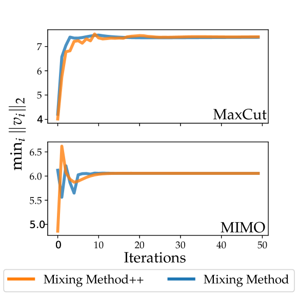
Figure 1. The minimum norm of the columns of $V$ throughout iterations of Mixing Method and Mixing Method++ on the MaxCut and MIMO objectives.

Put simply, Assumption 4.1 states that the update rule will never yield $u_{i}$ with zero norm. We find that this assumption consistently holds in practice for both Mixing Method and Mixing Method++ applied over several objectives. In particular, we track the smallest value of $\|\sum_{j\neq i}c_{ij}v_{j}\|_{2}$ observed during the inner loop of Mixing Method and Mixing Method++, then plot these minimum norms throughout all iterations in Figure 1. As can be seen, Assumption 4.1 consistently holds for both MaxCut and MIMO objectives. Furthermore, if Assumption 4.1 does not hold, we can exploit the simple trick from (Erdogdu et al., 2018) in practice. Given this assumption, no further assumptions are required for the second normalization step provided that $0\leq\beta<1$, as summarized below.

Observation 4.1.

$w_{i}=\|u_{i}-\beta v_{i}\|_{2}\not=0$, whenever $0\leq\beta<1$.

Proof.

Based on upper and lower triangle inequality bounds and the fact that $u_{i}$ and $v_{i}$ are both in $S^{k-1}$, we get the inequality $1\leq\left\lVert\left(1+\beta\right)u_{i}-\beta v_{i}\right\rVert_{2}\leq 1+2\beta$. ∎

Our first technical lemma lower bounds the decrease in the objective over inner iterations of Algorithm 2.

Lemma 4.0.

Let $\hat{V},V$ be the next and previous iteration of Algorithm (2), respectively. We define $y_{i}=\|g_{i}\|_{2}$, where $g_{i}=-\sum_{j\neq i}c_{ij}v_{j}$. We then derive the following.

$$f(V)-f(\hat{V})\geq\frac{1-\beta}{1+\beta}\sum_{i=1}^{n}y_{i}\,\|v_{i}-\hat{v}_{i}\|_{2}^{2}.$$

Furthermore, $f$ is non-increasing whenever $0\leq\beta<1$.

Next, we lower bound the magnitude of the update from $V$ to $\hat{V}$ based on the objective residual, showing that the magnitude of our update will be large until we approach an optimum.

Lemma 4.0.

Under assumption 4.1, there exists positive constants $\gamma$ and $\zeta$ such that

$$\|V-\hat{V}\|_{F}^{2}\geq\big{(}\zeta-\gamma\,\|\Delta\|_{F}\big{)}\,(f(V)-f^{*}),$$

where $\Delta:=(D_{w}D_{y}+\beta D_{y})-(D_{w^{*}}D_{y^{*}}+\beta D_{y^{*}})$.

Finally, we upper bound the value of $\|\Delta\|^{2}_{2}$ with respect to the objective residual, which later enables the definition of a neighborhood for local linear convergence within Theorem 4.4.

Lemma 4.0.

Under Assumption 4.1, $\exists~{}\tau>0$ such that

$$\|(w+\beta\mathds{1})\odot y-(w^{*}+\beta\mathds{1})\odot y^{*}\|_{2}^{2}\leq\tau(f(V)-f^{*}).$$

Drawing upon these technical lemmas, we show Mixing Method++ converges linearly within a neighborhood of the optimum.

Theorem 4.4 (Local linear convergence).

Let $f^{\star}$ represent the optimal value of the objective function, and let $\delta$ be the non-degenerative lower-bound of Assumption 4.1. Define the neighborhood,

$$\mathcal{N}_{\star}:=\left\{V\in(S^{k-1})^{n}\,:\,\tau(f(V)-f^{\star})\leq\left(\tfrac{\zeta-\kappa}{\gamma}\right)^{2}\right\},$$

for some positive constant $\kappa$ and $\zeta$, $\tau$, and $\gamma$ as defined in Lemmas  4.2 and 4.3. If $~{}V\in\mathcal{N}_{\star}$, we then have:

$$f(\hat{V})-f^{\star}\leq\left(1-\rho\right)\,\left(f(V)-f^{\star}\right),$$

where $\rho\in(0,1]$. This result shows that Algorithm (2) converges linearly when $V\in\mathcal{N}_{\star}$.

5. Experimental Results

We test Mixing Method++ on three well-known applications of (1): MaxCut, MaxSAT, and MIMO signal detection. We use the same formulation in (Wang et al., 2017) to solve MaxCut and MaxSAT, while for MIMO we follow the experimental setup in (Liu et al., 2017). We implement Mixing Method++ in C with $\beta=0.8$. Each experiment is run on a single core in a homogeneous Linux cluster with 2.63 GHz CPU and 16 GB of RAM. We compare Mixing Method++ with wide variety of solvers depending on the application. For MaxCut, we compare with CGAL (Yurtsever et al., 2019), Sedumi (Sturm, 1999), SDPNAL+ (Yang et al., 2015), SDPLR (Burer and Monteiro, 2003), MoSeK (ApS, 2019), and Mixing Method (Wang et al., 2017). For MaxSAT, we compare with Mixing Method and Loandra (Berg et al., 2019). Lastly, for MIMO signal detection, we compare with Mixing Method.

We often report performance in terms of the objective residual, which is defined as the difference between objective values given by each solver and the lowest objective value achieved by any solver. More formally, let $\texttt{Obj}_{ij}$ be the value of the objective function given by optimizer $i$ on SDP instance $j$. Then, the objective residual of optimizer $i$ on instance $j$ is defined as $|\texttt{Obj}_{ij}-\mathop{\min}\limits_{i^{\prime}\in O}\texttt{Obj}_{i^{\prime}j}|$, where $O$ is the set of all solvers used on problem instance $j$.

5.1. MaxCut

Solver		# SI		MLOR		Acc. ($\times$)
Sedumi		60		-4.30		360.20
MoSeK		74		-3.24		348.37
SDPNAL+		52		-4.33		1316.35
CGAL		92		0.93		49.19
SDPLR		95		-2.89		9.14
Mixing Method		106		-2.80		5.26
Mixing Method++		111		-3.87		1

Table 1. Results on 203 MaxCut instances. SI stands for solved instances; MLOR stands for median(log(objective residual)). Mixing Method++ solved most instances efficiently with good precision.

The SDP relaxation of the MaxCut problem is given by

$$\underset{\|v_{i}\|=1,}{\mathrm{max}}\,\frac{1}{2}\sum_{ij}c_{ij}\left(\tfrac{1-v_{i}^{\top}v_{j}}{2}\right),$$

where $C$ is the adjacency matrix. Thus, we aim to minimize the following objective function:

$$f_{\text{MaxCut}}=\left\langle C,\tfrac{\mathds{1}_{n\times n}-V^{\top}V}{4}\right\rangle~{}~{}\text{s.t.}~{}~{}\|v_{i}\|_{2}=1~{}~{}\forall i,$$

where $V\in\mathbb{R}^{k\times n}$ and $\mathds{1}_{n\times n}$ is the $n\times n$ matrix of all $1$s. We consider the following benchmarks within our MaxCut experiments.

• Gset: 67 binary-valued matrices, produced by an autonomous, random graph generator. The dimension $n$ varies from $800$ to $10^{4}$.

• Dimacs10: 152 symmetric matrices with $n$ varying from $39$ to $50,912,018$ , chosen for the $10$-th Dimacs Implementation Challenge. We consider the 136 instances with dimension $n\leq 8\cdot 10^{6}$.

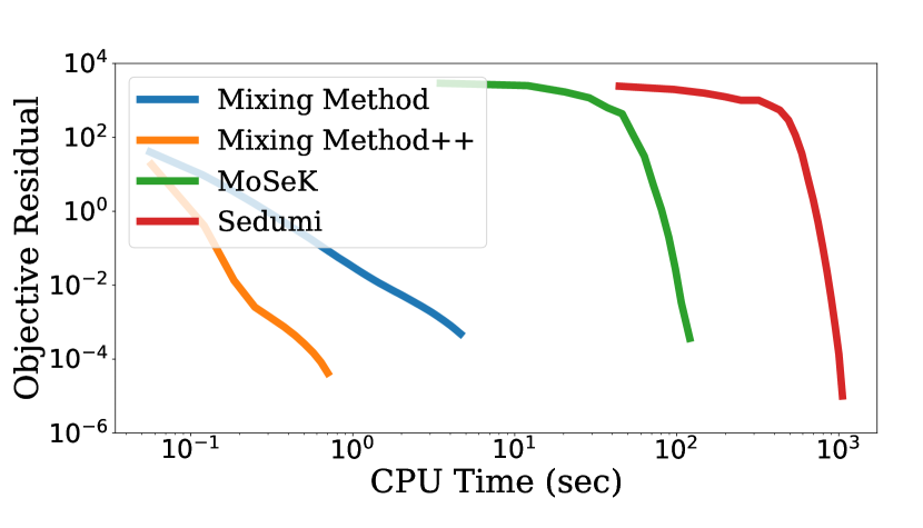
Figure 2. G40: $n=2000$, number of edges $=11766$. Mixing Method++ converges within $1$s while Mixing Method uses about $4$s. MoSeK and Sedumi need $10^{2}$ and $10^{3}$ seconds respectively to converge.

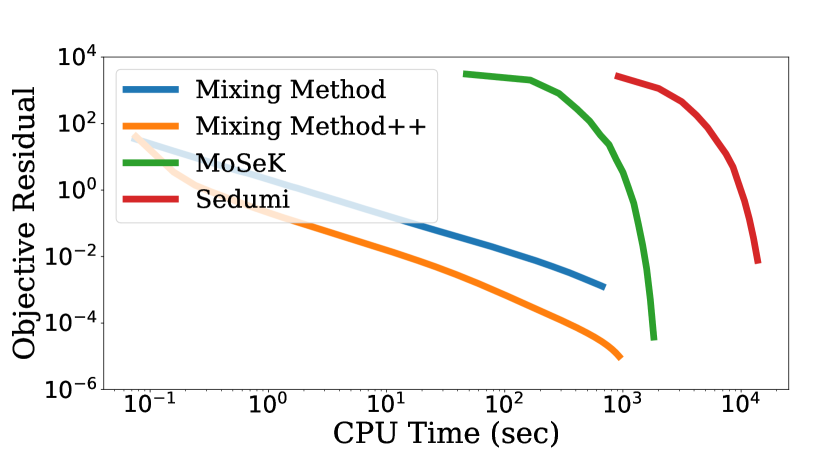
Figure 3. uk: $n=4824$, number of edges$=6837$. Consider the CPU time when each solver reaches objective residual $10^{-2}$. Mixing Method++ uses only 20s while Mixing Method needs 200s. MoSeK and Sedumi consume more than $10^{3}$ and $10^{4}$ seconds respectively.

Table 1 lists the number of solved instances, median logarithm of objective residual, and the pairwise acceleration ratio for different SDP solvers tested on MaxCut. In comparison to the other solvers, Mixing Method++ solves the most MaxCut instances (i.e., 111 of 203 total instances) within the imposed 24 hour time limit and provides a $5\times$ to $1316\times$ speedup. Moreover, the efficiency of Mixing Method++ does not harm its precision, which is evident in its median logarithm objective residual of $-3.87$. Such performance is preceded only by Sedumi $(-4.30)$ and SDPNAL+ $(-4.33)$, both of which are more than $300\times$ slower than Mixing Method++.

We also study two specific cases of MaxCut: G40 from Gset and uk from Dimacs10. In Figures 2 and 3, we plot objective residual with respect to CPU time of Mixing Method++ and other SDP solvers on the G40 and uk instances, respectively. In both MaxCut instances, Mixing Method++ converges significantly faster than other solvers that were considered.

5.2. MaxSAT

Methods		Avg. Approx. Ratio
Loandra		0.945
Mixing Method		0.975
Mixing Method++		0.977

Table 2. Results on MaxSAT. Mixing Method++ achieves the best approximation ratio with a time limit of 300s. 850 problems are tested in total. Problems are derived from crafted (331), random (454), and industrial domains (65).

Let $s_{ij}\in\{\pm 1,0\}$ be the sign of variable $i$ in clause $j$. The following problem provides an upper bound to the exact MaxSAT solution:

$$\underset{\|v_{i}\|=1,}{\mathrm{max}}\sum_{j=1}^{m}\left(1-\tfrac{\|Vs_{j}\|^{2}-(|s_{j}|-1)^{2}}{4|s_{j}|}\right),\vspace{-0.05cm}$$

where $s_{j}=[s_{1j},...,s_{nj}]^{\top}$. Therefore, the MaxSAT SDP relaxation can then be solved by minimizing the following, related objective:

$$f_{\text{MaxSAT}}=\left\langle C,{V^{\top}V}\right\rangle~{}~{}\text{s.t.}~{}~{}\|v_{i}\|_{2}=1~{}~{}\forall i,$$

where $V\in\mathbb{R}^{k\times n}$ and $C=\sum_{j=1}^{m}\frac{s_{j}s_{j}^{\top}}{4|s_{j}|}$.

We consider 850 problem instances from the 2016-2019 MaxSAT competition. Each instance is categorized as random, crafted or industrial. We evaluate Mixing Method++ as a partial MaxSAT solver and compare its performance to that of the Mixing Method and Loandra; the latter was the best partial solver in the 2019 MaxSAT competition. The best solution given by all solvers is used as ground truth when the optimal solution is not known.

The average approximation ratio of each solver across all MaxSAT instances is shown in Table 2. Mixing Method++ achieves the best average approximation ratio. We also consider two specific MaxSat instances: s3v90c800-6 from the random track and from the industrial track wb.4m8s4.dimacs.filtered. In Figures 4 and 5, we plot both the objective residual and the cost (i.e., the number of unsatisfied clauses) with respect to CPU time for s3v90c800-6 and wb.4m8s4.dimacs.filtered instances, respectively. Mixing Method++ converges faster than Mixing Method in both cases and returns the best solution on the s3v90c800-6 instance. Although Loandra provides the best solution to wb.4m8s4.dimacs.filtered quickly, Mixing Method++ still outperforms Mixing Method significantly.

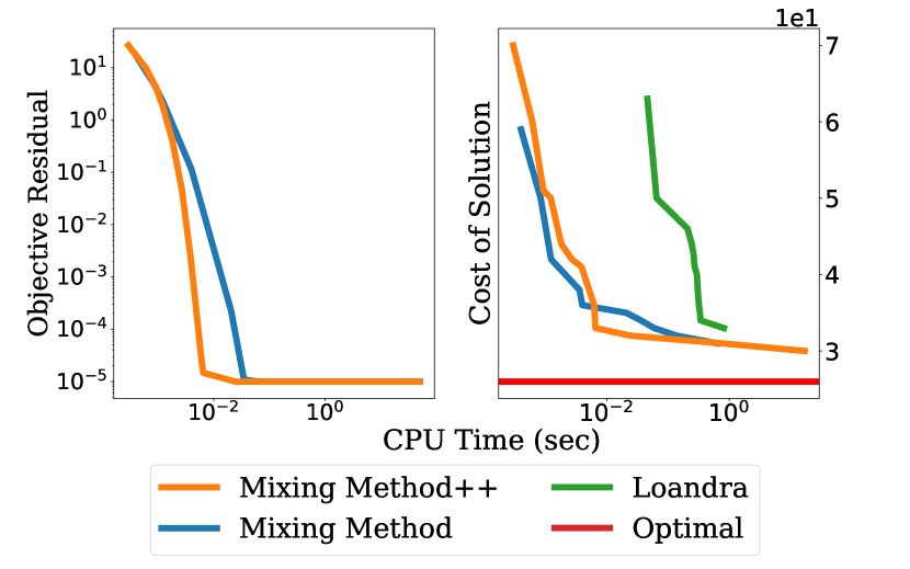
Figure 4. s3v90c800-6.cnf ($n=90$, $m=800$). Mixing Method++ not only converges faster than Mixing Method, but provides better solution (30) compared to Mixing Method (31) and Loandra (33). The optimal solution has cost 26.

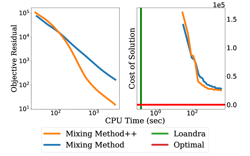
Figure 5. wb_4m8s4_dimacs_filtered.cnf ($n=463,080$, $m=1,759,150$). Loandra reaches optimal (230) in 1 sec, while Mixing Method and Mixing Method++ return a solution with cost $28,306$ and $25,210$ respectively in 1 hour.

5.3. MIMO

The MIMO signal detection setting is defined as follows:

$$\operatorname*{arg\,min}\limits_{x\in\mathcal{S}}\|y-Hx\|_{2}^{2},$$

where $y\in\mathbb{R}^{m}$ is the signal vector, $H\in\mathbb{R}^{m\times n}$ is the channel matrix, and $x\in\mathcal{S}$ is the transmitted signal. It is assumed that $y=Hx+v$, where $v$ is a noise vector. For our experiments, we consider the constellation $\{\pm 1\}$, which yields $\mathcal{S}=\{\pm 1\}^{n}$. The MIMO SDP relaxation can then be solved by minimizing the following objective.

$$f_{\text{MIMO}}=\langle C,V^{T}V\rangle~{}~{}\text{s.t.}~{}~{}\|v_{i}\|_{2}=1~{}~{}\forall i,$$

where $V\in\mathbb{R}^{k\times(n+1)}$ and $C=\begin{bmatrix}H^{T}H&-H^{T}y\\ -y^{T}H&y^{T}y\end{bmatrix}$.

We compare Mixing Method++ to Mixing Method on several simulated instances of the MIMO SDP objective. $H$ is sampled from a standard normal distribution, $x$ is sampled from $\{\pm 1\}$, and $v$ is sampled from a centered normal distribution with variance $\sigma_{v}^{2}$. Experiments are performed for numerous settings of $\sigma_{v}^{2}$ determined by the signal-to-noise ratio (SNR) (i.e., $\sigma_{v}^{2}=\frac{mn}{\text{SNR}}$). We perform tests with $\text{SNR}\in\{8,16\}$ and problem sizes $(m,n)\in\{(16,16),(32,32),(64,32)\}$. We plot the objective residual achieved by both Mixing Method and Mixing Method++ on MIMO instances with respect to CPU time in Figure 6. As can be seen, Mixing Method++ matches or exceeds the performance of the Mixing Method in all experimental settings.

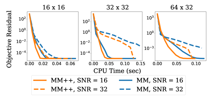
Figure 6. Convergence comparison of Mixing Method++ and Mixing Method on MIMO signal detection problems with different SNRs. The size of the channel matrix is listed above each subplot.

5.4. The Effect of Sparsity

We empirically observe that Mixing Method++ achieves different levels of acceleration based on the sparsity of $C$. To further understand the impact of sparsity on the performance of Mixing Method++, we compare Mixing Method++ to Mixing Method for objectives with different sparsity levels. In particular, we construct a MaxCut objective for a graph with 500 nodes and consider adjacency matrices with three different sparsity levels: $0.8$, $0.5$, and $0.2$. In Figure 7, we plot the objective residual of both Mixing Method and Mixing Method++ on these problem instances. As can be seen, the acceleration achieved by Mixing Method++ is more significant when $C$ is sparse. Furthermore, decreasing the value of $\beta$ improves the performance of Mixing Method++ on MaxCut instances when $C$ is dense.

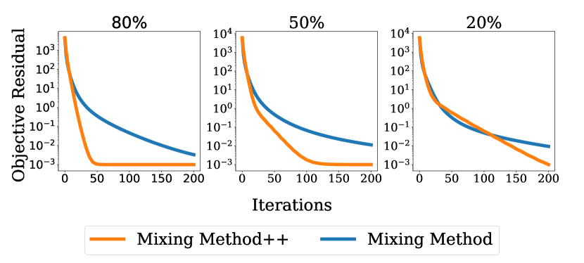
Figure 7. Convergence comparison of Mixing Method++ (blue line) with $\beta=0.8$ and Mixing Method (orange line) on 500-node MaxCut problem instances with different sparsity levels.

5.5. Adaptive Momentum

We observe that Mixing Method sometimes decreases the objective residual faster than Mixing Method++ during early stage iterations. Inspired by this observation and previous work on adaptive momentum schedules (O’donoghue and Candes, 2015; Chen et al., 2019; Wang et al., 2020), we explore whether dynamically adjusting the value of $\beta$ between iterations can further improve the performance of Mixing Method++. We propose the following momentum schedule:

$$\beta_{t}=\beta\left(1-\exp(-\alpha t/T)\right),$$

where $\beta=0.8$ is the default momentum, $t$ is the current iteration, $T$ is the total number of iterations, and $\alpha$ is a constant such that $\exp(-\alpha)\approx 0$. Intuitively, this schedule begins with a low momentum value, which quickly increases to $\beta=0.8$, thus forming a warm-up schedule for the momentum. As shown in Figure 8, this schedule improves the convergence speed of Mixing Method++.

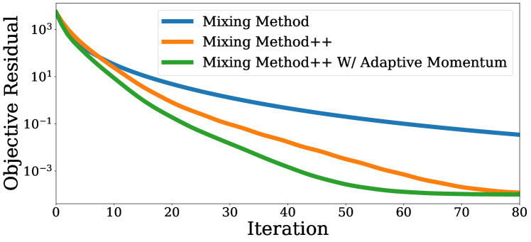
Figure 8. Comparison of Mixing Method (orange line), Mixing Method++ with fixed momentum $\beta=0.8$ (blue line), Mixing Method++ with an increasing Scheduled Momentum from $0$ to $0.8$ (green line) in terms of the objective cost per iteration.

6. Local linear convergence

We now give detailed proof of Theorem 4.4. Let $g_{i}$ be the linear combination in step 4 of Algorithm 1, before projecting onto the unit sphere:

$$\begin{split}g_{i}&=\sum_{j<i}c_{ij}\hat{v}_{j}+\sum_{j>i}c_{ij}v_{j}.\end{split}$$

We also define $y_{i}=\|g_{i}\|_{2}$ and $f(V)\triangleq\langle C,V^{T}V\rangle$ as the objective value for some viable solution $V$. Therefore, step 4 of Algorithm 1 can be expressed as: $y_{i}u_{i}=-g_{i}$. Thus, the changes presented in the Algorithm 2 can be written as the combination of 4 and the momentum, in step 5:

$$\begin{split}u_{i}=-\frac{g_{i}}{y_{i}},\hskip 10.0pt\text{ and }\hskip 10.0pt\hat{v}_{i}=\frac{\left(1+\beta\right)u_{i}-\beta v_{i}}{w_{i}},\end{split}$$

where $w_{i}=\left\lVert\left(1+\beta\right)u_{i}-\beta v_{i}\right\rVert_{2}$. This leads to the following one line relation,

(6) $$w_{i}y_{i}\hat{v}_{i}=-\left(1+\beta\right)g_{i}-\beta y_{i}v_{i},~{}\forall i\in[n].$$

Herein, the matrices $V$ and $\hat{V}$ refer to the current and the end state of the inner iteration in algorithm 2. For each $i\in[n]$, we define the family of maps $Z_{i}:(S^{k-1})^{n}\to(S^{k-1})^{n}$ as follows

(7) $$Z_{i}(V)\,e_{j}=\begin{cases}\hat{v}_{j},\hskip 10.0pt\text{if $j<i$}\\ v_{j},\hskip 10.0pt\text{if $j\geq i$},\end{cases}$$

where $\{e_{j}\}$ is the canonical basis in $\mathbb{R}^{n}$. It is trivial to see that $Z_{i}(V)$ corresponds to the matrix in the inner cycle before updating $v_{i}$ to $\hat{v}_{i}$. Thus, only the vector $v_{i}$ has been changed from $Z_{i}(V)$ to $Z_{i+1}(V)$. Also notice that $Z_{n+1}(V)$ corresponds to the end of the inner cycle, i.e., $Z_{n+1}(V)=\hat{V}$.

Matrix Representation

The transition from the state $v_{i}$ to $\hat{v}_{i}$ is expressed in the relation (6), then for any $i\in[n]$ in each inner cycle we have,

(8) $$\begin{split}\left(1+\beta\right)\sum_{j<i}c_{ij}\hat{v}_{j}+w_{i}y_{i}\hat{v}_{i}=-\left(1+\beta\right)\sum_{j>i}c_{ij}v_{j}-\beta y_{i}v_{i}.\end{split}$$

Let $L$ be the strictly lower triangular matrix of $C$ so (8) leads us to the representation:

(9) $$\left(\left(1+\beta\right)L+D_{w}D_{y}\right)\,\hat{V}^{\top}=-\left(\left(1+\beta\right)L^{\top}+\beta D_{y}\right)\,V^{\top}.$$

Proof of Lemma 4.1

Let $\beta$ be in $[0,1]$. When fixing all the others variables, $f$ with respect to $v_{i}$ is given by

$$\langle C,V^{\top}V\rangle=2v_{i}^{\top}\big{(}\sum_{j}c_{ij}v_{j}\big{)}+\text{constant}.$$

Since only $v_{i}$ is changed, during the $i$th coordinate-wise updating, the only part of the objective that will change is $2v_{i}^{\top}g_{i}$. That is,

$$f(Z_{i}(V))-f(Z_{i+1}(V))=2g_{i}^{\top}\left(v_{i}-\hat{v}_{i}\right).$$

The updating rule of algorithm 2 is given by the recursion (6), so using this into the above equation yields

$$\begin{split}f(Z_{i}(V))-f(Z_{i+1}(V))&=\frac{2y_{i}\,(w_{i}-\beta)}{1+\beta}(1-v_{i}^{\top}\hat{v}_{i}),\\ &=\frac{y_{i}\,(w_{i}-\beta)}{1+\beta}\|v_{i}-\hat{v}_{i}\|_{2}^{2}.\end{split}$$

From observation 4.1, we have $w_{i}-\beta\geq 1-\beta$. Thus,

$$\begin{split}f(Z_{i}(V))-f(Z_{i+1}(V))\geq y_{i}\,\frac{1-\beta}{1+\beta}\|v_{i}-\hat{v}_{i}\|_{2}^{2}.\end{split}$$

Adding over all the $i$, leads us to the desired conclusion

$$\begin{split}f(V)-f(\hat{V})&=\sum_{i=1}^{n}\,f(Z_{i}(V))-f(Z_{i+1}(V))\\ &\geq\frac{1-\beta}{1+\beta}\sum_{i=1}^{n}y_{i}\,\|v_{i}-\hat{v}_{i}\|_{2}^{2}.\end{split}$$

The following observation will be useful later on.

Observation 6.1.

For all $i\in[n]$, $w_{i}^{*}=1$

Proof.

Since $v^{*}_{i}$ is a fixed point, using this fact in Eq. (6) yields $(w^{*}_{i}+\beta)v_{i}^{*}=u_{i}^{*}$. Taking the norm, $w_{i}^{*}+\beta=1+\beta$, since $u^{*}_{i}$ and $v^{*}_{i}$ are in the unit sphere. ∎

Let $S$ be defined as $\left(1+\beta\right)C+D_{w}D_{y}+\beta D_{y}$ and let $S^{*}$ be $\left(1+\beta\right)C+D_{w^{*}}D_{y^{*}}+\beta D_{y^{*}}$; namely, the corresponding value of $S$ when $V$ is optimal in the optimization (3). We have the following observation.

Observation 6.2.

$S^{*}$ is PSD.

Proof.

By observation 6.1 we have $w^{*}_{i}=1$, so

$$S^{*}=\left(1+\beta\right)C+D_{w^{*}}D_{y^{*}}+\beta D_{y^{*}}=\left(1+\beta\right)\left(C+D_{y}^{*}\right),$$

where according to lemma 3.12, and since $V$ is optimal, it follows that $\frac{S^{*}}{1+\beta}\succeq 0$, hence $S^{*}\succeq 0$. ∎

Proof of Lemma 4.2

By (9), we have

$$\hat{V}=\,-V\left(\left(1+\beta\right)L+\beta D_{y}\right)\left(\left(1+\beta\right)L^{\top}+D_{w}D_{y}\right)^{-1}.$$

This leads to

$$\begin{split}V-\hat{V}=&V(\left(1+\beta\right)C+D_{w}D_{y}+\beta D_{y})\\ &(\left(1+\beta\right)L^{\top}+D_{w}D_{y})^{-1}\\ =&VS\underbrace{(\left(1+\beta\right)L^{\top}+D_{w}D_{y})^{-1}}_{R},\end{split}$$

Using the definition $\Delta\triangleq(D_{w}D_{y}+\beta D_{y})-(D_{w^{*}}D_{y^{*}}+\beta D_{y^{*}})$, and the fact that $S=S^{*}+\Delta$ in the previous equation, we get

(10) $$\begin{split}\|V-\hat{V}\|_{F}^{2}&\geq\|VS^{*}R\|_{F}^{2}+2\text{tr}\big{(}V^{\top}VS^{*}RR^{\top}\Delta\big{)}.\end{split}$$

We claim that

$$\|(w+\beta\mathds{1})\odot y-(w^{*}+\beta\mathds{1})\odot y^{*}\|_{2}I_{n}+\Delta\succeq 0.$$

To see this, first notice $D_{w}D_{y}+\beta D_{y}=D_{(w+\beta\mathds{1})\odot y}$. Thus,

$$\Delta=D_{(w+\beta\mathds{1})\odot y}-D_{(w^{*}+\beta\mathds{1})\odot y^{*}}.$$

Besides,

$$\|(w+\beta\mathds{1})\odot y-(w^{*}+\beta\mathds{1})\odot y^{*}\|_{2}=\|\Delta\|_{F}.$$

So the claim follows since $\beta\geq 0$ and termwise

$$\begin{split}\|\Delta\|_{F}+\Delta_{i}\geq|\Delta_{i}|+\Delta_{i}\geq 0.\end{split}$$

Now, for the first part in (10), we get

$$\begin{split}\|VS^{*}R\|_{F}^{2}&=\text{tr}(\underbrace{{S^{*}}^{\top}}_{\succeq 0}\underbrace{V^{\top}V}_{\succeq 0}\underbrace{S^{*}}_{\succeq 0}\underbrace{RR^{\top}}_{\succeq 0})\\ &\geq\sigma_{\min}^{2}(R)\sigma_{\texttt{nnz}}(S^{*})\text{tr}(V^{T}VS^{*}).\end{split}$$

For the second in (10), we get

$$\begin{split}\text{tr}\big{(}V^{\top}VS^{*}RR^{\top}\Delta\big{)}&\geq-\|\Delta\|_{F}\operatorname*{\text{Tr}}\big{(}V^{\top}VS^{*}RR^{\top}\big{)}\\ &\geq-\|\Delta\|_{F}\,\sigma_{\max}^{2}(R)\text{tr}\big{(}V^{\top}VS^{*}\big{)},\end{split}$$

this last inequality is given by our previous claim, the fact that $S^{*}\succeq 0$ (observation 6.2) and

$$\begin{split}\operatorname*{\text{Tr}}(V^{\top}VS^{*}RR^{\top})&=\operatorname*{\text{Tr}}(V^{\top}VS^{*}\underbrace{UD^{2}U^{\top}}_{RR^{\top}})=\operatorname*{\text{Tr}}(V^{\top}VS^{*}D^{2})\\ &\leq\sigma^{2}_{\max}(R)\,\operatorname*{\text{Tr}}(V^{\top}VS^{*}).\end{split}$$

Using the lower bounds in (10) gives us

$$\begin{split}\|V&-\hat{V}\|_{F}^{2}\geq\big{(}\sigma_{\min}^{2}(R)\sigma_{\texttt{nnz}}(S^{*})-2\|\Delta\|_{F}\sigma_{\max}^{2}(R)\big{)}\text{tr}\big{(}V^{\top}VS^{*}\big{)}.\end{split}$$

To conclude, the term

$$\begin{split}\operatorname*{\text{Tr}}(V^{\top}VS^{*})&=\operatorname*{\text{Tr}}(V^{\top}VC)-\operatorname*{\text{Tr}}(-V^{\top}VD_{y^{*}})=f(V)-\operatorname*{\text{Tr}}(-V^{\top}VD_{y^{*}})\\ &\stackrel{{\scriptstyle i)}}{{=}}f(V)+\sum\limits_{i}\underbrace{\langle v_{i},v_{i}\rangle}_{=1}\cdot y^{*}_{i}=f(V)+\langle\mathds{1},y^{*}\rangle\\ &\stackrel{{\scriptstyle ii)}}{{\geq}}f(V)-f^{*}.\end{split}$$

where $i)$ follows from the fact that $D_{y^{*}}$ is diagonal. To understand $ii)$, consider the dual to the diagonally constrained SDP problem (1) (i.e., see Lemma 3.12 of (Wang et al., 2017) for more details):

(11) $$\max\limits_{y}-\langle\mathds{1},y\rangle,~{}\text{such that }C+D_{y}\succeq 0$$

We know that $C+D_{y^{*}}=\frac{S^{*}}{1+\beta}\succeq 0$ from Observation 6.2. Therefore, $y^{*}$ is a feasible solution to the dual problem (11), revealing that $f^{*}\geq-\langle\mathds{1},y^{*}\rangle$. This fact allows us to derive the inequality given by $ii)$. Then, if we define $\zeta=\sigma^{2}_{\min}(R)\sigma_{nnz}(S^{*})$ and $\gamma=2\sigma^{2}_{\max}(R)$ with $\sigma_{\min}(R)=1/(w\odot y)_{\max}$ and $\sigma_{\max}(R)=1/(w\odot y)_{\min}$, we arrive at the final result:

$$\|V-\hat{V}\|^{2}_{F}\geq\left(\zeta-\gamma\|\Delta\|_{F}\right)(f(V)-f^{\star})$$

It should be noted that both $\zeta$ and $\gamma$ are strictly positive constants because $R$ is defined as an invertible matrix and, therefore, has all non-zero eigenvalues.

Proof of Lemma 4.3

Recall that $\Delta_{i}=(w_{i}+\beta)y_{i}-(w_{i}^{\star}+\beta)y_{i}^{\star}$. We can unroll the value of $\Delta_{i}\hat{v}_{i}$ into the following expression:

(12) $$\big{(}(w_{i}y_{i}-w_{i}^{*}y_{i}^{*})+\beta(y_{i}-y_{i}^{*})\big{)}\,\hat{v_{i}}$$

Then, we derive the following equality from (6):

(13) $$\begin{split}w_{i}y_{i}\hat{v_{i}}&=-\left(1+\beta\right)g_{i}-\beta y_{i}v_{i}\\ &=-\left(1+\beta\right)Z_{i}c_{i}-\beta y_{i}v_{i}\end{split}$$

where we denote $Z_{i}=Z_{i}(V)$ for brevity and $c_{i}$ as the $i$th column of $C$. We denote $s_{i}^{*}=\left(1+\beta\right)c_{i}+w_{i}^{*}y_{i}^{*}e_{i}+\beta y_{i}^{*}e_{i}$. By adding (12) to both sides of (13), we arrive at the following, expanded version of the update rule in (6).

(14) $$\begin{split}&w_{i}y_{i}\hat{v_{i}}-w_{i}^{*}y_{i}^{*}\hat{v_{i}}+\beta y_{i}\hat{v_{i}}-\beta y_{i}^{*}\hat{v_{i}}\\ &=-\left(1+\beta\right)Z_{i}c_{i}-\beta y_{i}v_{i}-w_{i}^{*}y_{i}^{*}\hat{v_{i}}+\beta y_{i}\hat{v_{i}}-\beta y_{i}^{*}\hat{v_{i}}\\ &\stackrel{{\scriptstyle i)}}{{=}}-Z_{i}s_{i}^{*}+\big{(}w_{i}^{*}y_{i}^{*}-\beta(y_{i}-y_{i}^{*})\big{)}(v_{i}-\hat{v_{i}}).\end{split}$$

where $i)$ follows from the definition of $s_{i}^{\star}$ and the fact that $Z_{i}e_{i}=v_{i}$. By combining Assumption 4.1 and Lemma 4.1, it is known that

(15) $$f(V)-f^{*}\geq\frac{1-\beta}{1+\beta}\,\delta\,\|v_{i}-\hat{v_{i}}\|_{2}^{2}.$$

Besides,

(16) $$\begin{split}f(V)-f^{*}&\geq f(Z_{i})-f^{*}=\operatorname*{\text{Tr}}(Z_{i}^{\top}Z_{i}S^{*})\\ &\geq\sigma^{-1}_{\max}(S^{*})\|Z_{i}S^{*}\|_{F}^{2}\geq\sigma^{-1}_{\max}(S^{*})\|Z_{i}s_{i}^{*}\|_{2}^{2}\end{split}$$

Therefore, based on (15) and (16), it is known that $\|Z_{i}s_{i}^{\star}\|_{2}^{2}$ and $\|v_{i}-\hat{v}_{i}\|^{2}_{2}$ are both upper bounded by a positive factor of $f(V)-f^{\star}$. The inner product of (12) with itself to yields:

$$\Delta_{i}^{2} \stackrel{{\scriptstyle i)}}{{=}}\big{(}(w_{i}y_{i}-w_{i}^{*}y_{i}^{*})+\beta(y_{i}-y_{i}^{*})\big{)}^{2}$$

$$\stackrel{{\scriptstyle ii)}}{{\leq}}2\|Z_{i}s_{i}^{*}\|^{2}+2(y^{*}_{i}-\beta y_{i})^{2}\|v_{i}-\hat{v_{i}}\|^{2}$$

$$=2\|Z_{i}s_{i}^{*}\|^{2}+2({y^{*}_{i}}^{2}-2\beta y_{i}^{*}y_{i}+{y_{i}}^{2})\,\|v_{i}-\hat{v_{i}}\|^{2}$$

where $i)$ follows from the fact that $\hat{v}_{i}$ is a unit vector and $ii)$ follows from combining observation 6.1 with (14). Next, we have:

$$\|(w+\beta\mathds{1})\odot y-(w^{*}+\beta\mathds{1})\odot y^{*}\|_{2}^{2}=\|\Delta\|_{F}^{2}=\sum\limits_{i=1}^{n}\Delta_{i}^{2}.$$

We combine this expression with the upper bounds for $\|Z_{i}s_{i}^{\star}\|^{2}_{2}$ and $\|v_{i}-\hat{v}_{i}\|^{2}_{2}$ derived in (15) and (16) to arrive at the final result, where $\tau$ is defined as some positive constant:

$$\|(w+\beta\mathds{1})\odot y-(w^{*}+\beta\mathds{1})\odot y^{*}\|_{2}^{2}\leq\tau(f(V)-f^{*})$$

Proof of Theorem 4.4

Based on Lemma 4.3, a neighborhood can be selected around the optimum such that the value of $f(V)-f^{\star}$ is sufficiently small. We define this neighborhood through the selection of a positive constant $\kappa$ such that the following inequality holds, where $\tau$ is defined in Lemma 4.3:

(17) $$\left(\frac{\zeta-\kappa}{\gamma}\right)^{2}\geq\tau\left(f(V)-f^{\star}\right)$$

Within this expression, $\zeta$ and $\gamma$ are both defined in Lemma 4.2. Because $\zeta$ and $\gamma$ are both strictly positive (i.e., see Lemma 4.2), $\left(\frac{\zeta-\kappa}{\gamma}\right)$ is known to be strictly positive so long as $\kappa\in[0,\zeta)$. Therefore, there always exists a value of $\kappa$ such that (17) will be true within a sufficiently small neighborhood around the optimum. We combine (17) with the inequality from Lemma 4.3 to yield the following:

$$\left(\frac{\zeta-\kappa}{\gamma}\right)^{2}\geq\tau(f(V)-f^{*})\geq\|\Delta\|_{F}^{2},$$

Then, because $\left(\frac{\zeta-\kappa}{\gamma}\right)$ is strictly positive, we can manipulate the above expression to yield the following:

(18) $$\zeta-\gamma\|\Delta\|_{F}\geq\kappa.$$

The above inequality holds for all successive iterations of Algorithm 2. Then, based on the combination of Lemma 4.1 and assumption 4.1, $f(V)-f(\hat{V})\geq\delta\frac{1-\beta}{1+\beta}\|V-\hat{V}\|_{F}^{2}$, and thus

$$\begin{split}f(V)-f(\hat{V})&\geq\delta\frac{1-\beta}{1+\beta}\|V-\hat{V}\|_{F}^{2}\\ &\stackrel{{\scriptstyle i)}}{{\geq}}\delta\frac{1-\beta}{1+\beta}\kappa(f(V)-f^{*})\end{split}$$

where $i)$ is derived by combining (18) and Lemma 4.2. This expression in turn implies the following.

$$\left(1-\delta\kappa\frac{1-\beta}{1+\beta}\right)(f(V)-f^{*})\geq f(\hat{V})-f^{*}.$$

thus giving us the desired linear convergence. By substituting $\rho=\delta\kappa\frac{1-\beta}{1+\beta}$, we arrive at the final result.

7. Convergence to first-order critical point

Mixing method++ not only has local linear convergence, but it always converges to a first-order critical point, per following Theorem:

Theorem 7.1.

Let $V^{\ell}=Z_{n+1}^{\ell}(V)$, see definition (7), for all $\ell\in\mathbb{N}$; i.e., the collection of points generated by Mixing Method++ after finishing the inner loop. Then, under the assumption 4.1, $\{V^{\ell}\}_{\ell}$ converges to a limit point $\bar{V}$ and the Riemannian gradient at $\bar{V}$ is zero (Mixing Method++ converges to a first-order critical point).

Proof.

For $\beta$ in $[0,1)$ we know by lemma 4.1 that the objective function is decreasing. Besides, $(S^{k-1})^{n}$ is compact, indeed limit point compact, so there exists a limit point $\bar{V}$ such that $f(\bar{V})=\lim_{k}f(V^{k})$ by continuity of $f$. It is clear that $\bar{V}$ is a fixed point in relation (9), so

(19) $$\bar{V}C=-\frac{\bar{V}D_{(\bar{w}+\beta\mathds{1})\odot\bar{y}}}{1+\beta}.$$

Since the constraint set is a product of spheres, its corresponding tangent space (henceforth denoted by the letter $\mathrm{T}$) at the point $\bar{V}$ is given by the product of tangent spaces of $S^{k-1}$; namely

(20) $$\mathrm{T}_{\bar{V}}\left(S^{k-1}\right)^{n}=\prod_{j=1}^{n}\mathrm{T}_{\bar{v_{j}}}\,\left(S^{k-1}\right),$$

where $\bar{v}_{j}$ is the $j$th column of $\bar{V}$.

The above result gives us a way to characterize the tangent space. To this end, it is actually enough to work with the tangent space of $S^{k-1}$.

By definition, for any $v_{j}$, the vector $\dot{v}_{j}\in\mathbb{R}^{k}$ is in the tangent space of $S^{k-1}$ if and only if there exists a curve $\varphi:I\to S^{k-1}$ such that $\varphi(0)=v_{j}$ and $\dot{\varphi}(0)=\dot{v}_{j}$, where $\dot{\varphi}$ is the derivative of $\varphi$. Then $\varphi(t)\in S^{k-1}$ if satisfies $\langle\varphi(t),\varphi(t)\rangle=1$ for all $t\in I$. Differentiating on both sides leads us to $0=\langle\dot{\varphi}(t),\varphi(t)\rangle+\langle\varphi(t),\dot{\varphi}(t)\rangle$. Evaluating at $t=0$, we get

$$2\langle\dot{v}_{j},v_{j}\rangle=0,$$

thus $\{\dot{v}_{j}\in\mathbb{R}^{k}:\langle\dot{v}_{j},v_{j}\rangle=0\}\subseteq\mathrm{T}_{v_{j}}S^{k-1}$, since both subspaces are of the same dimension, $\{\dot{v}_{j}\in\mathbb{R}^{k}:\langle\dot{v}_{j},v_{j}\rangle=0\}=\mathrm{T}_{v_{j}}S^{k-1}$.

Now by (20) and the previous analysis, we finally arrive to the characterization of the tangent space; namely

$$\mathrm{T}_{\bar{V}}\left(S^{k-1}\right)^{n}=\left\{\dot{\bar{V}}\in\mathbb{R}^{k\times n}:\langle\dot{\bar{v}}_{j},\bar{v}_{j}\rangle=0\hskip 5.0pt\forall j\in[n]\,\right\},$$

and $\dot{\bar{v}}_{j}$ ($v_{j}$) corresponds to the $j$th column of $\dot{\bar{V}}$ ($\bar{V}$), respectively.

Let $\mathrm{P}^{\perp}:\mathbb{R}^{k\times n}\to\mathrm{T}_{\bar{V}}\left(S^{k-1}\right)^{n}$ be the projector operator from the euclidean space to the tangent space at $\bar{V}$, defined for any $W\in\mathbb{R}^{k\times n}$ as follows,

$$W\xrightarrow{\mathrm{P}^{\perp}}\begin{pmatrix}w_{1}-\langle\bar{v}_{1},w_{1}\rangle\bar{v}_{1}&\ldots&w_{n}-\langle\bar{v}_{n},w_{n}\rangle\bar{v}_{n}\end{pmatrix}.$$

Let the Riemannian gradient of $f$ denoted by $\mathrm{grad}f(\cdot)$, and the gradient of $f$ defined in the entire euclidean domain as $\nabla f(\cdot)$. Using tools from matrix manifold the Riemannian gradient is given by

$$\mathrm{grad}f(\bar{V})=\mathrm{P}^{\perp}(\nabla f(\bar{V})).$$

It is easy to see that $\nabla f(\bar{V})=2\bar{V}C$, and by relation (19), this yields us to the equivalent version $\nabla f(\bar{V})=-\frac{2}{1+\beta}\bar{V}D_{(\bar{w}+\beta\mathds{1})\odot\bar{y}}$.

Finally, $\left(\nabla f(\bar{V})\right)_{j}=-\frac{2}{1+\beta}(w_{j}y_{j}+\beta y_{j})\bar{v}_{j}$, $\forall j\in[n]$ and by definition of the projection map we get

$$\begin{split}\left(\mathrm{P}^{\perp}(\nabla f(\bar{V}))\right)_{j}=\frac{2}{1+\beta}(w_{j}y_{j}+\beta y_{j})(-\bar{v}_{j}+\bar{v}_{j})=0.\end{split}$$

So, we have $\left(\mathrm{P}^{\perp}(\nabla f(\bar{V})\right)_{j}=0$, for all coordinates $j\in[n]$, and thus

$$\mathrm{grad}f(\bar{V})=\mathrm{P}^{\perp}(\nabla f(\bar{V}))=0.$$

∎

8. Conclusion and Future Directions

We present a novel approach, Mixing Method++, to solve diagonally constrained SDPs. Mixing Method++ inherits the simplicity—and non-trivially preserves theoretical guarantees from—its predecessor. In practice, it yields not only faster convergence on nearly all tested instances, but also improvements in solution quality. Mixing Method++ adds one addition hyperparameter $\beta$ for which we provide a theoretical upper bound (i.e., $\beta<1$). Using $\beta=0.8$ experimentally leads to a robust algorithm, which outperforms Mixing Method and numerous other state-of-the-art SDP solvers. Theoretically validating the experimental acceleration provided by Mixing Method++ is still an open problem, which could potentially be handled with the help of Lyapunov Analysis (Wilson et al., 2016; Jin et al., 2018).

- (1)
- Abbe (2018) E. Abbe. 2018. Community Detection and Stochastic Block Models. Foundations and Trends® in Communications and Information Theory 14, 1-2 (2018), 1–162.
- Alizadeh et al. (1997) Farid Alizadeh, Jean-Pierre A Haeberly, and Michael L Overton. 1997. Complementarity and nondegeneracy in semidefinite programming. Mathematical programming 77, 1 (1997), 111–128.
- ApS (2019) Mosek ApS. 2019. Mosek optimization toolbox for MATLAB. User’s Guide and Reference Manual, version 4 (2019).
- Assran and Rabbat (2020) M. Assran and M. Rabbat. 2020. On the Convergence of Nesterov’s Accelerated Gradient Method in Stochastic Settings. arXiv preprint arXiv:2002.12414 (2020).
- Barahona et al. (1988) F. Barahona, M. Grötschel, M. Jünger, and G. Reinelt. 1988. An application of combinatorial optimization to statistical physics and circuit layout design. Operations Research 36, 3 (1988), 493–513.
- Barvinok (1995) Alexander I. Barvinok. 1995. Problems of distance geometry and convex properties of quadratic maps. Discrete & Computational Geometry 13, 2 (1995), 189–202.
- Berg et al. (2019) Jeremias Berg, Emir Demirović, and Peter J. Stuckey. 2019. Core-Boosted Linear Search for Incomplete MaxSAT. In Integration of Constraint Programming, Artificial Intelligence, and Operations Research, Louis-Martin Rousseau and Kostas Stergiou (Eds.). Springer International Publishing, Cham, 39–56.
- Bhojanapalli et al. (2018) S. Bhojanapalli, N. Boumal, P. Jain, and P. Netrapalli. 2018. Smoothed analysis for low-rank solutions to semidefinite programs in quadratic penalty form. arXiv preprint arXiv:1803.00186 (2018).
- Bhojanapalli et al. (2016) Srinadh Bhojanapalli, Anastasios Kyrillidis, and Sujay Sanghavi. 2016. Dropping convexity for faster semi-definite optimization. In Conference on Learning Theory. 530–582.
- Boumal (2016) N. Boumal. 2016. Nonconvex phase synchronization. SIAM Journal on Optimization 26, 4 (2016), 2355–2377.
- Burer and Monteiro (2003) S. Burer and R. Monteiro. 2003. A nonlinear programming algorithm for solving semidefinite programs via low-rank factorization. Mathematical Programming 95, 2 (2003), 329–357.
- Chen et al. (2019) John Chen, Cameron Wolfe, Zhao Li, and Anastasios Kyrillidis. 2019. Demon: Momentum Decay for Improved Neural Network Training. arXiv preprint arXiv:1910.04952 (2019).
- Devolder et al. (2014) O. Devolder, F. Glineur, and Y. Nesterov. 2014. First-order methods of smooth convex optimization with inexact oracle. Mathematical Programming 146, 1-2 (2014), 37–75.
- Deza and Laurent (1994) M. Deza and M. Laurent. 1994. Applications of cut polyhedra - II. J. Comput. Appl. Math. 55, 2 (1994), 217–247.
- Erdogdu et al. (2018) Murat A. Erdogdu, Asuman Ozdaglar, Pablo A. Parrilo, and Nuri Denizcan Vanli. 2018. Convergence Rate of Block-Coordinate Maximization Burer-Monteiro Method for Solving Large SDPs. arXiv e-prints, Article arXiv:1807.04428 (July 2018), arXiv:1807.04428 pages. arXiv:1807.04428 [math.OC]
- Frieze and Jerrum (1995) Alan Frieze and Mark Jerrum. 1995. Improved approximation algorithms for MAX -CUT and MAX BISECTION. In International Conference on Integer Programming and Combinatorial Optimization. Springer, 1–13.
- Gärtner and Matousek (2012) B. Gärtner and J. Matousek. 2012. Approximation algorithms and semidefinite programming. Springer Science & Business Media.
- Ghadimi et al. (2015) E. Ghadimi, H. Feyzmahdavian, and M. Johansson. 2015. Global convergence of the heavy-ball method for convex optimization. In 2015 European control conference (ECC). IEEE, 310–315.
- Gieseke et al. (2013) F. Gieseke, T. Pahikkala, and C. Igel. 2013. Polynomial runtime bounds for fixed-rank unsupervised least-squares classification. In Asian Conference on Machine Learning. 62–71.
- Goemans and Williamson (1995) M. Goemans and D. Williamson. 1995. Improved approximation algorithms for maximum cut and satisfiability problems using semidefinite programming. Journal of the ACM (JACM) 42, 6 (1995), 1115–1145.
- Goemans and Williamson (2004) Michel X Goemans and David P Williamson. 2004. Approximation algorithms for MAX-3-CUT and other problems via complex semidefinite programming. J. Comput. System Sci. 68, 2 (2004), 442–470.
- Goto et al. (2019) Hayato Goto, Kosuke Tatsumura, and Alexander R Dixon. 2019. Combinatorial optimization by simulating adiabatic bifurcat‘ions in nonlinear Hamiltonian systems. Science advances 5, 4 (2019), eaav2372.
- Grötschel et al. (2012) M. Grötschel, L. Lovász, and A. Schrijver. 2012. Geometric algorithms and combinatorial optimization. Vol. 2. Springer Science & Business Media.
- Gurobi (2014) Gurobi. 2014. Inc.,“Gurobi optimizer reference manual,” 2015.
- Hajek et al. (2016) B. Hajek, Y. Wu, and J. Xu. 2016. Achieving exact cluster recovery threshold via semidefinite programming. IEEE Transactions on Information Theory 62, 5 (2016), 2788–2797.
- Hartmann (1996) A. Hartmann. 1996. Cluster-exact approximation of spin glass groundstates. Physica A: Statistical Mechanics and its Applications 224, 3-4 (1996), 480–488.
- Heath and Paulraj (1998) Robert W Heath and Arogyaswami Paulraj. 1998. A simple scheme for transmit diversity using partial channel feedback. In Conference Record of Thirty-Second Asilomar Conference on Signals, Systems and Computers (Cat. No. 98CH36284), Vol. 2. IEEE, 1073–1078.
- Jin et al. (2018) Chi Jin, Praneeth Netrapalli, and Michael I Jordan. 2018. Accelerated gradient descent escapes saddle points faster than gradient descent. In Conference On Learning Theory. 1042–1085.
- Karp (1972) R. Karp. 1972. Reducibility among combinatorial problems. In Complexity of computer computations. Springer, 85–103.
- Krislock et al. (2017) N. Krislock, J. Malick, and F. Roupin. 2017. BiqCrunch: a semidefinite branch-and-bound method for solving binary quadratic problems. ACM Transactions on Mathematical Software (TOMS) 43, 4 (2017), 32.
- Kyrillidis et al. (2018) Anastasios Kyrillidis, Amir Kalev, Dohyung Park, Srinadh Bhojanapalli, Constantine Caramanis, and Sujay Sanghavi. 2018. Provable compressed sensing quantum state tomography via non-convex methods. npj Quantum Information 4, 1 (2018), 1–7.
- Kyrillidis and Karystinos (2014) Anastasios Kyrillidis and George N Karystinos. 2014. Fixed-rank Rayleigh quotient maximization by an MPSK sequence. IEEE transactions on communications 62, 3 (2014), 961–975.
- Kyrillidis and Karystinos (2011) Anastasios T Kyrillidis and George N Karystinos. 2011. Rank-deficient quadratic-form maximization over M-phase alphabet: Polynomial-complexity solvability and algorithmic developments. In 2011 IEEE International Conference on Acoustics, Speech and Signal Processing (ICASSP). IEEE, 3856–3859.
- Lessard et al. (2016) L. Lessard, B. Recht, and A. Packard. 2016. Analysis and design of optimization algorithms via integral quadratic constraints. SIAM Journal on Optimization 26, 1 (2016), 57–95.
- Liu et al. (2017) Huikang Liu, Man-Chung Yue, Anthony Man-Cho So, and Wing-Kin Ma. 2017. A discrete first-order method for large-scale MIMO detection with provable guarantees. In 2017 IEEE 18th International Workshop on Signal Processing Advances in Wireless Communications (SPAWC). IEEE, 1–5.
- Loizou and Richtárik (2017) N. Loizou and P. Richtárik. 2017. Momentum and stochastic momentum for stochastic gradient, Newton, proximal point and subspace descent methods. arXiv preprint arXiv:1712.09677 (2017).
- Love et al. (2003) David J Love, Robert W Heath, and Thomas Strohmer. 2003. Grassmannian beamforming for multiple-input multiple-output wireless systems. IEEE transactions on information theory 49, 10 (2003), 2735–2747.
- Martí et al. (2009) R. Martí, A. Duarte, and M. Laguna. 2009. Advanced scatter search for the max-cut problem. INFORMS Journal on Computing 21, 1 (2009), 26–38.
- Mei et al. (2017) S. Mei, T. Misiakiewicz, A. Montanari, and R. Oliveira. 2017. Solving SDPs for synchronization and MaxCut problems via the Grothendieck inequality. In Conference on Learning Theory. 1476–1515.
- Mises and Pollaczek-Geiringer (1929) RV Mises and Hilda Pollaczek-Geiringer. 1929. Praktische Verfahren der Gleichungsauflösung. ZAMM-Journal of Applied Mathematics and Mechanics/Zeitschrift für Angewandte Mathematik und Mechanik 9, 2 (1929), 152–164.
- Mosek (2015) ApS Mosek. 2015. The MOSEK optimization toolbox for Python manual.
- Motedayen-Aval et al. (2006) Idin Motedayen-Aval, Arvind Krishnamoorthy, and Achilleas Anastasopoulos. 2006. Optimal joint detection/estimation in fading channels with polynomial complexity. IEEE transactions on information theory 53, 1 (2006), 209–223.
- Nesterov (2013) Yurii Nesterov. 2013. Introductory lectures on convex optimization: A basic course. Vol. 87. Springer Science & Business Media.
- Nesterov and Nemirovskii (1989) Y. Nesterov and A. Nemirovskii. 1989. Self-concordant functions and polynomial-time methods in convex programming. USSR Academy of Sciences, Central Economic & Mathematic Institute.
- Nesterov and Nemirovskii (1994) Y. Nesterov and A. Nemirovskii. 1994. Interior-point polynomial algorithms in convex programming. SIAM.
- O’donoghue and Candes (2015) Brendan O’donoghue and Emmanuel Candes. 2015. Adaptive restart for accelerated gradient schemes. Foundations of computational mathematics 15, 3 (2015), 715–732.
- Pataki (1998) Gábor Pataki. 1998. On the rank of extreme matrices in semidefinite programs and the multiplicity of optimal eigenvalues. Mathematics of operations research 23, 2 (1998), 339–358.
- Polyak (1987) Boris T Polyak. 1987. Introduction to optimization. optimization software. Inc., Publications Division, New York 1 (1987).
- Shi and Malik (2000) J. Shi and J. Malik. 2000. Normalized cuts and image segmentation. IEEE Transactions on pattern analysis and machine intelligence 22, 8 (2000), 888–905.
- Singer (2011) A. Singer. 2011. Angular synchronization by eigenvectors and semidefinite programming. Applied and computational harmonic analysis 30, 1 (2011), 20–36.
- So et al. (2007) Anthony Man-Cho So, Jiawei Zhang, and Yinyu Ye. 2007. On approximating complex quadratic optimization problems via semidefinite programming relaxations. Mathematical Programming 110, 1 (2007), 93–110.
- Sturm (1999) Jos F Sturm. 1999. Using SeDuMi 1.02, a MATLAB toolbox for optimization over symmetric cones. Optimization methods and software 11, 1-4 (1999), 625–653.
- Tran-Dinh et al. (2014) Q. Tran-Dinh, A. Kyrillidis, and V. Cevher. 2014. An inexact proximal path-following algorithm for constrained convex minimization. SIAM Journal on Optimization 24, 4 (2014), 1718–1745.
- Tran-Dinh et al. (2016) Q. Tran-Dinh, A. Kyrillidis, and V. Cevher. 2016. A single-phase, proximal path-following framework. arXiv preprint arXiv:1603.01681 (2016).
- Veldt et al. (2017) N. Veldt, A. Wirth, and D. Gleich. 2017. Correlation Clustering with Low-Rank Matrices. In Proceedings of the 26th International Conference on World Wide Web. International World Wide Web Conferences Steering Committee, 1025–1034.
- Waldspurger et al. (2015) I. Waldspurger, A. d’Aspremont, and S. Mallat. 2015. Phase recovery, MAXCUT and complex semidefinite programming. Mathematical Programming 149, 1-2 (2015), 47–81.
- Wang et al. (2020) Bao Wang, Tan M Nguyen, Andrea L Bertozzi, Richard G Baraniuk, and Stanley J Osher. 2020. Scheduled restart momentum for accelerated stochastic gradient descent. arXiv preprint arXiv:2002.10583 (2020).
- Wang et al. (2013) J. Wang, T. Jebara, and S.-F. Chang. 2013. Semi-supervised learning using greedy MaxCut. Journal of Machine Learning Research 14, Mar (2013), 771–800.
- Wang et al. (2017) P.-W. Wang, W.-C. Chang, and Z. Kolter. 2017. The Mixing method: coordinate descent for low-rank semidefinite programming. arXiv preprint arXiv:1706.00476 (2017).
- Wilson et al. (2016) Ashia C Wilson, Benjamin Recht, and Michael I Jordan. 2016. A Lyapunov analysis of momentum methods in optimization. arXiv preprint arXiv:1611.02635 (2016).
- Yang et al. (2015) Liuqin Yang, Defeng Sun, and Kim-Chuan Toh. 2015. SDPNAL: a majorized semismooth Newton-CG augmented Lagrangian method for semidefinite programming with nonnegative constraints. Mathematical Programming Computation 7, 3 (2015), 331–366.
- Yurtsever et al. (2019) Alp Yurtsever, Joel A Tropp, Olivier Fercoq, Madeleine Udell, and Volkan Cevher. 2019. Scalable Semidefinite Programming. arXiv preprint arXiv:1912.02949 (2019).
- Yurtsever et al. (2019) Alp Yurtsever, Joel A. Tropp, Olivier Fercoq, Madeleine Udell, and Volkan Cevher. 2019. Scalable Semidefinite Programming. arXiv e-prints, Article arXiv:1912.02949 (Dec 2019), arXiv:1912.02949 pages. arXiv:1912.02949 [math.OC]
- Zhong and Boumal (2018) Y. Zhong and N. Boumal. 2018. Near-optimal bounds for phase synchronization. SIAM Journal on Optimization 28, 2 (2018), 989–1016.