Persistent Excitation is Unnecessary for On-line Exponential Parameter Estimation: A New Algorithm that Overcomes this Obstacle

Abstract

In this paper we prove that it is possible to estimate on-line the parameters of a classical vector linear regression equation ${\bf Y}={\Omega}\theta$, where ${\bf Y}\in\mathbb{R}^{n},\;{\Omega}\in\mathbb{R}^{n\times q}$ are bounded, measurable signals and ${\theta}\in\mathbb{R}^{q}$ is a constant vector of unknown parameters, even when the regressor $\Omega$ is not persistently exciting. Moreover, the convergence of the new parameter estimator is global and exponential and is given for both, continuous-time and discrete-time implementations. As an illustration example we consider the problem of parameter estimation of a linear time-invariant system, when the input signal is not sufficiently exciting, which is known to be a necessary and sufficient condition for the solution of the problem with standard gradient or least-squares adaptation algorithms.

1 Introduction and Problem Formulation

One of the central problems in control and systems theory, that has attracted the attention of many researchers for several years, is the estimation of the parameters that appear in the mathematical model that describes the systems behavior, usually a differential or a difference equation. A typical paradigm, which appears in system identification [13], adaptive control [22], filtering and prediction [8], reinforcement learning [12], and in many other application areas, is when the unknown parameters and the measured data are linearly related in a so-called linear regression equation (LRE). Classical solutions for this problem are gradient and least-squares estimators. The main drawback of these schemes is that convergence of the parameter estimates relies on the availability of signal excitation, a feature that is codified in the restrictive assumption of persistency of excitation (PE) of the regressor vector. Moreover, their transient performance is highly unpredictable and only a weak monotonicity property of the estimation errors can be guaranteed.

In recent years, various efforts to ease the PE requirement have been suggested, such as concurrent [6], or composite learning [21] that, in the spirit of off-line estimators, incorporate the monitoring of past data to build a stack of suitable regressor vectors. Another approach that has been extensively studied by the authors is the dynamic regressor extension and mixing (DREM) parameter estimation procedure, which was first proposed in [2] for continuous-time (CT) and in [4] for discrete-time (DT) systems. The construction of DREM estimators proceeds in two steps, first, the inclusion of a free, stable, linear operator that creates an extended matrix LRE. Second, a nonlinear manipulation of the data that allows to generate, out of an $q$-dimensional LRE, $q$ scalar, and independent, LREs. DREM estimators have been successfully applied in a variety of identification and adaptive control problems, both, theoretical and practical ones, see [17, 18] for an account of some of these results.

A very important feature of the new concurrent and composite learning estimators is that parameter convergence is guaranteed under the extremely weak assumption of interval excitation (IE) [10]. This key property was also recently established for a version of DREM reported in [7], that has the additional feature of ensuring convergence in finite-time—see also [18, Propositions 6 and 7]. A potential drawback of this DREM algorithm is that it relies on fixing the initial conditions of some filters, which may adversely affect the robustness of the estimator, [18, Remark 7] and [20].

In the recent paper [5] a procedure to generate, from a scalar LRE, new scalar LREs where the new regressor satisfies some excitation conditions, even in the case when the original regressor is not exciting, was proposed. Instrumental for the development of the new adaptation algorithm is to borrow the key idea of the parameter estimation based observer proposed in [15], later generalized in [16], to generate the new LRE that includes some free signals. Then, applying the energy pumping-and-damping injection principle of [24], we select these signals to guarantee some excitation properties of the new regressor. Unfortunately, to prove that the aforementioned excitation properties guarantee parameter convergence it is necessary to assume some a priori non-verifiable conditions [5, Proposition 3]—in particular the absolute integrability of a signal and a non-standard requirement on the limiting behavior of some of the components of the trajectories of the estimator.

In this paper we extend the DREM procedure and, in particular the results of [5], in several directions with our main contributions summarized as follows.

1. We give a definite answer to the question of ensuring that the new regressor is PE assuming only the extremely weak condition of IE of the original vector regressor. Towards this end, still abiding to the energy pumping-and-damping injection principle of [24], we propose a new selection of the free signals of the LRE generator of [5] for which the exponential convergence proof can be completed without any additional assumptions.

2. We illustrate our result with the important example of parameter identification of linear time-invariant (LTI) systems. It is well-known that a necessary and sufficient condition for global exponential convergence of the standard gradient (or least squares) estimators is the sufficient richness condition of the plants input signal [22, Theorems 2.7.2 and 2.7.3], which is equivalent to the PE of the original regressor. We prove here that this condition is not necessary, and show that it is possible to exponentially estimate the parameters of the plant under the very weak assumption of IE of the original regressor.

3. Motivated by the practical relevance of DT implementations we extend the LRE generator procedure of [5], which was given for the CT case, to the DT case. Also, we propose the new DT signals that yield essentially the same results of CT mentioned in C1 and C2 above.

The remainder of the paper is organized as follows. Some background material of the Kreisselmeier regressor extension (KRE), DREM estimators and the LRE generator procedure of [5] is given in Section 2. In Section LABEL:sec3 we present our main result discussed in C1 above. In Section LABEL:sec4 we briefly discuss the results. Section 5 presents the application to the parameter identification of LTI systems mentioned in C2. Simulation results of the DT version of the result are presented in Section 6. The paper is wrapped-up with concluding remarks and future research in Section 7. To simplify the reading, a list of acronyms is given in the Appendix at the end of the paper.

Notation. $I_{n}$ is the $n\times n$ identity matrix. $\mathbb{Z}_{>0}$ and $\mathbb{Z}_{\geq 0}$ denote the positive and non-negative integer numbers, respectively. For $x\in\mathbb{R}^{n}$, we denote the Euclidean norm $|x|^{2}:=x^{\top}x$. CT signals $s:\mathbb{R}_{\geq 0}\to\mathbb{R}$ are denoted $s(t)$, while for DT sequences $s:\mathbb{Z}_{\geq 0}\to\mathbb{R}$ we use $s(k):=s(kT_{s})$, with $T_{s}\in\mathbb{R}_{>0}$ the sampling time. The action of an operator $\mathcal{H}:{\cal L}_{\infty}\to{\cal L}_{\infty}$ on a CT signal $u(t)$ is denoted as $\mathcal{H}[u](t)$, while for an operator ${\cal H}:\ell_{\infty}\to\ell_{\infty}$ and a sequence $u(k)$ we use $\mathcal{H}[u](k)$. In particular, we define the derivative operator $p^{n}[u](t)=:{d^{n}u(t)\over dt^{n}}$ and the delay operator $q^{\pm n}[u](k)=:u(k\pm n)$, where $n\in\mathbb{Z}_{>0}$. When a formula is applicable to CT signals and DT sequences the time argument is omitted.

2 Background Material

In this section we present the following preliminary results which are instrumental for the development of our new results.

• Derivation and properties of the KRE with the DREM estimator in CT [17, Proposition 3] [2, Proposition 1] and in DT [19, Proposition 3].

• Generation of new LREs for CT [5, Proposition 1] and DT. Since the derivation of the DT LREs is reported here for the first time, we present also the proof of the proposition.

• Properties of the standard gradient estimator for the new LRE in CT [2, Proposition 1] and in DT [19, Proposition 3].

The following definitions will be used in the sequel.

Definition 1.

A bounded signal $u\in\mathbb{R}^{r\times s}$ is PE [22] if for some $C_{a}>0$ and $T_{a}>0$ and for all $t\geq 0$ in CT and

$${&\sum_{j=k}^{k+k_{b}}u(j)u^{\top}(j)\geq C_{b},}$$

for some $C_{b}>0$ and $k_{b}\in\mathbb{Z}_{>0}$ and for all $k\in\mathbb{Z}_{\geq 0}$ in DT.

It is said to be IE [10, 11] if for some $C_{c}>0$ and $t_{c}>0$ in CT and

$${&\sum_{j=0}^{k_{d}}u(j)u^{\top}(j)\geq C_{d},}$$

for some $C_{d}>0$ and $k_{d}\in\mathbb{Z}_{>0}$ in DT.

Proposition 1 (Construction of the KRE).

Consider the LRE

$${\bf Y}={\Omega}\theta$$ (1)

where ${\bf Y}\in\mathbb{R}^{n},\;{\Omega}\in\mathbb{R}^{n\times q}$ are bounded, measurable signals and ${\theta}\in\mathbb{R}^{q}$ is a constant vector of unknown parameters. Fix the constants $\lambda>0$, $g>0$, $0<\alpha<1$, and define the signals

$\bullet\;\;$The main message of Proposition LABEL:pro4 is that it is possible to estimate the parameters of a classical vector LRE (1) even when the regressor $\Omega$ is not PE—the convergence of the new parameter estimator being global and exponential.

$\bullet\;\;$The choice of the signals $u(k)$ given in (LABEL:uk) is motivated by the CT dynamics (LABEL:dotphi). Indeed, the DT dynamics of $\Phi(k)$ given in (LABEL:clolook) is the Euler approximation of (LABEL:dotphi). It is well-known [23] that the Euler approximation is a numerical integration method of order one whose global approximation error is ${\cal O}(T^{2})$. This explains our need to impose the assumption (LABEL:tsqu) in our stability analysis.

$\bullet\;\;$Although it is possible to consider other (higher order) discretization methods of the $\Phi(t)$ dynamics (LABEL:dotphi), the resulting discretized dynamics cannot be matched with the $A(k)$ matrix given in (LABEL:ab) due to the fact that—as seen in (LABEL:a11)—it is necessary to have the term $A_{11}(k)=1$. A condition that stymies the selection of a more precise discretization method.

$\bullet\;\;$Another alternative to remove the undesirable assumption (LABEL:tsqu) is to directly pose a regulation problem for the DT system identified in Proposition LABEL:pro2, that is

$$\Phi(k+1)=\begin{bmatrix}1&u_{1}(k)\\ u_{2}(k)\Delta(k)&u_{3}(k)\end{bmatrix}\Phi(k).$$

The task is to select the signals $u_{i}(k),\;i=1,2,3$, that insure boundedness of all signals and that $\Phi_{2}(k)$ is PE. Unfortunately, this a highly complicated nonlinear control problem with non-standard regulation objectives.

$\bullet\;\;$In [5] the proof of boundedness of the signal $z(t)$ is quite involved and requires the additional of an unverifiable absolute integrability assumption [5, Equation (14)]. This is due to the fact that the new free signal $u_{4}(t)$ in the vector $b(t)$ in (LABEL:ab), was not included in [5]. It is cleat that the addition of this signal does not affect the main result, and trivializes the proof of boundedness of $z(t)$.

5 Application to Identification of CT Systems in Unexcited Conditions

To illustrate the result of Proposition LABEL:pro4, we consider in this section the problem of parameter estimation of an CT LTI system and choose, as an example, the system:

$$y_{p}(t)=\frac{B(p)}{A(p)}[u_{p}](t)=\frac{b_{1}p+b_{0}}{p^{2}+a_{1}p+a_{0}}[u_{p}](t),$$ (14av)

where $u_{p}(t)\in\mathbb{R}$ and $y_{p}(t)\in\mathbb{R}$ are the control and output signals, respectively. Following the standard procedure [22, Subsection 2.2] we derive the LRE (1) for the system (14av) as follows

$${\bf Y}(t):=y_{p}(t),\;{\Omega}(t):=\begin{bmatrix}\frac{F(p)B(p)}{A(p)}\\ F(p)\end{bmatrix}[u_{p}](t),\ F(p):=\frac{1}{\lambda(p)}\begin{bmatrix}1\\ p\\ \vdots\\ p^{n-1}\end{bmatrix},\ \theta:=\begin{bmatrix}\lambda_{0}-a_{0}\\ \vdots\\ \lambda_{n-1}-a_{n-1}\\ b_{0}\\ \vdots\\ b_{n-1}\end{bmatrix},$$ (14aw)

with $\lambda(p)=\sum_{i=0}^{n}\lambda_{i}p^{i},\lambda_{n}=1$, an arbitrary Hurwitz polynomial.

We consider the following simulation scenarios.

1. Estimation of the vector $\theta$ with the standard gradient estimator

   $$\dot{\hat{\theta}}(t)=\Gamma{\Omega}(t)\left[{\bf Y}(t)-{\Omega}^{\top}(t)\hat{\theta}(t)\right],\ \Gamma>0.$$ (14ax)

2. Estimation of the parameters $\theta_{i}$ using the scalar regression form (LABEL:scalre) obtained via the KRE and DREM of Proposition 1, that is

   $$\dot{\hat{\theta}}_{i}(t)=\gamma_{i}\Delta(t)\left[{\cal Y}_{i}(t)-\Delta(t)\hat{\theta}_{i}(t)\right],\;\gamma_{i}>0.$$ (14ay)

3. Estimation of the parameters $\theta_{i}$ using the new scalar regression form (LABEL:newlre) obtained via the LRE generator of Proposition LABEL:pro4, that is

   $$\dot{\hat{\theta}}_{i}(t)=\gamma_{i}\Phi_{2}(t)\left(Y_{i}(t)-\Phi_{2}(t)\hat{\theta}_{i}(t)\right),\;\gamma_{i}>0.$$ (14az)

4. Simulation of the three estimators above for a sufficiently rich input signal

   $$u_{pa}(t)=\sin(2\pi t)+\cos(3t),$$ (14ba)

   and for an input signal that is not sufficiently rich, but generates a regressor $\Omega$ which is IE, namely

   $$u_{pb}(t)=e^{-2t}+e^{-1.5t}.$$ (14bb)

The following remarks concerning the theoretical results are in order

• For the sufficiently rich signal (14ba) the three estimators yield consistent estimates.

• For the not sufficiently rich signal (14bb) the first and second estimators will not generate consistent estimates. For the first estimator this follows from the fact that, as shown in [22, Theorems 2.7.2 and 2.7.3] sufficient richness of the plants input signal is equivalent to PE of the regressor $\Omega(t)$. Regarding the DREM estimator with the regressor $\Delta(t)$, it was shown in [1, Proposition 2] that DREM alone cannot relax the PE condition in the system identification problem. Hence, sufficient richness is necessary for parameter convergence.

• On the other hand, the result of Proposition LABEL:pro4 ensures that DREM with the new LRE will ensure convergence even for the input signal (14bb).

The simulations were carried out for the system studied in [1, Section 5], that is $(a_{0},a_{1},b_{0},b_{1})=(2,1,1,2)$ and we choose $\lambda_{1}=20$ and $\lambda_{0}=100$. This yields $\theta=\begin{bmatrix}98&19&1&2\end{bmatrix}.$

For all estimators we set $\hat{\theta}_{i}(0)=0$. The gain matrix for the first algorithm (14ax) is

$$\Gamma=100\operatorname{diag}(100,50,30,10).$$

For the estimators (14ay) and(14az) we choose $\gamma_{i}=1$, $i=1,\dots,4$. The parameters of the KRE (LABEL:eq1) are $g=100$, $\lambda=30$. For the new LRE we choose $\beta=0.51$.

The simulation results, which corroborate the claims above, are shown in Figures 2-7. Notice, in particular, that for the input signal (14bb) only DREM with the new LRE ensures convergence.

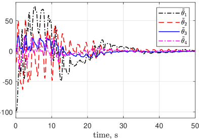
Figure 2: $\tilde{\theta}(t)$ with gradient algorithm (14ax) and $u_{pa}(t)$

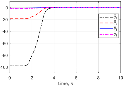
Figure 3: $\tilde{\theta}(t)$ with DREM procedure, estimator (14ay) and $u_{pa}(t)$

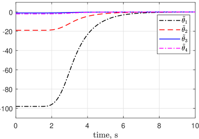
Figure 4: $\tilde{\theta}(t)$ with DREM procedure and new LRE, estimator (14az) and $u_{pa}(t)$

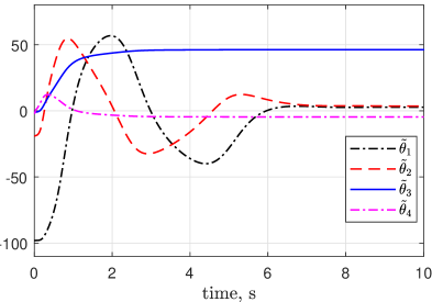
Figure 5: $\tilde{\theta}(t)$ with gradient algorithm (14ax) and $u_{pb}(t)$

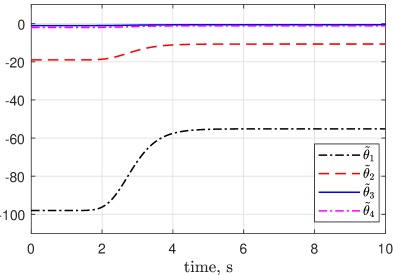
Figure 6: $\tilde{\theta}(t)$ with DREM procedure, estimator (14ay) and $u_{pb}(t)$

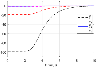
Figure 7: $\tilde{\theta}(t)$ with DREM procedure and new LRE, estimator (14az) and $u_{pb}(t)$

To test the robustness of the various estimators bounded noise was added to the output signal, as shown in Fig. 8), for the case of the input $u_{pb}(t)$.

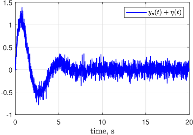
Figure 8: $y_{p}(t)$ with additive noise $\eta(t)$

As expected, in this case none of the estimators ensures that the error $\tilde{\theta}(t)$ converges to zero, as shown in Figs. 9-11. However, notice that the gradient algorithm (14ax) actually diverges. On the other hand, while the steady state error of the estimator with DREM (14ay) is quite large, the one of (14az) with the new LRE, is negligible—illustrating the robustness to additive noise of the the new scheme.

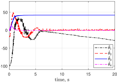
Figure 9: $\tilde{\theta}(t)$ (under the influence of $\eta(t)$) with gradient algorithm (14ax) and $u_{pb}(t)$

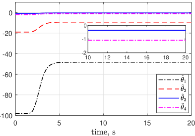
Figure 10: $\tilde{\theta}(t)$ (under the influence of $\eta(t)$) with DREM procedure, estimator (14ay) and $u_{pb}(t)$

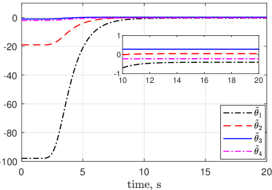
Figure 11: $\tilde{\theta}(t)$ (under the influence of $\eta(t)$) with DREM procedure and new filter, estimator (14az) and $u_{pb}(t)$

6 Simulations of the Discrete-time LRE Generator

In this section, we present comparative simulations of the DT estimation of a scalar parameter $\theta\in\mathbb{R}$ using the standard gradient descent adaptation with the original and the new regressor, that is,

$$\hat{\theta}_{\bf ori}(k+1)= \hat{\theta}_{\bf ori}(k)+\gamma\Delta(k)\left[\mathcal{Y}(k)-\Delta(k)\hat{\theta}_{\bf ori}(k)\right],\;\gamma>0$$ (14bc)

$$\hat{\theta}_{\bf new}(k+1)= \hat{\theta}_{\bf new}(k)+\gamma\Phi_{2}(k)\left[Y_{2}(k)-\Phi_{2}(k)\hat{\theta}_{\bf new}(k)\right],\;\gamma>0,$$ (14bd)

for three different signals $\Delta(k)$, namely:

$$\begin{aligned} \Delta_{a}(k)&=e^{-3k}\\ \Delta_{b}(k)&=\left\{\begin{aligned} 1&&k\in[0,0.2]\\ 0&&k>\mbox{0.2}\end{aligned}\right.\\ \Delta_{c}(k)&={1\over 7+k}.\end{aligned}$$ (14be)

Clearly, the three signals are not PE and belong to ${\mathcal{L}}_{2}$. Hence, according with Proposition LABEL:pro3 the estimator (14bc) will not converge. On the other hand, since they are IE, the estimator (14bd) should guarantee convergence for small values of $T$.

In the first simulations we consider the unknown parameter $\theta=5$ and select $\beta=\frac{3}{4}$, $\mu=0.4$, $b=0.1$ and $\gamma=0.1$. The initial conditions of the estimators are set as $\hat{\theta}_{{\bf ori}}(0)=0$ and $\hat{\theta}_{{\bf new}}(0)=0$. In the light of the key assumption (LABEL:tsqu) we also check the effect of the size of the constant $T$, carrying out simulations using the values $T=0.01$, $T=0.1$ and $T=1.5$.

The results of these simulations are given in Figs. 12-14, that confirm the predictions of the theoretical analysis. We also notice that taking a large value for $T$ does not affect the steady-state performance, but it increases significantly the convergence time. The rationale for this behavior may be explained as follows. In the scenarios considered above the signals $\Delta(k)$ converge to zero, reducing the effect of the truncation error.

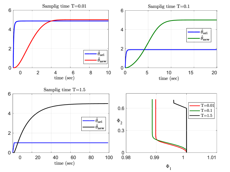
Figure 12: Estimates using the original and new LRE and the phase portrait of $\Phi(k)$ with the signal $\Delta_{a}(k)$

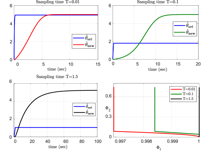
Figure 13: Estimates using the original and new LRE and the phase portrait of $\Phi(k)$ with the signal $\Delta_{b}(k)$

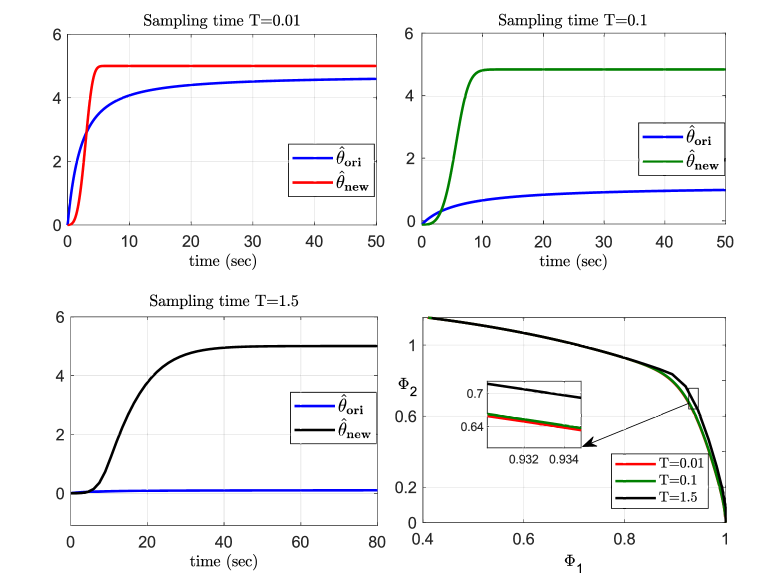
Figure 14: Estimates using the original and new LRE and the phase portrait of $\Phi(k)$ with the signal $\Delta_{c}(k)$

The situation is different if $\Delta(k)$ does not converge to zero, for instance if it is PE. In that case, it is expected that the performance is degraded with increasing values of $T$. To validate this conjecture we carried out a simulation with the PE signal $\Delta_{d}(k)=\cos\left(\frac{\pi}{4}k\right)$. In this case the estimator (14bc) always converges. However, (14bd) will ensure parameter convergence only for small values of $T$. This is corroborated with the plots of Fig. 15 that show how the performance of the estimator (14bd) degrades with increasing $T$. Moreover, from the phase portrait we notice that for $T=1.5$ the signal $\Phi(k)$ does not live in the gray section indicated in Fig. LABEL:fig1, violating the predictions of the theory because assumption (LABEL:tsqu) is not valid anymore. Furthermore, using the same $\Delta_{d}(k)$ and $T=1.5$, and choosing a large adaptation gain $\gamma=1.6$—in contrast to $\gamma=0.1$ used before – the estimator (14bd) becomes unstable as shown in Fig. 16. It is important to underscore that the main motivation for the introduction of the LRE generator is for the case when the original regressor is not PE, therefore the scenario considered in these simulations will not be encountered in practice.

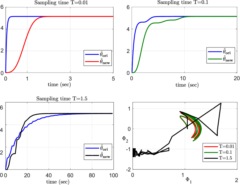
Figure 15: Estimates using the original and new LRE and the phase portrait of $\Phi(k)$ with the signal $\Delta_{d}(k)$

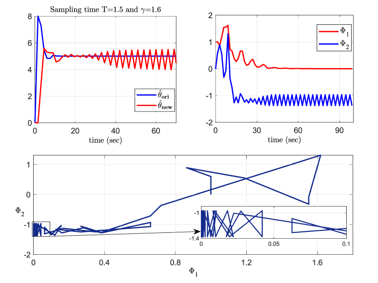
Figure 16: Estimates using the original and new LRE and the phase portrait of $\Phi(k)$ with the signal $\Delta_{d}(k)$ and $\gamma=1.6$

7 Conclusions and Future Research

We have proposed new CT and DT estimators for the LRE (1) that ensure global exponential convergence under the weak assumption that the regressor $\Omega$ is IE. To the best of our knowledge, this is the first time that such a result is established for a truly on-line estimator.

Our current efforts are directed towards the relaxation of the assumption (LABEL:tsqu) for the DT estimator and to further study the effect of noise in the estimators performance.

Appendix A List of Acronyms

CT	Continuous-time
DREM	Dynamic regressor extension and mixing
DT	Discrete-time
IE	Interval excitation
KRE	Kreisselmeier’s regressor extension
LRE	Linear regressor equation
LTI	Linear time-invariant
PE	Persistent excitation

References

- [1] S. Aranovskiy, A. Belov, R. Ortega, N. Barabanov and A, Bobtsov, Parameter identification of linear time‐invariant systems using dynamic regressor extension and mixing. International Journal of Adaptive Control and Signal Processing, vol. 33, no. 6, pp. 1016-1030, 2019.
- [2] S. Aranovskiy, A. Bobtsov, R. Ortega and A. Pyrkin, Performance enhancement of parameter estimators via dynamic regressor extension and mixing, IEEE Trans. on Automatic Control, vol. 62, pp. 3546-3550, 2017. (See also arXiv:1509.02763 for an extended version.)
- [3] S. Aranovskiy, R. Ushirobira, M. Korotina and A. Vedyakov, On preserving-excitation properties of a dynamic regressor extension scheme, IEEE Trans. on Automatic Control, (submitted, see also https://hal-centralesupelec.archives-ouvertes.fr/hal-03245139/document), 2021.
- [4] A. Belov, R. Ortega and A. Bobtsov, Guaranteed performance adaptive identification scheme of discrete-time systems using dynamic regressor extension and mixing, 18th IFAC Symposium on System Identification, (SYSID 2018), Stockholm, Sweden, July 9-11, 2018.
- [5] A. Bobtsov, B. Yi, R. Ortega and A. Astolfi, Generation of new exciting regressors for consistent on-line estimation of a scalar parameter, IEEE Trans. on Automatic Control, (submitted), 2021. (arXiv preprint: arXiv:2104.02210.)
- [6] G. Chowdhary, T. Yucelen, M. Muhlegg and E. N. Johnson, Concurrent learning adaptive control of linear systems with exponentially convergent bounds, International Journal of Adaptive Control and Signal Processing, vol. 27, no. 4, pp. 280–301, 2013.
- [7] D. Gerasimov, R. Ortega and V. Nikiforov, Adaptive control of multivariable systems with reduced knowledge of high frequency gain: Application of dynamic regressor extension and mixing estimators, 18th IFAC Symposium on System Identification, (SYSID 2018), Stockholm, Sweden, July 9-11, 2018.
- [8] G.C. Goodwin and K.S. Sin, Adaptive Filtering Prediction and Control, Prentice-Hall, 1984.
- [9] G. Kreisselmeier, Adaptive observers with exponential rate of convergence, IEEE Trans. on Automatic Control, vol. 22, no. 1, pp. 2-8, 1977.
- [10] G. Kreisselmeier and G. Rietze-Augst, Richness and excitation on an interval—with application to continuous-time adaptive control, IEEE Trans. on Automatic Control, vol. 35, no. 2, pp. 165-171, 1990.
- [11] G. Tao, Adaptive control design and analysis. Vol. 37. John Wiley & Sons, New Jersey, 2003.
- [12] F. Lewis, D. Vrabie, and K. Vamvoudakis, Reinforcement learning and feedback control: Using natural decision methods to design optimal adaptive controllers, IEEE Control Systems Magazine, vol. 32, no. 6, pp. 76–105, 2012.
- [13] L. Ljung, System Identification: Theory for the User, Prentice Hall, New Jersey, 1987.
- [14] R. Ortega, An on-line least-squares parameter estimator with finite convergence time, Proc. IEEE, vol. 76, no. 7, 1988.
- [15] R. Ortega, A. Bobtsov, A. Pyrkin and A. Aranovskiy, A parameter estimation approach to state observation of nonlinear systems, Systems and Control Letters, vol. 85, pp 84-94, 2015.
- [16] R. Ortega, A. Bobtsov, N. Nikolaev, J. Schiffer, D. Dochain, Generalized parameter estimation-based observers: Application to power systems and chemical-biological reactors, Automatica, vol. 129, 109635, 2021.
- [17] R. Ortega, V. Nikiforov and D. Gerasimov, On modified parameter estimators for identification and adaptive control: a unified framework and some new schemes, Annual Reviews in Control, vol. 50, pp. 278-293, 2020.
- [18] R. Ortega, S. Aranovskiy, A. Pyrkin, A Astolfi and A. Bobtsov, New results on parameter estimation via dynamic regressor extension and mixing: Continuous and discrete-time cases, IEEE Trans. on Automatic Control, (10.1109/TAC.2020.3003651), 2020.
- [19] R. Ortega, V. Gromov, E. Nuño, A. Pyrkin and J. G. Romero, Parameter estimation of nonlinearly parameterized regressions: application to system identification and adaptive control, Automatica, vol.. 127, 109544, May 2021.
- [20] R. Ortega, A definition of robustness with respect to initial conditions for nonlinear time-varying systems, Asian J. of Control, (DOI: 10.1002/asjc.2021).
- [21] Y. Pan and H. Yu, Composite learning robot control with guaranteed parameter convergence, Automatica, vol. 89, pp. 398–406, 2018.
- [22] S. Sastry and M. Bodson, Adaptive Control: Stability, Convergence and Robustness, Prentice-Hall, New Jersey, 1989.
- [23] J. Stoer and R. Bulirsch, Introduction to Numerical Analysis, Springer-Verlag, NY, 1983.
- [24] B. Yi, R. Ortega, D. Wu and W. Zhang, Orbital stabilization of nonlinear systems via Mexican sombrero energy pumping-and-damping injection. Automatica, vol. 112, 108-861, 2020.