Deep neural networks for high harmonic spectroscopy in solids

Abstract

Neural networks are a prominent tool for identifying and modeling complex patterns, which are otherwise hard to detect and analyze. While machine learning and neural networks have been finding applications across many areas of science and technology, their use in decoding ultrafast dynamics of quantum systems driven by strong laser fields has been limited so far. Here we use deep neural networks to analyze simulated noisy spectra of highly nonlinear optical response of a 2-dimensional gapped graphene crystal to intense few-cycle laser pulses. We show that a computationally simple 1-dimensional system provides a useful ”nursery school” for our neural network, allowing it to be easily retrained to treat more complex systems, recovering the band structure and spectral phases of the incident few-cycle pulse with high accuracy, in spite of significant amplitude noise and phase jitter. Our results both offer a new tool for attosecond spectroscopy of quantum dynamics in solids and also open a route to developing all-solid-state devices for complete characterization of few-cycle pulses, including their nonlinear chirp and the carrier envelope phase.

Electrons provide the fundamental first step in response of matter to light. The feasibility of shaping light pulses at the scale of individual oscillations, from mid-IR to UV Wirth et al. (2011); Hassan et al. (2016), offers rich opportunities for controlling electronic response to light on sub-cycle timescale (e.g. Schultze et al. (2013); Schiffrin et al. (2013); Kelardeh et al. (2016, 2015); Motlagh et al. (2019); Garg et al. (2016); Lakhotia et al. (2020); Vampa et al. (2015a); Reimann et al. (2018); Langer et al. (2018); Jimenez-Galan et al. (2019)), leading to a variety of fascinating phenomena such as optically induced anomalous Hall effect Motlagh et al. (2020); Sato et al. (2019); McIver et al. (2020), topological phase transitions with polarization-tailored light Jimenez-Galan et al. (2019), or the topological resonance Motlagh et al. (2019). Over multiple laser cycles, control of electron dynamics with light also enables the so-called Floquet engineering – the tailored modification of the cycle-average properties of a light-dressed system, see e.g. Oka and Kitamura (2019) for a recent review.

In this context, starting with the pioneering work Ghimire et al. (2011), high harmonic spectroscopy has developed into a powerful tool for exploring laser-driven electron dynamics in solids, see e.g. recent reviews  Vampa and Brabec (2017); Kruchinin et al. (2018); Ghimire and Reis (2019). Examples include identification of the common physical mechanisms underlying high harmonic generation in atoms, molecules and solids (e.g. Vampa et al. (2015a, b)), observation of Bloch oscillations Schubert et al. (2014), resolving interfering pathways of electrons in crystals with about 1-fsec precision Hohenleutner et al. (2015), inducing Jimenez-Galan et al. (2019) and monitoring topological Silva et al. (2019); Chacón et al. (2020); Bauer and Hansen (2018) and Mott insulator-to-metal Silva et al. (2018) phase transitions, resolving coherent oscillation of electronic charge density order Nag et al. (2019), identifying the van Hove singularities in the conduction bands Uzan et al. (2020), and reconstructing effective potentials seen by the light-driven electrons with picometer accuracy Lakhotia et al. (2020).

Here we apply machine learning to the analysis of high harmonic generation from a crystal, which allows us to ’kill two birds with one stone’: reconstruct the band structure of the crystal and fully characterize incident few-cycle laser pulses, including both their nonlinear chirp and the phase of the carrier oscillations under the envelope (CEP).

The fundamental role of the CEP in nonlinear light-matter interaction has been understood theoretically in de Bohan et al. (1998); Cormier and Lambropoulos (1998); Tempea et al. (1999); Dietrich et al. (2000), stimulating first experiments in the gas phase Paulus et al. (2001). Powerful gas-phase methods for characterizing few-cycle pulses have been developed, including stereo-above-threshold ionization (stereo-ATI) Zhang et al. (2017); Paulus et al. (2003); Milošević et al. (2006), attosecond streak camera and its modifications Goulielmakis et al. (2004); Itatani et al. (2002); Mairesse and Quéré (2005); Baltuška et al. (2003); Kienberger et al. (2004), and half-cycle high harmonic cutoffs Haworth et al. (2007). Using nonlinear response of solids for characterizing the CEP has also been pursued Dombi et al. (2004); Apolonski et al. (2004); Paasch-Colberg et al. (2013). Yet, all-optical, all-solid-state characterization of few-cycle pulses, including their CEP, remains a challenge. We hope to change this situation. Particularly relevant to our work are the earlier proposal on using interference patterns in spectrally overlapping regions of even- and odd-order harmonics in solids Mehendale et al. (2000) and the use of two-color high harmonic spectroscopy for all-optical reconstruction of the band structure Vampa et al. (2015c) from the two-dimensional high harmonic spectra, recorded as a function of the harmonic frequency and the two-color delay.

Two-dimensional spectra of the nonlinear-optical response may provide sufficient information to recover the pulse. One prominent example is frequency-resolved optical gating, which uses the second-order optical response recorded as a function of the time-delay between the two incident pulses, the target pulses and the auxiliary gate pulse (e.g. Trebino and Kane (1993); Miranda et al. (2012); Mairesse and Quéré (2005).) Extending this analysis to highly nonlinear optical response remains an open problem. The crucial importance of addressing this problem stems from the fact that such analysis would allow one to characterize the laser pulse directly in the interaction region.

In special cases, such as the case of the two-color high harmonic spectroscopy of attosecond pulses using fundamental and the second harmonic (e.g. Dudovich et al. (2006)), the 2D harmonic spectra recorded as a function of the two-color phase and the harmonic frequency may carry sufficient information for reconstructing attosecond pulses as they are produced, directly in the interaction region. Such reconstruction does, however, require detailed understanding of the physics of the microscopic quantum response. The possibility of solving a full reconstruction problem in a general case, recovering both the pulse and the quantum system, remains completely unexplored.

When there is no simple and/or well known functional dependence between the response data and the parameters one wishes to reconstruct, the problem is well suited for neural networks. Such networks aim to find a smooth analytical function $f_{\theta}(x)$ which connects the input $x_{i}$ and the desired output $y_{i}$. If it is successful, one can conclude that the data $x$ indeed does contain the information $y$. Pertinent examples include applications to solving the Schrödinger equation, where neural networks can output highly accurate results Mills et al. (2017); Giri et al. (2021). Our results show that, given sufficient training set, the 2D spectra of the high harmonic response as a function of the nonlinear response frequency and the CEP of an unknown driving pulse allow for simultaneous reconstruction of both the pulse and the unknown crystal band structure, even in the presence of substantial noise including CEP jitter.

To demonstrate the method, we assume no apriori knowledge about the incident pulse and use rather limited knowledge about the nonlinear medium. For the quantum system, we begin with a modified Rice-Mele model Rice and Mele (1982) with nearest neighbor, next nearest neighbor, etc. hoppings, see Figure 1(a) (and Supplementary information for further details.) Both the on-site energies and the couplings are assumed to be unknown. The reconstruction procedure is expected to output both the parameters of the pulse and of the lattice. We are thus faced with a nonlinear optimization problem with a very large input dimension, which requires finding optimal interpolation between the existing trial samples.

Such a regression tool is provided by deep neural networks (DNNs) Carleo et al. (2019), already used for such diverse applications as boosting the signal-to-noise ratio in LHC collision data Baldi et al. (2014), establishing a fast mapping between galaxy and dark matter distribution Zhang et al. (2019), and constructing efficient representations of many-body quantum states Sharir et al. (2020). The inherent resilience of neural networks to noise is an important asset for pulse shape characterization. The emergence of photonic implementations of feed-forward neural networks Shen et al. (2017) outlines a perspective of implementing this regression scheme in an all-optical way.

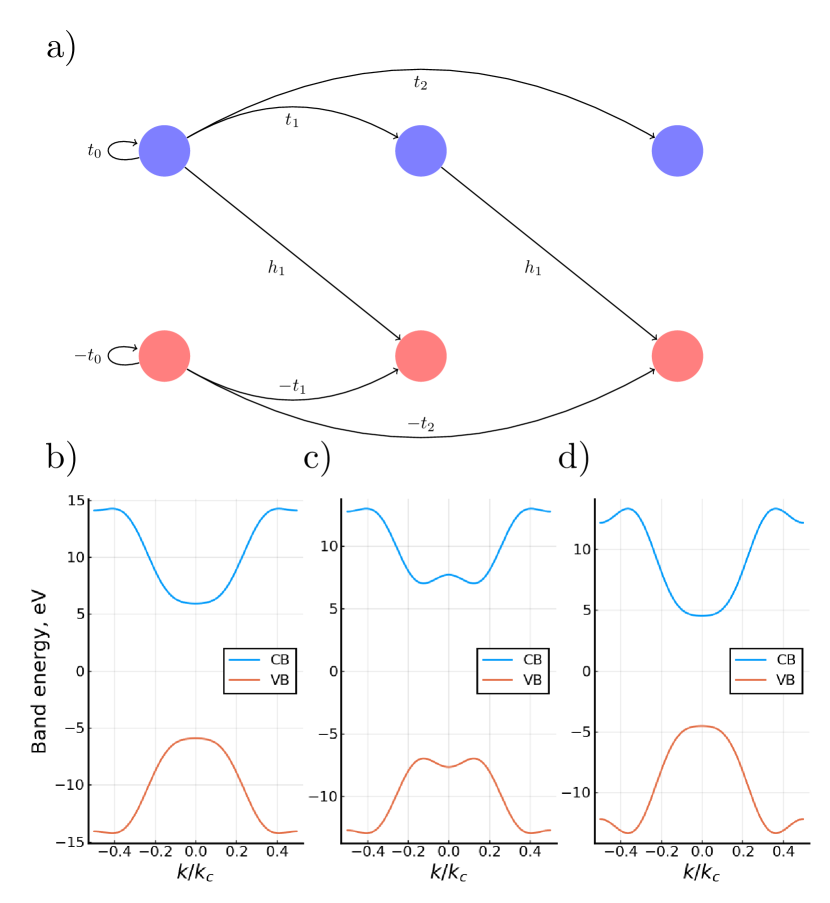
Figure 1: Model system used for pulse reconstruction and band structure spectroscopy via nonlinear-optical response. (a) The two types of sites present, A and B, are connected by hopping constants $t_{j}$ between similar sites and $h_{1}$ between the next-neighbor sites of the different type. (b-d) Examples of band structures that can be generated with this model system.

The vector potential of the incident laser field, $A(t)$, is generated in the frequency domain with the unknown to the neural network quadratic and the cubic phases:

$$A(\omega)\propto\exp(i\phi(\omega))=\exp\left(i\lambda(\omega-\omega_{0})^{3}/6-\mu(\omega-\omega_{0})^{2}/2+i\varphi\right)$$ (1)

The complex parameter $\mu$ is defined in such a way that, in the absence of the cubic chirp, the pulse has a temporal width $\sigma\equiv T_{0}$: $\mu\equiv\cfrac{\sigma^{2}-i\alpha}{1+\alpha^{2}/\sigma^{4}}$, where $\alpha$ is the chirp parameter. The chirp parameters $\alpha$ and $\lambda$ are expressed via dimensionless quantities $\beta$ and $\epsilon$, $\alpha=\pi(\sigma/2)^{2}\times\beta$, $\lambda=\pi\sigma^{3}\times\epsilon$. The dimensionless parameters vary in the ranges $\beta\in\left[-2.0,2.0\right],\epsilon\in\left[-1.0,1.0\right]$. Finally, $\varphi$ sets the CEP of the pulse, also unknown to the neural network and chosen randomly. The system evolution is simulated for 40 laser cycles; an additional Gaussian cutoff is introduced at the leading and trailing edges of the pulse for numerical stability (see Supplementary information.)

The typical pulses we have used for reconstruction are shown in Fig. 2, both in time and frequency domain. The latter shows the spectral phases (red curves) alongside the spectral amplitudes (blue curves), as a function of $\omega/\omega_{0}$, where $\omega_{0}$ is the carrier. Our typical simulated ”measurement” assumes that one can systematically vary the (unknown) CEP. Thus, we perform calculations by varying $\varphi+\Delta\varphi$, with $\Delta\varphi$ spanning the full range $\Delta\varphi\in\left[0,2\pi\right)$. For each $\Delta\varphi$, we measure the absolute value of the spectral amplitude of the laser-induced current $|j(\omega)|$, which is given by the Fourier transform of the calculated current $j(t)$.

Figure 2: Sample pulse shapes used in the problem. (a-c) show the time-domain. (d-f) are the frequency-domain representations of their respective pulses, where the spectral phase (red line) and spectral amplitude normalized to the central frequency amplitude (blue area), are plotted with respect to frequency. The pulse parameters are $(\varphi,\beta,\epsilon)$, left to right: $(\pi/2,0.0,0.0),(0.0,2.0,0.0),(0.0,1.0,1.0)$.

The input data is composed of the absolute values of the integer harmonic amplitudes $|j(N\omega,\varphi+\Delta\varphi)|$. The resulting 2D map as a function of $\Delta\varphi$ and $\omega$ is used as the input into the neural network. The network must then infer the (randomly chosen in each trial) intraband hoppings $\{t_{j}\}$, the unknown initial CEP $\varphi$, and the pulse parameters $\alpha$ and $\lambda$. The values of $\sigma$, frequency $\omega$, and $h_{1}$ are kept constant throughout. For more information about the inputs used, see Supplementary information.

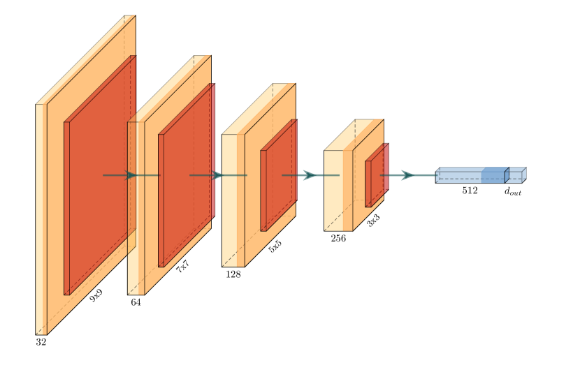
Figure 3: Network architecture used in the paper. Yellow denotes a convolution layer with the number of filters below, orange a batch normalization with subsequent Swish activation, red a maximum pooling layer, blue a fully connected layer, dark blue a Swish activation with no preceding batch normalization. The output of the last FC layer is linear.

In the reconstruction procedure, we have used two separate neural networks, one for recovering the band parameters, and another for recovering the CEP and pulse parameters. Both are constructed using the same architecture, consisting of 4 convolutional layers and two fully-connected ones, see Fig. 3. Constructing them as a single neural network with split fully connected layer impedes the overall performance of the scheme. For either problem, this network is trained for 200 epochs with the AdaBelief Zhuang et al. (2020) optimizer with batch size 256; the learning rate is initially set to $10^{-3}$ and discounted at the 150th epoch by a factor of 10.

To speed up training, we train networks to work on more complex datasets (e.g. with chirped pulses) by using a network pre-trained on a simpler dataset (e.g. with no chirp). The rest of the training procedure remains the same, but the overall number of epochs is reduced to 50.

The recovery results are demonstrated in Fig. 4. The number of unknown band parameters is set to 4. The agreement between the actual and the reconstructed data, both for the system and for the pulse, is excellent. Tables with detailed analysis of the average performance are given in the supplementary material.

Figure 4: Band parameters (a-d) and CEP (e, f) recovered by the neural network for the source problem (Rice-Mele model, no chirp or cubic phase). The solid orange line $y=x$ serves as a reference. All points used belong to the test set.

We now also demonstrate that our neural network recovers the system parameters with comparable precision when the input-data contains experiment-like noise. We use a network pretrained on the initial noiseless dataset with no chirp or cubic phase. To simulate experimental noise, we have introduced a random CEP shift to each of the pulses in each sample, sampled from a uniform distribution within $-50\div 50\text{ mrad}$. The output amplitudes were also affected by a uniformly-distributed multiplicative noise with an amplitude of 0.1. The exact performance figures with and without added noise can be found in the supplementary information.

After demonstrating that our neural network recovers the band structure and pulse parameters of the simple source (Rice-Mele) model with high accuracy, we apply our approach to more complex systems. As an example of such more complex system, we used the 2-dimensional gapped graphene system. Its parameters (on-site energy and first-neighbor hopping) were generated in the vicinity of experimental values for hBN, within $4.0\div 7.27$ eV and $0.08\div 0.16$ a.u., respectively. We simulated its responses by integrating the semiconductor Bloch equations. To simulate experimental conditions, we applied noise using the same procedure as described above.

Due to the greater computational cost, we could only use 1280 samples as opposed to 65536 for the source problem. Such a dataset is too small to train an entire new network. Instead, we applied the transfer learning approach by using the networks pre-trained on datasets with no quadratic or cubic phase, varying the CEP, and 4 unknown band parameters, and partially retraining them (see Supplementary). We discovered that, in spite of the greater complexity of the underlying physical system, such a setup recovers the CEP with a precision comparable to the original problem (see Figs. 5), and achieves good relative accuracy on the band parameters.

This adds new significance to the achieved results. Indeed, we have now demonstrated that the spectra from the initial model, while only resembling a real-world setup in a qualitative sense, provide a useful training ground for the neural network, allowing it to acquire useful abstract concepts (parameterized by the deeper layers) which it can later apply to more practical problems, for which it was also harder to generate as many training samples.

Figure 5: Band structure (a), pulse waveform (b), and CEP (c, d) recovered by the neural network for the target problem (2-dimensional gapped graphene with phase and multiplicative noise).

Our results demonstrate that solid-state HHG spectra contain more information than one extracts with conventional methods: not only the pulse parameters, but also the parameters of the quantum system are robustly reconstructed. Our approach replicates the advantages of gas-phase HHG spectroscopy, namely, the ability to resolve the CEP of laser pulses and the complex pulse shapes with polynomial spectral phase nonlinearities. At the same time, it requires neither the XUV pulses nor the photoelectron spectroscopy, such as the stereo-ATI. Moreover, it allows for all-optical solid-state implementation. In terms of required observables, it is closest to the method based on measuring the half-cycle cutoffs in gas-phase high harmonic generation Haworth et al. (2007). However, it also allows one to deal with very strong chirps. Applying neural networks to the analysis of half-cycle cutoffs and high harmonic generation spectra in the gas phase could be very interesting, especially in molecules, where multiple coupled harmonic generation channels present challenges for unravelling the underlying laser-driven multi-electron dynamics Bruner et al. (2016).

One could apply the developed neural network design to standard gas-phase experiments, to analyse the possibility of resolving the spectral phase and the CEP for short pulses by processing HHG spectra generated by known inert gases (Ar, Ne, etc.). In this case the neural network can be trained using TDSE simulations of the necessary responses before being applied to real experimental data.

The key difficulty of using high harmonic spectroscopy in solids is that, without apriori knowledge of the band structure, one lacks closed-form solutions for electron dynamics, similar to those available in the gas-phase. Our method circumvents this difficulty. Pulse characterization device implementing our principles could be tabletop, all solid-state, and capable of operating at ambient conditions.

Another interesting direction to pursue would be to apply novel physics-informed neural network architecturesGreydanus et al. (2019); Toth et al. (2019) to resolve Hamiltonians of systems with many degrees of freedom (such as molecules) using time-resolved HHG spectra, such as those obtained from solids driven by mid-IR fields Hohenleutner et al. (2015). Neural networks can also be used for processing the sets of harmonic spectra connected by other relations, such as being measured for different angles between the crystal axes and the driving field, to uncover effective laser-modified potentials for the charge motion, extending the pioneering work in Ref. Lakhotia et al. (2020) to recover effective potentials of active band electrons. Here, once again, one can take advantage of our idea of using neural networks to extend a method of processing analytically-tractable systems to intractable ones, recovering effective structures.

I Funding

M.I. and N.K. acknowledge funding of the DFG QUTIF grant IV152/6-2. N.K. acknowledges funding by the Foundation for Assistance to Small Innovative Enterprises (agreement No 196GUTsES8-D3/56338) and Foundation for the Advancement of Theoretical Physics and Mathematics (agreement No 20-2-2-39-1). This project has received funding from the European Union’s Horizon 2020 research and innovation programme under grant agreement No 899794.

II Acknowledgements

We thank Vera V. Tiunova for her useful feedback. N.K. and M.I. developed the idea behind the paper and wrote the manuscript. N.K., Á. J.-G. and R.E.F.S. performed the calculations. N.K. designed the neural network architecture.

III Disclosures

The authors declare no competing interests.

IV Data availability

The generated datasets, trained neural network weights, and reconstructed values are available in Dataset 1 (Ref. Klimkin et al. ). The codes running the TDSE simulation and neural network reconstruction of parameters were written in the Julia language Bezanson et al. (2017) and are available publicly on GitHub Klimkin .

References

- Wirth et al. (2011) A. Wirth, M. T. Hassan, I. Grguraš, J. Gagnon, A. Moulet, T. T. Luu, S. Pabst, R. Santra, Z. A. Alahmed, A. M. Azzeer, V. S. Yakovlev, V. Pervak, F. Krausz, and E. Goulielmakis, Science 334, 195 (2011), https://science.sciencemag.org/content/334/6053/195.full.pdf .
- Hassan et al. (2016) M. T. Hassan, T. T. Luu, A. Moulet, O. Raskazovskaya, P. Zhokhov, M. Garg, N. Karpowicz, A. M. Zheltikov, V. Pervak, F. Krausz, and E. Goulielmakis, Nature 530, 66 (2016).
- Schultze et al. (2013) M. Schultze, E. M. Bothschafter, A. Sommer, S. Holzner, W. Schweinberger, M. Fiess, M. Hofstetter, R. Kienberger, V. Apalkov, V. S. Yakovlev, et al., Nature 493, 75 (2013).
- Schiffrin et al. (2013) A. Schiffrin, T. Paasch-Colberg, N. Karpowicz, V. Apalkov, D. Gerster, S. Mühlbrandt, M. Korbman, J. Reichert, M. Schultze, S. Holzner, et al., Nature 493, 70 (2013).
- Kelardeh et al. (2016) H. K. Kelardeh, V. Apalkov, and M. I. Stockman, Physical Review B 93, 155434 (2016).
- Kelardeh et al. (2015) H. K. Kelardeh, V. Apalkov, and M. I. Stockman, Physical Review B 91, 045439 (2015).
- Motlagh et al. (2019) S. A. O. Motlagh, F. Nematollahi, V. Apalkov, and M. I. Stockman, Physical Review B 100, 115431 (2019).
- Garg et al. (2016) M. Garg, M. Zhan, T. T. Luu, H. Lakhotia, T. Klostermann, A. Guggenmos, and E. Goulielmakis, Nature 538, 359 (2016).
- Lakhotia et al. (2020) H. Lakhotia, H. Kim, M. Zhan, S. Hu, S. Meng, and E. Goulielmakis, Nature 583, 55 (2020).
- Vampa et al. (2015a) G. Vampa, T. Hammond, N. Thiré, B. Schmidt, F. Légaré, C. McDonald, T. Brabec, and P. Corkum, Nature 522, 462 (2015a).
- Reimann et al. (2018) J. Reimann, S. Schlauderer, C. Schmid, F. Langer, S. Baierl, K. Kokh, O. Tereshchenko, A. Kimura, C. Lange, J. Güdde, et al., Nature 562, 396 (2018).
- Langer et al. (2018) F. Langer, C. P. Schmid, S. Schlauderer, M. Gmitra, J. Fabian, P. Nagler, C. Schüller, T. Korn, P. Hawkins, J. Steiner, et al., Nature 557, 76 (2018).
- Jimenez-Galan et al. (2019) A. Jimenez-Galan, R. E. F. Silva, O. Smirnova, and M. Ivanov, “Lightwave topology for strong-field valleytronics,” (2019), arXiv:1910.07398 [physics.optics] .
- Motlagh et al. (2020) S. A. O. Motlagh, V. Apalkov, and M. I. Stockman, “Anomalous ultrafast all-optical hall effect in gapped graphene,” (2020), arXiv:2007.12757 [cond-mat.mes-hall] .
- Sato et al. (2019) S. Sato, P. Tang, M. Sentef, U. De Giovannini, H. Hübener, and A. Rubio, New Journal of Physics 21, 093005 (2019).
- McIver et al. (2020) J. W. McIver, B. Schulte, F.-U. Stein, T. Matsuyama, G. Jotzu, G. Meier, and A. Cavalleri, Nature physics 16, 38 (2020).
- Oka and Kitamura (2019) T. Oka and S. Kitamura, Annual Review of Condensed Matter Physics 10, 387 (2019).
- Ghimire et al. (2011) S. Ghimire, A. D. DiChiara, E. Sistrunk, P. Agostini, L. F. DiMauro, and D. A. Reis, Nature physics 7, 138 (2011).
- Vampa and Brabec (2017) G. Vampa and T. Brabec, Journal of Physics B: Atomic, Molecular and Optical Physics 50, 083001 (2017).
- Kruchinin et al. (2018) S. Y. Kruchinin, F. Krausz, and V. S. Yakovlev, Reviews of Modern Physics 90, 021002 (2018).
- Ghimire and Reis (2019) S. Ghimire and D. A. Reis, Nature Physics 15, 10 (2019).
- Vampa et al. (2015b) G. Vampa, C. McDonald, G. Orlando, P. Corkum, and T. Brabec, Physical Review B 91, 064302 (2015b).
- Schubert et al. (2014) O. Schubert, M. Hohenleutner, F. Langer, B. Urbanek, C. Lange, U. Huttner, D. Golde, T. Meier, M. Kira, S. W. Koch, et al., Nature Photonics 8, 119 (2014).
- Hohenleutner et al. (2015) M. Hohenleutner, F. Langer, O. Schubert, M. Knorr, U. Huttner, S. W. Koch, M. Kira, and R. Huber, Nature 523, 572 (2015).
- Silva et al. (2019) R. Silva, Á. Jiménez-Galán, B. Amorim, O. Smirnova, and M. Ivanov, Nature Photonics 13, 849 (2019).
- Chacón et al. (2020) A. Chacón, D. Kim, W. Zhu, S. P. Kelly, A. Dauphin, E. Pisanty, A. S. Maxwell, A. Picón, M. F. Ciappina, D. E. Kim, et al., Physical Review B 102, 134115 (2020).
- Bauer and Hansen (2018) D. Bauer and K. K. Hansen, Physical Review Letters 120, 177401 (2018).
- Silva et al. (2018) R. Silva, I. V. Blinov, A. N. Rubtsov, O. Smirnova, and M. Ivanov, Nature Photonics 12, 266 (2018).
- Nag et al. (2019) T. Nag, R.-J. Slager, T. Higuchi, and T. Oka, Physical Review B 100, 134301 (2019).
- Uzan et al. (2020) A. J. Uzan, G. Orenstein, Á. Jiménez-Galán, C. McDonald, R. E. Silva, B. D. Bruner, N. D. Klimkin, V. Blanchet, T. Arusi-Parpar, M. Krüger, et al., Nature Photonics 14, 183 (2020).
- de Bohan et al. (1998) A. de Bohan, P. Antoine, D. B. Milošević, and B. Piraux, Physical review letters 81, 1837 (1998).
- Cormier and Lambropoulos (1998) E. Cormier and P. Lambropoulos, The European Physical Journal D-Atomic, Molecular, Optical and Plasma Physics 2, 15 (1998).
- Tempea et al. (1999) G. Tempea, M. Geissler, and T. Brabec, JOSA B 16, 669 (1999).
- Dietrich et al. (2000) P. Dietrich, F. Krausz, and P. Corkum, Optics letters 25, 16 (2000).
- Paulus et al. (2001) G. Paulus, F. Grasbon, H. Walther, P. Villoresi, M. Nisoli, S. Stagira, E. Priori, and S. De Silvestri, Nature 414, 182 (2001).
- Zhang et al. (2017) Y. Zhang, P. Kellner, D. Adolph, D. Zille, P. Wustelt, D. Würzler, S. Skruszewicz, M. Möller, A. M. Sayler, and G. G. Paulus, Opt. Lett. 42, 5150 (2017).
- Paulus et al. (2003) G. G. Paulus, F. Lindner, H. Walther, A. Baltuška, E. Goulielmakis, M. Lezius, and F. Krausz, Physical review letters 91, 253004 (2003).
- Milošević et al. (2006) D. Milošević, G. Paulus, D. Bauer, and W. Becker, Journal of Physics B: Atomic, Molecular and Optical Physics 39, R203 (2006).
- Goulielmakis et al. (2004) E. Goulielmakis, M. Uiberacker, R. Kienberger, A. Baltuska, V. Yakovlev, A. Scrinzi, T. Westerwalbesloh, U. Kleineberg, U. Heinzmann, M. Drescher, and F. Krausz, Science (New York, N.Y.) 305, 1267 (2004).
- Itatani et al. (2002) J. Itatani, F. Quéré, G. L. Yudin, M. Y. Ivanov, F. Krausz, and P. B. Corkum, Physical review letters 88, 173903 (2002).
- Mairesse and Quéré (2005) Y. Mairesse and F. Quéré, Physical Review A 71, 011401 (2005).
- Baltuška et al. (2003) A. Baltuška, T. Udem, M. Uiberacker, M. Hentschel, E. Goulielmakis, C. Gohle, R. Holzwarth, V. Yakovlev, A. Scrinzi, T. W. Hänsch, et al., Nature 421, 611 (2003).
- Kienberger et al. (2004) R. Kienberger, E. Goulielmakis, M. Uiberacker, A. Baltuska, V. Yakovlev, F. Bammer, A. Scrinzi, T. Westerwalbesloh, U. Kleineberg, U. Heinzmann, et al., Nature 427, 817 (2004).
- Haworth et al. (2007) C. Haworth, L. Chipperfield, J. Robinson, P. Knight, J. Marangos, and J. Tisch, Nature Physics 3 (2007), 10.1038/nphys463.
- Dombi et al. (2004) P. Dombi, A. Apolonski, C. Lemell, G. G. Paulus, M. Kakehata, R. Holzwarth, T. Udem, K. Torizuka, J. Burgdörfer, T. W. Hänsch, and F. Krausz, New Journal of Physics 6, 39 (2004).
- Apolonski et al. (2004) A. Apolonski, P. Dombi, G. G. Paulus, M. Kakehata, R. Holzwarth, T. Udem, C. Lemell, K. Torizuka, J. Burgdörfer, T. W. Hänsch, et al., Physical review letters 92, 073902 (2004).
- Paasch-Colberg et al. (2013) T. Paasch-Colberg, A. Schiffrin, N. Karpowicz, S. Kruchinin, Z. S. Lam, S. Keiber, O. Razskazovskaya, S. Muehlbrandt, A. Alnaser, M. Kübel, V. Apalkov, D. Gerster, J. Reichert, T. Wittmann, J. Barth, M. Stockman, R. Ernstorfer, V. Yakovlev, R. Kienberger, and F. Krausz, Nature Photonics 8 (2013), 10.1038/NPHOTON.2013.348.
- Mehendale et al. (2000) M. Mehendale, S. Mitchell, J.-P. Likforman, D. Villeneuve, and P. Corkum, Optics letters 25, 1672 (2000).
- Vampa et al. (2015c) G. Vampa, T. J. Hammond, N. Thiré, B. E. Schmidt, F. Légaré, C. R. McDonald, T. Brabec, D. D. Klug, and P. B. Corkum, Phys. Rev. Lett. 115, 193603 (2015c).
- Trebino and Kane (1993) R. Trebino and D. J. Kane, J. Opt. Soc. Am. A 10, 1101 (1993).
- Miranda et al. (2012) M. Miranda, C. L. Arnold, T. Fordell, F. Silva, B. Alonso, R. Weigand, A. L’Huillier, and H. Crespo, Opt. Express 20, 18732 (2012).
- Dudovich et al. (2006) N. Dudovich, O. Smirnova, J. Levesque, Y. Mairesse, M. Y. Ivanov, D. Villeneuve, and P. B. Corkum, Nature physics 2, 781 (2006).
- Mills et al. (2017) K. Mills, M. Spanner, and I. Tamblyn, Physical Review A 96, 042113 (2017).
- Giri et al. (2021) S. K. Giri, L. Alonso, U. Saalmann, and J. M. Rost, Faraday Discussions (2021).
- Rice and Mele (1982) M. Rice and E. Mele, Physical Review Letters 49, 1455 (1982).
- Carleo et al. (2019) G. Carleo, I. Cirac, K. Cranmer, L. Daudet, M. Schuld, N. Tishby, L. Vogt-Maranto, and L. Zdeborová, Rev. Mod. Phys. 91, 045002 (2019).
- Baldi et al. (2014) P. Baldi, P. Sadowski, and D. Whiteson, Nature Communications 5, 4308 (2014).
- Zhang et al. (2019) X. Zhang, Y. Wang, W. Zhang, Y. Sun, S. He, G. Contardo, F. Villaescusa-Navarro, and S. Ho, “From dark matter to galaxies with convolutional networks,” (2019), arXiv:1902.05965 [astro-ph.CO] .
- Sharir et al. (2020) O. Sharir, Y. Levine, N. Wies, G. Carleo, and A. Shashua, Physical Review Letters 124 (2020), 10.1103/physrevlett.124.020503.
- Shen et al. (2017) Y. Shen, N. C. Harris, S. Skirlo, M. Prabhu, T. Baehr-Jones, M. Hochberg, X. Sun, S. Zhao, H. Larochelle, D. Englund, and M. Soljačić, Nature Photonics 11, 441 (2017).
- Zhuang et al. (2020) J. Zhuang, T. Tang, Y. Ding, S. Tatikonda, N. Dvornek, X. Papademetris, and J. S. Duncan, arXiv preprint arXiv:2010.07468 (2020).
- Bruner et al. (2016) B. D. Bruner, Z. Mašín, M. Negro, F. Morales, D. Brambila, M. Devetta, D. Faccialà, A. G. Harvey, M. Ivanov, Y. Mairesse, et al., Faraday discussions 194, 369 (2016).
- Greydanus et al. (2019) S. Greydanus, M. Dzamba, and J. Yosinski, in Advances in Neural Information Processing Systems (2019) pp. 15379–15389.
- Toth et al. (2019) P. Toth, D. J. Rezende, A. Jaegle, S. Racanière, A. Botev, and I. Higgins, arXiv preprint arXiv:1909.13789 (2019).
- (65) N. Klimkin, A. Jiménez-Galán, and R. E.F. Silva, “Deep neural networks for high harmonic spectroscopy in solids: datasets,” https://cloud.rqc.ru/nextcloud/index.php/s/tmmBAm2BbgqgLoZ.
- Bezanson et al. (2017) J. Bezanson, A. Edelman, S. Karpinski, and V. B. Shah, SIAM review 59, 65 (2017).
- (67) N. Klimkin, “Deep neural networks for high harmonic spectroscopy in solids: supporting code,” https://github.com/KlimkinND/PulseReconstruction.