Central limit theorem for kernel estimator of invariant density in bifurcating Markov chains models.

Abstract.

Bifurcating Markov chains (BMC) are Markov chains indexed by a full binary tree representing the evolution of a trait along a population where each individual has two children. Motivated by the functional estimation of the density of the invariant probability measure which appears as the asymptotic distribution of the trait, we prove the consistence and the Gaussian fluctuations for a kernel estimator of this density based on late generations. In this setting, it is interesting to note that the distinction of the three regimes on the ergodic rate identified in a previous work (for fluctuations of average over large generations) disappears. This result is a first step to go beyond the threshold condition on the ergodic rate given in previous statistical papers on functional estimation.

Keywords: Bifurcating Markov chains, bifurcating auto-regressive process, binary trees, fluctuations for tree indexed Markov chain, density estimation.

Mathematics Subject Classification (2020): 62G05, 62F12, 60J05, 60F05, 60J80.

1. Introduction

Bifurcating Markov chains (BMC) are a class of stochastic processes indexed by regular binary tree and which satisfy the branching Markov property (see below for a precise definition). This model represents the evolution of a trait along a population where each individual has two children. The recent study of BMC models was motivated by the understanding of the cell division mechanism (where the trait of an individual is given by its growth rate). The first model of BMC, named “symmetric” bifurcating auto-regressive process (BAR), see Section 3.2 for more details in a Gaussian framework, were introduced by Cowan & Staudte [6] in order to analyze cell lineage data. In [11], Guyon has studied more general asymmetric BMC to prove statistical evidence of aging in Escherichia Coli. We refer to [2] for more detailed references on this subject. Recently, several statistical works have been devoted to the estimation of cell division rates, see Doumic, Hoffmann, Krell & Roberts [10], Bitseki, Hoffmann & Olivier [4] and Hoffmann & Marguet [13]. Moreover, another studies, such as Doumic, Escobedo & Tournus [9], can be generalized using the BMC theory (we refer to the conclusion therein).

In this paper, our objective is to study the functional estimation of the density of the invariant probability measure $\mu$ associated to the BMC. For this purpose, we develop a kernel estimation in the $L^{2}(\mu)$ framework under reasonable hypothesis (which are in particular satisfied by the Gaussian symmetric BAR model from Section 3.2). This approach is in the spirit of the $L^{2}(\mu)$ approach developed [1]. In BMC model, the evolution of the trait along the genealogy of an individual taken at random is Markovian. Let us assume it is geometrically ergodic with rate $\alpha\in(-1,1)$, with $\mu$ is its invariant measure. In [1], three regimes where identified for the rate of convergence of averages over large generations according to the ergodic rate of convergence $\alpha$ with respect to the threshold $1/\sqrt{2}$. It is interesting, and surprising as well, to note that the distinction of those three regimes disappears for the rate of convergence when considering the kernel density estimation of the density of $\mu$, see Theorem 3.6. However, let us mention that some further restriction on the admissible bandwidths of the kernel estimator are to be taken into account in the super-critical regime (i.e. $\alpha>1/\sqrt{2}$), to be precise see Condition (14) which is in force for Theorem 3.6. Furthermore, we get that estimations using different generations provide asymptotically independent fluctuations, see Remark 3.9 (see also the form of the asymptotic variance in Theorem 3.17 and Remark 3.18 in a more general framework); this phenomenon already appear in [7]. The convergence of the kernel estimator in Theorem 3.6 relies on different type of assumptions:

• Geometric ergodic rate $\alpha\in(0,1)$ of convergence for the evolution of the trait along the genealogy of an individual taken at random, see Assumption 2.4.

• Regularity (density and integrability conditions) for the evolution kernel ${\mathcal{P}}$ and the initial distribution of the BMC, see Assumptions 3.1, and 3.2. The former is in the spirit of [1] (see Assumption 3.11 which is a consequence of Assumption 3.1 as proven in Section 4.1).

• Regularity (isotropic Hölder regularity) of the density of $\mu$ with respect to the Lebesgue measure on $S={\mathbb{R}}^{d}$, see Assumption 3.4 (i).

• Regularity of the kernel function $K$ and on the bandwidth given in Assumption 3.3 and Assumption 3.4 (ii)-(iii).

• A condition on the bandwidth given in Equation (14) which add a further restriction only in the super-critical regime $\alpha>1/\sqrt{2}$.

Eventually, we present some simulations on the kernel estimation of the density of $\mu$. We note that in statistical studies which have been done in [10, 4, 5], the ergodic rate of convergence is assumed to be less than 1/2, which is strictly less than the threshold $1/\sqrt{2}$ for criticality. Moreover, in the latter works, the authors are interested in the non-asymptotic analysis of the estimators. Now, with the new perspective given by the present results, see in particular Remark 3.7, we think that the works in [10, 4, 5] can be extended to the case where the ergodic rate of convergence belongs to $(1/2,1)$.

The paper is organized as follows. We introduce the BMC model in Section 2 as well as the $L^{2}$ ergodic assumption. We define the kernel estimator and state the main results on the estimation of the density of $\mu$, see Lemma 3.5 (consistency) and Theorem 3.6 (asymptotic normality), in Section 3.1. The proofs of those result rely on a general central limit theorem, see Theorem 3.17 in Section 3.4. In Section 3.2, we illustrate our results by studying the symmetric BAR, and we provide a numerical study in Section 3.3. The Sections 4-7 are dedicated to the proofs of the main results.

2. Bifurcating Markov chain (BMC)

We denote by ${\mathbb{N}}$ the set of non-negative integers and ${\mathbb{N}}^{*}={\mathbb{N}}\setminus\{0\}$. If $(E,{\mathcal{E}})$ is a measurable space, then ${\mathcal{B}}(E)$ (resp. ${\mathcal{B}}_{b}(E)$, resp. ${\mathcal{B}}_{+}(E)$) denotes the set of (resp. bounded, resp. non-negative) ${\mathbb{R}}$-valued measurable functions defined on $E$. For $f\in{\mathcal{B}}(E)$, we set $\mathop{\parallel\!f\!\parallel}\nolimits_{\infty}=\sup\{|f(x)|,\,x\in E\}$. For a finite measure $\lambda$ on $(E,{\mathcal{E}})$ and $f\in{\mathcal{B}}(E)$ we shall write $\langle\lambda,f\rangle$ for $\int f(x)\,{\rm d}\lambda(x)$ whenever this integral is well defined, and $\mathop{\parallel\!f\!\parallel}\nolimits_{L^{2}(\lambda)}=\langle\lambda,f^{2}\rangle^{1/2}$. For $n\in{\mathbb{N}}^{*}$, the product space $E^{n}$ is endowed with the product $\sigma$-field ${\mathcal{E}}^{\otimes n}$. If $(E,d)$ is a metric space, then ${\mathcal{E}}$ will denote its Borel $\sigma$-field and the set ${\mathcal{C}}_{b}(E)$ (resp. ${\mathcal{C}}_{+}(E)$) denotes the set of bounded (resp. non-negative) ${\mathbb{R}}$-valued continuous functions defined on $E$.

Let $(S,{\mathscr{S}})$ be a measurable space. Let $Q$ be a probability kernel on $S\times{\mathscr{S}}$, that is: $Q(\cdot,A)$ is measurable for all $A\in{\mathscr{S}}$, and $Q(x,\cdot)$ is a probability measure on $(S,{\mathscr{S}})$ for all $x\in S$. For any $f\in{\mathcal{B}}_{b}(S)$, we set for $x\in S$:

(1) $$(Qf)(x)=\int_{S}f(y)\;Q(x,{\rm d}y).$$

We define $(Qf)$, or simply $Qf$, for $f\in{\mathcal{B}}(S)$ as soon as the integral (1) is well defined, and we have ${\mathcal{Q}}f\in{\mathcal{B}}(S)$. For $n\in{\mathbb{N}}$, we denote by $Q^{n}$ the $n$-th iterate of $Q$ defined by $Q^{0}=I$, the identity map on ${\mathcal{B}}(S)$, and $Q^{n+1}f=Q^{n}(Qf)$ for $f\in{\mathcal{B}}_{b}(S)$.

Let $P$ be a probability kernel on $S\times{\mathscr{S}}^{\otimes 2}$, that is: $P(\cdot,A)$ is measurable for all $A\in{\mathscr{S}}^{\otimes 2}$, and $P(x,\cdot)$ is a probability measure on $(S^{2},{\mathscr{S}}^{\otimes 2})$ for all $x\in S$. For any $g\in{\mathcal{B}}_{b}(S^{3})$ and $h\in{\mathcal{B}}_{b}(S^{2})$, we set for $x\in S$:

(2) $$(Pg)(x)=\int_{S^{2}}g(x,y,z)\;P(x,{\rm d}y,{\rm d}z)\quad\text{and}\quad(Ph)(x)=\int_{S^{2}}h(y,z)\;P(x,{\rm d}y,{\rm d}z).$$

We define $(Pg)$ (resp. $(Ph)$), or simply $Pg$ for $g\in{\mathcal{B}}(S^{3})$ (resp. $Ph$ for $h\in{\mathcal{B}}(S^{2})$), as soon as the corresponding integral (2) is well defined, and we have that $Pg$ and $Ph$ belong to ${\mathcal{B}}(S)$.

We now introduce some notations related to the regular binary tree. We set $\mathbb{T}_{0}=\mathbb{G}_{0}=\{\emptyset\}$, $\mathbb{G}_{k}=\{0,1\}^{k}$ and $\mathbb{T}_{k}=\bigcup_{0\leq r\leq k}\mathbb{G}_{r}$ for $k\in{\mathbb{N}}^{*}$, and $\mathbb{T}=\bigcup_{r\in{\mathbb{N}}}\mathbb{G}_{r}$. The set $\mathbb{G}_{k}$ corresponds to the $k$-th generation, $\mathbb{T}_{k}$ to the tree up to the $k$-th generation, and $\mathbb{T}$ the complete binary tree. For $i\in\mathbb{T}$, we denote by $|i|$ the generation of $i$ ($|i|=k$ if and only if $i\in\mathbb{G}_{k}$) and $iA=\{ij;j\in A\}$ for $A\subset\mathbb{T}$, where $ij$ is the concatenation of the two sequences $i,j\in\mathbb{T}$, with the convention that $\emptyset i=i\emptyset=i$.

We recall the definition of bifurcating Markov chain from [11].

Definition 2.1.

We say a stochastic process indexed by $\mathbb{T}$, $X=(X_{i},i\in\mathbb{T})$, is a bifurcating Markov chain (BMC) on a measurable space $(S,{\mathscr{S}})$ with initial probability distribution $\nu$ on $(S,{\mathscr{S}})$ and probability kernel ${\mathcal{P}}$ on $S\times{\mathscr{S}}^{\otimes 2}$ if:

• (Initial distribution.) The random variable $X_{\emptyset}$ is distributed as $\nu$.

• (Branching Markov property.) For any sequence $(g_{i},i\in\mathbb{T})$ of functions belonging to ${\mathcal{B}}_{b}(S^{3})$, we have for all $k\geq 0$,

  $${\mathbb{E}}\Big{[}\prod_{i\in\mathbb{G}_{k}}g_{i}(X_{i},X_{i0},X_{i1})|\sigma(X_{j};j\in\mathbb{T}_{k})\Big{]}=\prod_{i\in\mathbb{G}_{k}}{\mathcal{P}}g_{i}(X_{i}).$$

Let $X=(X_{i},i\in\mathbb{T})$ be a BMC on a measurable space $(S,{\mathscr{S}})$ with initial probability distribution $\nu$ and probability kernel ${\mathcal{P}}$. We define three probability kernels $P_{0},P_{1}$ and ${\mathcal{Q}}$ on $S\times{\mathscr{S}}$ by:

$$P_{0}(x,A)={\mathcal{P}}(x,A\times S),\quad P_{1}(x,A)={\mathcal{P}}(x,S\times A)\quad\text{for $(x,A)\in S\times{\mathscr{S}}$, and}\quad{\mathcal{Q}}=\mathop{\frac{1}{2}}\nolimits(P_{0}+P_{1}).$$

Notice that $P_{0}$ (resp. $P_{1}$) is the restriction of the first (resp. second) marginal of ${\mathcal{P}}$ to $S$. Following [11], we introduce an auxiliary Markov chain $Y=(Y_{n},n\in{\mathbb{N}})$ on $(S,{\mathscr{S}})$ with $Y_{0}$ distributed as $X_{\emptyset}$ and transition kernel ${\mathcal{Q}}$. The distribution of $Y_{n}$ corresponds to the distribution of $X_{I}$, where $I$ is chosen independently from $X$ and uniformly at random in generation $\mathbb{G}_{n}$. We shall write ${\mathbb{E}}_{x}$ when $X_{\emptyset}=x$ (i.e. the initial distribution $\nu$ is the Dirac mass at $x\in S$).

Remark 2.2.

By convention, for $f,g\in{\mathcal{B}}(S)$, we define the function $f\otimes g\in{\mathcal{B}}(S^{2})$ by $(f\otimes g)(x,y)=f(x)g(y)$ for $x,y\in S$ and introduce the notations:

$$f\otimes_{\rm sym}g=\mathop{\frac{1}{2}}\nolimits(f\otimes g+g\otimes f)\quad\text{and}\quad f\otimes^{2}=f\otimes f.$$

Notice that ${\mathcal{P}}(g\otimes_{\rm sym}{\bf 1})={\mathcal{Q}}(g)$ for $g\in{\mathcal{B}}_{+}(S)$. For $f\in{\mathcal{B}}_{+}(S)$, as $f\otimes f\leq f^{2}\otimes_{\rm sym}{\bf 1}$, we get:

(3) $${\mathcal{P}}(f\otimes^{2})={\mathcal{P}}(f\otimes f)\leq{\mathcal{P}}(f^{2}\otimes_{\rm sym}{\bf 1})={\mathcal{Q}}\left(f^{2}\right).$$

Remark 2.3.

If the Markov chain $Y$ is ergodic and if $\mu$ denotes its unique invariant probability measure, then Guyon proves in [11] that, when $S$ is a metric space, for all $f\in{\mathcal{C}}_{b}(S)$,

$$|{\mathbb{A}}_{n}|^{-1}\sum_{u\in{\mathbb{A}}_{n}}f(X_{u})\underset{n\rightarrow\infty}{\xrightarrow{\hskip 21.33955pt}}\langle\mu,f\rangle\quad\text{in probability,}\quad\text{where ${\mathbb{A}}_{n}\in\{\mathbb{G}_{n},\mathbb{T}_{n}\}.$}$$

One can then see that the study of BMC is strongly related to the knowledge of $\mu$. However, when it exists, the invariant probability $\mu$ is generally not known. The aim of this article is then to estimate $\mu$ and study, under appropriate hypotheses, the fluctuations of the estimators of $\mu$.

We consider the following ergodic properties of ${\mathcal{Q}}$, which in particular implies that $\mu$ is indeed the unique invariant probability measure for ${\mathcal{Q}}$. We refer to [8] Section 22 for a detailed account on $L^{2}(\mu)$-ergodicity (and in particular Definition 22.2.2 on exponentially convergent Markov kernel).

Assumption 2.4 (Geometric ergodicity).

The Markov kernel ${\mathcal{Q}}$ has an (unique) invariant probability measure $\mu$, and ${\mathcal{Q}}$ is $L^{2}(\mu)$ exponentially convergent, that is there exists $\alpha\in(0,1)$ and $M$ finite such that for all $f\in L^{2}(\mu)$:

(4) $$\mathop{\parallel\!{\mathcal{Q}}^{n}f-\langle\mu,f\rangle\!\parallel}\nolimits_{L^{2}(\mu)}\leq M\alpha^{n}\mathop{\parallel\!f\!\parallel}\nolimits_{L^{2}(\mu)}\quad\text{for all $n\in\mathbb{N}$}.$$

Remark 2.5.

By Cauchy-Schwartz we have for $f,g\in L^{2}(\mu)$:

(5) $$|{\mathcal{P}}(f\otimes g)|^{2} \leq{\mathcal{P}}(f^{2}\otimes 1)\,{\mathcal{P}}(1\otimes g^{2})\leq 4{\mathcal{Q}}(f^{2})\,{\mathcal{Q}}(g^{2}),$$

(6) $$\langle\mu,{\mathcal{P}}(f\otimes g)\rangle \leq 2\mathop{\parallel\!f\!\parallel}\nolimits_{L^{2}(\mu)}\,\mathop{\parallel\!g\!\parallel}\nolimits_{L^{2}(\mu)}.$$

3. Main result

3.1. Kernel estimator of the density $\mu$

The purpose of this Section is to study asymptotic normality of kernel estimators for the density of the stationary measure of a BMC. Assume that $S=\mathbb{R}^{d}$, with $d\geq 1$, and that the invariant measure $\mu$ of the transition kernel ${\mathcal{Q}}$ exists is unique and has a density, still denoted by $\mu$, with respect to the Lebesgue measure. Our aim is to estimate the density $\mu$ from the observation of the population over the $n$-th generation $\mathbb{G}_{n}$ of over $\mathbb{T}_{n}$, that is up to generation $n$. For that purpose, assume we observe $\mathbb{X}^{n}=(X_{u})_{u\in{\mathbb{A}}_{n}}$, where ${\mathbb{A}}_{n}\in\{\mathbb{G}_{n},\mathbb{T}_{n}\}$ i.e. we have $2^{n+1}-1$ (or $2^{n}$) random variables with value in $S$. We consider an integrable kernel function $K\in{\mathcal{B}}(S)$ such that $\int_{S}K(x)\,dx=1$ and a sequence of positive bandwidths $(h_{n},n\in\mathbb{N})$ which converges to $0$ as $n$ goes to infinity. Then, we can define the estimation of the density of $\mu$ at $x\in S$ over individuals ${\mathbb{A}}_{n}\in\{\mathbb{T}_{n},\mathbb{G}_{n}\}$ with kernel $K$ and bandwidth $(h_{n},n\in{\mathbb{N}})$ as:

(7) $$\widehat{\mu}_{{\mathbb{A}}_{n}}(x)=|{\mathbb{A}}_{n}|^{-1}h_{n}^{-d/2}\sum_{u\in{\mathbb{A}}_{n}}K_{h_{n}}(x-X_{u}),$$

where for $h>0$ the rescaled kernel function $K_{h}$ is given for $y\in S$ by:

$$K_{h}(y)=h^{-d/2}K(h^{-1}\,y).$$

Those statistics are strongly inspired from [14, 16, 17]. For $h>0$ and $u\in\mathbb{T}$, we set:

$$K_{h}\star\mu(x)=\mathbb{E}_{\mu}[K_{h}(x-X_{u})]=\int_{S}K_{h}(x-y)\mu(y)\,dy.$$

We have the following bias-variance type decomposition of the estimator $\widehat{\mu}_{{\mathbb{A}}_{n}}(x)$:

(8) $$\widehat{\mu}_{{\mathbb{A}}_{n}}(x)-\mu(x)=B_{h_{n}}(x)+V_{{\mathbb{A}}_{n},h_{n}}(x),$$

where for $h>0$ and ${\mathbb{A}}\subset\mathbb{T}$ finite:

$$B_{h}(x)=h^{-d/2}K_{h}\star\mu(x)-\mu(x)\quad\text{and}\quad V_{{\mathbb{A}},h}(x)=|{\mathbb{A}}|^{-1}h^{-d/2}\sum_{u\in{\mathbb{A}}}\Big{(}K_{h}(x-X_{u})-K_{h}\star\mu(x)\Big{)}.$$

Our aim is to study the convergence and the asymptotic normality of the estimator $\widehat{\mu}_{{\mathbb{A}}_{n}}(x)$ of $\mu(x)$. This relies on a series of assumption on the model, that is on ${\mathcal{P}}$, ${\mathcal{Q}}$ and $\mu$, and on the kernel function $K$ as well as the bandwidth $(h_{n},n\in{\mathbb{N}})$.

We first state a series of assumption of the density of the kernel ${\mathcal{P}}$ and the initial distribution $\nu$ with respect to the invariant measure.

Assumption 3.1 (Regularity of ${\mathcal{P}}$ and $\nu_{0}$).

We assume that:

1. There exists an invariant probability measure $\mu$ of ${\mathcal{Q}}$ and the transition kernel ${\mathcal{P}}$ has a density, denoted by $p$, with respect to the measure $\mu^{\otimes 2}$, that is, for all $x\in S$:

   $${\mathcal{P}}(x,dy,dz)=p(x,y,z)\,\mu(dy)\mu(dz).$$

2. The following function ${\mathfrak{h}}$ defined on $S$ belongs to $L^{2}(\mu)$, where:

   (9) $${\mathfrak{h}}(x)=\left(\int_{S}q(x,y)^{2}\,\mu(dy)\right)^{1/2},$$

   with $q(x,y)=2^{-1}\int_{S}(p(x,y,z)+p(x,z,y))\,\mu(dz)$, the density of ${\mathcal{Q}}$ with respect to $\mu$.

3. There exists $k_{1}\geq 1$ such that ${\mathfrak{h}}_{k_{1}}\in L^{6}(\mu)$, where for $k\in{\mathbb{N}}^{*}$:

   $${\mathfrak{h}}_{k}={\mathcal{Q}}^{k-1}{\mathfrak{h}}.$$

4. There exists $k_{0}\in{\mathbb{N}}$, such that the probability measure $\nu{\mathcal{Q}}^{k_{0}}$ has a bounded density, say $\nu_{0}$, with respect to $\mu$:

   $$\nu{\mathcal{Q}}^{k_{0}}(dy)=\nu_{0}(y)\mu(dy)\quad\text{and}\quad\mathop{\parallel\!\nu_{0}\!\parallel}\nolimits_{\infty}<+\infty.$$

On one hand, Conditions (i), (ii) and (iv) can be seen as standard $L^{2}$ condition for ergodic Markov chains. On the other hand, even in the simpler symmetric BAR model presented in Section 3.2, it may happens that ${\mathfrak{h}}$ has no finite higher moments (which are used in the proof of the asymptotic normality to check Lindeberg’s condition using a fourth moment condition, see also Assumption 3.11). This motivated the introduction of Condition (iii).

Then, we consider the real valued case, and assume further integrability condition on the density of ${\mathcal{P}}$ and ${\mathcal{Q}}$, and the existence of the density of $\mu$ with respect to the Lebesgue measure.

Assumption 3.2 (Regularity of $\mu$ and integrability conditions).

Let $S={\mathbb{R}}^{d}$ with $d\geq 1$. Assume that Assumption 3.1 (i) holds.

1. The invariant measure $\mu$ of the transition kernel ${\mathcal{Q}}$ has a density, still denoted by $\mu$, with respect to the Lebesgue measure.

2. The following constants are finite:

   (10) $$C_{0} =\sup_{x,y\in{\mathbb{R}}^{d}}\big{(}\mu(x)+q(x,y)\mu(y)\big{)},$$

   (11) $$C_{1} =\sup_{y,z\in\mathbb{R}^{d}}\int_{\mathbb{R}^{d}}dx\,\mu(x)\mu(y)\mu(z)p(x,y,z),$$

   (12) $$C_{2} =\int_{\mathbb{R}^{d}}dx\,\mu(x)\,\sup_{z\in{\mathbb{R}}^{d}}\left(\int_{{\mathbb{R}}^{d}}dy\,\mu(y){\mathfrak{h}}(y)\,\mu(z)\big{(}p(x,y,z)+p(x,z,y)\big{)}\right)^{2}.$$

Following [15, Theorem 1A] (which we consider in dimension $d$, see Lemma 4.1 below), we shall consider the following assumptions. For $g\in{\mathcal{B}}({\mathbb{R}}^{d})$, we set $\mathop{\parallel\!g\!\parallel}\nolimits_{p}=(\int_{S}|g(y)|^{p}\,dy)^{1/p}$. Then, we consider condition of the kernel function.

Assumption 3.3 (Regularity of the kernel function and the bandwidths).

Let $S={\mathbb{R}}^{d}$ with $d\geq 1$.

1. The kernel function $K\in{\mathcal{B}}(S)$ satisfies:

   (13) $$\mathop{\parallel\!K\!\parallel}\nolimits_{\infty}<+\infty,\,\,\mathop{\parallel\!K\!\parallel}\nolimits_{1}<+\infty,\,\,\mathop{\parallel\!K\!\parallel}\nolimits_{2}<+\infty,\,\,\int_{S}\!K(x)\,dx=1\quad\text{and}\quad\lim_{|x|\rightarrow+\infty}|x|K(x)=0.$$

2. There exists $\gamma\in(0,1/d)$ such that the bandwidths $(h_{n},n\in\mathbb{N})$ are defined by $h_{n}=2^{-n\gamma}$.

The following regularity assumptions on $\mu$, the kernel function $K$ and the bandwidth sequence $(h_{n},n\in{\mathbb{N}})$ will be useful to control de biais term in (8). We follow Tsybakov [18], chapter 1. For $s\in{\mathbb{R}}_{+}$, let $\lfloor s\rfloor$ denote its integer part, that is the only integer $n\in{\mathbb{N}}$ such that $n\leq s<n+1$ and set $\{s\}=s-\lfloor s\rfloor$ its fractional part.

Assumption 3.4 (Further regularity on the density $\mu$, the kernel function and the bandwidths).

Suppose that there exists an invariant probability measure $\mu$ of ${\mathcal{Q}}$ and that Assumptions 3.2 (i) and 3.3 hold. We assume there exists $s>0$ such that the following holds:

1. The density $\mu$ belongs to the (isotropic) Hölder class of order $(s,\ldots,s)\in\mathbb{R}^{d}$: The density $\mu$ admits partial derivatives with respect to $x_{j}$, for all $j\in\{1,\ldots d\}$, up to the order $\lfloor s\rfloor$ and there exists a finite constant $L>0$ such that for all $x=(x_{1},\ldots,x_{d}),\in\mathbb{R}^{d}$, $t\in{\mathbb{R}}$ and $j\in\{1,\ldots,d\}$:

   $$\left|\frac{\partial^{\lfloor s\rfloor}\mu}{\partial x_{j}^{\lfloor s\rfloor}}(x_{-j},t)-\frac{\partial^{\lfloor s\rfloor}\mu}{\partial x_{j}^{\lfloor s\rfloor}}(x)\right|\leq L|x_{j}-t|^{\{s\}},$$

   where $(x_{-j},t)$ denotes the vector $x$ where we have replaced the $j^{th}$ coordinate $x_{j}$ by $t$, with the convention ${\partial^{0}\mu}/{\partial x_{j}^{0}}=\mu$.

2. The kernel $K$ is of order $(\lfloor s\rfloor,\ldots,\lfloor s\rfloor)\in\mathbb{N}^{d}$: We have $\int_{\mathbb{R}^{d}}|x|^{s}K(x)\,dx<\infty$ and $\int_{\mathbb{R}}x^{k}_{j}\,K(x)\,dx_{j}=0$ for all $k\in\{1,\ldots,\lfloor s\rfloor\}$ and $j\in\{1,\ldots,d\}$.

3. Bandwidth control: The bandwidths $(h_{n},n\in\mathbb{N})$ satisfy $\lim_{n\rightarrow\infty}|\mathbb{G}_{n}|\,h_{n}^{2s+d}=0$, that is $\gamma>1/(2s+d)$.

Notice that Assumption 3.4-(i) implies that $\mu$ is at least Hölder continuous as $s>0$.

First, we have the following result which provides the consistency of the estimator $\widehat{\mu}_{{\mathbb{A}}_{n}}(x)$ for $x$ in the set of continuity of $\mu$. Its proof is given in Section 4.2.

Lemma 3.5 (Convergence of the kernel density estimator).

Let $X$ be a BMC with kernel ${\mathcal{P}}$ and initial distribution $\nu$, $K$ a kernel function and $(h_{n},n\in{\mathbb{N}})$ a bandwidth sequence such that Assumptions 2.4 (on the geometric ergodicity), 3.1 (on the regularity of ${\mathcal{P}}$ and of $\nu$), Assumptions 3.2 (on the density of $\mu$ and ${\mathcal{P}}$), Assumptions 3.3 (on the kernel function $K$ and the bandwidths $(h_{n},n\in{\mathbb{N}})$), and Assumptions 3.4 (on the density $\mu$, $K$ and $(h_{n},n\in{\mathbb{N}})$) are in force.

Furthermore, if the ergodic rate of convergence $\alpha$ (given in Assumption 2.4) is such that $\alpha>1/\sqrt{2}$, then assume that the bandwidth rate $\gamma$ (given in Assumption 3.3 (ii)) is such that:

(14) $$2^{d\gamma}>2\alpha^{2}.$$

Then, for $x$ in the set of continuity of $\mu$ and ${\mathbb{A}}_{n}\in\{\mathbb{G}_{n},\mathbb{T}_{n}\}$, we have the following convergence in probability:

$$\lim_{n\rightarrow\infty}\widehat{\mu}_{{\mathbb{A}}_{n}}(x)=\mu(x).$$

We now study the asymptotic normality of the density kernel estimator. The proof of the next theorem is given in Section 4.3.

Theorem 3.6 (Asymptotic normality of the kernel density estimator).

Under the hypothesis of Lemma 3.5, we have the following convergence in distribution for $x$ in the set of continuity of $\mu$ and ${\mathbb{A}}_{n}\in\{\mathbb{G}_{n},\mathbb{T}_{n}\}$:

(15) $$|{\mathbb{A}}_{n}|^{1/2}h_{n}^{d/2}(\widehat{\mu}_{{\mathbb{A}}_{n}}(x)-\mu(x))\underset{n\rightarrow\infty}{\overset{\rm(d)}{\xrightarrow{\hskip 21.33955pt}}}G,$$

where $G$ is a centered Gaussian real-valued random variable with variance $\mathop{\parallel\!K\!\parallel}\nolimits_{2}^{2}\,\mu(x)$.

Remark 3.7.

The bandwidth must be a function of the geometric ergodic rate of convergence via the relation $2^{d\gamma}>2\alpha^{2}$ given in Equation (14). Notice this condition is automatically satisfied in the critical and sub-critical case ($\alpha\leq 1/\sqrt{2}$) as $\gamma>0$. In the super-critical case ($\alpha>1/\sqrt{2}$), the geometric rate of convergence $\alpha$ could be interpreted as a regularity parameter for the bandwidth selection problems of the estimation of $\mu(x)$, just like the regularity of the unknown function $\mu$. With this new perspective, we think that the results in [5] could be extended to $\alpha\in(1/2,1)$ by studying an adaptive procedure with respect to the unknown geometric rate of convergence $\alpha$.

Remark 3.8.

We stress that the asymptotic variance is the same for ${\mathbb{A}}_{n}=\mathbb{G}_{n}$ and ${\mathbb{A}}_{n}=\mathbb{T}_{n}.$ This is a consequence of the structure of the asymptotic variance $\sigma^{2}$ in (24) and (33), and the fact that $\lim_{n\rightarrow\infty}|\mathbb{T}_{n}|/|\mathbb{G}_{n}|=2.$

Remark 3.9.

Using the structure of the asymptotic variance $\sigma^{2}$ in (24) (see also Remark 3.18 or consider also the functions $f_{\ell,n}=f_{\ell,n}^{\text{shift}}$ given by (32) in the proofs of Lemma 3.5 and Theorem 4.3), it is easy to deduce that the estimators $|\mathbb{G}_{n-\ell}|^{1/2}h_{n-\ell}^{d/2}(\widehat{\mu}_{\mathbb{G}_{n-\ell}}(x)-\mu(x))$ are asymptotically independent for $\ell\in\{0,\ldots,k\}$ for any $k\in{\mathbb{N}}$.

3.2. Application to the study of symmetric BAR

3.2.1. The model

We consider a particular case from [6] of the real-valued bifurcating autoregressive process (BAR), see also [1, Section 4]. More precisely, let $a\in(-1,1).$ We consider the process $X=(X_{u},u\in\mathbb{T})$ on $S={\mathbb{R}}$ where for all $u\in\mathbb{T}$:

$$\begin{cases}X_{u0}=aX_{u}+\varepsilon_{u0},\\ X_{u1}=aX_{u}+\varepsilon_{u1},\end{cases}$$

with $((\varepsilon_{u0},\varepsilon_{u1}),\,u\in\mathbb{T})$ an independent sequence of bivariate Gaussian ${\mathcal{N}}(0,\Gamma)$ random vectors independent of $X_{\emptyset}$ with covariance matrix, with $\sigma>0$:

$$\Gamma=\begin{pmatrix}\sigma^{2}\quad 0\\ 0\quad\sigma^{2}\end{pmatrix}.$$

Then the process $X=(X_{u},u\in\mathbb{T})$ is a BMC with transition probability ${\mathcal{P}}$ given by:

$${\mathcal{P}}(x,dy,dz)=\frac{1}{2\pi\sigma^{2}}\,\exp\left(-\frac{(y-ax)^{2}+(z-ax)^{2}}{2\sigma^{2}}\right)\,dydz={\mathcal{Q}}(x,dy){\mathcal{Q}}(x,dz),$$

where the transition kernel ${\mathcal{Q}}$ of the auxiliary Markov chain is defined by:

$${\mathcal{Q}}(x,dy)=\frac{1}{\sqrt{2\pi\sigma^{2}}}\exp\left(-\frac{(y-ax)^{2}}{2\sigma^{2}}\right)\,dy.$$

We have ${\mathcal{Q}}f(x)={\mathbb{E}}[f(ax+\sigma G)]$ and more generally:

(16) $${\mathcal{Q}}^{n}f(x)={\mathbb{E}}\left[f\left(a^{n}x+\sqrt{1-a^{2n}}\,\sigma_{a}G\right)\right],$$

where $G$ is a standard ${\mathcal{N}}(0,1)$ Gaussian random variable and $\sigma_{a}=\sigma(1-a^{2})^{-1/2}$. The kernel ${\mathcal{Q}}$ admits a unique invariant probability measure $\mu$, which is ${\mathcal{N}}(0,\sigma_{a}^{2})$ and whose density, still denoted by $\mu$, with respect to the Lebesgue measure is given by:

(17) $$\mu(x)=\frac{\sqrt{1-a^{2}}}{\sqrt{2\pi\sigma^{2}}}\exp\left(-\frac{(1-a^{2})x^{2}}{2\sigma^{2}}\right).$$

The density $p$ (resp. $q$) of the kernel ${\mathcal{P}}$ (resp. ${\mathcal{Q}}$) with respect to $\mu^{\otimes 2}$ (resp. $\mu$) are given by:

(18) $$p(x,y,z)=q(x,y)q(x,z)$$

and

$$q(x,y)=\frac{1}{\sqrt{1-a^{2}}}\exp\left(-\frac{(y-ax)^{2}}{2\sigma^{2}}+\frac{(1-a^{2})y^{2}}{2\sigma^{2}}\right)=\frac{1}{\sqrt{1-a^{2}}}\mathop{\mathrm{e}^{-(a^{2}y^{2}+a^{2}x^{2}-2axy)/2\sigma^{2}}}.$$

In particular, we have:

$$\mu(x)\,q(x,y)=\frac{1}{\sqrt{2\pi\sigma^{2}}}\exp\left(-\frac{(x-ay)^{2}}{2\sigma^{2}}\right).$$

3.2.2. Regularity of the model, and verification of the Assumptions

We first check that Assumption 2.4 on the geometric ergodicity holds. Since $q$ is symmetric, the operator ${\mathcal{Q}}$ (in $L^{2}(\mu)$) is a symmetric integral Hilbert-Schmidt operator. Furthermore its eigenvalues are given by $\sigma_{p}({\mathcal{Q}})=(a^{n},n\in\mathbb{N})$, with their algebraic multiplicity being one. So Assumption 2.4 holds with $\alpha=|a|$ as $a\in(-1,1)$.

We check Assumption 3.1 on the regularity of ${\mathcal{P}}$ and $\nu_{0}$. Condition (i) therein holds thanks to (18). Recall ${\mathfrak{h}}$ defined in (9). It is not difficult to check that for $x\in{\mathbb{R}}$:

(19) $${\mathfrak{h}}(x)=(1-a^{4})^{-1/4}\exp\left(\frac{a^{2}(1-a^{2})}{1+a^{2}}\,\frac{x^{2}}{2\sigma^{2}}\right),$$

and thus ${\mathfrak{h}}\in L^{2}(\mu)$ (that is $\int_{{\mathbb{R}}^{2}}q(x,y)^{2}\,\mu(x)\mu(y)\,dxdy<+\infty$). Thus Condition (ii) holds.

We now consider Condition (iii), that is ${\mathfrak{h}}_{k}={\mathcal{Q}}^{k-1}{\mathfrak{h}}$ belongs to $L^{6}(\mu)$ for some $k\geq 1$. We deduce from (16) and (19) that there exists a finite constant $C_{k}$ such that:

$${\mathfrak{h}}_{k}(x)={\mathcal{Q}}^{k-1}{\mathfrak{h}}(x)=C_{k}\exp\left(\frac{a^{2k}x^{2}}{2\sigma_{a}^{2}(1+a^{2k})}\right).$$

So we deduce that ${\mathfrak{h}}_{k}$ belongs to $L^{6}(\mu)$ if and only if $a^{2k}<1/5$, which is satisfied for $k$ large enough as $a\in(-1,1)$. Thus, Condition (iii) holds.

Remark 3.10.

As we shall see, Assumption 3.1 (iii) (the 6th moment of $h_{k}$ being finite for some $k\in{\mathbb{N}}^{*}$) is used to check (21) and (22) from Assumption 3.11, see Section 3.4. So one could ask if those two inequalities could hold without Condition (iii). In fact, using elementary computations, it is possible to check the following. For $k_{1}=1$, (21) holds for $|a|<3^{-1/4}$ and (22) also holds for $|a|\leq 0.724$ (but (22) fails for $|a|\geq 0.725$). (Notice that $2^{-1/2}<0.724<3^{-1/4}$.) For $k_{1}=2$, (21) holds for $|a|<3^{-1/6}$ and (22) also holds for $|a|\leq 0.794$ (but (22) fails for $|a|\geq 0.795$). So we see that checking (21) and (22) is rather tricky. This motivated the introduction of the stronger Condition (iii) from Assumption 3.1.

We now comment on Condition (iv) from Assumption 3.1. Notice that $\nu{\mathcal{Q}}^{k}$ is the probability distribution of $a^{k}X_{\emptyset}+\sigma_{a}\sqrt{1-a^{2k}}\,G$, with $G$ a ${\mathcal{N}}(0,1)$ random variable independent of $X_{\emptyset}$. So Condition (iv) holds in particular if $\nu$ has compact support (with $k_{0}=1$) or if $\nu$ has a density with respect to the Lebesgue measure, which we still denote by $\nu$, such that $\mathop{\parallel\!{\rm d}\nu/{\rm d}\mu\!\parallel}\nolimits_{\infty}$ is finite (with $k_{0}=0$). Notice that if $\nu$ is the Gaussian probability distribution of ${\mathcal{N}}(m_{0},\rho_{0}^{2})$, then Condition (iv) holds if and only if $\rho_{0}<\sigma_{a}$ and $m_{0}\in{\mathbb{R}}$, or $\rho_{0}=\sigma_{a}$ and $m_{0}=0$.

We now check Assumptions 3.2 on the regularity of $\mu$ and on the integrability conditions on the density of ${\mathcal{P}}$ and ${\mathcal{Q}}$. Condition (i) holds, see (17) for the density of $\mu$ with respect to the Lebesgue measure. We now check that Condition (ii) holds, that is the constants $C_{0}$, $C_{1}$ and $C_{2}$ defined in (10), (11) and (12) are finite. The fact that $C_{0}$ is finite is clear. Notice that:

$$C_{1}=\sup_{y,z\in\mathbb{R}^{d}}\int_{\mathbb{R}^{d}}dx\,\mu(x)\mu(y)\mu(z)p(x,y,z)=\sup_{y,z\in\mathbb{R}^{d}}\int_{\mathbb{R}^{d}}dx\,\mu(x)\mu(y)\mu(z)q(x,y)q(x,z)\leq C_{0}^{2}.$$

We also have, using Jensen for the second inequality (and the probability measure $\mu(y)q(x,y)\,dy$):

$$C_{2} =4\int_{\mathbb{R}^{d}}dx\,\mu(x)\,\sup_{z\in{\mathbb{R}}^{d}}\left(\int_{{\mathbb{R}}^{d}}dy\,\mu(y){\mathfrak{h}}(y)\,\mu(z)q(x,y)q(x,z)\right)^{2}$$

$$\leq 4C_{0}^{2}\int_{\mathbb{R}^{d}}dx\,\mu(x)\,\left(\int_{{\mathbb{R}}^{d}}dy\,\mu(y){\mathfrak{h}}(y)\,q(x,y)\right)^{2}$$

$$\leq 4C_{0}^{2}\mathop{\parallel\!{\mathfrak{h}}\!\parallel}\nolimits_{L^{2}(\mu)}^{2}.$$

So, we get that the constants $C_{0}$, $C_{1}$ and $C_{2}$ are finite, and thus Condition (ii) holds.

Since the function $\mu$ given in (17) is of class ${\mathcal{C}}^{\infty}$ with all its derivative bounded, we get that the Hölder type Assumption 3.4 (i) holds (for any $s>0$).

Many choices of the kernel function, $K$, and of the bandwidths parameter $\gamma$ satisfy Assumption 3.3 and Assumption 3.4 (ii) and (iii). Eventually, as $d=1$ and $\alpha=|a|$, we get that Equation (14) becomes $2^{\gamma}>2a^{2}$, which holds a fortiori if $2a^{2}\leq 1$.

3.3. Numerical studies

In order to illustrate the central limit theorem for the estimator of the invariant density $\mu$, we simulate $n_{0}=500$ samples of a symmetric BAR $X=(X_{u}^{(a)},u\in\mathbb{T}_{n})$ with different values of the autoregressive coefficient $\alpha=a\in(-1,1)$. For each sample, we compute the estimator $\widehat{\mu}_{{\mathbb{A}}_{n}}(x)$ given in (7) and its fluctuation given by

(20) $$\zeta_{n}=|{\mathbb{A}}_{n}|^{1/2}h_{n}^{d/2}\,(\widehat{\mu}_{{\mathbb{A}}_{n}}(x)-\mu(x))$$

for $x\in{\mathbb{R}}$, the average over ${\mathbb{A}}_{n}\in\{\mathbb{G}_{n},\mathbb{T}_{n}\}$, the Gaussian kernel

$$K(x)=\frac{1}{\sqrt{2\pi}}\mathop{\mathrm{e}^{-x^{2}/2}}$$

and the bandwidth $h_{n}=2^{-n\gamma}$ with $\gamma\in(0,1)$. Next, in order to compare theoretical and empirical results, we plot in the same graphic, see Figures 1 and 2:

• The histogram of $\zeta_{n}$ and the density of the centered Gaussian distribution with variance $\mu(x)\mathop{\parallel\!K\!\parallel}\nolimits_{2}^{2}=\mu(x)(2\sqrt{\pi})^{-1}$ (see Theorem 3.6).

• The empirical cumulative distribution of $\zeta_{n}$ and the cumulative distribution of the centered Gaussian distribution with variance $\mu(x)\mathop{\parallel\!K\!\parallel}\nolimits_{2}^{2}=\mu(x)(2\sqrt{\pi})^{-1}$.

Since the Gaussian kernel is of order $s=2$ and the dimension is $d=1$, the bandwidth exponent $\gamma$ must satisfy the condition $\gamma>1/5$, so that Assumption 3.4-(iii) holds. Moreover, in the super-critical case, $\gamma$ must satisfy the supplementary condition $2^{\gamma}>2\alpha^{2}$, that is $\gamma>1+\log(\alpha^{2})/\log(2)$, so that (14) holds. In Figure 1, we take $\alpha=0.5$ and $\alpha=0.7$ (both of them corresponds to the sub-critical case as $2\alpha^{2}<1$) and $\gamma=1/5+10^{-3}$. The simulations agree with results from Theorem 3.6. In Figure 2, we take $\alpha=0.9$ (super-critical case) and consider $\gamma=0.696$ and $\gamma=1/5+10^{-3}$. In the former case (14) is satisfied as $\gamma=0.696>1+\log((0.9)^{2})/\log(2)$, and in the latter case (14) fails. As one can see in the graphics Figure 2, the estimates agree with the theory in the former case ($\gamma=0.696$), whereas they are poor in the latter case.

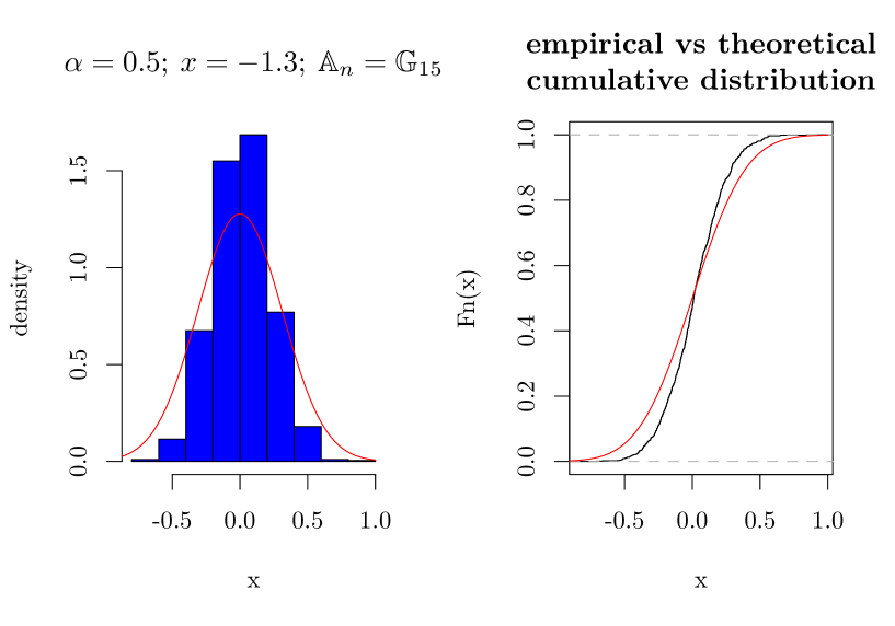
(a) $\alpha=0.5$

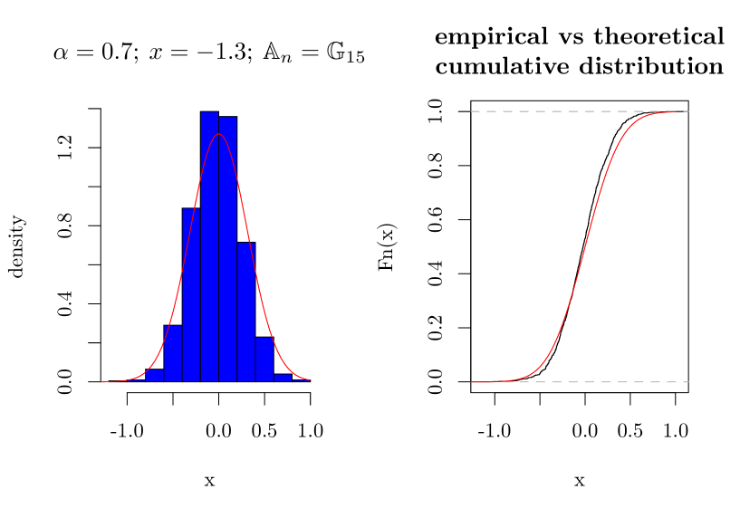
(b) $\alpha=0.7$

Figure 1. Histogram and empirical cumulative distribution of $\zeta_{n}$ given in (20) with $x=-1.3$, $n=15$, ${\mathbb{A}}_{n}=\mathbb{G}_{n}$ and $\gamma=1/5+10^{-3}$. We consider the (sub-critical) ergodic rate of convergence: $\alpha=0.5$ and $\alpha=0.7$.

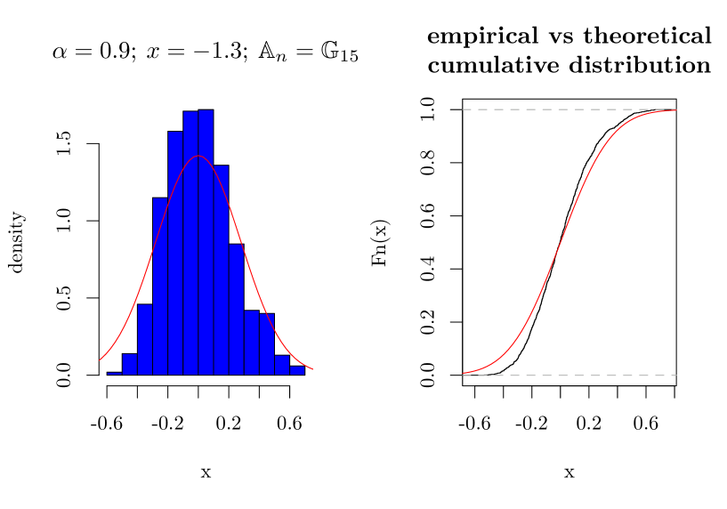
(a) $\gamma=0.696$

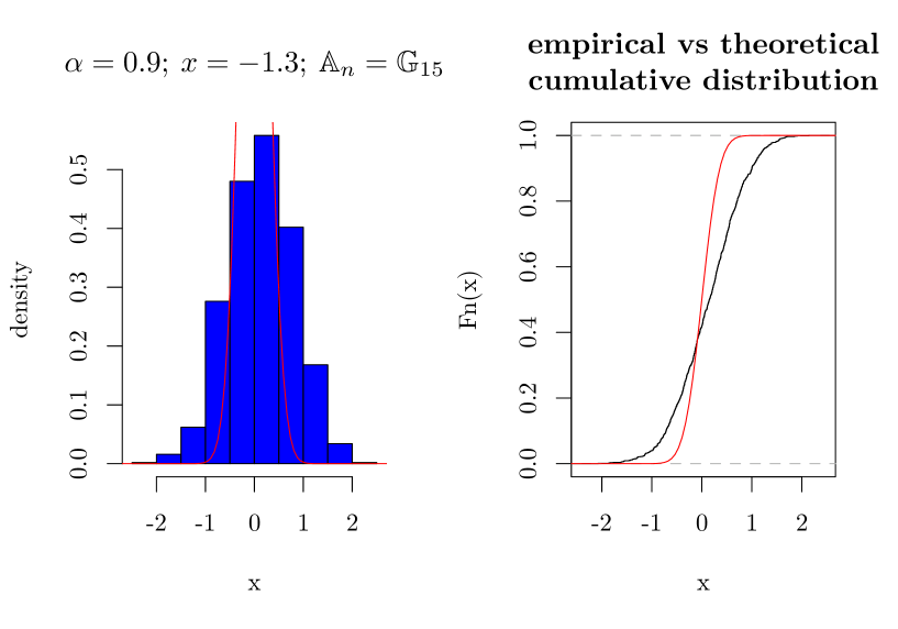
(b) $\gamma=1/5+10^{-3}$

Figure 2. Histogram and empirical cumulative distribution of $\zeta_{n}$ given in (20) with $x=-1.3$, $n=15$, ${\mathbb{A}}_{n}=\mathbb{G}_{n}$ and the ergodic rate $\alpha=0.9$ (super-critical case). We consider the bandwidth exponent $\gamma=0.696$ (which satisfies (14)) for the two left graphics and $\gamma=1/5+10^{-3}$ (which does not satisfy (14)) for the two right.

3.4. A general CLT for additive functionals of BMC

The proof of Lemma 3.5 and Theorem 3.6 rely on a general central limit result for additive functionals of BMC. In the spirit of [1], we introduce the following series of assumptions in a general $L^{2}(\mu)$ framework, with increasing conditions as the geometric ergodic rate $\alpha$ exceed the critical threshold of $1/\sqrt{2}$. In fact, we believe that the general framework presented in this section may be used also for others nonparametric smoothing methods for BMC than the one presented in Section 3.1.

Let $X=(X_{u},u\in\mathbb{T})$ be a BMC on $(S,{\mathscr{S}})$ with initial probability distribution $\nu$, and probability kernel ${\mathcal{P}}$. Recall ${\mathcal{Q}}$ is the induced Markov kernel. In the spirit of Assumption 2.4 and Remark 2.5 in [1], we consider the following hypothesis on asymptotic and non-asymptotic distribution of the process.

Assumption 3.11 ($L^{2}(\mu)$ regularity for the probability kernel ${\mathcal{P}}$ and density of the initial distribution).

There exists an invariant probability measure $\mu$ of ${\mathcal{Q}}$ and:

1. There exists $k_{1}\in{\mathbb{N}}$ and a finite constant $M$ such that for all $f,g\in L^{2}(\mu)$:

   (21) $$\mathop{\parallel\!{\mathcal{P}}({\mathcal{Q}}^{k_{1}}f\otimes{\mathcal{Q}}^{k_{1}}g)\!\parallel}\nolimits_{L^{2}(\mu)}\leq M\mathop{\parallel\!f\!\parallel}\nolimits_{L^{2}(\mu)}\mathop{\parallel\!g\!\parallel}\nolimits_{L^{2}(\mu)},$$

   and for all $h\in L^{2}(\mu)$, and all $m\in\{0,\ldots,k_{1}\}$:

   (22) $$\mathop{\parallel\!{\mathcal{P}}\left({\mathcal{Q}}^{m}{\mathcal{P}}({\mathcal{Q}}^{k_{1}}f\otimes_{\rm sym}{\mathcal{Q}}^{k_{1}}g)\otimes_{\rm sym}{\mathcal{Q}}^{k_{1}}h\right)\!\parallel}\nolimits_{L^{2}(\mu)}\leq M\mathop{\parallel\!f\!\parallel}\nolimits_{L^{2}(\mu)}\mathop{\parallel\!g\!\parallel}\nolimits_{L^{2}(\mu)}\mathop{\parallel\!h\!\parallel}\nolimits_{L^{2}(\mu)}.$$

2. There exists $k_{0}\in{\mathbb{N}}$, such that the probability measure $\nu{\mathcal{Q}}^{k_{0}}$ has a bounded density, say $\nu_{0}$, with respect to $\mu$:

   $$\nu{\mathcal{Q}}^{k_{0}}(dy)=\nu_{0}(y)\mu(dy)\quad\text{and}\quad\mathop{\parallel\!\nu_{0}\!\parallel}\nolimits_{\infty}<+\infty.$$

The next family of three assumptions are related to the sequence of functions which will be considered.

Assumption 3.12 (Regularity of the approximation functions in the sub-critical regime).

Let $(f_{\ell,n},\,n\geq\ell\geq 0)$ be a sequence of real-valued measurable functions defined on $S$ such that:

• There exists $\rho\in(0,1/2)$ such that $\sup_{n\geq\ell\geq 0}2^{-n\rho}\,\|f_{\ell,n}\|_{\infty}$ is finite.

• The constants ${\mathfrak{c}}_{2}=\sup_{n\geq\ell\geq 0}\|f_{\ell,n}\|_{L^{2}(\mu)}$ and ${\mathfrak{q}}_{2}=\sup_{n\geq\ell\geq 0}\mathop{\parallel\!{\mathcal{Q}}(f_{\ell,n}^{2})\!\parallel}\nolimits^{1/2}_{\infty}$ are finite.

• There exists a sequence $(\delta_{\ell,n},n\geq\ell\geq 0)$ of positive numbers such that $\Delta=\sup_{n\geq\ell\geq 0}\delta_{\ell,n}$ is finite, $\lim_{n\rightarrow\infty}\delta_{\ell,n}=0$ for all $\ell\in{\mathbb{N}}$, and for all $n\geq\ell\geq 0$:

  $$\langle\mu,|f_{\ell,n}|\rangle+|\langle\mu,{\mathcal{P}}(f_{\ell,n}\otimes^{2})\rangle|\leq\delta_{\ell,n};$$

  and for all $g\in{\mathcal{B}}_{+}(S)$:

  (23) $$\mathop{\parallel\!{\mathcal{P}}(|f_{\ell,n}|\otimes_{\rm sym}Qg)\!\parallel}\nolimits_{L^{2}(\mu)}\leq\delta_{\ell,n}\mathop{\parallel\!g\!\parallel}\nolimits_{L^{2}(\mu)}.$$

• The following limit exists and is finite:

  (24) $$\sigma^{2}=\lim_{n\rightarrow\infty}\sum_{\ell=0}^{n}2^{-\ell}\mathop{\parallel\!f_{\ell,n}\!\parallel}\nolimits_{L^{2}(\mu)}^{2}<+\infty.$$

Remark 3.13.

We stress that (i) and (ii) of Assumption 3.12 imply the existence of finite constant $C$ such that for all $n\geq\ell\geq 0$:

$$\langle\mu,f_{\ell,n}^{4}\rangle\leq\|f_{\ell,n}\|^{2}_{\infty}\langle\mu,f_{\ell,n}^{2}\rangle\leq C\,{\mathfrak{c}}_{2}^{2}\,2^{2n\rho}\quad\text{and}\quad\langle\mu,f_{\ell,n}^{6}\rangle\leq C\,{\mathfrak{c}}_{2}^{2}\,2^{4n\rho}.$$

We will use the following notations: for $n\in{\mathbb{N}}$, set ${\mathfrak{f}}_{n}=(f_{\ell,n},\ell\in{\mathbb{N}})$ with the convention that $f_{\ell,n}=0$ if $\ell>n$; and for $k\in{\mathbb{N}}^{*}$:

(25) $$c_{k}({\mathfrak{f}}_{n})=\sup_{\ell\geq 0}\mathop{\parallel\!f_{\ell,n}\!\parallel}\nolimits_{L^{k}(\mu)}\quad\text{and}\quad q_{k}({\mathfrak{f}}_{n})=\sup_{\ell\geq 0}\mathop{\parallel\!{\mathcal{Q}}(f_{\ell,n}^{k})\!\parallel}\nolimits_{\infty}^{1/k}.$$

In particular, we have ${\mathfrak{c}}_{2}=\sup_{n\geq 0}c_{2}({\mathfrak{f}}_{n})$ and ${\mathfrak{q}}_{2}=\sup_{n\geq 0}q_{2}({\mathfrak{f}}_{n})$.

For the critical case, $2\alpha^{2}=1$, we shall assume Assumption 3.12 as well as the following.

Assumption 3.14 (Regularity of the approximation functions in the critical regime).

Keeping the same notations as in Assumption 3.12, we further assume that:

• (26) $$\lim_{n\rightarrow\infty}n\sum_{\ell=0}^{n}2^{-\ell/2}\,\delta_{\ell,n}=0.$$

• For all $n\geq\ell\geq 0$:

  (27) $$\|{\mathcal{Q}}(|f_{\ell,n}|)\|_{\infty}\leq\delta_{\ell,n}.$$

For the super-critical case, $2\alpha^{2}>1$, we shall assume Assumptions 3.12, 3.14 as well as the following.

Assumption 3.15 (Regularity of the approximation functions in the super-critical regime).

Keeping the same notations as in Assumption 3.14, we further assume that Assumption 2.4 holds with $2\alpha^{2}>1$ and that:

(28) $$\sup_{0\leq\ell\leq n}(2\alpha^{2})^{n-\ell}\delta_{\ell,n}^{2}<+\infty\quad\text{and, for all $\ell\in{\mathbb{N}}$,}\quad\lim_{n\rightarrow\infty}(2\alpha^{2})^{n-\ell}\delta_{\ell,n}^{2}=0.$$

Notice that condition (28) implies (26) as well as $\Delta<+\infty$ and $\lim_{n\rightarrow\infty}\delta_{\ell,n}=0$ for all $\ell\in{\mathbb{N}}$ (see Assumption 3.12 (iii)) when $2\alpha^{2}>1$.

Following [1], for a finite set ${\mathbb{A}}\subset\mathbb{T}$ and a function $f\in{\mathcal{B}}(S)$, we set:

(29) $$M_{\mathbb{A}}(f)=\sum_{i\in{\mathbb{A}}}f(X_{i}).$$

We shall be interested in the cases ${\mathbb{A}}=\mathbb{G}_{n}$ (the $n$-th generation) and ${\mathbb{A}}=\mathbb{T}_{n}$ (the tree up to the $n$-th generation). We shall assume that $\mu$ is an invariant probability measure of ${\mathcal{Q}}$. In view of Remark 2.3, one is interested in the fluctuations of $|\mathbb{G}_{n}|^{-1}\,M_{\mathbb{G}_{n}}(f)$ around $\langle\mu,f\rangle$. So, we will use frequently the following notation:

(30) $$\boxed{\tilde{f}=f-\langle\mu,f\rangle\quad\text{for $f\in L^{1}(\mu)$.}}$$

Let ${\mathfrak{f}}=(f_{\ell},\ell\in{\mathbb{N}})$ be a sequence of elements of $L^{1}(\mu)$. We set for $n\in{\mathbb{N}}$:

(31) $$\boxed{N_{n,\emptyset}({\mathfrak{f}})=|\mathbb{G}_{n}|^{-1/2}\sum_{\ell=0}^{n}M_{\mathbb{G}_{n-\ell}}(\tilde{f}_{\ell}).}$$

The notation $N_{n,\emptyset}$ means that we consider the average from the root $\emptyset$ up to the $n$-th generation.

Remark 3.16.

The following two simple cases are frequently used in the literature. Let $f\in L^{1}(\mu)$ and consider the sequence ${\mathfrak{f}}=(f_{\ell},\ell\in{\mathbb{N}})$. If $f_{0}=f$ and $f_{\ell}=0$ for $\ell\in{\mathbb{N}}^{*}$, then we get:

$$N_{n,\emptyset}({\mathfrak{f}})=|\mathbb{G}_{n}|^{-1/2}M_{\mathbb{G}_{n}}(\tilde{f}).$$

If $f_{\ell}=f$ for $\ell\in{\mathbb{N}}$, then we get, as $|\mathbb{T}_{n}|=2^{n+1}-1$ and $|\mathbb{G}_{n}|=2^{n}$:

$$N_{n,\emptyset}({\mathfrak{f}})=|\mathbb{G}_{n}|^{-1/2}M_{\mathbb{T}_{n}}(\tilde{f})=\sqrt{2-2^{-n}}\,\,|\mathbb{T}_{n}|^{-1/2}M_{\mathbb{T}_{n}}(\tilde{f}).$$

Thus, we will easily deduce the fluctuations of $M_{\mathbb{T}_{n}}(f)$ and $M_{\mathbb{G}_{n}}(f)$ from the asymptotics of $N_{n,\emptyset}({\mathfrak{f}})$.

The main result of this section is motivated by the decomposition given in (8). It will allow us to treat the variance term of kernel estimators defined in (7). The proof is given in Section 5 for the sub-critical case ($\alpha\in(0,1/\sqrt{2})$), in Section 6 for the critical case ($\alpha=1/\sqrt{2}$) and in Section 7 for the supercritical case ($\alpha\in(1/\sqrt{2},1)$), with $\alpha$ the rate defined in Assumption 2.4. Recall $N_{n,\emptyset}({\mathfrak{f}})$ defined in (31).

Theorem 3.17.

Let $X$ be a BMC with kernel ${\mathcal{P}}$ and initial distribution $\nu$, such that Assumption 2.4 (on the geometric ergodic rate $\alpha\in(0,1)$), Assumption 3.11 (on the regularity of ${\mathcal{P}}$ and of $\nu$) and Assumption 3.12 (on the approximation functions $(f_{\ell,n},n\geq\ell\geq 0)$) are in force.

Furthermore, if $\alpha=1/\sqrt{2}$ then assume that Assumption 3.14 holds; and if $\alpha>1/\sqrt{2}$ then assume that Assumption 3.14 and Assumption 3.15 hold. Then, we have the following convergence in distribution:

$$N_{n,\emptyset}({\mathfrak{f}}_{n})\;\xrightarrow[n\rightarrow\infty]{\text{(d)}}\;G,$$

where ${\mathfrak{f}}_{n}=(f_{\ell,n},\,\ell\in{\mathbb{N}})$ and the convention that $f_{\ell,n}=0$ for $\ell>n$, and with $G$ a centered Gaussian random variable with finite variance $\sigma^{2}$ defined in (24).

Remark 3.18.

Assume $\sigma^{2}_{\ell}=\lim_{n\rightarrow\infty}\mathop{\parallel\!f_{\ell,n}\!\parallel}\nolimits_{L^{2}(\mu)}^{2}$ exists for all $\ell\in{\mathbb{N}}$; so that $\sigma^{2}$ defined in (24) is also equal to $\sum_{\ell\in{\mathbb{N}}}2^{-\ell}\sigma^{2}_{\ell}$. According to additive form of the variance $\sigma^{2}$, we deduce that for fixed $k\in{\mathbb{N}}$, the random variables $\left(|\mathbb{G}_{n}|^{-1/2}M_{\mathbb{G}_{n-\ell}}(\tilde{f}_{\ell,n}),\,\ell\in\{0,\ldots,k\}\right)$ converges in distribution, as $n$ goes to infinity towards $(G_{\ell},\,\ell\in\{0,\ldots,k\})$ which are independent real-valued Gaussian centered random variables with variance ${\mathrm{Var}}(G_{\ell})=2^{-\ell}\sigma^{2}_{\ell}$.

4. Proof of Lemma 3.5 and Theorem 3.6

4.1. Checking Assumptions 3.11, 3.12, 3.14 and 3.15

We shall check that Assumptions 3.1, 3.2 and 3.3, and Equation (14), for the density estimation, implies the more general Assumptions 3.11, 3.12, 3.14 and 3.15.

We check that Assumption 3.1 implies Assumption 3.11 on the $L^{2}(\mu)$ regularity for the probability kernel ${\mathcal{P}}$ and density of the initial distribution. Notice that Assumption 3.1 (iv) and Assumption 3.11 (ii) coincide. So, it is enough to check that Assumption 3.1 (i)-(iii) implies Assumption 3.11 (i). Since $|{\mathcal{Q}}f|\leq\mathop{\parallel\!f\!\parallel}\nolimits_{L^{2}(\mu)}{\mathfrak{h}}$, we deduce that $|{\mathcal{Q}}^{k_{1}}f|\leq\mathop{\parallel\!f\!\parallel}\nolimits_{L^{2}(\mu)}{\mathfrak{h}}_{k_{1}}$. We deduce that:

$$\mathop{\parallel\!{\mathcal{P}}({\mathcal{Q}}^{k_{1}}f\otimes{\mathcal{Q}}^{k_{1}}g)\!\parallel}\nolimits_{L^{2}(\mu)}\leq\mathop{\parallel\!f\!\parallel}\nolimits_{L^{2}(\mu)}\mathop{\parallel\!g\!\parallel}\nolimits_{L^{2}(\mu)}\mathop{\parallel\!{\mathcal{P}}({\mathfrak{h}}_{k_{1}}\otimes^{2})\!\parallel}\nolimits_{L^{2}(\mu)}.$$

Then use (3) to get that $\mathop{\parallel\!{\mathcal{P}}({\mathfrak{h}}_{k_{1}}\otimes^{2})\!\parallel}\nolimits_{L^{2}(\mu)}\leq\mathop{\parallel\!{\mathcal{Q}}\left({\mathfrak{h}}_{k_{1}}^{2}\right)\!\parallel}\nolimits_{L^{2}(\mu)}\leq\mathop{\parallel\!{\mathfrak{h}}_{k_{1}}^{2}\!\parallel}\nolimits_{L^{2}(\mu)}\leq\mathop{\parallel\!{\mathfrak{h}}_{k_{1}}\!\parallel}\nolimits^{2}_{L^{6}(\mu)}<+\infty$. This gives (21). Similarly, we have:

$$\mathop{\parallel\!{\mathcal{P}}\left({\mathcal{Q}}^{m}{\mathcal{P}}({\mathcal{Q}}^{k_{1}}f\otimes_{\rm sym}{\mathcal{Q}}^{k_{1}}g)\otimes_{\rm sym}{\mathcal{Q}}^{k_{1}}h\right)\!\parallel}\nolimits_{L^{2}(\mu)}\\ \leq\mathop{\parallel\!f\!\parallel}\nolimits_{L^{2}(\mu)}\mathop{\parallel\!g\!\parallel}\nolimits_{L^{2}(\mu)}\mathop{\parallel\!h\!\parallel}\nolimits_{L^{2}(\mu)}\mathop{\parallel\!{\mathcal{P}}\left({\mathcal{Q}}^{m}{\mathcal{P}}({\mathfrak{h}}_{k_{1}}\otimes^{2})\otimes_{\rm sym}{\mathfrak{h}}_{k_{1}}\right)\!\parallel}\nolimits_{L^{2}(\mu)}.$$

On the other hand, using (5), the Hölder inequality and (3), we also have:

$$\mathop{\parallel\!{\mathcal{P}}\left({\mathcal{Q}}^{m}{\mathcal{P}}(f_{0}\otimes^{2})\otimes_{\rm sym}g_{0}\right)\!\parallel}\nolimits_{L^{2}(\mu)}^{2} \leq 4\langle\mu,{\mathcal{Q}}(({\mathcal{Q}}^{m}{\mathcal{P}}(f_{0}\otimes^{2}))^{2}){\mathcal{Q}}(g_{0}^{2})\rangle$$

$$\leq 4\langle\mu,{\mathcal{P}}(f_{0}\otimes^{2})^{3}\rangle^{2/3}\langle\mu,{\mathcal{Q}}(g_{0}^{2})^{3}\rangle^{1/3}$$

$$\leq 4\langle\mu,f_{0}^{6}\rangle^{2/3}\langle\mu,g_{0}^{6}\rangle^{1/3}.$$

Taking $f_{0}=g_{0}={\mathfrak{h}}_{k_{1}}$ gives that $\mathop{\parallel\!{\mathcal{P}}\left({\mathcal{Q}}^{m}{\mathcal{P}}({\mathfrak{h}}_{k_{1}}\otimes^{2})\otimes_{\rm sym}{\mathfrak{h}}_{k_{1}}\right)\!\parallel}\nolimits_{L^{2}(\mu)}\leq 2\mathop{\parallel\!{\mathfrak{h}}_{k_{1}}\!\parallel}\nolimits_{L^{6}}^{3}<+\infty$. This gives (22). Thus, Assumption 3.11 (i) holds.

We suppose that $S={\mathbb{R}}^{d}$ and that Assumptions 3.1, 3.2 hold. Let $K$ be a kernel function satisfying Assumption 3.3 (i) and bandwidths $(h_{n},n\in{\mathbb{N}})$ satisfying Assumption 3.3 (ii). For $x\in S$, we define the sequences of functions $(f^{x}_{\ell},\,\ell\in{\mathbb{N}})$ given by:

$$f^{x}_{\ell}(y)=K_{h_{\ell}}(x-y)={h_{\ell}^{-d/2}}K\left(\frac{x-y}{h_{\ell}}\right)\quad\text{for $y\in{\mathbb{R}}^{d}$}.$$

Then, we consider the sequences of functions $(f_{\ell,n}^{\text{shift}},\,n\geq\ell\geq 0)$, $(f_{\ell,n}^{\text{id}},\,n\geq\ell\geq 0)$ and $(f^{0}_{\ell,n},\,n\geq\ell\geq 0)$ defined by:

(32) $$f_{\ell,n}^{\text{shift}}=f^{x}_{n-\ell},\quad f_{\ell,n}^{\text{id}}=f^{x}_{n}\quad\text{and}\quad f^{0}_{\ell,n}=f^{x}_{n}{\bf 1}_{\{\ell=0\}}.$$

Under those hypothesis, we shall check that Assumptions 3.12, 3.14 and 3.15 hold for those three sequences of functions. We first check that (i-iii) from Assumption 3.12 and (v-vi) from Assumption 3.14. We consider only the sequence $(f_{\ell,n},\,n\geq\ell\geq 0)$ with $f_{\ell,n}=f_{\ell,n}^{\text{shift}}$, the arguments for the other two being similar. We have $\mathop{\parallel\!f_{\ell,n}\!\parallel}\nolimits_{\infty}=h_{n-\ell}^{-d/2}\mathop{\parallel\!K\!\parallel}\nolimits_{\infty}=2^{(n-\ell)d\gamma/2}\mathop{\parallel\!K\!\parallel}\nolimits_{\infty}$. Thus property (i) of Assumption 3.12 holds with $\rho=d\gamma/2$. We have:

$$\mathop{\parallel\!f_{\ell,n}\!\parallel}\nolimits_{1}=h_{n-\ell}^{d/2}\mathop{\parallel\!K\!\parallel}\nolimits_{1}=2^{-(n-\ell)d\gamma/2}\mathop{\parallel\!K\!\parallel}\nolimits_{1}\quad\text{and}\quad\mathop{\parallel\!f_{\ell,n}\!\parallel}\nolimits_{2}=\mathop{\parallel\!K\!\parallel}\nolimits_{2}.$$

This gives $\mathop{\parallel\!f_{\ell,n}\!\parallel}\nolimits_{L^{2}(\mu)}^{2}\leq\mathop{\parallel\!f_{\ell,n}\!\parallel}\nolimits^{2}_{2}\,\mathop{\parallel\!\mu\!\parallel}\nolimits_{\infty}\leq C_{0}\mathop{\parallel\!K\!\parallel}\nolimits_{2}^{2}$ and

$$\mathop{\parallel\!{\mathcal{Q}}(f_{\ell,n}^{2})\!\parallel}\nolimits_{\infty}\leq\mathop{\parallel\!f_{\ell,n}\!\parallel}\nolimits^{2}_{2}\,\sup_{x,y\in{\mathbb{R}}^{d}}q(x,y)\mu(y)\leq C_{0}\mathop{\parallel\!K\!\parallel}\nolimits_{2}^{2}.$$

We conclude that (ii) of Assumption 3.12 holds with ${\mathfrak{c}}_{2}={\mathfrak{q}}_{2}=C_{0}^{1/2}\mathop{\parallel\!K\!\parallel}\nolimits_{2}$. We have $\langle\mu,|f_{\ell,n}|\rangle\leq C_{0}\mathop{\parallel\!K\!\parallel}\nolimits_{1}h_{n-\ell}^{d/2}$ and $|\langle\mu,{\mathcal{P}}(f_{\ell,n}\otimes^{2})\rangle|\leq C_{1}\mathop{\parallel\!K\!\parallel}\nolimits_{1}^{2}h_{n-\ell}^{d}$. Furthermore, for all $g\in{\mathcal{B}}_{+}(\mathbb{R}^{d})$, we have $\mathop{\parallel\!{\mathcal{P}}(|f_{\ell,n}|\otimes_{\rm sym}Qg)\!\parallel}\nolimits_{L^{2}(\mu)}\leq C_{2}h_{n-\ell}^{d/2}\mathop{\parallel\!K\!\parallel}\nolimits_{1}\mathop{\parallel\!g\!\parallel}\nolimits_{L^{2}(\mu)}$. We also have $\mathop{\parallel\!{\mathcal{Q}}(|f_{\ell,n}|)\!\parallel}\nolimits_{\infty}\leq C_{0}\mathop{\parallel\!K\!\parallel}\nolimits_{1}h_{n-\ell}^{d/2}$. This implies that (iii) of Assumption 3.12 and (vi) of Assumption 3.14 hold with $\delta_{\ell,n}=c\,h_{n-\ell}^{d/2}=c2^{-(n-\ell)d\gamma/2}$ for some finite constant $c$ depending only on $C_{0},C_{1},C_{2}$ and $\mathop{\parallel\!K\!\parallel}\nolimits_{1}$. With this choice of $\delta_{\ell,n}$, notice that (v) of Assumption 3.14 also holds as $d\gamma<1$.

Recall that $d\gamma<1$. Moreover, if Equation (14) holds,, that is $2^{d\gamma}>2\alpha^{2}$ where $\alpha$ is the rate given in Assumption 2.4 (this is restrictive on $\gamma$ only in the super-critical regime $2\alpha^{2}>1$), then Assumption 3.15 also holds with the latter choice of $\delta_{\ell,n}.$

Eventually we prove (iv) of Assumption 3.12. We recall the following result due to Bochner (see [15, Theorem 1A] which can be easily extended to any dimension $d\geq 1$).

Lemma 4.1.

Let $(h_{n},n\in\mathbb{N})$ be a sequence of positive numbers converging to $0$ as $n$ goes to infinity. Let $g:\mathbb{R}^{d}\rightarrow\mathbb{R}$ be a measurable function such that $\int_{\mathbb{R}^{d}}|g(x)|dx<+\infty$. Let $f:\mathbb{R}^{d}\rightarrow\mathbb{R}$ be a measurable function such that $\mathop{\parallel\!f\!\parallel}\nolimits_{\infty}<+\infty$, $\int_{{\mathbb{R}}^{d}}|f(y)|\,dy<+\infty$ and $\lim_{|x|\rightarrow+\infty}|x|f(x)=0$. Define

$$g_{n}(x)=h_{n}^{-d}\int_{\mathbb{R}^{d}}f(h_{n}^{-1}(x-y))g(y)dy.$$

Then, we have at every point $x$ of continuity of $g$,

$$\lim_{n\rightarrow+\infty}g_{n}(x)=g(x)\int_{\mathbb{R}}f(y)dy.$$

Let $x$ be in the set of continuity of $\mu$. Thanks to Lemma 4.1, we have:

$$\lim_{\ell\rightarrow\infty}\mathop{\parallel\!f^{x}_{\ell}\!\parallel}\nolimits_{L^{2}(\mu)}^{2}=\lim_{\ell\rightarrow\infty}\langle\mu,(f^{x}_{\ell})^{2}\rangle=\mu(x)\mathop{\parallel\!K\!\parallel}\nolimits_{2}^{2}.$$

We deduce that the sequences of functions $(f_{\ell,n}^{\text{shift}},\,n\geq\ell\geq 0)$, $(f_{\ell,n}^{\text{id}},\,n\geq\ell\geq 0)$ and $(f^{0}_{\ell,n},\,n\geq\ell\geq 0)$ satisfy (iv) of Assumption 3.12 with $\sigma^{2}$ defined by (24) respectively given by:

(33) $$(\sigma^{\text{shift}})^{2}=2\mu(x)\mathop{\parallel\!K\!\parallel}\nolimits_{2}^{2},\,\quad(\sigma^{\text{id}})^{2}=2\mu(x)\mathop{\parallel\!K\!\parallel}\nolimits_{2}^{2}\,\quad\text{and}\quad(\sigma^{0})^{2}=\mu(x)\mathop{\parallel\!K\!\parallel}\nolimits_{2}^{2}.$$

4.2. Proof of Lemma 3.5

We begin the proof with ${\mathbb{A}}_{n}=\mathbb{T}_{n}.$ We have the following decomposition:

(34) $$\widehat{\mu}_{\mathbb{T}_{n}}(x)-\mu(x)=\frac{\sqrt{|\mathbb{G}_{n}|}}{|\mathbb{T}_{n}|h_{n}^{d/2}}N_{n,\emptyset}({\mathfrak{f}}_{n})+B_{h_{n}}(x),$$

where ${\mathfrak{f}}_{n}=(f_{\ell,n},\,\ell\in{\mathbb{N}})$ with the functions $f_{\ell,n}=f_{\ell,n}^{\text{id}}$ defined in (32) for $n\geq\ell\geq 0$ and $f_{\ell,n}=0$ otherwise; $N_{n,\emptyset}$ is defined in (31) with ${\mathfrak{f}}$ replaced by ${\mathfrak{f}}_{n}$; and the bias term:

$$B_{h_{n}}(x)=\frac{1}{|\mathbb{T}_{n}|h_{n}^{d/2}}\sum_{\ell=0}^{n}2^{n-\ell}\langle\mu,f_{\ell,n}\rangle-\mu(x)=\langle\mu,h_{n}^{-d}K(h_{n}^{-1}(x-\cdot))\rangle-\mu(x).$$

Thanks to Section 4.1, we have under the assumption of Lemma 3.5 that Assumptions 3.11, 3.12, 3.14 and 3.15 hold. Since $\lim_{n\rightarrow\infty}|\mathbb{G}_{n}|h_{n}^{d}=\infty$ as $\gamma<1$, we get that $\lim_{n\rightarrow\infty}|\mathbb{G}_{n}|^{1/2}/|\mathbb{T}_{n}|h_{n}^{d/2}=0$. Thus, we get, as a direct consequence of Theorem 3.17 the following convergence in probability:

$$\lim_{n\rightarrow\infty}\frac{\sqrt{|\mathbb{G}_{n}|}}{|\mathbb{T}_{n}|h_{n}^{d/2}}N_{n,\emptyset}({\mathfrak{f}}_{n})=0.$$

Next, it follows from Lemma 4.1 that $\lim_{n\rightarrow\infty}B_{h_{n}}(x)=0$. By considering the functions $f_{\ell,n}=f_{\ell,n}^{0}$ defined in (32), we similarly get the result for the case ${\mathbb{A}}_{n}=\mathbb{G}_{n}$.

4.3. Proof of Theorem 3.6

The sub-critical case and ${\mathbb{A}}_{n}=\mathbb{T}_{n}$. We keep notations from the proof of Lemma 3.5. Recall that ${\mathfrak{f}}_{n}=(f_{\ell,n},\,\ell\in{\mathbb{N}})$ with the functions $f_{\ell,n}=f_{\ell,n}^{\text{id}}$ defined in (32). Using the value of $\sigma=\sigma^{\text{id}}$ in (33), thanks to Theorem 3.17 and the decomposition (34), we see that to get the asymptotic normality of the estimator (15) it suffices to prove that:

(35) $$\lim_{n\rightarrow\infty}|\mathbb{T}_{n}|^{1/2}h_{n}^{d/2}B_{h_{n}}(x)=0.$$

Using that

$$\mu(x-h_{n}y)-\mu(x)=\sum_{j=1}^{d}(\mu(x_{1}-h_{n}y_{1},\ldots,x_{j}-h_{n}y_{j},x_{j+1},\ldots,x_{d})\\ -\mu(x_{1}-h_{n}y_{1},\ldots,x_{j-1}-h_{n}y_{j-1},x_{j},x_{j+1},\ldots,x_{d})),$$

the Taylor expansion and Assumption 3.4, we get that, for some finite constant $C>0$,

$$|\mathbb{T}_{n}|^{1/2}h_{n}^{d/2}B_{h_{n}}(x) =\sqrt{|\mathbb{T}_{n}|h_{n}^{d}}\,\,\Big{|}\int_{\mathbb{R}^{d}}h_{n}^{-d}K(h_{n}^{-1}(x-y))\mu(y)dy-\mu(x)\Big{|}$$

$$=\sqrt{|\mathbb{T}_{n}|h_{n}^{d}}\,\,\Big{|}\int_{\mathbb{R}^{d}}K(y)(\mu(x-h_{n}y)-\mu(x))\,dy\Big{|}$$

$$\leq C\sqrt{|\mathbb{T}_{n}|h_{n}^{d}}\,\,\sum_{j=1}^{d}\,\,\int_{\mathbb{R}^{d}}K(y)\frac{(h_{n}|y_{j}|)^{s}}{\lfloor s\rfloor!}dy$$

$$\leq C\sqrt{|\mathbb{T}_{n}|h_{n}^{2s+d}}.$$

Then Equation (35) follows, since $\lim_{n\rightarrow\infty}|\mathbb{G}_{n}|s_{n}^{2s+d}=0$. This ends the proof for ${\mathbb{A}}_{n}=\mathbb{T}_{n}$.

The sub-critical case and ${\mathbb{A}}_{n}=\mathbb{G}_{n}$. The proof is similar, using instead the functions $f_{\ell,n}=f_{\ell,n}^{0}$ defined in (32).

The critical and super-critical cases. The proof follows the same lines, using Theorem 3.17 in the critical and super-critical cases and the decomposition (34).

5. Proof of Theorem 3.17 in the sub-critical case ($2\alpha^{2}<1$)

Recall the definition of $M_{\mathbb{A}}$ given in (29) and of $\tilde{f}=f-\langle\mu,f\rangle$ in (30). In order to study the asymptotics of $M_{\mathbb{G}_{n-\ell}}(\tilde{f})$ as $n$ goes to infinity and $\ell$ is fixed, it is convenient to consider the contribution of the descendants of the individual $i\in\mathbb{T}_{n-\ell}$ for $n\geq\ell\geq 0$:

(36) $$N^{\ell}_{n,i}(f)=|\mathbb{G}_{n}|^{-1/2}M_{i\mathbb{G}_{n-|i|-\ell}}(\tilde{f}),$$

where $i\mathbb{G}_{n-|i|-\ell}=\{ij,\,j\in\mathbb{G}_{n-|i|-\ell}\}\subset\mathbb{G}_{n-\ell}$. For all $k\in{\mathbb{N}}$ such that $n\geq k+\ell$, we have:

$$M_{\mathbb{G}_{n-\ell}}(\tilde{f})=\sqrt{|\mathbb{G}_{n}|}\,\,\sum_{i\in\mathbb{G}_{k}}N^{\ell}_{n,i}(f)=\sqrt{|\mathbb{G}_{n}|}\,\,N_{n,\emptyset}^{\ell}(f).$$

Let ${\mathfrak{f}}=(f_{\ell},\ell\in{\mathbb{N}})$ be a sequence of elements of $L^{1}(\mu)$. We set for $n\in{\mathbb{N}}$ and $i\in\mathbb{T}_{n}$:

(37) $$N_{n,i}({\mathfrak{f}})=\sum_{\ell=0}^{n-|i|}N_{n,i}^{\ell}(f_{\ell})=|\mathbb{G}_{n}|^{-1/2}\sum_{\ell=0}^{n-|i|}M_{i\mathbb{G}_{n-|i|-\ell}}(\tilde{f}_{\ell}).$$

We deduce that $\sum_{i\in\mathbb{G}_{k}}N_{n,i}({\mathfrak{f}})=|\mathbb{G}_{n}|^{-1/2}\sum_{\ell=0}^{n-k}M_{\mathbb{G}_{n-\ell}}(\tilde{f}_{\ell})$. For $k=0$, we recover Equation (31).

We consider the notations of Theorem 3.17. Recall that ${\mathfrak{f}}_{n}=(f_{\ell,n},\,\ell\in{\mathbb{N}})$ with the convention that $f_{\ell,n}=0$ for $\ell>n$. In the following proofs, we will denote by $C$ any unimportant finite constant which may vary from line to line (in particular $C$ does not depend on $n$ nor on ${\mathfrak{f}}_{n}$).

Remark 5.1.

Recall $k_{0}$ given in Assumption 3.11 (iii). Recall that from Assumption 3.12 (ii), the sequence ${\mathfrak{f}}_{n}$ is bounded in $L^{2}(\mu)$. We have

(38) $$N_{n,\emptyset}({\mathfrak{f}}_{n})=N_{n,\emptyset}^{[k_{0}]}({\mathfrak{f}}_{n})\,+\,|\mathbb{G}_{n}|^{-1/2}\sum_{\ell=0}^{k_{0}-1}M_{\mathbb{G}_{\ell}}(\tilde{f}_{n-\ell,n}),$$

where we set:

$$\boxed{N_{n,\emptyset}^{[k_{0}]}({\mathfrak{f}}_{n})=|\mathbb{G}_{n}|^{-1/2}\sum_{\ell=0}^{n-k_{0}}M_{\mathbb{G}_{n-\ell}}(\tilde{f}_{\ell,n}).}$$

Using the Cauchy-Schwartz inequality, we get

(39) $$|\mathbb{G}_{n}|^{-1/2}|\sum_{\ell=0}^{k_{0}-1}M_{\mathbb{G}_{\ell}}(\tilde{f}_{n-\ell,n})|\leq Cc_{2}({\mathfrak{f}})|\mathbb{G}_{n}|^{-1/2}\,+\,|\mathbb{G}_{n}|^{-1/2}\sum_{\ell=0}^{k_{0}-1}M_{\mathbb{G}_{\ell}}(|f_{n-\ell,n}|).$$

Since the sequence ${\mathfrak{f}}_{n}$ is bounded in $L^{2}(\mu)$ and since $k_{0}$ is finite, we have, for all $\ell\in\{0,\ldots,k_{0}-1\}$, $\lim_{n\rightarrow\infty}|\mathbb{G}_{n}|^{-1/2}M_{\mathbb{G}_{\ell}}(|f_{n-\ell,n}|)=0$ a.s. and then that (used (39))

$$\lim_{n\rightarrow\infty}|\mathbb{G}_{n}|^{-1/2}|\sum_{\ell=0}^{k_{0}-1}M_{\mathbb{G}_{\ell}}(\tilde{f}_{n-\ell})|=0\quad\text{a.s.}$$

Therefore, from (38), the study of $N_{n,\emptyset}({\mathfrak{f}}_{n})$ is reduced to that of $N^{[k_{0}]}_{n,\emptyset}({\mathfrak{f}}_{n})$.

Let $(p_{n},n\in{\mathbb{N}})$ be a non-decreasing sequence of elements of ${\mathbb{N}}^{*}$ such that, for all $\lambda>0$:

(40) $$p_{n}<n,\quad\lim_{n\rightarrow\infty}p_{n}/n=1\quad\text{and}\quad\lim_{n\rightarrow\infty}n-p_{n}-\lambda\log(n)=+\infty.$$

When there is no ambiguity, we write $p$ for $p_{n}$.

Let $i,j\in\mathbb{T}$. We write $i\preccurlyeq j$ if $j\in i\mathbb{T}$. We denote by $i\wedge j$ the most recent common ancestor of $i$ and $j$, which is defined as the only $u\in\mathbb{T}$ such that if $v\in\mathbb{T}$ and $v\preccurlyeq i$, $v\preccurlyeq j$ then $v\preccurlyeq u$. We also define the lexicographic order $i\leq j$ if either $i\preccurlyeq j$ or $v0\preccurlyeq i$ and $v1\preccurlyeq j$ for $v=i\wedge j$. Let $X=(X_{i},i\in\mathbb{T})$ be a $BMC$ with kernel ${\mathcal{P}}$ and initial measure $\nu$. For $i\in\mathbb{T}$, we define the $\sigma$-field:

$${\mathcal{F}}_{i}=\{X_{u};u\in\mathbb{T}\text{ such that $u\leq i$}\}.$$

By construction, the $\sigma$-fields $({\mathcal{F}}_{i};\,i\in\mathbb{T})$ are nested as ${\mathcal{F}}_{i}\subset{\mathcal{F}}_{j}$ for $i\leq j$.

We define for $n\in{\mathbb{N}}$, $i\in\mathbb{G}_{n-p_{n}}$ and ${\mathfrak{f}}_{n}$ the martingale increments:

(41) $$\Delta_{n,i}({\mathfrak{f}}_{n})=N_{n,i}({\mathfrak{f}}_{n})-{\mathbb{E}}\left[N_{n,i}({\mathfrak{f}}_{n})|\,{\mathcal{F}}_{i}\right]\quad\text{and}\quad\Delta_{n}({\mathfrak{f}}_{n})=\sum_{i\in\mathbb{G}_{n-p_{n}}}\Delta_{n,i}({\mathfrak{f}}_{n}).$$

Thanks to (37), we have:

$$\sum_{i\in\mathbb{G}_{n-p_{n}}}N_{n,i}({\mathfrak{f}}_{n})=|\mathbb{G}_{n}|^{-1/2}\sum_{\ell=0}^{p_{n}}M_{\mathbb{G}_{n-\ell}}(\tilde{f}_{\ell,n})=|\mathbb{G}_{n}|^{-1/2}\sum_{k=n-p_{n}}^{n}M_{\mathbb{G}_{k}}(\tilde{f}_{n-k,n}).$$

Using the branching Markov property, and (37), we get for $i\in\mathbb{G}_{n-p_{n}}$:

$${\mathbb{E}}\left[N_{n,i}({\mathfrak{f}}_{n})|\,{\mathcal{F}}_{i}\right]={\mathbb{E}}\left[N_{n,i}({\mathfrak{f}}_{n})|\,X_{i}\right]=|\mathbb{G}_{n}|^{-1/2}\sum_{\ell=0}^{p_{n}}{\mathbb{E}}_{X_{i}}\left[M_{\mathbb{G}_{p_{n}-\ell}}(\tilde{f}_{\ell,n})\right].$$

Assume that $n$ is large enough so that $n-p_{n}-1\geq k_{0}$. We have:

$$N^{[k_{0}]}_{n,\emptyset}({\mathfrak{f}})=\Delta_{n}({\mathfrak{f}})+R_{0}^{k_{0}}(n)+R_{1}(n),$$

where $\Delta_{n}({\mathfrak{f}})$ and $R_{1}(n)$ are defined in (41) and:

$$R_{0}^{k_{0}}(n)=|\mathbb{G}_{n}|^{-1/2}\,\sum_{k=k_{0}}^{n-p_{n}-1}M_{\mathbb{G}_{k}}(\tilde{f}_{n-k})\quad\text{and}\quad R_{1}(n)=\sum_{i\in\mathbb{G}_{n-p_{n}}}{\mathbb{E}}\left[N_{n,i}({\mathfrak{f}}_{n})|\,{\mathcal{F}}_{i}\right].$$

We have the following result:

Lemma 5.2.

Under the assumptions of Theorem 3.17 ($2\alpha^{2}<1$), we have that

$$\lim_{n\rightarrow\infty}{\mathbb{E}}\left[\left(N^{[k_{0}]}_{n,\emptyset}({\mathfrak{f}}_{n})-\Delta_{n}({\mathfrak{f}}_{n})\right)^{2}\right]=0.$$

Proof.

We deduce from Remark 5.5 in [1] that ${\mathbb{E}}\left[\left(N^{[k_{0}]}_{n,\emptyset}({\mathfrak{f}}_{n})-\Delta_{n}({\mathfrak{f}}_{n})\right)^{2}\right]\leq a_{0,n}\,{\mathfrak{c}}_{2}^{2}$ for a sequence $(a_{0,n},n\in{\mathbb{N}})$ which converges to $0$ and does not depend on the sequences ${\mathfrak{f}}_{n}$. ∎

We consider the bracket of the martingale $\Delta_{n}({\mathfrak{f}}_{n})$ given by $V(n)=\sum_{i\in\mathbb{G}_{n-p_{n}}}{\mathbb{E}}\left[\Delta_{n,i}({\mathfrak{f}}_{n})^{2}|{\mathcal{F}}_{i}\right]$. Using (37) and (41), we write:

(42) $$V(n)=|\mathbb{G}_{n}|^{-1}\sum_{i\in\mathbb{G}_{n-p_{n}}}{\mathbb{E}}_{X_{i}}\left[\left(\sum_{\ell=0}^{p_{n}}M_{\mathbb{G}_{p_{n}-\ell}}(\tilde{f}_{\ell,n})\right)^{2}\right]-R_{2}(n)=V_{1}(n)+2V_{2}(n)-R_{2}(n),$$

with:

$$V_{1}(n) =|\mathbb{G}_{n}|^{-1}\sum_{i\in\mathbb{G}_{n-p_{n}}}\sum_{\ell=0}^{p_{n}}{\mathbb{E}}_{X_{i}}\left[M_{\mathbb{G}_{p_{n}-\ell}}(\tilde{f}_{\ell,n})^{2}\right],$$

$$V_{2}(n) =|\mathbb{G}_{n}|^{-1}\sum_{i\in\mathbb{G}_{n-p_{n}}}\sum_{0\leq\ell<k\leq p_{n}}{\mathbb{E}}_{X_{i}}\left[M_{\mathbb{G}_{p_{n}-\ell}}(\tilde{f}_{\ell,n})M_{\mathbb{G}_{p_{n}-k}}(\tilde{f}_{k,n})\right],$$

$$R_{2}(n) =\sum_{i\in\mathbb{G}_{n-p_{n}}}{\mathbb{E}}\left[N_{n,i}({\mathfrak{f}}_{n})|X_{i}\right]^{2}.$$

Lemma 5.3.

Under the assumptions of Theorem 3.17 ($2\alpha^{2}<1$), we have that $R_{2}(n)$ converges in probability towards 0.

Proof.

We deduce from Remark 5.7 in [1] that $\mathbb{E}[|R_{2}(n)|]\leq C{\mathfrak{c}}_{2}^{2}a_{n}$ for a sequence $(a_{n},n\in\mathbb{N})$ which converges to $0$ and does not depend on the sequence ${\mathfrak{f}}_{n}.$ ∎

Lemma 5.4.

Under the assumptions of Theorem 3.17 ($2\alpha^{2}<1$), we have that $V_{2}(n)$ converges in probability towards 0.

Proof.

First, we have the following preliminary results. Let $f\in L^{2}(\mu)$ and recall that $\tilde{f}=f-\langle\mu,f\rangle$. We deduce from $\langle\mu,f\rangle=\langle\mu,{\mathcal{Q}}f\rangle\leq\mathop{\parallel\!{\mathcal{Q}}f\!\parallel}\nolimits_{\infty}\leq\mathop{\parallel\!{\mathcal{Q}}(f^{2})\!\parallel}\nolimits_{\infty}^{1/2}$ that:

(43) $$\mathop{\parallel\!{\mathcal{Q}}\tilde{f}\!\parallel}\nolimits_{\infty}\leq 2\mathop{\parallel\!{\mathcal{Q}}(f^{2})\!\parallel}\nolimits_{\infty}^{1/2}\quad\text{and}\quad\mathop{\parallel\!{\mathcal{Q}}(\tilde{f}^{2})\!\parallel}\nolimits_{\infty}\leq 4\mathop{\parallel\!{\mathcal{Q}}(f^{2})\!\parallel}\nolimits_{\infty}.$$

Note that thanks to Assumption 3.12 we have, for all $k,\ell,r\in{\mathbb{N}}$, and $j>0$:

(44) $$\lim_{n\rightarrow\infty}|\langle\mu,\tilde{f}_{k,n}{\mathcal{Q}}^{j}\tilde{f}_{\ell,n}\rangle|=0\quad\text{and}\quad\lim_{n\rightarrow\infty}|\langle\mu,{\mathcal{P}}\left({\mathcal{Q}}^{r}\tilde{f}_{k,n}\otimes_{\rm sym}{\mathcal{Q}}^{j}\tilde{f}_{\ell,n}\right)\rangle|=0.$$

Indeed, we have thanks to Assumption 3.12 (iii):

$$|\langle\mu,\tilde{f}_{k,n}{\mathcal{Q}}^{j}\tilde{f}_{\ell,n}\rangle|\leq\mathop{\parallel\!{\mathcal{Q}}\tilde{f}_{\ell,n}\!\parallel}\nolimits_{\infty}\,\langle\mu,|\tilde{f}_{k,n}|\rangle\leq 4\mathop{\parallel\!{\mathcal{Q}}f_{\ell,n}^{2}\!\parallel}\nolimits_{\infty}^{1/2}\langle\mu,|f_{k,n}|\rangle\leq 4{\mathfrak{q}}_{2}\,\delta_{k,n}.$$

We also have thanks to Assumption 3.12 (iii), for $g={\mathcal{Q}}^{j-1}|\tilde{f}_{\ell,n}|$ and $r=0$:

$$|\langle\mu,{\mathcal{P}}\left({\mathcal{Q}}^{r}\tilde{f}_{k,n}\otimes_{\rm sym}{\mathcal{Q}}^{j}\tilde{f}_{\ell,n}\right)\rangle| \leq\langle\mu,{\mathcal{P}}\left(|\tilde{f}_{k,n}|\otimes_{\rm sym}{\mathcal{Q}}g\right)\rangle$$

$$\leq\langle\mu,{\mathcal{P}}\left({\bf 1}\otimes_{\rm sym}{\mathcal{Q}}g\right)\rangle\langle\mu,|f_{k,n}|\rangle+\mathop{\parallel\!{\mathcal{P}}(|f_{k,n}|\otimes_{\rm sym}{\mathcal{Q}}g)\!\parallel}\nolimits_{L^{2}(\mu)}$$

$$\leq 2\mathop{\parallel\!g\!\parallel}\nolimits_{L^{2}(\mu)}\,\delta_{k,n}$$

$$\leq 2{\mathfrak{c}}_{2}\,\delta_{k,n},$$

and for $r\geq 1$ using (43) and that $\langle\mu,{\mathcal{P}}({\bf 1}\otimes_{\rm sym}h)\rangle=\langle\mu,h\rangle$ :

$$|\langle\mu,{\mathcal{P}}\left({\mathcal{Q}}^{r}\tilde{f}_{k,n}\otimes_{\rm sym}{\mathcal{Q}}^{j}\tilde{f}_{\ell,n}\right)\rangle|\leq\langle\mu,{\mathcal{P}}\left({\bf 1}\otimes_{\rm sym}{\mathcal{Q}}g\right)\rangle\,\mathop{\parallel\!{\mathcal{Q}}^{r}\tilde{f}_{k,n}\!\parallel}\nolimits_{\infty}\leq 2\,{\mathfrak{q}}_{2}\,\delta_{\ell,n}.$$

Then use that for all $k\in{\mathbb{N}}$ fixed, we have $\lim_{n\rightarrow\infty}\delta_{k,n}=0$ to conclude that (44) holds.

Using (100), we get:

(45) $$V_{2}(n)=V_{5}(n)+V_{6}(n),$$

with

$$V_{5}(n) =|\mathbb{G}_{n}|^{-1}\sum_{i\in\mathbb{G}_{n-p}}\sum_{0\leq\ell<k\leq p}2^{p-\ell}{\mathcal{Q}}^{p-k}\left(\tilde{f}_{k,n}{\mathcal{Q}}^{k-\ell}\tilde{f}_{\ell,n}\right)(X_{i}),$$

$$V_{6}(n) =|\mathbb{G}_{n}|^{-1}\sum_{i\in\mathbb{G}_{n-p}}\sum_{0\leq\ell<k<p}\sum_{r=0}^{p-k-1}2^{p-\ell+r}\,{\mathcal{Q}}^{p-1-(r+k)}\left({\mathcal{P}}\left({\mathcal{Q}}^{r}\tilde{f}_{k,n}\otimes_{\rm sym}{\mathcal{Q}}^{k-\ell+r}\tilde{f}_{\ell,n}\right)\right)(X_{i}).$$

First, we consider the term $V_{6}(n)$. We have:

$$V_{6}(n)=|\mathbb{G}_{n-p}|^{-1}M_{\mathbb{G}_{n-p}}(H_{6,n}),$$

with

$$H_{6,n}=\sum_{\begin{subarray}{c}0\leq\ell<k\\ r\geq 0\end{subarray}}h_{k,\ell,r}^{(n)}\,{\bf 1}_{\{r+k<p\}}\quad\text{and}\quad h_{k,\ell,r}^{(n)}=2^{r-\ell}\,{\mathcal{Q}}^{p-1-(r+k)}\left({\mathcal{P}}\left({\mathcal{Q}}^{r}\tilde{f}_{k,n}\otimes_{\rm sym}{\mathcal{Q}}^{k-\ell+r}\tilde{f}_{\ell,n}\right)\right).$$

Define

(46) $$H_{6}^{[n]}({\mathfrak{f}}_{n})=\sum_{\begin{subarray}{c}0\leq\ell<k\\ r\geq 0\end{subarray}}h_{k,\ell,r}\,{\bf 1}_{\{r+k<p\}},$$

with $h_{k,\ell,r}=2^{r-\ell}\langle\mu,{\mathcal{P}}\left({\mathcal{Q}}^{r}\tilde{f}_{k,n}\otimes_{\rm sym}{\mathcal{Q}}^{k-\ell+r}\tilde{f}_{\ell,n}\right)\rangle=\langle\mu,h_{k,\ell,r}^{(n)}\rangle$.

We set $A_{6,n}({\mathfrak{f}}_{n})=H_{6,n}-H_{6}^{[n]}({\mathfrak{f}}_{n})=\sum_{\begin{subarray}{c}0\leq\ell<k\\ r\geq 0\end{subarray}}(h_{k,\ell,r}^{(n)}-h_{k,\ell,r})\,{\bf 1}_{\{r+k<p\}}$, so that from the definition of $V_{6}(n)$, we get that:

$$V_{6}(n)-H_{6}^{[n]}({\mathfrak{f}}_{n})=|\mathbb{G}_{n-p}|^{-1}\,M_{\mathbb{G}_{n-p}}(A_{6,n}({\mathfrak{f}}_{n})).$$

We now study the second moment of $|\mathbb{G}_{n-p}|^{-1}\,M_{\mathbb{G}_{n-p}}(A_{6,n}({\mathfrak{f}}_{n}))$. Using (101), we get for $n-p\geq k_{0}$:

$$|\mathbb{G}_{n-p}|^{-2}\,{\mathbb{E}}\left[M_{\mathbb{G}_{n-p}}(A_{6,n}({\mathfrak{f}}_{n}))^{2}\right]\leq C\,|\mathbb{G}_{n-p}|^{-1}\,\sum_{j=0}^{n-p}2^{j}\mathop{\parallel\!{\mathcal{Q}}^{j}(A_{6,n}({\mathfrak{f}}_{n}))\!\parallel}\nolimits_{L^{2}(\mu)}^{2}.$$

We deduce that

$$\mathop{\parallel\!{\mathcal{Q}}^{j}(A_{6,n}({\mathfrak{f}}_{n}))\!\parallel}\nolimits_{L^{2}(\mu)} \leq\sum_{\begin{subarray}{c}0\leq\ell<k\\ r\geq 0\end{subarray}}\mathop{\parallel\!{\mathcal{Q}}^{j}h_{k,\ell,r}^{(n)}-h_{k,\ell,r}\!\parallel}\nolimits_{L^{2}(\mu)}{\bf 1}_{\{r+k<p\}}$$

$$\leq C\sum_{\begin{subarray}{c}0\leq\ell<k\\ r\geq 0\end{subarray}}2^{r-\ell}\,\alpha^{p-1-(r+k)+j}\mathop{\parallel\!{\mathcal{P}}\left({\mathcal{Q}}^{r}\tilde{f}_{k,n}\otimes_{\rm sym}{\mathcal{Q}}^{k-\ell+r}\tilde{f}_{\ell,n}\right)\!\parallel}\nolimits_{L^{2}(\mu)}{\bf 1}_{\{r+k<p\}}$$

(47) $$\leq C{\mathfrak{c}}_{2}^{2}\,\alpha^{j}\,\sum_{\begin{subarray}{c}0\leq\ell<k\\ r\geq k_{1}\end{subarray}}2^{r-\ell}\,\alpha^{p-(r+k)}\alpha^{k-\ell+2r}\,{\bf 1}_{\{r+k<p\}}$$

(48) $$\hskip 14.22636pt+C\alpha^{j}\,\sum_{\begin{subarray}{c}0\leq\ell<k\\ 0\leq r\leq k_{1}-1\end{subarray}}2^{-\ell}\,\alpha^{p-k}\mathop{\parallel\!{\mathcal{P}}\left({\mathcal{Q}}^{r}\tilde{f}_{k,n}\otimes_{\rm sym}{\mathcal{Q}}^{k-\ell+r}\tilde{f}_{\ell,n}\right)\!\parallel}\nolimits_{L^{2}(\mu)}\,{\bf 1}_{\{r+k<p\}},$$

where we used the triangular inequality for the first inequality; (4) for the second; (21) for $r\geq k_{1}$ and (4) again for the third. The term (48) can be bounded from above using (43) and $\mathop{\parallel\!{\mathcal{P}}({\mathcal{Q}}^{r}\tilde{f}_{k,n}\otimes_{\rm sym}{\mathcal{Q}}^{k-\ell+r}\tilde{f}_{\ell,n})\!\parallel}\nolimits_{L^{2}(\mu)}\leq\mathop{\parallel\!{\mathcal{Q}}\tilde{f}_{\ell,n}\!\parallel}\nolimits_{\infty}\,\mathop{\parallel\!{\mathcal{P}}({\mathcal{Q}}^{r}\tilde{f}_{k,n}\otimes_{\rm sym}{\bf 1})\!\parallel}\nolimits_{L^{2}(\mu)}\leq 2{\mathfrak{q}}_{2}\,{\mathfrak{c}}_{2}$ as $k>\ell$, and thus (47) and (48) imply that

$$\mathop{\parallel\!{\mathcal{Q}}^{j}(A_{6,n}({\mathfrak{f}}_{n}))\!\parallel}\nolimits_{L^{2}(\mu)} \leq C{\mathfrak{c}}_{2}({\mathfrak{c}}_{2}+{\mathfrak{q}}_{2})\,\alpha^{j}\,\sum_{\begin{subarray}{c}0\leq\ell<k\\ r\geq 0\end{subarray}}2^{r-\ell}\,\alpha^{p-(r+k)}\alpha^{k-\ell+2r}\,{\bf 1}_{\{r+k<p\}}$$

(49) $$\leq C{\mathfrak{c}}_{2}({\mathfrak{c}}_{2}+{\mathfrak{q}}_{2})\,\alpha^{j},$$

where we used that $\sum_{{0\leq\ell<k,\,r\geq 0}}2^{r-\ell}\alpha^{k-\ell+2r}$ is finite for the last inequality. As $\sum_{j=0}^{\infty}(2\alpha^{2})^{j}$ is finite, we deduce that:

(50) $${\mathbb{E}}\left[\left(V_{6}(n)-H_{6}^{[n]}({\mathfrak{f}}_{n})\right)^{2}\right]=|\mathbb{G}_{n-p}|^{-2}\,{\mathbb{E}}\left[M_{\mathbb{G}_{n-p}}(A_{6,n}({\mathfrak{f}}_{n}))^{2}\right]\leq C{\mathfrak{c}}^{2}_{2}({\mathfrak{c}}_{2}+{\mathfrak{q}}_{2})^{2}\,2^{-(n-p)}.$$

We now consider the term $V_{5}(n)$ defined just after (45):

$$V_{5}(n)=|\mathbb{G}_{n-p}|^{-1}M_{\mathbb{G}_{n-p}}(H_{5,n}),$$

with

$$H_{5,n}=\sum_{0\leq\ell<k}h_{k,\ell}^{(n)}\,{\bf 1}_{\{k\leq p\}}\quad\text{and}\quad h_{k,\ell}^{(n)}=2^{-\ell}\,{\mathcal{Q}}^{p-k}\left(\tilde{f}_{k,n}{\mathcal{Q}}^{k-\ell}\tilde{f}_{\ell,n}\right).$$

We consider the constant

(51) $$H_{5}^{[n]}({\mathfrak{f}}_{n})=\!\!\sum_{0\leq\ell<k}\!\!h_{k,\ell}{\bf 1}_{\{k\leq p\}}\quad\text{with}\quad h_{k,\ell}=2^{-\ell}\langle\mu,\tilde{f}_{k,n}{\mathcal{Q}}^{k-\ell}\tilde{f}_{\ell,n}\rangle.$$

We set $A_{5,n}({\mathfrak{f}}_{n})=H_{5,n}-H_{5}^{[n]}({\mathfrak{f}}_{n})=\sum_{0\leq\ell<k}(h_{k,\ell}^{(n)}-h_{k,\ell})\,{\bf 1}_{\{k\leq p\}}$, so that from the definition of $V_{5}(n)$, we get that:

$$V_{5}(n)-H_{5}^{[n]}({\mathfrak{f}}_{n})=|\mathbb{G}_{n-p}|^{-1}\,M_{\mathbb{G}_{n-p}}(A_{5,n}({\mathfrak{f}}_{n})).$$

We now study the second moment of $|\mathbb{G}_{n-p}|^{-1}\,M_{\mathbb{G}_{n-p}}(A_{5,n}({\mathfrak{f}}_{n}))$. Using (101), we get for $n-p\geq k_{0}$:

$$|\mathbb{G}_{n-p}|^{-2}\,{\mathbb{E}}\left[M_{\mathbb{G}_{n-p}}(A_{5,n}({\mathfrak{f}}_{n}))^{2}\right]\leq C\,|\mathbb{G}_{n-p}|^{-1}\,\sum_{j=0}^{n-p}2^{j}\mathop{\parallel\!{\mathcal{Q}}^{j}(A_{5,n}({\mathfrak{f}}_{n}))\!\parallel}\nolimits_{L^{2}(\mu)}^{2}.$$

We also have that:

$$\mathop{\parallel\!{\mathcal{Q}}^{j}(A_{5,n}({\mathfrak{f}}_{n}))\!\parallel}\nolimits_{L^{2}(\mu)} \leq\sum_{0\leq\ell<k}\mathop{\parallel\!{\mathcal{Q}}^{j}h_{k,\ell}^{(n)}-h_{k,\ell}\!\parallel}\nolimits_{L^{2}(\mu)}{\bf 1}_{\{k\leq p\}}$$

(52) $$\leq C\sum_{0\leq\ell<k}2^{-\ell}\,\alpha^{p-k+j}\mathop{\parallel\!\tilde{f}_{k,n}{\mathcal{Q}}^{k-\ell}\tilde{f}_{\ell,n}\!\parallel}\nolimits_{L^{2}(\mu)}{\bf 1}_{\{k\leq p\}},$$

where we used the triangular inequality for the first inequality and (4) for the last. The term (52) can be bounded from above using $\mathop{\parallel\!\tilde{f}_{k,n}{\mathcal{Q}}^{k-\ell}\tilde{f}_{\ell,n}\!\parallel}\nolimits_{L^{2}(\mu)}\leq\mathop{\parallel\!\tilde{f}_{k,n}\!\parallel}\nolimits_{L^{2}(\mu)}\,\mathop{\parallel\!{\mathcal{Q}}^{k-\ell}\tilde{f}_{\ell,n}\!\parallel}\nolimits_{\infty}\leq{\mathfrak{c}}_{2}\,{\mathfrak{q}}_{2}$ as $k>\ell$. This implies that

$$\mathop{\parallel\!{\mathcal{Q}}^{j}(A_{5,n}({\mathfrak{f}}_{n}))\!\parallel}\nolimits_{L^{2}(\mu)}\leq C{\mathfrak{c}}_{2}{\mathfrak{q}}_{2}\,\alpha^{j}.$$

As $\sum_{j=0}^{\infty}(2\alpha^{2})^{j}$ is finite, we deduce that:

(53) $${\mathbb{E}}\left[\left(V_{5}(n)-H_{5}^{[n]}({\mathfrak{f}}_{n})\right)^{2}\right]=|\mathbb{G}_{n-p}|^{-2}\,{\mathbb{E}}\left[M_{\mathbb{G}_{n-p}}(A_{5,n}({\mathfrak{f}}_{n}))^{2}\right]\leq C\,{\mathfrak{c}}_{2}{\mathfrak{q}}_{2}\,2^{-(n-p)}.$$

We deduce from (50) and (53), as $V_{2}(n)=V_{5}(n)+V_{6}(n)$ (see (45)), that:

(54) $${\mathbb{E}}\left[\left(V_{2}(n)-H_{2}^{[n]}({\mathfrak{f}}_{n})\right)^{2}\right]\leq C\,\left({\mathfrak{c}}_{2}^{4}+{\mathfrak{c}}_{2}^{2}\,{\mathfrak{q}}_{2}^{2}\right)\,2^{-(n-p)},\quad\text{with}\quad H_{2}^{[n]}({\mathfrak{f}}_{n})=H_{6}^{[n]}({\mathfrak{f}}_{n})+H_{5}^{[n]}({\mathfrak{f}}_{n}).$$

Since according to (ii) in Assumption 3.12 ${\mathfrak{c}}_{2}$ and ${\mathfrak{q}}_{2}$ are finite, we deduce that $\lim_{n\rightarrow\infty}V_{2}(n)-H_{2}^{[n]}({\mathfrak{f}}_{n})=0$ in probability.

We now check that $\lim_{n\rightarrow\infty}H_{2}^{[n]}({\mathfrak{f}}_{n})=0$. Using (46) and (51), we get that:

$$|H_{2}^{[n]}({\mathfrak{f}}_{n})|\leq\sum_{k>\ell\geq 0}2^{-\ell}|\langle\mu,\tilde{f}_{k,n}{\mathcal{Q}}^{k-\ell}\tilde{f}_{\ell,n}\rangle|+\sum_{\begin{subarray}{c}k>\ell\geq 0\\ r\geq 0\end{subarray}}2^{r-\ell}|\langle\mu,{\mathcal{P}}\left({\mathcal{Q}}^{r}\tilde{f}_{k,n}\otimes_{\rm sym}{\mathcal{Q}}^{k-\ell+r}\tilde{f}_{\ell,n}\right)\rangle|.$$

Recall the definition of $\Delta$ in Assumption 3.12 (iii). Thanks to (4) and (6) we have:

(55) $$|\langle\mu,\tilde{f}_{k,n}{\mathcal{Q}}^{k-\ell}\tilde{f}_{\ell,n}\rangle| \leq{\mathfrak{c}}_{2}^{2}\,\alpha^{k-\ell},$$

$$|\langle\mu,{\mathcal{P}}\left({\mathcal{Q}}^{r}\tilde{f}_{k,n}\otimes_{\rm sym}{\mathcal{Q}}^{k-\ell+r}\tilde{f}_{\ell,n}\right)\rangle| \leq C\,{\mathfrak{c}}_{2}^{2}\,\alpha^{k-\ell+2r}.$$

Since $\sum_{0\leq\ell<k}2^{-\ell}\alpha^{k-\ell}+\sum_{\begin{subarray}{c}0\leq\ell<k\\ r\geq 0\end{subarray}}2^{r-\ell}\alpha^{k-\ell+2r}$ is finite, we deduce from (46), (51), (44) and dominated convergence that $\lim_{n\rightarrow\infty}H_{2}^{[n]}({\mathfrak{f}}_{n})=0$. This implies that $\lim_{n\rightarrow\infty}V_{2}(n)=0$ in probability. ∎

Lemma 5.5.

Under the assumptions of Theorem 3.17 ($2\alpha^{2}<1$), we have that $V(n)$ converges in probability towards $\sigma^{2}$ defined by (24).

Proof.

Using (99), we get:

(56) $$V_{1}(n)=V_{3}(n)+V_{4}(n),$$

with

$$V_{3}(n) =|\mathbb{G}_{n}|^{-1}\sum_{i\in\mathbb{G}_{n-p}}\sum_{\ell=0}^{p}2^{p-\ell}\,{\mathcal{Q}}^{p-\ell}(\tilde{f}_{\ell,n}^{2})(X_{i}),$$

$$V_{4}(n) =|\mathbb{G}_{n}|^{-1}\sum_{i\in\mathbb{G}_{n-p}}\sum_{\ell=0}^{p-1}\,\sum_{k=0}^{p-\ell-1}2^{p-\ell+k}\,{\mathcal{Q}}^{p-1-(\ell+k)}\left({\mathcal{P}}\left({\mathcal{Q}}^{k}\tilde{f}_{\ell,n}\otimes^{2}\right)\right)(X_{i}).$$

We first consider the term $V_{4}(n)$. We have:

$$V_{4}(n)=|\mathbb{G}_{n-p}|^{-1}M_{\mathbb{G}_{n-p}}(H_{4,n}),$$

with:

$$H_{4,n}=\sum_{\ell\geq 0,\,k\geq 0}h_{\ell,k}^{(n)}\,{\bf 1}_{\{\ell+k<p\}}\quad\text{and}\quad h_{\ell,k}^{(n)}=2^{k-\ell}\,{\mathcal{Q}}^{p-1-(\ell+k)}\left({\mathcal{P}}\left({\mathcal{Q}}^{k}\tilde{f}_{\ell}\otimes^{2}\right)\right).$$

Define the constant

(57) $$H_{4}^{[n]}({\mathfrak{f}}_{n})=\sum_{\ell\geq 0,\,k\geq 0}h_{\ell,k}\,{\bf 1}_{\{\ell+k<p\}}\quad\text{with}\quad h_{\ell,k}=2^{k-\ell}\,\langle\mu,{\mathcal{P}}\left({\mathcal{Q}}^{k}\tilde{f}_{\ell,n}\otimes^{2}\right)\rangle.$$

We set $A_{4,n}({\mathfrak{f}}_{n})=H_{4,n}-H_{4}^{[n]}({\mathfrak{f}}_{n})=\sum_{\ell\geq 0,\,k\geq 0}(h_{\ell,k}^{(n)}-h_{\ell,k})\,{\bf 1}_{\{\ell+k<p\}}$, so that from the definition of $V_{4}(n)$, we get that:

$$V_{4}(n)-H_{4}^{[n]}({\mathfrak{f}}_{n})=|\mathbb{G}_{n-p}|^{-1}\,M_{\mathbb{G}_{n-p}}(A_{4,n}({\mathfrak{f}}_{n})).$$

We now study the second moment of $|\mathbb{G}_{n-p}|^{-1}\,M_{\mathbb{G}_{n-p}}(A_{4,n}({\mathfrak{f}}_{n}))$. Using (101), we get for $n-p\geq k_{0}$:

$$|\mathbb{G}_{n-p}|^{-2}\,{\mathbb{E}}\left[M_{\mathbb{G}_{n-p}}(A_{4,n}({\mathfrak{f}}_{n}))^{2}\right]\leq C\,|\mathbb{G}_{n-p}|^{-1}\,\sum_{j=0}^{n-p}2^{j}\mathop{\parallel\!{\mathcal{Q}}^{j}(A_{4,n}({\mathfrak{f}}_{n}))\!\parallel}\nolimits_{L^{2}(\mu)}^{2}.$$

Using (3) and (43), we obtain that for all $0\leq k<k_{1},$ $\mathop{\parallel\!{\mathcal{P}}({\mathcal{Q}}^{k}\tilde{f}_{\ell,n}\otimes^{2}\!\parallel}\nolimits_{L^{2}(\mu)}\leq\|{\mathcal{Q}}\tilde{f}^{2}_{\ell,n}\|_{L^{2}(\mu)}\leq 4{\mathfrak{q}}_{2}^{2}$. We deduce that:

$$\mathop{\parallel\!{\mathcal{Q}}^{j}(A_{4,n}({\mathfrak{f}}_{n}))\!\parallel}\nolimits_{L^{2}(\mu)} \leq\sum_{\ell\geq 0,\,k\geq 0}\mathop{\parallel\!{\mathcal{Q}}^{j}h_{\ell,k}^{(n)}-h_{\ell,k}\!\parallel}\nolimits_{L^{2}(\mu)}{\bf 1}_{\{\ell+k<p\}}$$

$$\leq C\sum_{\ell\geq 0,\,k\geq 0}2^{k-\ell}\,\alpha^{p-1-(\ell+k)+j}\mathop{\parallel\!{\mathcal{P}}\left({\mathcal{Q}}^{k}\tilde{f}_{\ell,n}\otimes^{2}\right)\!\parallel}\nolimits_{L^{2}(\mu)}{\bf 1}_{\{\ell+k<p\}}$$

$$\leq C\,{\mathfrak{c}}_{2}^{2}\,\alpha^{j}\!\!\!\sum_{\ell\geq 0,\,k\geq k_{1}}\!\!\!2^{k-\ell}\,\alpha^{p-(\ell+k)}\alpha^{2k}\,{\bf 1}_{\{\ell+k<p\}}$$

$$\hskip 56.9055pt+C\,\alpha^{j}\sum_{\begin{subarray}{c}\ell\geq 0\\ 0\leq k<k_{1}\end{subarray}}2^{k-\ell}\,\alpha^{p-(\ell+k)}\mathop{\parallel\!{\mathcal{P}}\left({\mathcal{Q}}^{k}\tilde{f}_{\ell,n}\otimes^{2}\right)\!\parallel}\nolimits_{L^{2}(\mu)}{\bf 1}_{\{\ell<p\}}$$

$$\leq C\,({\mathfrak{c}}_{2}^{2}+4{\mathfrak{q}}_{2}^{2})\,\alpha^{j},$$

where we used the triangular inequality for the first inequality;(4) for the second; (21) for $k\geq k_{1}$ and (4) again for the third; (3) and (43) for the last. As $\sum_{j=0}^{\infty}(2\alpha^{2})^{j}$ is finite, we deduce that:

(58) $${\mathbb{E}}\left[\left(V_{4}(n)-H_{4}^{[n]}({\mathfrak{f}}_{n})\right)^{2}\right]=|\mathbb{G}_{n-p}|^{-2}\,{\mathbb{E}}\left[M_{\mathbb{G}_{n-p}}(A_{4,n}({\mathfrak{f}}_{n}))^{2}\right]\leq C\,({\mathfrak{c}}_{2}^{2}+{\mathfrak{q}}_{2}^{2})\,2^{-(n-p)}.$$

We now consider the term $V_{3}(n)$ defined just after (56):

$$V_{3}(n)=|\mathbb{G}_{n-p}|^{-1}M_{\mathbb{G}_{n-p}}(H_{3,n}),$$

with

$$H_{3,n}=\sum_{\ell\geq 0}h_{\ell}^{(n)}\,{\bf 1}_{\{\ell\leq p\}}\quad\text{and}\quad h_{\ell}^{(n)}=2^{-\ell}\,{\mathcal{Q}}^{p-\ell}\left(\tilde{f}_{\ell,n}^{2}\right).$$

We consider the constant

(59) $$H_{3}^{[n]}({\mathfrak{f}}_{n})=\sum_{\ell\geq 0}h_{\ell}\,{\bf 1}_{\{\ell\leq p\}}\quad\text{with}\quad h_{\ell}=2^{-\ell}\langle\mu,\tilde{f}_{\ell,n}^{2}\rangle=\langle\mu,h^{(n)}_{\ell}\rangle.$$

We set $A_{3,n}({\mathfrak{f}}_{n})=H_{3,n}-H_{3}^{[n]}({\mathfrak{f}}_{n})=\sum_{\ell\geq 0}(h_{\ell}^{(n)}-h_{\ell})\,{\bf 1}_{\{\ell\leq p\}}$, so that from the definition of $V_{3}(n)$, we get that:

(60) $$V_{3}(n)-H_{3}^{[n]}({\mathfrak{f}}_{n})=|\mathbb{G}_{n-p}|^{-1}\,M_{\mathbb{G}_{n-p}}(A_{3,n}({\mathfrak{f}}_{n})).$$

We now study the second moment of $|\mathbb{G}_{n-p}|^{-1}\,M_{\mathbb{G}_{n-p}}(A_{3,n}({\mathfrak{f}}_{n}))$. Using (101), we get for $n-p\geq k_{0}$:

(61) $$|\mathbb{G}_{n-p}|^{-2}\,{\mathbb{E}}\left[M_{\mathbb{G}_{n-p}}(A_{3,n}({\mathfrak{f}}_{n}))^{2}\right]\leq C\,|\mathbb{G}_{n-p}|^{-1}\,\sum_{j=0}^{n-p}2^{j}\mathop{\parallel\!{\mathcal{Q}}^{j}(A_{3,n}({\mathfrak{f}}_{n}))\!\parallel}\nolimits_{L^{2}(\mu)}^{2}.$$

Recall $c_{k}({\mathfrak{f}}_{n})$ and $q_{k}({\mathfrak{f}}_{n})$ defined in (25). We have that

$$\mathop{\parallel\!{\mathcal{Q}}^{j}(A_{3,n}({\mathfrak{f}}_{n}))\!\parallel}\nolimits_{L^{2}(\mu)} \leq\sum_{\ell\geq 0}\mathop{\parallel\!{\mathcal{Q}}^{j}h_{\ell}^{(n)}-h_{\ell}\!\parallel}\nolimits_{L^{2}(\mu)}{\bf 1}_{\{\ell\leq p\}}$$

(62) $$\leq C\sum_{\ell\geq 0}2^{-\ell}\,\mathop{\parallel\!{\mathcal{Q}}^{j+p-\ell}\tilde{g}\!\parallel}\nolimits_{L^{2}(\mu)}{\bf 1}_{\{\ell\leq p\}}\quad\text{with}\quad g=\tilde{f}^{2}_{\ell,n}$$

$$=2^{-p}\mathop{\parallel\!\tilde{g}\!\parallel}\nolimits_{L^{2}(\mu)}\,{\bf 1}_{\{j=0\}}+\sum_{\ell=0}^{p}2^{-\ell}\mathop{\parallel\!{\mathcal{Q}}^{j+p-\ell-1}{\mathcal{Q}}\tilde{g}\!\parallel}\nolimits_{L^{2}(\mu)}{\bf 1}_{\{j+p-\ell>0\}}$$

$$\leq C\,c_{4}^{2}({\mathfrak{f}}_{n})\,2^{-p}{\bf 1}_{\{j=0\}}+C\sum_{\ell\geq 0}2^{-\ell}\,\alpha^{j+p-\ell}\mathop{\parallel\!{\mathcal{Q}}\tilde{g}\!\parallel}\nolimits_{L^{2}(\mu)}$$

$$\leq C\,c_{4}^{2}({\mathfrak{f}}_{n})\,2^{-p}{\bf 1}_{\{j=0\}}+C\,q^{2}_{2}({\mathfrak{f}}_{n})\,\alpha^{j},$$

where we used the triangular inequality for the first inequality; (4) for the third and (43) for the last inequality. As $\sum_{j=0}^{\infty}(2\alpha^{2})^{j}$ is finite, we deduce that:

(63) $${\mathbb{E}}\left[\left(V_{3}(n)-H_{3}^{[n]}({\mathfrak{f}}_{n})\right)^{2}\right]=|\mathbb{G}_{n-p}|^{-2}\,{\mathbb{E}}\left[M_{\mathbb{G}_{n-p}}(A_{3,n}({\mathfrak{f}}_{n}))^{2}\right]\leq C\,c_{4}^{4}({\mathfrak{f}}_{n})\,2^{-n}+C\,q^{4}_{2}({\mathfrak{f}}_{n})\,2^{-(n-p)}.$$

As $V_{1}=V_{4}+V_{3}$, we deduce from (58) and (63) that:

$${\mathbb{E}}\left[\left(V_{1}(n)-H_{1}^{[n]}({\mathfrak{f}}_{n})\right)^{2}\right]\leq C\,\left((c_{2}^{4}({\mathfrak{f}}_{n})+q_{2}^{4}({\mathfrak{f}}_{n}))\,2^{-(n-p)}+c_{4}^{4}({\mathfrak{f}}_{n})\,2^{-n}\right),$$

with $H_{1}^{[n]}({\mathfrak{f}}_{n})=H_{3}^{[n]}({\mathfrak{f}}_{n})+H_{4}^{[n]}({\mathfrak{f}}_{n})$. Since $c_{4}^{4}({\mathfrak{f}}_{n})\leq c_{2}^{2}({\mathfrak{f}}_{n})\,c_{\infty}^{2}({\mathfrak{f}}_{n})\leq C_{\rho}\,c_{2}^{2}({\mathfrak{f}}_{n})\,2^{2n\rho}$ with $\rho\in(0,1/2)$ and some finite constant $C_{\rho}$ according to (i) in Assumption 3.12, and since $\lim_{n\rightarrow\infty}p/n=1$ so that $2^{-n(1-2\rho)}\leq 2^{-(n-p)}$ (at least for $n$ large enough), we deduce from (ii) in Assumption 3.12 that:

(64) $${\mathbb{E}}\left[\left(V_{1}(n)-H_{1}^{[n]}({\mathfrak{f}}_{n})\right)^{2}\right]\leq C\,\left({\mathfrak{c}}_{2}^{4}+{\mathfrak{q}}_{2}^{4}+C_{\rho}{\mathfrak{c}}_{2}^{2}\right)\,2^{-(n-p)}$$

and thus $\lim_{n\rightarrow\infty}V_{1}(n)-H_{1}^{[n]}({\mathfrak{f}}_{n})=0$ in probability.

We check that $\lim_{n\rightarrow\infty}H_{1}^{[n]}({\mathfrak{f}}_{n})=\sigma^{2}$. Recall (see (59) and (57)) that:

$$H_{3}^{[n]}({\mathfrak{f}}_{n})=\sum_{\ell\geq 0}2^{-\ell}\langle\mu,\tilde{f}_{\ell,n}^{2}\rangle\,{\bf 1}_{\{\ell\leq p\}}\quad\text{and}\quad|H_{4}^{[n]}({\mathfrak{f}}_{n})|\leq\sum_{\ell\geq 0,\,k\geq 0}2^{k-\ell}\,|\langle\mu,{\mathcal{P}}\left({\mathcal{Q}}^{k}\tilde{f}_{\ell,n}\otimes^{2}\right)\rangle|.$$

Thanks to (3) and (4), we have:

$$|\langle\mu,{\mathcal{P}}\left({\mathcal{Q}}^{k}\tilde{f}_{\ell,n}\otimes^{2}\right)\rangle|\leq\mathop{\parallel\!{\mathcal{Q}}^{k}\tilde{f}_{\ell,n}\!\parallel}\nolimits_{L^{2}(\mu)}^{2}\leq C\,\alpha^{2k}\mathop{\parallel\!f_{\ell,n}\!\parallel}\nolimits_{L^{2}(\mu)}^{2}\leq C\,\alpha^{2k}\,{\mathfrak{c}}_{2}^{2}.$$

Using Assumption 3.12 (iii), we get that

(65) $$|\langle\mu,{\mathcal{P}}(\tilde{f}_{\ell,n}\otimes^{2})\rangle|\leq|\langle\mu,{\mathcal{P}}(f_{\ell,n}\otimes^{2})\rangle|+\langle\mu,f_{\ell,n}\rangle^{2}\leq(1+\Delta)\delta_{\ell,n}.$$

We deduce from (44) (for $k\geq 1$) and the previous upper-bound (for $k=0$) and dominated convergence that $\lim_{n\rightarrow\infty}H_{4}^{[n]}({\mathfrak{f}}_{n})=0$.

We now prove that $\lim_{n\rightarrow\infty}H_{3}^{[n]}({\mathfrak{f}}_{n})=\sigma^{2}$. We define $\sigma_{n}^{2}=\sum_{\ell=0}^{n}2^{-\ell}\mathop{\parallel\!f_{\ell,n}\!\parallel}\nolimits_{L^{2}(\mu)}^{2}$, so that by Assumption 3.12 (iv), $\lim_{n\rightarrow\infty}\sigma^{2}_{n}=\sigma^{2}$. We have:

$$|H_{3}^{[n]}({\mathfrak{f}}_{n})-\sigma_{n}^{2}|\leq\sum_{\ell=p+1}^{n}2^{-\ell}\langle\mu,f_{\ell,n}^{2}\rangle+\sum_{\ell=0}^{p}2^{-\ell}\langle\mu,f_{\ell,n}\rangle^{2}\leq{\mathfrak{c}}_{2}^{2}2^{-p}+\Delta\sum_{\ell=0}^{p}2^{-\ell}\delta_{\ell,n}.$$

Then use dominated convergence to deduce that $\lim_{n\rightarrow\infty}|H_{3}^{[n]}({\mathfrak{f}}_{n})-\sigma_{n}^{2}|=0$. This implies that $\lim_{n\rightarrow\infty}V_{1}(n)=\sigma^{2}$ in probability.

∎

Using (42), we have the following result as a direct consequence of Lemmas 5.3, 5.4 and 5.5.

Lemma 5.6.

Under the assumptions of Theorem 3.17 ($2\alpha^{2}<1$), we have that $V(n)$ converges in probability towards $\sigma^{2}$ defined by (24).

We now check the Lindeberg’s condition using a fourth moment condition. We set

(66) $$R_{3}(n)=\sum_{i\in\mathbb{G}_{n-p_{n}}}{\mathbb{E}}\left[\Delta_{n,i}({\mathfrak{f}}_{n})^{4}\right].$$

Lemma 5.7.

Under the assumptions of Theorem 3.17 ($2\alpha^{2}<1$), we get $\lim_{n\rightarrow\infty}R_{3}(n)=0$.

Proof of Lemma 5.7.

We have:

$$R_{3}(n) \leq 16\sum_{i\in\mathbb{G}_{n-p}}{\mathbb{E}}\left[N_{n,i}({\mathfrak{f}}_{n})^{4}\right]$$

$$\leq 16(p+1)^{3}\sum_{\ell=0}^{p}\sum_{i\in\mathbb{G}_{n-p}}{\mathbb{E}}\left[N_{n,i}^{\ell}(\tilde{f}_{\ell,n})^{4}\right],$$

where we used that $(\sum_{k=0}^{r}a_{k})^{4}\leq(r+1)^{3}\sum_{k=0}^{r}a_{k}^{4}$ for the two inequalities (resp. with $r=1$ and $r=p$) and also Jensen inequality and (41) for the first and (37) for the last. Using (36), we get:

$${\mathbb{E}}\left[N_{n,i}^{\ell}(\tilde{f}_{\ell,n})^{4}\right]=|\mathbb{G}_{n}|^{-2}{\mathbb{E}}\left[h_{n,\ell}(X_{i})\right],\quad\text{with}\quad h_{n,\ell}(x)={\mathbb{E}}_{x}\left[M_{\mathbb{G}_{p-\ell}}(\tilde{f}_{\ell,n})^{4}\right],$$

so that:

$$R_{3}(n)\leq Cn^{3}\sum_{\ell=0}^{p}\sum_{i\in\mathbb{G}_{n-p}}|\mathbb{G}_{n}|^{-2}{\mathbb{E}}\left[h_{n,\ell}(X_{i})\right].$$

Using (101) (with $f$ and $n$ replaced by $h_{n,\ell}$ and $n-p$), we get that:

(67) $$R_{3}(n)\leq C\,n^{3}\,2^{-n-p}\,\sum_{\ell=0}^{p}{\mathbb{E}}_{\mu}\left[M_{\mathbb{G}_{p-\ell}}(\tilde{f}_{\ell,n})^{4}\right].$$

Now we give the main steps to get an upper bound of ${\mathbb{E}}_{\mu}\left[M_{\mathbb{G}_{p-\ell}}(\tilde{f}_{\ell,n})^{4}\right]$. Recall that:

$$\mathop{\parallel\!\tilde{f}_{\ell,n}\!\parallel}\nolimits_{L^{4}(\mu)}\leq C\,c_{4}({\mathfrak{f}}_{n}).$$

We have:

(68) $${\mathbb{E}}_{\mu}\left[M_{\mathbb{G}_{p-\ell}}(\tilde{f}_{\ell,n})^{4}\right]\leq C\,c_{4}^{4}({\mathfrak{f}}_{n})\quad\text{for $\ell\in\{p-k_{1}-1,\ldots,p\}$.}$$

Now we consider the case $0\leq\ell\leq p-k_{1}-2$. Let the functions $\psi_{j,p-\ell}$, with $1\leq j\leq 9$, from Lemma 8.3, with $f$ replaced by $\tilde{f}_{\ell,n}$ so that for $\ell\in\{0,\ldots,p-k_{1}-2\}$

(69) $${\mathbb{E}}_{\mu}\left[M_{\mathbb{G}_{p-\ell}}(\tilde{f}_{\ell,n})^{4}\right]=\sum_{j=1}^{9}\langle\mu,\psi_{j,p-\ell}\rangle.$$

We now look precisely at the terms in (69). We set $h_{k}={\mathcal{Q}}^{k-1}\tilde{f}_{\ell,n}$ so that for $k\in{\mathbb{N}}^{*}$:

(70) $$\mathop{\parallel\!h_{k}\!\parallel}\nolimits_{L^{2}(\mu)}\leq C\,\alpha^{k}{\mathfrak{c}}_{2}\quad\text{and}\quad\mathop{\parallel\!h_{k}\!\parallel}\nolimits_{L^{4}(\mu)}\leq C\,c_{4}({\mathfrak{f}}_{n}).$$

We recall the notation $f\otimes f=f\otimes^{2}$. We deduce for $k\geq k_{1}+1$ from (21) applied with $h_{k}={\mathcal{Q}}^{k_{1}}h_{k-k_{1}}$ and for $1\leq k\leq k_{1}$ from (3) and (43) that:

(71) $$\mathop{\parallel\!{\mathcal{P}}(h_{k}\otimes^{2})\!\parallel}\nolimits_{L^{2}(\mu)}\leq\begin{cases}C\,\alpha^{2k}{\mathfrak{c}}_{2}^{2}&\text{for $k\geq k_{1}+1$,}\\ C\,{\mathfrak{q}}_{2}^{2}&\text{for $k\in\{1,\ldots,k_{1}\}$.}\end{cases}$$

Upper bound of $\langle\mu,|\psi_{1,p-\ell}|\rangle$. We have:

(72) $$\langle\mu,|\psi_{1,p-\ell}|\rangle\leq C\,2^{p-\ell}\,\langle\mu,{\mathcal{Q}}^{p-\ell}(\tilde{f}_{\ell,n}^{4})\rangle\leq C\,2^{p-\ell}\,c_{4}^{4}({\mathfrak{f}}_{n}).$$

Upper bound of $|\langle\mu,\psi_{2,p-\ell}\rangle|$. We set $g=(\tilde{f}_{\ell,n})^{3}$. Then we have

$$|\langle\mu,\psi_{2,p-\ell}\rangle| \leq C2^{2(p-\ell)}\,\sum_{k=0}^{p-\ell-1}2^{-k}|\langle\mu,{\mathcal{Q}}^{k}{\mathcal{P}}\left({\mathcal{Q}}^{p-\ell-k-1}((\tilde{f}_{\ell,n})^{3})\otimes_{\rm sym}h_{p-\ell-k}\right)\rangle|$$

$$=C2^{2(p-\ell)}\,\sum_{k=0}^{p-\ell-1}2^{-k}|\langle\mu,{\mathcal{P}}\left({\mathcal{Q}}^{p-\ell-k-1}(\tilde{g})\otimes_{\rm sym}h_{p-\ell-k}\right)\rangle|$$

(73) $$\leq C2^{2(p-\ell)}\,\sum_{k=0}^{p-\ell-1}2^{-k}\,\mathop{\parallel\!{\mathcal{Q}}^{p-\ell-k-1}\tilde{g}\!\parallel}\nolimits_{L^{2}(\mu)}\mathop{\parallel\!h_{p-\ell-k}\!\parallel}\nolimits_{L^{2}(\mu)}$$

$$\leq C2^{2(p-\ell)}\,\sum_{k=0}^{p-\ell-1}2^{-k}\,\alpha^{2(p-k-\ell)}\mathop{\parallel\!g\!\parallel}\nolimits_{L^{2}(\mu)}\mathop{\parallel\!\tilde{f}_{\ell,n}\!\parallel}\nolimits_{L^{2}(\mu)}$$

$$\leq C\,2^{p-\ell}\,c_{6}^{3}({\mathfrak{f}}_{n})\,{\mathfrak{c}}_{2},$$

where we used that $\langle\mu,{\mathcal{P}}({\bf 1}\otimes_{\rm sym}h_{p-\ell-k})\rangle=2\langle\mu,{\mathcal{Q}}h_{p-\ell-k}\rangle=0$ for the equality, (6) for the second inequality, (4) and (70) for the third.

Upper bound of $\langle\mu,|\psi_{3,p-\ell}\rangle|.$ Using (6), we easily get:

(74) $$\langle\mu,|\psi_{3,p-\ell}|\rangle\leq C\,2^{2(p-\ell)}\sum_{k=0}^{p-\ell-1}2^{-k}\,\langle\mu,{\mathcal{Q}}^{k}{\mathcal{P}}\left({\mathcal{Q}}^{p-\ell-k-1}(\tilde{f}_{\ell}^{2})\otimes^{2}\right)\rangle.$$

We deduce from (74), distinguishing according to $k=p-\ell-1$ (then use (6)) and $k\leq p-\ell-2$ (then use $|{\mathcal{Q}}(\tilde{f}_{\ell,n}^{2})|\leq 4{\mathfrak{q}}_{2}^{2}$, see (43)) that:

(75) $$\langle\mu,|\psi_{3,p-\ell}|\rangle\leq C\,2^{p-\ell}\,c_{4}^{4}({\mathfrak{f}}_{n})+C\,2^{2(p-\ell)}\,{\mathfrak{q}}_{2}^{2}{\mathfrak{c}}_{2}^{2}.$$

Upper bound of $\langle\mu,|\psi_{4,p-\ell}\rangle|$. Using (6) and then (71) with $p-\ell-1\geq k_{1}+1$, we get:

$$\langle\mu,|\psi_{4,p-\ell}|\rangle \leq C\,2^{4(p-\ell)}\,\langle\mu,{\mathcal{P}}\left(|{\mathcal{P}}(h_{p-\ell-1}\otimes^{2})\otimes^{2}|\right)\rangle$$

(76) $$\leq C\,2^{4(p-\ell)}\,\mathop{\parallel\!{\mathcal{P}}(h_{p-\ell-1}\otimes^{2})\!\parallel}\nolimits_{L^{2}(\mu)}^{2}$$

$$\leq C\,2^{4(p-\ell)}\,\alpha^{4(p-\ell)}\,{\mathfrak{c}}_{2}^{4}$$

$$\leq C\,2^{2(p-\ell)}\,{\mathfrak{c}}_{2}^{4}.$$

Upper bound of $\langle\mu,|\psi_{5,p-\ell}\rangle|$. We have:

$$\langle\mu,|\psi_{5,p-\ell}|\rangle\leq C\,2^{4(p-\ell)}\,\sum_{k=2}^{p-\ell-k_{1}-1}\sum_{r=0}^{k-1}2^{-r}\,\Gamma_{k,r}^{[5]}\,+\,C\,2^{4(p-\ell)}\,\sum_{k=p-\ell-k_{1}-2}^{p-\ell-1}\sum_{r=0}^{k-1}2^{-r}\,\Gamma_{k,r}^{[5]},$$

with

$$\Gamma_{k,r}^{[5]}=2^{-2k}\langle\mu,{\mathcal{P}}\left({\mathcal{Q}}^{k-r-1}|{\mathcal{P}}(h_{p-\ell-k}\otimes^{2})|\otimes^{2}\right)\rangle.$$

Using (6) and then (71), we get:

(77) $$\Gamma_{k,r}^{[5]}\leq C\,2^{-2k}\mathop{\parallel\!{\mathcal{P}}(h_{p-\ell-k}\otimes^{2})\!\parallel}\nolimits_{L^{2}(\mu)}^{2}$$

Using (3) and (ii) of Assumption 3.12, we get, for $m\in\{0,\ldots,k_{1}-1\}$, ${\mathcal{P}}({\mathcal{Q}}^{m}\tilde{f}_{\ell,n}\otimes^{2})\leq{\mathcal{Q}}^{m}{\mathcal{Q}}(\tilde{f}_{\ell,n}^{2})\leq 4{\mathfrak{q}}_{2}^{2}$ and then, for all $k\in\{p-\ell-k_{1}-2,\ldots,p-\ell-1\},$ we deduce that

(78) $$\mathop{\parallel\!{\mathcal{P}}\left({\mathcal{Q}}^{p-\ell-k-1}\tilde{f}_{\ell,n}\otimes^{2}\right)\!\parallel}\nolimits_{L^{2}(\mu)}\leq C\,{\mathfrak{q}}_{2}\,{\mathfrak{c}}_{2}.$$

Using (21) and (4), we get, for all $k\in\{2,\ldots,k-\ell-k_{1}-1\}$,

(79) $$\Gamma_{k,r}^{[5]}\leq C\,2^{-2k}\alpha^{4(p-\ell-k)}{\mathfrak{c}}_{2}^{4}.$$

From (78) and (79) we deduce that

$$\langle\mu,|\psi_{5,p-\ell}|\rangle\leq C\,2^{2(p-\ell)}\,{\mathfrak{c}}_{2}^{2}({\mathfrak{q}}_{2}^{2}+{\mathfrak{c}}_{2}^{2}).$$

Upper bound of $\langle\mu,|\psi_{6,p-\ell}|\rangle$. We have:

$$\langle\mu,|\psi_{6,p-\ell}|\rangle\leq C\,2^{3(p-\ell)}\,\sum_{k=1}^{p-\ell-1}\sum_{r=0}^{k-1}2^{-r}\,\Gamma_{k,r}^{[6]},$$

with

$$\Gamma_{k,r}^{[6]}=2^{-k}\,\langle\mu,{\mathcal{Q}}^{r}{\mathcal{P}}\left({\mathcal{Q}}^{k-r-1}|{\mathcal{P}}\left(h_{p-\ell-k}\otimes^{2}\right)|\otimes_{\rm sym}{\mathcal{Q}}^{p-\ell-r-1}(\tilde{f}^{2}_{\ell,n})\right)\rangle.$$

Using (6) and then (71), we get:

(80) $$\Gamma_{k,r}^{[6]}\leq C\,2^{-k}\,\mathop{\parallel\!{\mathcal{P}}\left(h_{p-\ell-k}\otimes^{2}\right)\!\parallel}\nolimits_{L^{2}(\mu)}\mathop{\parallel\!{\mathcal{Q}}^{p-\ell-r-1}(\tilde{f}^{2}_{\ell,n})\!\parallel}\nolimits_{L^{2}(\mu)}.$$

Distinguishing the cases $k>p-\ell-k_{1}-1$ and $k\leq p-\ell-k_{1}-1$ and using that $\mathop{\parallel\!{\mathcal{Q}}^{j}(\tilde{f}^{2}_{\ell,n})\!\parallel}\nolimits_{L^{2}(\mu)}\leq 4{\mathfrak{q}}_{2}\,\min({\mathfrak{q}}_{2},{\mathfrak{c}}_{2})$ for all $j\in{\mathbb{N}}^{*}$ (see (43)), (78) and (71), we get:

$$\Gamma_{k,r}^{[6]}\leq C\,2^{-k}\,{\mathfrak{q}}_{2}\,\min({\mathfrak{q}}_{2},{\mathfrak{c}}_{2})\,{\bf 1}_{\{k>p-\ell-k_{1}-1\}}+C\,2^{-k}\,\alpha^{2(p-\ell-k)}\,{\mathfrak{c}}_{2}^{2}\,{\mathfrak{q}}_{2}^{2}\,{\bf 1}_{\{k\leq p-\ell-k_{1}-1\}}$$

From the previous inequality, we conclude that

$$\langle\mu,|\psi_{6,p-\ell}|\rangle\leq C\,2^{2(p-\ell)}\,{\mathfrak{c}}_{2}^{2}{\mathfrak{q}}_{2}^{2}.$$

Upper bound of $|\langle\mu,\psi_{7,p-\ell}\rangle|$. We have:

(81) $$|\langle\mu,\psi_{7,p-\ell}\rangle|\leq C\,2^{3(p-\ell)}\,\sum_{k=1}^{p-\ell-1}\sum_{r=0}^{k-1}2^{-r}\,\Gamma_{k,r}^{[7]},$$

with

(82) $$\Gamma_{k,r}^{[7]}=2^{-k}|\langle\mu,{\mathcal{Q}}^{r}{\mathcal{P}}\left({\mathcal{Q}}^{k-r-1}{\mathcal{P}}\left(h_{p-\ell-k}\otimes_{\rm sym}{\mathcal{Q}}^{p-\ell-k-1}(\tilde{f}_{\ell,n}^{2})\right)\otimes_{\rm sym}h_{p-\ell-r}\right)\rangle|.$$

When $k\geq p-\ell-k_{1}$, setting $g={\mathcal{P}}\left({\mathcal{Q}}^{p-\ell-k-1}\tilde{f}_{\ell,n}\otimes_{\rm sym}{\mathcal{Q}}^{p-\ell-k-1}\tilde{f}_{\ell,n}^{2}\right)$, we get that:

$$\Gamma_{k,r}^{[7]} =2^{-k}|\langle\mu,{\mathcal{P}}\left({\mathcal{Q}}^{k-r-1}g\otimes_{\rm sym}h_{p-\ell-r}\right)\rangle|$$

$$=2^{-k}|\langle\mu,{\mathcal{P}}\left({\mathcal{Q}}^{k-r-1}\tilde{g}\otimes_{\rm sym}h_{p-\ell-r}\right)\rangle|$$

(83) $$\leq C\,2^{-k}\mathop{\parallel\!{\mathcal{Q}}^{k-r-1}\tilde{g}\!\parallel}\nolimits_{L^{2}(\mu)}\mathop{\parallel\!h_{p-\ell-r}\!\parallel}\nolimits_{L^{2}(\mu)}$$

where we used for $\langle\mu,{\mathcal{P}}({\bf 1}\otimes_{\rm sym}h_{p-\ell-r}\rangle=0$ for the second equality; (6) for the first inequality; Using (4) twice (for the first and the last inequality), (5) and (ii) of Assumption 3.12 for the second inequality, we get

$$\mathop{\parallel\!{\mathcal{Q}}^{k-r-1}\tilde{g}\!\parallel}\nolimits_{L^{2}(\mu)}\leq C\alpha^{k-r}\|g\|_{L^{2}(\mu)}\leq C{\mathfrak{q}}_{2}^{2}\alpha^{k-r}2^{n\rho}\quad\text{and}\quad\mathop{\parallel\!h_{p-\ell-r}\!\parallel}\nolimits_{L^{2}(\mu)}\leq C{\mathfrak{c}}_{2}\alpha^{p-\ell-r}.$$

Using that $p-\ell-k_{1}\leq k\leq p-\ell-1$ and putting the last inequalities in (83), we deduce that

$$\Gamma_{k,r}^{[7]}\leq C\,{\mathfrak{c}}_{2}\,{\mathfrak{q}}_{2}^{2}\,2^{-(p-\ell)}\alpha^{2(p-\ell-r)}\,2^{n\rho}.$$

We now consider $k\leq p-\ell-k_{1}-1$. We have:

$$\Gamma_{k,r}^{[7]} \leq C\,2^{-k}\mathop{\parallel\!{\mathcal{P}}\left(h_{p-\ell-k}\otimes_{\rm sym}{\mathcal{Q}}^{p-\ell-k-1}(\tilde{f}_{\ell,n}^{2})\right)\!\parallel}\nolimits_{L^{2}(\mu)}\mathop{\parallel\!h_{p-\ell-r}\!\parallel}\nolimits_{L^{2}(\mu)}$$

$$\leq C\,2^{-k}\mathop{\parallel\!h_{p-\ell-k-1}\!\parallel}\nolimits_{L^{2}(\mu)}\mathop{\parallel\!{\mathcal{Q}}^{p-\ell-k-2}(\tilde{f}_{\ell,n}^{2})\!\parallel}\nolimits_{L^{2}(\mu)}\,\mathop{\parallel\!h_{p-\ell-r}\!\parallel}\nolimits_{L^{2}(\mu)}$$

$$\leq C\,2^{-k}\mathop{\parallel\!h_{p-\ell-k}\!\parallel}\nolimits_{L^{2}(\mu)}{\mathfrak{q}}_{2}^{2}\,\mathop{\parallel\!h_{p-\ell-r}\!\parallel}\nolimits_{L^{2}(\mu)}$$

$$\leq C\,2^{-k}\,\alpha^{2(p-\ell-k)}\,{\mathfrak{c}}_{2}^{2}\,{\mathfrak{q}}_{2}^{2},$$

where we used (6) for the first inequality; (21) for the second; and (70) for the two lasts. We deduce from (81) that:

$$|\langle\mu,\psi_{7,p-\ell}\rangle|\leq C\,2^{p-\ell}\,2^{n\rho}\,{\mathfrak{c}}_{2}+C\,2^{2(p-\ell)}\,{\mathfrak{c}}_{2}^{2}{\mathfrak{q}}_{2}^{2}.$$

Upper bound of $\langle\mu,|\psi_{8,p-\ell}|\rangle$. We have:

(84) $$\langle\mu,|\psi_{8,p-\ell}|\rangle\leq C\,2^{4(p-\ell)}\,\sum_{k=2}^{p-\ell-1}\sum_{r=1}^{k-1}\sum_{j=0}^{r-1}\,2^{-j}\,\Gamma_{k,r,j}^{[8]},$$

with

$$\Gamma_{k,r,j}^{[8]}\leq 2^{-k-r}\langle\mu,{\mathcal{Q}}^{j}{\mathcal{P}}\left(|{\mathcal{Q}}^{r-j-1}{\mathcal{P}}\left(h_{p-\ell-r}\otimes^{2}\right)|\otimes_{\rm sym}|{\mathcal{Q}}^{k-j-1}{\mathcal{P}}\left(h_{p-\ell-k}\otimes^{2}\right)|\right)\rangle.$$

When $k\geq p-\ell-k_{1}$ and $r>p-\ell-k_{1}$, we have, according to (3) and (43):

(85) $${\mathcal{P}}\left(h_{p-\ell-k}\otimes^{2}\right)\leq{\mathcal{Q}}(h_{p-\ell-k}^{2})\leq 4{\mathfrak{q}}_{2}^{2}\quad\text{and}\quad{\mathcal{P}}\left(h_{p-\ell-r}\otimes^{2}\right)\leq{\mathcal{Q}}(h_{p-\ell-r}^{2})\leq 4{\mathfrak{q}}_{2}^{2}.$$

Distinguishing the three cases $k<p-\ell-k_{1}$, $k\geq p-\ell-k_{1}$ and $r>p-\ell-k_{1}$, $k\geq p-\ell-k_{1}$ and $r\leq p-\ell-k_{1}$, using (6), (71) and (85) (noticing that $p-\ell-r\geq k_{1}+2$ if $k<p-\ell-k_{1}$), we get:

$$\Gamma_{k,r,j}^{[8]} \leq C\,2^{-k-r}\mathop{\parallel\!{\mathcal{P}}\left(h_{p-\ell-r}\otimes^{2}\right)\!\parallel}\nolimits_{L^{2}(\mu)}\mathop{\parallel\!{\mathcal{P}}\left(h_{p-\ell-k}\otimes^{2}\right)\!\parallel}\nolimits_{L^{2}(\mu)}$$

(86) $$\leq\begin{cases}C\,{\mathfrak{c}}_{2}^{4}\,2^{-k-r}\,\alpha^{4(p-\ell)}\alpha^{-2(k+r)}&\text{if $k<p-\ell-k_{1}$}\\ C\,{\mathfrak{c}}_{2}^{2}\,{\mathfrak{q}}_{2}^{2}\,2^{-k-r}\,\alpha^{2(p-\ell-r)}&\text{if $k\geq p-\ell-k_{1}$ and $r\leq p-\ell-k_{1}$}\\ C\,{\mathfrak{q}}_{2}^{4}\,2^{-k-r}&\text{if $k\geq p-\ell-k_{1}$ and $r>p-\ell-k_{1}.$}\end{cases}$$

We deduce from (84) that:

$$\langle\mu,|\psi_{8,p-\ell}|\rangle\leq C\,2^{2(p-\ell)}\,\left({\mathfrak{c}}_{2}^{2}+{\mathfrak{q}}_{2}^{2}\right)^{2}.$$

Upper bound of $\langle\mu,|\psi_{9,p-\ell}|\rangle$. We have:

(87) $$\langle\mu,|\psi_{9,p-\ell}|\rangle\leq C\,2^{4(p-\ell)}\,\sum_{k=2}^{p-\ell-1}\sum_{r=1}^{k-1}\sum_{j=0}^{r-1}\,2^{-j}\,\Gamma_{k,r,j}^{[9]},$$

with

$$\Gamma_{k,r,j}^{[9]}\leq 2^{-k-r}\,\langle\mu,{\mathcal{Q}}^{j}{\mathcal{P}}\left({\mathcal{Q}}^{r-j-1}|{\mathcal{P}}\left(h_{p-\ell-r}\otimes_{\rm sym}{\mathcal{Q}}^{k-r-1}{\mathcal{P}}\left(h_{p-\ell-k}\otimes^{2}\right)\right)|\otimes_{\rm sym}|h_{p-\ell-j}|\right)\rangle.$$

For $r\leq k-k_{1}-1$, we have $r\leq p-\ell-k_{1}-1$ and:

$$\Gamma_{k,r,j}^{[9]} \leq C\,2^{-k-r}\,\mathop{\parallel\!{\mathcal{P}}\left(h_{p-\ell-r}\otimes_{\rm sym}{\mathcal{Q}}^{k-r-1}{\mathcal{P}}\left(h_{p-\ell-k}\otimes^{2}\right)\right)\!\parallel}\nolimits_{L^{2}(\mu)}\mathop{\parallel\!h_{p-\ell-j}\!\parallel}\nolimits_{L^{2}(\mu)}$$

(88) $$\leq C\,2^{-k-r}\,\mathop{\parallel\!h_{p-\ell-r-1}\!\parallel}\nolimits_{L^{2}(\mu)}\mathop{\parallel\!{\mathcal{P}}\left(h_{p-\ell-k}\otimes^{2}\right)\!\parallel}\nolimits_{L^{2}(\mu)}\mathop{\parallel\!h_{p-\ell-j}\!\parallel}\nolimits_{L^{2}(\mu)}$$

(89) $$\leq\begin{cases}C\,{\mathfrak{c}}_{2}^{4}\,2^{-k-r}\,\alpha^{4(p-\ell)}\alpha^{-2(k+r)}&\text{if $p-\ell-k>k_{1}$}\\ C{\mathfrak{c}}_{2}^{2}{\mathfrak{q}}_{2}^{2}\,2^{-k-r}\alpha^{2(p-\ell-r)}&\text{if $p-\ell-k\leq k_{1},$}\end{cases}$$

where we used (6) for the first inequality; (21) as $p-\ell-r\geq k_{1}+1$ and $k-r-1\geq k_{1}$ for the second; and (70) (two times) and (71) (one time) for the last. For $r>k-k_{1}-1$ and $k\leq p-\ell-k_{1}-1$, we have:

$$\Gamma_{k,r,j}^{[9]} \leq C\,2^{-k-r}\,\mathop{\parallel\!{\mathcal{P}}\left(h_{p-\ell-r}\otimes_{\rm sym}{\mathcal{Q}}^{k-r-1}{\mathcal{P}}\left(h_{p-\ell-k}\otimes^{2}\right)\right)\!\parallel}\nolimits_{L^{2}(\mu)}\mathop{\parallel\!h_{p-\ell-j}\!\parallel}\nolimits_{L^{2}(\mu)}$$

(90) $$\leq C\,2^{-k-r}\,\mathop{\parallel\!h_{p-\ell-r-k_{1}}\!\parallel}\nolimits_{L^{2}(\mu)}\mathop{\parallel\!h_{p-\ell-k-k_{1}}\!\parallel}\nolimits_{L^{2}(\mu)}^{2}\mathop{\parallel\!h_{p-\ell-j}\!\parallel}\nolimits_{L^{2}(\mu)}$$

$$\leq C\,{\mathfrak{c}}_{2}^{4}\,2^{-k-r}\,\alpha^{4(p-\ell)}\,\alpha^{-2(r-k)},$$

where we used (6) for the first inequality; (22) as $p-\ell-k\geq k_{1}+1$ for the second; and (70) (three times) for the last. For $r>k-k_{1}-1$ and $k>p-\ell-k_{1}-1$, we have:

$$\Gamma_{k,r,j}^{[9]} \leq C\,2^{-k-r}\,\mathop{\parallel\!{\mathcal{P}}\left(h_{p-\ell-r}\otimes_{\rm sym}{\mathcal{Q}}^{k-r-1}{\mathcal{P}}\left(h_{p-\ell-k}\otimes^{2}\right)\right)\!\parallel}\nolimits_{L^{2}(\mu)}\mathop{\parallel\!h_{p-\ell-j}\!\parallel}\nolimits_{L^{2}(\mu)}$$

$$\leq C\,2^{-k-r}\,\mathop{\parallel\!{\mathcal{P}}\left(|{\mathcal{Q}}^{p-\ell-r-1}\tilde{f}_{\ell,n}|\otimes_{\rm sym}{\mathcal{Q}}^{p-\ell-2}\left({\mathcal{Q}}\tilde{f}_{\ell,n}^{2}\right)\right)\!\parallel}\nolimits_{L^{2}(\mu)}\mathop{\parallel\!h_{p-\ell-j}\!\parallel}\nolimits_{L^{2}(\mu)}$$

(91) $$\leq C\,{\mathfrak{q}}_{2}^{2}\,2^{-k-r}\,\mathop{\parallel\!{\mathcal{Q}}^{p-\ell-r-1}\tilde{f}_{\ell,n}\!\parallel}\nolimits_{L^{2}(\mu)}\mathop{\parallel\!h_{p-\ell-j}\!\parallel}\nolimits_{L^{2}(\mu)}$$

$$\leq C\,2^{-k-r}\,{\mathfrak{q}}_{2}^{2}\,{\mathfrak{c}}_{2}^{2}\,\alpha^{2(p-\ell)}\alpha^{-r-j},$$

where we used (6) for the first inequality, (3) (with $f$ replaced by $\tilde{f}_{\ell,n}$) for the second, (43) for the third and (70) (two times) for the last. We then deduce from (87) and the computations thereafter, that:

$$\langle\mu,|\psi_{9,p-\ell}|\rangle\leq C\,2^{2(p-\ell)}\,{\mathfrak{c}}_{2}^{2}\,\left({\mathfrak{c}}_{2}^{2}+{\mathfrak{q}}_{2}^{2}\right).$$

In conclusion, we get that:

$$R_{3}(n) \leq C\,n^{3}2^{-n-p}\left(c_{4}^{4}({\mathfrak{f}}_{n})+\sum_{\ell=0}^{p-k_{1}-2}\sum_{j=1}^{9}\langle\mu,\psi_{j,p-\ell}\rangle\right)$$

$$\leq C\,n^{3}2^{-n-p}\left(c_{4}^{4}({\mathfrak{f}}_{n})+\sum_{\ell=0}^{p-k_{1}-2}\left[2^{p-\ell}(c_{4}^{4}({\mathfrak{f}}_{n})+c_{6}^{3}({\mathfrak{f}}_{n}){\mathfrak{c}}_{2})+2^{2(p-\ell)}({\mathfrak{c}}^{2}_{2}+{\mathfrak{q}}_{2}^{2})^{2}\right]\right)$$

$$\leq C\,n^{3}\left(2^{-n(1-2\rho)}+2^{(n-p)}({\mathfrak{c}}^{2}_{2}+{\mathfrak{q}}_{2}^{2})\right)({\mathfrak{c}}_{2}^{2}+{\mathfrak{q}}_{2}^{2}),$$

where, we used (67), (68) and (69) for the first inequality; and $c_{4}^{4}({\mathfrak{f}}_{n})\leq C\,{\mathfrak{c}}_{2}^{2}\,2^{2n\rho}$ and $c_{6}^{3}({\mathfrak{f}}_{n})\leq C\,{\mathfrak{c}}_{2}\,2^{2n\rho}$ with $\rho\in(0,1/2)$ thanks to Remark 3.13 and (i) from Assumption 3.12 for the last one. As $\rho\in(0,1/2)$ by Assumption 3.12 (i), we deduce that $\lim_{n\rightarrow\infty}R_{3}(n)=0$. ∎

We can now use Theorem 3.2 and Corollary 3.1, p. 58, and the Remark p. 59 from [12] to deduce from Lemmas 5.6 and 5.7 that $\Delta_{n}({\mathfrak{f}}_{n})$ converges in distribution towards a Gaussian real-valued random variable with deterministic variance $\sigma^{2}$ defined by (24). Using Remark 5.1 and Lemma 5.2, we then deduce Theorem 3.17.

6. Proof of Theorem 3.17 in the critical case ($2\alpha^{2}=1$)

We keep notations from Section 5. We assume that Assumption 2.4 holds with $\alpha=1/\sqrt{2}$. Let $(f_{\ell,n},\,n\geq\ell\geq 0)$ be a sequence of function satisfying Assumptions 3.12 and 3.14. We set $f_{\ell,n}=0$ for $\ell>n\geq 0$ and ${\mathfrak{f}}_{n}=(f_{\ell,n},\ell\in{\mathbb{N}})$. Recall the definition of $c_{k}({\mathfrak{f}})$ and $q_{k}({\mathfrak{f}})$ in (25). Assumption 3.12 (ii) gives that ${\mathfrak{c}}_{2}=\sup_{n\in{\mathbb{N}}}c_{2}({\mathfrak{f}}_{n})$ and ${\mathfrak{q}}_{2}=\sup_{n\in{\mathbb{N}}}q_{2}({\mathfrak{f}}_{n})$ are finite. Recall from Remark 5.1 that the study of $N_{n,\emptyset}({\mathfrak{f}}_{n})$ is reduced to that of $N_{n,\emptyset}^{[k_{0}]}({\mathfrak{f}}_{n}).$

Lemma 6.1.

Under the assumptions of Theorem 3.17 ($2\alpha^{2}=1$), we get $\lim_{n\rightarrow\infty}\mathbb{E}[R_{0}^{k_{0}}(n)^{2}]=0.$

Proof.

Assume $n-p\geq k_{0}$. We write:

$$R_{0}^{k_{0}}(n)=|\mathbb{G}_{n}|^{-1/2}\,\sum_{k=k_{0}}^{n-p-1}\sum_{i\in\mathbb{G}_{k_{0}}}M_{i\mathbb{G}_{k-k_{0}}}(\tilde{f}_{n-k,n}).$$

We have that $\sum_{i\in\mathbb{G}_{k_{0}}}{\mathbb{E}}[M_{i\mathbb{G}_{k-k_{0}}}(\tilde{f}_{n-k,n})^{2}]={\mathbb{E}}[M_{\mathbb{G}_{k_{0}}}(h_{k,n})]$, where:

$$h_{k,n}(x)={\mathbb{E}}_{x}[M_{\mathbb{G}_{k-k_{0}}}(\tilde{f}_{n-k,n})^{2}].$$

We deduce from (101), that ${\mathbb{E}}[M_{\mathbb{G}_{k_{0}}}(h_{k,n})]\leq C\langle\mu,h_{k,n}\rangle$. We have also that:

$$\langle\mu,h_{k,n}\rangle={\mathbb{E}}_{\mu}[M_{\mathbb{G}_{k-k_{0}}}(\tilde{f}_{n-k,n})^{2}] \leq C\,2^{k}\sum_{\ell=0}^{k}2^{\ell}\mathop{\parallel\!{\mathcal{Q}}^{\ell}\tilde{f}_{n-k,n}\!\parallel}\nolimits_{L^{2}(\mu)}^{2}$$

$$\leq C\,2^{k}\,c_{2}^{2}({\mathfrak{f}}_{n})\sum_{\ell=0}^{k}2^{\ell}\alpha^{2\ell}$$

$$\leq Ck\,2^{k}\,c_{2}^{2}({\mathfrak{f}}_{n}),$$

where we used (101) for the first inequality (notice one can take $k_{0}=0$ in this case as we consider the expectation ${\mathbb{E}}_{\mu}$), (4) in the second, and $2\alpha^{2}<1$ in the last. We deduce that:

(92) $${\mathbb{E}}[R_{0}^{k_{0}}(n)^{2}]^{1/2}\leq|\mathbb{G}_{n}|^{-1/2}\,\sum_{k=k_{0}}^{n-p-1}\left(2^{k_{0}}{\mathbb{E}}\left[M_{\mathbb{G}_{k_{0}}}(h_{k,n})\right]\right)^{1/2}\leq C\,{\mathfrak{c}}_{2}\,n^{1/2}\,2^{-p/2}.$$

As $\lim_{n\rightarrow\infty}p/n=1$, we get $\lim_{n\rightarrow\infty}n\,2^{-p}=0$ and this ends the proof using (92). ∎

Lemma 6.2.

Under the assumptions of Theorem 3.17 ($2\alpha^{2}=1$), we get $\lim_{n\rightarrow\infty}\mathbb{E}[R_{1}(n)^{2}]=0.$

Proof.

Notice that (27) implies that:

(93) $$\mathop{\parallel\!{\mathcal{Q}}\tilde{f}_{\ell,n}\!\parallel}\nolimits_{L^{2}(\mu)}\leq\mathop{\parallel\!{\mathcal{Q}}f_{\ell,n}\!\parallel}\nolimits_{L^{2}(\mu)}\leq\mathop{\parallel\!{\mathcal{Q}}(|f_{\ell,n}|)\!\parallel}\nolimits_{L^{2}(\mu)}\leq\delta_{\ell,n}.$$

We deduce that for $k\in{\mathbb{N}}$:

(94) $$\mathop{\parallel\!{\mathcal{Q}}^{k}\tilde{f}_{\ell,n}\!\parallel}\nolimits_{L^{2}(\mu)}\leq\alpha^{k-1}\delta_{\ell,n}{\bf 1}_{\{k\geq 1\}}+{\mathfrak{c}}_{2}{\bf 1}_{\{k=0\}}.$$

We set for $p\geq\ell\geq 0$, $n-p\geq k_{0}$ and $j\in\mathbb{G}_{k_{0}}$:

$$R_{1,j}(\ell,n)=\sum_{i\in j\mathbb{G}_{n-p-k_{0}}}{\mathbb{E}}\left[N_{n,i}^{\ell}(f_{\ell,n})|\,{\mathcal{F}}_{i}\right],$$

so that $R_{1}(n)=\sum_{\ell=0}^{p}\sum_{j\in\mathbb{G}_{k_{0}}}R_{1,j}(\ell,n)$. We have for $i\in\mathbb{G}_{n-p}$:

(95) $$|\mathbb{G}_{n}|^{1/2}{\mathbb{E}}\left[N_{n,i}^{\ell}(f_{\ell,n})|\,{\mathcal{F}}_{i}\right]={\mathbb{E}}\left[M_{i\mathbb{G}_{p-\ell}}(\tilde{f}_{\ell,n})|X_{i}\right]={\mathbb{E}}_{X_{i}}\left[M_{\mathbb{G}_{p-\ell}}(\tilde{f}_{\ell,n})\right]=|\mathbb{G}_{p-\ell}|\,{\mathcal{Q}}^{p-\ell}\tilde{f}_{\ell,n}(X_{i}),$$

where we used definition (36) of $N_{n,i}^{\ell}$ for the first equality, the Markov property of $X$ for the second and (98) for the third. Using (95), we get for $j\in\mathbb{G}_{k_{0}}$:

$$R_{1,j}(\ell,n)=|\mathbb{G}_{n}|^{-1/2}\,|\mathbb{G}_{p-\ell}|\,M_{j\mathbb{G}_{n-p-k_{0}}}({\mathcal{Q}}^{p-\ell}\tilde{f}_{\ell}).$$

We deduce from the Markov property of $X$ that ${\mathbb{E}}[R_{1,j}(\ell,n)^{2}|\,{\mathcal{F}}_{j}]=2^{-n+2(p-\ell)}\,h_{\ell,n}(X_{j})$ with $h_{\ell,n}(x)={\mathbb{E}}_{x}\left[M_{\mathbb{G}_{n-p-k_{0}}}({\mathcal{Q}}^{p-\ell}\tilde{f}_{\ell})^{2}\right]$. Using (101), we get:

$$\sum_{j\in\mathbb{G}_{k_{0}}}{\mathbb{E}}[R_{1,j}(\ell,n)^{2}]=2^{-n+2(p-\ell)}\,{\mathbb{E}}\left[M_{\mathbb{G}_{k_{0}}}(h_{\ell,n})\right]\leq C2^{-n+2(p-\ell)}\,\langle\mu,h_{\ell,n}\rangle.$$

Using (101), we have:

$$\langle\mu,h_{\ell,n}\rangle={\mathbb{E}}_{\mu}\left[M_{\mathbb{G}_{n-p-k_{0}}}({\mathcal{Q}}^{p-\ell}\tilde{f}_{\ell,n})^{2}\right]\leq C\,2^{n-p}\sum_{k=0}^{n-p-k_{0}}2^{k}\,\mathop{\parallel\!{\mathcal{Q}}^{k}{\mathcal{Q}}^{p-\ell}\tilde{f}_{\ell,n}\!\parallel}\nolimits_{L^{2}(\mu)}^{2}.$$

Using (4) and (94), the latter inequality implies that:

$$\langle\mu,h_{\ell,n}\rangle \leq C\,2^{n-p}\sum_{k=0}^{n-p-k_{0}}2^{k}\,\mathop{\parallel\!{\mathcal{Q}}^{k}{\mathcal{Q}}^{p-\ell}\tilde{f}_{\ell,n}\!\parallel}\nolimits_{L^{2}(\mu)}^{2}$$

$$\leq C\,2^{n-p}\alpha^{2(p-\ell)}\sum_{k=0}^{n-p-k_{0}}2^{k}\alpha^{2k-2}\mathop{\parallel\!{\mathcal{Q}}\tilde{f}_{\ell,n}\!\parallel}\nolimits_{L^{2}(\mu)}^{2}{\bf 1}_{\{k+p-\ell\geq 1\}}+C\,2^{n-p}\mathop{\parallel\!f_{\ell,n}\!\parallel}\nolimits_{L^{2}(\mu)}^{2}{\bf 1}_{\{\ell=p\}}$$

$$\leq C\,(n-p)\,2^{n-2p+\ell}\,\delta_{\ell,n}^{2}+C\,2^{n-p}{\mathfrak{c}}_{2}^{2}{\bf 1}_{\{\ell=p\}}.$$

Using the following inequality,

$${\mathbb{E}}\left[R_{1}(n)^{2}\right]^{1/2}\leq\sum_{\ell=0}^{p}\left(2^{k_{0}}\sum_{j\in\mathbb{G}_{k_{0}}}{\mathbb{E}}\left[R_{1,j}(\ell,n)^{2}\right]\right)^{1/2},$$

we have

$$\mathbb{E}[R_{1}(n)^{2}]^{1/2} \leq C\,\sum_{\ell=0}^{p}\left((n-p)2^{-\ell}\,\delta_{\ell,n}^{2}+{\bf 1}_{\{\ell=p\}}2^{-p}{\mathfrak{c}}_{2}^{2}\right)^{1/2}$$

$$\leq C\,\left(2^{-p/2}{\mathfrak{c}}_{2}+\sqrt{n}\sum_{\ell=0}^{n}2^{-\ell/2}\,\delta_{\ell,n}\right).$$

Then use (26) to conclude. ∎

Lemma 6.3.

Under the assumptions of Theorem 3.17 ($2\alpha^{2}=1$), we get $\lim_{n\rightarrow\infty}\mathbb{E}[R_{2}(n)]=0.$

Proof.

Using (98), we have:

$${\mathbb{E}}\left[R_{2}(n)\right] =|\mathbb{G}_{n}|^{-1}\,\sum_{i\in\mathbb{G}_{n-p}}{\mathbb{E}}\left[{\mathbb{E}}\left[\sum_{\ell=0}^{p}M_{i\mathbb{G}_{p-\ell}}(\tilde{f}_{\ell,n})|X_{i}\right]^{2}\right]$$

$$=|\mathbb{G}_{n}|^{-1}\,\sum_{i\in\mathbb{G}_{n-p}}{\mathbb{E}}\left[\left(\sum_{\ell=0}^{p}{\mathbb{E}}_{X_{i}}\left[M_{\mathbb{G}_{p-\ell}}(\tilde{f}_{\ell,n})\right]\right)^{2}\right]$$

$$=|\mathbb{G}_{n}|^{-1}\,|\mathbb{G}_{n-p}|\,{\mathcal{Q}}^{n-p}\langle\nu,\left(\Big{(}\sum_{\ell=0}^{p}|\mathbb{G}_{p-\ell}|\,{\mathcal{Q}}^{p-\ell}\tilde{f}_{\ell,n}\Big{)}^{2}\right)\rangle.$$

Next, using (iii) from Assumption 3.11 and (94), we deduce that:

$${\mathbb{E}}\left[R_{2}(n)\right]\leq C2^{-p}\left(\sum_{\ell=0}^{p}|\mathbb{G}_{p-\ell}|\,\mathop{\parallel\!{\mathcal{Q}}^{p-\ell}\tilde{f}_{\ell,n}\!\parallel}\nolimits_{L^{2}(\mu)}\right)^{2}\leq C\,{\mathfrak{c}}_{2}^{2}\,2^{-p}\,+\,C\,\left(\sum_{\ell=0}^{p-1}2^{-\ell/2}\delta_{\ell,n}\right)^{2}.$$

Now, the result follows using the fact that $\lim_{n\rightarrow}p=\infty$ and the dominated convergence theorem. ∎

We now consider the limit of $V_{2}(n)$.

Lemma 6.4.

Under the assumptions of Theorem 3.17 ($2\alpha^{2}=1$), we get $\lim_{n\rightarrow\infty}V_{2}(n)=0$ in probability.

Proof.

To prove that $\lim_{n\rightarrow\infty}V_{2}(n)=0$ in probability, we give a closer look at the proof of (54). Using $2\alpha^{2}=1$, we get that the upper bound in (50) can be replaced by $Cc_{2}^{2}({\mathfrak{f}})\left(c_{2}({\mathfrak{f}})+q_{2}({\mathfrak{f}})\right)^{2}\,(n-p)2^{-(n-p)}$ and the upper bound in (53) can be replaced by $Cc_{2}^{2}({\mathfrak{f}})q_{2}^{2}({\mathfrak{f}})\,(n-p)2^{-(n-p)}$. As $V_{2}=V_{6}+V_{5}$, we deduce that (compare with (54)):

$${\mathbb{E}}\left[\left(V_{2}(n)-H_{2}^{[n]}({\mathfrak{f}}_{n})\right)^{2}\right] \leq C\,\left(c_{2}^{4}({\mathfrak{f}}_{n})+c_{2}^{2}({\mathfrak{f}}_{n})\,q_{2}^{2}({\mathfrak{f}}_{n})\right)\,(n-p)\,2^{-(n-p)}$$

$$\leq C\,\left({\mathfrak{c}}_{2}^{4}+{\mathfrak{c}}_{2}^{2}\,{\mathfrak{q}}_{2}^{2}\right)\,(n-p)\,2^{-(n-p)},$$

with $H_{2}^{[n]}({\mathfrak{f}}_{n})=H_{5}^{[n]}({\mathfrak{f}}_{n})+H_{6}^{[n]}({\mathfrak{f}}_{n})$. Since according to (ii) in Assumption, 3.12 ${\mathfrak{c}}_{2}$ and ${\mathfrak{q}}_{2}$ are finite, we deduce that $\lim_{n\rightarrow\infty}V_{2}(n)-H_{2}^{[n]}({\mathfrak{f}}_{n})=0$ in probability. We now check that $\lim_{n\rightarrow\infty}H_{2}^{[n]}({\mathfrak{f}}_{n})=0$. From (51), we get that $|H_{5}^{[n]}({\mathfrak{f}}_{n})|\leq\sum_{k>\ell\geq 0}2^{-\ell}|\langle\mu,\tilde{f}_{k,n}{\mathcal{Q}}^{k-\ell}\tilde{f}_{\ell,n}\rangle|$, and using (44) and (55) which are a consequence of Assumption 3.12, and the fact that $\sum_{k>\ell\geq 0}2^{-\ell}\alpha^{k-\ell}$ is finite, we get by dominated convergence that $\lim_{n\rightarrow\infty}H_{5}^{[n]}({\mathfrak{f}}_{n})=0$.

Using (46), we get that:

(96) $$|H_{6}^{[n]}({\mathfrak{f}}_{n})|\leq\sum_{k>\ell\geq 0}\sum_{r=0}^{p-k-1}2^{r-\ell}|\langle\mu,{\mathcal{P}}\left({\mathcal{Q}}^{r}\tilde{f}_{k,n}\otimes_{\rm sym}{\mathcal{Q}}^{k-\ell+r}\tilde{f}_{\ell,n}\right)\rangle|.$$

Using (6) and (27) (or more precisely (93)) , we obtain:

$$|H_{6}^{[n]}({\mathfrak{f}}_{n})| \leq\sum_{k>\ell\geq 0}\sum_{r=0}^{p-k-1}2^{r-\ell}\mathop{\parallel\!{\mathcal{Q}}^{r}\tilde{f}_{k,n}\!\parallel}\nolimits_{L^{2}(\mu)}\mathop{\parallel\!{\mathcal{Q}}^{k-\ell+r}\tilde{f}_{\ell,n}\!\parallel}\nolimits_{L^{2}(\mu)}$$

$$\leq\sum_{k>\ell\geq 0}\sum_{r=0}^{p-k-1}2^{r-\ell}\alpha^{k-\ell+2r}{\mathfrak{c}}_{2}\mathop{\parallel\!{\mathcal{Q}}\tilde{f}_{\ell,n}\!\parallel}\nolimits_{L^{2}(\mu)}$$

$$\leq n\sum_{\ell=0}^{n}2^{-\ell}\delta_{\ell,n}.$$

Then, use (26) to conclude. ∎

Lemma 6.5.

Under the assumptions of Theorem 3.17 ($2\alpha^{2}=1$), we get $\lim_{n\rightarrow\infty}V_{1}(n)=\sigma^{2}$ in probability.

Proof.

To prove that $\lim_{n\rightarrow\infty}V_{1}(n)=\sigma^{2}$ in probability, we give a closer look at the proof of (64). Using $2\alpha^{2}=1,$ we get that the upper bound in (58) can be replaced by $C\left({\mathfrak{c}}_{2}^{4}+{\mathfrak{q}}_{2}^{4}\right)\,(n-p)2^{-(n-p)}$ and the upper bound in (63) can then be replaced by $C\,c_{4}^{4}({\mathfrak{f}}_{n})\,n2^{-n}$. As $V_{1}=V_{4}+V_{3}$, using (i) from Assumption 3.12, we deduce that (compare with (64)):

$${\mathbb{E}}\left[\left(V_{1}(n)-H_{1}^{[n]}({\mathfrak{f}}_{n})\right)^{2}\right] \leq C\,\left({\mathfrak{c}}_{2}^{4}+{\mathfrak{q}}_{2}^{4}\right)\,(n-p)\,2^{-(n-p)}+C\,c_{4}^{4}({\mathfrak{f}}_{n})\,n^{2}2^{-n}$$

$$\leq C\,\left({\mathfrak{c}}_{2}^{4}+{\mathfrak{q}}_{2}^{4}\right)\,(n-p)\,2^{-(n-p)}+C\,n2^{-n(1-2\rho)},$$

with $H_{1}^{[n]}({\mathfrak{f}}_{n})=H_{4}^{[n]}({\mathfrak{f}}_{n})+H_{3}^{[n]}({\mathfrak{f}}_{n})$. This implies that $\lim_{n\rightarrow\infty}V_{1}(n)-H_{1}^{[n]}({\mathfrak{f}}_{n})=0$ in probability. See the proof of Lemma 5.6 to get that $\lim_{n\rightarrow\infty}H_{3}^{[n]}({\mathfrak{f}}_{n})=\sigma^{2}$. Recall (57) for the definition of $H_{4}^{[n]}({\mathfrak{f}})$. We have:

$$|H_{4}^{[n]}({\mathfrak{f}}_{n})| \leq\sum_{\ell\geq 0;\,k\geq 0}2^{k-\ell}|\langle\mu,{\mathcal{P}}\left({\mathcal{Q}}^{k}\tilde{f}_{\ell,n}\otimes^{2}\right)\rangle|\,{\bf 1}_{\{\ell+k<p\}}$$

$$\leq\sum_{\ell\geq 0;\,k\geq 1}2^{k-\ell}\alpha^{2k}\mathop{\parallel\!Q|\tilde{f}_{\ell,n}|\!\parallel}\nolimits_{\infty}\,{\bf 1}_{\{\ell+k<p\}}+\sum_{\ell=0}^{p-1}2^{-\ell}|\langle\mu,{\mathcal{P}}(\tilde{f}_{\ell,n}\otimes^{2})\rangle|$$

$$\leq Cn\sum_{\ell=0}^{n}2^{-\ell}\delta_{\ell,n}+C(1+\Delta)\sum_{\ell=0}^{n}2^{-\ell}\delta_{\ell,n}.$$

Thanks to (26) from Assumption 3.14, we get $\lim_{n\rightarrow\infty}H_{4}^{[n]}({\mathfrak{f}}_{n})=0$, and thus $\lim_{n\rightarrow\infty}H_{1}^{[n]}({\mathfrak{f}}_{n})=\sigma^{2}$. This finishes the proof. ∎

As a conclusion of Lemmas 6.3, 6.4 and 6.5 and since $V(n)=V_{1}(n)+2V_{2}(n)-R_{2}(n)$ (see (42)), we deduce that $\lim_{n\rightarrow\infty}V(n)=\sigma^{2}$ in probability.

We now check the Lindeberg condition using a fourth moment condition. Recall $R_{3}(n)=\sum_{i\in\mathbb{G}_{n-p_{n}}}{\mathbb{E}}\left[\Delta_{n,i}({\mathfrak{f}}_{n})^{4}\right]$ defined in (66).

Lemma 6.6.

Under the assumptions of Theorem 3.17 ($2\alpha^{2}=1$), we get $\lim_{n\rightarrow\infty}R_{3}(n)\!=0.$

Proof.

Following line by line the proof of Lemma 5.7 with the same notations and taking $\alpha=1/\sqrt{2}$, we get that concerning $|\langle\mu,\psi_{i,p-\ell}\rangle|$ or $\langle\mu,|\psi_{i,p-\ell}|\rangle$, the bounds for $i\in\{1,3,4\}$ are the same; the bounds for $i\in\{2,5,6\}$ have an extra $(p-\ell)$ term, the bounds for $i\in\{7,8,9\}$ have an extra $(p-\ell)^{2}$ term. This leads to:

$$R_{3}(n)\leq C\,n^{5}\,\left(2^{-n}c_{4}^{4}({\mathfrak{f}}_{n})+2^{-n}c_{6}^{3}({\mathfrak{f}}_{n})\,{\mathfrak{c}}_{2}+2^{-(n-p)}\,{\mathfrak{c}}_{2}^{2}({\mathfrak{c}}_{2}^{2}+{\mathfrak{q}}_{2}^{2})\right).$$

Then conclude as in the proof of Lemma 5.7. ∎

Then, we end the proof of Theorem 3.17 with $2\alpha^{2}=1$ by arguing as in the (end of the) proof of Theorem 3.17 with $2\alpha^{2}<1$.

7. Proof of Theorem 3.17 in the super-critical case ($2\alpha^{2}>1$)

We assume $\alpha\in(1/\sqrt{2},1)$. We follow line by line the proof of Theorem 3.17 in Section 6 with $\alpha>1/\sqrt{2}$ instead of $\alpha=1/\sqrt{2}$, and use notations from Sections 5. We recall that ${\mathfrak{c}}_{2}=\sup\{c_{2}({\mathfrak{f}}_{n}),\,n\in{\mathbb{N}}\}$ and ${\mathfrak{q}}_{2}=\sup_{n\in{\mathbb{N}}}q_{2}({\mathfrak{f}}_{n})$ are finite thanks to Assumption 3.12 (ii). We will denote $C$ any unimportant finite constant which may vary line to line, independent on $n$ and ${\mathfrak{f}}_{n}$. Let $(p_{n},n\in\mathbb{N})$ be an increasing sequence of elements of $\mathbb{N}$ such that (40) holds. When there is no ambiguity, we write $p$ for $p_{n}.$

Lemma 7.1.

Under the assumptions of Theorem 3.17 ($2\alpha^{2}>1$), we get $\lim_{n\rightarrow\infty}\mathbb{E}[R_{0}^{k_{0}}(n)^{2}]=0.$

Proof.

Mimicking the proof of Lemma 6.1, we get, as $\lim_{n\rightarrow\infty}p/n=1$:

$$\lim_{n\rightarrow\infty}\mathbb{E}[R_{0}^{k_{0}}(n)^{2}]\leq C\lim_{n\rightarrow\infty}c_{2}^{2}({\mathfrak{f}}_{n})(2\,\alpha^{2})^{n-p}\,2^{-p}\leq C{\mathfrak{c}}_{2}^{2}\lim_{n\rightarrow\infty}(2\,\alpha^{2})^{n-p}\,2^{-p}=0.$$

∎

Lemma 7.2.

Under the assumptions of Theorem 3.17 ($2\alpha^{2}>1$), we get $\lim_{n\rightarrow\infty}\mathbb{E}[R_{1}(n)^{2}]=0.$

Proof.

Following the proof of Lemma 6.2 with $\alpha^{2}>1/2$, we get:

$$\mathbb{E}[R_{1}(n)^{2}]^{1/2} \leq C\,\sum_{\ell=0}^{p}\left(2^{-\ell}\,(2\alpha^{2})^{n-\ell}\delta_{\ell,n}^{2}+{\bf 1}_{\{\ell=p\}}2^{-p}{\mathfrak{c}}_{2}^{2}\right)^{1/2}$$

$$\leq C\,\left(2^{-p/2}{\mathfrak{c}}_{2}+\sum_{\ell=0}^{n}2^{-\ell/2}\,(2\alpha^{2})^{(n-\ell)/2}\delta_{\ell,n}\right).$$

Then use (28) and dominated convergence theorem to conclude. ∎

From Lemmas 7.1 and 7.2, it follows that

$$\lim_{n\rightarrow\infty}{\mathbb{E}}[(N^{[k_{0}]}_{n,\emptyset}({\mathfrak{f}}_{n})-\Delta_{n}({\mathfrak{f}}_{n}))^{2}]=0.$$

Lemma 7.3.

Under the assumptions of Theorem 3.17 ($2\alpha^{2}>1$), we get $\lim_{n\rightarrow\infty}\mathbb{E}[R_{2}(n)]=0.$

Proof.

Following the proof of Lemma 6.3, we get

$$\mathbb{E}[R_{2}(n)]\leq C{\mathfrak{c}}_{2}^{2}2^{-p}+(\sum_{\ell=0}^{n}2^{-\ell/2}(2\alpha^{2})^{(p-\ell)/2}\delta_{\ell,n})^{2}.$$

Then use (28), $2\alpha^{2}>1$ and dominated convergence theorem to conclude. ∎

We now consider the limit of $V_{2}(n)$.

Lemma 7.4.

Under the assumptions of Theorem 3.17 ($2\alpha^{2}>1$), we get $\lim_{n\rightarrow\infty}V_{2}(n)=0$ in probability.

Proof.

Using with $\alpha>1/\sqrt{2}$, we get that the upper-bound in (53) can be replaced by $C{\mathfrak{c}}_{2}^{2}{\mathfrak{q}}_{2}^{2}\,\alpha^{2(n-p)}$. We get that for $r\geq k_{1}$:

$$\mathop{\parallel\!{\mathcal{P}}({\mathcal{Q}}^{r}\tilde{f}_{k,n}\otimes_{\rm sym}{\mathcal{Q}}^{k-\ell+r}\tilde{f}_{\ell,n})\!\parallel}\nolimits_{L^{2}(\mu)}\leq C\alpha^{2r+k-\ell}\delta_{k,n}\delta_{\ell,n}\leq C(2\alpha^{2})^{-n}\,2^{(\ell+k)/2}\alpha^{2(r+k)},$$

where we used Assumption 3.14 (vi) for the first inequality and Assumption 3.15 for the second. Thus the bound (47) can be replaced by $C\,(2\alpha^{2})^{-(n-p)}\alpha^{j}$. The term (48) is handled as in the proof of Lemma 6.4. This gives that (49) can be replaced by $C\,\alpha^{j}$. Therefore the upper bound in (50) can be replaced by $C\,\alpha^{2(n-p)}$. As $V_{2}=V_{6}+V_{5}$, we deduce that $\mathbb{E}[(V_{2}(n)-H_{2}^{[n]}({\mathfrak{f}}_{n}))^{2}]\leq C\alpha^{2(n-p)}$. (Compare with (54) and replace ${\mathfrak{f}}$ by ${\mathfrak{f}}_{n}$.) It follows that $\lim_{n\rightarrow\infty}V_{2}(n)-H_{2}^{[n]}({\mathfrak{f}}_{n})=0$ in probability. As in the proof of Lemma 6.4 we also have $\lim_{n\rightarrow\infty}H_{5}^{[n]}({\mathfrak{f}}_{n})=0$. Using (6) and (93) , we deduce from (96) and Assumption 3.15 that:

$$|H_{6}^{[n]}({\mathfrak{f}}_{n})| \leq C\sum_{0\leq\ell<k\leq p}2^{-\ell}\alpha^{k-\ell}\delta_{\ell,n}+C\sum_{0\leq\ell<k\leq p}\sum_{r=1}^{p-k-1}2^{r-\ell}\delta_{k,n}\delta_{\ell,n}\alpha^{2r+k-\ell}$$

$$\leq C\sum_{0\leq\ell<k\leq p}2^{-\ell}\alpha^{k-\ell}(2\alpha^{2})^{-(n-\ell)/2}+C\sum_{0\leq\ell<k\leq n}(2\alpha^{2})^{-(n-p)}2^{-(\ell+k)/2}$$

$$\leq C\,(2\alpha^{2})^{-(n-p)}.$$

Since $H_{2}^{[n]}({\mathfrak{f}}_{n})=H_{5}^{[n]}({\mathfrak{f}}_{n})+H_{6}^{[n]}({\mathfrak{f}}_{n})$, it follows that $\lim_{n\rightarrow\infty}|H_{2}^{[n]}({\mathfrak{f}}_{n})|=0$. We deduce that $\lim_{n\rightarrow\infty}V_{2}(n)=0$ in probability. ∎

Lemma 7.5.

Under the assumptions of Theorem 3.17 ($2\alpha^{2}>1$), we get $\lim_{n\rightarrow\infty}V_{1}(n)=\sigma^{2}$ in probability.

Proof.

We follow the proof of Lemma 6.5 with $\alpha>1/\sqrt{2}$ and use the same trick as in the proof of Lemma 7.4 based on Assumption 3.15. We get, with the details left to the reader:

$$\mathbb{E}[(V_{4}(n)-H_{4}^{[n]}({\mathfrak{f}}_{n}))^{2}]\leq C\alpha^{2(n-p)}.$$

We set $g_{\ell,n}=\tilde{f}_{\ell,n}^{2}.$ From (62), we have for $j\in\{0,\ldots,n-p\}$:

$$\|{\mathcal{Q}}^{j}(A_{3,n}({\mathfrak{f}}_{n}))\|_{L^{2}(\mu)} \leq C\,\sum_{\ell=0}^{p}2^{-\ell}\,\mathop{\parallel\!{\mathcal{Q}}^{p-\ell}\tilde{g}_{\ell,n}\!\parallel}\nolimits_{L^{2}(\mu)}{\bf 1}_{\{j=0\}}+C\,\sum_{\ell=0}^{p}2^{-\ell}\,\mathop{\parallel\!{\mathcal{Q}}^{j+p-\ell}\tilde{g}_{\ell,n}\!\parallel}\nolimits_{L^{2}(\mu)}{\bf 1}_{\{j\geq 1\}}$$

$$=C\,2^{-p}\,\|\tilde{g}_{p,n}\|_{L^{2}(\mu)}{\bf 1}_{\{j=0\}}\,+\,C\,\sum_{\ell=0}^{p-1}2^{-\ell}\,\mathop{\parallel\!{\mathcal{Q}}^{p-\ell-1}({\mathcal{Q}}\tilde{g}_{\ell,n})\!\parallel}\nolimits_{L^{2}(\mu)}{\bf 1}_{\{j=0\}}$$

$$\hskip 85.35826pt+\,C\,\sum_{\ell=0}^{p}2^{-\ell}\,\mathop{\parallel\!{\mathcal{Q}}^{j+p-\ell-1}({\mathcal{Q}}\tilde{g}_{\ell,n})\!\parallel}\nolimits_{L^{2}(\mu)}{\bf 1}_{\{j\geq 1\}}$$

$$\leq C\,2^{-p}\,\|f_{\ell,n}^{2}\|_{L^{2}(\mu)}\,{\bf 1}_{\{j=0\}}\,+\,C\,\sum_{\ell=0}^{p-1}2^{-\ell}\alpha^{p-\ell-1}\|{\mathcal{Q}}\tilde{g}_{\ell,n}\|_{L^{2}(\mu)}{\bf 1}_{\{j=0\}}$$

$$\hskip 85.35826pt+\,C\,\sum_{\ell=0}^{p}2^{-\ell}\alpha^{j+p-\ell-1}\|{\mathcal{Q}}\tilde{g}_{\ell,n}\|_{L^{2}(\mu)}{\bf 1}_{\{j\geq 1\}}$$

$$\leq C\,2^{-p}\,\|f_{\ell,n}\|_{L^{4}(\mu)}^{2}\,{\bf 1}_{\{j=0\}}\,+\,C\,({\mathfrak{q}}_{2}^{2}+{\mathfrak{c}}_{2}^{2})\,\sum_{\ell=0}^{p}2^{-\ell}\alpha^{j+p-\ell}$$

$$\leq C{\mathfrak{c}}_{2}^{2})\,2^{-p}\,2^{n\rho}\,{\bf 1}_{\{j=0\}}\,+\,C\,({\mathfrak{q}}_{2}^{2}+{\mathfrak{c}}_{2}^{2})\,\alpha^{j+p},$$

where we used Remark 3.13, (ii) of Assumption 3.12, (4) and (43). From the latter inequality, we get using (60) and (61):

$$\mathbb{E}[(V_{3}(n)-H_{3}^{[n]}({\mathfrak{f}}_{n}))^{2}]\leq C(2^{-(1-2\rho)n}+\alpha^{2n}).$$

The latter inequalities imply that $\lim_{n\rightarrow\infty}\mathbb{E}[(V_{1}(n)-H_{1}^{[n]}({\mathfrak{f}}_{n}))^{2}]=0$, with $H_{1}^{[n]}({\mathfrak{f}}_{n})=H_{4}^{[n]}({\mathfrak{f}}_{n})+H_{3}^{[n]}({\mathfrak{f}}_{n})$. From the proof of Lemma 5.6 we have $\lim_{n\rightarrow\infty}H_{3}^{[n]}({\mathfrak{f}}_{n})=\sigma^{2}$. Next, we have

$$|H_{4}^{[n]}({\mathfrak{f}}_{n})| \leq\sum_{\ell\geq 0,\,k\geq 0}2^{k-\ell}|\langle\mu,{\mathcal{P}}\left({\mathcal{Q}}^{k}\tilde{f}_{\ell,n}\otimes^{2}\right)\rangle|\,{\bf 1}_{\{\ell+k<p\}}$$

$$\leq C\sum_{\ell\geq 0,\,k\geq 1}2^{k-\ell}\alpha^{2k}\mathop{\parallel\!Q|\tilde{f}_{\ell,n}|\!\parallel}\nolimits_{\infty}^{2}\,{\bf 1}_{\{\ell+k<p\}}+C\sum_{\ell=0}^{p-1}2^{-\ell}|\langle\mu,{\mathcal{P}}(\tilde{f}_{\ell,n}\otimes^{2})\rangle|$$

$$\leq C\sum_{\ell\geq 0,\,k\geq 1}2^{k-\ell}\alpha^{2k}(2\alpha^{2})^{-(n-\ell)}\,{\bf 1}_{\{\ell+k<p\}}+C(1+\Delta)\sum_{\ell=0}^{p-1}2^{-\ell}(2\alpha^{2})^{-(n-\ell)/2}$$

$$\leq C\,(2\alpha^{2})^{-(n-p)}+C(1+\Delta)\,(2\alpha^{2})^{-n/2},$$

where we used (57) and the definition of $h_{\ell,k}$ therein for the first inequality; (6) for the second; Assumption 3.12 (iii), Assumption 3.14 (vi), (65) and Assumption 3.15 (twice) for the third. We deduce that $\lim_{n\rightarrow\infty}|H_{4}^{[n]}({\mathfrak{f}}_{n})|=0$. This ends the proof. ∎

We now check the Lindeberg condition. For that purpose, we have the following result.

Lemma 7.6.

Under the assumptions of Theorem 3.17 ($2\alpha^{2}>1$), we have $\lim_{n\rightarrow\infty}R_{3}(n)=0.$

Proof.

From (67), (68) and (69), we have

$$R_{3}(n)\leq Cn^{3}2^{-n-p}c_{4}^{4}({\mathfrak{f}}_{n})+n^{3}2^{-n-p}\sum_{\ell=0}^{p}\sum_{j=1}^{9}\langle\mu,\psi_{j,p-\ell}\rangle.$$

Now, we will bound above each term in the latter sum. For that purpose, we will follow line by line the proof of Lemma 5.7 and we will intensively use (27) and (93). We will also use the fact that for all nonnegative sequence $(a_{\ell},\ell\in\mathbb{N})$ such that $\sum_{\ell\geq 0}a_{\ell}<\infty$, the sequence $(\sum_{\ell=0}^{n}a_{\ell}(2\alpha^{2})^{n-\ell}\delta_{\ell,n}^{2},n\in\mathbb{N})$ is bounded as a consequence of the first part of (28) from Assumption 3.15. (Notice that by the second part of (28) and the dominated convergence theorem, the latter sequence converges towards 0; but we shall not need this.). Recall from Assumption 3.12 that $\rho\in(0,1/2).$

The term $n^{3}2^{-n-p}c_{4}^{4}({\mathfrak{f}}_{n}).$ From the first inequality in Remark 3.13, we have

$$n^{3}2^{-n-p}c_{4}^{4}({\mathfrak{f}}_{n})\leq C\,n^{3}2^{-(1-2\rho)n-p}.$$

The term $n^{3}2^{-n-p}\sum_{\ell=0}^{p-3}\langle\mu,|\psi_{1,p-\ell}|\rangle.$ Using (72) and Remark 3.13, we get:

$$n^{3}2^{-n-p}\sum_{\ell=0}^{p}\langle\mu,|\psi_{1,p-\ell}|\rangle\leq C{\mathfrak{c}}_{2}^{2}n^{3}2^{-(1-2\rho)n}.$$

The term $n^{3}2^{-n-p}\sum_{\ell=0}^{p-3}|\langle\mu,\psi_{2,p-\ell}\rangle|.$ Distinguishing the case $k=p-\ell-1$ and $k\leq p-\ell-2$ in (73) and using Remark 3.13 and (27), we get:

$$|\langle\mu,\psi_{2,p-\ell}\rangle|\leq C\,2^{p-\ell}2^{2n\rho}+C\,(2\alpha)^{2(p-\ell)}2^{2n\rho}\delta_{\ell,n}^{2}.$$

This implies that

$$n^{3}2^{-n-p}\sum_{\ell=0}^{p-3}\langle\mu,|\psi_{2,p-\ell}|\rangle \leq C\,n^{3}2^{-n(1-2\rho)}\sum_{\ell=0}^{p-3}2^{-\ell}+C\,n^{3}2^{-n(1-2\rho)}\sum_{\ell=0}^{p-3}2^{-\ell}\,(2\alpha^{2})^{p-\ell}\delta_{\ell,n}^{2}$$

$$\leq C\,n^{3}2^{-n(1-2\rho)}.$$

The term $n^{3}2^{-n-p}\sum_{\ell=0}^{p-3}\langle\mu,|\psi_{3,p-\ell}|\rangle.$ From (75) we have

$$n^{3}2^{-n-p}\sum_{\ell=0}^{p}\langle\mu,|\psi_{3,p-\ell}|\rangle\leq C\,n^{3}2^{-(1-2\rho)n}+C\,n^{3}2^{-n+p}$$

The term $n^{3}2^{-n-p}\sum_{\ell=0}^{p-3}\langle\mu,|\psi_{4,p-\ell}|\rangle.$ From (76) we have

$$\langle\mu,|\psi_{4,p-\ell}|\rangle\leq C\,2^{2(p-\ell)}((2\alpha^{2})^{p-\ell}\delta_{\ell,n}^{2})^{2}\leq C\,2^{2(p-\ell)}$$

and thus

$$n^{3}2^{-n-p}\sum_{\ell=0}^{p-3}\langle\mu,|\psi_{4,p-\ell}|\rangle\leq C\,n^{3}2^{-n+p}.$$

The term $n^{3}2^{-n-p}\sum_{\ell=0}^{p-3}\langle\mu,|\psi_{5,p-\ell}|\rangle.$ From (77) and distinguishing the case $k>p-\ell-k_{1}-1$ (and then using (ii) of Assumption 3.12) and $k\leq p-\ell-1$ (and then using (21), (4) with ${\mathcal{Q}}\tilde{f}_{\ell,n}$ instead of $f$, (27) and (28) of Assumption 3.15), we get $\langle\mu,|\psi_{5,p-\ell}|\rangle\leq C2^{2(p-\ell)}$ and thus

$$n^{3}2^{-n-p}\sum_{\ell=0}^{p-3}\langle\mu,|\psi_{5,p-\ell}|\rangle\leq Cn^{3}2^{-n+p}.$$

The term $n^{3}2^{-n-p}\sum_{\ell=0}^{p-3}\langle\mu,|\psi_{6,p-\ell}|\rangle.$ Very similarly, from (80), we have

$$n^{3}2^{-n-p}\sum_{\ell=0}^{p-3}\langle\mu,|\psi_{6,p-\ell}|\rangle\leq Cn^{3}2^{-n+p}.$$

The term $n^{3}2^{-n-p}\sum_{\ell=0}^{p-3}|\langle\mu,\psi_{7,p-\ell}\rangle|.$ We set $g_{k,n}={\mathcal{P}}\left(h_{p-\ell-k}\otimes_{\rm sym}{\mathcal{Q}}^{p-\ell-k-1}(\tilde{f}_{\ell,n}^{2})\right).$ Using that $\langle\mu,{\mathcal{P}}({\bf 1}\otimes_{\rm sym}h_{p-\ell-r}\rangle=0$, (82) and (6), we obtain

$$\Gamma_{k,r}^{[7]} =2^{-k}|\langle\mu,{\mathcal{P}}({\mathcal{Q}}^{k-r-1}(\tilde{g}_{k,n})\otimes_{\rm sym}{\mathcal{Q}}^{p-\ell-r-1}(\tilde{f}_{\ell,n}))\rangle|$$

(97) $$\leq C2^{-k}\mathop{\parallel\!{\mathcal{Q}}^{k-r-1}(\tilde{g}_{k,n})\!\parallel}\nolimits_{L^{2}(\mu)}\mathop{\parallel\!{\mathcal{Q}}^{p-\ell-2-r}({\mathcal{Q}}\tilde{f}_{\ell,n})\!\parallel}\nolimits_{L^{2}(\mu)}.$$

For $k\geq p-\ell-k_{1}-1$, we have

$$\Gamma_{k,r}^{[7]}\leq C\,2^{-k}\mathop{\parallel\!{\mathcal{Q}}^{k-r-1}(\tilde{g}_{k,n})\!\parallel}\nolimits_{L^{2}(\mu)}\mathop{\parallel\!{\mathcal{Q}}^{p-\ell-2-r}({\mathcal{Q}}\tilde{f}_{\ell,n})\!\parallel}\nolimits_{L^{2}(\mu)}\leq C\,2^{-(p-\ell)}\alpha^{2(p-\ell-r)}\delta_{\ell,n}^{2}2^{2\rho n},$$

where we used (4), (93) and the following inequalities:

$$\mathop{\parallel\!{\mathcal{P}}(\tilde{f}_{\ell,n}\otimes_{\rm sym}(\tilde{f}_{\ell,n}^{2}))\!\parallel}\nolimits_{L^{2}(\mu)}\leq C\,\delta_{\ell,n}2^{2n\rho}$$

which is a consequence of (i) and (iii) of Assumption 3.12, (27) from Assumption 3.14 and

$$\mathop{\parallel\!{\mathcal{P}}(|f_{\ell,n}|\otimes_{\rm sym}f_{\ell,n}^{2})\!\parallel}\nolimits_{L^{2}(\mu)}\leq C\mathop{\parallel\!{\mathcal{Q}}(|f_{\ell,n}|^{3})^{1/3}{\mathcal{Q}}(|f_{\ell,n}|^{3})^{2/3}\!\parallel}\nolimits_{L^{2}(\mu)}=\!C\mathop{\parallel\!{\mathcal{Q}}(|f_{\ell,n}|^{3})\!\parallel}\nolimits_{L^{2}(\mu)}\leq C\delta_{\ell,n}2^{2n\rho},$$

and

$$\mathop{\parallel\!{\mathcal{P}}({\mathcal{Q}}^{p-\ell-k-1}\tilde{f}_{\ell,n}\otimes_{\rm sym}({\mathcal{Q}}^{p-\ell-k-1}\tilde{f}_{\ell,n}^{2}))\!\parallel}\nolimits_{L^{2}(\mu)}\leq C\,{\mathfrak{q}}_{2}^{2}\,\delta_{\ell,n}\quad\text{for all $k\leq p-\ell-k-2.$}$$

which is a consequence of (ii) of Assumption 3.12, (27) from Assumption 3.14. Next, for $k\leq p-\ell-k_{1}-2,$ using (97) for the first inequality, (4) and (93) twice (for the second and the last inequality) and (ii) of Assumption 3.12 for the third inequality, we obtain:

$$\Gamma_{k,r}^{[7]} \leq C\,2^{-k}\mathop{\parallel\!{\mathcal{Q}}^{k-r-1}(\tilde{g}_{k,n})\!\parallel}\nolimits_{L^{2}(\mu)}\mathop{\parallel\!{\mathcal{Q}}^{p-\ell-2-r}({\mathcal{Q}}\tilde{f}_{\ell,n})\!\parallel}\nolimits_{L^{2}(\mu)}$$

$$\leq C\,2^{-k}\alpha^{k-r}\|g_{k,n}\|_{L^{2}(\mu)}\alpha^{p-\ell-r}\delta_{\ell,n}$$

$$\leq C\,2^{-k}\alpha^{k-r+(p-\ell-r)}\,\delta_{\ell,n}\,\|{\mathcal{Q}}^{p-\ell-k-1}({\mathcal{Q}}\tilde{f}_{\ell,n})\|_{L^{2}(\mu)}\,\|{\mathcal{Q}}(\tilde{f}_{\ell,n}^{2})\|_{\infty}$$

$$\leq C\,2^{-k}\alpha^{2(p-\ell-r)}\delta_{\ell,n}^{2}.$$

Thanks to Assumption 3.15, it follows from the foregoing that

$$|\langle\mu,\psi_{7,p-\ell}\rangle|\leq C2^{3(p-\ell)}\sum_{k=1}^{p-\ell-1}\sum_{r=0}^{k-1}2^{-r}\Gamma^{[7]}_{k,r}\leq C2^{2(p-\ell)}(\alpha^{2(p-\ell)}\delta_{\ell,n}^{2}2^{2n\rho}+(2\alpha^{2})^{p-\ell}\delta_{\ell,n}^{2}),$$

and thus, we obtain

$$n^{3}2^{-n-p}\sum_{\ell=0}^{p-3}|\langle\mu,\psi_{7,p-\ell}\rangle|\leq Cn^{3}(2^{-(1-2\rho)n}+2^{-n+p}).$$

The term $n^{3}2^{-n-p}\sum_{\ell=0}^{p-3}\langle\mu,|\psi_{8,p-\ell}|\rangle.$ From (86) we have,

$$\Gamma^{[8]}_{k,r,j} \leq C\,2^{-k-r}\alpha^{4(p-\ell)}\alpha^{-2(k+r)}\delta_{\ell,n}^{4}\,{\bf 1}_{\{k\leq p-\ell-k_{1}-2\}}$$

$$+C\,2^{-k-r}\alpha^{2(p-\ell-r)}\delta_{\ell,n}^{2}\,{\bf 1}_{\{k\geq p-\ell-k_{1}-1;\,r\leq p-\ell-k_{1}-2\}}\,+\,C\,2^{2(p-\ell)}\,{\bf 1}_{\{k\geq p-\ell-k_{1}-1;\,r\geq p-\ell-k_{1}-1\}},$$

where we use (21), (4) and (93) for the cases $k\leq p-\ell-k_{1}-2$ and $\{k\geq p-\ell-k_{1}-1;\,r\leq p-\ell-k_{1}-2\}$, and we used in addition (78) for the case $\{k\geq p-\ell-k_{1}-1;\,r\geq p-\ell-k_{1}-1\}.$ From (84), the latter inequality implies that

$$n^{3}2^{-n-p}\sum_{\ell=0}^{p-3}\langle\mu,|\psi_{8,p-\ell}|\rangle\leq\,C\,n^{3}2^{-n+p}.$$

The term $n^{3}2^{-n-p}\sum_{\ell=0}^{p-3}\langle\mu,|\psi_{9,p-\ell}|\rangle.$ From (88), (90) and (91), using (4), (93) and (78), we obtain

$$\Gamma^{[9]}_{k,r,j}\leq C\,2^{-k-r}\alpha^{4(p-\ell)}\alpha^{-2(k+r)}\delta_{\ell,n}^{4}\,{\bf 1}_{\{k\leq p-\ell-k_{1}-1\}}\,+\,C\,2^{-k-r}\,\alpha^{2(p-\ell)}\,\delta_{\ell,n}^{2}\,\alpha^{-r-j}\,{\bf 1}_{\{k\geq p-\ell-k_{1}\}}.$$

Using (87), it then follows that

$$n^{3}2^{-n-p}\sum_{\ell=0}^{p-3}\langle\mu,|\psi_{9,p-\ell}|\rangle\leq Cn^{3}2^{-n+p}.$$

From the previous bounds, we deduce that $\lim_{n\rightarrow\infty}R_{3}(n)=0.$ ∎

Finally, arguing as in the (end of the) proof of Theorem 3.17 (sub-critical case), we end the proof of Theorem 3.17 in the super-critical case.

8. Appendix

In this section, we recall useful results on BMC which are recalled in [1].

Lemma 8.1.

Let $f,g\in{\mathcal{B}}(S)$, $x\in S$ and $n\geq m\geq 0$. Assuming that all the quantities below are well defined, we have:

(98) $${\mathbb{E}}_{x}\left[M_{\mathbb{G}_{n}}(f)\right] =|\mathbb{G}_{n}|\,{\mathcal{Q}}^{n}f(x)=2^{n}\,{\mathcal{Q}}^{n}f(x),$$

(99) $${\mathbb{E}}_{x}\left[M_{\mathbb{G}_{n}}(f)^{2}\right] =2^{n}\,{\mathcal{Q}}^{n}(f^{2})(x)+\sum_{k=0}^{n-1}2^{n+k}\,{\mathcal{Q}}^{n-k-1}\left({\mathcal{P}}\left({\mathcal{Q}}^{k}f\otimes{\mathcal{Q}}^{k}f\right)\right)(x),$$

(100) $${\mathbb{E}}_{x}\left[M_{\mathbb{G}_{n}}(f)M_{\mathbb{G}_{m}}(g)\right] =2^{n}{\mathcal{Q}}^{m}\left(g{\mathcal{Q}}^{n-m}f\right)(x)$$

$$\hskip 56.9055pt+\sum_{k=0}^{m-1}2^{n+k}\,{\mathcal{Q}}^{m-k-1}\left({\mathcal{P}}\left({\mathcal{Q}}^{k}g\otimes_{\rm sym}{\mathcal{Q}}^{n-m+k}f\right)\right)(x).$$

Lemma 8.2.

Let $X$ be a BMC with kernel ${\mathcal{P}}$ and initial distribution $\nu$ such that (iii) from Assumption 3.11 (with $k_{0}\in{\mathbb{N}}$) is in force. There exists a finite constant $C$, such that for all $f\in{\mathcal{B}}_{+}(S)$ all $n\geq k_{0}$, we have:

(101) $$|\mathbb{G}_{n}|^{-1}{\mathbb{E}}[M_{\mathbb{G}_{n}}(f)]\leq C\mathop{\parallel\!f\!\parallel}\nolimits_{L^{1}(\mu)}\quad\text{and}\quad|\mathbb{G}_{n}|^{-1}{\mathbb{E}}\left[M_{\mathbb{G}_{n}}(f)^{2}\right]\leq C\sum_{k=0}^{n}2^{k}\mathop{\parallel\!{\mathcal{Q}}^{k}f\!\parallel}\nolimits_{L^{2}(\mu)}^{2}.$$

We also give some bounds on ${\mathbb{E}}_{x}\left[M_{\mathbb{G}_{n}}(f)^{4}\right]$, see the proof of Theorem 2.1 in [3]. We will use the notation:

$$g\otimes^{2}=g\otimes g.$$

Lemma 8.3.

There exists a finite constant $C$ such that for all $f\in{\mathcal{B}}(S)$,$n\in{\mathbb{N}}$ and $\nu$ a probability measure on $S$, assuming that all the quantities below are well defined, there exist functions $\psi_{j,n}$ for $1\leq j\leq 9$ such that:

$${\mathbb{E}}_{\nu}\left[M_{\mathbb{G}_{n}}(f)^{4}\right]=\sum_{j=1}^{9}\langle\nu,\psi_{j,n}\rangle,$$

and, with $h_{k}={\mathcal{Q}}^{k-1}(f)$ and (notice that either $|\psi_{j}|$ or $|\langle\nu,\psi_{j}\rangle|$ is bounded), writing $\nu g=\langle\nu,g\rangle$:

$$|\psi_{1,n}| \leq C\,2^{n}{\mathcal{Q}}^{n}(f^{4}),$$

$$|\nu\psi_{2,n}| \leq C\,2^{2n}\,\sum_{k=0}^{n-1}2^{-k}|\nu{\mathcal{Q}}^{k}{\mathcal{P}}\left({\mathcal{Q}}^{n-k-1}(f^{3})\otimes_{\rm sym}h_{n-k}\right)|,$$

$$|\psi_{3,n}| \leq C2^{2n}\sum_{k=0}^{n-1}2^{-k}\,{\mathcal{Q}}^{k}{\mathcal{P}}\left({\mathcal{Q}}^{n-k-1}(f^{2})\otimes^{2}\right),$$

$$|\psi_{4,n}| \leq C\,2^{4n}\,{\mathcal{P}}\left(|{\mathcal{P}}(h_{n-1}\otimes^{2})\otimes^{2}|\right),$$

$$|\psi_{5,n}| \leq C\,2^{4n}\,\sum_{k=2}^{n-1}\sum_{r=0}^{k-1}2^{-2k-r}{\mathcal{Q}}^{r}{\mathcal{P}}\left({\mathcal{Q}}^{k-r-1}|{\mathcal{P}}(h_{n-k}\otimes^{2})|\otimes^{2}\right),$$

$$|\psi_{6,n}| \leq C\,2^{3n}\,\sum_{k=1}^{n-1}\sum_{r=0}^{k-1}2^{-k-r}{\mathcal{Q}}^{r}|{\mathcal{P}}\left({\mathcal{Q}}^{k-r-1}{\mathcal{P}}\left(h_{n-k}\otimes^{2}\right)\otimes_{\rm sym}{\mathcal{Q}}^{n-r-1}(f^{2})\right)|,$$

$$|\nu\psi_{7,n}| \leq C\,2^{3n}\,\sum_{k=1}^{n-1}\sum_{r=0}^{k-1}2^{-k-r}|\nu{\mathcal{Q}}^{r}{\mathcal{P}}\left({\mathcal{Q}}^{k-r-1}{\mathcal{P}}\left(h_{n-k}\otimes_{\rm sym}{\mathcal{Q}}^{n-k-1}(f^{2})\right)\otimes_{\rm sym}h_{n-r}\right)|,$$

$$|\psi_{8,n}| \leq C\,2^{4n}\,\sum_{k=2}^{n-1}\sum_{r=1}^{k-1}\sum_{j=0}^{r-1}2^{-k-r-j}{\mathcal{Q}}^{j}{\mathcal{P}}\left(|{\mathcal{Q}}^{r-j-1}{\mathcal{P}}\left(h_{n-r}\otimes^{2}\right)|\otimes_{\rm sym}|{\mathcal{Q}}^{k-j-1}{\mathcal{P}}\left(h_{n-k}\otimes^{2}\right)|\right),$$

$$|\psi_{9,n}| \leq C\,2^{4n}\,\sum_{k=2}^{n-1}\sum_{r=1}^{k-1}\sum_{j=0}^{r-1}2^{-k-r-j}{\mathcal{Q}}^{j}|{\mathcal{P}}\left({\mathcal{Q}}^{r-j-1}|{\mathcal{P}}\left(h_{n-r}\otimes_{\rm sym}{\mathcal{Q}}^{k-r-1}{\mathcal{P}}\left(h_{n-k}\otimes^{2}\right)\right)\otimes_{\rm sym}h_{n-j}\right)|.$$

References

- [1] S. V. Bitseki Penda and J.-F. Delmas. Central limit theorem for bifurcating Markov chains under ergodic conditions. arXiv:2106.07711v1, 2021.
- [2] S. V. Bitseki Penda and J.-F. Delmas. Central limit theorem for bifurcating Markov chains under pointwise ergodic conditions. arXiv:2012.04741v2, 2021.
- [3] S. V. Bitseki Penda, H. Djellout, and A. Guillin. Deviation inequalities, moderate deviations and some limit theorems for bifurcating Markov chains with application. Ann. Appl. Probab., 24(1):235–291, 2014.
- [4] S. V. Bitseki Penda, M. Hoffmann, and A. Olivier. Adaptive estimation for bifurcating Markov chains. Bernoulli, 23(4B):3598–3637, 2017.
- [5] S. V. Bitseki Penda and A. Roche. Local bandwidth selection for kernel density estimation in a bifurcating markov chain model. Journal of Nonparametric Statistics, 32(3):535–562, 2020.
- [6] R. Cowan and R. Staudte. The bifurcating autoregression model in cell lineage studies. Biometrics, 42(4):769–783, December 1986.
- [7] J.-F. Delmas and L. Marsalle. Detection of cellular aging in a Galton-Watson process. Stochastic Process. Appl., 120(12):2495–2519, 2010.
- [8] R. Douc, E. Moulines, P. Priouret, and P. Soulier. Markov chains. Springer Series in Operations Research and Financial Engineering. Springer, Cham, 2018.
- [9] M. Doumic, M. Escobedo, and M. Tournus. Estimating the division rate and kernel in the fragmentation equation. Ann. Inst. H. Poincaré Anal. Non Linéaire, 35(7):1847–1884, 2018.
- [10] M. Doumic, M. Hoffmann, N. Krell, and L. Robert. Statistical estimation of a growth-fragmentation model observed on a genealogical tree. Bernoulli, 21(3):1760–1799, 2015.
- [11] J. Guyon. Limit theorems for bifurcating Markov chains. Application to the detection of cellular aging. Ann. Appl. Probab., 17(5-6):1538–1569, 2007.
- [12] P. Hall and C. C. Heyde. Martingale limit theory and its application. Academic Press, Inc. [Harcourt Brace Jovanovich, Publishers], New York-London, 1980. Probability and Mathematical Statistics.
- [13] M. Hoffmann and A. Marguet. Statistical estimation in a randomly structured branching population. Stochastic Process. Appl., 129(12):5236–5277, 2019.
- [14] E. Masry. Recursive probability density estimation for weakly dependent stationary processes. IEEE Transactions on Information Theory, 32(2):254–267, 1986.
- [15] E. Parzen. On estimation of a probability density function and mode. The Annals of Mathematical Statistics, 33(3):1065–1076, 1962.
- [16] G. G. Roussas. Nonparametric estimation in Markov processes. Annals of the Institute of Statistical Mathematics, 21(1):73–87, 1969.
- [17] G. G. Roussas. Estimation of transition distribution function and its quantiles in Markov processes: Strong consistency and asymptotic normality. In Nonparametric functional estimation and related topics, pages 443–462. Springer, 1991.
- [18] A. B. Tsybakov. Introduction to nonparametric estimation. Springer Science & Business Media, 2008.