EAGLE-Auriga: effects of different subgrid models on the baryon cycle around Milky Way-mass galaxies

Abstract

Modern hydrodynamical simulations reproduce many properties of the real universe. These simulations model various physical processes, but many of these are included using ‘subgrid models’ due to resolution limits. Although different subgrid models have been successful in modelling the effects of supernovae (SNe) feedback on galactic properties, it remains unclear if, and by how much, these differing implementations affect observable halo gas properties. In this work, we use ‘zoom-in’ cosmological initial conditions of two volumes selected to resemble the Local Group (LG) evolved with both the Auriga and Eagle galaxy formation models. While the subgrid physics models in both simulations reproduce realistic stellar components of $L^{\star}$ galaxies, they exhibit different gas properties. Namely, Auriga predicts that the Milky Way (MW) is almost baryonically closed, whereas Eagle suggests that only half of the expected baryons reside within the halo. Furthermore, Eagle predicts that this baryon deficiency extends to the LG, ($r\leq 1~{}\mathrm{Mpc}$). The baryon deficiency in Eagle is likely due to SNe feedback at high redshift, which generates halo-wide outflows, with high covering fractions and radial velocities, which both eject baryons and significantly impede cosmic gas accretion. Conversely, in Auriga, gas accretion is almost unaffected by feedback. These differences appear to be the result of the different energy injection methods from SNe to gas. Our results suggest that both quasar absorption lines and fast radio burst dispersion measures could constrain these two regimes with future observations.

1 Introduction

In the $\Lambda$CDM cosmology, gravitationally bound dark matter structures grow by a combination of accretion of surrounding matter and mergers with smaller structures (Frenk et al., 1988). In this model, galaxies form by the cooling and condensation of gas at the centres of dark matter haloes (White & Rees, 1978; White & Frenk, 1991). Early tests of these models were carried out using cosmological simulations including dark matter and baryons (Katz & Gunn, 1991; Navarro & Benz, 1991; Katz et al., 1992; Navarro & White, 1993, 1994). These simulations were unable to reproduce important properties of real galaxies. In particular, they produced massive galactic disks that were too compact and rotated too fast (Navarro et al., 1995, 1997).

These early simulations did not include an efficient injection of energy from stellar winds and supernova (SN) explosions, a process now commonly referred to as ‘feedback’. Feedback can efficiently suppress star formation (SF) by ejecting dense, star-forming gas, generating turbulence that disrupts star-forming regions and driving outflows that eject gas from the interstellar medium (ISM) in the form of a ‘hot galactic wind’ (Mathews & Baker, 1971; Larson, 1974). Efficient feedback prevents gas from cooling excessively at high redshift and prematurely turning into stars (White & Rees, 1978; White & Frenk, 1991; Pearce et al., 1999; Sommer-Larsen et al., 1999; Thacker & Couchman, 2001). Efficient feedback, from both SNe and active galactic nuclei (AGN) is now a key ingredient of modern hydrodynamical simulations. These processes are crucial for reproducing observed galaxy properties such as the stellar mass function (GSMF), the mass to size relation and the mass to metallicity relation (e.g. Crain et al., 2009; Schaye et al., 2010; Le Brun et al., 2014; Vogelsberger et al., 2014b; Schaye et al., 2015; Nelson et al., 2019).

While the inclusion of feedback in simulations is universal, there is no standard implementation of this process. The complexity of baryon physics, together with limited resolution, makes it impossible to include feedback ab initio from individual massive stars, SNe or AGN in representative cosmological simulations. Instead, simulations rely on ‘subgrid’ prescriptions of feedback, that is, physically motivated models whose parameters may be calibrated by reference to observational data. Thus, even though the physical processes responsible for stellar winds, SNe and AGN feedback are not resolved, it is hoped that their affects on large scales can be faithfully reproduced.

Fundamentally, the SNe subgrid model describes how SNe energy from a single star particle, which typically represents a simple stellar population (SSP), is distributed to neighbouring gas elements. Energy can be injected into either a single gas resolution element, or into many, as kinetic (Navarro & White, 1993; Dalla Vecchia & Schaye, 2012) or thermal (Dalla Vecchia & Schaye, 2012; Schaye et al., 2015) energy, or both (Springel & Hernquist, 2003; Vogelsberger et al., 2014a). There are subtleties within these different models such as the amount of energy available per mass of stars formed, thermal losses, the ratio of thermal to kinetic energy injection, the decoupling of hydrodynamics to disable cooling and more. Similar considerations apply to AGN feedback (see Smith et al. 2018 for an in-depth review).

In modern simulations the free parameters of the SNe and AGN subgrid models are tuned to reproduce a selection of properties of real galaxies. Gas properties are rarely included in this calibration and are often taken as model predictions that can be compared with observational data. Large-scale gas properties such as cosmic accretion into haloes and onto galaxies have been studied extensively (e.g. Kereš et al., 2005; Brooks et al., 2009; Oppenheimer et al., 2010; Hafen et al., 2019; Hou et al., 2019). These analyses illustrate how the injection of gas and metals by feedback complicates the baryon cycle within the circumgalactic medium (CGM) of galaxies, affecting gas inflow rates onto galaxies by both reducing the rate of first-time gaseous infall (van de Voort et al., 2011b; Nelson et al., 2015) and by recycling previously ejected winds (Oppenheimer et al., 2010). However, the sensitivity of these processes to the details of the subgrid model or the spatial scale at which they are significant is uncertain (van de Voort et al., 2011a).

Differences in hydrodynamical solvers introduce further uncertainty in the cosmological baryon cycle (Sijacki et al., 2012; Kereš et al., 2012; Vogelsberger et al., 2012; Torrey et al., 2012; Bird et al., 2013; Nelson et al., 2013). In general, it appears that hot gas in moving-mesh simulations cools more efficiently than in particle-based simulations; therefore, two simulations with the same subgrid model but different hydrodynamical solvers can have different gas properties. We do not investigate the effects of different hydrodynamical solvers in this work, although we consider the implications in light of our results. As we suspect, these differences turn out to be secondary to those introduced by the subgrid models (Hayward et al., 2014; Schaller et al., 2015; Hopkins et al., 2018).

In this paper, we focus on the effects of different implementations of SNe feedback on the Local Group baryon cycle. We compare the (untuned) emergent baryon cycle in the Eagle and Auriga simulations of two Local Group-like volumes (Sawala et al., 2016; Fattahi et al., 2016). The two simulations use the same gravity solver and initial conditions but have different subgrid galaxy formation models, with, in particular, very different approaches to SNe feedback. The Auriga simulations use hydrodynamically decoupled wind particles that are launched isotropically and, upon recoupling, inject both thermal and kinetic energy into the surrounding gas. In Eagle, SNe energy is injected as a ‘thermal dump’ which heats a small number of neighbouring gas elements to a predefined temperature.

Despite the large differences in the subgrid model, which extends beyond the implementation of SNe feedback, both of these galaxy formation models produce galaxies at the present day that match many observed properties. Furthermore, both models have been demonstrated to be give a good match to properties of the galaxy population as a whole. The Eagle model is the same as that in the reference Eagle simulation (Schaye et al., 2015; Crain et al., 2015). The Auriga model has not been explicitly used in large cosmological simulations; however, it is based on the model used in the Illustris simulations (Vogelsberger et al., 2013; Vogelsberger et al., 2014a; Torrey et al., 2014), and is similar to that in IllustrisTNG (Nelson et al., 2018) and Fabel (Henden et al., 2018).

This paper is structured as follows. In Section 2 we introduce our sample of simulated haloes and describe the stellar properties of the central galaxies, including morphology, surface density and stellar-mass to halo-mass (SMHM) relation. In Section 3 we detail the SNe subgrid prescriptions and the tracer particles that facilitate comparisons. We also describe how we calculate the mock observables for ion column densities and the dispersion measure. We then present our results, starting with a baryon census around our Local Group analogues in Section 4, and a particle-by-particle analysis of the ‘missing baryons’ at $z=0$ in Section 5. In Section 6, we attempt to understand how differences in the subgrid models lead to very different baryon cycles on scales up to $\sim 1\rm{Mpc}$. We present predicted observables in Section 7, and discuss the prospects of constraining the subgrid implementation of SNe feedback from current and future observational datasets. Finally, in Section 8 we discuss the implications of our results, including several caveats, and summarize our conclusions.

2 The sample

Table 1: Simulation parameters at $z=0$. The columns are: 1) halo name in the form, AP-$XX$-$YY$-Ea/Au, where $XX$ and $YY$ identify the volume and the halo, respectively; 2) halo virial mass; 3) halo radius; 4) baryon fraction within $\mathrm{R}_{200}$; 5) stellar mass within $30~{}\mathrm{kpc}$; 6) the $\kappa_{\rm rot}$ rotation parameter; 7) radial scale-length; 8) bulge effective radius; 9) Sersic index of the bulge.

	Dark matter		Baryons
Halo name	$\frac{M_{200}}{[\rm 10^{10}M_{\odot}]}$	$\frac{R_{200}}{[\rm kpc]}$	$f_{\rm b}$	$\frac{M_{*}}{[\rm 10^{10}M_{\odot}]}$	$\kappa_{\rm rot}$	$\frac{R_{\rm d}}{[\rm kpc]}$	$\frac{R_{\rm eff}}{[\rm kpc]}$	$n$
AP-S5-N1-Ea	$0.91$	$199$	$0.53$	$2.03$	$0.58$	$3.31$	$1.00$	$1.02$
AP-S5-N1-Au	$0.99$	$205$	$0.89$	$5.89$	$0.66$	$1.87$	$0.55$	$1.04$
AP-S5-N2-Ea	$0.79$	$190$	$0.64$	$1.60$	$0.54$	$3.21$	$0.91$	$1.06$
AP-S5-N2-Au	$0.80$	$191$	$0.88$	$3.95$	$0.64$	$2.15$	$0.49$	$1.07$
AP-V1-N1-Ea	$1.64$	$242$	$0.82$	$4.49$	$0.58$	$3.93$	$1.05$	$0.99$
AP-V1-N1-Au	$1.64$	$242$	$0.86$	$10.51$	$0.59$	$7.62$	$0.68$	$0.73$
AP-V1-N2-Ea	$1.02$	$207$	$0.59$	$1.62$	$0.26$	$3.51$	$1.21$	$1.06$
AP-V1-N2-Au	$1.12$	$213$	$0.99$	$3.77$	$0.68$	$3.74$	$0.89$	$0.92$

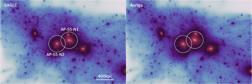
Figure 1: Present-day mass-weighted density projection of the dark matter for the AP-S5 volume in both Eagle (left) and Auriga (right). The projected rectangle has dimensions of $(3\times 2\times 3)~{}\mathrm{Mpc}$ in the $x$, $y$ and $z$ directions, respectively, centered on the centre of the mass of the two primary haloes. The white circles illustrate $\mathrm{R}_{200}$ for these two haloes. The two main haloes do not overlap in 3D space but they do in this particular $x$-$y$ 2D projection.

We focus on $\Lambda$CDM hydrodynamical simulations of two Local Group-like volumes. Each is a zoom simulation of a region of radius $2-3$ Mpc that contains a pair of large haloes with virial masses in the range $5\times 10^{11}~{}\mathrm{\mathrm{M}_{\odot}}$ to $2.5\times 10^{12}~{}\mathrm{\mathrm{M}_{\odot}}$. We refer to the four haloes, split across two volumes, as AP-$XX$-N$Y$, where $XX=$S$5$, V$1$ specifies which of the two volumes the halo is in, and $Y=1,2$ identifies the two primary haloes. AP-V$1$ and AP-S$5$ correspond to AP-$1$ and AP-$11$ in the original APOSTLE simulations described in Sawala et al. (2016) and Fattahi et al. (2016). The volumes were selected to match some of the dynamical constraints of the Local Group. The two primary haloes are required to have present-day physical separations of $\approx 800~{}\mathrm{kpc}$ and radial velocities in the range $(0-250)~{}\mathrm{km~{}s^{-1}}$. The volumes are also required to have no additional haloes of mass equal to, or greater than, the least massive of the pair within a radius $2.5~{}\mathrm{Mpc}$ of the pair midpoint. More details about the selection criteria may be found in Fattahi et al. (2016).

The ‘zoom-in’ initial conditions (ICs) were created using second-order Lagrangian perturbation theory implemented within ic_gen (Jenkins, 2010). These ICs have initial gas (dark matter) particle masses of $1.2(5.9)\times 10^{5}~{}\mathrm{\mathrm{M}_{\odot}}$, and maximum softening lengths of $307~{}\mathrm{pc}$. This resolution level corresponds exactly to the L2 resolution in Sawala et al. (2016) and Fattahi et al. (2016), and is similar to the level 4 resolution in Grand et al. (2017).

AP-$XX$-$YY$-Ea are the Eagle simulations which were run using a highly modified version of the gadget-3 code (Springel, 2005). The fluid properties are calculated with the particle-based smoothed particle hydrodynamics (SPH) technique (Lucy, 1977; Gingold & Monaghan, 1977). The Eagle  simulations adopted a pressure-entropy formulation of SPH (Hopkins, 2013), with artificial viscosity and conduction switches (Price, 2008; Cullen & Dehnen, 2010) which, when combined, are known as ANARCHY (Schaye et al., 2015).

The Auriga simulations, AP-$XX$-$YY$-Au, were performed with the magnetohydrodynamics code arepo (Springel, 2010). The gas is followed in an unstructured mesh constructed from a Voronoi tessellation of a set of mesh-generating points which then allow a finite-volume discretisation of the magneto-hydrodynamic equations. The mesh generating points can move with the fluid flow. This moving mesh property reduces the flux between cells, thus reducing the advection errors that afflict fixed mesh codes. For a detailed description we refer the reader to Springel (2010) and Grand et al. (2017).

The Auriga simulations follow the amplification of cosmic magnetic fields from a minute primordial seed field. The magnetic fields are dynamically coupled to the gas through magnetic pressure. Pillepich et al. (2017) demonstrates that the stellar mass to halo mass (SMHM) relation is sensitive to the inclusion of magnetic fields, particularly for haloes of $M_{200}\geq 10^{12}~{}\mathrm{\mathrm{M}_{\odot}}$. However, this is not important in this work as both galaxy formation models are calibrated to reproduce realistic $L^{\star}$ galaxies.

While the general method of calculating the physical fluid properties in the two simulations is different, there are some similarities. Both numerical schemes have the property that resolution follows mass, namely, high-density regions are resolved with more cells or particles. Also, both Eagle and Auriga have the same method for calculating gravitational forces: a standard TreePM method (Springel, 2005). This is a hybrid technique that uses a Fast Fourier Transform method for long-range forces, and a hierarchical octree algorithm for short-range forces, both with adaptive timestepping.

The initial conditions are chosen to produce present-day Milky Way (MW) and M31 analogues. As both the Auriga and Eagle simulations share exactly the same initial conditions, we expect several properties of the simulations to be similar. Specifically, the dark matter properties should be consistent in both simulations. Furthermore, as both simulations tune the subgrid models to recover real galaxy properties, we expect some stellar properties to be similar, but less so than the dark matter properties.

Dark matter haloes are identified using a Friends-of-Friends (FoF) algorithm (Davis et al., 1985). The constituent self-bound substructures (subhaloes) within a FoF group are identified using the SUBFIND algorithm applied to both dark matter and baryonic particles (Springel et al., 2001; Dolag et al., 2009).

Table 1 lists properties of the two primary haloes in both volumes. We see that the baryonic properties of the four haloes in the two simulations differ somewhat, with up to a factor of two difference in the stellar mass. We also tabulate the baryon fraction, $f_{\mathrm{b}}$, in each halo, which we define as the ratio of baryonic to total mass normalised by the mean cosmic baryon fraction, $\Omega_{\rm b}/\Omega_{\rm m}\sim 0.167$, within $\mathrm{R}_{200}$. We find that the baryon fraction in the Eagle simulations is systematically lower than in their Auriga counterparts. The virial properties of the haloes are all consistent, however, with small differences in virial mass and radius which are due to the different halo baryon fractions.

Fig. 1 shows a dark matter projection of the AP-S$5$ volume in both Eagle and Auriga. A visual inspection shows that the dark matter distribution of the two haloes, and their local environment, are almost identical in the two simulations. There is some variation in the location of satellite galaxies and nearby dwarf galaxies; this is likely due to the different baryonic properties and the stochastic nature of N-body simulations.

In Fig. 2 we plot the SMHM relation for the four primary haloes in the two simulation volumes, Eagle and Auriga, alongside the inferred relation from abundance matching (Behroozi et al., 2013). We also include several resolved lower mass field ‘central’ haloes from both Eagle and Auriga to give an indication of the SMHM over a broader mass range. We define the stellar masses as the total stellar mass within an aperture of $30~{}\mathrm{kpc}$. The stellar masses of the Auriga galaxies are consistently larger than those of the Eagle galaxies, at a given halo mass, over the entire range of halo masses. As both Eagle and Auriga model the same volume, the differences are not due to sample variance.

We also briefly analyse the stellar surface density profiles of the four primary haloes at the present day. We fit the surface density profiles with a combination of an exponential profile of scale radius, $R_{\rm{D}}$, and a Sersic profile of the form $\exp(R/R_{\rm{eff}})^{n}$ (Sérsic, 1963). The values of the best-fit parameters, $R_{\rm{D}}$, $R_{\rm{eff}}$ and $n$, are given in Table 1. The fit parameters of the models are consistent with the isolated MW-mass galaxies, the original Auriga haloes, presented in Grand et al. (2017). Furthermore, the stellar surface density at the solar radius is a few times $\sim 10~{}\mathrm{\mathrm{M}_{\odot}~{}pc^{-2}}$ in all of the haloes which is consistent with estimates for the Milky Way (Flynn et al., 2006). The surface density profiles, and best fit models, can be seen in Fig. 18. The galaxy stellar surface density profiles are similar in most cases in the two simulations, albeit with a systematically higher surface density in the case of Auriga.

We also calculate the $\kappa_{\mathrm{rot}}$ rotation parameter for each galaxy, a measure of the fraction of kinetic energy in organized rotation, which correlates with morphology (Sales et al., 2012). The quantity $\kappa_{\mathrm{rot}}$ is defined such that $\kappa_{\mathrm{rot}}\approx 1$ for discs with perfect circular motions and $\kappa_{\mathrm{rot}}\approx 1/3$ for systems with an isotropic velocity dispersion. Thus, a large $\kappa_{\mathrm{rot}}$ indicates a disc galaxy, whereas a lower value indicates an elliptical galaxy. $\kappa_{\mathrm{rot}}$ requires a definition of the z-axis which we take to be the direction of the total angular momentum of all stars within $30~{}\mathrm{kpc}$ of the centre of the galaxy. The large values of $\kappa_{\mathrm{rot}}$ in Table 1 are consistent with a visual inspection of Fig. 3, which shows face-on and edge-on stellar projections of the four primary haloes. In Fig. 3 we see that most of the galaxies appear to be ‘disky’ in projection, with the exception of AP-V$1$-N$2$-Ea, which has a low $\kappa_{\mathrm{rot}}$.

In general, the Auriga simulations exhibit more recognisable morphological features, spiral arms and distinct bar components (AP-S$5$-N$2$, AP-V$1$-N$1$ and AP-V$1$-N$2$). The Eagle simulations produce smoother looking discs, with little morphological evidence of either a bar or spiral arms. It is unclear what causes these morphological differences, but they could be due to different effective spatial resolutions in the two simulations. In SPH simulations, the smoothing length determines the spatial resolution, and the ratio of the smoothing length to the mean inter-particle separation is usually a free parameter taken to be $\sim 1.3$ (Price, 2012). Whereas in moving mesh simulations, the cells have a spatial radius of approximately $\sim 0.5$ the mean cell separation. Thus moving mesh simulations typically have a $\sim 1.3/0.5\sim 2.4$ times better spatial resolution at the same mass resolution.

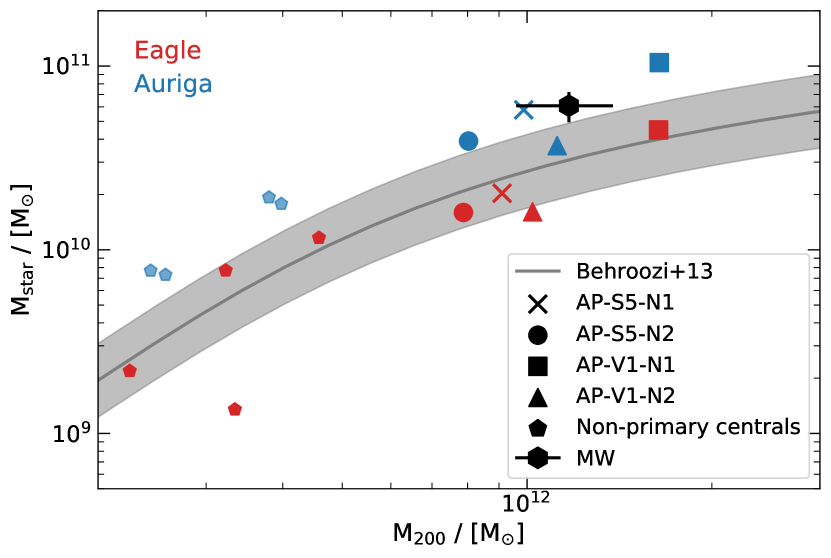
Figure 2: The stellar-mass-to-halo-mass relation in the Eagle  (red) and Auriga (blue) simulations. The four different symbols (cross, circle, square and triangle) differentiate the four different primary haloes. The smaller blue and red pentagons show the SMHM relation for ‘central’ field galaxies in the Eagle and Auriga simulations respectively. The black solid line and grey shaded region are the results of Behroozi et al. (2013) with an estimated scatter of $\pm 0.2~{}\mathrm{dex}$. We also show as a black hexagon with errorbars the estimate for the Milky Way halo mass by Callingham et al. (2019) and of the stellar mass by Licquia & Newman (2015)

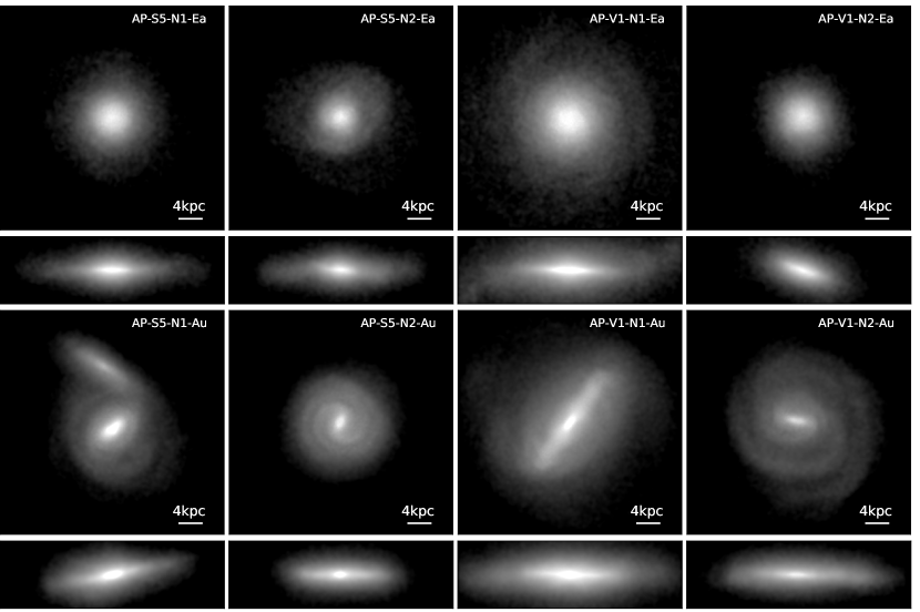
Figure 3: Mass-weighted face-on (top) and edge-on (bottom) projections of the stars in the four haloes in the Eagle and Auriga simulations at $z=0$

3 Methods and observables

3.1 Subgrid physics models

Eagle and Auriga include prescriptions for subresolution baryonic processes such as star formation (Schaye & Dalla Vecchia, 2008), metal enrichment (Wiersma et al., 2009b), black hole seeding and growth, active galactic nuclei (AGN) feedback (Springel, 2005; Booth & Schaye, 2009; Rosas-Guevara et al., 2015), radiative cooling (Wiersma et al., 2009a) and feedback from stellar evolution (Dalla Vecchia & Schaye, 2012). However, as previously noted, the implementations are rather different. In this section, we describe the qualitative differences in the SNe feedback prescriptions in the two models.

Traditionally, the energy from SN events occurring within the single stellar population (SSP) represented by a star particle is injected into a large mass of local gas (Dalla Vecchia & Schaye, 2008). If SNe energy from an SSP is injected over a mass of gas comparable to the initial stellar mass formed, the gas is heated to high temperatures, $T\geq 10^{7}~{}\mathrm{K}$. However, when the same amount of energy is distributed over a much larger mass of gas, the temperature increase experienced by the gas is much lower. This lower post-SNe gas temperature results in a shorter cooling time. When the cooling time is significantly shorter than the sound-crossing time of the gas, energy injection from SNe is unable to drive a galactic wind efficiently (e.g. Dalla Vecchia & Schaye, 2012).

In the Eagle simulations all the SNe energy from an SSP is injected in the form of thermal energy (Schaye et al., 2015). Rather than distributing the energy evenly over all of the neighbouring gas particles, the energy is injected into a small number of neighbours stochastically (Dalla Vecchia & Schaye, 2012). This method allows the energy per unit mass, which corresponds to the temperature change of a gas particle, to be defined. In these simulations each gas particle heated by SN feedback is always subject to the same temperature increase, $\Delta T_{\rm{SN}}=10^{7.5}~{}\mathrm{K}$.

The SNe feedback scheme in the Auriga simulations consists of an initially decoupled wind whose main free parameters are the energy available per unit mass of SNII and the wind velocity. The wind velocity scales with the 1-dimensional velocity dispersion of local dark matter particles. Qualitatively, SNe winds are modelled by ‘wind particles’ which are launched in an isotropic random direction carrying mass, energy, momentum and metals. Upon launch, the wind particles are decoupled from hydrodynamic forces and experience only gravity. The wind particles can recouple either when they reach a region of low-density gas (5% of the star-formation density threshold) or when they exceed a maximum travel time ($0.025$ of the Hubble time at launch). When the wind recouples, it deposits energy, momentum and metals into the gas cells it intersects.

We do not describe the AGN feedback models but detailed explanations of them can be found in Schaye et al. (2015) and Grand et al. (2017) for Eagle and Auriga, respectively. The AGN model used in the Eagle simulations in this work differs slightly from the reference model in Schaye et al. (2015). Namely, in this work the AGN model uses a viscosity which is hundred times lower than the reference model this reduces the accretion rate and growth of the black holes. This model is referred to as ‘ViscLo‘ in Crain et al. (2015). In Section 8 we discuss the possible effects of the different AGN models on our results.

3.2 Tracer particles and particle matching

The quasi-Lagrangian technique of arepo allows mass to advect between gas cells so each cell may not represent the same material over the course of the simulation. The Auriga simulations, however, include Lagrangian Monte Carlo tracer particles (Genel et al., 2013; DeFelippis et al., 2017) which enable us to track the evolutionary history of individual gas mass elements in a way that allows direct comparison to SPH gas particles in Eagle. The Monte Carlo tracer particles have been shown to reproduce the density field in various tests, including cosmological simulations, accurately (Genel et al., 2013).

In Auriga, a single tracer particle is attached to each gas cell at the beginning of the simulation. As the simulation proceeds, tracer particles can transfer across cell boundaries with a probability given by the ratio of the outward-moving mass flux across a face and the mass of the cell. This allows the tracer particles to emulate the evolution of a Lagrangian gas element. The tracer particles do not carry any physical properties. Instead, they inherit the properties of the baryonic element to which they are attached at any given time. The tracer particles introduce a Poisson noise due to their probabilistic evolution. However, as we use several million tracer particles, this noise is insignificant.

A combination of identical initial conditions and the tracer particles in Auriga allows us to perform a detailed comparison between the two simulations on the scales of individual baryonic mass-elements. In the Eagle  simulations, each dark matter particle in the initial conditions is assigned a gas particle at the start of the simulation. This represents the baryonic mass from the same Lagrangian region as the associated dark matter particle. Likewise, the dark matter particles within Auriga are assigned tracer particles. Both the tracer particles in Auriga, and the gas particles in Eagle, are assigned permanent, unique ID’s dependent on their parent dark matter particle. The unique ID assigned to each particle facilitates direct comparison of the same baryonic mass elements between the two simulations.

3.3 Ion number densities

We calculate column densities of several ionised species following Wijers et al. (2019). The total number of ions, $N_{X_{i}}$, of each species in a given mass of gas is given by,

$$N_{X_{i}}=\frac{m_{X}f_{X_{i}}}{m_{Z}},$$ (1)

where $m_{X}$ is the total mass of element $X$, $f_{X_{i}}$ is the ionization fraction of the $i^{th}$ ion, $m_{Z}$ is the mass of an atom of element $X$ and $Z$ is the atomic number of the ionized element.

We calculate the ionisation fraction of each species using the lookup tables of Hummels et al. (2017). These are computed under the assumption of collisional ionisation equilibrium (CIE). They only consider radiation from the metagalactic UV background according to the model of Haardt & Madau (2012) in which the radiation field is only a function of redshift. The lookup tables are generated from a series of single-zone simulations with the photoionisation code, cloudy (Ferland et al., 2013) and the method used for the “grackle” chemistry and cooling library (Smith et al., 2016). The ion fractions are tabulated as a function of log temperature, log atomic hydrogen number density and redshift.

In both Eagle and Auriga the masses of some elements are tracked within the code; these are hydrogen, helium, carbon, nitrogen, oxygen, neon, magnesium, silicon and iron. We calculate the number of species of each element from Eq. 1 with the total mass of each element as tracked by the code, and the calculated mass fraction of each species state. We can then make 2-dimensional column density maps of each species by smoothing the contribution from each gas particle onto a 2D grid with a two-dimensional SPH smoothing kernel. We make these 2D maps by projecting through each of the $x$, $y$ and $z$ axis. We then separate the 2D maps, which cover a region of $(8\times 8)~{}\mathrm{R}_{200}$, into $100$ annuli with linearly spaced radii. In each annulus, we have many lines-of-sight through the halo. We then take the column density at radius, $r$, to be the median column density calculated within the annulus that encloses the radius, $r$, for all three projected maps. We choose to use the median as it is more representative of a single random line-of-sight through a halo in the real universe. However, the mean value, which is often significantly higher, is also of interest as observed values can be biased by the detection thresholds of instruments.

Eagle and Auriga use different yield tables when calculating the fraction of different elements returned from SNIa to the ISM. These yield tables typically differ by $<20\%$ for the species considered in this work. However, these difference are negligible in the results presented in Section 7.1, which span many orders of magnitude. It is possible to normalise these yield fractions in post-processing, but we choose to use the simulation tracked quantities are they are self-consistent with the gas cooling.

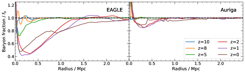
Figure 4: The baryon fraction within a sphere centred around the primary halo, AP-S$5$-N$1$, as a function of the sphere radius. The baryon fraction is calculated within $100$ spheres with a linearly increasing radius in the range $0-2.5~{}\mathrm{Mpc}$ (comoving). We repeat the process at six redshifts, $z=0,~{}1,~{}2,~{}5,~{}8$ and $10$, which are shown by the brown, purple, red, green, orange and blue solid lines, respectively. The left panel shows the results in Eagle and the right panel in Auriga. The baryon fraction is normalised by the mean baryonic-to-dark matter ratio, $f_{b}$, in the universe. The dashed black line indicates a baryonically closed system.

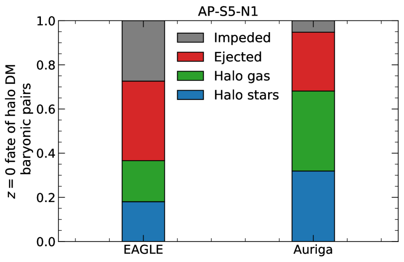
Figure 5: The present-day fate of the baryonic counterparts of the dark matter particles within $\mathrm{R}_{200}$ of the primary halo AP-S$5$-N$1$ in Eagle and Auriga. The halo stars, halo gas, ejected gas and impeded gas are shown by blue, green, red and grey bars, respectively. See the text for a detailed description of these categories.

3.4 The dispersion measure

Fast radio bursts (FRBs) are bright pulses of radio emission with periods of order milliseconds, typically originating from extragalactic sources (see review by Cordes & Chatterjee, 2019). The first FRB, which was reported by Lorimer et al. (2007), was found in archival data from the $64~{}\mathrm{m}$ Parkes radio telescope. By 2019, there were over 80 distinct FRB sources reported in the literature (see review by Petroff, 2017). In the next few years, these FRB catalogues will grow by orders of magnitude with current and future surveys detecting thousands of events per year (Connor et al., 2016).

As radiation from an FRB propagates through the intervening gas, the free electrons in the gas retard the radiation. As the retardation of the radiation is frequency dependent, this process disperses the FRB pulse, thus producing a measurable time delay between the highest and lowest radio frequencies of the pulse. The dispersion measure quantifies this time delay. The dispersion measure, from observations of the photon arrival time as a function of frequency, is given by,

$$\int(1+z)~{}n_{e}~{}dr~{},$$ (2)

which provides an integral constraint on the free electron density, $n_{e}$, along the line-of-sight from the observer to the source, where $dr$ is the path length in comoving coordinates. The free electron density and the radiation path in Eq. 2 are also in comoving units. The dispersion measure will include contributions from free electrons in the IGM (Zheng et al., 2014; Shull & Danforth, 2018), our galaxy, the Local Group, the galaxy hosting the FRB and baryons residing in other galactic haloes which intersect the sightline (McQuinn, 2014). As such, FRBs provide a possible way to investigate the presence of baryons that are difficult to observe with other methods.

In hydrodynamical simulations, we can calculate contributions to the dispersion measure from both the ISM and the hot halo of MW-like galaxies, and investigate the model dependence. The electron column density can be calculated for sightlines in a similar way to that described in Section 7.1 below. We calculate the number of free electrons for each gaseous particle or cell in the simulations by computing the number density of H ii, He ii and He iii, which dominate the total electron density; these calculations again utilise the ion fraction lookup tables of Hummels et al. (2017).

4 Baryon evolution

As we have shown in Section 2, Eagle and Auriga produce galaxies in MW-mass haloes that have roughly similar morphologies, stellar masses and stellar mass distributions. However, as the simulations are calibrated to reproduce a number of stellar properties of the observed galaxy population, these similarities are not too surprising. In this section we explore the effects of the two different hydrodynamical schemes and feedback implementations on the untuned baryon properties. In particular, we investigate the baryon fraction around the two pairs of MW and M31 analogues and how this evolves with both radius and time.

In Fig. 4 we investigate the baryon fraction within a sphere centred on the main progenitors of the AP-S$5$-N$1$ simulations, as a function of radius at six different redshifts. Even though both simulations follow the assembly of the same dark matter halo, the baryon fraction within a sphere of radius $\approx 500~{}\mathrm{kpc}$ (comoving) begins to differ significantly between $z=8$ and $z=5$. By $z=2$ the Eagle model has developed a baryon deficiency of $\geq 10\%$ within a radius of $\geq 1~{}\mathrm{Mpc}$ (comoving), extending to $\approx 2~{}\mathrm{Mpc}$ at the present day. We refer to this is the Local Group baryon deficiency. By contrast, in the Auriga simulations the baryon fraction is within $10\%$ of unity for radii $\geq 0.5~{}\mathrm{Mpc}$ (comoving) at all redshifts. Furthermore, the minimum baryon fraction within a sphere around the primary Auriga galaxy is $\approx 80\%$, approximately twice that of its Eagle counterpart.

In Table 1 the baryon fraction of AP-V$1$-N$1$-Ea is similar ($\sim 0.85\Omega_{\rm b}/\Omega_{\rm m}$) to that of the Auriga  counterpart. However, the baryon fraction of this galaxy at $z=1$ was $\sim 0.5\Omega_{\rm b}/\Omega_{\rm m}$, almost a factor of two lower than in Auriga. Furthermore, the baryon fraction within a radius of $\sim 1~{}\mathrm{Mpc}$ is $\sim 30\%$ lower than in Auriga. Thus, even the most baryon rich halo in Eagle is still baryon poor compared to the same halo in Auriga. The differences in the baryon fraction of the haloes in the local region, out to $\sim 1~{}{\rm Mpc}$, around AP-S$5$-N$1$ are representative of the sample. Thus, while we focus on the individual halo AP-S$5$-N$1$ for illustration, the general results are valid for all haloes in our sample.

In both Eagle and Auriga the halo baryon deficiency peaks at around $z=1-2$, which is consistent with the observed peak in the star formation rate in the real universe (Madau & Dickinson, 2014). However, the amplitude, spatial extent and scale of the baryon deficiency in Eagle, compared to Auriga, is striking. This difference is particularly remarkable given that the primary galaxies are relatively similar.

AGN feedback is often thought to be the cause of low baryon fractions in MW-mass, and more massive haloes in cosmological hydrodynamical simulations (Bower et al., 2017; Nelson et al., 2018; Davies et al., 2019). Nevertheless, we see from Fig. 4 that the decrease in baryon fraction in Eagle  sets in at high redshift when the halo masses, and thus the black hole masses, are much lower. These results thus imply a different driver for the low baryon fractions at the present day.

Although the two simulations predict very different local baryon fractions, both within the halo and beyond, it is difficult to ascertain which of these models is the more realistic. In practice, it is very difficult to infer the baryon fractions of real galaxies. For external galaxies this are typically derived from X-ray emission using surface brightness maps to infer a gas density profile. These inferences also require information about the temperature and metallicity profiles, which are difficult to measure accurately with current instruments (Bregman et al., 2018).

In the Milky Way, the baryonic mass in stars, cold and mildly photoionised gas and dust is estimated to be $0.65\times 10^{11}~{}\mathrm{\mathrm{M}_{\odot}}$ (McMillan, 2011). The total mass of the halo, which is dominated by dark matter, is estimated to be $(1.17\pm 0.15)\times 10^{12}~{}\mathrm{\mathrm{M}_{\odot}}$ (Callingham et al., 2019). Assuming a universal baryon fraction of $\Omega_{\rm b}/\Omega_{\rm m}\approx 0.157$ (Planck Collaboration et al., 2013) implies that $0.8\times 10^{11}~{}\mathrm{\mathrm{M}_{\odot}}$ of the MW’s baryons are unaccounted for. There is strong evidence that some fraction of these unaccounted baryons resides in a hot gaseous corona surrounding massive haloes; however, it total mass remains uncertain. An accurate estimate of the mass of the MW hot halo requires knowledge of the gas density profile as a function of radius. While the column density distribution of electrons is constrained in the direction towards the LMC (Anderson & Bregman, 2010), there is a degeneracy between the normalisation and the slope of the electron density profile (Bregman et al., 2018). Assuming a flat density profile (e.g. Gupta et al., 2012, 2014; Faerman et al., 2017), the MW appears to be ‘baryonically closed’. However, for faster declining density profiles (see Miller & Bregman, 2015; Li & Bregman, 2017), the gaseous halo out to $\mathrm{R}_{200}$ contains only half of the unaccounted baryons. Therefore, the predictions of Fig. 4 for both Eagle and Auriga are consistent with observations given the uncertainties.

5 The missing halo baryons

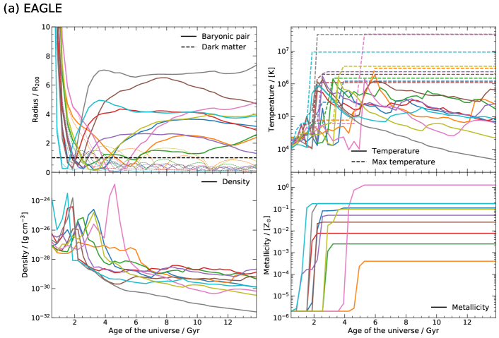
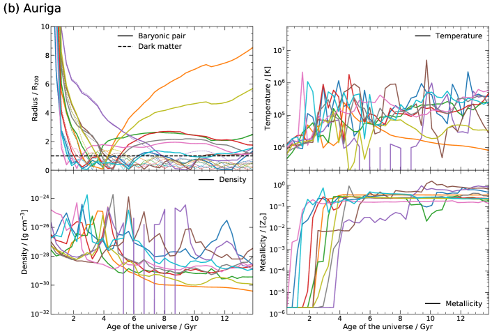
Figure 6: The evolution of 10 randomly selected halo baryonic tracer particles classified as ‘ejected’ from an (a) Eagle  and (b) Auriga halo. For both (a) and (b), the top-left, top-right, bottom-left, and bottom-right panels show the radius from halo centre, mean temperature, density and metallicity as a function of time. The particle properties are sampled at $60$ snapshots linearly spaced as a function of the age of the universe. The radius is given in units of $\mathrm{R}_{200}(z)$. The top-left panel also includes the radial position of the dark matter counterpart of each baryon particle; these are illustrated with a dashed line of the same colour. In the bottom-right panel, which shows the metallicity, there are several lines which lay on top of one another and thus are not visible. The same random particle is identified in each panel by the same coloured line.

In this section we carry out a detailed analysis, on a particle-by-particle basis, of the differences in the present-day baryon contents of the Eagle  and Auriga Local Group analogues. As we described in Section 3.2, each dark matter particle is assigned a gas particle, or a tracer particle, which shares the same Lagrangian region in the initial conditions. In the absence of baryonic physics, these particles would evolve purely under gravity and would thus end up in the same halo as their dark matter counterparts. We refer to these as ’predestined’ particles. However, hydrodynamics and feedback will significantly alter their fate.

We start our analysis by identifying all the dark matter particles present in each of the primary haloes at $z=0$. We then identify the baryonic companions of these dark matter halo particles and categorise their $z=0$ state, as illustrated in Fig. 5, classifying them into the following four categories:

• Halo gas: gas particles within $\mathrm{R}_{200}$ of the primary halo

• Halo stars: star particles within $\mathrm{R}_{200}$ of the primary halo

• Ejected gas: gas particles which are outside $\mathrm{R}_{200}$ at $z=0$ but had closest approach radii smaller than $\mathrm{R}_{200}$ at a previous redshift

• Impeded gas: gas particles which are outside $\mathrm{R}_{200}$ at $z=0$ and had closest approach radii larger than $\mathrm{R}_{200}$ at all previous redshifts.

It is important to note that Fig. 5 does not include baryons in the present-day halo if the dark matter counterpart is not in the halo. These baryons make a negligible contribution to the halo baryon mass.

There are several important differences in Fig. 5 between Eagle and Auriga. About $35\%$ of the baryonic pairs of the $z=0$ dark matter halo particles lie inside the primary halo of the Eagle simulation, whereas in the Auriga  simulations approximately $70\%$ of the baryon counterparts are within $\mathrm{R}_{200}$. The baryons that lie within the halo are split between stars and gas in a roughly $1:1$ ratio in both simulations.

While the fate of the retained baryon counterparts is similar in the two simulations, the evolution of the absent baryons is considerably different. In Eagle we find that almost half of the baryon counterparts which are missing never entered the halo, whereas in Auriga almost $\approx 90\%$ of the absent baryons entered the halo before being ejected, presumably by SNe or AGN feedback.

5.1 Ejected gas

In Fig. 6 (a) and (b) we show the evolution of 10 randomly selected ‘predestined’ halo baryons which have been classified as ‘ejected’. The particles are sampled at $60$ snapshots linearly spaced as a function of the age of the universe, corresponding to a temporal resolution of $\approx 200~{}\mathrm{Myr}$.

In both simulations we see that the radial trajectories of both the gas and paired dark matter particles are generally very similar at early times. As the dark matter and baryon counterparts get closer to the main halo, their paths deviate and there is a tendency for gas accretion to be delayed relative to dark matter.

Following accretion into the halo, the trajectory of the gas begins to differ significantly from that of the dark matter. This deviation is caused by hydrodynamical forces which determine the subsequent evolution of the baryons. Most of the baryonic particles sampled in Fig. 6 (a) and (b) reach a high density upon accretion and increase their metallicity. This behaviour is consistent with halo gas that has cooled, been accreted onto the central galaxy and later ejected.

Focusing first on Eagle, Fig. 6 (a), we see that most of the randomly selected ‘ejected’ particles were ejected over $6~{}\mathrm{Gyr}$ ago. In general, these particles reach a maximum radius, and near-constant, separation of $\approx(3-8)\mathrm{R}_{200}$ very quickly. At the present day, this corresponds to a physical distance of $\approx(500-1500)~{}\mathrm{kpc}$ and is consistent with the conclusions of Section 4 which reveals a baryon deficient Local Group on scales of up to $2~{}\mathrm{Mpc}$. There also appears to be a general trend in that the earlier the gas ejection, the greater its radial separation from the primary galaxy.

Fig. 6 (a) shows that prior to being ejected, most of the Eagle gas was cold but then underwent a sudden temperature increase, with maximum temperatures regularly exceeding $10^{7}~{}\mathrm{K}$. The ejection of the gas from the halo rapidly follows the temperature increase. This process most likely proceeds as follows: the cold gas is part of the galaxy’s ISM; some of it is heated to a temperature $T\geq 10^{7}~{}\mathrm{K}$ either directly by SNe feedback or indirectly by interaction with a SNe-heated particle. The hot gas then gains energy and is accelerated to a velocity that exceeds the escape velocity of the halo. This gas can then escape beyond $\mathrm{R}_{200}$ and join the low-density IGM where it remains until the present day. It is interesting that much of the ejected gas does not have a maximum temperature, $T=10^{7.5}~{}\mathrm{K}$. This indicates that this gas was not directly heated by SNe but rather by interactions with SNe-heated gas.

In Fig. 6 (b) we see that the evolution of both baryons and dark matter is similar in Auriga and Eagle before ejection. However, in Auriga, the ejected gas typically reaches a maximum radial distance of $\sim 3\mathrm{R}_{200}$ before turning back and falling into the halo by the present day. Thus, the ‘ejected’ gas in Auriga likely has a shorter recycling timescale than the gas in Eagle, much of which never reenters the halo. However, gas that was ejected at early times and re-accreted is not, by definition, included in Fig. 6 (b). Short recycling times in Auriga were first reported by Grand et al. (2019) who show the model gives rise to efficient galactic fountains within the inner $\sim 30~{}\mathrm{kpc}$, with median recycling times of $\sim 500~{}\mathrm{Myr}$ in MW-mass haloes.

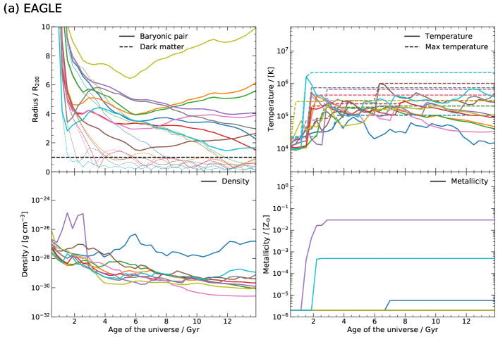
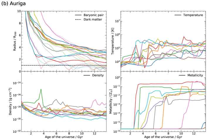
Figure 7: The evolution of 10 randomly selected halo baryonic tracer particles classified as ‘impeded’ from an (a) Eagle and (b) Auriga halo. For both (a) and (b), the top-left, top-right, bottom-left, and bottom-right panels show the radius from halo centre, temperature, density and metallicity as a function of time. The particle properties are sampled at $60$ snapshots linearly spaced as a function of the age of the universe. The radius is normalised to the (time-dependent) $\mathrm{R}_{200}$. The top-left panel also includes the radial position of the dark matter counterpart of each baryon particle; these are illustrated with a dashed line of the same colour. In the bottom-right panel, which shows the metallicity, there are several lines which lay on top of one another and thus are not visible. As with Fig. 6 the same random particle is identified in each panel by the same coloured line.

5.2 Impeded gas

We now analyse the evolution of ten randomly selected ‘predestined’, baryonic particles which have never entered the primary halo. These are plotted in Fig. 7 (a) and (b) for Eagle and Auriga, respectively. In Fig. 7(a) we see that about half the randomly-selected particles in Eagle make their initial approach at redshift, $z\sim 2-3$. As the dark matter particles are accreted into the halo, their baryon counterparts start being impeded at a radius $\sim 4\mathrm{R}_{200}$. The subsequent fate of these particles can differ substantially. About half of them remain at a distance $\geq 3\mathrm{R}_{200}$ until the present day, whereas the other half continue to approach the primary halo and are almost accreted by $z=0$.

The (maximum) temperature of the ‘predestined’ impeded particles in Eagle is shown in the top-right panel of Fig. 7 (a). The overall temperature evolution of all impeded particles is quantitatively similar. Initially, the gas is at low temperature, $\approx 10^{4}~{}\mathrm{K}$, but as it approaches the halo, it is subject to an almost instantaneous temperature rise to $\approx 10^{6}~{}\mathrm{K}$. Since the maximum temperature of the gas is always well below $10^{7.5}~{}\mathrm{K}$, this rise is not the result of direct SNe or AGN heating. Furthermore, before closest approach, these gas particles also have low density and metallicity, with one or two exceptions. These properties are consistent with pristine gas within the IGM, thus confirming that direct feedback did not heat these particles.

In Fig. 7 (b) we see that the accretion time of the dark matter counterparts of the ten randomly selected impeded baryons in Auriga is recent, within the last $\approx 4~{}\mathrm{Gyr}$, for most particles. In Eagle we saw that before closest approach, the baryon particles were relatively unenriched, cold and at low density showing no sign of interaction with nearby galaxies. However, as seen in the bottom right panel of Fig. 7 (b), much of the impeded gas in Auriga is enriched; this suggests the cause of the impediment could be local interactions.

In Fig. 8 we show the mass-weighted distribution of first accretion times of all dark matter particles associated with ‘predestined’ baryon particles classified as ‘impeded’. The Eagle  simulations have a weakly bimodal distribution: the dark matter associated with impeded gas was accreted either at early or at late times. In the Auriga  simulations the late accreted population dominates.

The presence of hot quasi-hydrostatic haloes can impede gas accretion at late times. haloes of mass $\gtrapprox 10^{12}~{}\mathrm{\mathrm{M}_{\odot}}$ have massive hot gaseous coronae. These gaseous haloes, which often extend beyond $\mathrm{R}_{200}$, can exert pressure on the accreting gas and thus delay its accretion. The accretion of the collisionless dark matter is, of course, not impeded. The process impeding gas accretion at early times and late time in Eagle is likely to be similar. However, the progenitors of the present-day primary haloes are not massive enough at high redshift to support massive atmospheres of primordial gas to explain the observed scale of suppressed accretion so most of the gaseous atmosphere must be gas that was reheated and ejected.

The explanation is provided in Fig. 9 which shows temperature projections of the AP-S$5$-N$1$ halo at four times between $z=3.5$ and $z=2$ in both Eagle and Auriga. We overlay the positions of sixteen randomly selected baryon/dark matter pairs chosen so that they were ‘impeded’ at early times in Eagle. The same pairs, originating from the same Lagrangian region in Auriga, are also overlaid. The blue circles show the $x,y$ positions of the dark matter and the white circles those of the baryons. The white dotted line connects the baryon/dark matter pairs to help visualise the differences in the evolution of the two species.

We see that in Eagle the MW progenitors are encased in a hot, $\approx 10^{6}~{}\mathrm{K}$, corona of gas that occupies a volume of radius twice as large as that of the Auriga counterparts. This gas halo consists of a mixture of accreting primordial gas and hot outflowing winds fuelled by feedback from the central galaxy. As shown in Fig. 6, gas particles in the ISM can be heated by SNe feedback, generating a hot, outflowing wind that can reach distances of up to $4\mathrm{R}_{200}$ in less than $1~{}\mathrm{Gyr}$. This outflowing gas interacts with the accreting gas, applying an outward force sufficient to delay or prevent accretion. This leads to large amounts of ‘predestined’ gas ‘impeded’ from accreting at early times in Eagle (as seen in Fig. 5). The overlaid particles in Fig. 9 succinctly demonstrate this process.

In contrast, the Auriga haloes have hot gaseous components that barely extend beyond $\mathrm{R}_{200}$ and do not evolve in time significantly. As the hot component in Auriga is less massive and cooler than in Eagle, the dark matter/baryon pairs evolve similarly until they reach $\sim 1.5\mathrm{R}_{200}$. At radii $\leq 1.5\mathrm{R}_{200}$ gas accretion is delayed relative to the dark matter by hydrodynamical forces. However, it appears less than $5\%$ of gas is completely prevented from accretion.

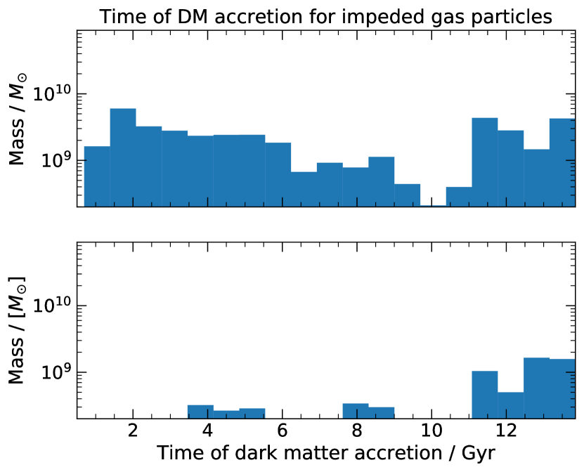
Figure 8: Mass-weighted histogram of the age of the universe at the time of accretion of the dark matter particles associated with ‘predestined’ baryon particles that have been impeded. The top panel shows results for the AP-S$5$-N$1$ halo in Eagle and the bottom panel for Auriga. This shows that cosmic gas accretion is significantly impeded at all times in Eagle, whereas Auriga only impedes cosmic gas accretion, relative to dark matter accretion, at late times.

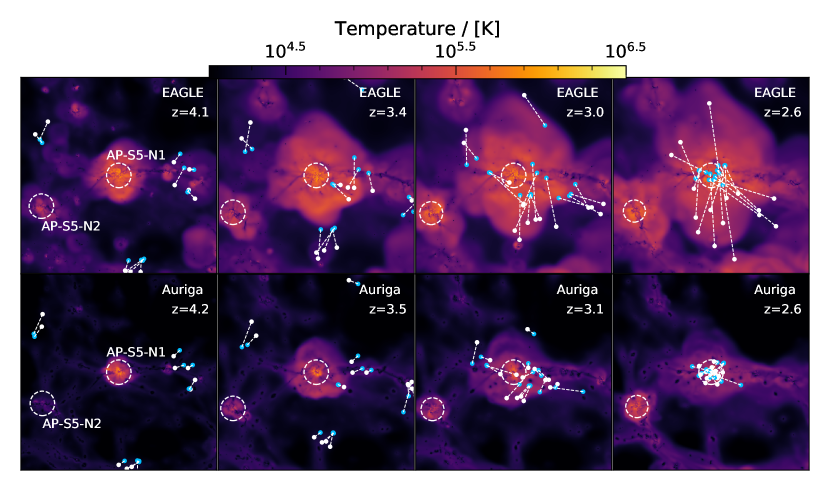
Figure 9: Mass-weighted temperature projections through a region of size $(16\times 16\times 24)~{}\mathrm{R}_{200}$ centred on the location of the progenitor of the primary galaxy in AP-S$5$-N$1$ at four redshifts, $z\sim 4,3.5,3,2.5$. Results are shown for both Eagle (top row) and Auriga (bottom row). The white and blue circles show the positions of sixteen randomly selected baryon-dark matter counterparts which are ‘impeded’ at early times in Eagle. The same counterparts, originating from the same Lagrangian region, are shown in Auriga. The white dotted lines connect the baryon/dark matter counterparts. The white dashed circles identifies the $\mathrm{R}_{200}$ of the two main haloes.

5.3 The fate of impeded and ejected baryons

Fig. 10 shows the projected dark matter and gas density of both ‘ejected’ and ‘impeded’ baryons that were ‘predestined’  to end up in the primary halo but are missing. In the Eagle simulations, the present-day distribution of these missing baryons is different for the ‘impeded’ and ‘ejected’ components. The impeded gas is elongated roughly along the $x$-axis which, as can be seen in the projected dark matter distribution, traces a local filament. By contrast, the ejected gas tends to be elongated along the $y$-axis, that is, perpendicular to the filament.

The impeded gas flows to the halo along the filament and would have been accreted by the halo had the pressure of the hot halo not impeded it. Thus, it remains in the filament, centred around the halo. The ejected material, on the other hand, finds the path of least resistance, which is perpendicular to the filament: along the filament direction the wind encounters relatively high density gas while in the perpendicular direction, the density and pressure of the surrounding medium drop rapidly. As a result, gas ejected perpendicular to the filament can reach larger radii, giving rise to the elongated distribution seen in Fig. 10.

An interesting detail in Fig. 10 is the transfer of baryons between the M31 and MW analogues. This is due primarily to the effect of gas ejection from both galaxies which can cause cross-contamination. This process is an example of halo gas transfer, (see Borrow et al., 2020) and indicates that the proximity of M31 may have influenced the evolution of the MW, although the amounts of gas transferred are very small.

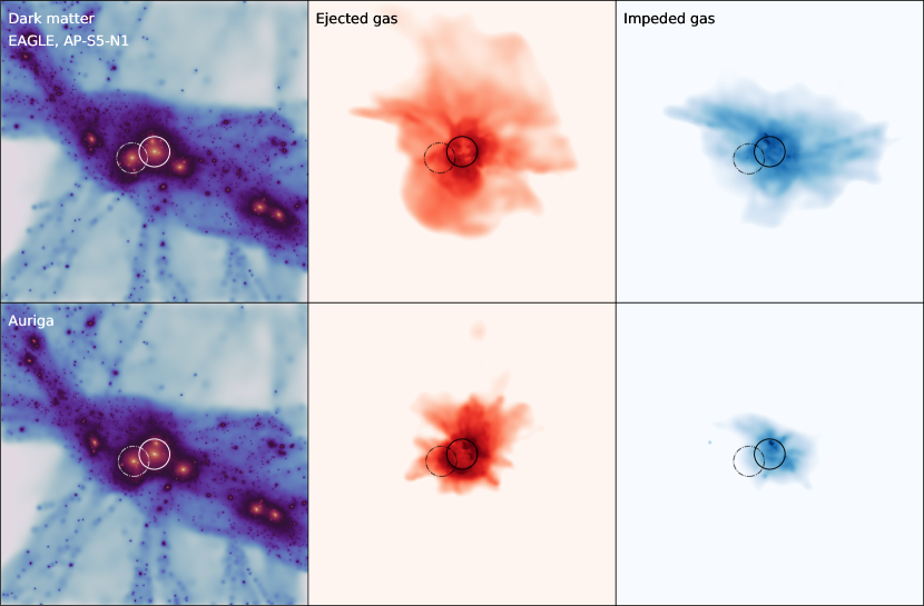
Figure 10: The $z=0$ projected density of dark matter (left), ejected baryons (center) and impeded baryons (right) for the AP-S$5$-N$1$ halo in both Eagle (top) and Auriga  (bottom). The projected cuboid has dimensions of $20\times 20\times 8~{}\mathrm{\mathrm{R}_{200}}$ in the $x$, $y$ and $z$ directions, respectively. The solid white/black circles indicate $\mathrm{R}_{200}$ of the halo AP-S$5$-N$1$ and the dashed-dotted circles that of AP-S$5$-N$2$.

While the two simulations predict very different morphologies for the ejected baryons, these differences are likely undetectable in the real universe because of the low density of ejected material.

6 Understanding the differences

In Fig. 11 we show histograms of the gas density and temperature weighted by mass, metal mass and radial velocity for both Eagle and Auriga at four redshifts. All gas particles/cells within a sphere of radius $3~{}\mathrm{R}_{200}$ around the centre of the primary halo of AP-S$5$-N$1$ are included. As in Section 4, we focus on this particular example but our general results are valid for all haloes in our sample.

We can see in the figure the gas responsible for impeding accretion in Eagle  at $z=2-3$: it is hot, $\geq 10^{6}~{}\mathrm{K}$, low density, $\sim 10^{-4}~{}\mathrm{cm^{-3}}$, slightly metal-enriched and outflowing with a mean radial velocity exceeding $100~{}\mathrm{km~{}s^{-1}}$ relative to the centre of mass of the halo. This gas component is visible from $z=3$ until $z=1$. In Auriga gas with similar temperature and density is less enriched and is not outflowing. There is some hot enriched gas with large outflow velocities at all redshift, but this gas appears to cool and mix with inflowing material as there is no evidence of less dense and slightly cooler outflows.

At higher redshift, the majority of the metals in Fig. 11(b) reside in hot, diffuse gas. As shown by Fig. 11 (c) this material is outflowing. Interestingly, we do not see any evidence of a significant cooler metal component developing until about $z=1-2$. When this cooler metal component appears, it is radially inflowing, suggesting the recycling of earlier outflows.

In Auriga we first see a population of metal-enriched gas that is both hot and dense at approximately $z=3$. By $z=2$, this enriched gas appears to have cooled and increased in density. This is inferred from distribution of metals. These features suggest the presence of galactic fountains even at high-redshift. The Auriga haloes also contain a component of very dense gas, $n_{\rm H}\geq 10^{-2}~{}\mathrm{cm^{-3}}$, with temperature ranging between $T\approx 10^{4}-10^{7}~{}\mathrm{K}$. This is a further indication of efficient galactic fountains: the high densities lead to short cooling times, of order $\sim 200~{}\mathrm{Myr}$, and, for this substantial amount of gas to be present, it must be continuously replenished by the heating of dense gas by feedback.

The differences in the nature of outflows in Eagle and Auriga could be due to differences in the SNe subgrid models. The Eagle SNe feedback model specifies the temperature increase of gas particles. In this model, SNe energy is effectively saved up and released in concentrated form stochastically. This technique means that gas is heated to higher temperatures less frequently, thus preventing the over-cooling problem (Dalla Vecchia & Schaye, 2012). Whereas in Auriga, the energy injected per unit mass of SNII is fixed. This difference in the model causes gas in Eagle to reach higher temperatures post-SNe feedback.

The total cooling efficiency of moderately enriched gas has a local minimum around a temperature of $10^{7}~{}\mathrm{K}$ and increases quite steeply both with increasing and decreasing temperature (see e.g. Fig. 9 of Baugh, 2006). Thus, a post-feedback temperature lower than $10^{7}~{}\mathrm{K}$ leads to both a higher cooling rate and lower thermal energy. When these effects are combined, the cooling time can be reduced by an order of magnitude or more. The lower post-feedback temperature in Auriga could allow SNe-heated gas to radiate a significant fraction of the injected energy on a timescale of order several hundred million years. This reduced cooling time would facilitate short recycling times for gas in Auriga and prevent the build up of a hot, SNe-fueled atmosphere at high redshift.

In Eagle, by contrast, feedback heats the gas to $10^{7.5}~{}\mathrm{K}$, and thus radiative cooling is relatively inefficient. Figure 8 of Kelly et al. (2020) shows the density and temperature of gas particles $500~{}\mathrm{Myr}$ before and after SNe heating in the Eagle reference simulation. That figure shows that gas particles that experience SNe feedback decrease their density by over two orders of magnitude within $\leq 20~{}\mathrm{Myr}$ of being heated. This expansion prevents efficient radiative cooling and also makes the gas buoyant so that it is accelerated out through the halo (Bower et al., 2016).

Fig. 12 shows a mass-weighted projection of the radial velocity of the gas in AP-S$5$-N$1$ for both Eagle (top row) and Auriga  (bottom row) at five redshifts, $z\sim 0,~{}1,~{}2,~{}3,~{}4$. It is clear from these projections that rapid outflowing material extends well beyond the halo, reaching distances of $\sim 4\mathrm{R}_{200}$ at $z=4$ in Eagle. These strong, halo-wide outflows are readily visible until $z=1$. By contrast, in Auriga   the mass-weighted radial velocity of the outflows is much slower, and their spatial extent is smaller. These radial velocity projections indicate that Eagle haloes experience strong outflows with high covering fractions. A high outflow velocity, combined with a large covering fraction, can impede cosmological gas accretion on the scale of the entire halo. By contrast, in Auriga   we see less extended outflows because a significant fraction of the SNe-heated material cools and is efficiently recycled near the centre of the halo. van de Voort et al. (2021) shows that the magnetic fields, included in the Auriga  simulations, can reduce the outflow velocities of gas around the central galaxies. This extra pressure from magnetic fields in Auriga could be contributing to the reduced gas ejection from the halo compared to that found in Eagle.

Another factor that can vary the velocity and spatial extent of outflows is the potential depth. In Fig. 13 we show the approximate circular velocity profiles as a function of radius in the four primary haloes in both Eagle and Auriga at $z=0$. These approximate circular velocity profiles are calculated from the total enclosed mass assuming spherical symmetry. We see that in the inner $50~{}\mathrm{kpc}$ the circular velocity is systematically higher in Auriga, by up to as much as $\sim 100~{}\mathrm{kms}^{-1}$. This difference is because the Eagle model is much more efficient at driving winds from the central galaxy, propagating out to scales exceeding the virial radius (Mitchell et al., 2020a). This process reduces the density in the inner region, thus reducing the escape velocity and making future gas ejection more efficient. Whereas in Auriga the opposite happens, as wind is inefficient at removing gas from the central region, the central density increases, thus deepening the potential well.

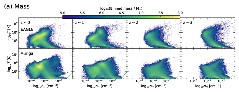
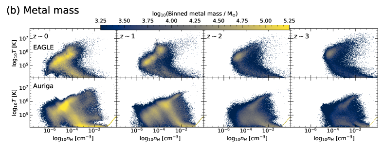
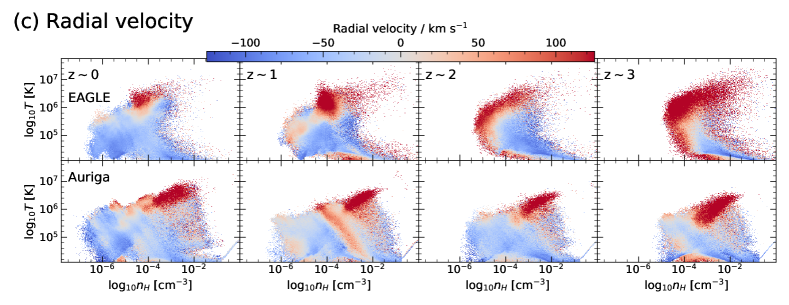
Figure 11: Gas density-temperature diagrams for a primary halo, AP-S$5$-N$1$, in both Eagle (top row) and Auriga (bottom row). The histograms are coloured according to (a) mass, (b) metal mass and (c) mass-weighted radial velocity. They include all gas with temperature $T>10^{4}~{}\mathrm{K}$ that is within radius, $r<3\mathrm{R}_{200}$, of the primary halo. The four columns show the gas distributions at four redshifts, $z\sim 0,~{}1,~{}2,~{}3$, from left to right, respectively. The histograms are generated with $300$ logarithmically spaced bins in the density range, $10^{-8}-1~{}\mathrm{cm^{-3}}$, and temperature range, $10^{3.5}-10^{7.5}~{}\mathrm{K}$.

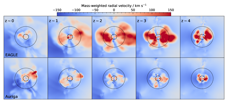
Figure 12: Mass-weighted projection of the radial gas velocity for AP-S$5$-N$1$ in both Eagle (top row) and Auriga (bottom row) at five redshifts, $z\sim 0,~{}1,~{}2,~{}3,~{}4$, from left to right, respectively. The region of these projections has size $(16\times 16\times 2)~{}\mathrm{R}_{200}$ in the $x$, $y$ and $z$ directions, respectively, where the $z$-axis is into the page. The solid black circle indicates $\mathrm{R}_{200}$ and the dashed back curve $4\times\mathrm{R}_{200}$.

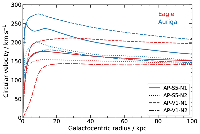
Figure 13: The approximate circular velocity of the four primary haloes in both Eagle and Auriga at $z=0$. The circular velocity, $V_{\rm circ}$, at radius $r$ is calculated from the total enclosed mass, $M(<r)$, assuming spherical symmetry $V_{\rm circ}^{2}=GM(<r)/r$ where $G$ is the gravitational constant. The Eagle and Auriga simulations are shown in red and blue, respectively.

As described in Section 2, the gas dynamics in Auriga are followed with a moving-mesh technique. Several studies have investigated the differences between moving-mesh and particle-based hydrodynamics techniques in the context of galaxy formation simulations (Sijacki et al., 2012; Kereš et al., 2012; Vogelsberger et al., 2012; Torrey et al., 2012; Bird et al., 2013; Nelson et al., 2013). A general result from these studies is that gas in moving-mesh simulations cools more efficiently than in their particle-based counterparts. The cooling efficiency of hot gas is artificially suppressed in particle-based simulations by spurious viscous heating and the viscous damping of SPH noise on small scales. Furthermore, moving-mesh simulations model energy dissipation more realistically by allowing cascading to smaller spatial scales and higher densities (Nelson et al., 2013). As we mentioned earlier, we expect these difference to be subdominant to the large differences in the subgrid models between Eagle and Auriga.

7 Observational tests

We have shown in Sections 4 and 5 that the Eagle and Auriga simulations predict very different baryon cycles around our MW and M31 analogues. We now turn to the observable signatures of strong outflows in Eagle and galactic fountains in Auriga. We present mock observations of absorber column densities and dispersion measure around our MW and M31 analogues. We aim to construct mappings between the physical state of the baryons and real observables and, in particular, to identify observables that may be sensitive to the differences in the gas properties seen in the Eagle and Auriga simulations.

7.1 Column densities

We show, in Fig. 14, the regions of the density-temperature plane where different species are relatively abundant. The contours enclose regions where each species contributes $10$ per cent of the maximum ion fraction of the respective element in collisional ionisation equilibrium at $z=1$. We show these contours as they highlight regions of the density-temperature phase space where each species is likely to be detected. This analysis is similar to Wijers et al. (2020) which analysed lower resolution, large volume cosmological simulations using the Eagle galaxy formation model.

The species that probe the hottest gas, at $T\geq 10^{6}~{}\mathrm{K}$, are typically O vii   O viii and Mg x. However, there is a degeneracy as these ionisation states are also plentiful in lower temperature, lower density gas. In the absence of other observables, it is difficult to distinguish whether detection of these ions is from a low density or a high density region. However, given that, in practice, the detection of these lines requires a moderately high column density, it is likely that any detection will be from gas at high density and, thus, high temperature. We also see in the figure that Ne vi, Ne viii and O vi probe a cooler component, at $T\leq 10^{6}~{}\mathrm{K}$. This transition temperature, $T=10^{6}~{}\mathrm{K}$, is a significant threshold as it has the potential to distinguish hydrostatic gas at the virial temperature of MW-mass haloes from hotter gas heated by feedback energy.

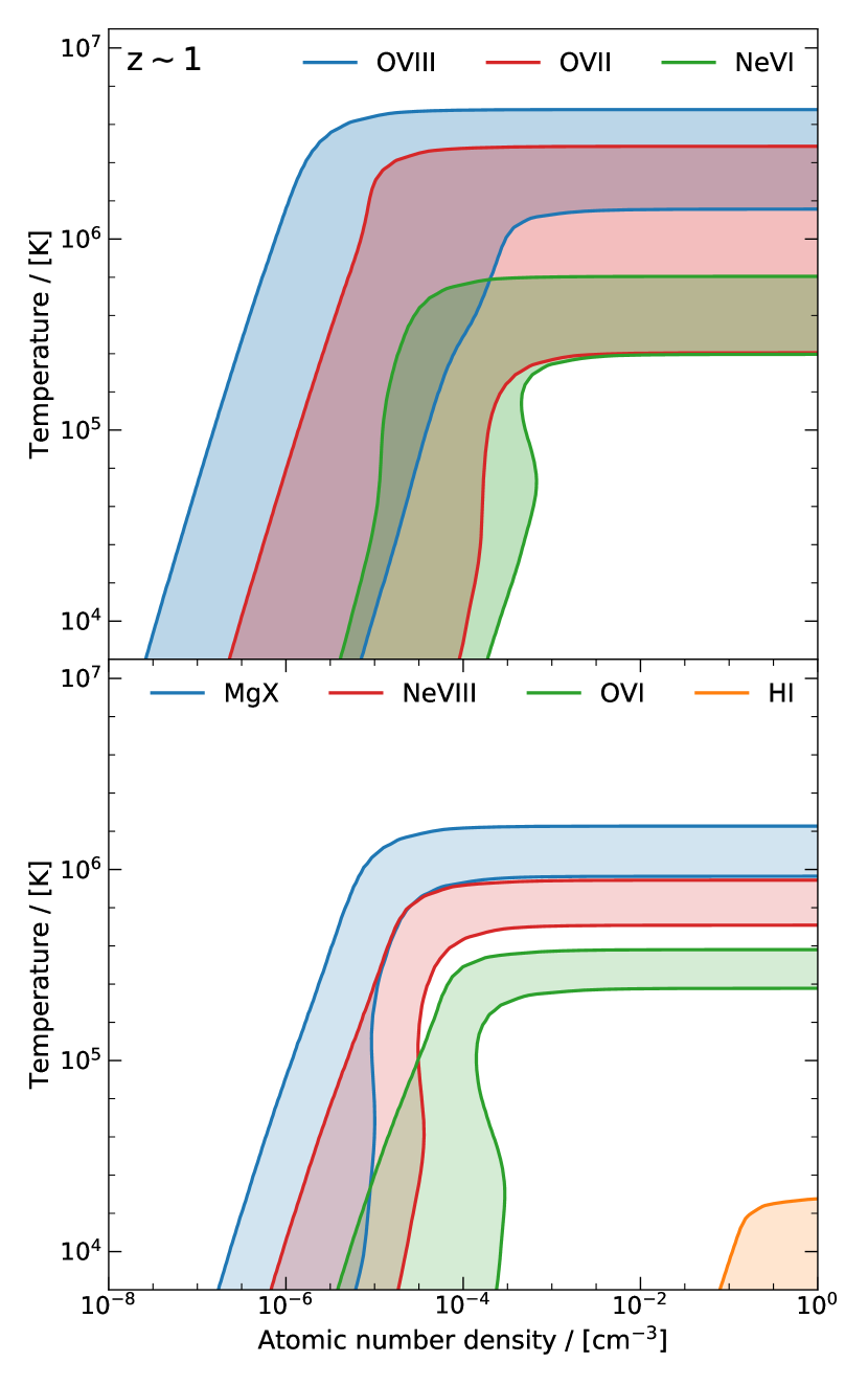
Figure 14: Temperatures and densities at which different metal species occur at $z=1$. The ion fractions are calculated from the lookup tables of Hummels et al. (2017), assuming only radiation from the metagalactic UV background according to the model of Haardt & Madau (2012). These lookup tables are computed under the assumption of collisional ionisation equilibrium (CIE). The contours for each of the indicated species are at 10 per cent of the maximum ion fraction. The top panel shows Ne vi (green), O vii (red) and O viii (blue) and the bottom panel H i (orange), O vi (green), Ne viii (red) and Mg x (blue).

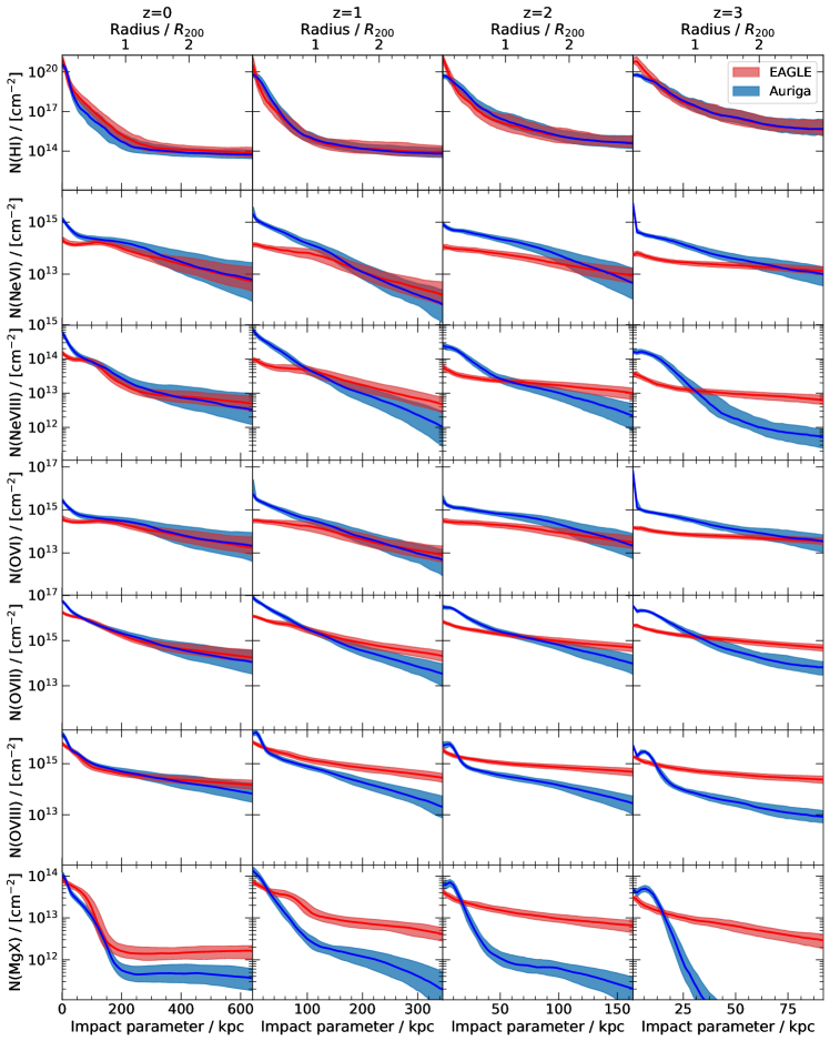
Figure 15: Atomic column number densities of several species as a function of impact parameter from the centre of the primary halo in both the Eagle (red) and Auriga (blue) simulations, out to $3\mathrm{R}_{200}$ at four redshifts $z\sim 0,~{}1,~{}2,~{}3$ from left to right, respectively. From top to bottom, the rows show results for H i, Ne vi, Ne viii, O vi, O vii, O viii and Mg x, respectively. The column density at a fixed radius, $r$, for each halo is calculated by taking the median column density of many sightlines through a small annulus. We also compute the lower and upper quartiles of the column density in each annulus. The solid lines are the mean of the median column density, at each radius, for all four haloes. The shaded regions illustrate the range between the mean of the lower and upper quartiles for all of the haloes. We choose to use the median and quartiles as these are more comparable to a single random line-of-sight through a halo in the real universe.

The species O vii and O viii are well suited for identifying very hot outflows. Unfortunately, these ions are challenging to observe in the real universe because the wavelengths of their lines are so short, $\sim 20~{}\mathrm{\textup{\AA}}$. These highly ionized stages of oxygen, the most abundant metal, have transitions that are detectable in X-rays. However, even modern X-ray instruments do not have the required resolution. Ne vi, Ne viii   Mg x  and O vi probe a similar, but typically cooler component of gas, but have much longer transition wavelengths, e.g. $558~{}\mathrm{\textup{\AA}}$, $770~{}\mathrm{\textup{\AA}}$, $610~{}\mathrm{\textup{\AA}}$ and $1032~{}\mathrm{\textup{\AA}}$, respectively. These are readily detectable with UV instruments and represent good probes of hot, collisionally ionized gas, easier to detect than than their X-ray counterparts, O vii and O viii.

We now consider each of the ions considered in Fig. 15, one at a time. We begin with the column density profile of H i   shown in the top row of Fig. 15. In general, the H i column density profile is similar at all redshifts in both simulations. The profile is centrally peaked and falls off rapidly, typically decreasing by about $4$ orders of magnitude within the first $100~{}\mathrm{kpc}$, where it flattens to a near constant number density of $10^{15}~{}\mathrm{cm^{-2}}$.

Between $z=3$ and $z=1$, the mean and scatter of the H i column density at fixed impact parameter agree well in both Eagle and Auriga. However, at $z=0$, there is a slight systematic offset in Eagle where the H i column densities are about a factor of five higher than in Auriga. The offset diminishes in both the centre, $<30~{}\mathrm{kpc}$, and beyond $\mathrm{R}_{200}$. The similarity of the H i distributions in both simulations is not surprising. In particular, we see in Fig. 11 that the distribution of gas at high densities and low temperatures, where H i typically occurs, is very similar in the two (see Fig. 14).

The second, third and fourth rows from the top of Fig. 15 show the column density profiles of O vi, Ne vi and Ne viii, respectively. We discuss the distributions of these ions collectively, as they have similar general trends and typically probe gas at the same density and temperature, as demonstrated in Fig. 14. O vi, Ne vi and Ne viii probe progressively hotter populations of dense gas, increasing from $10^{5.5}~{}\mathrm{K}$ up to $10^{6}~{}\mathrm{K}$. Ne vi typically probes a broader range of temperatures, $\sim 0.4~{}\mathrm{dex}$, compared to $\sim 0.2~{}\mathrm{dex}$ for O vi and Ne viii.

At $z=0$, the column densities of O vi, Ne vi and Ne viii in Auriga are higher than in Eagle at all radii, but the difference is maximal at the centre of the halo. Outside the central region, beyond $\sim 30~{}\mathrm{kpc}$, the differences in column density are fairly small, typically a factor of two or less. Although the mean column density differs at a given impact parameter, the range of column densities for the whole sample typically overlaps. The differences, however, can be substantial at higher redshift, $z\geq 1$. In Fig. 15 we see a general behaviour in the O vi, Ne vi and Ne viii profiles in both Eagle and Auriga. In Eagle, the column density distributions are relatively flat, typically decreasing by only an order of magnitude over a radial range $3\mathrm{R}_{200}$. In contrast, in Auriga, the central column densities are typically higher and decrease much faster, dropping by over four orders of magnitude over the same radial range.

The differences in the column density profiles of O vi, Ne vi and Ne viii at $z\geq 1$ in Eagle and Auriga are most notable in both the innermost and outermost regions. In Auriga, the column densities of these ions are higher in the centre ($r<50~{}\mathrm{kpc}$), where they can be up to a hundred times higher than in Eagle. However, as the column densities in Auriga decrease so rapidly with increasing radius, the column densities in Eagle end up being much higher in the outermost regions, $\sim 150~{}\mathrm{kpc}$. In particular, the column densities of these ions in the outer regions of Eagle  are up to three orders of magnitude higher than in Auriga. We also note that the column density variance at fixed impact parameter is much larger in Auriga  than in Eagle, particularly in the outer regions.

The ions O vii, O viii and Mg x probe some of the hottest gas surrounding our galaxies. O vii and O viii probe a broad range of hot gas, $T\sim 10^{5.5}-10^{6.5}~{}\mathrm{K}$, and $T\sim 10^{6}-10^{6.5}~{}\mathrm{K}$, respectively. Mg x probes gas in a narrower temperature range, $T\sim 10^{6}-10^{6.25}~{}\mathrm{K}$. These three ions, O vii, O viii and Mg x, are shown in the fifth, sixth and seventh rows from the top of Fig. 15. As with the other ions, we find fairly good agreement between Eagle and Auriga at $z=0$, with a considerable systematic offset for Mg x. Remarkably, the column densities of O vii and O viii agree to within $10\%$ beyond the inner $10~{}\mathrm{kpc}$. Both Eagle and Auriga predict relatively flat column densities as a function of impact parameter for both O vii and O viii. The predictions for Mg x differ slightly. The column density of Mg x drops rapidly beyond radius $\sim 200~{}\mathrm{kpc}$ and flattens to a near-constant value of $\sim 10^{12}~{}\mathrm{cm^{-2}}$ in both simulations. While the general shape of the profiles are similar in both simulations, the column density in Eagle is typically a factor of $2-5$ higher than in Auriga.

At $z\geq 1$, O vii, O viii and Mg x follow a similar trend as O vi, Ne vi and Ne viii. In the central regions, the column densities in Auriga are either higher (O vii) or approximately equal to those in Eagle. Further out, the column densities are much higher in Eagle. This difference is due to the steeply declining column densities in Auriga and the much flatter profiles in Eagle. The differences in O vii, O viii and Mg x between Eagle and Auriga are most prominent at $z=3$. Mg x is the most extreme case. In Auriga it is only present within $40~{}\mathrm{kpc}$ of the halo centre, whereas in Eagle there are still very high Mg x column densities out to $150~{}\mathrm{kpc}$ and even beyond.

At the present day, the column densities of all the ions considered in Fig. 15 are broadly consistent in the two simulations within the halo-to-halo scatter. The main exception occurs in the central regions ($\leq 30~{}\mathrm{kpc}$), where the Auriga haloes typically have a peak in column density that can be up to a factor of ten higher than in Eagle. These larger column densities at the centres of Auriga haloes could be a signature of galactic fountains, which is where enriched, hot outflows recycle within a small central region. The other notable exception is the larger Mg x column density in Eagle, at all radii, but particularly in the outermost regions. This enhancement likely reflects the presence of more hot, $T\geq 10^{6}~{}\mathrm{K}$, enriched gas at large radii in Eagle arising from the larger spatial extent of the hot outflowing material in this case.

We find a consistent trend among all the ions considered in Fig. 15 for $z\geq 1$, with the exception of H i. This trend consists of higher column densities in the innermost regions of the Auriga simulations, which then decline with impact parameter more rapidly than in Eagle. The important offshoot is that the Eagle haloes have significantly higher column densities at large radii, $\geq 100~{}\mathrm{kpc}$, with the differences increasing with redshift.

The large column densities of Ne vi, Ne viii, O vii, O viii and Mg x in the outer regions of the Eagle simulations at $z\sim 1-3$ are a strong signature of hot, accretion-impeding outflows. A visual inspection of the evolving temperature projections in Fig. 9 demonstrates that hot gas, $T\sim 10^{6}~{}\mathrm{K}$, in Eagle extends to radii of order $\geq 4\mathrm{R}_{200}$ by $z=3$. By contrast, the Auriga galaxies develop a much cooler, $T\leq 10^{5.5}$, halo of gas which does not extend beyond $2\mathrm{R}_{200}$. This hot gas distribution in Auriga produces column densities that drop rapidly at $\mathrm{R}_{200}\sim 50~{}\mathrm{kpc}$ at $z=3$ and then drop even further beyond $3\mathrm{R}_{200}\approx 150~{}\mathrm{kpc}$.

The peak in the column densities of Ne vi, Ne viii, O vi, O vii and O viii at the centre of the Auriga haloes can be readily understood by reference to the density-temperature histograms in Fig. 11. Panels (a) and (b) show that there is a population of very dense gas, $n_{\rm H}\geq 10^{-2}~{}\mathrm{cm^{-3}}$, with temperatures ranging between $T\approx 10^{4}-10^{7}~{}\mathrm{K}$. As described in Section 6, this gas component appears to be a product of a galactic fountain. The high density of the gas leads to very short cooling times, $\sim 200~{}\mathrm{Myr}$, so for such a massive gas component to be present it must be continuously replenished by the heating of dense gas. This gas is heated to $T\geq 10^{6}~{}\mathrm{K}$ where it cools at almost constant density before rejoining the ISM of the central galaxy. Therefore, the centrally-concentrated peak in ion column densities in Auriga appears to be a strong signature of galactic fountains.

In summary, we find that the Eagle simulations produce almost flat column density profiles for ions which probe hot gas, out to radii of $\sim 3\mathrm{R}_{200}$ between $z=0-3$. These flat density profiles are produced by hot, outflowing gas driven by SNe within the central galaxy. In contrast, the Auriga simulations predict rapidly declining column densities with radius as the SNe driven outflows are unable to eject large amounts of hot gas to such large radii. Instead, the Auriga simulations generate galactic fountains where dense gas is heated to high temperatures, $T\approx 10^{7}~{}\mathrm{K}$, and then cools at a high, almost constant, density. This fountain produces an observable central peak in the column densities of Ne vi, Ne viii, O vi, O vii and O viii which is not present in Eagle.

7.2 Dispersion measure

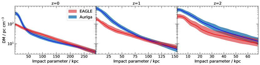
Figure 16: The dispersion measure of all four haloes in Eagle and Auriga at three redshifts, $z\sim 0,~{}1,~{}2$ from left to right, respectively. The dispersion measure, at fixed radius, $r$, for each halo is calculated by taking the median dispersion measure of many sightlines through a small annulus of depth $\mathrm{R}_{200}$. We also compute the lower and upper quartiles of the dispersion measure in each annulus. The solid line shows the mean of the median dispersion measure, at each radius, for all four haloes. The shaded region illustrates the range between the mean of the lower and upper quartiles for all the haloes. The dispersion measure at higher redshift is calculated in the frame of the halo at that redshift, not from an observer at the present day.

The dispersion measure is a measure of the free electron column density along a sightline and, potentially, one of the most useful metrics of the baryon content of the Local Group. As discussed in Section 3.4, CHIME is predicted to detect between $2$ and $40$ FRBs day^-1 over the whole sky (Connor et al., 2016). The hot halo of M31 makes a significant contribution to the dispersion measure of FRBs when their emission passes through the halo with an impact parameter of $\leq 150~{}\mathrm{kpc}$; this corresponds to an angle of approximately $11\degree$ on the sky, assuming that M31 is $\sim 770~{}\mathrm{kpc}$ away from the MW. Therefore, M31 covers approximately $\sim 400~{}\mathrm{deg^{2}}$, or $\sim 1\%$ of the sky. This implies that the CHIME survey should expect to detect roughly between $10$ and $150$ FRB’s per year behind the M31 halo. These can be compared with sightlines adjacent to M31. If the foreground contribution from the MW is uniform, or at least smooth over a narrow range of viewing angles, and the FRB population has the same redshift distribution over this range, the differences in these dispersion measures will be a direct reflection of the properties of the plasma in M31. The contribution of M31 to the dispersion measure can then be used to infer the amount of hot gas present in M31 and, thus, to constrain its baryon fraction.

In this section we compute the dispersion measure from several thousand random sightlines through the four primary MW-like haloes at three redshifts, $z=0,~{}1,~{}2$. The electron column density is calculated for parallel sightlines as described in Section 7.1. These are projected directly through $2\times\mathrm{R}_{200}$ of the primary halo at varying impact parameters. The dispersion measure at a given radius of each halo is calculated by taking the median of many sightlines in a small annulus. We project through the $x$, $y$ and $z$ axes and combine the results. Additionally we compute the lower and upper quartiles in each annulus.

The dispersion measure profiles in Fig. 16 represent idealized observations of M31 from Earth, with contributions from the MW and material beyond M31 removed (i.e. the IGM and other distant haloes). In practice, we expect the contribution from halo gas in M31 to be large, and thus to be readily detectable when compared with sightlines that do not pass through M31. Although they are not realistic mocks of observations from Earth, the results in Fig. 16 provide some insight into how the dispersion measure of a halo varies with impact parameter and redshift, and thus may help interpret observational data. Later in this section, we discuss how future work could improve the realism of the simulated profiles and how they could be used to exploit the constraining power of future observations.

With current data it is only possible to make direct measurements of today’s dispersion measure around M31 and other Local Group. We do, however, include results from higher redshifts in Fig. 16 to understand how the dispersion measure evolves and to give insight on the possible background contributions to observations. (The dispersion measure at higher redshift is calculated in the frame of the halo at that redshift, not from an observer at the present day.)

At the present day, both simulations predict a similar trend, with the dispersion measure being highest in the central regions and declining with increasing impact parameter. At $z=0$, the dispersion measure typically drops from a peak value of $\geq 10^{2}~{}\mathrm{pc~{}cm^{-3}}$ in the centre of the halo to $\sim 1~{}\mathrm{pc~{}cm^{-3}}$ at $\mathrm{R}_{200}$, and continues to fall beyond this radius (not shown in the figure). Beyond the inner $50~{}\mathrm{kpc}$, Eagle  and Auriga predict similar profiles. The main difference occurs in the centre of the halo. In Eagle the dispersion measure decreases with impact parameter at an almost constant rate. In Auriga there is a peak at the very centre which drops rapidly out to $50~{}\mathrm{kpc}$. Beyond that, both the slope and amplitude of the profiles in the two simulations are approximately equal.

The peak in the dispersion measure in the inner regions of Auriga is also present at higher redshifts. At $z\geq 1$ a similar peak, but of lower amplitude, also appears in the Eagle simulations. The peak at the centre of the Auriga haloes at all redshifts coincides with the peak in the column densities of the ions that trace the warm-hot gas within the CGM (see Fig. 15) Thus, the origin of this large dispersion measure is plausibly the same as that of the ions. Feedback produces hot, metal-enriched, centrally-concentrated gas which is dense. This gas then cools, at an almost constant density, before rejoining the ISM. The electron mass will trace the gas mass in Fig. 11 (a). It is the hot gas of atomic density $\geq 0.001~{}\mathrm{cm^{-3}}$ in Auriga that produces the centrally concentrated dispersion measure peak. This gas is not present in Eagle at $z=0$ and, as a result, the profile is much flatter near the centre.

At higher redshift, Auriga predicts a higher dispersion measure throughout the halo. This behaviour is similar to that of the column densities of Ne vi, Ne viii, OVI and O vii in the central regions seen in Fig. 15, which typically probe gas at temperature $\sim 10^{5.5}~{}\mathrm{K}$. The difference in baryon mass in the haloes of Eagle and Auriga drives the difference in the amplitude of the dispersion measure profiles.

At lower redshift, the baryon fraction of the Auriga haloes is still a factor of two higher than the Eagle counterparts. However, the dispersion measure in two simulations tends to agree reasonably well outside of the central region, $\geq 50~{}\mathrm{kpc}$. Inside the central region, the Auriga haloes boast significantly higher dispersion measure, thus indicating that the extra baryonic mass in Auriga, at present-day, is centrally concentrated. Efficient galactic fountains in Auriga can continuously produce centrally concentrated hot gas.

In summary, the dispersion measure is a measure of the amount of ionised gas along the line-of-sight and is strongly sensitive to the distribution of hot gas around MW-mass haloes, which is mostly ionised. The similar dispersion measure profiles in the outer regions of Eagle and Auriga at $z=0$ imply that the haloes in the two simulations have similar amounts of hot gas in this region, despite having large differences in baryon fraction. This is possible as the extra baryons present in Auriga are centrally concentrated due to the galactic fountains, which leads to a large central peak in the dispersion measure profile in Auriga.

We predict that future surveys of dispersion measure inferred from FRBs should be able to identify or exclude the existence of a galactic fountain in either the MW or M31, through analysis of dispersion measure variation with impact parameter within the central regions. We also expect that the background, e.g. the contributions from the IGM and other intervening haloes at higher redshift, should be larger if there are hot, spatially extended outflows at high redshift, such as those found in Eagle. It may also be possible to identify the presence of a hot galactic fountain by direct observation of X-ray emission (Oppenheimer et al., 2020b).

In this analysis, we did not include material which is part of the ISM. When calculating the free electron density we discarded gaseous material with an atomic number density $\geq 0.1~{}\mathrm{cm^{-1}}$ or a temperature $\leq 10^{4}~{}\mathrm{K}$. Gas in this regime is not modelled explicitly in the simulations, however the distribution and morphology of the cold gas is in reasonable agreement with observations (Marinacci et al., 2017). The dispersion measure profiles in the innermost regions may well be higher than predicted in this work due to dispersion by ISM gas. However, predictions for the ISM suggest that it contributes only $\leq 50~{}\mathrm{pc~{}cm^{-3}}$ (Lorimer et al., 2007); thus the central regions should be dominated by contributions from halo gas.

Finally, we stress that realistic mock catalogues will be needed to interpret future data. Constructing these will require combining high-resolution Local Group simulations such as those presented here with large-volume cosmological simulations to determine the expected background.

7.3 Comparing to current observations

In this section we compare our preliminary mock observations of the column densities of Ne viii for our sample of four MW-mass haloes with current observations. The COS-Halos survey (Tumlinson et al., 2013) and CASBaH survey (Burchett et al., 2019) are absorption line studies of galaxies in the UV. They typically cover the redshift range $0.05<z<1.5$ and provide information on column densities and covering fractions of H i, Ne viii and O vi. Burchett et al. (2019) collated a statistical sample of Ne viii CGM absorbers. This sample includes 29 CGM systems in the redshift range $z=0.5-1.5$, with a median redshift, $z=0.68$, stellar masses in the range $10^{9.5}-10^{11.5}~{}\mathrm{\mathrm{M}_{\odot}}$ and impact parameters within $450~{}\mathrm{kpc}$ of the central galaxy.

In Fig. 17 we compare the column density of Ne viii, as in Fig. 15, at $z=0.5$ for both Eagle and Auriga, with observational data, including both the detections (solid black circles) and non-detections (empty triangles) of Burchett et al. (2019). The highest inferred column density of Ne viii is $14.98\pm 0.09~{}\mathrm{cm^{-2}}$ at an impact parameter of $69~{}\mathrm{kpc}$ and redshift, $z=0.93$. The central galaxy of this system has an estimated stellar mass of $10^{11.2}~{}\mathrm{\mathrm{M}_{\odot}}$, slightly larger than our simulated galaxies. This high observed column density is larger than found in any of the predictions of Eagle and Auriga, as seen in the figure. However, column densities this high are not uncommon at lower impact parameters in Auriga.

The column densities at slightly larger radii, $100-200~{}\mathrm{kpc}$, are consistent with the predictions of both simulations, with almost all of the observational detections in this range overlapping the results from our simulations within the uncertainties. In the outer regions, the observations are dominated by upper limits which are higher than, and thus consistent with the inferred column densities in the simulations.

The observations follow the general trend that the inner regions are dominated by detections of $\approx 10^{14}~{}\mathrm{cm^{-2}}$, whereas the outer regions are mostly upper limits between $\approx 10^{13.5}-10^{14}~{}\mathrm{cm^{-2}}$. This is suggestive of a Ne viii column density profile which typically declines by $\geq 0.5~{}\mathrm{dex}$ between an impact parameter of $150~{}\mathrm{kpc}$ and $300~{}\mathrm{kpc}$. This is also seen in both Eagle and Auriga. Eagle  better recovers the (approximately) flat distribution of Ne viii detections; however, Auriga agrees better with the higher central column densities. In any case, the model preferences are driven by two data points, the ones with the lowest and highest impact parameters. Therefore the model choice is subjective, and there is no clear preference towards either Eagle or Auriga.

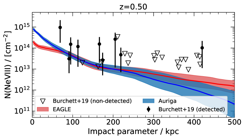
Figure 17: The atomic column number density of Ne viii as a function of impact parameter from the centre of the primary halo in both the Eagle (red) and Auriga (blue) simulations out to $500~{}\mathrm{kpc}$ at $z=0.5$. The column density at a fixed radius, $r$, for a single halo is calculated by taking the median column density of many sightlines through a small annulus. We also compute the lower and upper quartiles of the column density in each annulus. The solid line shows the mean of the median column density, at each radius, for all four haloes. The shaded region illustrates the range between the mean of the lower, and upper quartiles, for all of the haloes sampled. We also include the observational detections (solid black circles) and non-detections (empty triangles) of Burchett et al. (2019).

8 Discussion and Conclusions

The two simulations that we have analysed in this work have been shown to reproduce many galaxy observables even though they involve different galaxy formation models and hydrodynamical schemes. In particular the large-volume Eagle simulations reproduce the galaxy stellar mass function (Schaye et al., 2015), the evolution of galaxy masses (Furlong et al., 2015), sizes (Furlong et al., 2017) and colours (Trayford et al., 2015). Similarly, large volume simulations with a similar model to Auriga have successfully reproduced the scaling relations and evolution of galaxy sizes (Genel et al., 2018), the formation of realistic disc galaxies (Pillepich et al., 2018), the gas-phase mass-metallicity relation (Torrey et al., 2019) and the diversity of kinematic properties observed in the MW-type galaxies (Lovell et al., 2018).

In this work, we have analysed the emergent baryon cycle around two Local Group-like volumes centred around a pair of haloes similar to those of the MW and M31. We investigated how the baryon cycle differed when using the different subgrid models of the Eagle and Auriga simulations. While these models are similar, they have significantly different implementations of SNe feedback. Eagle injects all the energy from SNe in the form of a thermal energy ‘dump’, whereas Auriga uses hydrodynamically decoupled ‘wind’ particles that carry mass, energy, momentum and metals away from the ISM to lower density regions of the galactic halo.

In Section 4, we explored the effects of the different feedback implementations on baryonic evolution, particularly the baryon fraction, in and around the two primary haloes as a function of time. We found the minimum baryon fraction within a sphere around a primary Eagle galaxy to be $\approx 40\%$ of the cosmic baryon budget, which is approximately half the value found in Auriga. Furthermore, the Eagle simulations exhibit a baryon deficiency of $\geq 10\%$ within a radius $\geq 1~{}\mathrm{Mpc}$ (comoving) of the halo, extending to $\approx 2~{}\mathrm{Mpc}$ at the present day. Thus, in Eagle, the Local Group is a baryon deficient environment. Conversely, in the Auriga simulations the baryon fraction is within $5\%$ of unity at all radii $\geq 0.5~{}\mathrm{Mpc}$ (comoving), and at all redshifts. This difference in the baryon evolution is remarkable given that both simulations use the exact same initial conditions and produce central galaxies with relatively similar stellar properties. This is consistent with the findings of Mitchell & Schaye (2021) which show the gas mass, and thus density, of the CGM are more sensitive to the baryon cycle than is the case for the properties of the central galaxy.

In Section 5 we conducted a census of all the baryons expected to lie within $\mathrm{R}_{200}$ at the present day due to gravitational forces alone (which we called ‘predestined’). In Eagle we found that $\sim 35\%$ of the baryonic counterparts of the $z=0$ dark matter halo particles inhabit the primary halo, whereas in Auriga approximately $70\%$ do. Furthermore, in Eagle we found that almost half of the baryon counterparts of dark matter particles that are missing never entered the halo: they are ‘impeded’. By contrast, in Auriga almost $90\%$ of the absent baryons entered the halo before being ejected.

We also found that the physical extent of ejected and impeded baryons, in both Eagle and Auriga is such that there is baryonic mixing between the two primary haloes. This baryonic mass transfer, shown in Fig. 10, indicates that the presence of M31 may influence the evolution of the MW and viceversa (see Borrow et al., 2020).

The large ‘impeded’ gas component in Eagle is produced by halo-scale fast outflows with high covering fractions. The Auriga simulations do not produce sufficiently large outflows to impede accretion significantly. However, SNe feedback in both, Eagle and Auriga inject a similar amount of energy per unit mass into the surrounding gas. Thus, the different fates of the energetic gas must result from the method of injecting the energy, or the subsequent evolution of the gas (followed with two different hydrodynamical scheme.). We strongly suspect that it is the former that is responsible for the different outcomes.

This differences in the SNe subgrid prescriptions in Eagle and Auriga  result in the post-SNe temperature of the gas in Eagle being much higher that in Auriga and, crucially, greater than $10^{7}~{}\mathrm{K}$. Thus, in Eagle radiative cooling is inefficient and the gas expands adiabatically. This expansion produces hot, low-density parcels of gas which are buoyant and accelerate outwards through the halo (Bower et al., 2016). Conversely, in Auriga  the lower post-SNe temperature makes radiatively cooling more efficient and the gas cools rapidly, at almost constant density, and recycles on a short timescale.

To summarise, we have found that the processes that regulate the rate of star formation in a MW-mass galaxy can be classified into two broad categories: ejective and preventative. The Auriga simulations are dominated by ejective feedback with relatively short recycling times, regulating star formation without significantly reducing the halo baryon fraction. However, in Eagle feedback at high redshift ejects a large mass of gas beyond $\mathrm{R}_{200}$. This gas has such a large covering fraction and outward pressure that it can suppress the cosmological accretion of gas. These findings are consistent with the results from the large volume Eagle simulations (Mitchell et al., 2019; Mitchell et al., 2020b) and the NIHAO simulations (Tollet et al., 2019) which all identify reduced cosmic gas accretion rates due to feedback processes. The FIRE simulations (Muratov et al., 2015) present some evidence that bursts of star formation at high redshift can suppress gas accretion into the inner halo; however, it is not clear if this suppression extends to $\mathrm{R}_{200}$ or low redshift. The FIRE simulations also produce (almost) baryonically closed MW-mass haloes (Hafen et al., 2019), thus more closely resembling those in Auriga, than Eagle. These results highlight a fundamental difference in the outcome of the feedback processes in various subgrid implementations.

A caveat is that the stellar mass of the central galaxies in Eagle is typically a factor of two lower than in Auriga. In principle, we could ‘tune’ the feedback parameters in Eagle to produce more massive galaxies in $10^{12}~{}\mathrm{\mathrm{M}_{\odot}}$ haloes and still end up with baryon-deficient haloes due to preventative feedback. Schaller et al. (2015) demonstrates that the ‘weak SNe’ Eagle variant can produce MW-mass haloes with stellar masses consistent with the Auriga galaxies, albeit with weaker feedback than used in Auriga. Furthermore, Wright et al. (2020) show that the rate of gas accretion at $\mathrm{R}_{200}$ for the same ‘weak SNe’ simulation differs from the Eagle reference model used in this work by less than $20\%$. Thus, the Eagle ‘weak SNe’ simulation produces Auriga-mass galaxies, while still suppressing cosmological gas accretion as shown in this work.

While we identify SNe feedback as the leading cause of differences in the baryon cycle around our simulated galaxies, there are other differences in the two simulations that could contribute. Namely, both simulations use different hydrodynamical solvers; however Schaller et al. (2015) and Hopkins et al. (2018) have demonstrated that the treatment of feedback is more significant in determining the outcome of simulations of this kind than the details of the hydrodynamics solver. Eagle and Auriga also use different implementations of AGN feedback. However, there is evidence to suggest that the effects of these AGN models on the gaseous baryon cycle are subdominant for haloes of mass $\sim 10^{12}~{}\mathrm{\mathrm{M}_{\odot}}$. van de Voort et al. (2021) shows the total gas mass within the virial radius of a MW-mass halo simulated with the Auriga model both with and without AGN feedback differ by only a few percent. However, the inclusion of AGN feedback decreases the $z=0$ stellar mass by $\sim 30\%$. Davies et al. (2020) show that AGN feedback in the Eagle reference model injects four times less energy than SNe in $\sim 10^{12}~{}\mathrm{\mathrm{M}_{\odot}}$ haloes. Furthermore, Figure 11 of Crain et al. (2015) shows the growth of black holes in the ‘ViscLo‘ AGN model in Eagle, used in this work, is significantly reduced relative to the reference model. As a result of this, the present-day black hole masses in the Eagle haloes presented in this work are all $\leq 10^{6.8}~{}\mathrm{\mathrm{M}_{\odot}}$ and therefore appear to have no significant effect on the baryon fraction of the haloes (Bower et al., 2017). However, Davies et al. (2020) and Oppenheimer et al. (2020a) demonstrate that AGN feedback can significantly reduce the baryon fraction of MW-mass haloes which host black holes of mass $\geq 10^{7.0-7.3}~{}\mathrm{\mathrm{M}_{\odot}}$.

In Section 7 we investigated the observable signatures of strong, accretion-impeding outflows in Eagle and efficient galactic fountains in Auriga. We concluded that the Eagle simulations produce almost flat column density profiles of ions which probe hot gas –Ne vi, Ne viii, O vi, O vii, O viii and Mg x– out to radii $\sim 3\mathrm{R}_{200}$ between $z=0-3$. These flat profiles are a signature of hot, outflowing gas driven by SNe within the central galaxy. In contrast, the Auriga simulations predict rapidly declining column densities with radius, as the SNe driven outflows are unable to eject large amounts of hot gas to such large radii. We attempted to constrain the two subgrid models by comparing to the data on Ne viii presented by Burchett et al. (2019). Unfortunately, these data are not constraining due to the small number of detections at very small and very large impact parameters.

We also investigated the dispersion measure, which probes the integrated free electron density along the line-of-sight. We found that the main difference between the dispersion measure profiles in Auriga and Eagle is also at the very centre. In Auriga, there is a peak at impact parameter $\leq 50~{}\mathrm{kpc}$, not found in Eagle. The dispersion measure is a promising observational diagnostic of the evolution of baryons around galaxies. A combination of high-resolution Local Group analogues, like those presented in this work, and large-volume cosmological simulations would facilitate the production of more realistic mock catalogues of FRBs. Large cosmological volumes allow modelling random sightlines out to the typical FRB redshifts, $z\sim 2$. These background contributions can be added to predictions from Local Group analogues to make realistic mocks of what would be seen from the Earth when looking, for example, in the direction of M31. These can be compared with real sightlines in the direction of M31 and just adjacent to it. As future surveys should detect hundreds of FRBs per year behind M31, these observations should be able to constrain models and shed light on the dominant processes involved in the galactic baryon cycle.

To conclude, we find that ejective and preventative feedback work in tandem to reduce the amount of gas within haloes in the Eagle galaxy formation model. In Auriga, MW-mass galactic haloes are almost ‘baryonically closed’, as ejective feedback beyond $\mathrm{R}_{200}$ typically re-accretes and does not significantly impede further cosmic gas accretion. Future observations of FRBs and CGM ion absorption should provide valuable data to compare and constrain different galaxy formation models. Dwarf galaxies may also provide a suitable laboratory for studying the baryon cycle. In particular, Fig. 2 shows there are significant differences in the stellar-mass/halo-mass relation of lower mass galaxies in the two models; these differences carry over into the baryon fraction of these objects. It is also likely that the size of the heated gas coronae around haloes within the Local Group will affect the number of star-free dark matter haloes, which are even less massive than dwarf galaxies, in the local environment (Benítez-Llambay et al., 2017; Sykes et al., 2019).

Software Citations

This paper made use of the following software packages:

• gadget (Springel, 2005)

• Arepo (Springel, 2010)

• python (Van Rossum & Drake, 2009), with the libraries:

  • numpy (van der Walt et al., 2011)

  • scipy (Jones et al., 2001)

  • h5py (Collette, 2013)

  • matplotlib (Hunter, 2007)

  • numba (Lam et al., 2015)

  • unyt (Goldbaum et al., 2018)

Appendix A Stellar disc properties

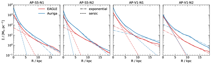
Figure 18: The radial stellar surface density profiles of the four primary haloes. The surface densities are calculated using all the stellar particles within a physical height of $\pm 5~{}\mathrm{kpc}$ from the galactic plane; these are shown as solid lines. The radial profiles are simultaneously fit with a Sersic (dashed) and exponential (dashed-dotted) profile using a non-linear least-squares method. Results for the Eagle and Auriga simulations are shown in red and blue respectively. The best-fit parameters may be found in Table 1.

Fig. 18 shows stellar surface density profiles, for stellar mass within $\pm 5~{}\mathrm{kpc}$ of the mid plane in the vertical direction, for all simulations at $z=0$. The profiles are simultaneously fit with a linear sum of an exponential profile of scale radius, $R_{\rm{D}}$, and a Sersic profile of the form $\exp(R/R_{\rm{eff}})^{n}$ (Sérsic, 1963). The best fit values are calculated using the least squares method to logarithm density profile.

References

- Anderson & Bregman (2010) Anderson M. E., Bregman J. N., 2010, ApJ, 714, 320
- Baugh (2006) Baugh C., 2006, Rep. Progress Phys., 69
- Behroozi et al. (2013) Behroozi P. S., Wechsler R. H., Conroy C., 2013, ApJ, 770, 57
- Benítez-Llambay et al. (2017) Benítez-Llambay A., et al., 2017, MNRAS, 465, 3913
- Bird et al. (2013) Bird S., Vogelsberger M., Sijacki D., Zaldarriaga M., Springel V., Hernquist L., 2013, MNRAS, 429, 3341
- Booth & Schaye (2009) Booth C. M., Schaye J., 2009, MNRAS, 398, 53
- Borrow et al. (2020) Borrow J., Anglés-Alcázar D., Davé R., 2020, MNRAS, 491, 6102
- Bower et al. (2016) Bower R. G., Schaye J., Frenk C. S., Theuns T., Schaller M., Crain R. A., McAlpine S., 2016, Monthly Notices of the Royal Astronomical Society, 465, 32
- Bower et al. (2017) Bower R. G., Schaye J., Frenk C. S., Theuns T., Schaller M., Crain R. A., McAlpine S., 2017, MNRAS, 465, 32
- Bregman et al. (2018) Bregman J. N., Anderson M. E., Miller M. J., Hodges-Kluck E., Dai X., Li J.-T., Li Y., Qu Z., 2018, ApJ, 862, 3
- Brooks et al. (2009) Brooks A. M., Governato F., Quinn T., Brook C. B., Wadsley J., 2009, ApJ, 694, 396
- Burchett et al. (2019) Burchett J. N., et al., 2019, ApJ, 877, L20
- Callingham et al. (2019) Callingham T. M., et al., 2019, MNRAS, 484, 5453
- Collette (2013) Collette A., 2013, Python and HDF5. O’Reilly
- Connor et al. (2016) Connor L., Lin H.-H., Masui K., Oppermann N., Pen U.-L., Peterson J. B., Roman A., Sievers J., 2016, MNRAS, 460, 1054
- Cordes & Chatterjee (2019) Cordes J. M., Chatterjee S., 2019, ARA&A, 57, 417
- Crain et al. (2009) Crain R. A., et al., 2009, MNRAS, 399, 1773
- Crain et al. (2015) Crain R. A., et al., 2015, MNRAS, 450, 1937
- Cullen & Dehnen (2010) Cullen L., Dehnen W., 2010, MNRAS, 408, 669
- Dalla Vecchia & Schaye (2008) Dalla Vecchia C., Schaye J., 2008, MNRAS, 387, 1431
- Dalla Vecchia & Schaye (2012) Dalla Vecchia C., Schaye J., 2012, MNRAS, 426, 140
- Davies et al. (2019) Davies J. J., Crain R. A., McCarthy I. G., Oppenheimer B. D., Schaye J., Schaller M., McAlpine S., 2019, MNRAS, 485, 3783
- Davies et al. (2020) Davies J. J., Crain R. A., Oppenheimer B. D., Schaye J., 2020, MNRAS, 491, 4462
- Davis et al. (1985) Davis M., Efstathiou G., Frenk C. S., White S. D. M., 1985, ApJ, 292, 371
- DeFelippis et al. (2017) DeFelippis D., Genel S., Bryan G. L., Fall S. M., 2017, ApJ, 841, 16
- Dolag et al. (2009) Dolag K., Borgani S., Murante G., Springel V., 2009, MNRAS, 399, 497
- Faerman et al. (2017) Faerman Y., Sternberg A., McKee C. F., 2017, ApJ, 835, 52
- Fattahi et al. (2016) Fattahi A., et al., 2016, MNRAS, 457, 844
- Ferland et al. (2013) Ferland G. J., et al., 2013, Rev. Mex. Astron. Astrofis., 49, 137
- Flynn et al. (2006) Flynn C., Holmberg J., Portinari L., Fuchs B., Jahreiß H., 2006, MNRAS, 372, 1149
- Frenk et al. (1988) Frenk C. S., White S. D. M., Davis M., Efstathiou G., 1988, ApJ, 327, 507
- Furlong et al. (2015) Furlong M., et al., 2015, MNRAS, 450, 4486
- Furlong et al. (2017) Furlong M., et al., 2017, MNRAS, 465, 722
- Genel et al. (2013) Genel S., Vogelsberger M., Nelson D., Sijacki D., Springel V., Hernquist L., 2013, MNRAS, 435, 1426
- Genel et al. (2018) Genel S., et al., 2018, MNRAS, 474, 3976
- Gingold & Monaghan (1977) Gingold R. A., Monaghan J. J., 1977, MNRAS, 181, 375
- Goldbaum et al. (2018) Goldbaum N. J., ZuHone J. A., Turk M. J., Kowalik K., Rosen A. L., 2018, Journal of Open Source Software, 3, 809
- Grand et al. (2017) Grand R. J. J., et al., 2017, MNRAS, 467, 179
- Grand et al. (2019) Grand R. J. J., et al., 2019, MNRAS, 490, 4786
- Gupta et al. (2012) Gupta A., Mathur S., Krongold Y., Nicastro F., Galeazzi M., 2012, ApJ, 756, L8
- Gupta et al. (2014) Gupta A., Mathur S., Galeazzi M., Krongold Y., 2014, Ap&SS, 352, 775
- Haardt & Madau (2012) Haardt F., Madau P., 2012, ApJ, 746, 125
- Hafen et al. (2019) Hafen Z., et al., 2019, MNRAS, 488, 1248
- Hayward et al. (2014) Hayward C. C., Torrey P., Springel V., Hernquist L., Vogelsberger M., 2014, MNRAS, 442, 1992
- Henden et al. (2018) Henden N. A., Puchwein E., Shen S., Sijacki D., 2018, MNRAS, 479, 5385
- Hopkins (2013) Hopkins P. F., 2013, MNRAS, 428, 2840
- Hopkins et al. (2018) Hopkins P. F., et al., 2018, MNRAS, 480, 800
- Hou et al. (2019) Hou J., Lacey C. G., Frenk C. S., 2019, MNRAS, 486, 1691
- Hummels et al. (2017) Hummels C. B., Smith B. D., Silvia D. W., 2017, ApJ, 847, 59
- Hunter (2007) Hunter J. D., 2007, Computing in Science & Engineering, 9, 90
- Jenkins (2010) Jenkins A., 2010, MNRAS, 403, 1859
- Jones et al. (2001) Jones E., Oliphant T., Peterson P., et al., 2001, SciPy: Open source scientific tools for Python, http://www.scipy.org/
- Katz & Gunn (1991) Katz N., Gunn J. E., 1991, ApJ, 377, 365
- Katz et al. (1992) Katz N., Hernquist L., Weinberg D. H., 1992, ApJ, 399, L109
- Kelly et al. (2020) Kelly A. J., Jenkins A., Frenk C. S., 2020, The origin of X-ray coronae around simulated disc galaxies (arXiv:2005.12926)
- Kereš et al. (2005) Kereš D., Katz N., Weinberg D. H., Davé R., 2005, MNRAS, 363, 2
- Kereš et al. (2012) Kereš D., Vogelsberger M., Sijacki D., Springel V., Hernquist L., 2012, MNRAS, 425, 2027
- Lacey & Cole (1994) Lacey C., Cole S., 1994, MNRAS, 271, 676
- Lam et al. (2015) Lam S. K., Pitrou A., Seibert S., 2015, in Proceedings of the Second Workshop on the LLVM Compiler Infrastructure in HPC. LLVM ’15. ACM, New York, NY, USA, pp 7:1–7:6, doi:10.1145/2833157.2833162, %****␣main.bbl␣Line␣350␣****http://doi.acm.org/10.1145/2833157.2833162
- Larson (1974) Larson R. B., 1974, MNRAS, 169, 229
- Le Brun et al. (2014) Le Brun A. M. C., McCarthy I. G., Schaye J., Ponman T. J., 2014, MNRAS, 441, 1270
- Li & Bregman (2017) Li Y., Bregman J., 2017, ApJ, 849, 105
- Licquia & Newman (2015) Licquia T. C., Newman J. A., 2015, The Astrophysical Journal, 806, 96
- Lorimer et al. (2007) Lorimer D. R., Bailes M., McLaughlin M. A., Narkevic D. J., Crawford F., 2007, Science, 318, 777
- Lovell et al. (2018) Lovell M. R., et al., 2018, MNRAS, 481, 1950
- Lucy (1977) Lucy L. B., 1977, AJ, 82, 1013
- Madau & Dickinson (2014) Madau P., Dickinson M., 2014, Annual Review of Astronomy and Astrophysics, 52, 415
- Marinacci et al. (2017) Marinacci F., Grand R. J. J., Pakmor R., Springel V., Gómez F. A., Frenk C. S., White S. D. M., 2017, MNRAS, 466, 3859
- Mathews & Baker (1971) Mathews W. G., Baker J. C., 1971, ApJ, 170, 241
- McMillan (2011) McMillan P. J., 2011, MNRAS, 414, 2446
- McQuinn (2014) McQuinn M., 2014, ApJ, 780, L33
- Miller & Bregman (2015) Miller M. J., Bregman J. N., 2015, ApJ, 800, 14
- Mitchell & Schaye (2021) Mitchell P. D., Schaye J., 2021, arXiv e-prints, p. arXiv:2103.10966
- Mitchell et al. (2019) Mitchell P. D., Schaye J., Bower R. G., Crain R. A., 2019, arXiv e-prints, p. arXiv:1910.09566
- Mitchell et al. (2020a) Mitchell P. D., Schaye J., Bower R. G., Crain R. A., 2020a, MNRAS, 494, 3971
- Mitchell et al. (2020b) Mitchell P. D., Schaye J., Bower R. G., 2020b, MNRAS, 497, 4495
- Muratov et al. (2015) Muratov A. L., Kereš D., Faucher-Giguère C.-A., Hopkins P. F., Quataert E., Murray N., 2015, MNRAS, 454, 2691
- Navarro & Benz (1991) Navarro J. F., Benz W., 1991, ApJ, 380, 320
- Navarro & White (1993) Navarro J. F., White S. D. M., 1993, MNRAS, 265, 271
- Navarro & White (1994) Navarro J. F., White S. D. M., 1994, MNRAS, 267, 401
- Navarro et al. (1995) Navarro J. F., Frenk C. S., White S. D. M., 1995, MNRAS, 275, 720
- Navarro et al. (1997) Navarro J. F., Frenk C. S., White S. D. M., 1997, ApJ, 490, 493
- Nelson et al. (2013) Nelson D., Vogelsberger M., Genel S., Sijacki D., Kereš D., Springel V., Hernquist L., 2013, MNRAS, 429, 3353
- Nelson et al. (2015) Nelson D., Genel S., Vogelsberger M., Springel V., Sijacki D., Torrey P., Hernquist L., 2015, MNRAS, 448, 59
- Nelson et al. (2018) Nelson D., et al., 2018, MNRAS, 475, 624
- Nelson et al. (2019) Nelson D., et al., 2019, Computational Astrophysics and Cosmology, 6, 2
- Oppenheimer et al. (2010) Oppenheimer B. D., Davé R., Kereš D., Fardal M., Katz N., Kollmeier J. A., Weinberg D. H., 2010, MNRAS, 406, 2325
- Oppenheimer et al. (2020a) Oppenheimer B. D., et al., 2020a, MNRAS, 491, 2939
- Oppenheimer et al. (2020b) Oppenheimer B. D., et al., 2020b, ApJ, 893, L24
- Pearce et al. (1999) Pearce F. R., et al., 1999, ApJ, 521, L99
- Petroff (2017) Petroff E., 2017, arXiv e-prints, p. arXiv:1709.02189
- Pillepich et al. (2017) Pillepich A., et al., 2017, Monthly Notices of the Royal Astronomical Society, 473, 4077–4106
- Pillepich et al. (2018) Pillepich A., et al., 2018, MNRAS, 475, 648
- Planck Collaboration et al. (2013) Planck Collaboration et al., 2013, A&A, 557, A52
- Price (2008) Price D. J., 2008, Journal of Computational Physics, 227, 10040
- Price (2012) Price D. J., 2012, Journal of Computational Physics, 231, 759
- Rosas-Guevara et al. (2015) Rosas-Guevara Y. M., et al., 2015, MNRAS, 454, 1038
- Sales et al. (2012) Sales L. V., Navarro J. F., Theuns T., Schaye J., White S. D. M., Frenk C. S., Crain R. A., Dalla Vecchia C., 2012, MNRAS, 423, 1544
- Sawala et al. (2016) Sawala T., et al., 2016, MNRAS, 457, 1931
- Schaller et al. (2015) Schaller M., Dalla Vecchia C., Schaye J., Bower R. G., Theuns T., Crain R. A., Furlong M., McCarthy I. G., 2015, MNRAS, 454, 2277
- Schaye & Dalla Vecchia (2008) Schaye J., Dalla Vecchia C., 2008, MNRAS, 383, 1210
- Schaye et al. (2010) Schaye J., et al., 2010, MNRAS, 402, 1536
- Schaye et al. (2015) Schaye J., et al., 2015, MNRAS, 446, 521
- Sérsic (1963) Sérsic J. L., 1963, Boletin de la Asociacion Argentina de Astronomia La Plata Argentina, 6, 41
- Shull & Danforth (2018) Shull J. M., Danforth C. W., 2018, ApJ, 852, L11
- Sijacki et al. (2012) Sijacki D., Vogelsberger M., Kereš D., Springel V., Hernquist L., 2012, MNRAS, 424, 2999
- Smith et al. (2016) Smith B. D., et al., 2016, Grackle: Chemistry and radiative cooling library for astrophysical simulations (ascl:1612.020)
- Smith et al. (2018) Smith M. C., Sijacki D., Shen S., 2018, Monthly Notices of the Royal Astronomical Society, 478, 302
- Sommer-Larsen et al. (1999) Sommer-Larsen J., Gelato S., Vedel H., 1999, ApJ, 519, 501
- Springel (2005) Springel V., 2005, MNRAS, 364, 1105
- Springel (2010) Springel V., 2010, MNRAS, 401, 791
- Springel & Hernquist (2003) Springel V., Hernquist L., 2003, MNRAS, 339, 289
- Springel et al. (2001) Springel V., White S. D. M., Tormen G., Kauffmann G., 2001, MNRAS, 328, 726
- Sykes et al. (2019) Sykes C., Fumagalli M., Cooke R., Theuns T., Benítez-Llambay A., 2019, MNRAS, 487, 609
- Thacker & Couchman (2001) Thacker R. J., Couchman H. M. P., 2001, ApJ, 555, L17
- Tollet et al. (2019) Tollet É., Cattaneo A., Macciò A. V., Dutton A. A., Kang X., 2019, MNRAS, 485, 2511
- Torrey et al. (2012) Torrey P., Vogelsberger M., Sijacki D., Springel V., Hernquist L., 2012, MNRAS, 427, 2224
- Torrey et al. (2014) Torrey P., Vogelsberger M., Genel S., Sijacki D., Springel V., Hernquist L., 2014, MNRAS, 438, 1985
- Torrey et al. (2019) Torrey P., et al., 2019, MNRAS, 484, 5587
- Trayford et al. (2015) Trayford J. W., et al., 2015, MNRAS, 452, 2879
- Tumlinson et al. (2013) Tumlinson J., et al., 2013, ApJ, 777, 59
- Van Rossum & Drake (2009) Van Rossum G., Drake F. L., 2009, Python 3 Reference Manual. CreateSpace, Scotts Valley, CA
- Vogelsberger et al. (2012) Vogelsberger M., Sijacki D., Kereš D., Springel V., Hernquist L., 2012, MNRAS, 425, 3024
- Vogelsberger et al. (2013) Vogelsberger M., Genel S., Sijacki D., Torrey P., Springel V., Hernquist L., 2013, MNRAS, 436, 3031
- Vogelsberger et al. (2014a) Vogelsberger M., et al., 2014a, MNRAS, 444, 1518
- Vogelsberger et al. (2014b) Vogelsberger M., et al., 2014b, MNRAS, 444, 1518
- White & Frenk (1991) White S. D. M., Frenk C. S., 1991, ApJ, 379, 52
- White & Rees (1978) White S. D. M., Rees M. J., 1978, MNRAS, 183, 341
- Wiersma et al. (2009a) Wiersma R. P. C., Schaye J., Smith B. D., 2009a, Mon. Not. Roy. Astron. Soc., 393, 99
- Wiersma et al. (2009b) Wiersma R. P. C., Schaye J., Theuns T., Dalla Vecchia C., Tornatore L., 2009b, MNRAS, 399, 574
- Wijers et al. (2019) Wijers N. A., Schaye J., Oppenheimer B. D., Crain R. A., Nicastro F., 2019, MNRAS, 488, 2947
- Wijers et al. (2020) Wijers N. A., Schaye J., Oppenheimer B. D., 2020, MNRAS, 498, 574
- Wright et al. (2020) Wright R. J., Lagos C. d. P., Power C., Mitchell P. D., 2020, MNRAS, 498, 1668
- Zheng et al. (2014) Zheng Z., Ofek E. O., Kulkarni S. R., Neill J. D., Juric M., 2014, ApJ, 797, 71
- van de Voort et al. (2011a) van de Voort F., Schaye J., Booth C. M., Haas M. R., Dalla Vecchia C., 2011a, MNRAS, 414, 2458
- van de Voort et al. (2011b) van de Voort F., Schaye J., Booth C. M., Dalla Vecchia C., 2011b, MNRAS, 415, 2782
- van de Voort et al. (2021) van de Voort F., Bieri R., Pakmor R., Gómez F. A., Grand R. J. J., Marinacci F., 2021, MNRAS, 501, 4888
- van der Walt et al. (2011) van der Walt S., Colbert S. C., Varoquaux G., 2011, Computing in Science Engineering, 13, 22