FastAno: Fast Anomaly Detection
via Spatio-temporal Patch Transformation

Abstract

Video anomaly detection has gained significant attention due to the increasing requirements of automatic monitoring for surveillance videos. Especially, the prediction based approach is one of the most studied methods to detect anomalies by predicting frames that include abnormal events in the test set after learning with the normal frames of the training set. However, a lot of prediction networks are computationally expensive owing to the use of pre-trained optical flow networks, or fail to detect abnormal situations because of their strong generative ability to predict even the anomalies. To address these shortcomings, we propose spatial rotation transformation (SRT) and temporal mixing transformation (TMT) to generate irregular patch cuboids within normal frame cuboids in order to enhance the learning of normal features. Additionally, the proposed patch transformation is used only during the training phase, allowing our model to detect abnormal frames at fast speed during inference. Our model is evaluated on three anomaly detection benchmarks, achieving competitive accuracy and surpassing all the previous works in terms of speed.

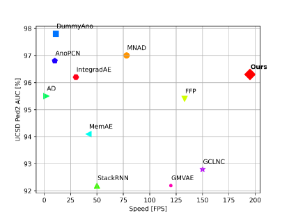
Figure 1: Comparison of evaluation speed (FPS) and frame-level AUC (%) in Ped2 test set. The methods compared in this figure are listed in Table 7. Our framework demonstrates state-of-the-art in terms of FPS and performs competitively with other methods.

1 Introduction

Video anomaly detection refers to the task of recognizing unusual events in videos. It has gained attention due to the implementation of video surveillance systems. Surveillance cameras are widely used for public safety. However, the monitoring capacity is not up to the mark. Since abnormal events rarely happen in the real world compared to normal events, automatic anomaly detection systems are in high demand to reduce the monitoring burden. However, it is very challenging because obtaining the datasets is difficult owing to the imbalance of events and variable definitions of abnormal events based on the context of each video.
One of the challenging factors of anomaly detection is the data imbalance problem, meaning that the abnormal scenes are more difficult to capture than normal scenes because of their scarcity in the real world. Therefore, datasets with an equal number of both types of scenes are hard to obtain, and consequently, only the normal videos are provided as training data [3]. This is known as an unsupervised approach for anomaly detection used by most of the previous works [13, 32, 39, 40]. The unsupervised network needs to learn the representative features of the unlabeled normal training set and sort the frames with outlying features to detect abnormal events. Autoencoder (AE) [14]-based methods [1, 51, 22] have proven to be successful for such a task. Frame predicting AEs [22, 43] and frame reconstructing AEs [33, 13] have been proposed assuming that anomalies that are unseen in the training phase cannot be predicted or reconstructed when the model is trained only on normal frames. However, these methods do not consider the drawback of AE—that AE may generate anomalies as clearly as normal events due to the strong generalizing capacity of convolutional neural networks (CNNs) [12]. To minimize this factor, Gong et al. [12] and Park et al. [34] proposed memory-based methods to use only the most essential features of normal frames for the generation. However, the memory-based methods are not efficient for videos with various scenes because their performance is highly dependent on the number of items. Many memory items are required to read and update patterns of various scenes, slowing down the detection.
Another critical and challenging issue for video anomaly detection is the performing speed. The main purpose of anomaly detection is to detect abnormal events or emergencies immediately, but slow models do not meet this purpose. In the previous studies, the following factors are observed to slow down the detection speed: heavy pre-trained networks such as optical flow [22, 39, 40, 49], object detectors [10, 15], and pre-trained feature extractors [38, 42]. These modules are complex and computationally expensive.

Therefore, we take the detection speed into account and employ a patch transformation method that is used only during training. We implement this approach by artificially generating abnormal patches via applying transformations to patches randomly selected from the training dataset. We adopt spatial rotation transformation (SRT) and temporal mixing transformation (TMT) to generate a patch anomaly at a random location within a stacked frame cuboid. Given this anomaly-included frame cuboid, our AE is trained to learn the employed transformation and predict the upcoming normal frame. The purpose of SRT is to generate an abnormal appearance and encourage the model to learn spatially invariant features of normal events. For instance, when a dataset defines walking pedestrians as normal and all others as abnormal, by giving a sequence of a rotated person (e.g., upside-down, lying flat) and forcing the model to generate a normally standing person, the model learns normal patterns of pedestrians. TMT, which is shuffling the selected patch cube in the temporal axis to create abnormal motion, is intended to enhance learning temporally invariant features of normal events. Given a set of frames where an irregular motion takes place in a small area, the model has to learn how to rearrange the shuffled sequence in the right order to correctly predict the upcoming frame.
To the best of our knowledge, unlike [22, 12, 34, 39, 15, 38], our framework performs the fastest because there are no additional modules or pre-trained networks. Furthermore, the proposed patch transformation does not drop the speed because it is detached during detection. Likewise, we designed all components of our method considering the detection speed in an effort to make it suitable for anomaly detection in the real world.
We summarize our contributions as follows:

• We apply a patch anomaly generation phase to the training data to enforce normal pattern learning, especially in terms of appearance and motion.

• The proposed patch generation approach can be implemented in conjunction with any backbone network during the training phase.

• Our model performs at very high speed and at the same time achieves competitive performance on three benchmark datasets without any pre-trained modules (e.g, optical flow networks, object detectors, and pre-trained feature extractors).

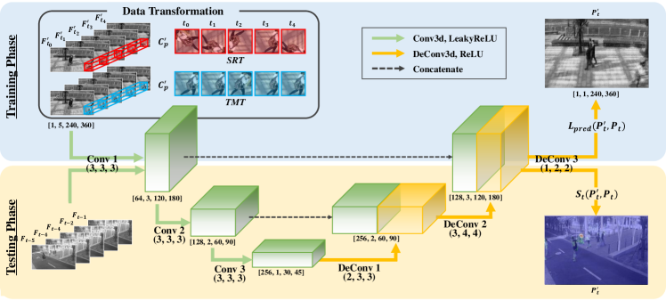
Figure 2: The overview of our framework. During the training phase, SRT and TMT are employed to make our input $\mathbf{C^{\prime}_{f}}$. The AE is trained to generate a succeeding frame that mimics the normal frame. During the testing phase, frames are fed into the AE and the corresponding output $\mathbf{P^{\prime}_{t}}$ is generated. The normality score $S_{t}(P^{\prime}_{t},P_{t})$ is used to discriminate abnormal frames. The $\mathbf{P^{\prime}_{t}}$ in this figure is a combination of $\mathbf{P^{\prime}_{t}}$ and a difference map for better understanding. The values in brackets indicate [channel, temporal, height, width] of feature and (depth, height, width) of the kernel in order.

2 Related work

2.1 AE-based approach

Frame predicting and reconstructing AEs have been proposed under the assumption that models trained only on normal data are not capable of predicting or reconstructing abnormal frames, because these are unseen during training. Some studies [22, 43, 34, 26] trained AEs that predict a single future frame from several successive input frames. Additionally, many effective reconstructing AEs [33, 51, 34, 5] have been proposed. Cho et al. [5] proposed two-path AE, where two encoders were used to model appearance and motion features. Focusing on the fact that abnormal events occur in small regions, patch-based AEs [51, 47, 33, 8], have been proposed. However, it has been observed that AEs tend to generalize well to generate abnormal events strongly, mainly due to the capacity of CNNs, which leads to missing out on anomalies during detection. To alleviate this drawback, Gong et al. [12] and Park et al. [34] suggested networks that employ memory modules to read and update memory items. These methods showcased outstanding performance on several benchmarks. However, they are observed to be ineffective for large datasets due to the limitation of memory size. Furthermore, some works [22, 39, 40, 38] have used optical flow to estimate motion features because information of temporal patterns is crucial in anomaly detection.

2.2 Transformation-based approach

Many image transformation methods, such as augmentations, have been proposed to increase recognition performance and robustness in varying environments in limited training datasets. This technique was first applied to image recognition and was later extended to video recognition. For the image-level modeling, Komodakis et al. [19] suggested unsupervised learning for image classification by predicting the direction of the rotated input. Krizhevsky et al. [20] used rotation, flipping, cropping, and color jittering to enhance learning spatially invariant features. Furthermore, DeVries et al. [7] devised CutOut, a method that deletes a box at a random location to prevent the model from focusing only on the most discriminative regions. Zhang et al. [52] proposed MixUp which blends two training data on both the images and the labels. Yun et al. [50] put forth a combination of CutOut and MixUp, called CutMix. For the video-level model, augmentation techniques have been extended to the temporal axis. Ji et al. [16] proposed a method called time warping and time masking, which randomly skips or adjusts temporal frames.
Several studies have used the techniques mentioned above for video anomaly detection based on the assumption that applying transformations to the input forces the network to embed critical information better. Zaheer et al. [51] suggested a pseudo anomaly module to create an artificial anomaly patch by blending two arbitrary patches from normal frames. They reconstructed both normal and abnormal patches and trained a discriminator to predict the source of the reconstructed output. Hasan et al. [13] and Zhao et al. [54] sampled the training data by skipping a fixed number of frames in the temporal axis. Moreover, Joshi et al. [17] generated abnormal frames from normal frames by cropping an object detected with a semantic segmentation model and placing it in another region in the frame to generate an abnormal appearance. Wang et al. [46] applied random cropping, flipping, color distortion, rotation, and grayscale to the entire frame. In contrast to these methods, our network embeds normal patterns by training from frames with anomaly-like patches. We transform the input frames along the spatial axis or temporal axis to generate abnormal frames within training datasets. Georgescu et al. [10] used sequence-reversed frames for a self-supervised binary classification task where the network guesses whether the given samples are regular or not. On the other hand, our method predicts the original frame from sequence transformed input and learns the normal patterns.

3 Proposed approach

This section presents an explicit description of our model formation. Our model consists of two main phases: (1) the patch anomaly generation phase and (2) the prediction phase.

3.1 Overall architecture

Fig. 2 presents the overview of our framework. During the training phase, we first load $n$ adjacent frames to make a frame cuboid. After that, we apply our patch anomaly generation to the frame cuboid, which is forwarded to the AE. Our AE extracts spatial and temporal patterns of the input and generates a future frame. During inference, the patch anomaly generation is not employed. A raw frame cuboid is fed as an input to the AE. The difference between the output of the AE and the ground truth frame is used as a score to judge normality.

3.2 Patch anomaly generation phase

Abnormal events in videos are categorized into two large branches: (1) anomalies regarding appearances (e.g., pedestrians on a vehicle road) and (2) anomalies regarding motion (e.g., an illegal U-turn or fighting in public). Hence, it is important to learn both the appearance and motion features of normal situations to detect anomalies in both cases.
The patch anomaly generation phase takes place before feeding the frames to the generator. We load $n$ successive frames $(\mathbf{F_{t},F_{t+1},F_{t+2},}\dots,\mathbf{F_{t+n-1}})$, resize each to $240\times 360$, and concatenate them on the temporal axis to form a 4D cuboid $\mathbf{C_{f}}\in\mathbb{R}^{C\times n\times 240\times 360}$, where $C$ denotes the number of channels for each frame. After that, we select a patch cuboid $\mathbf{C_{p}}\in\mathbb{R}^{C\times n\times 60\times 60}$ from a random location within $\mathbf{C_{f}}$ to apply transformation. Since anomalies usually occur in foregrounds, we exclude a margin of 12.5 percent in length from the top and bottom of the width of $\mathbf{C_{f}}$ from the selection area. We heuristically find that these marginal regions are generally backgrounds. Therefore, they commonly do not contain moving objects. Thus, by limiting the range, $\mathbf{C_{p}}$ is more likely to capture foregrounds than backgrounds, encouraging the model to concentrate on the moving objects. Then we apply SRT or TMT to $\mathbf{C_{p}}$ to form a transformed patch cuboid $\mathbf{C^{\prime}_{p}}$. Only one of the two is applied randomly for every input.
For SRT, each patch is rotated in a random direction between 0°, 90°, 180°, and 270°, following the approach of [19]. By forwarding these transformed frame cuboids $\mathbf{C^{\prime}_{f}}$ $(\mathbf{F^{\prime}_{t},F^{\prime}_{t+1},F^{\prime}_{t+2},}...,\mathbf{F^{\prime}_{t+n-1}})$ to the frame generator, our network is encouraged to focus on the abnormal region and recognize the spatial features of the normal appearances. Suppose a network is being trained on a dataset of people walking on a road. When it is given a frame cuboid with an upside-down person created by 180° rotation among all the other normal pedestrians and is programmed to predict a next normal scene, the network would learn the spatial features of a normal person, such as the head and the feet are generally placed at the top and bottom, respectively. Our SRT is demonstrated as follows:

$$SRT(\mathbf{F_{i}})=R(\mathbf{F}_{{\mathbf{i}}_{(x,y)\in[(x,x+W_{p}),(y,y+H_{p})]}},\delta_{i}),$$ (1)

where $R$ represents the rotation function for a patch within the pixel range of $[x,x+W_{p}]$ in the width axis and $[y,y+H_{p}]$ in the height axis of input frame $F_{i}$. $\delta_{i}$ denotes the randomly set direction for the ${i^{th}}$ frame, where $i$ is the index of the input frame in the range $[0,n-1]$. Furthermore, $W_{p}$ and $H_{p}$ represent the fixed width and height of the patch, respectively. The final $\mathbf{C^{\prime}_{f}}$ is generated by concatenating the transformed $\mathbf{F^{\prime}_{i}}$ in the temporal axis.
TMT involves shuffling the sequence of the patch cuboid $\mathbf{C_{p}}$ in the temporal axis with the intention of generating abnormal movement. The network needs to detect the awkward motion and match the sequence to normal before predicting the next frame to reduce the loss and generate a frame as similar as possible to the ground truth. For example, when the patch sequence is reversed, and a backward-walking person is generated within a frame where only forward walking people are annotated as normal, the model should find the correct sequence of the abnormal person based on the learned features to predict the correct trajectory. Our TMT function is as follows:

$$TMT(\mathbf{F_{i}})=T(\mathbf{F_{i}},\mathbf{F}_{\mathbf{\xi}_{{{i}_{(x,y)\in[(x,x+W_{p}),(y,y+H_{p})]}}}}),$$ (2)

where $T$ denotes a function that copies a patch located in pixel range of $[x,x+W_{p}]$ in the width axis and $[y,y+H_{p}]$ in the height axis of input frame $\mathbf{F_{\xi_{i}}}$ and pastes it to the $i^{th}$ frame. $\xi$ represents the shuffled sequence of $n$ patches (e.g. sequence $(4,1,0,3,2)$ when $n$ is 5). Same as SRT, the final $C^{\prime}_{f}$ is the stack of the transformed $F_{i}$.

Our patch anomaly generation phase is computationally cheaper than the other methods that embed spatio-temporal feature extraction in networks, such as storing and updating memory items [12, 34], and estimating optical flow with pre-trained networks [22, 39, 49, 2]. Therefore, our patch anomaly generation phase boosts feature learning at a low cost. Furthermore, this phase is not used during the inference, meaning that it does not affect the detection speed at all. Thus, our model is low in complexity and computational costs (see Section 4.3).

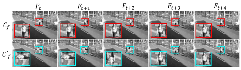
(a) SRT

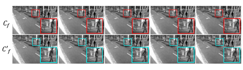
(b) TMT

Figure 3: Visualization of (a) SRT and (b) TMT. The frames in the upper rows are components of $C_{f}$. The regions marked in color are the locations of the selected $C_{p}$. The frames in the lower rows are data-transformed components of $C^{\prime}_{f}$.

3.3 AE architecture

The AE in our network aims to learn prototypical features of normal events and produce an output frame based on those features. Its main task is to predict $\mathbf{P_{t}}$—the frame coming after $\mathbf{C_{f}}$—from an input frame cuboid $\mathbf{C^{\prime}_{f}}$. Therefore, it is necessary to learn the temporal features as well as the spatial features to generate the frame with fine quality. The architecture of our model follows that of U-Net [41], in which the skip connections between the encoder and the decoder boost generation ability by preventing gradient vanishing and achieving information symmetry. The encoder consists of a stack of three-layer blocks that reduce the resolution of the feature map. We employ 3D convolution [44] to embed the temporal factor learning in our model. Specifically, the first block consists of one convolutional layer and one activation layer. The second and the last blocks are identical in structure: convolutional, batch normalization, and activation layers. The kernel size is set to $3\times 3\times 3$ for all three layers. The decoder also consists of a stack of three-layer blocks and is symmetrical to the encoder except that the convolutional layers are replaced by deconvolutional layers to upscale the feature map. In addition, we use leakyReLU activation [29] for the encoder and ReLU activation [31] for the decoder.
Likewise, the architecture of our AE is very simple compared to other previous studies, especially methods that employ pre-trained feature extractors [28, 42]. In that the running time is generally dependent on the simplicity of the model architecture, our AE is well designed, considering the speed.

3.4 Objective function and normality score

Prediction loss. Our model is trained to minimize the prediction loss. We use the $L1$ distance (Eq. (3)) and structural similarity index (SSIM) [45] loss (Eq. (4)) to measure the difference between the generated frame $\mathbf{P^{\prime}_{t}}$ and the ground truth frame $\mathbf{P_{t}}$. The $L1$ distance and SSIM demonstrate the difference of frames at the pixel-level and similarity at the feature-level, respectively. The functions are as follows:

$$L_{p}(\mathbf{P^{\prime}_{t}},\mathbf{P_{t}})=|\mathbf{P^{\prime}_{t}},\mathbf{P_{t}}|$$ (3)

$$L_{f}(\mathbf{P^{\prime}_{t}},\mathbf{P_{t}})=1-\frac{(2\mu_{\mathbf{P^{\prime}_{t}}}\mu_{\mathbf{P_{t}}}+c_{1})(2\sigma_{\mathbf{P^{\prime}_{t}}\mathbf{P_{t}}}+c_{2})}{(2\mu_{\mathbf{P^{\prime}_{t}}}^{2}\mu_{\mathbf{P_{t}}}^{2}+c_{1})(\sigma_{\mathbf{P^{\prime}_{t}}}^{2}+\sigma_{\mathbf{P_{t}}}^{2}+c_{2})},$$ (4)

where $\mu$ and $\sigma^{2}$ denote the average and variance of each frame, respectively. Furthermore, $\sigma_{\mathbf{P^{\prime}_{t}}\mathbf{P_{t}}}$ represents the covariance. $c_{1}$ and $c_{2}$ denote variables to stabilize the division. Following the work of Zhao et al. [53], we exploit a weighted combination of the two loss functions in our objective function as shown in Eq. (5).

$$L_{pred}(\mathbf{P^{\prime}_{t}},\mathbf{P_{t}})=\omega_{p}L_{p}(\mathbf{P^{\prime}_{t}},\mathbf{P_{t}})+\omega_{f}L_{f}(\mathbf{P^{\prime}_{t}},\mathbf{P_{t}})$$ (5)

$\omega_{p}$ and $\omega_{f}$ are the weights controlling the contribution of $L_{p}$ and $L_{f}$, respectively. Consequently, our model is urged to generate outputs that resemble the ground truth frames at both the pixel and feature levels.

	Method	FPS	Prediction-based	CUHK Avenue [24]	Shanghai Tech [28]	UCSD Ped2 [30]
w/ pre-trained module	StackRNN [28]	50		81.7	68.0	92.2
	FFP [22]	133†	✓	85.1	72.8	95.4
	AD [40]	2		-	-	95.5
	AMC [32]		✓	86.9	-	96.2
	MemAE [12]	42†		83.3	71.2	94.1
	DummyAno [15]	11		87.4⋆	78.7⋆	94.3⋆
	AnoPCN [48]	10	✓	86.2	73.6	96.8
	GCLNC [55]	150		-	84.1	92.8
	GMVAE [8]	120		83.4	-	92.2
	VECVAD [49]	5		89.6	74.8	97.3
	FewShotGAN [27]		✓	85.8	77.9	96.2
	AMmem [2]			86.6	73.7	96.6
	MTL [10]	21		91.5⋆	82.4⋆	97.5⋆
	BackAgnostic [11]	18		92.3	82.7	98.7
w/o pre-trained module	150Matlab [25]	150		80.9	-	-
	ConvAE [13]			70.2	60.9	90.0
	HybridAE [33]			82.8	-	84.3
	CVRNN [26]		✓	85.8	-	96.1
	IntegradAE [43]	30	✓	83.7	71.5	96.2
	MNAD [34]	78†	✓	88.5	70.5	97.0
	MNAD [34]	56†		82.8	69.8	90.2
	CDDAE [4]	32		86.0	73.3	96.5
	OG [51]			-	-	98.1
	Baseline	195	✓	83.2	72.1	95.7
	Ours	195	✓	85.3	72.2	96.3

Table 1: Frame-level AUC scores (%) of the state-of-the-art methods versus our architecture trained with patch anomaly generation phase. For a fair comparison, like all other papers, the $\star$ marked scores are the micro-AUC performances taken from [9, 11]. The FPS values are based on the figures mentioned in each paper, and the ones with $\dagger$ denote FPS computed in our re-implementation, conducted on the same device and environment as our model for a fair comparison. The top two results in each category are marked with bold and underline.

Frame-level anomaly detection. When detecting anomalies in the testing phase, we adopt the peak signal to noise ratio (PSNR) as a score to estimate the abnormality of the evaluation set. We obtain this value between the predicted frame at the $t^{th}$ period $\mathbf{P^{\prime}_{t}}$ and the ground truth frame $\mathbf{P_{t}}$:

$$PSNR(\mathbf{P^{\prime}_{t}},\mathbf{P_{t}})=10\log_{10}\frac{\max(\mathbf{P^{\prime}_{t}})}{\|\mathbf{P^{\prime}_{t}}-\mathbf{P_{t}}\|_{2}^{2}/N},$$ (6)

where N denotes the number of pixels in the frame. Our model fails to generate when $\mathbf{P_{t}}$ contains abnormal events, resulting in a low value of PSNR and vice versa. Following the method of many related studies [6, 12, 13, 21, 22, 28, 34, 40], we define the final normality score $S_{t}$ by normalizing $PSNR(\mathbf{P^{\prime}_{t}},\mathbf{P_{t}}$) of each video clip to the range $[0,1]$.

$$S_{t}=\frac{PSNR(\mathbf{P^{\prime}_{t}},\mathbf{P_{t}})-\min PSNR(\mathbf{P^{\prime}_{t}},\mathbf{P_{t}})}{\max PSNR(\mathbf{P^{\prime}_{t}},\mathbf{P_{t}})-\min PSNR(\mathbf{P^{\prime}_{t}},\mathbf{P_{t}})},$$ (7)

Therefore, our model is capable of discriminating between normal and abnormal frames using the normality score of Eq. (7)

4 Experiments

4.1 Implementation details

We implement all of our experiments with PyTorch [35], using a single Nvidia GeForce RTX 3090. Our model is trained using Adam optimizer [18] with a learning rate of 0.0002. Additionally, a cosine annealing scheduler [23] is used to reduce the learning rate to 0.0001. We train our model for 20 epochs on the Avenue dataset [24] and Ped2 dataset [30] and five epochs on the ShanghaiTech dataset [28]. The number of input frames $n$ is empirically set to 5. We load frames in gray scale in order to improve the speed and efficiency. Then we resize the frames to $240\times 360$, and normalize the intensity of pixels to $[-1,1]$. In addition, we add random Gaussian noise to the training input where the mean is set to 0 and the standard deviation is chosen randomly between 0 and 0.03. Furthermore, we set $W_{p}$ and $H_{p}$ to 60. The batch size is 4 during training. Optimal weights for the loss function in Eq. (5) are empirically measured as $\omega_{p}=0.25$ and $\omega_{f}=0.75$.

Evaluation metric. We adopt the area under curve (AUC) of the receiver operating characteristic (ROC) curve obtained from the frame-level scores and the ground truth labels for the evaluation metric. This metric is used in most studies [4, 10, 11, 27, 28, 33, 34, 49, 51] on video anomaly detection. Some works also report the localizing performance by adopting the pixel-level AUC. However, according to Ramachandra et al. [37], this criterion is a flawed metric because the results can be artificially improved by using some expedient tricks. Furthermore, this metric does not penalize the false positive detection within the true positive frames, meaning that the corresponding results are actually unsuitable for representing the spatial detecting performance. Therefore, new metrics called the Track-Based Detection Rate (TBDR) and the Region-Based Detection Rate (RBDR) [36] were proposed recently to replace the pixel-level AUC. However, the official implementation data have yet to be released. Hence, we only consider the temporal evaluation in this paper.
The baseline model, mentioned throughout the following sections, denotes our model without the patch anomaly generation phase. Since the first five frames of each clip cannot be predicted, they are ignored in the evaluation, following [22, 34, 43].

4.2 Datasets

We evaluate our model with three datasets which are all acquired from the real-world scenarios.

CUHK Avenue [24]. This dataset captures an avenue at a campus. It consists of 16 training and 21 testing clips. Training clips contain only normal events and testing clips contain a total of 47 abnormal events such as running, loitering, and throwing objects. The frame resolution is $360\times 640$, all in RGB scale. The size of people is inconsistent due to the camera angle. Furthermore, the camera is kept fixed most of the time. However, a subtle shaking is recorded briefly in the test set.

UCSD Ped2 [30]. The UCSD Ped2 dataset [30] is acquired from a pedestrian walkway by a fixed camera from a long distance. The training and the testing sets consist of 16 and 12 clips, respectively. Anomalies in the testing clips are non-pedestrian objects, for instance, bikes, cars, and skateboards. The frames are in gray scale with a resolution of $240\times 360$.

ShanghaiTech Campus [28]. Unlike the others, this dataset contains multi-scene anomalies and is the most complex and largest dataset. It is acquired from 13 different scenes. There are 330 training videos and 107 testing videos where non-pedestrian objects (e.g., cars, bikes) and aggressive motions (e.g., brawling, chasing) are annotated as anomalies. Each frame is captured with $480\times 856$ RGB pixels.

4.3 Experimental results

Impact of patch anomaly generation phase. Table 2 shows the impact of our patch anomaly generation estimated on Avenue [24] and Ped2 [30]. The results include five different conditions: (1) using only TMT, (2) using only SRT, (3) randomly applying TMT or SRT but with all patches rotated as a chunk in the same direction for SRT, where $\delta_{t}=\delta_{t+1}=\dots=\delta_{n-1}$ (represented as SRT* in Table 2), (4) randomly applying TMT or SRT with varying directions for each patch, and (5) applying both TMT and SRT to the selected $\mathbf{C_{p}}$. From the results, it appears that SRT has a greater contribution than TMT to the detection performance. This is because our SRT rotates each patch randomly in varying directions resulting in generating anomalies in the motion as well as the appearance.

Method Avenue [24] ST [28] Ped2 [30] Baseline 83.2 72.1 95.7 TMT 83.0 72.2 95.1 SRT 85.0 72.4 96.0 TMT $\bigvee$ SRT* 84.5 72.1 95.2 TMT $\bigvee$ SRT 85.3 72.2 96.3 TMT $\bigwedge$ SRT 84.6 72.2 96.2

Table 2: We demonstrate the impact of our patch anomaly generation by ablation studies on CUHK Avenue [24], ShanghaiTech (ST) [28], and Ped2 [30]. We present frame-level AUC (%) of experiments on 5 variations: using only TMT, using only SRT, randomly selecting between TMT and single directional SRT (indicated as SRT*), randomly selecting between TMT and SRT, and using both the TMT and SRT.

Performance comparison with existing works. We compare the frame-level AUC of our model with those of non-prediction-based methods [13, 28, 39, 42, 40, 33, 12, 15, 34, 49, 51, 10, 11] and prediction-based methods  [22, 43, 32, 34]. From Table 1, we find that our method achieves competitive performance on the three datasets with a very high temporal rate. Among the prediction-based methods, we exceed IntergadAE [43] in all datasets and show superior results especially in the Ped2 dataset [30]. Note that our model performs at par with other models without any additional modules whereas several other prediction-based models [22, 43, 32] employed pre-trained optical flow networks to estimate the motion features. Among the non-prediction-based networks, Georgescu et al. [10] achieved superior performance by combining self-supervised learning with a pre-trained object detector.
Furthermore, we conduct a score gap comparison, inspired by Liu et al. [22] to present the discriminating capacity of our model. Fig. 4 shows that our model achieves higher gaps than FFP [22]—a prediction network boosted with optical flow loss and generative learning, and MNAD [34]—a prediction method that reads and updates memory items from a memory module. This demonstrates the effectiveness of our patch anomaly generation phase by the fact that the score distributions of normal and abnormal frames are significantly far apart from each other.

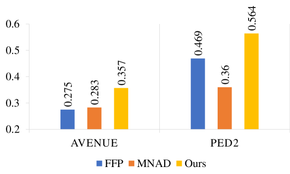
Figure 4: Following the work of Liu et al. [22], we compare our work with FFP [22] and MNAD [34] by calculating the score gap between normal frames and abnormal frames on CUHK Avenue [24] and UCSD Ped2 [30]. The gap is obtained by averaging the scores of normal frames and those of abnormal frames and subtracting the two values. A higher gap represents a higher capacity for discriminating normal and abnormal frames.

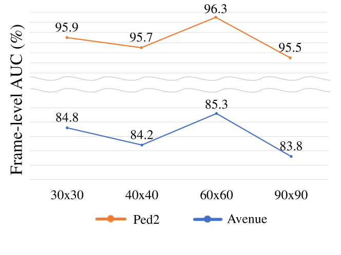
Figure 5: Results of ablation studies on patch size.

Running time. Our model boasts an astonishing speed of 195 frames per second (FPS). This rate is computed using UCSD Ped2 [30] test set with a single Nvidia GeForce RTX 3090 GPU. We obtain this by averaging the entire time consumed in both frame generation and anomaly prediction. To our knowledge, it is far faster than any other previous works. We show a fair comparison with other networks in Table 1. We re-implemented networks that distributed official codes in public on the same device and environment used for our network. The FPS for these is marked with $\dagger$ in the table. We copied the figures mentioned in each paper for methods without publicly distributed codes. Note that our work is nearly 30 % faster than the second-fastest ones [55, 25]. Moreover, we computed the number of trainable parameters as proof of 195 FPS. Its value for our model is 2.15 M whereas it is 15.65 M for MNAD[34] with 67 FPS and 14.53 M for FFP[22] with 25 FPS. Our network is remarkably cheaper in computation than the compared methods.

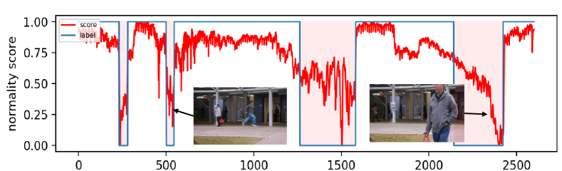
(a) CUHK Avenue

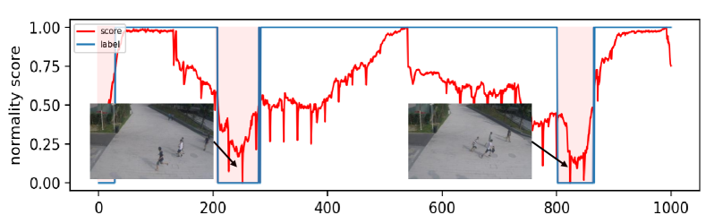
(b) ShanghaiTech

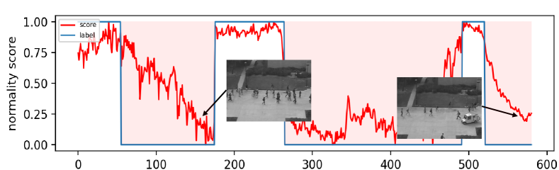
(c) UCSD Ped2

Figure 6: Score plot from evaluation. The red and blue lines denote $S_{t}$ and labels, respectively. Labels are 0 when frames are abnormal. (A) is obtained from Avenue [24]. Running, throwing a bag, and moving in the wrong direction are well detected. (B) is obtained from ShanghaiTech [28]. Chasing and running are detected as anomalies. (C) is obtained from Ped2 [30] where the captured anomalies are bicycles and a car.

Ablation studies on patch size. Fig. 5 shows the result of ablation experiments that we conducted on the Avenue [24] and Ped2 [30] to observe the effect of the patch size. The patch size determines the smallest unit to be focused on by the AE. In all experiments of these ablation studies, only the size of the patch is changed between $30\times 30$, $40\times 40$, $60\times 60$, and $90\times 90$, while the frame resolution remains fixed at $240\times 360$. It means that a comparably small region is captured in a $\mathbf{C_{f}}$ with the size of $30\times 30$, and a large region is captured in a $\mathbf{C_{f}}$ with the size of $90\times 90$. Our network shows the lowest accuracy when the patch size is $90\times 90$, which is more than 10 percent of the frame size. When the patch is considerably large, the model focuses on larger movements than smaller ones. Abnormal conditions usually occur in small parts, hence, lower performance is observed in this case.

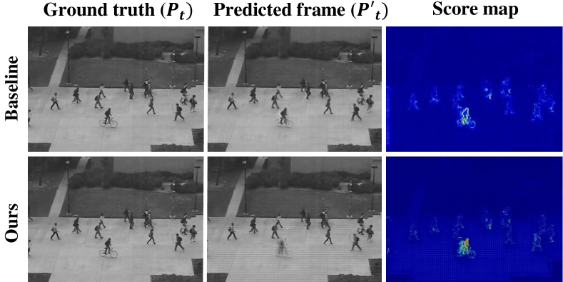
(a) UCSD Ped2

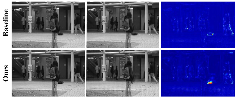
(b) CUHK Avenue

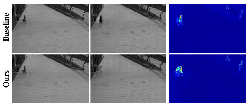
(c) ShanghaiTech

Figure 7: Examples of predicted frames and difference maps compared to our baseline. Best viewed in color.

Qualitative results. We demonstrate the frame-level detecting performance of our model in Fig. 6. From the figure, it can be observed that $S_{t}$ rapidly decreases when anomalies appear in the frames. Once the abnormal objects disappear, $S_{t}$ increases immediately.
Furthermore, the pixel-level detecting capacity is observed in Fig. 7. We present examples of predicted frames and the corresponding difference maps. Additionally, we emphasize the results by comparing each sample with those of our baseline model. In the example of Ped2 [30], the bicycle is the annotated anomaly, which is an unseen appearance. In Avenue [24] and ShanghaiTech [28], the annotated anomalies relate to motion: a man throwing a bag and a running person. The outputs generated by our model trained with the patch anomaly generation phase are significantly much blurrier than those of the baseline, validating the effectiveness of our transformation phase. Note that our model nearly erased the bag and the person in the examples of Avenue [24] and ShanghaiTech [28]. This proves that our model does not simply infer abnormal objects by copying from the inputs, which is what the baseline model does. Moreover, for the ShanghaiTech dataset [28], the difference map of our model shows a distinction in a larger region compared to that of the baseline. We observe that our model did not accept the motion in the input; it attempted to predict the trajectory of the runner as it as per the training. However, the baseline model generated a moderate copy of the input based on the given trajectory.

5 Conclusion and Future Work

In this paper, we proposed a prediction network for video anomaly detection combined with a patch anomaly generation phase. We designed a light-weight AE model to learn the common spatio-temporal features of normal frames. The proposed method generated transformed frame cuboids as inputs, by applying SRT or TMT to a random patch cuboid within the frame cuboid. Our model was encouraged to pay attention to the appearance and motion patterns of normal scenes. In addition, we discussed the impact of the patch anomaly generation by conducting ablation studies. Furthermore, the proposed method achieved competitive performance on three benchmark datasets and performed at a very high speed, which is as important as the detection capacity in anomaly detection.
Through the experimental results, we also have shown that our network is able to localize the anomalies. Since detecting temporal-wise anomalies is the most essential part and there is an inconsistency issue in pixel-level AUC evaluation [37], we only considered the frame-level detection. With the newly proposed TBDR and RBDR metrics [36], our future work will be verifying the fast localizing capability of our network.

References

- [1] Davide Abati, Angelo Porrello, Simone Calderara, and Rita Cucchiara. Latent space autoregression for novelty detection. In Proceedings of the IEEE/CVF Conference on Computer Vision and Pattern Recognition (CVPR), June 2019.
- [2] Ruichu Cai, Hao Zhang, Wen Liu, Shenghua Gao, and Zhifeng Hao. Appearance-motion memory consistency network for video anomaly detection. In Proceedings of the AAAI Conference on Artificial Intelligence, volume 35, pages 938–946, 2021.
- [3] Varun Chandola, Arindam Banerjee, and Vipin Kumar. Anomaly detection: A survey. ACM Comput. Surv., 41(3), July 2009.
- [4] Yunpeng Chang, Zhigang Tu, Wei Xie, and Junsong Yuan. Clustering driven deep autoencoder for video anomaly detection. In European Conference on Computer Vision, pages 329–345. Springer, 2020.
- [5] MyeongAh Cho, Taeoh Kim, Ig-Jae Kim, and Sangyoun Lee. Unsupervised video anomaly detection via normalizing flows with implicit latent features. arXiv preprint arXiv:2010.07524, 2020.
- [6] Yong Shean Chong and Yong Haur Tay. Abnormal event detection in videos using spatiotemporal autoencoder. In International symposium on neural networks, pages 189–196. Springer, 2017.
- [7] Terrance DeVries and Graham W Taylor. Improved regularization of convolutional neural networks with cutout. arXiv preprint arXiv:1708.04552, 2017.
- [8] Yaxiang Fan, Gongjian Wen, Deren Li, Shaohua Qiu, Martin D Levine, and Fei Xiao. Video anomaly detection and localization via gaussian mixture fully convolutional variational autoencoder. Computer Vision and Image Understanding, 195:102920, 2020.
- [9] Mariana-Iuliana Georgescu, Antonio Barbalau, Radu Tudor Ionescu, Fahad Shahbaz Khan, Marius Popescu, and Mubarak Shah. AED-SSMTL. https://github.com/lilygeorgescu/AED-SSMTL, 2021.
- [10] Mariana-Iuliana Georgescu, Antonio Barbalau, Radu Tudor Ionescu, Fahad Shahbaz Khan, Marius Popescu, and Mubarak Shah. Anomaly detection in video via self-supervised and multi-task learning. In Proceedings of the IEEE/CVF Conference on Computer Vision and Pattern Recognition, pages 12742–12752, 2021.
- [11] Mariana Iuliana Georgescu, Radu Ionescu, Fahad Shahbaz Khan, Marius Popescu, and Mubarak Shah. A background-agnostic framework with adversarial training for abnormal event detection in video. IEEE Transactions on Pattern Analysis and Machine Intelligence, page 1–1, 2021.
- [12] Dong Gong, Lingqiao Liu, Vuong Le, Budhaditya Saha, Moussa Reda Mansour, Svetha Venkatesh, and Anton van den Hengel. Memorizing normality to detect anomaly: Memory-augmented deep autoencoder for unsupervised anomaly detection. In Proceedings of the IEEE/CVF International Conference on Computer Vision, pages 1705–1714, 2019.
- [13] Mahmudul Hasan, Jonghyun Choi, Jan Neumann, Amit K Roy-Chowdhury, and Larry S Davis. Learning temporal regularity in video sequences. In Proceedings of the IEEE conference on computer vision and pattern recognition, pages 733–742, 2016.
- [14] Geoffrey E Hinton and Ruslan R Salakhutdinov. Reducing the dimensionality of data with neural networks. science, 313(5786):504–507, 2006.
- [15] Radu Tudor Ionescu, Fahad Shahbaz Khan, Mariana-Iuliana Georgescu, and Ling Shao. Object-centric auto-encoders and dummy anomalies for abnormal event detection in video. In Proceedings of the IEEE/CVF Conference on Computer Vision and Pattern Recognition, pages 7842–7851, 2019.
- [16] Jingwei Ji, Kaidi Cao, and Juan Carlos Niebles. Learning temporal action proposals with fewer labels. In Proceedings of the IEEE/CVF International Conference on Computer Vision, pages 7073–7082, 2019.
- [17] Abhishek Joshi and Vinay P Namboodiri. Unsupervised synthesis of anomalies in videos: Transforming the normal. In 2019 International Joint Conference on Neural Networks (IJCNN), pages 1–8. IEEE, 2019.
- [18] Diederik P Kingma and Jimmy Ba. Adam: A method for stochastic optimization. arXiv preprint arXiv:1412.6980, 2014.
- [19] Nikos Komodakis and Spyros Gidaris. Unsupervised representation learning by predicting image rotations. In International Conference on Learning Representations (ICLR), Vancouver, Canada, Apr. 2018.
- [20] Alex Krizhevsky, Ilya Sutskever, and Geoffrey E Hinton. Imagenet classification with deep convolutional neural networks. Advances in neural information processing systems, 25:1097–1105, 2012.
- [21] Sangmin Lee, Hak Gu Kim, and Yong Man Ro. Stan: Spatio-temporal adversarial networks for abnormal event detection. In 2018 IEEE international conference on acoustics, speech and signal processing (ICASSP), pages 1323–1327. IEEE, 2018.
- [22] Wen Liu, Weixin Luo, Dongze Lian, and Shenghua Gao. Future frame prediction for anomaly detection – a new baseline. In Proceedings of the IEEE Conference on Computer Vision and Pattern Recognition (CVPR), June 2018.
- [23] Ilya Loshchilov and Frank Hutter. Sgdr: Stochastic gradient descent with warm restarts. arXiv preprint arXiv:1608.03983, 2016.
- [24] Cewu Lu, Jianping Shi, and Jiaya Jia. Abnormal event detection at 150 fps in matlab. In Proceedings of the IEEE international conference on computer vision, pages 2720–2727, 2013.
- [25] Cewu Lu, Jianping Shi, and Jiaya Jia. Abnormal event detection at 150 fps in matlab. In Proceedings of the IEEE International Conference on Computer Vision (ICCV), December 2013.
- [26] Yiwei Lu, K Mahesh Kumar, Seyed shahabeddin Nabavi, and Yang Wang. Future frame prediction using convolutional vrnn for anomaly detection. In 2019 16th IEEE International Conference on Advanced Video and Signal Based Surveillance (AVSS), pages 1–8. IEEE, 2019.
- [27] Yiwei Lu, Frank Yu, Mahesh Kumar Krishna Reddy, and Yang Wang. Few-shot scene-adaptive anomaly detection. In European Conference on Computer Vision, pages 125–141. Springer, 2020.
- [28] Weixin Luo, Wen Liu, and Shenghua Gao. A revisit of sparse coding based anomaly detection in stacked rnn framework. In Proceedings of the IEEE International Conference on Computer Vision, pages 341–349, 2017.
- [29] Andrew L Maas, Awni Y Hannun, and Andrew Y Ng. Rectifier nonlinearities improve neural network acoustic models. In Proc. icml, volume 30, page 3. Citeseer, 2013.
- [30] Vijay Mahadevan, Weixin Li, Viral Bhalodia, and Nuno Vasconcelos. Anomaly detection in crowded scenes. In 2010 IEEE Computer Society Conference on Computer Vision and Pattern Recognition, pages 1975–1981. IEEE, 2010.
- [31] Vinod Nair and Geoffrey E Hinton. Rectified linear units improve restricted boltzmann machines. In Icml, 2010.
- [32] Trong-Nguyen Nguyen and Jean Meunier. Anomaly detection in video sequence with appearance-motion correspondence. In Proceedings of the IEEE/CVF International Conference on Computer Vision (ICCV), October 2019.
- [33] Trong Nguyen Nguyen and Jean Meunier. Hybrid deep network for anomaly detection. arXiv preprint arXiv:1908.06347, 2019.
- [34] Hyunjong Park, Jongyoun Noh, and Bumsub Ham. Learning memory-guided normality for anomaly detection. In Proceedings of the IEEE/CVF Conference on Computer Vision and Pattern Recognition, pages 14372–14381, 2020.
- [35] Adam Paszke, Sam Gross, Soumith Chintala, Gregory Chanan, Edward Yang, Zachary DeVito, Zeming Lin, Alban Desmaison, Luca Antiga, and Adam Lerer. Automatic differentiation in pytorch. 2017.
- [36] Bharathkumar Ramachandra and Michael Jones. Street scene: A new dataset and evaluation protocol for video anomaly detection. In Proceedings of the IEEE/CVF Winter Conference on Applications of Computer Vision (WACV), March 2020.
- [37] Bharathkumar Ramachandra, Michael Jones, and Ranga Raju Vatsavai. A survey of single-scene video anomaly detection. IEEE Transactions on Pattern Analysis and Machine Intelligence, pages 1–1, 2020.
- [38] Mahdyar Ravanbakhsh, Moin Nabi, Hossein Mousavi, Enver Sangineto, and Nicu Sebe. Plug-and-play cnn for crowd motion analysis: An application in abnormal event detection. In 2018 IEEE Winter Conference on Applications of Computer Vision (WACV), pages 1689–1698. IEEE, 2018.
- [39] Mahdyar Ravanbakhsh, Moin Nabi, Enver Sangineto, Lucio Marcenaro, Carlo Regazzoni, and Nicu Sebe. Abnormal event detection in videos using generative adversarial nets. In 2017 IEEE International Conference on Image Processing (ICIP), pages 1577–1581. IEEE, 2017.
- [40] Mahdyar Ravanbakhsh, Enver Sangineto, Moin Nabi, and Nicu Sebe. Training adversarial discriminators for cross-channel abnormal event detection in crowds. In 2019 IEEE Winter Conference on Applications of Computer Vision (WACV), pages 1896–1904. IEEE, 2019.
- [41] Olaf Ronneberger, Philipp Fischer, and Thomas Brox. U-net: Convolutional networks for biomedical image segmentation. In International Conference on Medical image computing and computer-assisted intervention, pages 234–241. Springer, 2015.
- [42] Waqas Sultani, Chen Chen, and Mubarak Shah. Real-world anomaly detection in surveillance videos. In Proceedings of the IEEE conference on computer vision and pattern recognition, pages 6479–6488, 2018.
- [43] Yao Tang, Lin Zhao, Shanshan Zhang, Chen Gong, Guangyu Li, and Jian Yang. Integrating prediction and reconstruction for anomaly detection. Pattern Recognition Letters, 129:123–130, 2020.
- [44] Du Tran, Lubomir Bourdev, Rob Fergus, Lorenzo Torresani, and Manohar Paluri. Learning spatiotemporal features with 3d convolutional networks. In Proceedings of the IEEE international conference on computer vision, pages 4489–4497, 2015.
- [45] Zhou Wang, Alan C Bovik, Hamid R Sheikh, and Eero P Simoncelli. Image quality assessment: from error visibility to structural similarity. IEEE transactions on image processing, 13(4):600–612, 2004.
- [46] Ziming Wang, Yuexian Zou, and Zeming Zhang. Cluster attention contrast for video anomaly detection. In Proceedings of the 28th ACM International Conference on Multimedia, pages 2463–2471, 2020.
- [47] Dan Xu, Yan Yan, Elisa Ricci, and Nicu Sebe. Detecting anomalous events in videos by learning deep representations of appearance and motion. Computer Vision and Image Understanding, 156:117–127, 2017.
- [48] Muchao Ye, Xiaojiang Peng, Weihao Gan, Wei Wu, and Yu Qiao. Anopcn: Video anomaly detection via deep predictive coding network. In Proceedings of the 27th ACM International Conference on Multimedia, pages 1805–1813, 2019.
- [49] Guang Yu, Siqi Wang, Zhiping Cai, En Zhu, Chuanfu Xu, Jianping Yin, and Marius Kloft. Cloze test helps: Effective video anomaly detection via learning to complete video events. In Proceedings of the 28th ACM International Conference on Multimedia, pages 583–591, 2020.
- [50] Sangdoo Yun, Dongyoon Han, Seong Joon Oh, Sanghyuk Chun, Junsuk Choe, and Youngjoon Yoo. Cutmix: Regularization strategy to train strong classifiers with localizable features. In Proceedings of the IEEE/CVF International Conference on Computer Vision, pages 6023–6032, 2019.
- [51] Muhammad Zaigham Zaheer, Jin-ha Lee, Marcella Astrid, and Seung-Ik Lee. Old is gold: Redefining the adversarially learned one-class classifier training paradigm. In Proceedings of the IEEE/CVF Conference on Computer Vision and Pattern Recognition, pages 14183–14193, 2020.
- [52] Hongyi Zhang, Moustapha Cisse, Yann N Dauphin, and David Lopez-Paz. mixup: Beyond empirical risk minimization. arXiv preprint arXiv:1710.09412, 2017.
- [53] Hang Zhao, Orazio Gallo, Iuri Frosio, and Jan Kautz. Loss functions for image restoration with neural networks. IEEE Transactions on computational imaging, 3(1):47–57, 2016.
- [54] Yiru Zhao, Bing Deng, Chen Shen, Yao Liu, Hongtao Lu, and Xian-Sheng Hua. Spatio-temporal autoencoder for video anomaly detection. In Proceedings of the 25th ACM international conference on Multimedia, pages 1933–1941, 2017.
- [55] Jia-Xing Zhong, Nannan Li, Weijie Kong, Shan Liu, Thomas H Li, and Ge Li. Graph convolutional label noise cleaner: Train a plug-and-play action classifier for anomaly detection. In Proceedings of the IEEE/CVF Conference on Computer Vision and Pattern Recognition, pages 1237–1246, 2019.