Ada-BKB: Scalable Gaussian Process Optimization on Continuous Domains by Adaptive Discretization

Abstract

Gaussian process optimization is a successful class of algorithms(e.g. GP-UCB) to optimize a black-box function through sequential evaluations. However, for functions with continuous domains, Gaussian process optimization has to rely on either a fixed discretization of the space, or the solution of a non-convex optimization subproblem at each evaluation. The first approach can negatively affect performance, while the second approach requires a heavy computational burden. A third option, only recently theoretically studied, is to adaptively discretize the function domain. Even though this approach avoids the extra non-convex optimization costs, the overall computational complexity is still prohibitive. An algorithm such as GP-UCB has a runtime of $O(T^{4})$, where $T$ is the number of iterations. In this paper, we introduce Ada-BKB (Adaptive Budgeted Kernelized Bandit), a no-regret Gaussian process optimization algorithm for functions on continuous domains, that provably runs in $O(T^{2}d_{\text{eff}}^{2})$, where $d_{\text{eff}}$ is the effective dimension of the explored space, and which is typically much smaller than $T$. We corroborate our theoretical findings with experiments on synthetic non-convex functions and on the real-world problem of hyper-parameter optimization, confirming the good practical performances of the proposed approach.

1 INTRODUCTION

The maximization of a function given only finite, possibly noisy, evaluations is a key and common problem in applied sciences and engineering. Approaches to this problem range from genetic algorithms (Whitley,, 1994) to zero-th order methods (Nesterov and Spokoiny,, 2017). Here, we take the perspective of bandit optimization, where indeed a number of approaches have been proposed and studied: for example Thompson sampling, or the upper confidence bound algorithm (UCB), see (Lattimore and Szepesvári,, 2020) and references therein. Relevant to our study is a whole line of work developing the basic UCB idea, considering in particular kernels (kernel-UCB) (Kung,, 2014) or Gaussian processes (GP-UCB) (Rasmussen,, 2003). In the basic UCB algorithm, the function domain is typically assumed to be discrete (or discretized) and an upper bound to the function of interest is iteratively computed and maximized. This approach is sound and amenable to a rigorous theoretical analysis in terms of regret bounds. Considering Gaussian processes/kernels, it is possible to extend the applicability of UCB while preserving the nice theoretical properties (Kung,, 2014; Rasmussen,, 2003). However, this is at the expenses of computational efficiency. Indeed, a number of recent works has focused on scaling UCB with kernels/GP by taking advantage of randomized approximations based on random features (Mutnỳ and Krause,, 2019) and Nystrom/inducing points methods (Calandriello et al.,, 2020, 2019), or by performing a smart candidate selection strategy (Calandriello et al.,, 2022). These studied solutions show that improved efficiency can be achieved without degrading the regrets guarantees. The other line of work relevant to our study focuses on how to tackle functions defined on continuous domains. In particular, we consider optimistic optimization, introduced in (Munos,, 2011) and developed in a number of subsequent works, see (Valko et al., 2013a, ; Kleinberg et al.,, 2013; Bubeck et al.,, 2011; Wang et al.,, 2014; Shekhar and Javidi,, 2018; Salgia et al.,, 2020; Kleinberg et al.,, 2008). The basic idea is to iteratively build discretizations in a coarse to fine manner. This approach, related to Monte Carlo tree search, can be analyzed theoretically to derive rigorous regrets guarantees (Munos,, 2014). In this paper we propose and analyze a novel and efficient approach called Ada-BKB, that combines ideas from optimistic optimization and UCB with kernels. A first attempt in this direction has been done in (Shekhar and Javidi,, 2018; Salgia et al.,, 2020). However, the corresponding computational costs are prohibitive since exact (kernel) UCB computations are performed. So, we take advantage of the latest advances on scalable kernel UCB and adapt optimistic optimization techniques to derive a provably accurate and efficient algorithm. Our main theoretical contribution is the derivation of sharp regret guarantees, that shows that Ada-BKB is as accurate as an exact UCB with kernels, with much smaller computational costs. We provided an efficient implementation of Ada-BKB which uses techniques such as pruning and early stopping. We investigate empirically its performance both in numerical simulations and in a hyper-parameter tuning task. The obtained results confirm that Ada-BKB is a scalable and accurate algorithm for efficient bandit optimization on continuous domains. The rest of the paper is organized as follows. In Section 2, we describe the problem setting and in Section 3, we describe the algorithm we propose. In Section 4 and 5 we present our empirical and theoretical results. In Section 6 we discuss some final remarks.

2 PROBLEM SETUP

Let $(X,d)$ be a compact metric space, for example $X=[0,1]^{p}\subseteq\mathbb{R}^{p}$. Let $f:X\rightarrow\mathbb{R}$ be a continuous function and consider the problem of finding

$$x^{*}\in\operatornamewithlimits{arg\,max}\limits_{x\in X}f(x).$$

We consider a setting where only noisy function evaluations $y_{t}=f(x_{t})+\epsilon_{t}$ are accessible. Here, $\epsilon_{t}$ is $\xi$-sub Gaussian noise. This problem is relevant in black-box or zero-th order optimization (Nesterov,, 2014), as well as in muti-armed bandits (Lattimore and Szepesvári,, 2020). In this latter context, the function $f$ is also called the reward function and $X$ the arms set. Given $T\in\mathbb{N}$, the goal is to derive a sequence $x_{1},\cdots,x_{T}\in X$, with small cumulative regret,

$$R_{T}=\sum_{t=1}^{T}(f(x^{*})-f(x_{t})).$$

This can be contrasted to considering the simple regret $S_{T}=f(x^{*})-f(x_{T})$ as typically done in optimization. The regret considers the errors accumulated by the whole sequence rather than just the last iteration. The sequence $(x_{t})_{t}$ is computed iteratively. At each iteration $t$, an element $x_{t}\in X$ is selected and a corresponding noisy function value $y_{t}$ made available. The selection strategy, also called a policy, is based on all the function values obtained in previous iterations. In the following we assume $f$ to belong to a reproducing kernel Hilbert space (RKHS). The latter is a Hilbert space of $(\mathcal{H},\left\langle{\cdot},{\cdot}\right\rangle,\|\cdot\|)$ of functions from $X$ to $\mathbb{R}$, with associated a function $k:X\times X\to\mathbb{R}$, called reproducing kernel or kernel, such that for all $x\in X$ and $f^{\prime}\in\mathcal{H}$,

$$k(x,\cdot)\in\mathcal{H},\qquad\text{and}\qquad f^{\prime}(x)=\left\langle{f^{\prime}},{k(x,\cdot)}\right\rangle.$$

We assume that $k(x,x)\leq\kappa^{2}$ for all $x\in X$ and $\kappa\geq 1$. We let $d_{k}:X\times X\rightarrow[0,\infty)$ be the distance in the RKHS $\mathcal{H}$ defined as $d_{k}(x,x^{\prime})=\left\lVert{k(x,\cdot)-k(x^{\prime},\cdot)}\right\rVert=\sqrt{k(x,x)+k(x^{\prime},x^{\prime})-2k(x,x^{\prime})}$ with $x,x^{\prime}\in X$. Further, we consider kernels for which the following assumptions hold.

Assumption 1.

There exists a non-decresing function $g:[0,\infty)\to[0,\infty)$ such that $g(0)=0$ and for all $x,x^{\prime}\in X$

$$d_{k}(x,x^{\prime})\leq g(d(x,x^{\prime})).$$ (1)

Assumption 2.

Let $g$ be the non-decreasing function indicated in Assumption 1. There exist $\delta_{k}>0$, $\alpha\in(0,1]$, and $C^{\prime}_{k},C_{k}>0$ such that

$$(\forall r\leq\delta_{k})\qquad C_{k}r^{\alpha}\leq g(r)\leq C^{\prime}_{k}r^{\alpha}$$ (2)

It is easy to see that, the above condition is satisfied, for example, for the Gaussian kernel $k(x_{1},x_{2})=e^{-\frac{\left\lVert{x_{1}-x_{2}}\right\rVert^{2}}{l}}$ with $\alpha=1$ and suitable constants $\delta_{k},C_{k},C_{k}^{\prime}$, for $g(r)=\sqrt{\frac{2}{l}}r$.

3 ALGORITHM

The new algorithm we propose combines ideas from AdaGP-UCB (Shekhar and Javidi,, 2018) and BKB (Calandriello et al.,, 2019) (a scalable implementation of GP-UCB/KernelUCB (Srinivas et al.,, 2010; Valko et al., 2013b, )). We begin recalling the ideas behind GP-UCB and BKB.

From kernel bandits to budgeted kernel bandits.

The basic idea in GP-UCB/KernelUCB is to derive an upper estimate $f_{t}$ of $f$ at each step, and then select the new point $x_{t+1}$ maximizing such an estimate. The upper estimate is defined using a reproducing kernel $k:X\times X\rightarrow\mathbb{R}$. Let $(x_{1},y_{1}),\dots,(x_{t},y_{t})$ be the sequence of evaluations points and noisy evaluation values up-to the $t$-th iteration. Let $K_{t}\in\mathbb{R}^{t\times t}$ be the matrix with entries $(K_{t})_{ij}=k(x_{i},x_{j})$, for $i,j=1,\dots,t$, denote $k_{t}(x)=(k(x,x_{1}),\dots,k(x,x_{t}))\in\mathbb{R}^{t}$ and $Y_{t}=(y_{1},\dots,y_{t})\in\mathbb{R}^{t}$. For $\lambda>0$, let

$$\mu_{t}(x) =k_{t}(x)^{\top}(K_{t}+\lambda I)^{-1}Y_{t}$$ (3)

$$\sigma_{t}(x)^{2} =k(x,x)-k_{t}(x)^{\top}(K_{t}+\lambda I)^{-1}k_{t}(x).$$

For $\beta_{t}>0$, the upper estimate of $f$, known as upper confidence bound (UCB), is defined as

$$f_{t}(x)=\mu_{t}(x)+\beta_{t}\sigma_{t}(x).$$

Note that $\lambda$ and $\beta_{t}$ are parameters that need to be specified. The quantities $\mu_{t},\sigma_{t}$ can be seen as a kernel ridge regression estimate and a suitable confidence bound, respectively. Also, they have a natural Bayesian interpretation in terms of mean and variance of the posterior induced by a Gaussian Process, hence the name GP-UCB (Srinivas et al.,, 2010). KernelUCB/GP-UCB have favorable regret guarantees (Valko et al., 2013b, ; Srinivas et al.,, 2012), but computational requirements that prevent scaling to large data-sets. BKB (Calandriello et al.,, 2019) tackles this issues considering a Nyström-based approximation (Drineas et al.,, 2005). Let $X_{t}=(x_{1},\dots,x_{t})\in\mathbb{R}^{t\times p}$ be the collection of evaluation points up-to iteration $t$ and $S_{t}\subseteq X_{t}$ a subset of cardinality $m\leq t$. Let $K_{S_{t}}\in\mathbb{R}^{m\times m}$ such that $(K_{S_{t}})_{ij}=k(x_{i},x_{j})$ with $x_{i},x_{j}\in S_{t}$, and $k_{S_{t}}(x)\in\mathbb{R}^{m}$ such that $(k_{S_{t}}(x))_{i}=k(x,x_{i})$ with $x_{i}\in S_{t}$. Let $\widetilde{k}:X\times X\rightarrow\mathbb{R}$ be the approximate Nyström kernel defined as

$$\widetilde{k}(x,x^{\prime})=k_{S_{t}}(x)^{\top}K_{S_{t}}^{\dagger}k_{S_{t}}(x^{\prime}).$$ (4)

Let $\widetilde{K}_{S_{t}}\in\mathbb{R}^{t\times t}$ such that $(\widetilde{K}_{S_{t}})_{ij}=\widetilde{k}(x_{i},x_{j})$ with $x_{i},x_{j}\in X_{t}$, and $\widetilde{k}_{S_{t}}(x)\in\mathbb{R}^{t}$ such that $(\widetilde{k}_{S_{t}}(x))_{i}=\widetilde{k}(x,x_{i})$ with $x_{i}\in X_{t}$.

For $\lambda>0$, let

$$\widetilde{\mu}_{t}(x_{i}) =\widetilde{k}_{S_{t}}(x_{i})^{\top}(\widetilde{K}_{S_{t}}+\lambda I)^{-1}Y_{t}$$ (5)

$$\widetilde{\sigma}^{2}_{t}(x_{i}) =\frac{1}{\lambda}(k(x_{i},x_{i})-\widetilde{k}_{S_{t}}(x_{i})^{\top}(\widetilde{K}_{S_{t}}+\lambda I)^{-1}\widetilde{k}_{S_{t}}(x_{i}))$$

and, for $\beta_{t}>0$

$$\widetilde{f}_{t}(x)=\widetilde{\mu}_{t}(x)+\beta_{t}\widetilde{\sigma}_{t}(x).$$ (6)

BKB uses the above approximate estimate and select at each iterations the points in $S_{t}$ proportionally to their variance at the previous iterate $\widetilde{\sigma}_{t-1}^{2}(x_{i})$ (Calandriello et al.,, 2019). This sampling strategy guarantees that, for the proper values of $\beta_{t}$, $|S_{t}|\leq O(d_{\text{eff}}(t))$ where $\widetilde{X}_{t}$ is the set of explored points until function evaluation $t$ and $d_{\text{eff}}$ is the effective dimension, a quantity typically much lower than $t$ and defined as

$$d_{\text{eff}}(t)=\sum\limits_{t=1}^{T}\sigma_{t}^{2}(x_{t}).$$ (7)

where with $x_{t}$ is the point evaluated at time $t$. To maximize the upper estimate ($f_{t}$ for KernelUCB/GP-UCB and $\widetilde{f}_{t}$ for BKB) these algorithms rely on the assumption that the arms set $X$ is discrete. In practice, when $X$ is continuous, a fixed discretization is considered. In the next section we discuss how the latter can be computed adaptively and introduce some necessary concepts and assumptions.

Partition Trees.

Key for adaptive discretization is a family of partitions called partition trees. Following (Shekhar and Javidi,, 2018), the notion of partition tree for metric spaces is formalized by the following definition.

Definition 1.

Let $(X_{h})_{h\in\mathbb{N}}$ be families of subsets of $X$, with $X_{0}=X$. For each $h\in\mathbb{N}$ (called depth), the family of subsets $X_{h}$ has cardinality $N^{h}$ with $N\in\mathbb{N}$. The elements of $X_{h}$ are denoted by $X_{h,i}$ and called cells. Each cell $X_{h,i}$ is identified by the point $x_{h,i}\in X_{h,i}$ (called centroid) such that

$$X_{h,i}=\{x\in X:d(x,x_{h,i})\leq d(x,x_{h,j})\quad\forall j\neq i\}.$$

Further, for all $h\in\mathbb{N}$ and $i=1,\dots,N^{h}$,

$$X_{h,i}=\cup_{j=N(i-1)+1}^{Ni}X_{h+1,j}.$$

The cells $(X_{h+1,j})_{j}$ are called children of $X_{h,i}$, and $X_{h,i}$ is called parent of $(X_{h+1,j})_{j}$.

Note that each cell $X_{h,i}$ identifies a node in the tree denoted by the index $(h,i)$. To describe the above parent/children relationship we define the following function on indexes. Let $(0,1)$ be the index of the root cell $X_{0,1}=X$, we denote with $p$ that function that given the index of a cell $(h+1,j)$ returns the index of its parent $(h,i)$, and with $c$ that function that given the index of a cell $(h,i)$ returns the indexes of its children $\{(h+1,N(i-1)+1),\dots,(h+1,Ni)\}$. In the following we refers to $p$ and $c$ as parent function and children function.

Partition growth and maximum local reward variation.

We make the following assumption which formalizes the idea that the cell size decreases with depth.

Assumption 3.

Let $B(x,r,d)$ be a $d$-ball with radius $r$ and centered in $x$, we assume that there exist $\rho\in(0,1)$ and $0<v_{2}\leq 1\leq v_{1}$ such that for $h\geq 0$ and all $i=1,\dots,N^{h}$

$$B(x_{h,i},v_{2}\rho^{h},d)\subset X_{h,i}\subset B(x_{h,i},v_{1}\rho^{h},d)$$

Knowing that $f\in\mathcal{H}$, from the above assumption and Assumption 1 we can derive the following upper bound on the maximum variation of $f$ in the cells $(X_{h,i})_{i}$ at each depth $h$.

Lemma 1.

Under Assumptions 1 and 3, let $f\in\mathcal{H}$ and let $F=\|f\|$. Then, for all $h\geq 0$ and for all $1\leq i\leq N^{h}$,

$$\sup\limits_{x,x^{\prime}\in X_{h,i}}|f(x)-f(x^{\prime})|\leq V_{h}$$ (8)

with $V_{h}=Fg(v_{1}\rho^{h})$

We provide the proof in Appendix B.1

3.1 Ada-BKB

We now present the new algorithm called Adaptive-BKB (Ada-BKB). Given a partition tree and a function evaluation budget $T$, the basic idea is to explore the set of arms in a coarse to fine fashion, considering a variation of BKB on the cells’ centroids of the partition tree. The algorithm is given in Algorithm 1 and we next describe its various steps.

Preliminaries: index function and leaf set.

Recalling the definition of the parent function $p$, given $x_{h,i}\in X_{h,i}$ we let $x_{p(h,i)}$ be the centroid of the parent cell. Then, we define the so called index function as

$$I_{t}(x_{h,i})=\min(\widetilde{f}_{t}(x_{h,i}),\widetilde{f}_{t}(x_{p(h,i)})+V_{h-1})+V_{h}$$ (9)

with $\widetilde{f}_{t}$ as in (6). In other terms, we compute an high probability upper bound of $f$ on $x_{h,i}$ and, adding $V_{h}$, we get an high probability upper bound over the maximum values of $f$ in the cell $X_{h,i}$.

Ada-BKB proceeds iteratively. The algorithm maintains two counters, $\tau$ which counts the total number of function evaluations and refinements (see below), and $t$ which keeps track of the number of function evaluations performed. A set of cells’ centroids $L_{\tau}$ (called the leaf set) is updated at each iteration $\tau\geq 0$. We next describe how the leaf set is used and populated recursively.

First evaluation-update steps.

The leaf set initially contains only the centroid of root cell, that is

$$L_{0}=\{x_{0,1}\}.$$

The function value is queried at $x_{0,1}$ to obtain $y_{1}=f(x_{0,1})+\varepsilon_{1}$ and the first estimates $\widetilde{\mu}_{1},\widetilde{\sigma}_{1}$ are computed. Then, given a suitable parameter $\beta_{t}$, the condition,

$${\beta_{t}}\widetilde{\sigma}_{1}(x_{0,1})\leq V_{0},$$

is checked. Initially the term $\widetilde{\sigma}_{1}(x_{0,1})$ is typically large and the condition is violated. In this case, another function value

$$y_{2}=f(x_{0,1})+\varepsilon_{2}$$

is queried to derive new estimates $\widetilde{\mu}_{2},\widetilde{\sigma}_{2}$ using all available data. Then, the condition ${\beta_{t}}\widetilde{\sigma}_{2}(x_{0,1})\leq V_{0}$ is checked again. If violated more function values $y_{t}=f(x_{0,1})+\varepsilon_{t}$ are queried, and estimates $\widetilde{\mu}_{t},\widetilde{\sigma}_{t}$ computed, until the condition ${\beta_{t}}\widetilde{\sigma}_{t}(x_{0,1})\leq V_{0}$ is satisfied . Both counters are updated i.e. $\tau=t$.

First leaf-set-expansion step.

During all the above iterations the leaf set is unchanged, so that $L_{\tau}=L_{0}$. When the condition ${\beta_{t}}\widetilde{\sigma}_{t}(x_{0,1})\leq V_{0}$ is satisfied, then the leaf set is expanded according to the following rule

$$L_{\tau+1}=(L_{\tau}\setminus\{x_{0,1}\})\cup\{x_{1,j}|1\leq j\leq N\},$$

and the counter $\tau$ is incremented by $1$. In words, the cell we just evaluated is taken off the leaf set and its children included.

Figure 1: Description of the first and second refinement procedures. The $x_{h,i}$ are the centroids contained in the leaf set while the $\bullet$ represent the centroid removed after the refinement procedure. From left to right, the initial state of the leaf set (containing only the centroid of the root cell), the first refinement and a second refinement with number of children per cell $N=2$.

Further evaluation-update steps.

The estimates $\widetilde{\mu}_{t},\widetilde{\sigma}_{t}$ are computed and used to build $I_{t}$ as in (9). Then, the cell $x_{1,i}$ in the leaf set $L_{\tau}$ maximizing the index function is selected,

$$x_{1,i}=\operatornamewithlimits{arg\,max}_{x\in L_{\tau}}I_{t}(x).$$

The condition ${\beta_{t}}\widetilde{\sigma}_{t}(x_{1,i})\leq V_{1}$ is then checked. If violated a value $y_{t+1}=f(x_{1,i})+\varepsilon_{t+1}$ is queried and then the estimates $\widetilde{\mu}_{t+1},\widetilde{\sigma}_{t+1}$and $I_{t+1}$ computed. A new cell is then selected as above

$$x_{1,i^{\prime}}=\operatornamewithlimits{arg\,max}_{x\in L_{\tau+1}}I_{t+1}(x).$$

Note that, we might obtain the same cell $i=i^{\prime}$ or a different cell $i\neq i^{\prime}$. Again the condition ${\beta_{t}}\widetilde{\sigma}_{t+1}(x_{1,i^{\prime}})\leq V_{1}$ is checked until satisfied, and this can entail querying multiple evaluations, possible at more cells.

Further leaf-set-expansion steps.

Note that, throughout the possible function evaluations the leaf set remains unchanged. Also, while we might evaluate multiple cells, at some point the condition ${\beta_{t}}\widetilde{\sigma}_{t+1}(x_{1,i^{\prime}})\leq V_{1}$ will be satisfied by a given cell. Then, indicating with $c(\cdot)$ the function which given a centroid returns the set of children of node represented by the given centroid i.e.

$$c(x_{h,i})=\{x_{h+1,j}|N(i-1)+1\leq j\leq Ni\}$$

the leaf set will be updated as follow

$$L_{\tau+1}=(L_{\tau}\setminus\{x_{h,i^{\prime}}\})\cup\text{c}(x_{h,i^{\prime}})$$

The cell $x_{h,i^{\prime}}$ we last evaluated is taken off the leaf set, its children $x_{h+1,j}$, $N(i-1)+1\leq j\leq Ni$ added, but note that also all the cells $x_{h,i}$, $i\neq i^{\prime}$ in the same partition as $x_{h,i^{\prime}}$ are kept in the leaf set. Moreover, in order to avoid the (unlikely) scenarios in which the algorithm keeps refining indefinitely without evaluating the function, a maximum depth threshold $h_{\text{max}}$ is added.

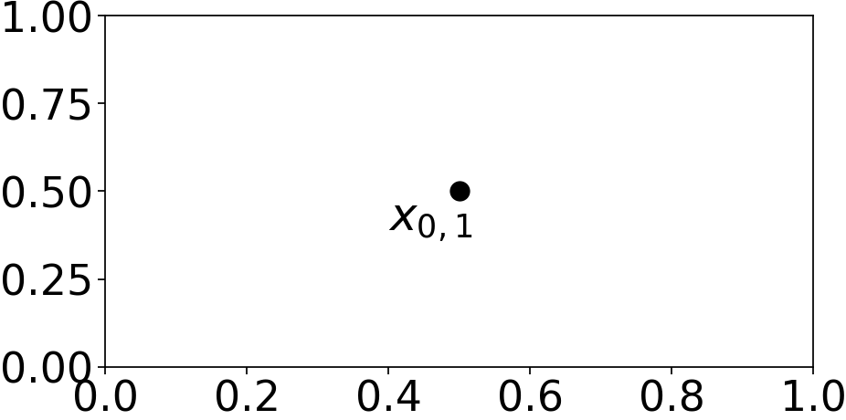
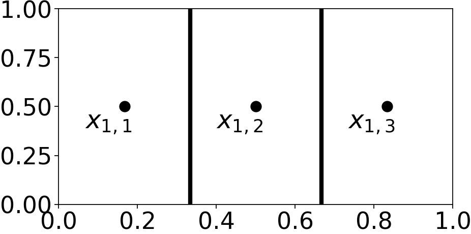
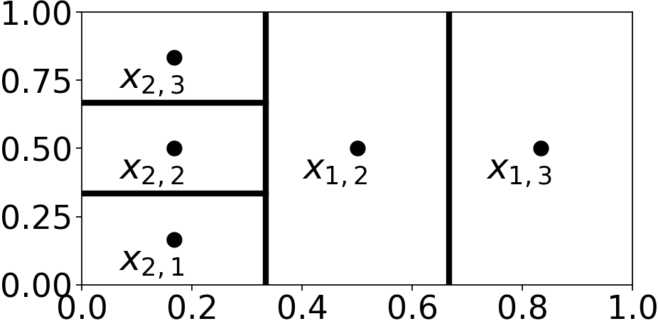
Figure 2: Consider $X=[0,1]^{2}$ and $N=3$. Here $\bullet$ denotes the centroids. The first picture (from top to bottom), represent the initialization of the algorithm where we have only the root ($X=X_{0,1}=[0,1]^{2}$); the second picture, represent the first refinement in which we split the root cell in $N=3$ cells associated to the children ($(1,1)$ has $X_{1,1}=[0,1/3]\times[0,1]$, $(1,2)$ has $X_{1,2}=[1/3,2/3]\times[0,1]$ and $(1,3)$ has $X_{1,3}=[2/3,1]\times[0,1]$). The third picture, represent the expansion of cell $(1,1)$.

Pruning rule.

One of the core differences between Ada-BKB and AdaGP-UCB is the presence of a pruning rule. This rule eliminates the cells that in high probability don’t contain a global maximizer. Let $X_{t}$ be the set of centroids observed until time $t$, and let the highest lower confidence bound (LCB) be defined as

$$l^{*}_{t}=\max\limits_{x\in X_{t}}\tilde{\mu}_{t}(x)-\tilde{\beta}_{t}\tilde{\sigma}_{t}(x)$$

After each iteration, the pruning rule erases every centroid in the leaf set $L_{\tau}$ that have their upper bound on the maximum over the cell smaller than $l^{*}_{t}$. Formally, we define a function er${}_{t}:X\rightarrow\{0,1\}$ which, given a centroid $x_{h,i}$, returns $1$ if the centroid needs to be pruned and $0$ otherwise

$$\text{er}_{t}(x_{h,i})=\begin{cases}1&\text{if}\quad\tilde{f}_{t-1}(x_{h,i})+V_{h}<l^{*}\\ 0&\text{otherwise}\end{cases}$$

Thus, the leaf set is updated as $L_{\tau+1}=L_{\tau+1}\setminus\{x_{h,i}\in L_{\tau+1}:\text{ er}(x_{h,i})>0\}$. Notice that this pruning rule doesn’t increase the computational cost since all the information used for the check must be computed previously for different reasons (as the UCB + $V_{h}$) and the best lower bound can be stored and updated after every evaluation (the informations used for the best lower bound, i.e. $\tilde{\mu}_{t}$ and $\tilde{\beta}_{t}\tilde{\sigma}_{t-1}$, are already computed for the index function). Notice that if an expansion is performed the centroids to check are just the new ones (since the model is not updated).

Moreover, this pruning rule automatically provide us an early stopping condition, infact, if after the pruning procedure the leaf set size is $0$ or $1$ and the only centroid contained in the set is $x_{h_{\text{max}},i}$, we can interrupt the execution and terminate the algorithm since every subsequent evaluation will be performed on this centroid. In practice, this procedure is very useful because it allows to limit the effects of over-expansion of the tree that would make the algorithm very time-expensive (see Section 5 and Appendix C.4).

Algorithm 1 Ada-BKB

1:Input: $T>0$, $h_{\text{max}}$, $N$, $\beta_{t}$

2:Initialize $L_{0}=\{x_{0,1}\},\tau=0,t=1$

3:while $t\leq T$ do

4:     $x_{h,i}=\operatornamewithlimits{arg\,max}\limits_{x_{i}\in L_{\tau}}I_{t}(x_{i})$

5:     if ${\beta_{t}}\widetilde{\sigma}_{t-1}(x_{h,i})\leq V_{h}$ and $h_{t}<h_{\text{max}}$ then

6:         $L_{\tau+1}=(L_{\tau}\setminus\{x_{h,i}\})\cup c(x_{h,i})$

7:     else

8:         $y_{t}=f(x_{h,i})+\epsilon_{t}$ (with $\epsilon_{t}$ noise)

9:         compute $\widetilde{\mu}_{t+1},\widetilde{\sigma}_{t+1},l^{*}_{t+1}$

10:         $L_{\tau+1}=L_{\tau}$

11:         $t=t+1$      

12:     $L_{\tau+1}=L_{\tau+1}\setminus\{x_{h,i}:\text{ er}(x_{h,i})>0\}$

13:     if $|L_{\tau+1}|==0$ or $L_{\tau+1}==\{x_{h_{\text{max}},i}\}$  then

14:         break      

15:     $\tau=\tau+1$

Note that, when performing a leaf-set-expansion step, we have yet to specify how to choose N children. Thus we consider the refinement of a cell $X_{h,i}$ is performed by dividing it equally in $N$ parts along its longest side. This is a common method which allows to get a partition tree defined as in Definition 1 satisfying also Assumption 3 as shown in (Shekhar and Javidi,, 2018; Bubeck et al.,, 2011; Salgia et al.,, 2020)

4 MAIN RESULTS

In this section we present the two main theorems of the paper. Theorem 1 shows that the regret bounds for Ada-BKB are the same as those of exact GP-UCB, while in Theorem 2 we prove that the computational cost of Ada-BKB is smaller that the one of other adaptive methods. Altogether, our results show that, thanks to the use of sketching, Ada-BKB a fast adaptive method achieving state-of-the-art regret bounds.

4.1 Regret Analysis

We next present the first main contribution of the paper on the cumulative regret, for a given function in the considered reproducing kernel Hilbert space. We recall that we have access to noisy function evaluations $y_{t}=f(x_{t})+\epsilon_{t}$, where $\epsilon_{t}$ is $\xi$-sub Gaussian.

Theorem 1 (Regret Bounds).

Let $f\in\mathcal{H}$, and let $F=\|f\|$. Let $\delta\in(0,1)$, $\epsilon\in(0,1)$ and $\bar{\alpha}=\frac{1+\epsilon}{1-\epsilon}$. Suppose that Assumptions 1,2,3 are satisfied. Consider Ada-BKB (Alg. 1) with $N\geq 1$, $T\geq(v_{1}/\delta_{k})^{2\alpha}$, $h_{\text{max}}\geq\frac{\log(T)}{2\alpha\log(1/\rho)}$, $\lambda=\xi^{2}$, $\zeta_{t}=\bar{\alpha}\log(\kappa^{2}t)\Big{(}\sum\limits_{s=1}^{t}\widetilde{\sigma}_{t}^{2}(x_{s})\Big{)}$ and $\beta_{t}$ defined as

$${\beta}_{t}=2\lambda^{2}\sqrt{\zeta_{t}+\log(1/\delta)}+\Big{(}1+\frac{1}{\sqrt{1-\epsilon}}\Big{)}\sqrt{\lambda}F.$$ (10)

Then, with probability at least $1-\delta$,

$$R_{T}\leq\mathcal{O}(\sqrt{T}d_{\text{eff}}(T)\log(T)).$$ (11)

Moreover, if the evaluation model is $y_{t}=f(x_{t})+\eta_{t}\quad\eta_{t}\sim\mathcal{N}(0,\sigma^{2})$, the cumulative regret can be bounded as:

$$R_{T}\leq\mathcal{O}\Bigg{(}\sqrt{Td_{\text{eff}}(T)\log(T)\frac{N^{h_{\text{max}}}-1}{N-1}}\Bigg{)}.$$ (12)

The above Theorem shows that the regret bound for Ada-BKB matches exactly the regret bounds of the non-adaptive methods BKB and BBKB (Calandriello et al.,, 2020). The comparison is straightforward, since the bounds for all the methods are expressed in terms of the same quantities. AdaGP-UCB and the non-adaptive methods GP-UCB (Srinivas et al.,, 2010), TS-QFF (Mutnỳ and Krause,, 2019) have a regret of $O(\sqrt{T}\gamma_{T})$, where $\gamma_{T}$ is the mutual information gain. It is shown in (Calandriello et al.,, 2019) that $\gamma_{T}$ is of the same order of $d_{\text{eff}}(T)$, and therefore the regret bounds for Ada-BKB are better when $\sqrt{\log(T)\frac{N^{h_{\text{max}}}-1}{N-1}}\leq\sqrt{d_{\text{eff}}(T)}$. Finally, we recall that GP-ThreDS (Salgia et al.,, 2020) has a regret bound of $O(\sqrt{T\gamma_{T}}(\log T)^{2})$, namely $O(\sqrt{Td_{\text{eff}}(T)}(\log T)^{2})$ and thus in this case Ada-BKB can be advantageous if $\sqrt{\log(T)\frac{N^{h_{\text{max}}}-1}{N-1}}\leq(\log T)^{2}$. We extend the discussion in appendix D

4.2 Computational Cost Analysis

In this section we compute the total computational cost of Ada-BKB, for a specific choice of the family of partition, in the case $X=[0,1]^{p}$. The computational cost of Ada-BKB is due to the following operations: 1) the computation of $\widetilde{f}_{t}$, 2) the computation of $I_{t}(x)$ for all $x\in L_{\tau}$, 3) the discretization refinement. We bound each cost separately.

1) The cost of computing $\widetilde{f}_{t}$ is the cost of computing $\widetilde{\mu}_{t},\widetilde{\sigma}_{t}$ and $\beta_{t}$. The time complexity of computing these quantities over $T$ observations is $\mathcal{O}(Td^{2}_{\text{eff}}(T))$ (Calandriello et al.,, 2019).

2) Since the evaluation cost of $\widetilde{\mu}_{t},\widetilde{\sigma}_{t}$ is bounded by $\mathcal{O}(d_{\text{eff}}^{2}(t))$, the worst case cost of evaluating $I_{t}$ on the leaf set is $\mathcal{O}(Td^{2}_{\text{eff}}(T)N^{h_{\text{max}}})$

3) For $X=[0,1]^{p}$ with the euclidean norm, consider the following rule to refine the partition from level $h$ to $h+1$. $X_{0,1}$ is cut along one of its sides in $N$ equal parts, obtaining $N$ rectangles. Then, each set $X_{h,i}$ in the partition $X_{h}$ is divided in $N$ parts equally again along the longest side. This partition is built using the same refinement procedure used in (Shekhar and Javidi,, 2018) which costs $\mathcal{O}(TpNh_{\text{max}})$.

Theorem 2 (Computational Cost).

Let $X=[0,1]^{p}$ endowed with the euclidean distance. Then, Ada-BKB with the same parameters as in 1 has time complexity

$$\mathcal{O}(Td_{\text{eff}}^{2}(T)N^{h_{\text{max}}}+TpNh_{\text{max}})$$

Remark 1.

Using the arguments in (Shekhar and Javidi,, 2018), for $N$ odd, the leaf set size is bounded, for every $\tau$, by

$$|L_{\tau}|\leq TNh_{\text{max}}.$$

Then, for a fixed $p$ and $N$ the overall computational cost become:

$$\mathcal{O}(T^{2}d_{\text{eff}}^{2}(T)h_{\text{max}}).$$

Discussion on Computational Cost.

Ada-BKB has the provably smallest computational complexity of all methods with adaptive discretization which can deal with noisy observation cases: Ada-GPUCB costs $\mathcal{O}(T^{4}(N-1)h_{\text{max}}+TpNh_{\text{max}})$, GP-ThreDS costs $O(T^{4})$. Note that GP-ThreDS has a computational complexity which is independent from $p$ while Ada-BKB and Ada-GPUCB are linear in the dimension. Comparing our algorithm with GP-UCB ($\mathcal{O}(T^{3}A)$ with $A$ size of the discretization of $X$), we note that we get smaller computational cost in most cases. Indeed, usually the cardinality of the discretization grows exponentially with the dimension of $X$. Analogously, in the same setting, our algorithm is faster than BKB ($\mathcal{O}(TAd^{2}_{\text{eff}})$) and TS-QFF($\mathcal{\tilde{O}}(TA2^{p}d_{\text{eff}})$) (Mutnỳ and Krause,, 2019).

5 EXPERIMENTS

In this section, we study the empirical performances of Ada-BKB compared with GP-UCB (Srinivas et al.,, 2010), BKB (Calandriello et al.,, 2019) and AdaGP-UCB (Shekhar and Javidi,, 2018). We refer to Appendix C for further details and results. The hyperparameters of the algorithms are fixed according to theory, or, when not possible, by cross-validation, as for the kernel parameters.

Function minimization.

We consider the minimization of a number of well known functions corrupted by Gaussian noise with zero mean and standard deviation $0.01$. For GP-UCB and BKB, a fixed discretization of the function domain is considered. For each experiment we report mean and a $95\%$ confidence interval using $5$ repetitions.

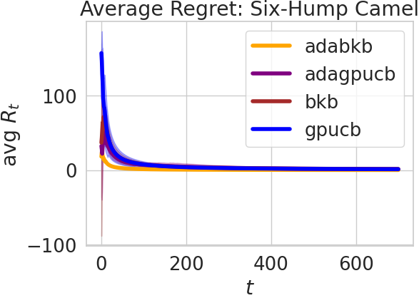
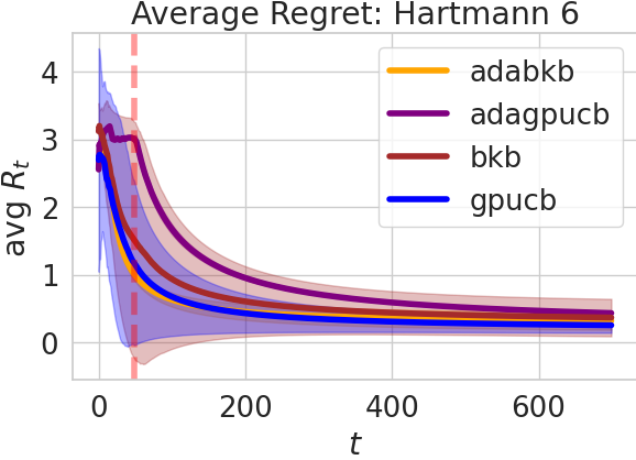
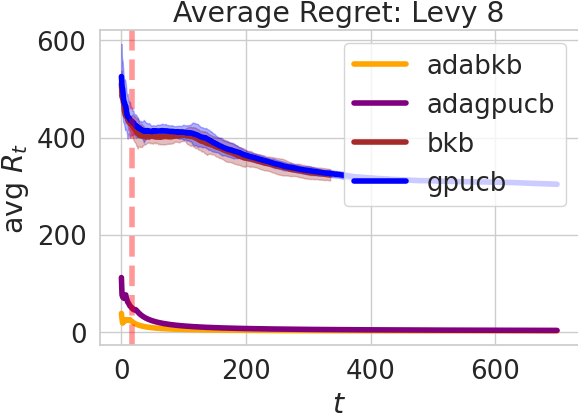
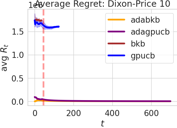
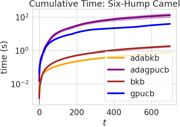
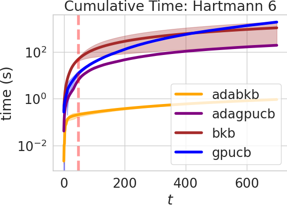
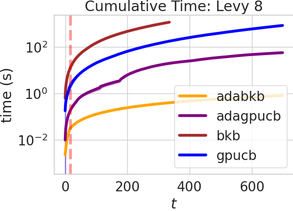
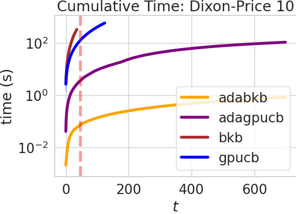
Figure 3: from left to right, average regret (first line) and cumulative time (second line) obtained by algorithms in optimizing, from top to bottom, Six-Hump Camel, Hartmann 6, Levy 8 and Dixon-Price 10 functions.

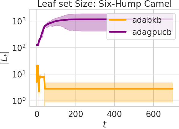
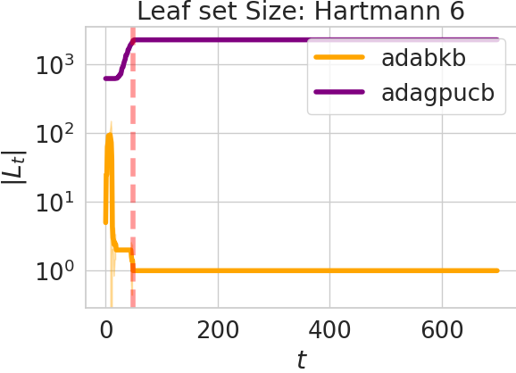
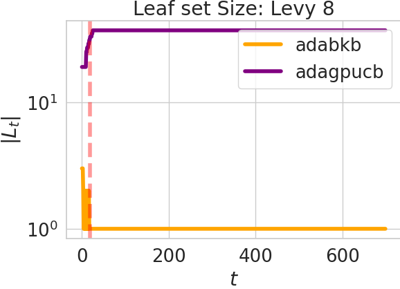
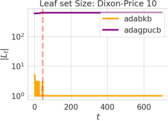
Figure 4: from left to right leaf set size of the algorithms in optimizing Six-Hump Camel, Hartmann 6, Levy 8 and Dixon-Price 10 functions.

For a budget $T$, in Figure 3 we show the average regret and the cumulative time per function evaluation. In Figure 4 we show the leaf set size per iteration for Ada-BKB and AdaGP-UCB. We added a time threshold of 600 seconds. The red vertical line in Figure 3 and 4, if present, indicates the (mean) iteration in which the early stopping condition is satisfied. We do not interrupt the execution just to show the behaviour of the algorithm (as you can notice in leaf set size plots, after the red line leaf set of Ada-BKB has cardinality $1$). From second column of Figure 3, we immediately note that AdaGP-UCB and Ada-BKB scale better with the search space dimension, but for low dimensional spaces (as Six-Hump Camel) AdaGP-UCB is more time consuming than GP-UCB. This is because for small dimensions we used small discretizations (15 points per dimension, see Appendix C) and hence the computations to build the matrices are cheap, while for the adaptive discretization we have to perform the expansion procedure. This is not necessarily always true for Ada-BKB thanks to the pruning procedure that let us balance the cost of expansion with the cost of evaluating the index. More experiments in Appendix C.4.

Hyper-parameter tuning.

We performed experiments to tune the hyper-parameters of a recently proposed large scale kernel method (Rudi et al.,, 2017). We compared Ada-BKB with AdaGP-UCB and BKB in minimizing the target function $f$ which takes as inputs a set of hyper-parameters to compute a hold-out cross-validation estimate of the error using 40% of the data. The method in (Rudi et al.,, 2017) is based on a Nyström approximation of kernel ridge regression. In our experiments, we used a Gaussian kernel $k$ and tuned a lengthscale parameters $\sigma_{1},\cdots,\sigma_{p}$ in each of the $p$ input dimensions. Indeed, we fixed the ridge parameters and the centers of the Nyström approximation (see Appendix C.2 for details). We considered also BKB on a random discretization of size equal to the number of points evaluated by Ada-BKB, called Random-BKB in the following. Again, for each experiment, we report mean and $95\%$ confidence interval using 5 repetitions. We added a time-threshold of 20 minutes.

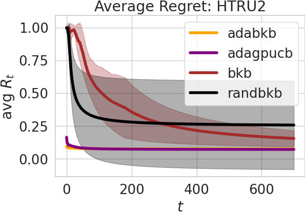
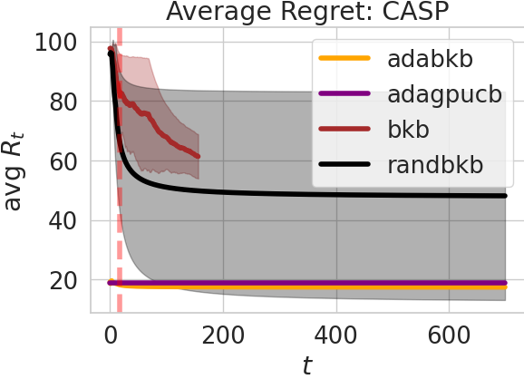
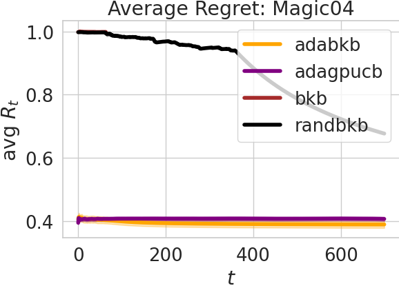
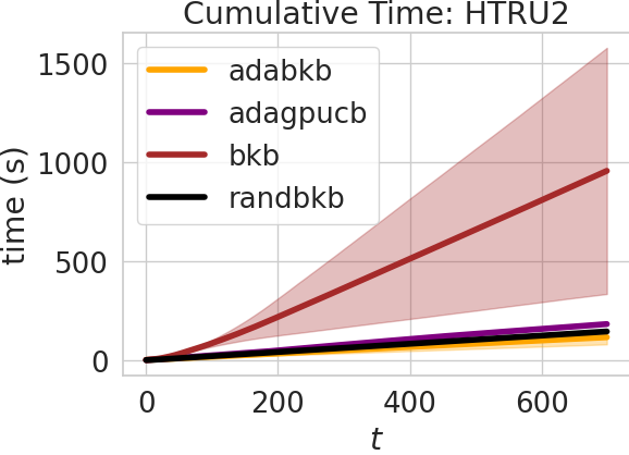
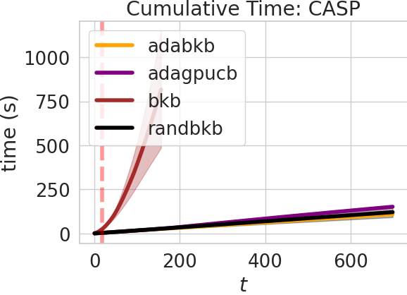
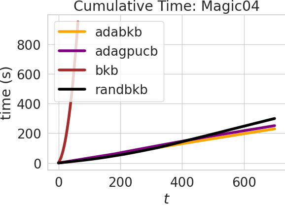
Figure 5: Average regret and cumulative time in optimizing the target function on HTRU2, CASP and Magic04 dataset.

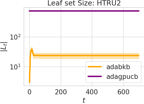
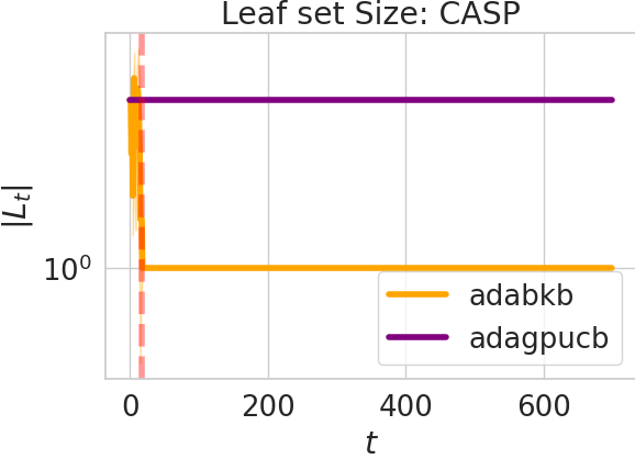
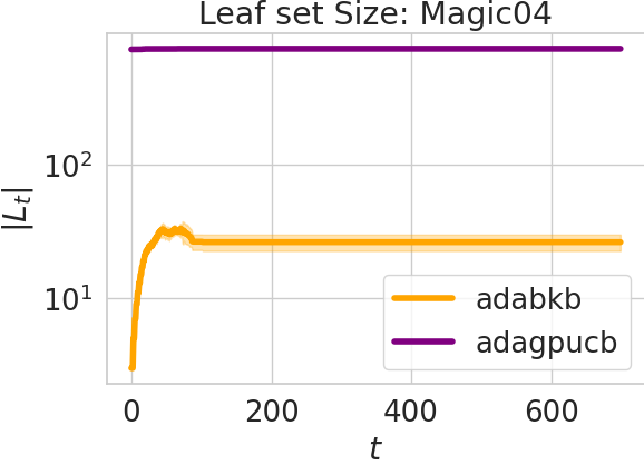
Figure 6: Leaf set size in optimizing the target function on HTRU2, CASP and Magic04 dataset.

In Figure 5, we note that Ada-BKB obtains smaller or similar regret to other algorithms. In terms of time, Ada-BKB is typically the fastest method. In some cases, we note that Random BKB can obtain similar time performance than Ada-BKB, but typically the regret is larger, see e.g. the first line of Figure 5. Finally, we report the test error obtained fitting the model with the hyper-parameter configuration found by Ada-BKB and the time nedeed to perform every function evaluation until the budget or the time threshold is reached.

Table 1: Mean $\pm$ standard deviation of test error (MSE) using the configuration found by the algorithms with $5$ repetition

ALGORITHM	HTRU2	CASP	MAGIC04
BKB	$0.067\pm 0.004$	$33.67\pm 17.79$	$0.99\pm 0.0005$
Random BKB	$0.24\pm 0.34$	$47.79\pm 35.81$	$0.412\pm 0.01$
Ada-BKB	0.068 $\pm$ 0.005	17.07 $\pm$ 0.09	0.383 $\pm$ 0.014
AdaGPUCB	$0.071\pm 0.003$	$18.65\pm 0.34$	$0.389\pm 0.010$

Table 2: Mean $\pm$ standard deviation of time (seconds) used for perform every function evaluation or before interruption with $5$ repetition

ALGORITHM	HTRU2	CASP	MAGIC04
BKB	$956.26\pm 622$	$818.21\pm 332$	$950.98\pm 1.30$
Random BKB	$144.47\pm 5.09$	$120.82\pm 28.85$	$299.63\pm 5.05$
Ada-BKB	115.21 $\pm$ 35.65	109.12 $\pm$ 1.09	230.06 $\pm$ 3.61
AdaGPUCB	$181.91\pm 1.81$	$151.57\pm 0.59$	$251.48\pm 0.65$

6 CONCLUSION

In this paper, we presented a scalable approach to Gaussian Process optimization on continuous domains, combining ideas from BKB and optimistic optimization. The proposed approach is analyzed theoretically in terms of regret guarantees, showing that improved efficiency can be achieved with no loss of accuracy. Empirically we report very good performances on both simulated data and a hyper-parameter tuning task. Our work opens a number of possible research directions. For example, efficiency could be further improved using experimentation batching, see (Calandriello et al.,, 2020). Another interesting question could be to extend the ideas in the paper to other way to define upper function estimates for example based on expected improvements (Qin et al.,, 2017).

Acknowledgments

This material is based upon work supported by the Center for Brains, Minds and Machines (CBMM), funded by NSF STC award CCF-1231216, and the Italian Institute of Technology. We gratefully acknowledge the support of NVIDIA Corporation for the donation of the Titan Xp GPUs and the Tesla k40 GPU used for this research. L. R. acknowledges the financial support of the European Research Council (grant SLING 819789), the AFOSR projects FA8655-20-1-7028, FA9550-18-1-7009, FA9550-17-1-0390 and BAA-AFRL-AFOSR-2016-0007 (European Office of Aerospace Research and Development), and the EU H2020-MSCA-RISE project NoMADS - DLV-777826. S. V. acknowledges the support of GNAMPA 2020: “Processi evolutivi con memoria descrivibili tramite equazioni integro-differenziali”

Appendix A AUXILIARY RESULTS

In the following, we state the propositions and lemmas required to prove Theorem 1.

Proposition 1.

(Calandriello et al.,, 2019, App. D, Theorem 9) Let $\epsilon\in(0,1)$, $\delta\in(0,1)$, $\lambda>0$, $F=\left\lVert{f}\right\rVert_{\mathcal{H}}$ and let $\bar{\alpha}=\frac{1+\epsilon}{1-\epsilon}$. Then, with probability at least $1-\delta$ and for all $t>0$:

$$\widetilde{\mu}_{t}(x)-{\beta}_{t}\widetilde{\sigma}_{t}(x)\leq f(x)\leq\widetilde{\mu}_{t}(x)+{\beta}_{t}\widetilde{\sigma}_{t}(x)$$

with

$$\beta_{t}=2\lambda^{2}\sqrt{\bar{\alpha}\log(\kappa^{2}t)\Big{(}\sum\limits_{s=1}^{t}\widetilde{\sigma}_{t}^{2}(x_{s})\Big{)}+\log(1/\delta)}+\Big{(}1+\frac{1}{\sqrt{1-\epsilon}}\Big{)}\sqrt{\lambda}F$$ (13)

We show that the index function $I_{t}(\cdot)$ (eq. (9)) is an upper bound on the maximum value of the function $f$ in a cell:

Proposition 2 (Upper bound on maximum of the function $f$).

Supposing Assumption 1 holds and assuming $f\in\mathcal{H}_{k}$, let $f(x^{*}_{h,i})$ be the maximum of $f$ in cell $X_{h,i}$ and let $x_{h,i}$ be a point in the same cell. For an arbitrary number of children per cell $N\geq 1$, setting $\beta_{t}$ as defined in Proposition 1 and with $V_{h}$ defined in equation (8), with probability at least $1-\delta$, for all $h\geq 0$, $1\leq i\leq N^{h}$ and for all $t>0$, we have:

$$f(x^{*}_{h,i})\leq I_{t}(x_{h,i})$$

with $I_{t}(\cdot)$ index function defined in (9)

Proof.

Let $p$ be the parent function of $(X_{h})_{h\in\mathbb{N}}$. For all $t>0$, the index function $I_{t}$ is defined as follow:

$$I_{t}(x_{h,i})=\min\{\tilde{\mu}_{t}(x_{h,i})+\beta_{t}\tilde{\sigma}_{t}(x_{h,i}),\tilde{\mu}_{t}(x_{p(h,i)})+\beta_{t}\tilde{\sigma}_{t}(x_{p(h,i)})+V_{h-1}\}+V_{h}$$

From the definition of $V_{h}$ (see equation (8)), for all $h\geq 0$ and $1\leq i\leq N^{h}$:

$$|f(x)-f(x^{\prime})|\leq\left\lVert{f}\right\rVert_{k}d_{k}(x,x^{\prime})\leq V_{h}\qquad\forall x,x^{\prime}\in X_{h,i}$$

where $d_{k}$ is defined in Assumption 1. Let $x^{*}_{h,i}$ be the maximizer of $f$ in cell $X_{h,i}$ and let $x_{h,i}$ be any point in $X_{h,i}$. It follows that $\forall h\geq 0$ and $1\leq i\leq N^{h}$:

$$f(x^{*}_{h,i})\leq f(x_{h,i})+V_{h}$$

Using Proposition 1 to upper bound $f(x^{*}_{h,i})$, it follows

$$f(x^{*}_{h,i})\leq\tilde{\mu}_{t}(x_{h,i})+\beta_{t}\tilde{\sigma}_{t}(x_{h,i})+V_{h}$$

for all $t>0$ (with probability at least $1-\delta$). For the same reason and by construction of the partition tree (Definition 1), we have:

$$f(x^{*}_{h,i})\leq\tilde{\mu}_{t}(x_{p(h,i)})+\beta_{t}\tilde{\sigma}_{t}(x_{p(h,i)})+V_{h-1}$$

where $V_{h-1}$ is an upper bound of the function variation at level $h-1$. Since $V_{h}\geq 0$,

$$f(x^{*}_{h,i})\leq\tilde{\mu}_{t}(x_{p(h,i)})+\beta_{t}\tilde{\sigma}_{t}(x_{p(h,i)})+V_{h-1}+V_{h}$$

∎

Remark 2.

Note that for the root cell $(0,1)$ the parent function is not defined. In this case, the index function is defined as:

$$I_{t}(x_{0,1})=\widetilde{\mu}_{t}(x_{0,1})+\beta_{t}\widetilde{\sigma}_{t}(x_{0,1})+V_{0}$$

Let $x^{*}$ be a global maximizer of the function $f$ and suppose $x^{*}\in X_{h,i^{*}}$. Let $x_{h,i^{*}}$ be the centroid of $X_{h,i^{*}}$. Then, Proposition 2 implies that with probability at least $1-\delta$,

$$f(x^{*})\leq I_{t}(x_{h,i^{*}})$$

Now, we procede providing an upper-bound $U_{V}$ of the ratio $\frac{V_{h}}{V_{h+1}}$ described by the following Proposition.

Proposition 3.

Suppose Assumption 2 holds and set $h_{0}=\frac{\log(\delta_{k}/v_{1})}{\log(\rho)}$. For all $h\geq 0$,

$$\frac{V_{h}}{V_{h+1}}\leq\max\Big{\{}\max\limits_{0\leq h\leq h_{0}-1}\frac{V_{h}}{V_{h+1}},\frac{C^{\prime}_{k}}{C_{k}}\rho^{-\alpha}\Big{\}}=:U_{V}$$ (14)

Proof.

Using the definition of $V_{h}$ (Equation (8)), we can write the ratio as:

$$\frac{V_{h}}{V_{h+1}}=\frac{Fg(v_{1}\rho^{h})}{Fg(v_{1}\rho^{h+1})}=\frac{g(v_{1}\rho^{h})}{g(v_{1}\rho^{h+1})}$$

Now, we have that $\exists\delta_{k}>0$ such that:

$$C_{k}v_{1}^{\alpha}\rho^{h\alpha}\leq g(v_{1}\rho^{h})\leq C^{\prime}_{k}v_{1}^{\alpha}\rho^{h\alpha}\qquad\forall v_{1}\rho^{h}\leq\delta_{k}$$

then for all $v_{1}\rho^{h}$ lower than $\delta_{k}$, we can write:

$$\frac{V_{h}}{V_{h+1}} =\frac{g(v_{1}\rho^{h})}{g(v_{1}\rho^{h+1})}$$ (15)

$$\leq\frac{C^{\prime}_{k}v_{1}^{\alpha}\rho^{h\alpha}}{C_{k}v_{1}^{\alpha}\rho^{h\alpha+\alpha}}$$ (16)

$$=\frac{C^{\prime}_{k}}{C_{k}}\frac{1}{\rho^{\alpha}}=\frac{C^{\prime}_{k}}{C_{k}}\rho^{-\alpha}$$ (17)

Now, to conclude the proof, it is enough to observe that in Assumption 2

$$(\forall h\geq h_{0})\qquad v_{1}\rho^{h}\leq\delta_{k}$$

For $h<h_{0}$, we can upper bound the ratio $\frac{V_{h}}{V_{h+1}}$ just with the maximum of the ratios for all $h\in[0,h_{0}-1]$. So the statement follows.∎

Proposition 3 states that $\forall h\geq 0$ we have $V_{h}\leq U_{V}V_{h+1}$ and this fact is exploited in the following lemma which give us information about the points selected by the algorithm.

Lemma 2.

Suppose that Assumptions 1,2,3 hold. Set $\beta_{t}$ as in eq. (13), define $V_{h}$ as in (8), and let $f(x^{*})$ be the global maximum of $f$. If at time $t$, $x_{h_{t},i_{t}}\in L_{\tau}$ is evaluated then with probability at least $1-\delta$:

$$f(x^{*})-f(x_{h_{t},i_{t}})\leq(4U_{V}+1)V_{h_{t}}$$

Moreover, if $h<h_{\text{max}}$ then

$$f(x^{*})-f(x_{h_{t},i_{t}})\leq 3\beta_{t}\tilde{\sigma}_{t}(x_{h_{t},i_{t}})$$

Proof.

According to the Proposition 1, setting $\beta_{t}$ as in eq. (13), we have that

$$\tilde{\mu}_{t}(x)-\beta_{t}\tilde{\sigma}_{t}(x)\leq f(x)\leq\tilde{\mu}_{t}(x)+\beta_{t}\tilde{\sigma}_{t}(x)$$

with probability of $1-\delta$. From equation (8)), we have for all $h\geq 0$ and $1\leq i\leq N^{h}$:

$$\sup\limits_{x_{1},x_{2}\in X_{h,i}}|f(x_{1})-f(x_{2})|\leq V_{h}$$

Suppose that at time $t$ $x^{*}$ is contained in the cell $X_{h^{*}_{t},i^{*}_{t}}$ represented by $x_{h^{*}_{t},i^{*}_{t}}\in L_{\tau}$ and that the algorithm selects and evaluate the point $x_{h_{t},i_{t}}$. From Proposition 2, with probability at least $1-\delta$, we have that

$$f(x^{*})\leq I_{t}(x_{h^{*}_{t},i^{*}_{t}}).$$ (18)

Since the algorithm selected $x_{h_{t},i_{t}}$, according to the selection rule (row 5 of Algorithm 1) it follows that

$$I_{t}(x_{h^{*}_{t},i^{*}_{t}})\leq I_{t}(x_{h_{t},i_{t}}).$$ (19)

We recall that $I_{t}$ is defined as:

$$I_{t}(x_{h_{t},i_{t}})=\min\{\tilde{\mu}_{t}(x_{h_{t},i_{t}})+\beta_{t}\tilde{\sigma}_{t}(x_{h_{t},i_{t}}),\tilde{\mu}_{t}(x_{p(h_{t},i_{t})})+\beta_{t}\tilde{\sigma}_{t}(x_{p(h_{t},i_{t})})+V_{h_{t}-1}\}+V_{h_{t}}$$

therefore

$$f(x^{*})\leq I_{t}(x_{h^{*}_{t},i^{*}_{t}})\leq I_{t}(x_{h_{t},i_{t}})\leq\tilde{\mu}_{t}(x_{p(h_{t},i_{t})})+\beta_{t}\tilde{\sigma}_{t}(x_{p(h_{t},i_{t})})+V_{h_{t}-1}+V_{h_{t}}.$$ (20)

In the rest of the proof we upper bound the right hand side. Proposition 1, yields (with probability at least $1-\delta$):

$$f(x_{p(h_{t},i_{t})})\geq\tilde{\mu}_{t}(x_{p(h_{t},i_{t})})-\beta_{t}\tilde{\sigma}_{t}(x_{p(h_{t},i_{t})}),$$

and therefore

$$\tilde{\mu}_{t}(x_{p(h_{t},i_{t})})+\beta_{t}\tilde{\sigma}_{t}(x_{p(h_{t},i_{t})})+V_{h_{t}-1}+V_{h_{t}}\leq f(x_{p(h_{t},i_{t})})+2\beta_{t}\tilde{\sigma}_{t}(x_{p(h_{t},i_{t})})+V_{h_{t}-1}+V_{h_{t}}$$ (21)

Since the algorithm evaluated $x_{h_{t},i_{t}}$, then $\tilde{\beta}\tilde{\sigma}_{t}(x_{p(h_{t},i_{t})})\leq V_{h_{t}-1}$ therefore

$$f(x_{p(h_{t},i_{t})})+2\beta_{t}\tilde{\sigma}_{t}(x_{p(h_{t},i_{t})})+V_{h_{t}-1}+V_{h_{t}}\leq(f(x_{p(h_{t},i_{t})})+V_{h_{t}-1})+2V_{h_{t}-1}+V_{h_{t}}$$ (22)

By construction of the partition tree, $x_{h_{t},i_{t}}$ lies in the cell associated to $x_{p(h_{t},i_{t})}$, and so $f(x_{p(h_{t},i_{t})})\leq f(x_{h_{t},i_{t}})+V_{h_{t}}$. Hence,

$$(f(x_{p(h_{t},i_{t})})+V_{h_{t}-1})+2V_{h_{t}-1}+V_{h_{t}}\leq f(x_{h_{t},i_{t}})+4V_{h_{t}-1}+V_{h_{t}}$$ (23)

and, using Proposition 3:

$$f(x_{h_{t},i_{t}})+4V_{h_{t}-1}+V_{h_{t}}\leq f(x_{h_{t},i_{t}})+(4U_{V}+1)V_{h_{t}}.$$ (24)

The latter combined with (20), implies that

$$f(x^{*})\leq f(x_{h_{t},i_{t}})+(4U_{V}+1)V_{h_{t}}.$$ (25)

To prove the second bound of the statement, note that

$$I_{t}(x_{h^{*}_{t},i^{*}_{t}})\leq I_{t}(x_{h_{t},i_{t}})\leq\tilde{\mu}_{t}(x_{h_{t},i_{t}})+\beta_{t}\tilde{\sigma}_{t}(x_{h_{t},i_{t}})+V_{h_{t}}$$ (26)

Proposition 1 yields that, with probability at least $1-\delta$

$$f(x_{h_{t},i_{t}})\geq\tilde{\mu}_{t}(x_{h_{t},i_{t}})-\beta_{t}\tilde{\sigma}_{t}(x_{h_{t},i_{t}})$$

then it follows:

$$\tilde{\mu}_{t}(x_{h_{t},i_{t}})+\beta_{t}\tilde{\sigma}_{t}(x_{h_{t},i_{t}})+V_{h_{t}}\leq f(x_{h_{t},i_{t}})+2\beta_{t}\tilde{\sigma}_{t}(x_{h_{t},i_{t}})+V_{h_{t}}$$ (27)

Next, if $h<h_{\text{max}}$, since $x_{h_{t},i_{t}}$ is evaluated, then $\beta_{t}\tilde{\sigma}_{t}(x_{h_{t},i_{t}})>V_{h_{t}}$, and

$$f(x^{*})\leq\tilde{\mu}_{t}(x_{h_{t},i_{t}})+2\beta_{t}\tilde{\sigma}_{t}(x_{h_{t},i_{t}})+V_{h_{t}}\leq f(x_{h_{t},i_{t}})+3\beta_{t}\tilde{\sigma}_{t}(x_{h_{t},i_{t}})$$ (28)

In conclusion, we derive that if $h<h_{\text{max}}$

$$f(x^{*})-f(x_{h_{t},i_{t}})\leq 3\beta_{t}\tilde{\sigma}_{t}(x_{h_{t},i_{t}}).$$

∎

Proposition 4.

(Calandriello et al.,, 2019, Theorem 2) For any desired $0<\epsilon<1$, $0<\delta<1$, $\lambda>0$, let $\bar{\alpha}=\frac{1+\epsilon}{1-\epsilon}$. For $\beta_{t}$ defined as :

$$\beta_{t}=2\lambda^{2}\sqrt{\bar{\alpha}\log(\kappa^{2}t)\Big{(}\sum\limits_{s=1}^{t}\widetilde{\sigma}_{t}^{2}(x_{s})\Big{)}+\log(1/\delta)}+\Big{(}1+\frac{1}{\sqrt{1-\epsilon}}\Big{)}\sqrt{\lambda}F$$

and $\tilde{\sigma}_{t}$ defined as in equation (5) we have that:

$$3\tilde{\beta}_{T}\sum\limits_{t=1}^{T}\tilde{\sigma}_{t}(x_{t})\leq\mathcal{O}(\sqrt{T}d_{\text{eff}}(\lambda,\tilde{X}_{T})\log T)$$

where $\tilde{X}_{T}$ is the set containing every centroid evaluated until timestep $T$.

Proposition 5 (Standard deviation upper bound).

Consider the evaluation model $y_{t}=f(x_{t})+\eta_{t}$ with $\eta_{t}\sim\mathcal{N}(0,\sigma^{2})$, and let be $n_{t}:X\rightarrow\mathbb{N}$ a function which given a centroid $x_{h,i}$ returns the number of times that it has been evaluated until time step $t$. For a desired $\epsilon\in(0,1)$, let $\bar{\alpha}=\frac{1+\epsilon}{1-\epsilon}$. Then, if a centroid $x_{h,i}$ is evaluated $n_{t}(x_{h,i})$ times we have

$$\widetilde{\sigma}_{t}(x_{h,i})\leq\sqrt{\bar{\alpha}}\frac{\sigma}{\sqrt{n_{t}(x_{h,i})}}$$

Proof.

(Shekhar and Javidi,, 2018, Part 1 of Proposition 3) yields

$$\sigma_{t}(x_{h,i})\leq\frac{\sigma}{\sqrt{n_{t}(x_{h,i})}}$$

where $\sigma_{t}$ is defined as in eq. (3). (Calandriello et al.,, 2019, Theorem 1) implies that for a desired $\epsilon\in(0,1)$, setting $\bar{\alpha}=\frac{1+\epsilon}{1-\epsilon}$, $\tilde{\sigma}^{2}(x)$ defined in eq. (5) satisfies the following inequality:

$$\tilde{\sigma}_{t}^{2}(x)\leq\bar{\alpha}\sigma_{t}^{2}(x)$$

Which gives

$$\tilde{\sigma}_{t}(x)\leq\sqrt{\bar{\alpha}}\sigma_{t}(x)\leq\sqrt{\bar{\alpha}}\frac{\sigma}{\sqrt{n_{t}(x)}}$$

∎

Appendix B PROOFS OF MAIN RESULTS

In this appendix, we provide the proofs of Lemma 1 and Theorems 12.

B.1 Proof of Lemma 1

For all $x,x^{\prime}\in X_{h,i}$,

$$|f(x)-f(x^{\prime})|=|\left\langle{f},{k(x,\cdot)-k(x^{\prime},\cdot)}\right\rangle|\leq\left\lVert{f}\right\rVert d_{k}(x,x^{\prime})\leq\left\lVert{f}\right\rVert g(d(x,x^{\prime}))\leq\left\lVert{f}\right\rVert g(v_{1}\rho^{h})$$

B.2 Proof of Theorem 1

To prove the bound on the cumulative regret we need to introduce some objects. First, denoting with $x_{h_{t},i_{t}}$ the centroid of $X_{h_{t},i_{t}}$ evaluated at function evaluation $t$, let’s define $Q_{T}$ as the set containing every point evaluated at each function evaluation:

$$Q_{T}=\{x_{h_{t},i_{t}}|1\leq t\leq T\}$$

Now, we split $Q_{T}$ in two sets $Q_{1},Q_{2}$ defined as follow:

$$Q_{1} =\{x_{h,i}\in Q_{T}|h<h_{\text{max}}\}$$ (29)

$$Q_{2} =Q_{T}\setminus Q_{1}$$

So, we consider separately the terms which contribute to the cumulative regret:

$$R_{T}=\sum\limits_{x\in Q_{T}}f(x^{*})-f(x)=\sum\limits_{x\in Q_{1}}f(x^{*})-f(x)+\sum\limits_{x\in Q_{2}}f(x^{*})-f(x)=R_{1}+R_{2},$$

where

$$R_{1}=\sum\limits_{x\in Q_{1}}f(x^{*})-f(x)\qquad\text{and}\qquad R_{2}=\sum\limits_{x\in Q_{2}}f(x^{*})-f(x).$$

Let’s start by bounding $R_{2}$. Using Lemma 2, we can upper-bound $R_{2}$ as:

$$R_{2}=\sum\limits_{x\in Q_{2}}f(x^{*})-f(x)\leq(4U_{V}+1)V_{h_{\text{max}}}|Q_{2}|$$

The size of $Q_{2}$ can be trivially upper-bounded with the budget $T$:

$$(4U_{V}+1)V_{h_{\text{max}}}|Q_{2}|\leq(4U_{V}+1)V_{h_{\text{max}}}T$$

Noting that $h_{\text{max}}\geq h_{0}$, Assumption 2 implies

$$(4U_{V}+1)V_{h_{\text{max}}}T\leq(4U_{V}+1)C^{\prime}_{k}v_{1}^{\alpha}\rho^{h_{\text{max}}\alpha}T\leq\mathcal{O}(\rho^{h_{\text{max}}\alpha}T)$$

Moreover, since $h_{\text{max}}\geq\frac{1/2\log T}{\alpha\log 1/\rho}$,

$$\rho^{h_{\text{max}}\alpha}T\leq\sqrt{T\log T}$$

To upper-bound $R_{1}$, since $|Q_{1}|\leq T$, Lemma 2 yields:

$$R_{1}=\sum\limits_{x\in Q_{1}}f(x^{*})-f(x)\leq 3\sum\limits_{x_{h_{t},i_{t}}\in Q_{1}}\tilde{\beta}_{t}\tilde{\sigma}_{t}(x)$$

Again, since $|Q_{1}|\leq T$, we get

$$3\sum\limits_{x_{h_{t},i_{t}}\in Q_{1}}\tilde{\beta}_{t}\tilde{\sigma}_{t}(x_{h_{t},i_{t}})\leq 3\sum\limits_{t=1}^{T}\tilde{\beta}_{t}\tilde{\sigma}_{t}(x_{h_{t},i_{t}})\leq 3\tilde{\beta}_{T}\sum\limits_{t=1}^{T}\tilde{\sigma}_{t}(x_{h_{t},i_{t}})$$

Proposition 4 implies

$$3\tilde{\beta}_{T}\sum\limits_{t=1}^{T}\tilde{\sigma}_{t}(x_{h_{t},i_{t}})\leq\mathcal{O}(\sqrt{T}d_{\text{eff}}(T)\log T)$$

Summing $R_{1}$ and $R_{2}$:

$$R_{T} =R_{1}+R_{2}$$

$$\leq\mathcal{O}(\sqrt{T}d_{\text{eff}}(T)\log T+\sqrt{T\log T})$$

$$\leq\mathcal{O}(\sqrt{T}d_{\text{eff}}(T)\log T)$$

Now assume that the evaluation model is

$$y_{t}=f(x_{t})+\eta_{t}\qquad\text{with }\eta_{t}\sim\mathcal{N}(0,\sigma^{2})$$

In this scenario, We follow a similar proof strategy of (Salgia et al.,, 2020, Proof of Lemma 1). Let $Q_{1}$ be the set of observed centroids at depth $h<h_{\text{max}}$ (eq. (29)) and let $n_{i}$ be the number of times that the $i$-th centroid (in the set $Q_{1}$) has been evaluated. Let $J$ be the set containing the indices of distinct points evaluated at least one time at depth $h<h_{\text{max}}$:

$$J=\{j:n_{i}>0\}.$$

It follows $|J|\leq\frac{N^{h_{\text{max}}}-1}{N-1}$, which corresponds to the case in which Ada-BKB evaluates every point in the partition tree with maximum depth $h_{\text{max}}-1$. Considering $x_{i}$ as the $i$-th centroid in $Q_{1}$, let’s denote with $t_{j}$ the time in which $x_{i}$ has been selected and evaluated for the $j$-th time at timestep $t$ i.e. for all $2\leq j\leq n_{i}$, at timestep $t_{j}$, the centroid $x_{i}$ has been evaluated $j-1$ times. By Proposition 5, we have that

$$\tilde{\sigma}_{t_{j}-1}(x_{t_{j}})\leq\sqrt{\alpha}\frac{\sigma^{2}}{\sqrt{j-1}}.$$

The contribution of every point $x_{j}$ with $j\in J$ to the sum of approximate variances is upper bounded by

$$1+\sqrt{\alpha}\sigma^{2}_{n}\sum\limits_{i=1}^{n_{j}-1}\frac{1}{\sqrt{i}}$$ (30)

Lemma 2 implies

$$R_{1}=\sum\limits_{x\in Q_{1}}f(x^{*})-f(x)\leq 3\tilde{\beta}_{T}\sum\limits_{t=1}^{T}\tilde{\sigma}_{t-1}(x_{(h_{t},i_{t})})$$

We derive from (30) that

$$R_{1} \leq 3\tilde{\beta}_{T}\sum\limits_{j\in J}\Bigg{(}(1+\sqrt{\bar{\alpha}}\sigma^{2})\sum\limits_{k=1}^{n_{j}-1}\frac{1}{\sqrt{k}}\Bigg{)}$$

$$\leq 3\tilde{\beta}_{T}\sum\limits_{j\in J}\Bigg{(}(1+2\sqrt{\bar{\alpha}}\sigma^{2})\sqrt{n_{j}-1}\Big{)}$$

$$\leq 3\tilde{\beta}_{T}(1+2\sqrt{\bar{\alpha}}\sigma^{2})\sum\limits_{j\in J}\sqrt{n_{j}}$$

By Jensen’s inequality,

$$R_{1} \leq 3\tilde{\beta}_{T}(1+2\sqrt{\bar{\alpha}}\sigma^{2})|J|\sqrt{\frac{1}{|J|}\sum\limits_{j\in J}n_{j}}$$

$$\leq 3\tilde{\beta}_{T}(1+2\sqrt{\bar{\alpha}}\sigma^{2})\sqrt{|J|T}$$

$$\leq 3\tilde{\beta}_{T}(1+2\sqrt{\bar{\alpha}}\sigma^{2})\sqrt{\frac{N^{h_{\text{max}}}-1}{N-1}T}$$

(Calandriello et al.,, 2019, Appendix D.2) implies that

$$\tilde{\beta}_{T}\leq 2\lambda\sqrt{d_{\text{eff}}\log(k^{2}T)+\log(1/\delta)}+(1+\frac{1}{\sqrt{1-\epsilon}})\sqrt{\lambda}F$$

Therefore,

$$R_{1}\leq\mathcal{O}\Bigg{(}\sqrt{Td_{\text{eff}}\log(k^{2}T)\frac{N^{h_{\text{max}}}-1}{N-1}}+\sqrt{T\frac{N^{h_{\text{max}}}-1}{N-1}}\Bigg{)}$$

If we take $N>1$ s.t. $\sqrt{\frac{N^{h_{\text{max}}}-1}{N-1}}<T$, we derive from (B.2) that

$$\mathcal{O}\Bigg{(}\sqrt{Td_{\text{eff}}\log(k^{2}T)\frac{N^{h_{\text{max}}}-1}{N-1}}\Bigg{)}$$

Notice that $\sqrt{\frac{N^{h_{\text{max}}}-1}{N-1}}$ doesn’t grow with $p$ (search space dimension) as $d_{\text{eff}}$.

B.3 Proof of Theorem 2

Let $j$ be the number of observations at a certain time step. We analyze the sources of cost of Algorithm 1 to get the computational cost.

Model update.

According to the algorithm, every time we evaluate the function (i.e. we observe $y=f(x)+\eta$), we update our model. With BKB (Calandriello et al.,, 2019), we know that an update consists in recomputing $\tilde{\mu}$, $\tilde{\sigma}$ and in ”resparsificating” the approximation. As indicated in (Calandriello et al.,, 2019), the computational cost of performing these operations is $\mathcal{O}(Td_{\text{eff}}^{2}(T))$.

Index computation.

The computation of the index is the most expensive operation, see (Shekhar and Javidi,, 2018). In order to get a similar analysis to AdaGP-UCB, we consider the total cost of computing $I_{t}$. Since the cost of evaluating $\tilde{\mu}_{t},\tilde{\sigma}_{t}$ for a point is $\mathcal{O}(d_{\text{eff}}^{2}(T))$, let’s analyze two different scenarios:

1. Refinement steps: if we have expanded a node, we don’t perform an update of the model, so we can compute the index only for the new nodes (i.e. we just compute the approximated mean and variance for new nodes). Each refinement operation adds $N$ new points to the leaf set and remove the expanded node, thus, the overall computational cost is:

   $$\mathcal{O}(Td_{\text{eff}}^{2}(T)(N-1)h_{\text{max}})$$

2. Evaluation steps: after an evaluation, we update our model and, we have to recompute the index for the entire leaf set. In the worst case, the leaf set $L_{\tau}$ at time $t$ contains every representative point of the nodes of the partition tree at depth $h_{\text{max}}$ and since the sub-tree of partition tree at depth $h_{\text{max}}$ (and at any $h\geq 0$) is a perfect $N$-ary tree,

   $$|L_{\tau}|\leq N^{h_{\text{max}}}.$$

   So, the overall computational cost is:

   $$\mathcal{O}(Td_{\text{eff}}^{2}(T)N^{h_{\text{max}}}).$$

Candidate selection.

The selection procedure consists in chosing the $x\in L_{\tau}$ which maximize $I_{t}$, i.e.:

$$\operatornamewithlimits{arg\,max}\limits_{x\in L_{\tau}}I_{t}(x)$$

Ignoring the cost of computing the index (since we analyzed it in the previous point), we have to consider the cost of computing the argmax in case we did refinement steps or evaluation steps:

1. Refinement steps: after refinement steps, the model is not changed so we can take the argmax of new nodes (since the previous maximizer was the expanded node) and this costs $\mathcal{O}((N-1)h_{\text{max}}T)$.

2. Evaluation steps: we have to perform an exhaustive search on the leaf set and, this will cost:

   $$\mathcal{O}(TN^{h_{\text{max}}})$$

Search space refinement.

When $X\subset\mathbb{R}^{p}$, the refinement of a cell $X_{h,i}$ is performed by dividing it equally in $N$ parts along its longest side (see also (Shekhar and Javidi,, 2018)). This operation involves specifying the centers and the $p$ side lengths of each of the $N$ new cells and is thus a $\mathcal{O}(pN)$ operation. So the overall cost of search space refinement is:

$$\mathcal{O}(Th_{\text{max}}Np)$$

So, the total cost for the algorithm is $\mathcal{O}(Td_{\text{eff}}^{2}(T)N^{h_{\text{max}}}+Th_{\text{max}}Np)$ and thus, fixed $p$:

$$\mathcal{O}(Td_{\text{eff}}^{2}(T)N^{h_{\text{max}}})$$

Appendix C EXPERIMENT DETAILS

In this appendix, we describe the optimizer settings used to perform experiments presented in Section 5, showing also other experiments performed. Every experiment is realized in Python 3.6.9 using sklearn(Pedregosa et al.,, 2011; Buitinck et al.,, 2013), pytorch(Paszke et al.,, 2017), gpytorch(Gardner et al.,, 2018) and numpy(Harris et al.,, 2020) libraries.
The implementation of BKB used can be found on GitHub at the following link https://github.com/luigicarratino/batch-bkb

C.1 Synthetic experiments details

Synthetic experiments consist in finding global minima in well-known function, in particular, we considered the following functions and search spaces:

Table 3: Function used and relative search space considered for Ada-BKB and AdaGP-UCB.

FUNCTION	SEARCH SPACE $X$
Branin	$[-5.0,10.0]\times[0.0,15.0]$
Beale	$[-4.5,4.5]^{2}$
Bohachevsky	$[-10.0,190.0]\times[-180.0,20.0]$
Rosenbrock 2	$[-5.0,10.0]^{2}$
Six-Hump Camel	$[-2.0,2.0]\times[-3.0,3.0]$
Ackley 2	$[-10.0,52.768]^{2}$
Trid 2	$[-4.0,4.0]^{2}$
Hartmann 3	$[0.0,1.0]^{3}$
Trid 4	$[-16.0,16.0]^{4}$
Shekel	$[0.0,10.0]^{4}$
Ackley 5	$[-10.0,52.768]^{5}$
Hartmann 6	$[0.0,1.0]^{6}$
Levy 6	$[-10.0,10.0]^{6}$
Levy 8	$[-10.0,10.0]^{8}$
Rastrigin 8	$[-1.12,5.12]^{8}$
Dixon-Price 10	$[-10.0,10.0]^{10}$
Ackley 30	$[-10.0,52.768]^{30}$

The parameter $\delta$ is set to $10^{-5}$ for every experiments.

Table 4: Parameters of the optimizer used for experiments presented in Section 5 and Appendix C.4.

FUNCTION	$\sigma$	$h_{\text{max}}$	$N$	$p$
Branin	$0.5$	$5$	$3$	$2$
Beale	$1.0$	$5$	$3$	$2$
Bohachevsky	$1.70$	$9$	$3$	$2$
Rosenbrock 2	$0.70$	$10$	$11$	$2$
Six-Hump Camel	$0.5$	$6$	$5$	$2$
Ackley 2	$3.5$	$7$	$3$	$2$
Trid 2	$1.5$	$7$	$5$	$2$
Hartmann 3	$0.5$	$7$	$3$	$3$
Trid 4	$10.75$	$7$	$13$	$4$
Shekel	$1.75$	$6$	$9$	$4$
Ackley 5	$5.0$	$6$	$3$	$5$
Hartmann 6	$0.35$	$5$	$5$	$6$
Levy 6	$5.0$	$7$	$5$	$6$
Levy 8	$2.5$	$7$	$3$	$8$
Rastrigin 8	$7.0$	$10$	$3$	$8$
Dixon-Price 10	$2.0$	$10$	$5$	$10$
Ackley 30	$20.50$	$300$	$3$	$30$

Detailed information about the test functions is available at the following website: https://www.sfu.ca/~ssurjano/optimization.html.
For every algorithm, we used a Gaussian kernel with lengthscale $\sigma$ specified in Table 4. The noise standard deviation (indicated with $\lambda$) is set to $0.01$ for every experiment. Values for other parameters (like the kernel lengthscale $\sigma$) specified in Table 4 are obtained using cross-validation (the value of $h_{\text{max}}$ is just the logarithm of the budget).
For GP-UCB and BKB, the discrete search space was built by taking $15$ points for every dimension and computing the Cartesian product. For ”mid dimensional” cases (5 and 6 dimensions), the number of points per dimension taken is $10$ and for higher dimensional spaces $5$ points per dimension are taken .
The parameter $F$ is set to be $1$.

C.2 Hyper-parameter tuning experiments details

For FALKON hyper-parameter tuning experiments, we used the following datasets

Table 5: Dataset used with number of features and search spaces considered

DATASET	$p$	SEARCH SPACE
HTRU2	$8$	$[0.0,1.0]^{8}$
CASP	$9$	$[0.0,1.0]^{9}$
Magic04	$10$	$[0.1,10.0]^{10}$

In following tables, for each dataset, we indicate the number of rows, size for the training and test part and we also indicate the value for $M$ and $\lambda$ (Falkon parameters) used:

Table 6: Falkon fixed parameter per dataset used and size of dataset and relative training and test parts

DATASET	ROWS	TRAINING	TEST	M	$\lambda$
HTRU2	$17897$	$15216$	$3804$	$1000$	$1e-5$
CASP	$45730$	$32010$	$13720$	$2000$	$1e-5$
Magic04	$19020$	$14317$	$3580$	$2000$	$1e-6$

Table 7: parameter for the optimizer used for parameter tuning experiments

DATASET	$\sigma$	$\lambda$	$h_{\text{max}}$	$N$	$\delta$
HTRU2	$10.0$	$1e-9$	$6$	$3$	$1e-5$
CASP	$5.0$	$1e-9$	$7$	$5$	$1e-5$
Magic04	$5.0$	$1e-9$	$6$	$3$	$1e-5$

Again, the parameter $F$ is set to be $1$. We used a Gaussian kernel $k$ with many lengthscale parameters $\sigma_{1},\cdots,\sigma_{p}$ with $p$ number of features of the dataset

$$k(x,x^{\prime})=e^{-\frac{1}{2}x\Sigma^{-1}x^{\prime}}\qquad\Sigma=\begin{bmatrix}\sigma^{2}_{1}&0&\cdots&0\\ 0&\sigma^{2}_{2}&\cdots&0\\ \vdots&\vdots&\ddots&\vdots\\ 0&0&\cdots&\sigma^{2}_{p}\end{bmatrix}$$

Target function $f$ used is the $70$-$30$ hold-out cross-validation which splits the training set in training and validation where:

1. training part is composed by the $70\%$ of the points of the training set and it is used to fit the model.

2. validation part is composed of the remaining $30\%$ of the points of the training set and it is used to test our model fitted with the training part.

Before splitting the training set, it is shuffled. The metric used to evaluate the model is the mean square error (MSE) which, given $y$ corresponding labels of the validation part and $\tilde{y}$ the label predicted by the model (on the validation part) is defined as follow:

$$MSE(y,\tilde{y})=\frac{1}{n}\sum\limits_{i=1}^{n}(y_{i}-\tilde{y}_{i})^{2}$$

Thus, we want to minimize the function $f$ which takes a parameter configuration, performs the hold-out cross-validation, and returns the MSE. Since, we don’t know which is the best parameter configuration and how large is the minimum MSE, to compute the average regret we assume that let $x^{*}$ be the optimal configuration, then $f(x^{*})=0$. We don’t expect that our algorithm finds this configuration (also because it could not exist) but this strategy allows us to see which algorithm get the highest performance. As for synthetic experiments, the parameters of the optimizer (Table 7) are set using the value suggested by the theory and using cross-validation (for the number of children per node $N$, kernel lengthscale $\sigma$, etc) when it wasn’t possible. Falkon library (Meanti et al.,, 2020) used can be found at following url: https://github.com/FalkonML/falkon (in particular, since dataset used are small enough, to speed-up computations we used InCore Falkon (Meanti et al.,, 2020)). Dataset used to perform experiments are split in training and test part (described in Table 6). Preprocessing mostly consisted of data standardization to zero mean and unit standard deviation and, when a dataset is used for binary classification, labels are set to be $-1$ and $1$ (for instance for Magic04 dataset where labels are ’g’ and ’h’). Dataset used can be downloaded at the following links:

1. HTRU2 (Lyon et al.,, 2016; Dua and Graff,, 2017): https://archive.ics.uci.edu/ml/datasets/HTRU2

2. CASP (Dua and Graff,, 2017): https://archive.ics.uci.edu/ml/datasets/Physicochemical+Properties+of+Protein+Tertiary+Structure

3. Magic04 (Dua and Graff,, 2017): https://archive.ics.uci.edu/ml/datasets/MAGIC+Gamma+Telescope

For each dataset, we estimated also the evaluation time of the target function on random parameter configuration to get an idea about how much this target function is expensive in time:

Table 8: mean $\pm$ standard deviation time of evaluating the target function $f$ with a random configuration with $50$ repetition

DATASET	FUNCTION EVALUATION
HTRU2	$0.1877\pm 0.4682s$
CASP	$0.2562\pm 0.4565s$
Magic04	$0.1971\pm 0.4565s$

C.3 Machines used for experiments

In the following tables, we describe the features of the machine used to perform the experiments presented in Section 5 and Appendix C.4.

Table 9: machine used to perform the experiments

FEATURE
OS	Ubuntu 18.04.1
CPU(s)	$2\times$ Intel(R) Xeon(R) Silver 4116 CPU
RAM	$256$GB
GPU(s)	$2\times$ NVIDIA Titan Xp (12 GB RAM)
CUDA version	$10.2$

Further details of GPUs used can be found in the following links: https://www.nvidia.com/en-us/titan/titan-xp/

C.4 Other experiments

We performed other experiments in minimizing well-known functions specified in Table 3. Again, for showing better the results, we just plot the first $700$ evaluations. The red vertical dashed line indicates when the early stopping condition is satisfied. We added a time threshold of 600 seconds.

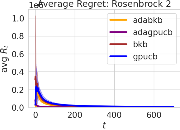
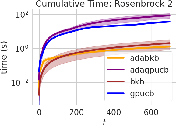
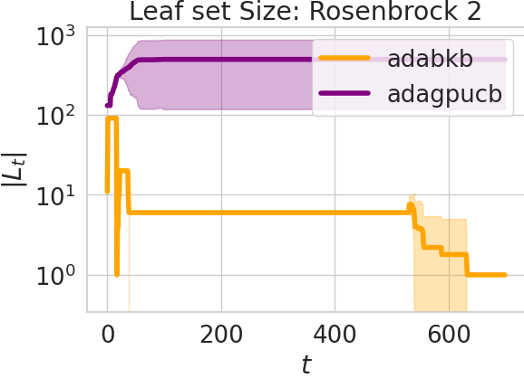
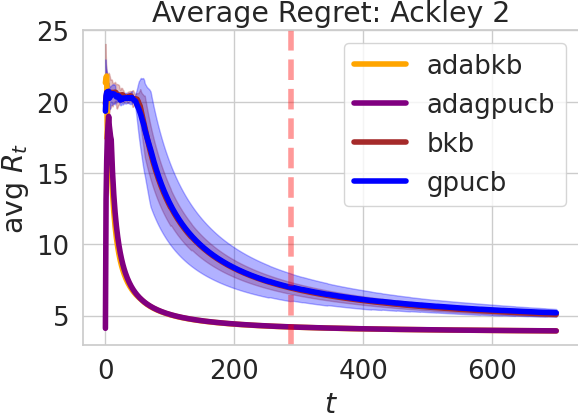
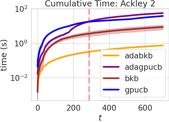
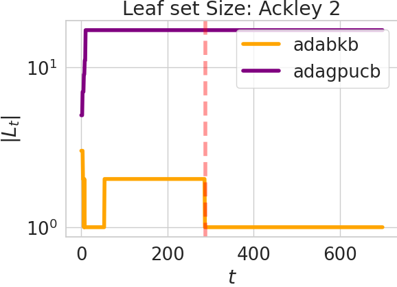
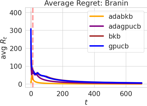
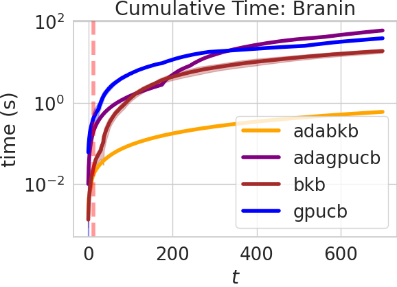
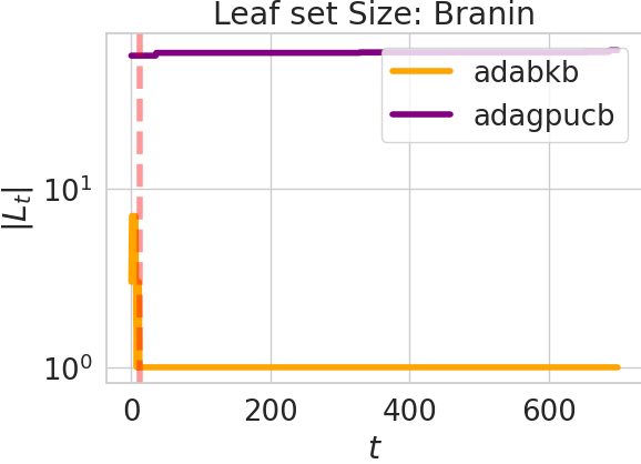
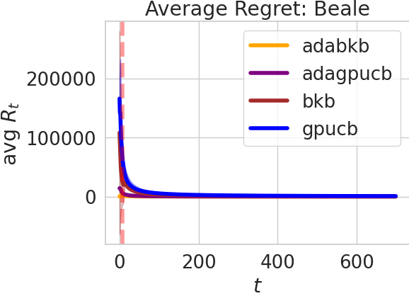
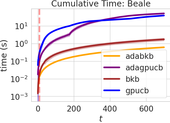
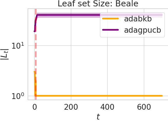
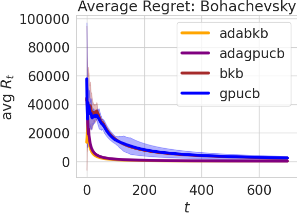
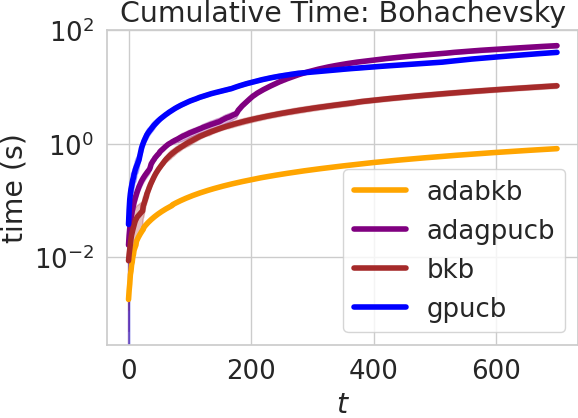
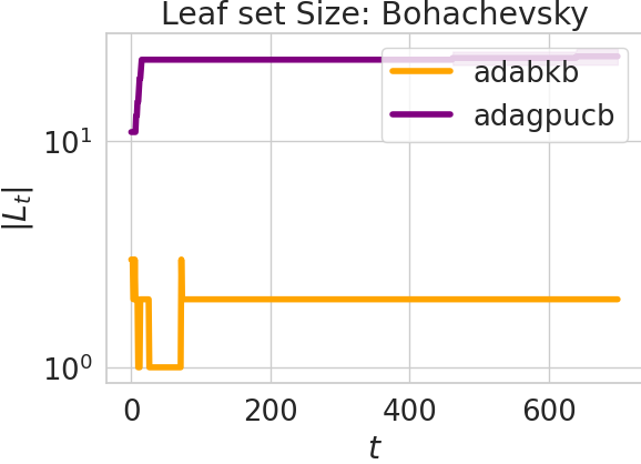
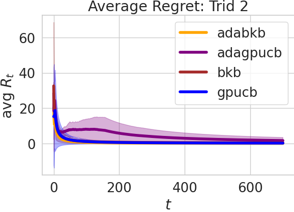
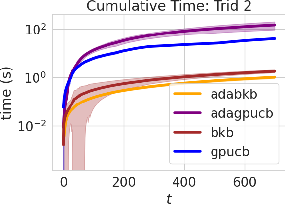
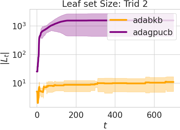
Figure 7: Average regret obtained by the algorithms in optimizing functions in Table 4

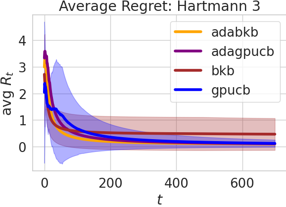
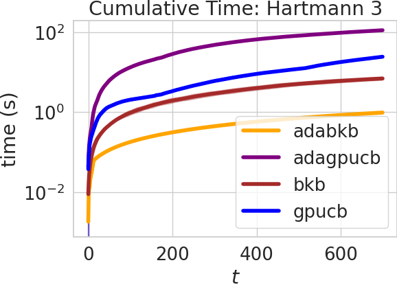
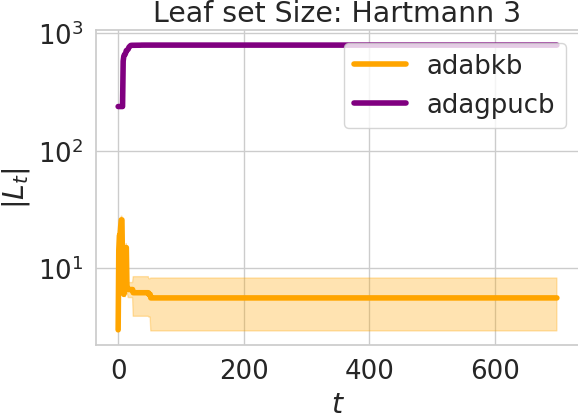
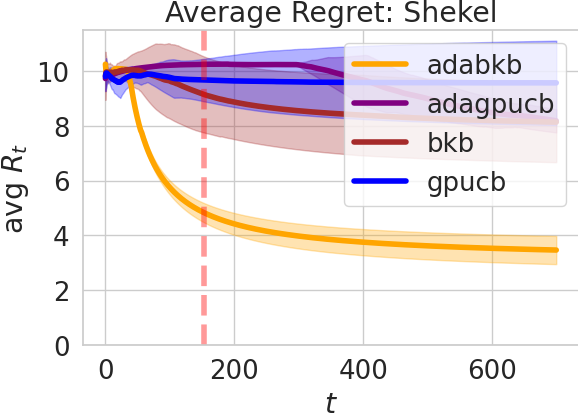
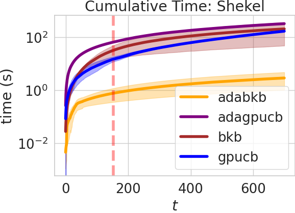
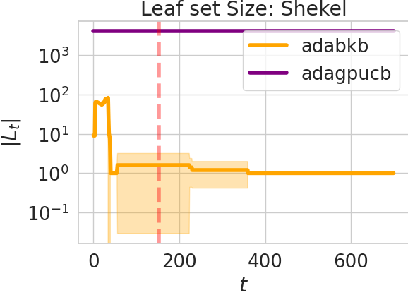
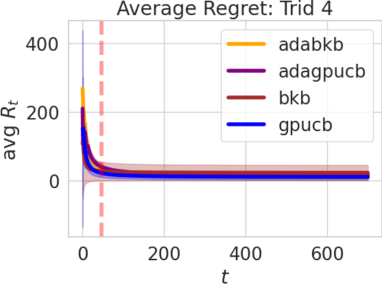
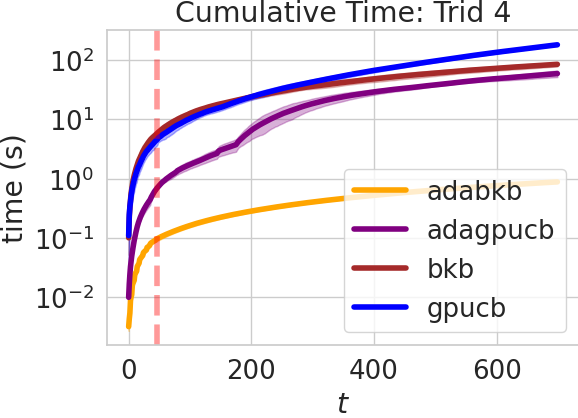
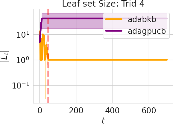
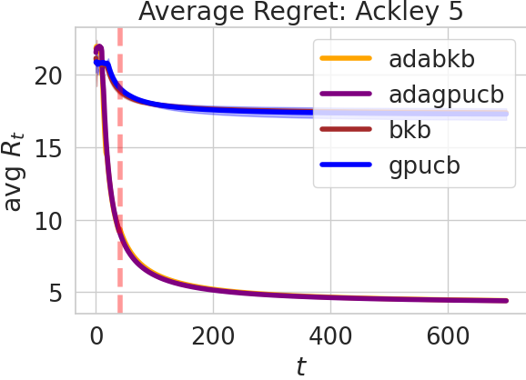
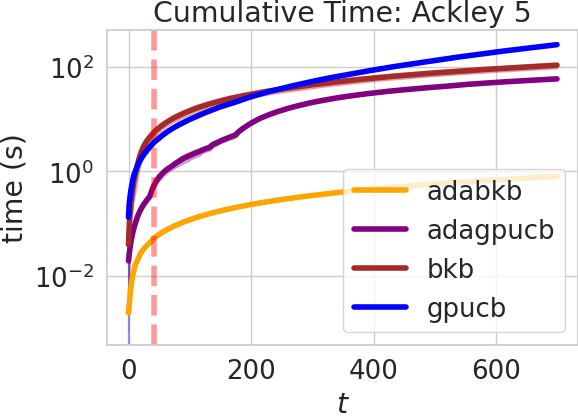
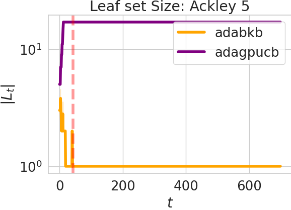
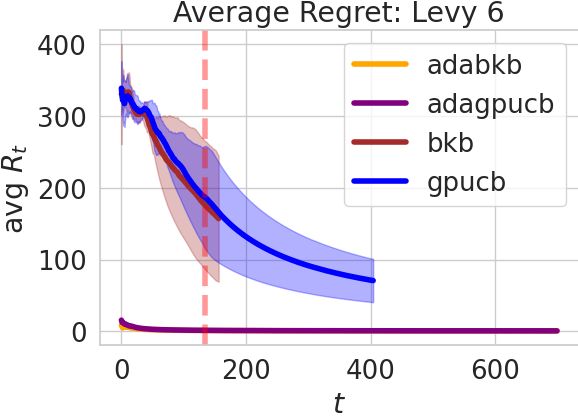
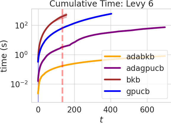
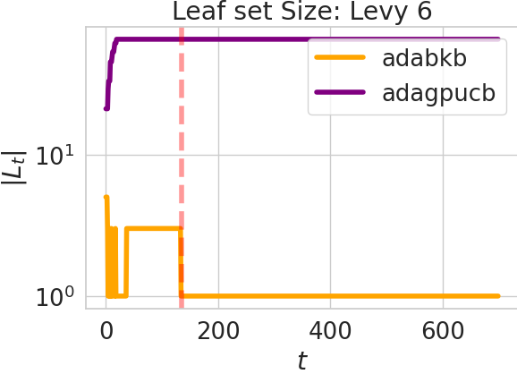
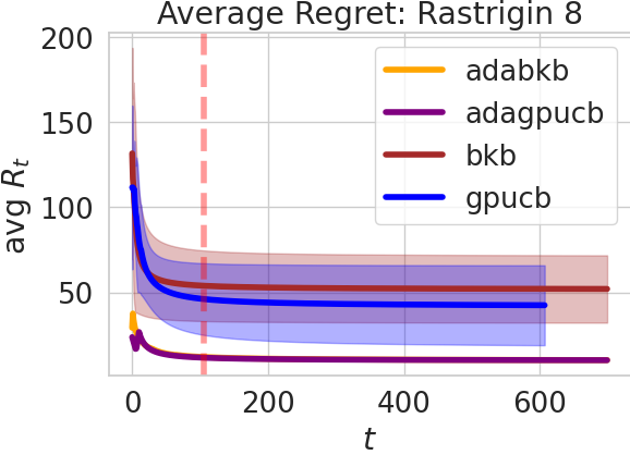
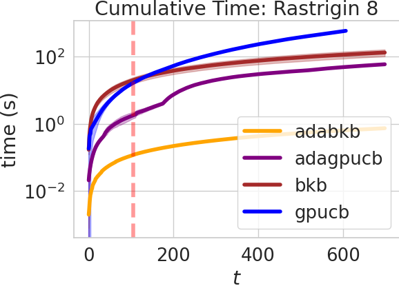
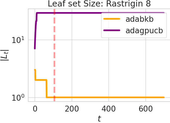
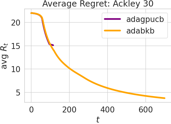
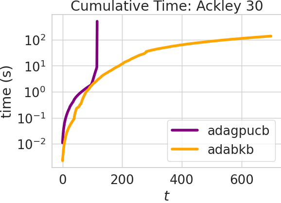
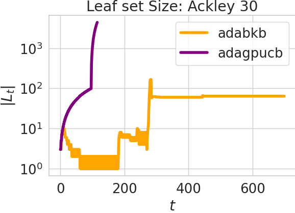
Figure 8: Average regret obtained by the algorithms in optimizing functions in Table 4

As in Section 5, we plot the average regret, cumulative time and leaf set size per iteration (Figure 7 and 8). As we expected, (in general) in low dimensional cases GP-UCB is faster than AdaGP-UCB because the discretization is composed of few points so the computations are fast and convergency is reached in few iterations. In Ada-BKB this problem is faced with the pruning procedure which reduces the number of nodes i.e. the number of points in which we have to evaluate the index function. In case the number of pruned nodes is $0$ we could expect that in low dimensional cases BKB is faster than Ada-BKB (notice in Rosenbrock 2 case that Ada-BKB achieves cumulative time similar to BKB and that the number of the pruned node during iteration is lower than the other low dimensional cases). However, we can notice that in these cases Ada-BKB is less time expensive than GP-UCB and Ada-GP-UCB. In the worst-case observed, it is similar (in time) to BKB.
Increasing the dimension of the search space (for instance in Ackley 5), Ada-BKB and AdaGP-UCB are faster than GP-UCB and BKB, and also the optimum found is better (according to the average regret). In the last line of Figure 8, we couldn’t realize the experiments for BKB and GP-UCB because the time cost was too high. Moreover, we can observe that in a $30$-dimensional case, AdaGP-UCB is interrupted due to the time threshold while Ada-BKB is able to complete the $700$ time steps. In general, we observe that AdaGP-UCB expands more than Ada-BKB because in AdaGP-UCB there is no pruning procedure (and probably because a different expression of $V_{h}$ is used) which reduce the number of nodes allowing to obtain a better performance in time.

C.5 Robustness to small pertubation of F

Since the choice of $F=1$ is an heuristic, we did some synthetic experiments comparing performances of Ada-BKB with different values for $F$.

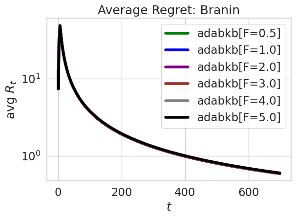
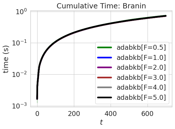
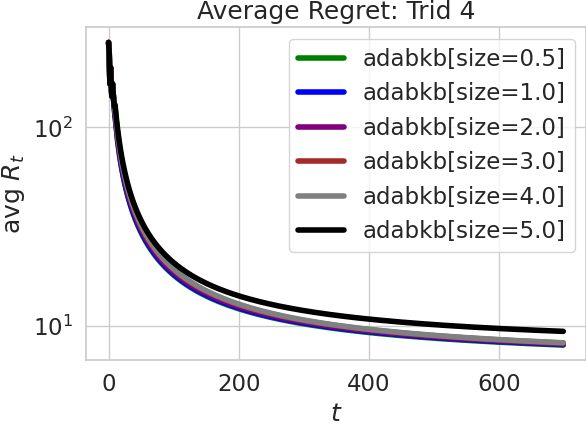
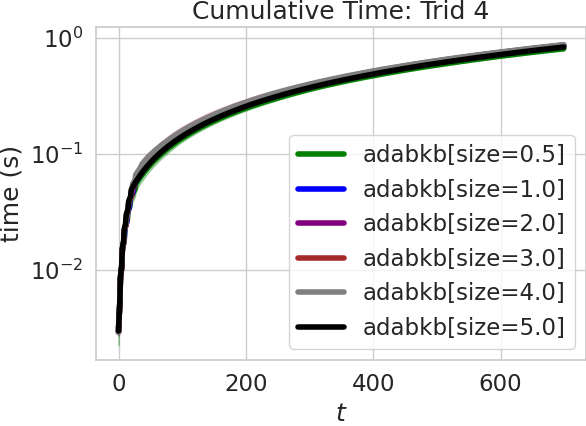
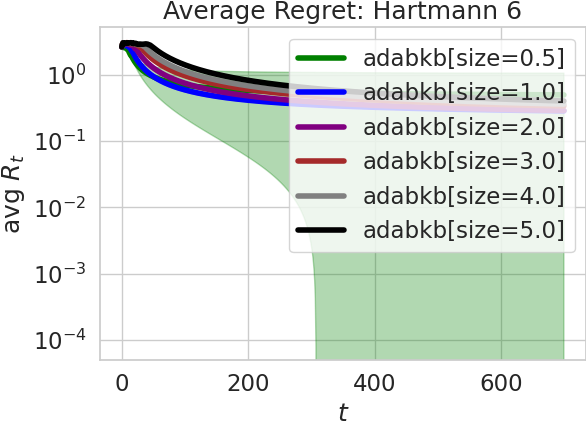
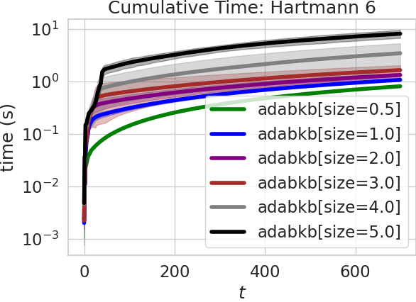
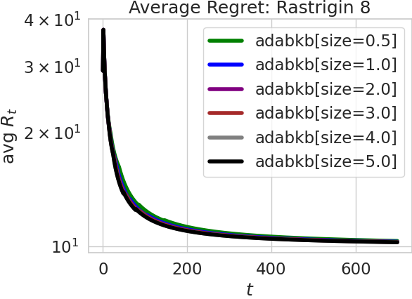
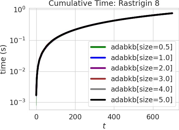
Figure 9: Average regret and cumulative time of Ada-BKB changing $F$

We can observe that for small changes of $F$, results in regret and time are similar i.e. the algorithm is robust to small changes of $F$. Obviously, taking $F$ too small will lead to small values for $V_{h}$ (eq. (8)) and, thus, the algorithm can evaluate centroid more times because of the expansion rule. On the other hand, taking $F$ too high can lead to over-expansion.

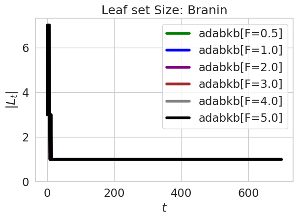
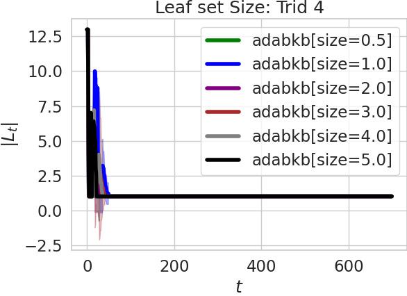
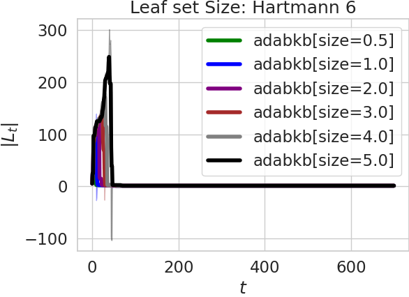
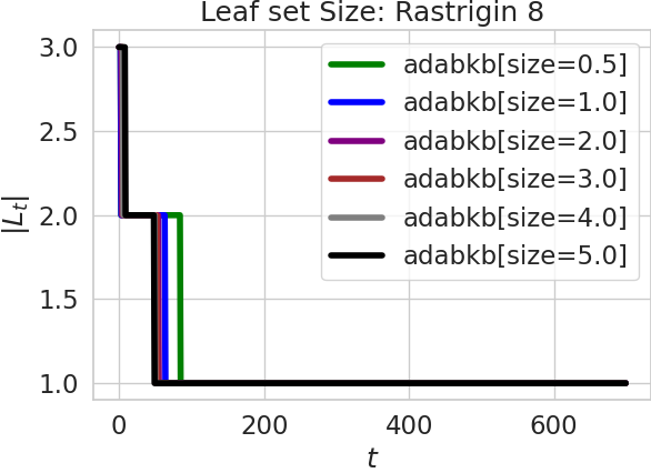
Figure 10: Leaf set size per iteration of Ada-BKB changing $F$

C.6 Partition tree selection

In practice, to run Ada-BKB, we have to choose the number of children per node $N$ (see Algorithm 1). The choice of a value for this parameter let us choose a partition tree used and explored as indicated in Section 3. Main results (see Section 4) suggest to choice this parameter as small as possible (i.e. $2$ or $3$) since it affects both computational cost and cumulative regret.

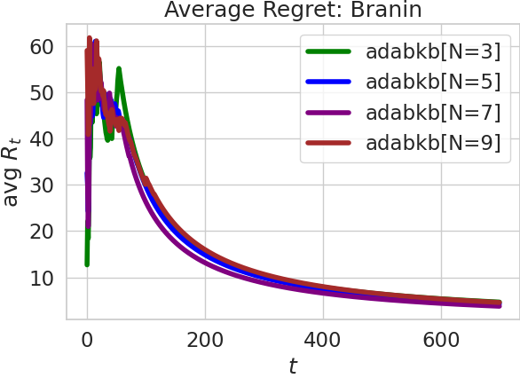
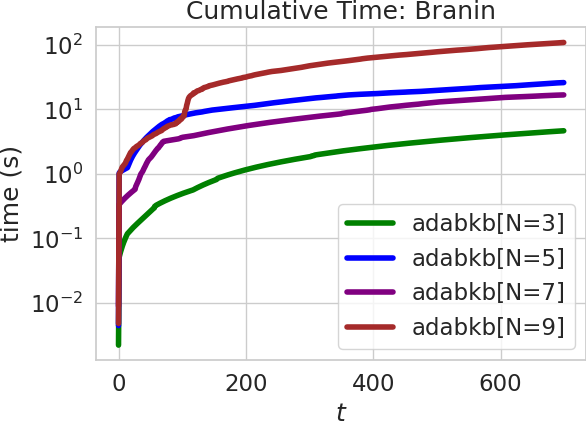
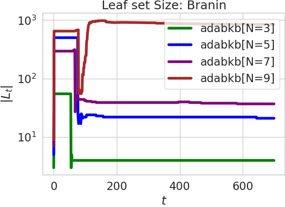
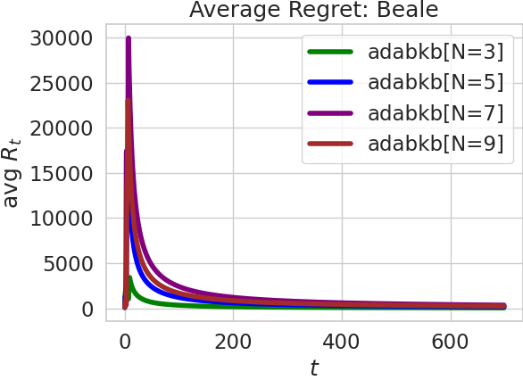
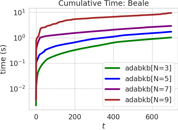
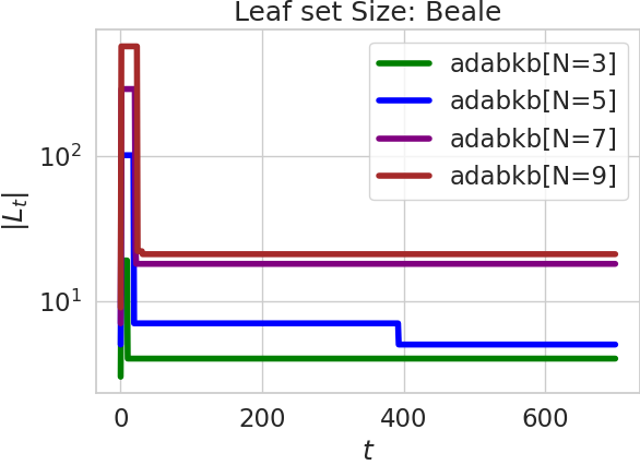
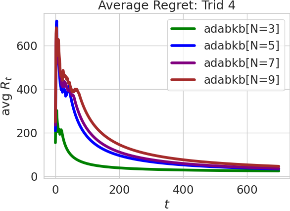
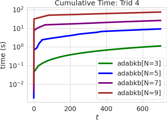
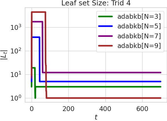
Figure 11: Average regret, cumulative time and leaf set size per iteration of Ada-BKB changing $N$

Considering a scenario in which we have a depth threshold $h_{\text{max}}$ and a budget $T$ high enough, we can observe that the number of children per node $N$ doesn’t drastically change the best configuration found by the algorithm (see Figure 11). Obviously, increasing $N$ will require a higher execution time since the cardinality of the leaf set will increase faster. However, in scenarios in which $h_{\text{max}}$ is low and the search space is a large hypercube, an high number of children per node can be usefull. Indeed, an high $N$ allows to produce small partitions faster than small $N$ according to the splitting procedure (see Section 3). This let Ada-BKB to provide good performance in regret (in practice) even when the maximum depth threshold $h_{\text{max}}$ is low.

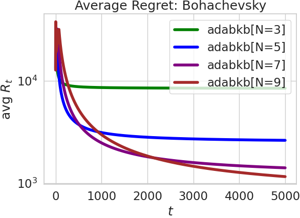
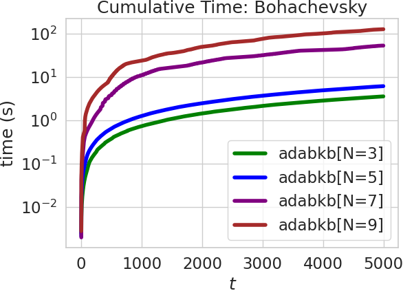
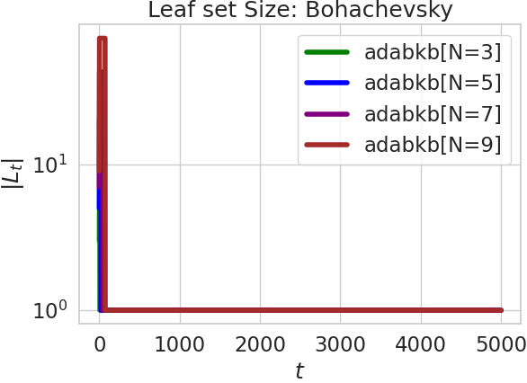
Figure 12: Average regret, cumulative time and leaf set size per iteration of Ada-BKB changing $N$ with $h_{\text{max}}=2$

In Figure 12, we optimize Bohachevsky function (see Appendix C for details on search space) with a maximum depth threshold $h_{\text{max}}=2$. In this case, we can observe that increasing $N$, we obtain better results in average regret but it decreases slower as expected (see Theorem 1). When we performed the experiments, we observed that a good way to select $N$ consists in starting with small values ($2$ or $3$) and increase it if the budget is large enough (which depends from the application), the search space is large and low-dimensional.

C.7 RandomBKB and Ada-BKB

To show the importance and the strength of adaptive discretizations, we compared Ada-BKB with BKB over a random discretization (called RandomBKB). The red vertical dashed line indicates when the early stopping condition is satisfied.

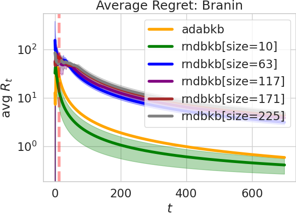
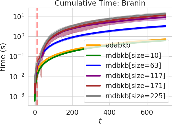
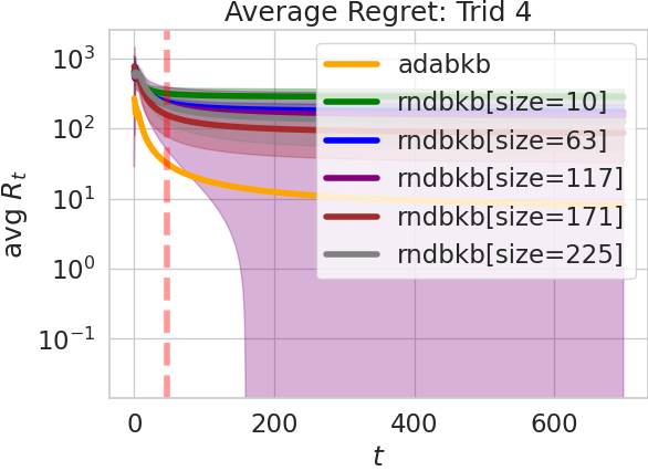
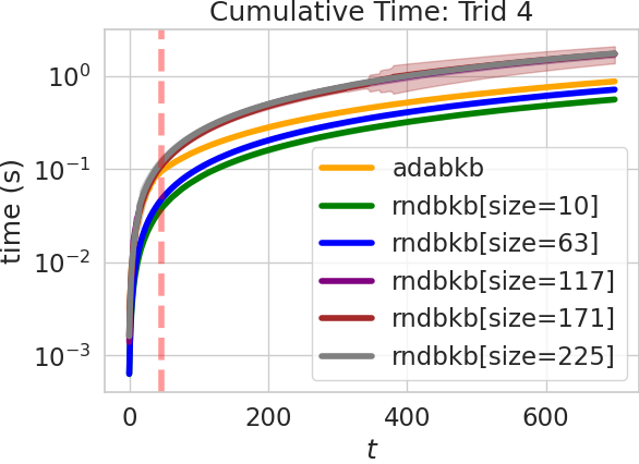
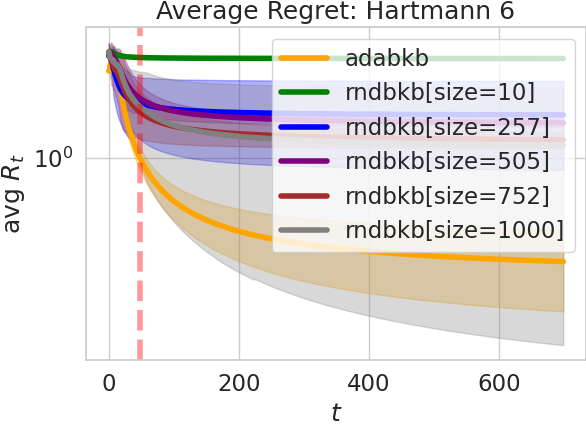
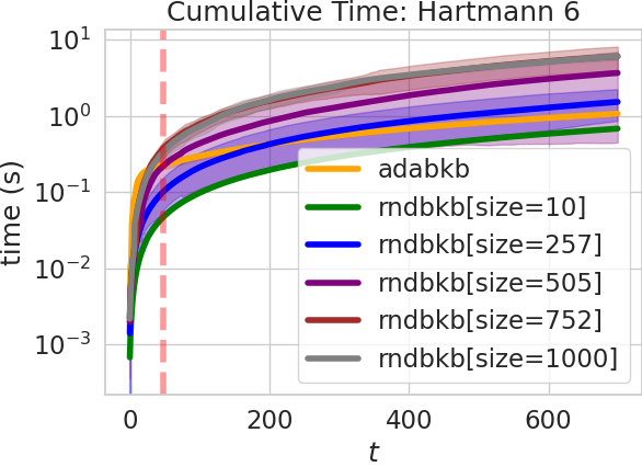
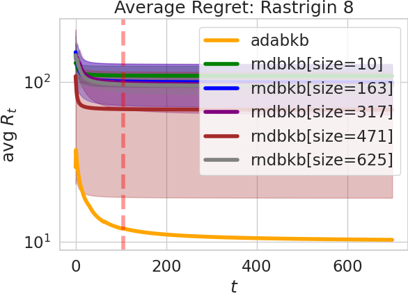
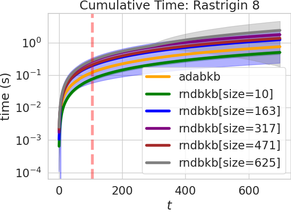
Figure 13: Average regret and cumulative time of Ada-BKB and RandomBKB with different discretization size

As we expected, in low dimensional case (Branin case) it is possible to build a random discretization which contains a sub-optimal configuration. Increasing the dimensions of the search space (as in Rastrigin 8 case), we can observe that even if we increase the size of discretizations used in RandomBKB, we still do not obtain results in regret as good as in Ada-BKB. This happens because in high dimensional cases the search space is too large and we need to generate many random points to have a good probability of obtaining a search space with suboptimal candidates. However, large discretizations, as we observed in Appendix C.4, will make BKB (and consequently also RandomBKB) very time-expensive due to the computations required to compute the posterior eq. (5) (indeed, obviously, we can notice that increasing the size of the random discretizations, the cumulative time spent to execute RandomBKB increases). Moreover, we can notice that Ada-BKB still achieves good performances in time and maintains (in mid and high dimensional search spaces) the best results in regret w.r.t. Random-BKB executions with lower variance (this because RandomBKB does not have a strategy to explore the search space, but it just builds random grids). This shows us that adaptive discretizations are more convenient than random discretizations.

C.8 Ada-BKB and GP-ThreDS

Ada-BKB parameters are indicated in Table 11. The implementation of GP-ThreDS used in these experiments can be downloaded from the official repository: https://github.com/sudeepsalgia/GP_ThreDS. The machine used to performe these experiments is less powerfull than the one described in Appendix C.3. We decided to use it in order to show that our algorithm can run and provide high performance also in low-powered machines. Details about this machine are reported in Table 12. We consider the same setting of Salgia et al., (2020) in which the Branin and Rosenbrock functions (defined in the same work) are optimized. As in Salgia et al., (2020), we will consider a search space $X=[0,1]^{2}$ for both functions. The hyperparameters used for GP-ThreDS are indicated in Salgia et al., (2020)[Appendix D.1]. The function evaluation budget is set to $T=700$.

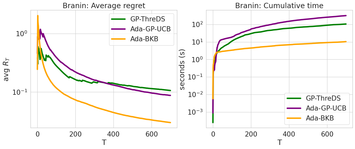
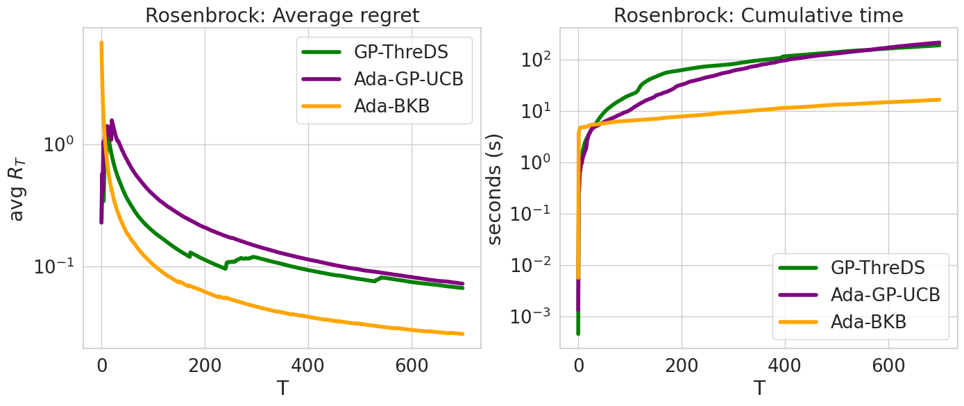
Figure 14: From left to right, average regret and cumulative time of Ada-BKB and GP-ThreDS in optimizing Branin and Rosenbrock functions.

As we can observe in Figure 14, Ada-BKB performs better than GP-ThreDS both in regret and cumulative time. Moreover, we can notice that GP-ThreDS performs better than Ada-GP-UCB in time but performs $\approx 10$ times worse than Ada-BKB (in computational time). In Table 10, we report the total time elapsed by three algorithms.

Table 10: Total time elapsed by algorithms to optimize Branin and Rosenbrock functions

ALGORITHM	BRANIN	ROSENBROCK
Ada-GP-UCB	318.65s	216.14s
GP-ThreDS	105.30s	190.17s
Ada-BKB	10.43s	16.56s

Table 11: Parameters of Ada-BKB algorithm to optimize Branin and Rosenbrock functions

FUNCTION	$\sigma$	$\lambda$	$F$	$N$	$h_{\text{max}}$
Branin	$0.5$	$0.001$	$1.0$	$3$	$7$
Rosenbrock	$0.5$	$0.001$	$1.0$	$5$	$5$

Table 12: Machine used to perform these experiments

FEATURE
OS	Debian 11
CPU	Intel(R) Core(TM) i7-8550U CPU 1.80GHz
RAM	16 GB

Appendix D EXPANDED DISCUSSION

In this appendix, we discuss the relationship of Algorithm 1 and the other similar recent algorithms. We focus to compare our Ada-BKB with GP-ThreDS (Salgia et al.,, 2020), AdaGP-UCB (Shekhar and Javidi,, 2018), LP-GP-UCB (Shekhar and Javidi,, 2020) and BKB (Calandriello et al.,, 2019). Despite BKB, our algorithm can work on continuous search spaces without building an offline discretization which can be very expensive, see Appendix C.4(notice that using random discretizations doesn’t provide good results in high-dimensional search spaces, see Appendix C.7). We followed the direction indicated in (Shekhar and Javidi,, 2020) to sketch the model confirming and proving that we get better performance in time. We also noticed that using a partition schema as in (Shekhar and Javidi,, 2018), let us obtain similar or potentially improved regret bounds with a lower computational cost:

$$(\text{LP-GP-UCB Regret:})\qquad\mathcal{O}(\sqrt{T}d_{\text{eff}}(T))$$

$$(\text{Ada-BKB Regret:})\qquad\mathcal{O}(\sqrt{T}d_{\text{eff}}(T)\log T)\qquad\text{or}\qquad\mathcal{O}\Bigg{(}\sqrt{Td_{\text{eff}}(T)\log T\frac{N^{h_{\text{max}}}-1}{N-1}}\Bigg{)}$$

Moreover, introducing a pruning procedure and an early stopping condition, we observed in the experiments (see Appendix C.4) that we can further reduce the time-cost in practice.

BKB and SVGP.

This work open other directions in particular in using different sketching models as SVGP (Titsias,, 2009; Burt et al.,, 2019) which mainly differs from BKB for inducing point selection. While in SVGP, inducing points are selected by maximizing the evidence lower bound (ELBO) (Hensman et al.,, 2015), BKB uses a procedure called resparsification which provides guarantees on the size of the set containing the inducing points (Calandriello et al.,, 2019, Theorem 1). Moreover, as shown in (Shekhar and Javidi,, 2018), using a Gaussian Process let us avoid to include in the $V_{h}$ expression (eq. (8)) the norm of the reward function $f$ which is not known a priori. In our experiments, we observed that a valid heuristic consists in setting it as $1$ (see also Appendix C.5).

Tuning the hyper-parameters of the model

As shown in (Wild et al.,, 2021; Calandriello et al.,, 2019), BKB is equivalent to a DTC approximation of a Gaussian Process (Quiñonero Candela and Rasmussen,, 2005) and thus, in practice, we can tune the hyper-parameters of BKB by maximizing the marginal likelihood.

References

- Bubeck et al., (2011) Bubeck, S., Munos, R., Stoltz, G., and Szepesvári, C. (2011). X-armed bandits. Journal of Machine Learning Research, 12:1655–1695.
- Buitinck et al., (2013) Buitinck, L., Louppe, G., Blondel, M., Pedregosa, F., Mueller, A., Grisel, O., Niculae, V., Prettenhofer, P., Gramfort, A., Grobler, J., Layton, R., VanderPlas, J., Joly, A., Holt, B., and Varoquaux, G. (2013). API design for machine learning software: experiences from the scikit-learn project. In ECML PKDD Workshop: Languages for Data Mining and Machine Learning, pages 108–122.
- Burt et al., (2019) Burt, D., Rasmussen, C. E., and Van Der Wilk, M. (2019). Rates of convergence for sparse variational Gaussian process regression. In Chaudhuri, K. and Salakhutdinov, R., editors, Proceedings of the 36th International Conference on Machine Learning, volume 97 of Proceedings of Machine Learning Research, pages 862–871. PMLR.