Evidence of many-body localization in 2D from quantum Monte Carlo simulation

Abstract

We use the stochastic series expansion quantum Monte Carlo method, together with the eigenstate-to-Hamiltonian construction, to map the localized Bose glass ground state of the disordered two-dimensional Heisenberg model to excited states of new target Hamiltonians. The localized nature of the ground state is established by studying the participation entropy, local entanglement entropy, and local magnetization, all known in the literature to also be identifying characteristics of many-body localized states. Our construction maps the ground state of the parent Hamiltonian to a single excited state of a new target Hamiltonian, which retains the same form as the parent Hamiltonian, albeit with correlated and large disorder. We furthermore provide evidence that the mapped eigenstates are genuine localized states and not special zero-measure localized states like the quantum scar-states. Our results provide concrete evidence for the existence of the many-body localized phase in two dimensions.

Introduction: Disorder and interactions induce novel phases and phenomena in quantum many body systems. Disordered non-interacting systems are known to have localized states in one and two dimensions Anderson (1958); Mott and Twose (1961); Gol’dshtein et al. (1977); Evers and Mirlin (2008). In recent years, it has emerged that localization of the entire eigenspectrum persists in the presence of interactions and strong disorder, constituting Many Body Localization (MBL) – a phenomenon that has been subject to intense investigation since its inception due to both fundamental and practical reasons  Basko et al. (2006); Nandkishore and Huse (2015). The MBL phase is a new phase of matter that breaks ergodicity and violates the Eigenvalue Thermalization Hypothesis (ETH) Nandkishore and Huse (2015); Alet and Laflorencie (2018); Abanin et al. (2019). In this phase, a closed system does not thermalize under its own dynamics, and hence cannot be described within the framework of conventional quantum statistical physics. At the same time, the long memory associated with the slow dynamics makes the MBL phase appealing for many practical applications Huse et al. (2013); Pekker et al. (2014); Bahri et al. (2015).

The existence of the MBL phase in one dimension has been well established through numerical Luitz et al. (2015); Serbyn and Moore (2016); Khemani et al. (2016); Lim and Sheng (2016) and analytical studies Imbrie et al. (2017) as well as in experiments Schreiber et al. (2015); Smith et al. (2016). On the other hand, its fate in two dimensions has been contentious De Roeck and Huveneers (2017); Doggen et al. (2020), though evidence is accumulating towards the affirmative Wahl et al. (2019); Kshetrimayum et al. (2020); Chertkov et al. (2021); Théveniaut et al. (2020); Decker et al. (2021). In this work, as shown in Fig. 1, we present convincing numerical evidence for the existence of MBL states in the 2D random-field Heisenberg antiferromagnet. Using the Eigenstate-to-Hamiltonian construction (EHC) described in  Chertkov and Clark (2018); Qi and Ranard (2019); Dupont and Laflorencie (2019), we map the Bose glass (BG) ground state obtained from large scale quantum Monte Carlo (QMC) simulations of the 2D disordered Heisenberg model to an excited state of another Hamiltonian that differs only in terms of the configuration of disorder (see Fig. 1 (a)). The state considered has non-ergodic properties characteristic of MBL states (see Fig. 1 (c)), while the new Hamiltonian has correlated disorder (Fig. 1 (b)). A crucial aspect of our work is the careful determination of the conditions of validity of this mapping. We also check that the obtained excited state is not a zero-measure non-ergodic state such as the many-body scar states Turner et al. (2018a); Serbyn et al. (2021) but a generic MBL state. This indicates the possibility of MBL states in 2D systems with correlated and large disorder.

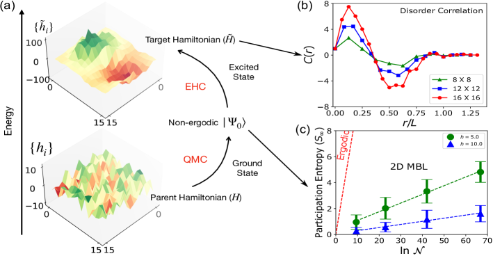
Figure 1: (a) Pictorial representation of our methodology to study many-body localization in 2D. The ground state, $|\Psi_{0}\rangle$, of a specified 2D parent Hamiltonian, ${\cal H}$, is obtained using QMC. The EHC is used to find a target Hamiltonians, $\tilde{\cal H}$, for which $|\Psi_{0}\rangle$ is an approximate excited eigenstate, allowing QMC to indirectly probe excited state properties. By construction both ${\cal H}$ and $\tilde{\cal H}$ exhibit the same form, and differ only in the local disorder distribution. The new disorder, $\{\tilde{h}_{i}\}$ is found to have a correlated structure, and to be of much larger strength than the original disorder, $\{h_{i}\}$, which is uncorrelated. (b) Averaged correlation function of the new disorder, $C(r)$ (see text) indicating strong spatial correlations of new disorder $\{\tilde{h}_{i}\}$. (c) Scaling of disorder-averaged participation entropy, $S_{\infty}$ of the state $|\Psi_{0}\rangle$ with the Hilbert space size, ${\cal N}$. The state exhibits non-ergodic behavior using metrics that are known in the literature (e.g. Ref. Macé et al. (2019)) to be identifying characteristics of many-body localization.

Background: There has been persistent controversy surrounding the existence of MBL in 2D. On one hand, the thermal avalanche argument states that rare regions of low disorder may form thermal bubbles that precipitate an avalanche effect, ultimately thermalising the system De Roeck and Huveneers (2017); Ponte et al. (2017); Doggen et al. (2020). However, later works have identified circumstances under which such avalanche events do not occur, or are not observable in an experimentally accessible time frame Potirniche et al. (2019); Foo et al. (2022). Moreover, the experimental signatures of the MBL are just as convincing in 2D as in 1D Schreiber et al. (2015); Choi et al. (2016); Bordia et al. (2016); Sbroscia et al. (2020).

From a computational perspective, establishing the existence of MBL in 2D is significantly more challenging than in 1D. Exact diagonalization (ED) is limited to system sizes that are generally too small to provide meaningful results (see however Théveniaut et al. (2020)). There is thus a need for approximate computational approaches that allow us to analyse highly excited states of disordered many-body systems. The main difficulty is that the density of high-energy states is exponentially large. Nevertheless, successful approximate methods have been developed, e.g. DMRG-X, shift-invert MPS and tensor network methods Khemani et al. (2016); Yu et al. (2017); Wahl et al. (2019).

A different line of study has emerged in recent years wherein one considers the ground state of interacting bosons or fermions with disorder (for which powerful numerical techniques exist in 2D and 3D) and then use the EHC formalism to identify a Hamiltonian for which the said ground state is an excited eigenstate. This was used in Refs.Dupont and Laflorencie (2019); Dupont et al. (2019) to study MBL in the 1D disordered Heisenberg model. Although MBL is a property of excited states, it shares several features in common with the ground state of disordered bosons; in particular, they both obey an area law for the entanglement entropy. The interplay between strong interactions and disorder in the ground state of interacting bosons has been extensively studied and results in the well-known BG phase, which is insulating and localized Giamarchi and Schulz (1987, 1988); Fisher et al. (1989a); Doggen et al. (2017).

This paper combines the versatility of established QMC methods with the recently proposed EHC to address the existence of MBL in 2D. The validity of the EHC is a very subtle question that we address carefully in this paper. It provides a way to use large scale numerical methods (such as QMC or DMRG) to address MBL properties, which are otherwise restricted to small system sizes. This is especially important in 2D. Furthermore, the EHC provides a way to systematically build Hamiltonians with MBL properties. The recent discovery of stark MBL and MBL by a confining potential suggest that non-trivial potentials/correlated disorders can induce MBL properties Schulz et al. (2019); Doggen et al. (2021); Yao et al. (2021); Foo et al. (2022). EHC provides a systematic way to build such Hamiltonians.

Model: The 2D $S=1/2$ antiferromagnetic Heisenberg model with random magnetic fields is described by the Hamiltonian,

$${\cal H}=\sum_{\langle i,j\rangle}{\bf S}_{i}\cdot{\bf S}_{j}+\sum_{i}h_{i}S_{i}^{z},$$ (1)

where ${\bf S}_{i}$ is the spin operator at site $i$, $\langle..\rangle$ indicates a sum over nearest-neighbour sites, and $h_{i}\in[-h,h]$ represents the local random magnetic field disorder. The Hamiltonian commutes with the total magnetization, $S^{z}_{\text{tot}}=\sum_{i}S_{i}^{z}$, – and only states in the $S^{z}_{\text{tot}}=0$ sector are considered when evaluating the ground state.

QMC-EHC method: We start by determining the ground state $|\Psi_{0}\rangle$ of ${\cal H}$, Eqn. (1), the parent Hamiltonian, using the stochastic series expansion (SSE) QMC method Sandvik (1992, 1999); Sengupta and Haas (2007). This method has been successfully used in the past to probe the superfluid to BG transition Fisher et al. (1989b); Pollet et al. (2009); Prokof’ev and Svistunov (2004); Álvarez Zúñiga et al. (2015). Due to the presence of a finite-size gap, the ground state can be accessed in SSE QMC by using a sufficiently large inverse temperature $\beta$  Prokof’ev and Svistunov (2004); Álvarez Zúñiga et al. (2015). In our simulations, we have set $\beta=8L$ to ensure we are in the ground state.

Next we conduct a search for a new Hamiltonian, $\tilde{{\cal H}}$, with the same form as ${\cal H}$ as in Eqn. (1), but different disorder configuration, for which $|\Psi_{0}\rangle$ is an eigenstate Qi and Ranard (2019); Chertkov and Clark (2018). The target Hamiltonian, $\tilde{{\cal H}}$, is obtained by analyzing the quantum covariance matrix, ${\mathcal{C}}_{ij}$, which is defined in terms of the ground state expectation values of the local Hamiltonian operators of ${\cal H}$ as

$${\mathcal{C}}_{ij}=\langle{\mathcal{O}}_{i}{\mathcal{O}}_{j}\rangle-\langle{\mathcal{O}}_{i}\rangle\langle{\mathcal{O}}_{j}\rangle,$$ (2)

where ${\mathcal{O}}_{0}=\sum_{\langle i,j\rangle}S_{i}^{z}S_{j}^{z}$ and ${\mathcal{O}}_{i}=S_{i}^{z},\;\;i=1,\ldots,N$. The determination of ${\mathcal{C}}_{ij}$ requires new measuring techniques in the SSE QMC approach that we detail in the Supplementary Material.

A normalized eigenvector $(\tilde{J},h^{{}^{\prime}}_{1},...,h^{{}^{\prime}}_{N})$ of ${\mathcal{C}}_{ij}$ contains the parameters defining a target Hamiltonian $\tilde{\cal H}=\sum_{\langle i,j\rangle}{\bf S}_{i}\cdot{\bf S}_{j}+\sum_{i}\tilde{h}_{i}S_{i}^{z}$ where $\tilde{h}_{i}=h^{{}^{\prime}}_{i}/\tilde{J}$. The corresponding eigenvalue $e$ gives the variance of the energy of $|\Psi_{0}\rangle$ with respect to $\tilde{\cal H}$:

$$e/\tilde{J}^{2}=\langle\Psi_{0}|\tilde{\cal H}^{2}|\Psi_{0}\rangle-\langle\Psi_{0}|\tilde{\cal H}|\Psi_{0}\rangle^{2}\;.$$ (3)

A vanishing eigenvalue of ${\mathcal{C}}_{ij}$ thus signals that $|\Psi_{0}\rangle$ is an eigenstate of $\tilde{\cal H}$ with energy $E=\langle\Psi_{0}|{\tilde{\cal H}}|\Psi_{0}\rangle$.

Working with an ordered set of eigenvalues, $e_{1},e_{2},\ldots,e_{N+1}$, of ${\mathcal{C}}_{ij}$, we note that the first two eigenvalues, $e_{1}$ and $e_{2}$ are always zero (up to numerical precision) - these correspond to the parent Hamiltonian, ${\cal H}$ and the constraint $S^{z}_{\text{tot}}=0$. The other eigenvalues $e_{j}$, $j>2$ will typically not be exactly zero. Nevertheless, a sufficiently small $e_{j}$ can still be used to define a target Hamiltonian, of which the ground state $|\Psi_{0}\rangle$ will be an approximate eigenstate. In the following, we focus on the smallest non-zero eigenvalue $e_{3}$. Our methodology is summarized in Fig. 1(a).

Bose glass ground state with characteristic non-ergodic properties of MBL states: Our model Eq. (1) has a Bose glass ground state beyond a certain critical disorder strength $h_{c}\approx 2.35$, see Álvarez Zúñiga et al. (2015) and Sup. Mat. We first show that this ground state has three distinct non-ergodic properties which are characteristic of MBL states.

We first consider the participation entropy (see Humeniuk and Roscilde (2012a); Luitz et al. (2014a, b) and Sup. Mat. for details of the calculation) which describes the contribution of basis states to the ground state wave function. In Fig. 1(c), we show the behavior of the disorder-averaged $S_{\infty}=\lim_{q\to\infty}\frac{1}{1-q}\ln\left(\sum_{i}|\langle\Psi_{0}|\phi_{i}\rangle|^{2q}\right)$, (where $|\phi_{i}\rangle$ are basis states) with the Hilbert space volume ${\cal N}$. We observe that $S_{\infty}=D\ln{\cal N}+c$, where $D$ is a multifractal dimension and $c$ is a constant. We clearly find $D<1$ and $c>0$ which indicates that only a vanishing fraction of states of the configuration space contribute to the Bose glass ground state. This is a clear signature of non-ergodic behavior which has been found in the MBL phase, see Ref. Macé et al. (2019). This behavior is in marked difference with the ETH ergodic regime, where $D=1$ and $c<0$. Similar scaling behavior is also observed for the second order participation entropy, $S_{2}$ (see Sup. Mat.).

Second, we measure the local entanglement entropy $S^{E}=-\ln\text{Tr}\rho_{loc}^{2}$ for a bipartition of the system as one site and the rest, using the SSE extended ensemble scheme Humeniuk and Roscilde (2012a); Luitz et al. (2014a, b). In Fig. 2(a), the distribution of $S^{E}$, $P(S^{E})$ shows a sharp peak close to $S^{E}=0$. This is a prominent feature of MBL (see Ref. Wahl et al. (2019)), where any given site is almost disentangled from other sites of the lattice and its reduced density matrix, $\rho_{\text{loc}}$ can be approximated as that of a pure state.

Third, in Fig. 2(b), we show the distribution of local magnetization $P(m_{z})$. We find a bipolar distribution with peak values at $m_{z}=\pm 1/2$, a signature of polarization along the on-site disordered magnetic field. Following Refs. Dupont and Laflorencie (2019); Laflorencie et al. (2020), we further look into the maximum polarisation, defined as $\delta_{\rm min}=1/2-{\rm max}(|m_{z}^{i}|)$. We observe that the typical average of $\delta_{\rm min}$, $\delta_{\rm min}^{\rm typ}\propto L^{-\gamma}$, with $\gamma\sim 3.5$ for $h=5$ (see inset). This behavior is analogous to the freezing of local moments in the MBL phase Dupont and Laflorencie (2019); Laflorencie et al. (2020).

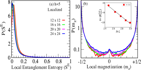
Figure 2: (a) Distribution of local entanglement entropy $P(S^{E})$ in the ground state for various system sizes for $h=5$. $P(S^{E})$ shows a sharp peak at $S^{E}\sim 0$ indicating that each site is almost disentangled from the other sites, a characteristic signature of MBL Wahl et al. (2019). As expected, the $S^{E}$ peak moves towards $S^{E}=0$ with increasing system sizes. (b) (Main panel) Distribution of local magnetization $P(m_{z})$ in the ground state for different system sizes for $h=5$. $P(m_{z})$ is strongly peaked at the values $m_{z}=\pm 1/2$, indicative of the local moments being fully aligned with the local random magnetic field. (Inset) Power-law decay of maximum polarization $\delta_{min}$ (see text) with system size, another characteristic signature of MBL Dupont and Laflorencie (2019); Laflorencie et al. (2020).

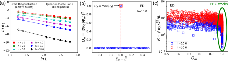
Figure 3: (a) Finite-size scaling of the disorder averaged energy variance, $\overline{e_{3}}$, obtained via ED and QMC methods. $\overline{e_{3}}$ exhibits a power law decay behavior with increased $L$. (b) Overlap of the true ground state, $|\Psi_{0}\rangle$, of $\cal H$ and a range of eigenstates of $\tilde{\cal H}$ close to $\tilde{E}$, obtained via ED with $4\times 4$ lattice. The overlap is maximum ($\approx 1$), for a single eigenstate with eigenvalue $\approx\tilde{E}$. This establishes that for sufficiently large disorder, EHC maps the ground state to a single excited eigenstate. (c) Comparison of relative residue, $R$ (see text) and maximum overlap, $O_{m}$, obtained from ED. EHC holds when $O_{m}\approx 1$, i.e. even for $R\gg 1$. In other words, the locality of MBL allows EHC to work, even if the energy resolution is not sufficient.

Reliability of EHC mapping: EHC is an approximate method and we here assess its reliability, see Fig. 3. We find that the disorder averaged $e_{3}$ decays as a power-law with system size, and thus vanishes in the thermodynamic limit (see Fig. 3(a)). This does not guarantee however that the ground state maps to a single eigenstate of the new Hamiltonian. In fact, as the excited states of a many-body system have an exponentially large density, the ground state could on the contrary correspond to a superposition of eigenstates. This limitation is common to all such approximate methods Khemani et al. (2016); Yu et al. (2017); Wahl et al. (2019).

To address this question, we use exact diagonalization Weinberg and Bukov (2017), keeping in mind the limited applicability to small system sizes (see Sup. Mat.). We determine the eigenstates $|\Psi_{\alpha}\rangle$ of ${\cal\tilde{H}}$ close in energy to that of the ground state $\tilde{E}=\langle\Psi_{0}|\tilde{\cal H}|\Psi_{0}\rangle$ and calculate their corresponding overlap $O_{\alpha}=|\langle\Psi_{0}|\Psi_{\alpha}\rangle|^{2}$. In Fig. 3(b), we observe that the maximum overlap, $O_{m}={\rm max}(O_{\alpha})\to 1$, indicating that for strong enough disorder, the ground state maps to a single eigenstate of ${\cal\tilde{H}}$.

An alternate figure of merit, accessible to QMC, is the relative residue, $R=\sqrt{e_{3}/\tilde{J}^{2}}/\Delta_{L}$, with $\Delta_{L}$ the mean level-spacing of the many-body Hamiltonian. Comparison of $R$ with $O_{m}$ is shown in Fig. 3(c). We clearly see that when $R<1$, i.e. when the error on the energy is small compared to $\Delta_{L}$, $O_{m}\approx 1$, thus the EHC works. However, we also observe that $O_{m}\approx 1$ for many realizations where $R\gg 1$. In other words, even if the energy resolution is not sufficient, the locality of MBL nevertheless allows EHC to work. This is a consequence of the non-ergodicity of the state $|\Psi_{0}\rangle$ and of the MBL properties of the new Hamiltonian (see below). Indeed, MBL states close by in energy are located far apart in configuration space. This is confirmed by the fact that EHC works better for larger disorder as seen in Fig. 3(c).

Properties of the new disorder: Unlike the original disorder which is uncorrelated, the new disorder $\tilde{h}_{i}$, obtained from EHC, is strongly correlated and of large amplitude. Similar to Refs. Dupont and Laflorencie (2019); Dupont et al. (2019), we observe that $\tilde{h}_{i}=h_{i}+\Delta h_{i}$, with $\Delta h_{i}$ showing strong spatial correlations of large amplitude. This is characterized by the disorder-averaged correlation function, $C(r)=(\sum_{d_{ij}=r}\Delta h_{i}\Delta h_{i+r})/(\sum_{i}\Delta h_{i}^{2})$, where $d_{ij}$ is the distance between sites $i$ and $j$. In fig. 1(b), we show the behavior of $C(r)$, where the correlation length is seen to vary like $L$, a signature of strong spatial correlations. Such spatial correlations can enhance MBL, similar to what has been seen in stark MBL Schulz et al. (2019); Doggen et al. (2021); Foo et al. (2022); Agrawal et al. (2022).

MBL properties of other eigenstates : There still exists a possibility that the mapped state is a zero-measure localized state, for example a quantum scar state, and not a genuine MBL eigenstate. To address this, we use ED calculations to study the localization properties of other eigenstates ($|\Psi_{\alpha}\rangle$) close by in energy to $\tilde{E}$. The inverse participation ratios ${\rm IPR}(\Psi_{\alpha})=\sum_{i}|\langle\Psi_{\alpha}|\phi_{i}\rangle|^{4}$ of these eigenstates Visscher (1972) are shown in fig. 4. They all have similar values as that of the mapped excited state, and therefore similar localization properties. This is in stark contrast with the case of the PXP model which is known to host quantum scar states Sun and Robicheaux (2008); Turner et al. (2018a, b) (see inset of fig. 4). This leads us to claim that the mapped states obtained via EHC approach belong to a genuine MBL phase.

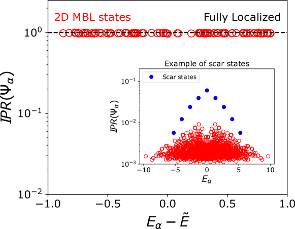
Figure 4: (Main panel) IPR of other eigenstates of $\tilde{\cal H}$ close by in energy to the mapped excited state, using ED on a $4\times 4$ lattice for $h=10$. The states exhibit similar IPR values and therefore similar localization properties. (Inset) Similar analysis for the $S=1/2$ PXP model on a chain of size $L=16$ which is known to host quantum scar-states Sun and Robicheaux (2008); Turner et al. (2018a, b). IPR values of the scar-states (blue filled circles) are orders of magnitude larger than those of the remaining eigenstates (red empty circles).

Conclusions: We have developed a new method for determining highly excited states of strongly disordered Hamiltonians of large sizes. This method, based on a combination of Quantum Monte Carlo and the Eigenstate to Hamiltonian Construction, allows us to map a ground state to a new Hamiltonian having this state as an approximate eigenstate. Applied to the disordered Heisenberg model, this method allows us to overcome the strong finite-size constraints encountered in numerical studies of MBL and to characterize MBL in two dimensions. At strong disorder, the Bose glass ground state has non-ergodic properties characteristic of MBL states, and we have carefully determined the conditions for this state to correspond to a unique excited state of the new constructed Hamiltonian. This new Hamiltonian retains the same form as the parent Hamiltonian, albeit with a correlated and large disorder. Furthermore, we have provided evidence that the mapped eigenstate is a genuine localized state and not a special zero-measure localized state like quantum scar-states.

Our work thus indicates the possibility of MBL states in 2D in systems where the disorder is strong and correlated. 2D MBL has been much debated recently, with some numerical Wahl et al. (2019); Kshetrimayum et al. (2020); Chertkov et al. (2021); Théveniaut et al. (2020); Decker et al. (2021) and experimental Choi et al. (2016); Bordia et al. (2016); Sbroscia et al. (2020) observations, but theoretical arguments exist that suggest it is unstable De Roeck and Huveneers (2017); Doggen et al. (2020). However, in the presence of correlations, as in stark MBL or with a quasiperiodic or confining potential, there seems to be a consensus in favor of a 2D MBL Schulz et al. (2019); Doggen et al. (2021); Foo et al. (2022); Agrawal et al. (2022). Our results both confirm this but moreover indicate how to systematically construct Hamiltonians with non-ergodic states, a very interesting possibility for applications in quantum technologies where non-ergodicity protects quantum information.

Supplementary Material

I Calculation of the Quantum Covariance Matrix with SSE QMC

The eigenstate to Hamiltonian construction (EHC) approach requires only a collection of expectation values with respect to the ground state in order to construct the quantum covariance matrix. In SSE QMC Sandvik et al. (1997); Sandvik (1999), ground state expectation values for finite size systems is obtained by choosing a sufficiently large inverse temperature $\beta$ (that depends on the system size). The spectrum of any finite-sized system is discrete and for simulations performed at temperatures smaller than the finite-size gap (between the ground state and the first excited state), contributions from higher energy states are exponentially suppressed, yielding ground state expectation values for the finite size system. Estimates for thermodynamic quantities are then obtained through a simultaneous finite-size and finite-temperature scaling (the temperature for each simulation is adjusted carefully to ensure that it is smaller than the finite size gap). In the literature, this approach has been successfully applied by all finite-temperature QMC algorithms (SSE, determinant QMC, world line QMC, path integral QMC) to investigate the ground state phases of interacting spins, bosons and fermions, both with and without disorder. In our simulations, we have set $\beta=8L$ to ensure we are in the ground state.

We calculate the quantum covariance matrix, $\bm{{\cal C}}$ with the SSE QMC method as follows. In the Hamiltonian of the 2D $S=1/2$ antiferromagnetic Heisenberg model considered

$${\cal H}=J\sum_{\langle i,j\rangle}{\bf S}_{i}\cdot{\bf S}_{j}+\sum_{i}h_{i}S_{i}^{z},$$ (4)

the Ising term ($S_{i}^{z}S_{j}^{z}$) and the magnetic field term ($h_{i}S_{i}^{z}$) are the diagonal terms ${\mathcal{O}}^{d}$, while the exchange term ($S_{i}^{x}S_{j}^{x}+S_{i}^{y}S_{j}^{y}$) is the off-diagonal term ${\mathcal{O}}^{od}$ Sandvik (2010). As described in the manuscript, the calculation of the covariance matrix involves the computation of expectation values of the product of terms of Eqn.(4). In SSE QMC, we use the Taylor expansion to expand the exponential part of the partition function. The partition function hence can be written as a sum of different Hamiltonian operators with the inverse temperature $\beta$ as its order, in which its sequence is usually referred to operator string.

I.1 ${\mathcal{O}}^{d}{\mathcal{O}}^{d}$ terms

As both of the terms belong to diagonal type operation, we can do direct measurement for every spin state along the non-empty operator string.

$$\langle{\mathcal{O}}^{d1}{\mathcal{O}}^{d2}\rangle=\big{\langle}\frac{1}{N_{H}}\sum_{p=1}^{N_{H}}{\mathcal{O}}^{d1}_{p}{\mathcal{O}}^{d2}_{p}\big{\rangle},$$ (5)

where $N_{H}$ is the total number of the non-empty operator string in each measuring step, $p$ is the slice index, and $\big{\langle}...\big{\rangle}$ is the average of Monte Carlo steps. As the spin state only changes during the off-diagonal operation, we can boost the efficiency by bookkeeping spins on most of the sites.

I.2 ${\mathcal{O}}^{od}{\mathcal{O}}^{od}$ terms

Only the exchange-exchange term in $\bm{{\cal C}}$ belongs to this category. We cannot directly measure the off-diagonal term from the spin state. Instead, we use the number of appearance of the consecutive operators along the operator string to estimate its value.

$$\langle{\mathcal{O}}^{od1}{\mathcal{O}}^{od2}\rangle=\frac{1}{\beta^{2}}\langle(N_{H}-1)N_{cons.}({\mathcal{O}}^{od1},{\mathcal{O}}^{od2})\rangle$$ (6)

where $N_{cons.}$ is the number of consecutive appearances of ${\mathcal{O}}^{od1}$ and ${\mathcal{O}}^{od2}$ along the operator string in each Monte Carlo step.

I.3 ${\mathcal{O}}^{d}{\mathcal{O}}^{od}$ terms

To calculate the combination of both diagonal and off-diagonal terms, we can combine both mentioned technique. At the occasion that ${\mathcal{O}}^{od}$ appears, we measure the ${\mathcal{O}}^{d}$ using direct measurement on the spin state.

$$\langle{\mathcal{O}}^{d1}{\mathcal{O}}^{od2}\rangle=\frac{1}{\beta}\langle\sum_{{\mathcal{O}}_{p}={\mathcal{O}}^{od2}}{\mathcal{O}}^{d1}_{p}\rangle$$ (7)

where ${\mathcal{O}}_{p}={\mathcal{O}}^{od2}$ is the slice that the operator is off-diagonal.

II Eigenstate-to-Hamiltonian Construction (EHC) Approach

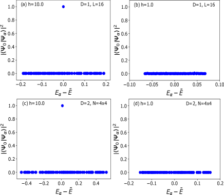
Figure 5: Figure highlighting the overlap of the ground state, $|\Psi_{0}\rangle$, of the parent Hamiltonian, ${\cal H}$, and the eigenstates of the mapped Hamiltonian, $\tilde{\cal H}$, close to the energy $\tilde{E}=\langle\Psi_{0}|\tilde{\cal H}|\Psi_{0}\rangle$, for a given disorder configuration of strength $h=10$ (left) and $h=1$ (right) in 1D (panels (a-b)) and 2D (panels (c-d)). As seen in the left panels, for large disorder value, the overlap is maximum ($\approx 1$) for a single eigenstate closest to $\tilde{E}$, indicating the EHC has successfully discovered a $\tilde{\cal H}$ hosting $|\Psi_{0}\rangle$ as an exact eigenstate. In contrast, for weak disorder (right panels), the overlap $\ll 1$, indicating a failure of the EHC.

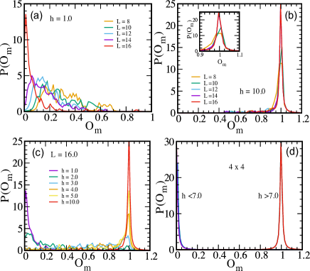
Figure 6: Distribution of the maximum overlap ($O_{m}$) of the ground state and the eigenstates of the mapped Hamiltonian, close to the energy $\tilde{E}$, for varying disorder strength and system sizes in 1D (panels (a)-(c)) and 2D (panel (d)). Panel (a) shows that for weak disorder values, the distribution of maximum overlap has a broad feature and a peak at vanishing overlap value for large system sizes. This indicates the mapping of the ground state to a superposition of eigenstates. Panel (b) shows that for large disorder value, the distribution of maximum overlap is peaked at $O_{m}\approx 1$. The peak strengthens with increasing system sizes, further establishing the fact the EHC mapping to only one eigenstate. The panel (c) shows this crossover behavior with gradually increasing/decreasing the disorder strength. In panel (d), we show this behavior for 2D, where we see a very sharp change in the behavior of the distribution of maximum overlap for weak and strong disorder values.

Once we have computed the quantum covariance matrix, we diagonalize it and label the eigenvalues in increasing magnitude as, $e_{1},e_{2},\ldots,e_{N+1}$. The first two eigenvalues, $e_{1}$ and $e_{2}$ are trivially zero, corresponding to the original parent Hamiltonian and the total spin operator. We consider the next non-zero eigenvalue, $e_{3}$ and the associated normalized eigenvector $\Psi_{3}=(\tilde{J},h^{{}^{\prime}}_{1},...,h^{{}^{\prime}}_{N})$ to construct the new Hamiltonian $\tilde{\cal H}$,

$$\tilde{\cal H}=\sum_{\langle i,j\rangle}{\bf S}_{i}\cdot{\bf S}_{j}+\sum_{i}\tilde{h}_{i}S_{i}^{z}$$ (8)

such that, $\tilde{h}_{i}=h^{{}^{\prime}}_{i}/\tilde{J}$. It can be shown that the variance $\sigma^{2}(\tilde{\cal H})=e_{3}/\tilde{J}^{2}$. Further, we show that disorder averaged $e_{3}$ exhibiting a power-law decay behavior with increased system size, thereby indicating that $|\Psi_{0}\rangle$ is an eigenstate of $\tilde{\cal H}$ with energy $\tilde{E}=\langle\Psi_{0}|\tilde{\cal H}|\Psi_{0}\rangle$ in the thermodynamic limit.

While the accuracy of the EHC mapping can be inferred from a decaying behavior of eigenvalues with increased system size, and thus vanishing in the thermodynamic limit, due to the exponentially large degeneracy of excited-eigenstates close to energy, $\tilde{E}$, the question remains, whether $\Psi_{0}$ maps to a single eigenstate of $\tilde{\cal H}$ or a superposition of eigenstates. We have performed Exact Diagonalization (ED) calculations in 1D and 2D, using the state-of-the-art Quspin packageWeinberg and Bukov (2017, 2019) to address this.

In Fig. 5, we show the overlap, $O_{\alpha}=|\langle\Psi_{0}|\Psi_{\alpha}\rangle|^{2}$ of the actual ground state, $\Psi_{0}$ and the eigenstates of the target Hamiltonian $\tilde{\cal H}$, close to the energy, $\tilde{E}=\langle\Psi_{0}|\tilde{\cal H}|\Psi_{0}\rangle$, for a single disorder realisation of strong and weak disorder values in a 1D chain of size $L=16$. We find that in the strong disorder case, the overlap is maximum $O_{m}\approx 1$ for a single eigenstate and vanishing for the remaining eigenstates. This indicates the EHC mapping to only one eigenstate in the strong disorder limit. On the other hand for the weak disorder configuration, the overlap is finite for several eigenstates. This is indicative of the fact that the ground state maps to a superposition of eigenstates. However, as the excited states are obtained from the mapping of the ground state, they have non-ergodic properties, which are quite interesting to study further. We observe a very similar feature in the overlap behavior for calculations in a 2D lattice of size $4\times 4$ (see bottom panels of Fig. 5).

Further, we study the distribution of the maximum overlap $O_{m}$ of the ground state and eigenstate of the mapped Hamiltonian, close to the energy, $\tilde{E}$, for representative weak ($h=1$) and strong ($h=10$) disorder values with varying system sizes in 1D. The distribution is computed for 5000 disorder configurations. As seen in Fig. 6, right panel, for large disorder value, the distribution is peaked at value $O_{m}\approx 1$. The peak strengthens with increasing system sizes, further establishing the fact that the ground state has overlap with a single eigenstate of the mapped Hamiltonian obtained via the EHC formalism. In contrast, for weak disorder (left panel), the distribution peaks for vanishing values of overlap for large system sizes. This indicates that the ground state has overlap with a superposition of eigenstates of the new Hamiltonian obtained via the EHC formalism. The bottom-left panel of Fig. 6 shows this crossover behavior with gradually increasing/decreasing the disorder strength. We show this behavior for 2D in the bottom-right panel of Fig. 6. We find that the distribution of the maximum overlap exhibits similar behavior for the 1D chain and the 2D lattice.

III Participation Entropy

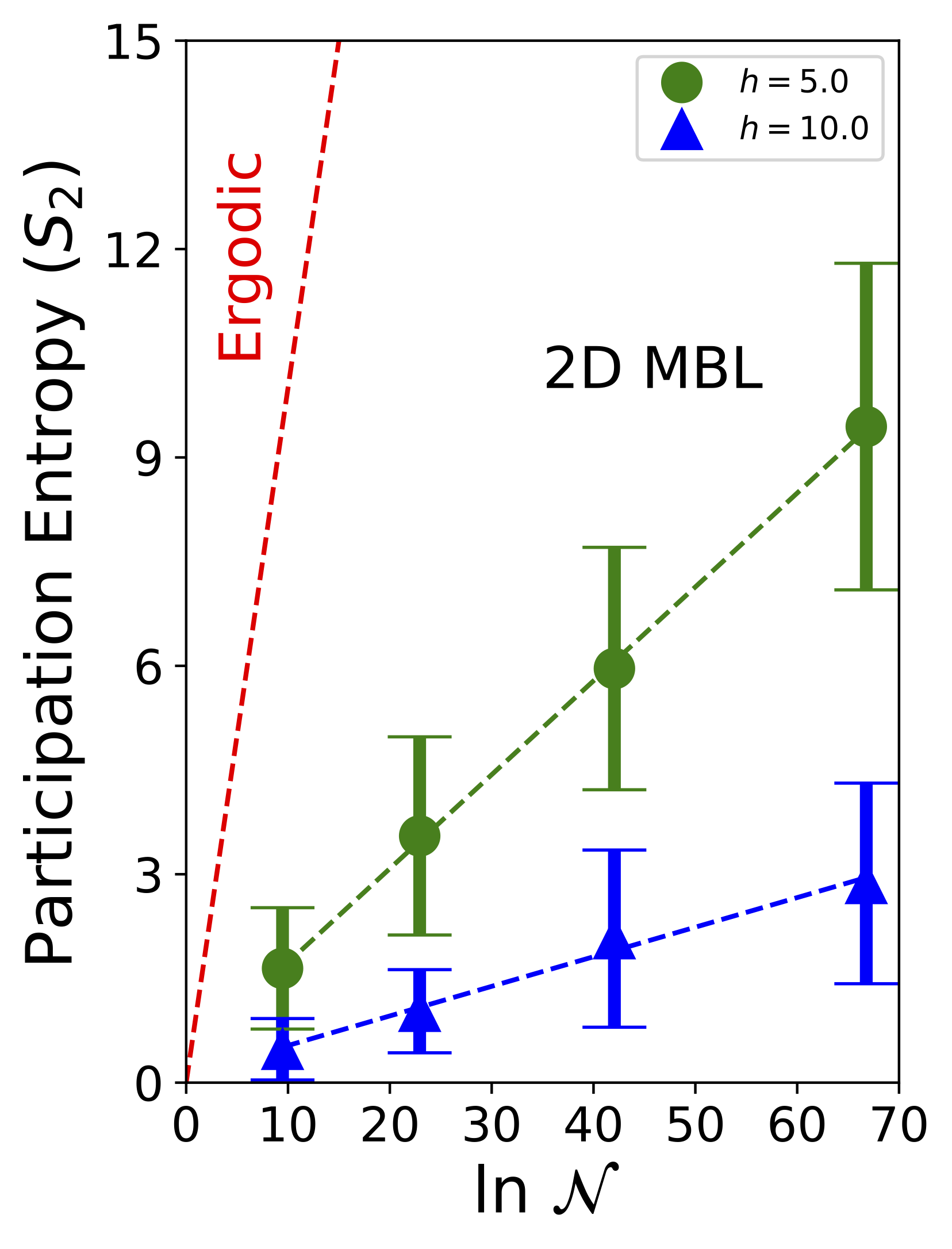
Figure 7: Scaling of second order Renyi entropy, $S_{2}$ with the Hilbert space size ${\cal N}$ in the presence of disorder, demonstrating the non-ergodic behavior of the Bose glass ground state.

The $q$-th order Rényi participation entropy of a state $\ket{\psi}$ is given by

$$S_{q}=\frac{1}{1-q}\ln\sum_{i}p^{q}_{i},$$ (9)

where $p_{i}=|\braket{\psi}{\phi_{i}}|^{2}$ and the $\ket{\phi_{i}}$ are some set of orthonormal basis states. In particular, we focus on $q=2$ and $q\to\infty$. These two quantities provide the measure of how many states of a configuration space contribute to a wave function.

We use the approaches developed in Humeniuk and Roscilde (2012b); Luitz et al. (2014c, b) to calculate the participation entropy. These approaches use the counting of occurrence for each spin configuration to calculate the participation entropy. $S_{q}$ is found using the probability of having identical configurations in different replica in each Monte Carlo step, while $S_{\infty}$ is calculated using the probability of maximally occurring spin configuration. For strong disorders, the maximally occurred spin configuration is usually almost aligned with the local magnetic field.

In Fig. 7, we show the scaling of disorder-averaged $S_{2}$ with the Hilbert space size, ${\cal N}$ in the localised regime. The slope of the line $S_{2}=D_{2}\ln{\cal N}+c$ represents the multifractal dimension $D_{2}$, and we find $D_{2}\ll 1$. This indicates that only a vanishingly small fraction of basis states (among the exponentially large space of states in the configuration space) contribute to the Bose glass ground state in our simulations; highlighting it’s strong non-ergodic behavior. The behavior of $S_{\infty}$ is shown in the main text.

IV Ground state phase transition

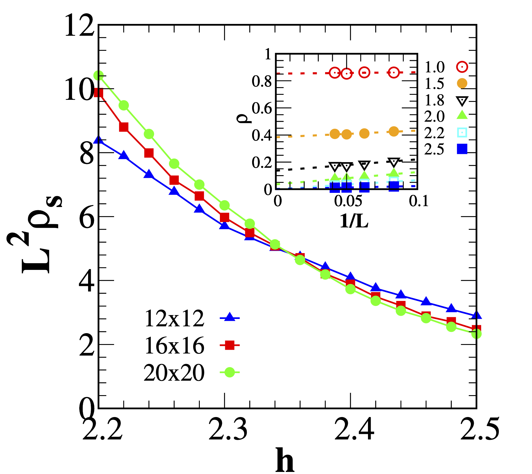
Figure 8: (Main) Behaviour of the scaled stiffness, $L^{2}\rho_{s}$, with varying $h$ near the transition region. The curves for different system sizes cross at $h=h_{c}$, providing an accurate estimate of the critical disorder strength, $h_{c}\approx 2.35$. (Inset) Finite size scaling of the spin stiffness, $\rho_{s}$, with varying system sizes for different disorder strengths. In the thermodynamic limit, $\rho_{s}\to 0$ as $h\geq h_{c}$ increases, establishing the BG phase as the ground state.

The ground state of ${\cal H}$, Eq. (4), has two distinct phases as disorder strength $h$ varies, with a quantum phase transition at a critical $h_{c}$. These phases may be characterised by measuring the spin stiffness, $\rho_{s}=\frac{1}{N}\frac{\partial^{2}E}{\partial\phi^{2}}$, defined as the response of the total energy, $E$, to a twist by angle $\phi$. The delocalized superfluid (SF) phase (for $h<h_{c}$) has finite spin stiffness, whereas the localized Bose glass (BG) phase (for $h>h_{c}$) has vanishing spin stiffness, and $h_{c}$, can be determined from the scaling of $\rho_{s}$.

In SSE, the stiffness is measured by the fluctuation in winding number($W$) of the world lines as $\rho_{s}=\langle W^{2}\rangle/2\beta$, where $\beta$ is the inverse temperature Sandvik (2010). Close to the critical point, the stiffness obeys the scaling relation

$$\rho_{s}(L,h)=L^{-z}f[(h-h_{c})L^{1/\nu}],$$ (10)

where the correlation length exponent is $\nu=1$ Prokof’ev and Svistunov (2004), and the dynamical critical exponent is found to be $z=2$. Plotting the scaled stiffness $L^{z}\rho_{s}$ against $h$ for different system sizes provides an accurate estimate of the critical disorder strength, $h_{c}$ Álvarez Zúñiga et al. (2015). The results are shown in Fig. 8, which suggest $h_{c}\approx 2.35$. The interacting ground state changes from a delocalized superfluid state to a localized Bose glass state for $h>h_{c}$.

References

- Anderson (1958) P. W. Anderson, Phys. Rev. 109, 1492 (1958).
- Mott and Twose (1961) N. Mott and W. Twose, Advances in Physics 10, 107 (1961).
- Gol’dshtein et al. (1977) I. Y. Gol’dshtein, S. A. Molchanov, and L. A. Pastur, Functional Analysis and Its Applications 11, 1 (1977).
- Evers and Mirlin (2008) F. Evers and A. D. Mirlin, Rev. Mod. Phys. 80, 1355 (2008).
- Basko et al. (2006) D. Basko, I. Aleiner, and B. Altshuler, Ann. Phys. (N. Y.) 321, 1126 (2006).
- Nandkishore and Huse (2015) R. Nandkishore and D. A. Huse, Annu. Rev. Condens. Matter Phys. 6, 15 (2015).
- Alet and Laflorencie (2018) F. Alet and N. Laflorencie, C. R. Phys. 19, 498 (2018).
- Abanin et al. (2019) D. A. Abanin, E. Altman, I. Bloch, and M. Serbyn, Rev. Mod. Phys. 91, 021001 (2019).
- Huse et al. (2013) D. A. Huse, R. Nandkishore, V. Oganesyan, A. Pal, and S. L. Sondhi, Phys. Rev. B 88, 014206 (2013).
- Pekker et al. (2014) D. Pekker, G. Refael, E. Altman, E. Demler, and V. Oganesyan, Phys. Rev. X 4, 011052 (2014).
- Bahri et al. (2015) Y. Bahri, R. Vosk, E. Altman, and A. Vishwanath, Nat. Commun. 6, 7341 (2015).
- Luitz et al. (2015) D. J. Luitz, N. Laflorencie, and F. Alet, Phys. Rev. B 91, 081103(R) (2015).
- Serbyn and Moore (2016) M. Serbyn and J. E. Moore, Phys. Rev. B 93, 041424(R) (2016).
- Khemani et al. (2016) V. Khemani, F. Pollmann, and S. L. Sondhi, Phys. Rev. Lett. 116, 247204 (2016).
- Lim and Sheng (2016) S. P. Lim and D. N. Sheng, Phys. Rev. B 94, 045111 (2016).
- Imbrie et al. (2017) J. Z. Imbrie, V. Ros, and A. Scardicchio, Annalen der Physik 529, 1600278 (2017).
- Schreiber et al. (2015) M. Schreiber, S. S. Hodgman, P. Bordia, H. P. Lüschen, M. H. Fischer, R. Vosk, E. Altman, U. Schneider, and I. Bloch, Science 349, 842 (2015).
- Smith et al. (2016) J. Smith, A. Lee, P. Richerme, B. Neyenhuis, P. W. Hess, P. Hauke, M. Heyl, D. A. Huse, and C. Monroe, Nat. Phys. 12, 907 (2016).
- De Roeck and Huveneers (2017) W. De Roeck and F. Huveneers, Phys. Rev. B 95, 155129 (2017).
- Doggen et al. (2020) E. V. H. Doggen, I. V. Gornyi, A. D. Mirlin, and D. G. Polyakov, Phys. Rev. Lett. 125, 155701 (2020).
- Wahl et al. (2019) T. B. Wahl, A. Pal, and S. H. Simon, Nat. Phys. 15, 164 (2019).
- Kshetrimayum et al. (2020) A. Kshetrimayum, M. Goihl, and J. Eisert, Phys. Rev. B 102, 235132 (2020).
- Chertkov et al. (2021) E. Chertkov, B. Villalonga, and B. K. Clark, Phys. Rev. Lett. 126, 180602 (2021).
- Théveniaut et al. (2020) H. Théveniaut, Z. Lan, G. Meyer, and F. Alet, Phys. Rev. Research 2, 033154 (2020).
- Decker et al. (2021) K. S. C. Decker, D. M. Kennes, and C. Karrasch, arXiv:2106.12861 (2021).
- Chertkov and Clark (2018) E. Chertkov and B. K. Clark, Phys. Rev. X 8, 031029 (2018).
- Qi and Ranard (2019) X. L. Qi and D. Ranard, Quantum 3, 159 (2019).
- Dupont and Laflorencie (2019) M. Dupont and N. Laflorencie, Phys. Rev. B 99, 020202(R) (2019).
- Turner et al. (2018a) C. J. Turner, A. A. Michailidis, D. A. Abanin, M. Serbyn, and Z. Papić, Nature Physics 14, 745 (2018a).
- Serbyn et al. (2021) M. Serbyn, D. A. Abanin, and Z. Papić, Nature Physics 17, 675 (2021).
- Macé et al. (2019) N. Macé, F. Alet, and N. Laflorencie, Phys. Rev. Lett. 123, 180601 (2019).
- Ponte et al. (2017) P. Ponte, C. R. Laumann, D. A. Huse, and A. Chandran, Philosophical Transactions of the Royal Society A: Mathematical, Physical and Engineering Sciences 375, 1 (2017).
- Potirniche et al. (2019) I. D. Potirniche, S. Banerjee, and E. Altman, Phys. Rev. B 99, 205149 (2019).
- Foo et al. (2022) D. C. W. Foo, N. Swain, P. Sengupta, G. Lemarié, and S. Adam, arXiv:2022.09072 (2022).
- Choi et al. (2016) J. Y. Choi, S. Hild, J. Zeiher, P. Schauß, A. Rubio-Abadal, T. Yefsah, V. Khemani, D. A. Huse, I. Bloch, and C. Gross, Science 352, 1547 (2016).
- Bordia et al. (2016) P. Bordia, H. P. Lüschen, S. S. Hodgman, M. Schreiber, I. Bloch, and U. Schneider, Phys. Rev. Lett. 116, 140401 (2016).
- Sbroscia et al. (2020) M. Sbroscia, K. Viebahn, E. Carter, J.-C. Yu, A. Gaunt, and U. Schneider, Phys. Rev. Lett. 125, 200604 (2020).
- Yu et al. (2017) X. Yu, D. Pekker, and B. K. Clark, Phys. Rev. Lett. 118, 017201 (2017).
- Dupont et al. (2019) M. Dupont, N. Macé, and N. Laflorencie, Phys. Rev. B 100, 134201 (2019).
- Giamarchi and Schulz (1987) T. Giamarchi and H. J. Schulz, Europhysics Letters (EPL) 3, 1287 (1987).
- Giamarchi and Schulz (1988) T. Giamarchi and H. J. Schulz, Phys. Rev. B 37, 325 (1988).
- Fisher et al. (1989a) M. P. A. Fisher, P. B. Weichman, G. Grinstein, and D. S. Fisher, Phys. Rev. B 40, 546 (1989a).
- Doggen et al. (2017) E. V. H. Doggen, G. Lemarié, S. Capponi, and N. Laflorencie, Phys. Rev. B 96, 180202(R) (2017).
- Schulz et al. (2019) M. Schulz, C. A. Hooley, R. Moessner, and F. Pollmann, Phys. Rev. Lett. 122, 040606 (2019).
- Doggen et al. (2021) E. V. H. Doggen, I. V. Gornyi, and D. G. Polyakov, Phys. Rev. B 103, L100202 (2021).
- Yao et al. (2021) R. Yao, T. Chanda, and J. Zakrzewski, Phys. Rev. B 104, 014201 (2021).
- Sandvik (1992) A. W. Sandvik, J. Phys. A: Math. Gen. 25, 3667 (1992).
- Sandvik (1999) A. W. Sandvik, Phys. Rev. B 59, R14157 (1999).
- Sengupta and Haas (2007) P. Sengupta and S. Haas, Phys. Rev. Lett. 99, 050403 (2007).
- Fisher et al. (1989b) M. P. A. Fisher, P. B. Weichman, G. Grinstein, and D. S. Fisher, Phys. Rev. B 40, 546 (1989b).
- Pollet et al. (2009) L. Pollet, N. V. Prokof’ev, B. V. Svistunov, and M. Troyer, Phys. Rev. Lett. 103, 140402 (2009).
- Prokof’ev and Svistunov (2004) N. Prokof’ev and B. Svistunov, Phys. Rev. Lett. 92, 015703 (2004).
- Álvarez Zúñiga et al. (2015) J. P. Álvarez Zúñiga, D. J. Luitz, G. Lemarié, and N. Laflorencie, Phys. Rev. Lett. 114, 155301 (2015).
- Humeniuk and Roscilde (2012a) S. Humeniuk and T. Roscilde, Phys. Rev. B 86, 235116 (2012a).
- Luitz et al. (2014a) D. J. Luitz, X. Plat, N. Laflorencie, and F. Alet, Phys. Rev. B 90, 125105 (2014a).
- Luitz et al. (2014b) D. J. Luitz, F. Alet, and N. Laflorencie, Phys. Rev. Lett. 112, 057203 (2014b).
- Laflorencie et al. (2020) N. Laflorencie, G. Lemarié, and N. Macé, Phys. Rev. Research 2, 042033(R) (2020).
- Weinberg and Bukov (2017) P. Weinberg and M. Bukov, SciPost Phys. 2, 003 (2017).
- Agrawal et al. (2022) U. Agrawal, R. Vasseur, and S. Gopalakrishnan, arXiv preprint arXiv:2204.03665 (2022).
- Visscher (1972) W. Visscher, Journal of Non-Crystalline Solids 8-10, 477 (1972).
- Sun and Robicheaux (2008) B. Sun and F. Robicheaux, New J. Phys. 10, 045032 (2008).
- Turner et al. (2018b) C. J. Turner, A. A. Michailidis, D. A. Abanin, M. Serbyn, and Z. Papić, Phys. Rev. B 98, 155134 (2018b).
- Sandvik et al. (1997) A. W. Sandvik, R. R. P. Singh, and D. K. Campbell, Phys. Rev. B 56, 14510 (1997).
- Sandvik (2010) A. W. Sandvik, AIP Conference Proceedings 1297, 135 (2010).
- Weinberg and Bukov (2019) P. Weinberg and M. Bukov, SciPost Phys. 7, 20 (2019).
- Humeniuk and Roscilde (2012b) S. Humeniuk and T. Roscilde, Phys. Rev. B 86, 235116 (2012b).
- Luitz et al. (2014c) D. J. Luitz, X. Plat, N. Laflorencie, and F. Alet, Phys. Rev. B 90, 125105 (2014c).