Alternated Training with Synthetic and Authentic Data
for Neural Machine Translation

Abstract

While synthetic bilingual corpora have demonstrated their effectiveness in low-resource neural machine translation (NMT), adding more synthetic data often deteriorates translation performance. In this work, we propose alternated training with synthetic and authentic data for NMT. The basic idea is to alternate synthetic and authentic corpora iteratively during training. Compared with previous work, we introduce authentic data as guidance to prevent the training of NMT models from being disturbed by noisy synthetic data. Experiments on Chinese-English and German-English translation tasks show that our approach improves the performance over several strong baselines. We visualize the BLEU landscape to further investigate the role of authentic and synthetic data during alternated training. From the visualization, we find that authentic data helps to direct the NMT model parameters towards points with higher BLEU scores and leads to consistent translation performance improvement.

1 Introduction

While recent years have witnessed the rapid development of Neural Machine Translation (NMT) (Sutskever et al., 2014; Bahdanau et al., 2015; Gehring et al., 2017; Vaswani et al., 2017), it heavily relies on large-scale, high-quality bilingual corpora. Due to the expense and scarcity of authentic corpora, synthetic data has played a significant role in boosting translation quality (He et al., 2016; Sennrich et al., 2016a; Zhang and Zong, 2016; Cheng et al., 2016; Fadaee et al., 2017).

Existing approaches to synthesizing data in NMT focus on leveraging monolingual data in the training process. Among them, back-translation (BT) (Sennrich et al., 2016a) has been widely used to generate synthetic bilingual corpora by using a trained target-to-source NMT model to translate large-scale target-side monolingual corpora. Such synthetic data can be used to improve source-to-target NMT models. Despite the effectiveness of back-translation, the synthetic data inevitably contains noise and erroneous translations. As a matter of fact, it has been widely observed that while BT is capable of benefiting NMT models by using relatively small-scale synthetic data, further increasing the quantity often deteriorates translation performance (Edunov et al., 2018; Wu et al., 2019; Caswell et al., 2019).

This problem has attracted increasing attention in the NMT community (Edunov et al., 2018; Wang et al., 2019). One direction to alleviate the problem is to add noise or a special tag on the source side of synthetic data, which enables NMT models to distinguish between authentic and synthetic data (Edunov et al., 2018; Caswell et al., 2019). Another direction is to filter or evaluate the synthetic data by calculating confidence over corpora, making NMT models better exploit synthetic data (Imamura et al., 2018; Wang et al., 2019). While these methods have outperformed the conventional BT approach, NMT models still suffer from a performance degradation as the size of synthetic data keeps increasing. Hence, how to better take advantage of limited authentic data and abundant synthetic data still remains a grand challenge.

In this work, we propose alternated training with synthetic and authentic data for neural machine translation. The basic idea is to alternate synthetic and authentic corpora iteratively during training. Compared with previous work, we introduce authentic data as guidance to prevent the training of NMT models from being disturbed by noisy synthetic data. Our approach is inspired by the characterization of synthetic and authentic corpora as two types of different approximations for the distribution of infinite authentic data. We visualize the BLEU landscape to further investigate the role of authentic and synthetic data during alternated training. We find that the authentic data helps to direct NMT model parameters towards the points with higher BLEU scores. Experiments on Chinese-English translation tasks show that our approach improves the performance over strong baselines.

2 Alternated Training

Let $\mathbf{x}$ be a source sentence and $\mathbf{y}$ be a target sentence. We use $P(\mathbf{y}|\mathbf{x};\bm{\theta})$ to denote an NMT model parameterized by $\bm{\theta}$. Let $D_{a}=\{\langle\mathbf{x}_{n},\mathbf{y}_{n}\rangle\}_{n=1}^{N}$ be an authentic parallel corpus containing $N$ sentence pairs. Traditional NMT aims to obtain $\hat{\bm{\theta}}_{a}$ that maximizes the log-likelihood on $D_{a}$:

$$\hat{\bm{\theta}}_{a}=\mathop{\rm argmax}_{\bm{\theta}}\Bigg{\{}\frac{1}{N}\sum_{n=1}^{N}\log P(\mathbf{y}_{n}|\mathbf{x}_{n};\bm{\theta})\Bigg{\}}.$$ (1)

Back-translation generates additional synthetic parallel data from the monolingual corpus. Let $D_{m}=\{\mathbf{y}_{m}\}_{m=1}^{M}$ be a monolingual corpus containing $M$ target-side sentences. Back-translation first trains a target-to-source model $\hat{\bm{\theta}}_{\mathrm{BT}}$ on $D_{a}$:

$$\hat{\bm{\theta}}_{\mathrm{BT}}=\mathop{\rm argmax}_{\bm{\theta}}\Bigg{\{}\frac{1}{N}\sum_{n=1}^{N}\log P(\mathbf{x}_{n}|\mathbf{y}_{n};\bm{\theta})\Bigg{\}},$$ (2)

which is then used to translate each sentence in the target-side monolingual corpus $D_{m}$:

$$\hat{\mathbf{x}}_{m}=\mathop{\rm argmax}_{\mathbf{x}}\Big{\{}P(\mathbf{x}|\mathbf{y}_{m};\hat{\bm{\theta}}_{\mathrm{BT}})\Big{\}},$$ (3)

where $m=1,\dots,M$. The synthetic corpus $D_{s}$ is generated by pairing the translations $\{\hat{\mathbf{x}}_{m}\}_{m=1}^{M}$ with $D_{m}$, i.e. $D_{s}=\{\langle\hat{\mathbf{x}}_{m},\mathbf{y}_{m}\rangle\}_{m=1}^{M}$. The required source-to-target model is finally trained on the combination of authentic and synthetic data:

$$\hat{\bm{\theta}}_{s}\!=\!\mathop{\rm argmax}_{\bm{\theta}}\!\Bigg{\{}\!\frac{1}{N\!+\!M}\Big{(} \sum_{n=1}^{N}\log P(\mathbf{y}_{n}|\mathbf{x}_{n};\bm{\theta})\,+$$ (4)

$$\!\sum_{m=1}^{M}\log P(\mathbf{y}_{m}|\hat{\mathbf{x}}_{m};\bm{\theta})\Big{)}\!\Bigg{\}}.$$

Algorithm 1 Alternated Training for NMT

1:Synthetic data $D_{s}=\{\langle\hat{\mathbf{x}}_{m},\mathbf{y}_{m}\rangle\}_{m=1}^{M}$, Authentic data $D_{a}=\{\langle\mathbf{x}_{n},\mathbf{y}_{n}\rangle\}_{n=1}^{N}$

2:$\hat{\bm{\theta}}_{\mathrm{alter}}$

3:Set $\hat{\bm{\theta}}_{a}^{(0)}$ as random initialization;

4:$t\leftarrow 0$;

5:while Not Converged do

6:Obtain $\hat{\bm{\theta}}_{s}^{(t+1)}$ on $D_{s}\cup D_{a}$ with $\hat{\bm{\theta}}_{a}^{(t)}$ as the starting point using Eq. (4);        $\vartriangleright$ S-Step

7:Obtain $\hat{\bm{\theta}}_{a}^{(t+1)}$ on $D_{a}$ with $\hat{\bm{\theta}}_{s}^{(t+1)}$ as the starting point using Eq. (1);       $\vartriangleright$ A-Step

8:$t\leftarrow t+1$;

9:end while

10:return $\hat{\bm{\theta}}_{\mathrm{alter}}=\hat{\bm{\theta}}_{a}^{(t)}$.

Suppose that there exists infinite authentic parallel data, which can be characterized as distribution $p(\mathbf{x},\mathbf{y})$. Synthesizing the large-scale corpus $D_{s}$ is to better approach the authentic parallel data distribution. Furthermore, the finite corpora $D_{a}$ and $D_{s}\cup D_{a}$ can be viewed as different empirical approximations of $p(\mathbf{x},\mathbf{y})$:

$$p_{a}(\mathbf{x},\mathbf{y}) =\frac{1}{N}\sum_{n=1}^{N}\delta_{\langle\mathbf{x}_{n},\mathbf{y}_{n}\rangle\in D_{a}}(\mathbf{x},\mathbf{y}),$$ (5)

$$p_{s}(\mathbf{x},\mathbf{y}) =\frac{1}{N\!+\!M}\Bigg{(}\,\sum_{n=1}^{N}\delta_{\langle\mathbf{x}_{n},\mathbf{y}_{n}\rangle\in D_{a}}(\mathbf{x},\mathbf{y})\,+$$

$$\quad\quad\quad\quad\quad\,\,\sum_{m=1}^{M}\delta_{\langle\hat{\mathbf{x}}_{m},\mathbf{y}_{m}\rangle\in D_{s}}(\mathbf{x},\mathbf{y})\Bigg{)},$$ (6)

where $\delta$ represents the Dirac distribution. On the one hand, $D_{a}$ is considered to be of higher quality as $\lim_{N\to\infty}p_{a}(\mathbf{x},\mathbf{y})=p(\mathbf{x},\mathbf{y})$ exactly recovers the authentic data distribution. On the other hand, although $D_{s}$ contains certain noise (as $\lim_{M\to\infty}p_{s}(\mathbf{x},\mathbf{y})\neq p(\mathbf{x},\mathbf{y})$), it provides more diversified data samples that enable the NMT model to reconstruct the global distribution. As the two corpora are complementary to each other, we introduce authentic data periodically during the training process with synthetic data. Intuitively, alternated training using authentic corpora helps to rectify the deviation of training direction affected by the noisy synthetic data and enhances model performance.

Our proposed alternated training approach is shown in Algorithm 1. Starting with random initialization, each alternation cycle during training consists of two steps. For the $t$-th cycle, the first step is to finetune the model $\hat{\bm{\theta}}_{a}^{(t)}$ with Eq. (4) on $D_{s}\cup D_{a}$ until convergence to obtain $\hat{\bm{\theta}}_{s}^{(t+1)}$, which is referred as S-Step (line 4). The second step is to alter the training data back to $D_{a}$ and finetune $\hat{\bm{\theta}}_{s}^{(t+1)}$ with Eq. (1) until convergence to obtain $\hat{\bm{\theta}}_{a}^{(t+1)}$, which is referred as A-Step (line 5). We alternate the training process until convergence. It is noted that back-translation is equivalent to a single S-Step performed in our approach.

Data	NIST06	NIST02	NIST03	NIST04	NIST05	NIST08	All
Base	45.94	45.82	45.35	46.88	45.43	36.98	44.40
BT	43.89	44.79	44.40	46.24	45.45	36.45	43.57
BT-tagged	46.79	47.11	46.49	47.73	47.17	38.41	45.47
AlterBT	49.07+†	48.77+†	48.36+†	49.51+†	49.94+†	40.95+†	47.68+†
AlterBT-tagged	49.40+†	49.04+†	48.37+†	49.10+†	49.64+†	40.56+†	47.49+†

Table 1: BLEU scores on the NIST Chinese-English task with 10M additional synthetic corpus. “Base” means only authentic data is used. “BT” corresponds to the back-translation method (Sennrich et al., 2016a). “BT-tagged” corresponds to the tagged BT technique proposed by Caswell et al. (2019). “AlterBT” means alternated training on authentic data and synthetic data using “BT” in each alternation. “AlterBT-tagged” means alternated training on authentic data and synthetic data using “BT-tagged” in each alternation. “$+$” means significantly better than BT (p $<$ 0.01).“†” means significantly better than BT-tagged (p $<$ 0.01).

3 Experiments

3.1 Setup

We evaluated our training strategy on Chinese-English and German-English translation tasks. We reported the tokenized BLEU score as calculated by multi-bleu.perl.

For the Chinese-English task, we extracted 1.25M parallel sentence pairs from LDC as our authentic bilingual corpus and 10M English-side sentences from WMT17 Chinese-English training set as our monolingual corpus for back-translation. NIST06 was used as the validation set. We use NIST02, 03, 04, 05 and 08 datasets as test sets. For the German-English task, we selected the dataset of IWSLT14 German-English task, which contains 16k parallel sentence pairs for training. We further extracted 4.5M English-side sentences from WMT14 German-English training set as monolingual dataset. We segmented Chinese sentences by THULAC (Sun et al., 2016) and tokenized English and German sentences by Moses (Koehn et al., 2007). The vocabulary was built by Byte Pair Encoding (BPE) (Sennrich et al., 2016b) with 32k merge operations. We used Transformer (Vaswani et al., 2017) implemented in THUMT (Tan et al., 2020) with standard hyperparameters as a base model. We used Adam optimizer (Kingma and Ba, 2015) with $\beta_{1}=0.9$, $\beta_{2}=0.98$ and $\epsilon=10^{-9}$ with the maximum learning rate $=7\times 10^{-4}$.

We applied early-stopping to verify convergence of each single S/A-step. If the validation BLEU failed ti exceed the highest score during the certain S/A-step after 10K training iterations, we consider the model converged and alternated the training set. For the whole training process, we set the maximum training iterations as 250k for Chinese-English task and 150k for German-English task.

3.2 Results

Figure 1 shows the comparison among several approaches in different scales of training sets on the Chinese-English task. The leftmost point is trained on the authentic data, and other points are trained on the combination of authentic and synthetic corpora. The X-axis shows the synthetic data scale ranging from 1.25M (the size of authentic data) to 10M (the full size of the monolingual corpus). The Y-axis shows the BLEU scores of the combined test set. We find that the performance of BT rises firstly but then decreases as more synthetic data is added, which confirms the findings of Wu et al. (2019). In contrast, our approach achieves consistent improvement with the enlargement of the synthetic data scale.

Table 1 shows the detailed translation performance on the Chinese-English task when the synthetic data scale is set to 10M. It can be seen that our alternated training strategy outperforms conventional back-translation and tagged back-translation on all test sets. We find that during training, the S-Steps account for about 73% of the total training time, and the A-Steps account for 27%. This finding suggests that our training procedure composes mainly of S-Steps, and moderate A-Steps are efficient to guide the NMT model towards better points, which lead to the improvement of BLEU performance.

Scale	1M	4.5M
Base	34.16	34.16
BT	37.36	36.30
BT-tagged	37.65	37.42
AlterBT	38.20+†	38.53+†
AlterBT-tagged	37.98+†	39.19+†

Table 2: BLEU scores on the IWSLT14 German-English task with 1M and 4.5M additional synthetic corpus. “$+$” means significantly better than BT (p $<$ 0.01).“†” means significantly better than BT-tagged (p $<$ 0.01).

Table 2 shows the results of the German-English task. Similar to the Chinese-English task, we vary the synthetic data scale from 1M to 4.5M for experiments. We find that the performance degradation also occurs while utilizing large-scale synthetic data, and alternated training approach alleviate the problem and perform better than corresponding baselines.

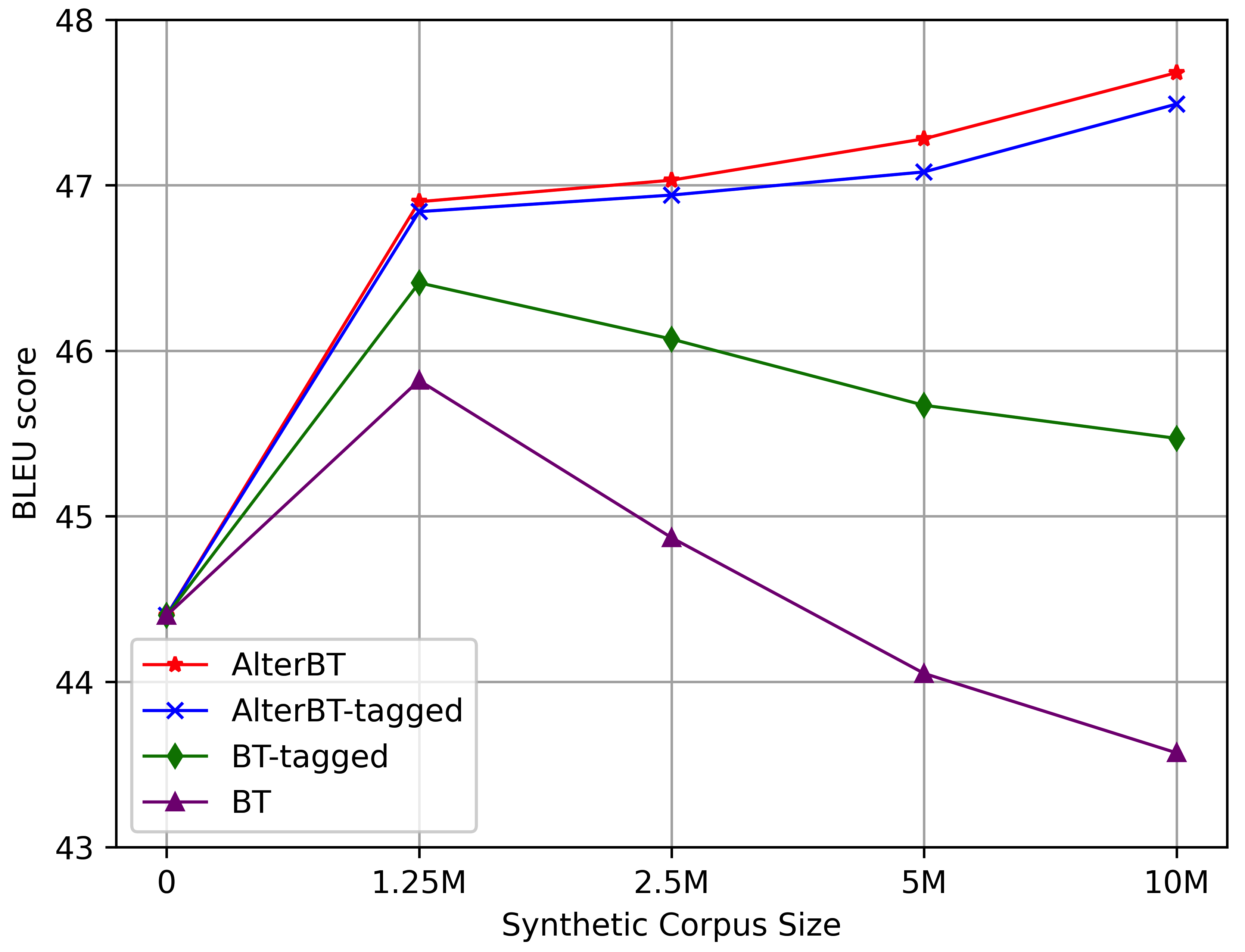
Figure 1: Comparison with several baselines in different data scale. Our alternated approach outperforms the conventional back-translation method and improves the performance of Tagged BT. Moreover, with the enlargement of the synthetic data scale, the BLEU score rises steadily by alternated training.

3.3 BLEU Landscape Visualization

To validate the assumption that the authentic data helps to rectify the deviation in synthetic data and redirect the NMT model parameters to a better optimization path, we further investigate the BLEU landscape to compare our method with the BT approach during the same training steps.

Figure 2: Visualization of BLEU landscape on NIST06 dataset defined by $\hat{\bm{\theta}}_{s}^{(t)}$, $\hat{\bm{\theta}}_{a}^{(t)}$ and $\hat{\bm{\theta}}_{s}^{(t+1)}$. The projected checkpoints are represented as stars. Starting from $\hat{\bm{\theta}}_{s}^{(t)}$, the red dashed and solid segments represent S-Step and A-Step in our method, respectively. The blue dashed segments illustrate the conventional BT method, which shares the same starting point $\hat{\bm{\theta}}_{s}^{(t)}$ with ours. $\hat{\bm{\theta}}_{\mathrm{BT}}^{(t+1)}$ denotes the BT model trained the same steps as $\hat{\bm{\theta}}_{a}^{(t+1)}$. It is shown that alternated training guides the model from $\hat{\bm{\theta}}_{s}^{(t)}$ to $\hat{\bm{\theta}}_{a}^{(t)}$, $\hat{\bm{\theta}}_{s}^{(t+1)}$ and $\hat{\bm{\theta}}_{a}^{(t+1)}$ successively, which finally leads to a better point with a higher BLEU score.

The visualization of the BLEU landscape is shown in Figure 2. Checkpoints during alternated training are projected onto the 2D plane defined by $\hat{\bm{\theta}}_{s}^{(t)}$, $\hat{\bm{\theta}}_{a}^{(t)}$ and $\hat{\bm{\theta}}_{s}^{(t+1)}$ . Our projection method considers both the model parameters and their translation performance (See Appendix A for details). For the conventional BT approach, the model parameters are stuck in an inefficient optimization path (highlighted in blue dashed lines). In our approach, we find that authentic data effectively guides the model towards a better direction for A-Step (highlighted in red solid lines). For S-Step (highlighted in red dashed lines), although training with synthetic data deteriorates the BLEU performance, it pushes the model away from the original route, and enables authentic data to further redirect the model into a better point with a higher BLEU score.

4 Related Work

Our work is based on back-translation (BT), an approach to leverage monolingual data by an additional target-to-source system. BT was proved to be effective in neural machine translation (NMT) systems (Sennrich et al., 2016a). Despite its effectiveness, BT is limited by the accuracy of synthetic data. Noise and translation errors hinder the boosting of model performance (Hoang et al., 2018). The negative results become more evident when more synthetic data is mixed into training data (Caswell et al., 2019; Wu et al., 2019).

Considerable studies have focused on the accuracy problem in synthetic data and further extended back-translation. Imamura et al. (2018) demonstrate that generating source sentences via sampling increases the diversity of synthetic data and benefits the BT system. Edunov et al. (2018) further propose a noisy beam search method to generate more diversified source-side data. Caswell et al. (2019) add a reserved token to synthetic source-side sentences in order to help NMT model distinguish between authentic and synthetic data. Another perspective aims at measuring the translation quality of synthetic data. Imamura et al. (2018) filter sentence pairs with low likelihood or low confidence. Wang et al. (2019) use uncertainty-based confidence to measure words and sentences in synthetic data. Different from the aforementioned works, our approach introduces neither data modification (e.g. noising or tagging) nor additional models for evaluation. We alternate training set on the original authentic and synthetic data.

The work relatively close to ours is Iterative Back-Translation (Hoang et al., 2018), which refines forward and backward model via back-translation data, and regenerates more accurate synthetic data from monolingual data. Our work differs from Iterative BT in that we do not require source-side monolingual corpora or repeatedly finetune the backward model.

5 Conclusion

In this work, we propose alternated training with synthetic and authentic data for neural machine translation. Experiments have shown the supremacy of our approach. Visualization of the BLEU landscape indicates that alternated training guides the NMT model towards better points.

Appendix A Method for Visualization

We first define the projection plane $S$ by parameters $\hat{\bm{\theta}}_{s}^{(t)}$, $\hat{\bm{\theta}}_{a}^{(t)}$ and $\hat{\bm{\theta}}_{s}^{(t+1)}$. Selecting $\hat{\bm{\theta}}^{*}=\hat{\bm{\theta}}_{s}^{(t)}$ as the basic point and $\boldsymbol{\delta}=\hat{\bm{\theta}}_{a}^{(t)}-\hat{\bm{\theta}}_{s}^{(t)},\boldsymbol{\eta}=\hat{\bm{\theta}}_{s}^{(t+1)}-\hat{\bm{\theta}}_{s}^{(t)}$ as two basis vectors, we plot the function $f(x,y)=\mathrm{BLEU}(D_{\mathrm{DEV}};\hat{\bm{\theta}}^{*}+x\boldsymbol{\delta}+y\boldsymbol{\eta})$ in the 2D surface. We calculate the BLEU scores for all NMT models defined by grid points on the projection plane, and construct the BLEU contours via linear interpolation in Matplotlib (Hunter, 2007).

We project the model checkpoints onto the 2D plane $S$ to represent the parameter geometry and their translation performance. As the 2D contour plane consists of several regions corresponded with different BLEU ranges, we formulate the visualization task into the following problem:

$$(x_{i},y_{i})=\mathop{\rm argmin}_{(x,y)\in S_{i}}{\left\|\hat{\bm{\theta}}_{i}-\left(\hat{\bm{\theta}}^{*}+x\boldsymbol{\delta}+y\boldsymbol{\eta}\right)\right\|_{F}^{2}},$$ (7)

where $S_{i}$ denotes the BLEU region that the performance of $\hat{\bm{\theta}}_{i}$ lies in. It is noted that according to the Pythagorean theorem, for $\forall~{}(\tilde{x},\tilde{y})\in S_{i}$,

$$\left\|\hat{\bm{\theta}}_{i}-\left(\hat{\bm{\theta}}^{*}+\tilde{x}\boldsymbol{\delta}+\tilde{y}\boldsymbol{\eta}\right)\right\|_{F}^{2}$$ (8)

$$= \left\|\hat{\bm{\theta}}_{i}-\left(\hat{\bm{\theta}}^{*}+\hat{x}_{i}\boldsymbol{\delta}+\hat{y}_{i}\boldsymbol{\eta}\right)\right\|_{F}^{2}+$$

$$\left\|\left(\hat{\bm{\theta}}^{*}+\hat{x}_{i}\boldsymbol{\delta}+\hat{y}_{i}\boldsymbol{\eta}\right)-\left(\hat{\bm{\theta}}^{*}+\tilde{x}\boldsymbol{\delta}+\tilde{y}\boldsymbol{\eta}\right)\right\|_{F}^{2},$$

where

$$(\hat{x}_{i},\hat{y}_{i})=\mathop{\rm argmin}_{(x,y)\in S}{\left\|\hat{\bm{\theta}}_{i}-\left(\hat{\bm{\theta}}^{*}+x\boldsymbol{\delta}+y\boldsymbol{\eta}\right)\right\|_{F}^{2}}.$$ (9)

As $(x_{i},y_{i})\in S_{i}$, we can substitute $(\tilde{x},\tilde{y})$ in Eq. (8) with $(x_{i},y_{i})$. Notice that the first term on the right-hand side of Eq. (8) is independent of $(x_{i},y_{i})$, the minimizer $(x_{i},y_{i})$ thus satisfies the following conditions:

$$(x_{i},y_{i})=\mathop{\rm argmin}_{(\tilde{x},\tilde{y})\in S_{i}}\Bigg{\|} \left(\hat{\bm{\theta}}^{*}+\hat{x}_{i}\boldsymbol{\delta}+\hat{y}_{i}\boldsymbol{\eta}\right)$$ (10)

$$-\left(\hat{\bm{\theta}}^{*}+\tilde{x}\boldsymbol{\delta}+\tilde{y}\boldsymbol{\eta}\right)\Bigg{\|}_{F}^{2},$$

with $(\hat{x}_{i},\hat{y}_{i})$ satisfying Eq. (9).

According to Eq. (8), our projection method can be divided into two steps. The first step is to calculate $(\hat{x}_{i},\hat{y}_{i})$ in Eq. (9), which minimizes the first term of Eq. (8). By the least square method, we obtain the analytic solution to $(\hat{x}_{i},\hat{y}_{i})$ as follows:

$$\begin{cases}x_{i}&=\frac{VB-UC}{B^{2}-AC},\\ y_{i}&=\frac{UB-VA}{B^{2}-AC},\end{cases}$$ (11)

where

$$A =\langle\boldsymbol{\delta},\boldsymbol{\delta}\rangle,$$ (12)

$$B =\langle\boldsymbol{\delta},\boldsymbol{\eta}\rangle,$$

$$C =\langle\boldsymbol{\eta},\boldsymbol{\eta}\rangle,$$

$$U =\langle\hat{\bm{\theta}}_{i}-\hat{\bm{\theta}}^{*},\boldsymbol{\delta}\rangle,$$

$$V =\langle\hat{\bm{\theta}}_{i}-\hat{\bm{\theta}}^{*},\boldsymbol{\eta}\rangle.$$

The second step is to solve $(x_{i},y_{i})$ in Eq. (10), which minimizes the second term of Eq. (8). Specially, we have $(x_{i},y_{i})=(\hat{x}_{i},\hat{y}_{i})$ if $(\hat{x}_{i},\hat{y}_{i})\in S_{i}$. Otherwise, as the BLEU region $S_{i}$ is enclosed by polygon boundaries with limited edges, we simply calculate the distance between $(\hat{x}_{i},\hat{y}_{i})$ and each edge and select the minimum one. The boundary point minimizing the distance is then determined as $(x_{i},y_{i})$. We cast the projection point from $(\hat{x}_{i},\hat{y}_{i})$ to $(x_{i},y_{i})$ in order to restore the origin BLEU performance of $\hat{\bm{\theta}}_{i}$.

References

- Bahdanau et al. (2015) Dzmitry Bahdanau, Kyunghyun Cho, and Yoshua Bengio. 2015. Neural machine translation by jointly learning to align and translate. In 3rd International Conference on Learning Representations, ICLR 2015.
- Caswell et al. (2019) Isaac Caswell, Ciprian Chelba, and David Grangier. 2019. Tagged back-translation. In Proceedings of the Fourth Conference on Machine Translation, WMT 2019, Florence, Italy, August 1-2, 2019 - Volume 1: Research Papers, pages 53–63. Association for Computational Linguistics.
- Cheng et al. (2016) Yong Cheng, Wei Xu, Zhongjun He, Wei He, Hua Wu, Maosong Sun, and Yang Liu. 2016. Semi-supervised learning for neural machine translation. In Proceedings of the 54th Annual Meeting of the Association for Computational Linguistics, ACL 2016, August 7-12, 2016, Berlin, Germany, Volume 1: Long Papers. The Association for Computer Linguistics.
- Edunov et al. (2018) Sergey Edunov, Myle Ott, Michael Auli, and David Grangier. 2018. Understanding back-translation at scale. In Proceedings of the 2018 Conference on Empirical Methods in Natural Language Processing, pages 489–500.
- Fadaee et al. (2017) Marzieh Fadaee, Arianna Bisazza, and Christof Monz. 2017. Data augmentation for low-resource neural machine translation. In Proceedings of the 55th Annual Meeting of the Association for Computational Linguistics (Volume 2: Short Papers), pages 567–573, Vancouver, Canada. Association for Computational Linguistics.
- Gehring et al. (2017) Jonas Gehring, Michael Auli, David Grangier, Denis Yarats, and Yann N Dauphin. 2017. Convolutional sequence to sequence learning. In International Conference on Machine Learning, pages 1243–1252.
- He et al. (2016) Di He, Yingce Xia, Tao Qin, Liwei Wang, Nenghai Yu, Tie-Yan Liu, and Wei-Ying Ma. 2016. Dual learning for machine translation. In Advances in Neural Information Processing Systems 29: Annual Conference on Neural Information Processing Systems 2016, December 5-10, 2016, Barcelona, Spain, pages 820–828.
- Hoang et al. (2018) Cong Duy Vu Hoang, Philipp Koehn, Gholamreza Haffari, and Trevor Cohn. 2018. Iterative back-translation for neural machine translation. In Proceedings of the 2nd Workshop on Neural Machine Translation and Generation, NMT@ACL 2018, Melbourne, Australia, July 20, 2018, pages 18–24. Association for Computational Linguistics.
- Hunter (2007) J. D. Hunter. 2007. Matplotlib: A 2d graphics environment. Computing in Science & Engineering, 9(3):90–95.
- Imamura et al. (2018) Kenji Imamura, Atsushi Fujita, and Eiichiro Sumita. 2018. Enhancement of encoder and attention using target monolingual corpora in neural machine translation. In Proceedings of the 2nd Workshop on Neural Machine Translation and Generation, NMT@ACL 2018, Melbourne, Australia, July 20, 2018, pages 55–63. Association for Computational Linguistics.
- Kingma and Ba (2015) Diederik P. Kingma and Jimmy Ba. 2015. Adam: A method for stochastic optimization. In Proceedings of ICLR.
- Koehn et al. (2007) Philipp Koehn, Hieu Hoang, Alexandra Birch, Chris Callison-Burch, Marcello Federico, Nicola Bertoldi, Brooke Cowan, Wade Shen, Christine Moran, Richard Zens, Chris Dyer, Ondrej Bojar, Alexandra Constantin, and Evan Herbst. 2007. Moses: Open source toolkit for statistical machine translation. In ACL 2007, Proceedings of the 45th Annual Meeting of the Association for Computational Linguistics, June 23-30, 2007, Prague, Czech Republic. The Association for Computational Linguistics.
- Sennrich et al. (2016a) Rico Sennrich, Barry Haddow, and Alexandra Birch. 2016a. Improving neural machine translation models with monolingual data. In Proceedings of the 54th Annual Meeting of the Association for Computational Linguistics, ACL 2016, August 7-12, 2016, Berlin, Germany, Volume 1: Long Papers. The Association for Computer Linguistics.
- Sennrich et al. (2016b) Rico Sennrich, Barry Haddow, and Alexandra Birch. 2016b. Neural machine translation of rare words with subword units. In Proceedings of the 54th Annual Meeting of the Association for Computational Linguistics, ACL 2016, August 7-12, 2016, Berlin, Germany, Volume 1: Long Papers. The Association for Computer Linguistics.
- Sun et al. (2016) Maosong Sun, Xinxiong Chen, Kaixu Zhang, Zhipeng Guo, and Zhiyuan Liu. 2016. Thulac: An efficient lexical analyzer for chinese.
- Sutskever et al. (2014) Ilya Sutskever, Oriol Vinyals, and Quoc V Le. 2014. Sequence to sequence learning with neural networks. In Advances in Neural Information Processing Systems, volume 27, pages 3104–3112. Curran Associates, Inc.
- Tan et al. (2020) Zhixing Tan, Jiacheng Zhang, Xuancheng Huang, Gang Chen, Shuo Wang, Maosong Sun, Huanbo Luan, and Yang Liu. 2020. THUMT: An open-source toolkit for neural machine translation. In Proceedings of the 14th Conference of the Association for Machine Translation in the Americas (Volume 1: Research Track), pages 116–122, Virtual. Association for Machine Translation in the Americas.
- Vaswani et al. (2017) Ashish Vaswani, Noam Shazeer, Niki Parmar, Jakob Uszkoreit, Llion Jones, Aidan N Gomez, Łukasz Kaiser, and Illia Polosukhin. 2017. Attention is all you need. In Advances in neural information processing systems, pages 5998–6008.
- Wang et al. (2019) Shuo Wang, Yang Liu, Chao Wang, Huanbo Luan, and Maosong Sun. 2019. Improving back-translation with uncertainty-based confidence estimation. In Proceedings of the 2019 Conference on Empirical Methods in Natural Language Processing and the 9th International Joint Conference on Natural Language Processing, EMNLP-IJCNLP 2019, Hong Kong, China, November 3-7, 2019, pages 791–802. Association for Computational Linguistics.
- Wu et al. (2019) Lijun Wu, Yiren Wang, Yingce Xia, QIN Tao, Jianhuang Lai, and Tie-Yan Liu. 2019. Exploiting monolingual data at scale for neural machine translation. In Proceedings of the 2019 Conference on Empirical Methods in Natural Language Processing and the 9th International Joint Conference on Natural Language Processing (EMNLP-IJCNLP), pages 4198–4207.
- Zhang and Zong (2016) Jiajun Zhang and Chengqing Zong. 2016. Exploiting source-side monolingual data in neural machine translation. In Proceedings of the 2016 Conference on Empirical Methods in Natural Language Processing, EMNLP 2016, Austin, Texas, USA, November 1-4, 2016, pages 1535–1545. The Association for Computational Linguistics.