Adiabatic topological pumping in a semiconductor nanowire

Abstract

The adiabatic topological pumping is proposed by periodically modulating a semiconductor nanowire double-quantum-dot chain. We demonstrate that the quantized charge transport can be achieved by a nontrivial modulation of the quantum-dot well and barrier potentials. When the quantum-dot well potential is replaced by a time-dependent staggered magnetic field, the topological spin pumping can be realized by periodically modulating the barrier potentials and magnetic field. We also demonstrate that in the presence of Rashba spin-orbit interaction, the double-quantum-dot chain can be used to implement the topological spin pumping. However, the pumped spin in this case can have a quantization axis other than the applied magnetic field direction. Moreover, we show that all the adiabatic topological pumping are manifested by the presence of gapless edge states traversing the band gap as a function of time.

I Introduction

In recent years adiabatic topological pumping has attracted considerable attentions as it plays an important role in implementing quantized particle transports Meidan2010 ; Citro2016 and in exploring higher-dimensional topological effects Prodan2015 ; Kraus2016 ; Zilberberg2018 ; Lohse2018 . The concept of topological pumping was first introduced by Thouless who showed that the quantization of charge transport can be realized by a cyclic modulation of a one-dimensional periodic potential adiabatically and the charge pumped per cycle can be determined by the Chern number defined over the two-dimensional Brillouin zone formed in the momentum and time spaces Thouless1983 ; Niu1984 . It has been confirmed that some low-dimensional systems, such as quasicrystals and optical supperlattices, can exhibit the higher-dimensional topological effects, when subjected to a nontrivial modulation, and can thus be used to implement the adiabatic topological pumping   Tangpanitanon2017 ; Ke2020 ; Lin2020 ; Kraus2012 ; Kraus2013 ; Verbin2015 ; Schweizer2016 ; Nakajima206 ; Lohse2015 . Recently, the Thouless pumping of ultracold bosonic/fermionic atoms in an optical superlattice has been experimentally achieved via periodically modulating the superlattice phase Nakajima206 ; Lohse2015 . However, up to now, realizations of the topological pumping are almost limited to the optical systems and, therefore, it is of interest to explore the exotic phenomena of topological pumping in low-dimensional systems made from conventional semiconductors.

Both experimentally and theoretically, the adiabatic quantum pumping of electron charge and spin in semiconductor nanostructures has been one of the hotspot issues Thomas1994 ; Brouwer1998 ; OEA2002 ; Altshuler1999 ; Switkes1999 ; Aleiner1998 ; Hasegawa2019 ; OEA2002a ; Aharony2002 ; Zhou1999 . Especially, the parametric pumping facilitates the adiabatic transfer of noninteracting electrons in unbiased quantum dots Brouwer1998 ; Switkes1999 ; OEA2002 , but the average transferred charge in a cycle is not necessarily quantized under such a parametric pumping scheme. It has been shown that the pumped number is quantized through the adiabatic topological pumping and the physics behind this deeply roots into the nontrivial topology of the periodic wave functions Xiao2010 ; Wang2013 ; Hatsugai2016 . Moreover, the presence of fractional boundary charges in quantum dot arrays has been theoretically demonstrated by manipulating the onsite potentials periodically Park2016 ; Thakurathi2018 . However, a systematic analysis of the topological pumping in a one-dimensional periodic semiconductor nanostructure is still scarce.

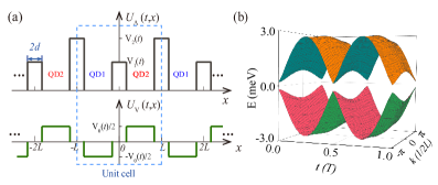
Figure 1: (color online) (a) Schematic diagrams of two periodic potentials $U_{\Lambda}(t,x)$ and $U_{V}(t,x)$ assumed in the implementation of the topological charge pumping in a semiconductor nanowire DQD chain. Specifically, $U_{\Lambda}(t,x)$ consists of barrier potentials $V_{1}(t)$ and $V_{2}(t)$ in a unit cell, with $2d$ denoting the width of each barrier potential and $2L$ being the unit-cell length, and $U_{V}(t,x)$ comprises two QD well potentials $\pm V_{0}(t)/2$. (b) 3D plot of the energy spectrum for the two lowest-energy Bloch bands of the periodic DQD chain with the parameter vector $\widehat{V}=(V_{0},\delta V)$ driven by a nontrivial modulation. Here the parameters used in the calculations are $m^{\ast}=0.023m_{0}$ ($m_{0}$ is the free electron mass), $2L=120$ nm, $2d=20$ nm, $\varepsilon_{0}=6.0$ meV, and the sum of the two barrier potentials $V_{2}(t)+V_{1}(t)=36$ meV.

In this paper, we propose a scheme for implementing the adiabatic topological pumping in a semiconductor nanowire double-quantum-dot (DQD) chain. We first demonstrate that the topological charge pumping can be achieved by simultaneously modulating the quantum-dot well and barrier potentials of the DQD chain. In the absence of the quantum-dot well potential modulation, we show that the topological spin pumping can be achieved by employing a time-dependent staggered magnetic field and by a nontrivial modulation of the barrier potentials and magnetic field in a cycle. When the DQD chain of a finite length is coupled to the external leads, we show that the quantized charge and spin transport can be calculated by exploiting the scattering matrix formalism under a nontrivial modulation. Especially, we demonstrate the quantized spin pumping in the presence of the Rashba spin-orbit interaction (SOI), but the pumped spin can have the spin quantization axis different from the applied staggered magnetic field direction. We also demonstrate, based on the changing of time-reversal charge polarization in a half cycle, that the periodic DQD chain in the presence of SOI can serve as a dynamic version of a topological insulator under a nontrivial modulation of the barrier potentials and magnetic field.

The rest part of the paper is organized as follows. In Sec. II, a periodic potential to define the DQD chain in a one-diemnsional semiconductor is introduced and the implementation of topological charge pumping is demonstrated. In Sec. III, the topological spin pumping in the semiconductor DQD chain in the presence of a time-dependent staggered magnetic field is analyzed. Section IV devotes to the formalism for calculating the charge and spin pumping through a finite DQD chain under topological modulations. In the presence of the Rashba SOI, the topological spin pumping in the periodic DQD chain is discussed in Sec. V. Finally, we summarize the paper in Sec. VI.

II Topological charge pumping

We first consider a periodic semiconductor nanowire DQD system subjected to time-dependent periodic barrier potential $U_{\Lambda}(t,x)$ and quantum-dot well potential $U_{V}(t,x)$, as shown in Fig. 1(a), described by the effective one-dimensional Hamiltonian,

$$H_{0}=\frac{p^{2}}{2m^{\ast}}+U_{\Lambda}(t,x)+U_{V}(t,x)\ ,$$ (1)

where $p=-i\hbar\frac{\partial}{\partial x}$ represents the momentum operator and $m^{\ast}$ is the effective electron mass. In this system, a unit cell, as indicated by the dashed square in Fig. 1(a), comprises two quantum dots (QDs), labeled as QD1 and QD2. Structurally, $U_{\rm\Lambda}(t,x)$ consists of barrier potentials $V_{1}(t)$ and $V_{2}(t)$ and $U_{\rm V}(t,x)$ comprises two QD well potentials $\pm V_{0}(t)/2$ in a unit cell. Explicitly, for a unit cell of $-L\leq x<L$, the two potentials can be written as

$$U_{\rm V}(t,x)= \frac{1}{2}V_{0}(t)[f^{+}_{1}(x)-f^{+}_{2}(x)],$$

$$U_{\rm\Lambda}(t,x)= V_{1}(t)f^{-}_{1}(x)+V_{2}(t)[1+f^{-}_{2}(x)]\ ,$$ (2)

where $2L$ denotes the size of unit cell, $2d$ ($2d\ll 2L$) the width of each potential barrier, $f^{\pm}_{1}(x)=\Theta(x+d)\pm\Theta(x-d)$ and $f^{\pm}_{2}(x)=\Theta(x+d-L)\pm\Theta(x+L-d)$, with $\Theta(x)$ being the Heaviside function, the spatial distribution functions.

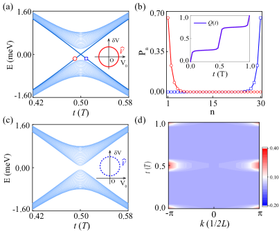
Figure 2: (color online) (a) Energy spectrum of a finite DQD chain comprising 30 unit cells versus $t$ under a nontrivial modulation of $\widehat{V}=(V_{0},\delta V)$ with $\varepsilon_{0}=6.0$ meV and a changing contour of $\widehat{V}$ as displayed in the inset. (b) Probability density distributions, $P_{n}$, calculated for the two gapless band states of the finite DQD chain, as indicated by the circle and square symbols in (a). Inset shows the calculated time-evolution of charge polarization $\mathcal{Q}(t)$. (c) The same as (a), but under a trivial modulation with $\varepsilon_{0}=6.0$ meV and $\varepsilon_{\iota}=8.0$ meV. (d) Berry curvature $F(k,t)$ calculated as a function of $k$ and $t$ for the occupied Bloch band of the corresponding infinite DQD chain under the nontrivial modulation as shown in the inset of (a). All other parameters employed are the same as in Fig. 1.

In fact, the topological charge pumping can be achieved by a nontrivial modulation of system parameters $V_{0}(t)$ and $\delta V(t)\equiv V_{2}(t)-V_{1}(t)$. To see this, we consider the case that there is only one energy level in each QD and rewrite Hamiltonian Eq. (1) in the second quantization form

$$H_{\rm 0,T}= \sum_{n}\left(t_{\rm in,0}a^{\dagger}_{n}b_{n}+t_{\rm ex,0}a^{\dagger}_{n+1}b_{n}+\rm{h.c.}\right)$$

$$~{}~{}-\frac{\Delta_{0}}{2}\sum_{n}\left(a^{\dagger}_{n}a_{n}-b^{\dagger}_{n}b_{n}\right)\ ,$$ (3)

with $n$ representing the unit-cell index, $a^{\dagger}_{n}$ ($a_{n}$) and $b^{\dagger}_{n}$ ($b_{n}$) denoting the creation (annihilation) operators of the energy levels in QD1 and QD2 of the $n$th unit cell, $t_{\rm in/ex,0}$ being the intra/inter unit-cell hopping amplitudes, and $\pm\Delta_{0}/2$ the effective on-site energies (i.e., the level energies) in QD1 and QD2. Note that the Hamiltonian in Eq. (3) is derived from Eq. (1) by subtracting a constant potential value and this Hamiltonian is identical to the Rice-Mele model Hamiltonian Rice1982 . In analogy with the Thouless pumping in Refs. Nakajima206, ; Lohse2015, , it is found that the topological charge pumping can be realized when the changing trajectory of the parameter vector $(\Delta_{0},\delta t_{0})$, with $\delta t_{0}=t_{\rm in,0}-t_{\rm ex,0}$, obeys a nonzero winding number in a period. Here, because $\Delta_{0}$ and $\delta t_{0}$ can be regulated by potentials $V_{0}$ and $\delta V$, respectively, we can deduce that the topological charge pumping can be implemented if the changing contour of the modulation vector $\widehat{V}=(V_{0},\delta V)$ possesses a nonzero winding number in a cycle.

For an infinite periodic DQD chain system under a nontrivial modulation with $V_{0}(t)=\varepsilon_{0}\sin(2\pi t/T)$ and $\delta V(t)=\varepsilon_{0}\cos(2\pi t/T)$, a three-dimensional (3D) plot of the energy spectrum for the two lowest-energy Bloch bands is displayed in Fig. 1(b), where $\varepsilon_{0}$ is the energy modulation amplitude, $T$ is the cyclic time of the pumping and $k$ is the wave vector in a unit of $1/(2L)$. It is seen in Fig. 1(b) that the energies of the two lowest-energy Bloch bands vary with time and are separated by a nonzero bandgap throughout the pumping. Figure 2(a) shows the energy spectrum of a finite DQD chain under the same modulation of $V_{0}(t)=\varepsilon_{0}\sin(2\pi t/T)$ and $\delta V(t)=\varepsilon_{0}\cos(2\pi t/T)$. Here it is seen that two gapless bands are present in the Bloch band gap. Figure 2(b) shows the probability density distributions of two gapless band states at a selected energy. Here, it is seen that the two gapless band states are highly localized at the ends of the DQD chain. Thus these gapless band states are of edge states as one commonly observes in a topological insulator. Figure 2(c) shows the energy spectrum of the finite DQD chain under a trivial modulation of $V_{0}(t)=\varepsilon_{0}\sin(2\pi t/T)$, $\delta V(t)=\varepsilon_{\iota}+\varepsilon_{0}\cos(2\pi t/T)$ with the shifting energy $\varepsilon_{\iota}>\varepsilon_{0}$. It is evident that no gapless edge state is presented in this trivial modulation case. Here and hereafter, we assume that the periodic DQD chain is defined in an InAs nanowire with $m^{\ast}=0.023m_{0}$ Winkler2003 ($m_{0}$ is the free electron mass), $2L=120$ nm, $2d=20$ nm, $\varepsilon_{0}=6.0$ meV, and the sum of the two barrier potentials fixed as $V_{2}(t)+V_{1}(t)=36$ meV, and the cyclic time $T$ is large enough to ensure the adiabaticity of pumping.

Based on the bulk-boundary correspondence Hatsugai2016 , the presence of the gapless edge states is correlated to the nontrivial topology of the chain with periodic boundary conditions. By regarding the time as a virtual momentum axis orthogonal to the wire axis, the Berry curvature of a Bloch band in the two-dimensional Brillouin zone can be introduced Thouless1983 ; Wang2013 ,

$$F(k,t)=i\left(\langle\partial_{k}u|\partial_{t}u\rangle-\langle\partial_{t}u|\partial_{k}u\rangle\right)\ ,$$ (4)

with $|u(k,t)\rangle$ being the Bloch function below the energy gap, and the nontrivial topology is quantified by a nonzero Chern number Thouless1983 ; Wang2013 ,

$$\mathcal{C}=\frac{1}{2\pi}\int^{T}_{0}\int^{\pi}_{-\pi}F(k,t)dtdk\ .$$ (5)

For the case of a nontrivial modulation as illustrated in the inset of Fig. 2(a), the calculated distribution of the Berry curvature on the $k-t$ plane is displayed in Fig. 2(d). Numerical evaluation of Eq. (5) performed as in Ref. Fukui2005, verifies the nonzero Chern number of $\mathcal{C}=1$, confirming that the DQD chain under the nontrivial modulation is in the topological nontrivial phase. In addition, based on the theory of topological polarization Smith1993 ; Asboth2016 , $\mathcal{Q}(t)=\frac{1}{2\pi}\int^{t}_{0}\int^{\pi}_{-\pi}F(k,t)dtdk$ can be interpreted as the time-dependent charge polarization (in a unit of $-e$) and the topological charge pumping can be visualized by the time-evolution of $\mathcal{Q}(t)$ in a cycle, just as shown in the inset of Fig. 2(b), with $\mathcal{Q}(T)=1$ under this nontrivial modulation.

III Topological spin pumping

Figure 3: (color online) (a) Schematic diagram of the DQD chain in the absence of QD well potential modulation but with the electron spin modulated by a time-dependent staggered magnetic field $B(t,x)$ applied in the $z$ direction. (b) Schematic for the staggered external magnetic field $B(t,x)$.

In this section, the implementation of topological spin pumping is proposed in the periodic DQD chain with a time-dependent staggered magnetic field $B(t,x)$ applied in a direction perpendicular to the wire axis, say the $z$ direction, as shown in Fig. 3(a). Here, we set the QD well potential unmodulated but keep modulation on the barrier potential difference $\delta V(t)$. The Hamiltonian of the periodic DQD chain system can now be written as

$$H_{\rm Z}=\frac{p^{2}}{2m^{\ast}}+U_{\rm\Lambda}(t,x)+\frac{g^{\ast}\mu_{\rm B}B(t,x)}{2}\sigma_{z}\ ,$$ (6)

with $g^{\ast}$ being the electron Landé factor, $\mu_{\rm B}$ the Bohr magneton, and $\boldsymbol{\sigma}=(\sigma_{x},\sigma_{y},\sigma_{z})$ representing the three Pauli matrices. Specifically, the time-dependent staggered magnetic field [see Fig. 3(b)] within a unit cell of $-L\leq x<L$ takes the form of

$$B(t,x)=B(t)\left[f^{+}_{1}(x)-f^{+}_{2}(x)\right]\ ,$$ (7)

with $B(t)$ denoting the strength of the field and $f^{+}_{1}(x)$ and $f^{+}_{2}(x)$ representing the same spatial functions as before. It is important to note that the effect of the vector potential within the Landau gauge, i.e, $\mathbf{A}=(-By,0,0)$, is ignored in Eq. (6), due to the one-dimensional nature of the system, i.e., an extremely strong confinement in the transverse directions of the nanowire.

Using the commutation relation $[H_{\rm Z},\sigma_{z}]=0$, the Hamiltonian of the periodic DQD chain in the second quantization form can be written as

$$H_{\rm Z,T}=H_{\rm Z,\uparrow}+H_{\rm Z,\downarrow}\ ,$$ (8)

with the two spin-polarized terms given by

$$H_{\rm Z,\chi=\uparrow/\downarrow}= \sum_{n}\left(t_{{\rm in},0}a^{\dagger}_{n,\chi}b_{n,\chi}+t_{{\rm ex},0}a^{\dagger}_{n+1,\chi}b_{n,\chi}+{\rm{h.c.}}\right)$$

$$~{}~{}~{}\mp\frac{\Delta_{\rm z}}{2}\sum_{n}\left(a^{\dagger}_{n,\chi}a_{n,\chi}-b^{\dagger}_{n,\chi}b_{n,\chi}\right).$$ (9)

Here, the subscripts $\chi=\uparrow,\downarrow$ are spin indexes with the two spin states satisfying $\sigma_{z}|\uparrow\rangle=|\uparrow\rangle$ and $\sigma_{z}|\downarrow\rangle=-|\downarrow\rangle$, $a^{\dagger}_{n,\chi}$ ($a_{n,\chi}$) and $b^{\dagger}_{n,\chi}$ ($b_{n,\chi}$) are the creation (annihilation) operators of the electron spin states locating in the two QDs in the $n$th cell, and $\Delta_{\rm z}(t)=g^{\ast}\mu_{\rm B}B(t)$ is the time-dependent Zeeman splitting energy.

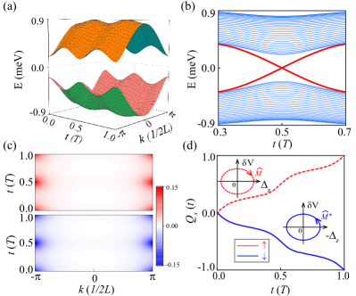
Figure 4: (color online) (a) 3D plot of the energy spectrum of the Bloch bands for the periodic DQD chain with the parameter vector $\widehat{M}=(\Delta_{\rm z},\delta V)$ driven by a nontrivial modulation as shown in the inset of (d) with $\varepsilon_{z}=0.9$ meV and $\varepsilon_{0}=6.0$ meV. (b) Energy spectrum of a correponding finite DQD chain of 30 unit cells versus $t$ under the nontrivial modulation. (c) Two spin-dependent Berry curvatures $F_{\chi=\uparrow,\downarrow}(k,t)$ calculated for the infinite DQD chain as a function of $k$ and $t$. The upper and lower panels show the results for the spin-up and spin-down Bloch bands. (d) The time-evolutions of the pumped spin polarizations $\mathcal{Q}_{\chi=\uparrow,\downarrow}(t)$ under this nontrivial modulation. The changing trajectories of the two parameter vectors $\widehat{M}=(\Delta_{\rm z},\delta V)$ and $\widehat{M}^{\ast}=(-\Delta_{\rm z},\delta V)$ are shown in the inset with the arrows indicating the winding directions. The other parameters employed are the same as in Fig. 1.

To achieve topological spin pumping in this system, we consider a nontrivial modulation of the parameter vector $\widehat{M}=(\Delta_{\rm z},\delta V)$ in a cycle. For the spin-up term, by mapping $\Delta_{\rm z}$ to $\Delta_{0}$, the Hamiltonian $H_{\rm Z,\uparrow}$ in Eq. (9) is equivalent to the Hamiltonian $H_{0,T}$ in Eq. (3) and, therefore, the spin-up electron is pumped when the changing trajectory of $\widehat{M}$ has a nonzero winding number in a cycle. The analysis can also be applied to the spin-down electron with the parameter vector $\widehat{M}$ replaced by $\widehat{M}^{\ast}=(-\Delta_{\rm z},\delta V)$. Figure 4(a) shows a 3D plot of the energy spectrum for the Bloch bands of the DQD chain under a nontrivial modulation of $\Delta_{\rm z}(t)=\varepsilon_{z}\sin(2\pi t/T)$ and $\delta V(t)=\varepsilon_{0}\cos(2\pi t/T)$. Here, we see again that the energies of the two lowest-energy Bloch bands vary with time and are separated by a nonzero bandgap throughout the pumping. Note that, due to the spin degeneracy, each energy band shown in Fig. 4(a) is twofold degenerate and comprised of two different spin states. Figure 4(b) shows the corresponding energy spectrum of a finite DQD chain under this nontrivial modulation. It is evident that two gapless edge-state Bloch bands indicated by the thick red curves are prresent in the bulk band gap. Because the modulation vectors $\widehat{M}$ and $\widehat{M}^{\ast}$ have different winding directions in a cycle [see the inset of Fig. 4(d)], the spin-up and spin-down electrons are therefore propagated in the opposite directions and results in the effective quantized spin pumping.

To further illustrate this point, the Berry curvatures of the two spin-polarized Bloch bands are introduced $F_{\chi=\uparrow,\downarrow}(k,t)=i\big{(}\langle\partial_{k}u_{\chi}|\partial_{t}u_{\chi}\rangle-\langle\partial_{t}u_{\chi}|\partial_{k}u_{\chi}\rangle\big{)}$, with $|u_{\chi}(k,t)\rangle$ denoting the spin-dependent Bloch functions below the energy gap. Figure 4(c) shows the distributions of the two Berry curvatures on the $k-t$ plane under this nontrivial modulation. Figure 4(d) displays the corresponding time-evolution of the pumped spin polarization $\mathcal{Q}_{\chi}(t)=\frac{1}{2\pi}\int^{t}_{0}\int^{\pi}_{-\pi}F_{\chi}(k,t)dkdt$. The different signs in $\mathcal{Q}_{\uparrow}(t)$ and $\mathcal{Q}_{\downarrow}(t)$ implies the different propagating directions of the two spin polarizations Schweizer2016 and the topological spin pumping (in a unit of $-\hbar$) in a cycle becomes $\frac{1}{2}\big{[}\mathcal{Q}_{\uparrow}(T)-\mathcal{Q}_{\downarrow}(T)\big{]}=1$. In addition, the equality $\mathcal{Q}_{\uparrow}(T)+\mathcal{Q}_{\downarrow}(T)=0$ demonstrates no net charge pumping in the whole process.

IV Topological pumping in a finite DQD chain

In this section, we consider the case of a finite DQD chain coupled to two external leads, as illustrated in Fig. 5(a). The electron energy spectrum of the two semi-infinite leads in the momentum space can be derived as $E=2J_{0}\cos(k)$, with $J_{0}$ denoting the inter-site tunneling coupling strength in the leads and $J^{\prime}$ being the strength of the tunneling coupling of the leads to the finite DQD chain (comprising $N$ cells or $2N$ sites). The eigenstates of the leads are the degenerate plane waves $\exp\left(\pm ikl\right)$ Aharony2002 , with the site index $l\leq 0$ for the left lead and $l\geq 2N+1$ for the right lead. When the finite chain is subjected to an incoming wave from the left side, the scattered solutions of the two leads takes the form of OEA2002a

$$|\psi\rangle=\begin{cases}\exp(ikl)+\mathcal{R}(t)\exp(-ikl)~{}~{}~{}~{}~{}~{}l\leq 0\ ,\\ \mathcal{T}(t)\exp(ikl)~{}~{}~{}~{}~{}~{}~{}~{}~{}~{}~{}~{}~{}~{}~{}~{}~{}~{}l\geq 2N+1\ ,\end{cases}$$ (10)

with $\mathcal{T}(t)$ and $\mathcal{R}(t)$ representing the time-dependent transmission and reflection coefficients, respectively. Practically, the two time-dependent coefficients and the transferred charge or spin in a cycle can be ascertained by the second quantization Hamiltonian of the system based on the scattering matrix method Brouwer1998 ; Zhou1999 .

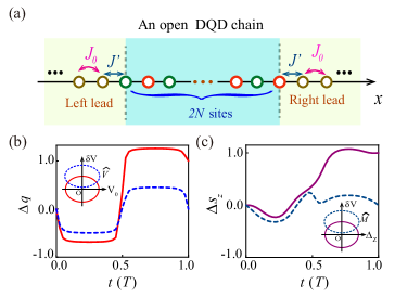
Figure 5: (color online) (a) Schematic diagram of a finite DQD chain (comprising $2N$ sites) coupled to two external leads with $J_{0}$ being the inter-site coupling strength in the leads and $J^{\prime}$ the strength of the tunneling coupling of the leads to the DQD chain. (b) Transferred charge $\Delta q$, in a unit of $-e$, as a function of $t$ with the parameter vector $\widehat{V}=(V_{0},\delta V)$ driven by a nontrivial and a trivial modulations as illustrated by the solid line and the dashed line in the inset of the panel. (c) Transferred spin $\Delta s_{z}$, in a unit of $-\hbar$, versus $t$ for the finite DQD chain with the parameter vector $\widehat{M}=(\Delta_{\rm z},\delta V)$ driven by a nontrivial and a trivial modulation as illustrated by the solid line and the dashed line in the inset of the panel. Here, parameters $\varepsilon_{z}=0.9$ meV, $\varepsilon_{0}=6.0$ meV, and $\varepsilon_{\iota}=8.0$ meV are employed in the calculations and the other ones are the same as in Fig. 1.

For a spinless chain, the second quantization Hamiltonian of the finite DQD chain is given by Eq. (3) and the reflection coefficient can be determined by the transfer matrix method (see Appendix). In terms of the reflection coefficient, the transferred charge in a cycle can be expressed as

$$\Delta q=\frac{e}{2\pi i}\int^{T}_{0}\frac{\mathcal{R}(t)}{dt}\mathcal{R}^{\ast}(t)dt\ .$$ (11)

For a spinful DQD chain, $\boldsymbol{\mathcal{R}}(t)$ corresponds to a $2\times 2$ matrix in spin space and the transferred spin per cycle can be derived as Meidan2010 ; Fu2006

$$\Delta\boldsymbol{\hat{s}}=\frac{\hbar}{2\pi i}\int^{T}_{0}{\mathrm{T}r}\left[\frac{\boldsymbol{\mathcal{R}}(t)}{dt}\boldsymbol{\hat{\sigma}}\boldsymbol{\mathcal{R}}^{\dagger}(t)\right]dt.$$ (12)

In the absence of spin-orbit interaction, $\boldsymbol{\mathcal{R}}(t)$ can be simplified to a diagonal form and the pumped spin is polarized by the external magnetic field along the $z$ direction. Below, we will demonstrate the quantized charge and spin transports in a short DQD chain under the nontrivial modulation described above.

Figure 5(b) shows the time evolutions of the transferred charge through a finite DQD chain with $N=9$, $J_{0}=0.4$ meV, $J^{\prime}=0.3$ meV, $k\simeq\pm\pi/2$, and under the two different modulations as illustrated in the inset of the figure. Here, the effective charge pumping, i.e., $\Delta q=1$, is observed when the parameter vector $\widehat{V}$ is subjected to a nontrivial modulation [see the red solid line]. The conclusion can also be applied to the spin pumping, but with the modulation vector $\widehat{V}$ replaced by $\widehat{M}=(\Delta_{\rm z},\delta V)$. Figure 5(c) shows the time evolutions of the transferred spin $\Delta s_{z}$ under two different modulations. It is also evident that the transferred spin becomes quantized under a nontrivial modulation (see the purple solid line) and is zero under a trivial modulation with $\Delta_{\rm z}(t)=\varepsilon_{z}\cos(2\pi t/T)$, $\delta V(t)=\varepsilon_{\iota}+\varepsilon_{0}\cos(2\pi t/T)$ and the shifting energy $\varepsilon_{\iota}>\varepsilon_{0}$ (see the blue dashed line).

V Topological spin pumping in the presence of spin-orbit interaction

It is well known that the spin-orbit interaction (SOI) plays an important role in the development of the topological insulator Hasan2010 ; Qi2011 ; Kane2005 ; Bernevig2006 . In this section, we will show that in the presence of the Rashba SOI, the DQD chain can serve as a dynamic version of a topological insulator and a spin pump if the parameter vector $\widehat{M}=(\Delta_{\rm z},\delta V)$ is driven by a nontrivial modulation.

The Hamiltonian of the DQD chain in the presence of the staggered magnetic field and the Rashba SOI can be written as

$$H=H_{\rm Z}+\alpha p\sigma_{y}\ ,$$ (13)

where $H_{\rm Z}$ is to the Hamiltonian given in Eq. (6) and $\alpha$ represents the strength of the SOI, which is related to the spin-orbit length $x_{\rm so}=\hbar/(m_{\rm e}\alpha)$. For $x_{\rm so}\gg L$, the Hamiltonian of the DQD chain in the second quantization form can be derived as

$$H_{\rm T}= \sum_{n}\left(a^{\dagger}_{n}t_{\rm in}b_{n}+a^{\dagger}_{n+1}t_{\rm ex}b_{n}+\rm{h.c.}\right)$$

$$-\frac{\Delta_{\rm z}}{2}\sum_{n}\left(a^{\dagger}_{n}\sigma_{z}a_{n}-b^{\dagger}_{n}\sigma_{z}b_{n}\right)\ ,$$ (14)

where $a_{n}=\{a_{n,\Uparrow},a_{n,\Downarrow}\}$ and $b_{n}=\{b_{n,\Uparrow},b_{n,\Downarrow}\}$ represent the spinors constituted of two spin-orbit states in the QDs and the intra/inter-cell tunneling amplitudes can be expressed as

$$t_{\rm in/ex}=t_{\rm in/ex,0}\exp[i\varphi_{\rm in/ex}\sigma_{x}]\ ,$$ (15)

with $\varphi_{\rm in/ex}$ being the functions of $L/x_{\rm so}$. In fact, the phase factors appearing in the right side of Eq. (15) arise purely from the interdot electron tunneling in the presence of the SOI AC1984 ; Shahbazyan1994 ; Liu2021 .

Figure 6: (color online) (a) 3D plot of the energy spectrum for the four lowest-energy Bloch bands of the same DQD chain as in Figs. 3 and 4, but in the presence of the Rashba SOI with a spin-orbit length of $x_{\rm so}=180$ nm, with the parameter vector $\widehat{M}=(\Delta_{z},\delta V)$ driven by a nontrivial modulation as shown by the solid line in the inset of (d) with $\varepsilon_{z}=0.9$ meV and $\varepsilon_{0}=6.0$ meV. (b) Energy spectrum of a corresponding finite chain consisting of $30$ unit cells as a function of $t$ under the same nontrivial modulation. Inset shows the time evolutions of the charges on the two Wannier centers, $\bar{x}_{\nu=1,2}$, in a unit cell of the infinite DQD chain. (c) The same as (b), but for the finite DQD chain under a trivial modulation with $\varepsilon_{z}=0.9$ meV, $\varepsilon_{0}=6.0$ meV and $\varepsilon_{\iota}=8.0$ meV. (d) Transferred spin components $|\Delta s_{z}|^{2}$ (higher value line) and $|\Delta s_{y}|^{2}$ (lower value line) calculated for the finite DQD chain against $t$. The solid and dashed lines are the results of the calculations for the finite DQD chain with the parameter vector $\widehat{M}$ driven by under the nontrivial (solid line) and trivial (dashed line) modulations as shown in the inset. All other undpecified parameters employed here are the same as in Fig. 1.

Figure 6(a) shows a 3D plot of the energy spectrum for the four lowest-energy Bloch bands of the DQD chain with $x_{\rm so}=180$ nm Scherubl2016 and with the parameter vector $\widehat{M}$ driven by the nontrivial modulation as illustrated by the solid line in the inset of Fig. 6(d). In contrast to the case without SOI, it indicates that the twofold degeneracy is generally lifted, except in the case of $t=0$, $T/2$, and $T$, for which the staggered magnetic field is zero and the system exhibits the Kramers’ degeneracy. Figure 6(b) shows the energy spectrum of a corresponding finite chain. As expected, there exist two pairs of gapless edge-state Bloch bands crossing the band gap in the finite system under this nontrivial modulation. Figure 6(c) shows the energy spectrum of the finite DQD chain under a trivial modulation as illustrated by the blue dashed line in the inset of Fig. 5(d). Clearly, there is no edge-state bands in the band gap in this case.

In analogy with a topological insulator, the presence of the gapless edge-state band in the band gap is correlated with the changing of time-reversal polarization in a half cycle Fu2006 . To be more specific, this kind of polarization is determined by the difference between the charges on the two Wannier centers in a unit cell constructed from the Bloch functions of the occupied bands Soluyanov2011 ; Yu2011 ,

$$\mathcal{P}(t)=\bar{x}_{1}(t)-\bar{x}_{2}(t)\ ,$$ (16)

where $\bar{x}_{1}(t)$ and $\bar{x}_{2}(t)$ represent the time-dependent charges on the Wannier centers in a unit cell with $x_{\nu=1,2}(t)\in[-0.5,0.5]$. The changing of time-reversal polarization in a half cycle can actually be identified as the (double-valued) $\mathbb{Z}_{2}$ invariant and the gapless edge states only appear when the topological invariant is nonzero Fu2006 . The inset of Fig. 6(b) shows the time-evolutions of the charges on the two Wannier centers in a unit cell of the infinite DQD chain under the nontrivial modulation. Indeed, it shows that the time-reversal polarization is increased by one in a half cycle, i.e., $\mathcal{P}(T/2)-\mathcal{P}(0)=1$, and this is in contrast to a trivial modulation for which $\mathcal{P}(T/2)-\mathcal{P}(0)=0$, see the inset of Fig. 6(c). Therefore, the periodic DQD chain can serve as a dynamical version of a topological insulator, with the topological property determined by the changing trajectory of $\widehat{M}$.

Similar to the topological spin pumping stated in Sec. III, there is no net charge pumped in a fully cycle and, because of the spin-orbit interaction, the spin pumped per cycle is no longer with the quantization axis along the $z$ direction. However, the results of the spin pumping depends on whether the changing of the parameter vector $\widehat{M}$ is in a trivial or nontrivial trajectory in a cycle. Figure 6(d) shows the time evolutions of the transferred spin in a finite DQD chain with the spin-orbit length $x_{\rm so}=180$ nm and the vector $\widehat{M}$ driven by the two different modulations as illustrated in the inset of the figure. It is evident that the spin transferred per cycle is nonzero under the nontrivial modulation (see the solid lines). Here, we would like to note that for this particular case the pumped spin has both $z$ and $y$ components. It is also clearly seen that the spin transferred in a cycle is zero under a trivial modulation (see the dashed curves).

VI Conclusion

In this paper, we propose a scheme to implement adiabatic topological pumping in a semiconductor nanowire DQD chain. The topological property of the pumping is related to the changing trajectory of the modulation parameters. We show that the topological charge pumping can be achieved by periodically modulating the QD well and barrier potentials, simultaneously, and the quantized charge transfer can only be realized if the corresponding changing contour is characterized with a nonzero winding number in a cycle. When the QD well potential is replaced by a time-dependent staggered magnetic field, the topological spin pumping can be achieved by a nontrivial modulation of the barrier potentials and magnetic field. We, in addition, demonstrate that in the presence of the Rashba SOI, the periodic DQD chain can serve as a dynamic version of a topological insulator and as a spin pump under a nontrivial modulation of the barrier potentials and magnetic field. Even though the topological adiabatic pumping studied in this paper is based on an InAs nanowire, it can also be extended to other 1D nanostructures, such as carbon nanotubes and Ge/Si heterostructure nanowires Biercuk2005 ; Hu2007 , with long spin-relaxation times. Our theoretical study presented in this work should boost the exploration of adiabatic topological pumping and higher-dimensional topological phases of matter in one-dimensional semiconductor nanostructures.

ACKNOWLEDGMENTS

This work is supported by the Ministry of Science and Technology of China through the National Key Research and Development Program of China (Grant Nos. 2017YFA0303304 and 2016YFA0300601), the National Natural Science Foundation of China (Grant Nos. 91221202, 91421303, and 11874071), the Beijing Academy of Quantum Information Sciences (No. Y18G22), and the Key-Area Research and Development Program of Guangdong Province (Grant No. 2020B0303060001).

CONFLICT OF INTEREST

The authors have no conflicts to disclose.

DATA AVAILABILITY

The data that support the findings of this study are available from the corresponding author upon reasonable request.

Appendix: DERIVATION OF THE REFLECTION COEFFICIENT

In this appendix, the detailed derivation for the reflection coefficient $\mathcal{R}(t)$ of a finite DQD chain coupled to two external leads is given.

Based on the discrete model shown in Fig. 5(a), the Hamiltonian of the total system can be written in the second quantization form as

$$H_{\rm tot}=H_{\rm DQD}+H_{\rm L}+H_{\rm R}+H_{\rm C}\ ,$$ (A1)

where $H_{\rm DQD}$ is the Hamiltonian of the finite DQD chain, $H_{\rm L/R}$ the Hamiltonian of the lead locating in the left/right side of the chain, and $H_{\rm C}$ describes the coupling between the leads and the DQD chain. For a finite DQD chain comprised by $N$ DQD cells, the Hamiltonian can be explicitly written as

$$H_{\rm DQD}= \sum^{N}_{n=1}\left(t_{\rm in,0}a^{\dagger}_{n}b_{n}+t_{\rm ex,0}\xi_{n}a^{\dagger}_{n+1}b_{n}+\rm{h.c.}\right)-\frac{\Delta_{0}}{2}$$

$$\times\sum^{N}_{n=1}\left(a^{\dagger}_{n}a_{n}-b^{\dagger}_{n}b_{n}\right)\ ,$$ (A2)

with $\xi_{n}$ depending on the cell index $n$, which equals to 1 for $1\leq n<N$ and $0$ for $n=N$. The Hamiltonian of the two external leads are given by

$$H_{\rm L}= J_{0}\sum_{l\leq-1}\left(c^{\dagger}_{l}c_{l+1}+{\rm h.c.}\right)\ ,$$

$$H_{\rm R}= J_{0}\sum_{l\geq 2N+1}\left(c^{\dagger}_{l}c_{l+1}+{\rm h.c.}\right)\ ,$$ (A3)

with $c^{\dagger}_{l}$ ($c_{l}$) representing the electron creation (annihilation) operator on the $l$-th site of the leads and $J_{0}$ denoting the inter-site tunneling strength. The coupling of the two leads to the DQD chain can be described as

$$H_{\rm C}=J^{\prime}\left(a^{\dagger}_{1}c_{0}+b^{\dagger}_{N}c_{2N+1}+\rm{h.c.}\right)\ ,$$ (A4)

with $J^{\prime}$ denoting the strength of the tunneling couplings at the two interfaces.

On the basis of Eqs. (A3), the electron energy spectrum of the two semi-infinite leads in the momentum space can be derived as $E=2J_{0}\cos(k)$ and the corresponding eigenfunctions are given in the forms of the plane waves $\exp\left(\pm ikl\right)$ Aharony2002 . When the DQD chain is subjected to a right-moving input wave from the left lead, the scattering solution can be written as Eq. (10). By exploiting the scattering matrix formalism, the input wave is connected to the reflected wave by the transfer equation Meidan2010

$$\mathcal{T}(t)\begin{pmatrix}e^{ik(2N+2)}\\ e^{ik(2N+1)}\end{pmatrix}={\bf\mathcal{V}}\begin{pmatrix}1+\mathcal{R}(t)\\ e^{-ik}+\mathcal{R}(t)e^{ik}\end{pmatrix}\ ,$$ (A5)

with $\mathcal{T}(t)$ and $\mathcal{R}(t)$ representing the transmission and reflection coefficients of the DQD chain, respectively, and the transfer matrix $\mathcal{V}$ can be obtained from

$$\mathcal{V}=\mathcal{O}\mathcal{P}^{N}\mathcal{I}\ .$$ (A6)

Here, $\mathcal{I}$ represents the matrix corresponding to the input transition, $\begin{pmatrix}1+\mathcal{R}(t)\\ e^{-ik}+\mathcal{R}(t)e^{ik}\end{pmatrix}\longrightarrow\begin{pmatrix}B_{1}\\ A_{1}\end{pmatrix}$, with $A_{n}$ and $B_{n}$ ($n=1,2,...,N$) denoting the wave function amplitudes on the QD1 and QD2 of the $n$-th unit cell, respectively, and is given by

$$\mathcal{I}=\begin{pmatrix}\frac{2E+\Delta_{0}}{2t_{\rm in,0}}&-\frac{J^{\prime}}{t_{\rm in,0}}\\ 1&0\end{pmatrix}\begin{pmatrix}\frac{E}{J^{\prime}}&-\frac{J_{0}}{J^{\prime}}\\ 1&0\end{pmatrix}.$$ (A7)

$\mathcal{P}$ represents the transfer matrix within the DQD chain $\begin{pmatrix}B_{n}\\ A_{n}\end{pmatrix}\longrightarrow\begin{pmatrix}B_{n+1}\\ A_{n+1}\end{pmatrix}$, and has the form of

$$\mathcal{P}=\begin{pmatrix}\frac{2E-\Delta_{0}}{2t_{\rm ex,0}}&-\frac{t_{\rm in,0}}{t_{\rm ex,0}}\\ 1&0\end{pmatrix}\begin{pmatrix}\frac{2E+\Delta_{0}}{2t_{\rm in,0}}&-\frac{t_{\rm ex,0}}{t_{\rm in,0}}\\ 1&0\end{pmatrix}.$$ (A8)

$\mathcal{Q}$ is the output transition matrix,

$$\mathcal{O}=\begin{pmatrix}\frac{E}{J_{0}}&-\frac{J^{\prime}}{J_{0}}\\ 1&0\end{pmatrix}\begin{pmatrix}\frac{2E-\Delta_{0}}{2J^{\prime}}&-\frac{t_{\rm in,0}}{J^{\prime}}\\ 1&0\end{pmatrix}.$$ (A9)

By substituting Eqs. (A7)-(A9) into Eq. (A6), we can derive the explicit form of the transfer matrix $\mathbf{\mathcal{V}}$ and find the reflection coefficient by exploiting Eq. (A5),

$$\mathcal{R}(t)=\frac{[\mathcal{V}]_{2,2}e^{2ik}+[\mathcal{V}]_{2,1}e^{ik}-[\mathcal{V}]_{1,2}e^{ik}-[\mathcal{V}]_{1,1}}{[\mathcal{V}]_{1,1}-[\mathcal{V}]_{2,2}+[\mathcal{V}]_{1,2}e^{-ik}-[\mathcal{V}]_{2,1}e^{ik}}\ ,$$ (A10)

with $[\mathcal{V}]_{n,m}$ ($n,m=1,2$) representing the matrix elements of the transfer matrix.

References

- (1) R. Citro, A topological charge pump, Nat. Phys. 12, 288 (2016).
- (2) D. Meidan, T. Micklitz, and P. W. Brouwer, Optimal topological spin pump, Phys. Rev. B 82, 161303(R) (2010); Topological classification of adiabatic processes, Phys. Rev. B 84, 195410 (2011).
- (3) E. Prodan, Virtual topological insulators with real quantized physics, Phys. Rev. B 91, 245104 (2015).
- (4) Y. E. Kraus and O. Zilberberg, Quasiperiodicity and topology transcend dimensions, Nat. Phys. 12, 624 (2016).
- (5) O. Zilberberg, S. Huang, J. Guglielmon, M. Wang, K. Chen, Y. E. Kraus, and M. C. Rechtsman, Photonic topological pumping through the edges of a dynamical four-dimensional quantum Hall system, Nature 553, 59 (2018).
- (6) M. Lohse, C. Schweizer, H. M. Price, O. Zilberberg, and I. Bloch, Exploring 4D quantum Hall physics with a 2D topological charge pump, Nature 553, 55 (2018).
- (7) D. J. Thouless, Quantization of particle transport, Phys. Rev. B 27, 6083 (1983).
- (8) Q. Niu and D. J. Thouless, Quantised adiabatic charge transport in the presence of substrate disorder and many-body interaction, J. Phys. A 17, 2453 (1984).
- (9) J. Tangpanitanon, V. M. Bastidas, S. A.-Assam, P. Roushan, D. Jaksch, and D. G. Angelakis, Topological Pumping of Photons in Nonlinear Resonator Arrays, Phys. Rev. Lett. 117, 213603 (2017).
- (10) Y. Ke, S. Hu, B. Zhu, J. Gong, Y. Kivshar, and C. Lee, Topological pumping assisted by Bloch oscillations, Phys. Rev. Research 2, 033143 (2020).
- (11) L. Lin, Y. Ke, and C. Lee, Interaction-induced topological bound states and Thouless pumping in a one-dimensional optical lattice, Phys. Rev. A 101, 023620 (2020).
- (12) Y. E. Kraus, Y. Lahini, Z. Ringel, M. Verbin, and O. Zilberberg, Topological States and Adiabatic Pumping in Quasicrystals, Phys. Rev. Lett. 109, 106402 (2012).
- (13) Y. E. Kraus, Z. Ringel, and O. Zilberberg, Four-dimensional quantum Hall effect in a two-dimensional quasicrystals, Phys. Rev. Lett. 111, 226401 (2013).
- (14) M. Verbin, O. Zilberberg, Y. Lahini, Y. E. Kraus, and Y. Silberberg, Topological pumping over a photonic Fibonacci quasicrystal, Phys. Rev. B 91, 064201 (2015) .
- (15) C. Schweizer, M. Lohse, R. Citro, and I. Bloch, Spin Pumping and Measurement of Spin Currents in Optical Superlattices, Phys. Rev. Lett. 117, 170405 (2016).
- (16) S. Nakajima, T. Tomita, S. Taie, T. Ichinose, H. Ozawa, L. Wang, M. Troyer, and Y. Takahashi, Topological Thouless pumping of ultracold fermions, Nat. Phys. 12, 296 (2016).
- (17) M. Lohse, C. Schweizer, O. Zilberberg, M. Aidelsburger and I. Bloch, A Thouless quantum pump with ultracold bosonic atoms in an optical superlattice, Nat. Phys. 12, 350 (2016).
- (18) M. Büttiker, H. Thomas, and A. Prêtre, Current partition in multiprobe conductors in the presence of slowly oscillating external potentials, Z. Phys. B 94, 133 (1994).
- (19) A. Aharony and O. Entin-Wohlman, Quantized pumped charge due to surface acoustic waves in a one-dimensional channel, Phys. Rev. B 65, 241401(R) (2002).
- (20) B. L. Altshuler and L. I. Glazman, Pumping electrons, Science 283, 1864-1865 (1999).
- (21) O. Entin-Wohlman and A. Aharony, Quantized adiabatic charge pumping and resonant transmission, Phys. Rev. B 66, 035329 (2002).
- (22) M. Hasegawa, É. Jussiau, and R. S. Whitney, Adiabatic almost-topological pumping of fractional charges in noninteracting quantum dots, Phys. Rev. B 100, 125420 (2019).
- (23) I. L. Aleiner and A. V. Andreev, Adiabatic Charge Pumping in Almost Open Dots, Phys. Rev. Lett. 81, 1286 (1998).
- (24) F. Zhou, B. Spivak, and B. Altshuler, Mesoscopic mechanism of adiabatic charge transport, Phys. Rev. Lett. 82, 608 (1999).
- (25) P. W. Brouwer, Scattering approach to parametric pumping, Phys. Rev. B 58, R10135 (1998).
- (26) O. Entin-Wohlman, A. Aharony, and Y. Levinson, Adiabatic transport in nanostructures, Phys. Rev. B 65, 195411 (2002).
- (27) M. Switkes, C.M. Marcus, K. Campman, and A.C. Gossard, An Adiabatic Quantum Electron Pump, Science 283, 1905 (1999).
- (28) D. Xiao, M.-C. Chang, and Q. Niu, Berry phase effects on electronic properties, Rev. Mod. Phys. 82, 1959 (2010).
- (29) L. Wang, M. Troyer, and Xi Dai, Topological Charge Pumping in a One-Dimensional Optical Lattice, Phys. Rev. Lett. 111, 026802 (2013).
- (30) Y. Hatsugai and T. Fukui, Bulk-edge correspondence in topological pumping, Phys. Rev. B 94, 041102(R) (2016).
- (31) J.-H. Park, G. Yang, J. Klinovaja, P. Stano, and D. Loss, Fractional boundary charges in quantum dot arrays with density modulation, Phys. Rev. B 94, 075416 (2016).
- (32) M. Thakurathi, J. Klinovaja, and D. Loss, From fractional boundary charges to quantized Hall conductance, Phys. Rev. B 98, 245404 (2018).
- (33) M. J. Rice and E. J. Mele, Elementary excitations of a linearly conjugated diatomic polymer, Phys. Rev. Lett. 49, 1455 (1982).
- (34) R. Winkler, Spin-orbit Coupling Effects in Two-dimensional Electron and Hole Systems, (Springer, Berlin, 2003).
- (35) T. Fukui, Y. Hatsugai and H. Suzuki, Chern Numbers in Discretized Brillouin Zone: Efficient Method of Computing (Spin) Hall Conductances, J. Phys. Soc. Jpn. 74,1674 (2005).
- (36) R. D. King-Smith and D. Vanderbilt, Theory of polarization of crystalline solids, Phys. Rev. B 47, 1651(R) (1993).
- (37) J. K. Asbóthe, L. Oroszlány, and A. Pályi, Current Operator and Particle Pumping, A Short Course on Topological Insulators. Lecture Notes in Physics Vol. 919 (Springer, Cham, 2016).
- (38) L. Fu and C. L. Kane, Time reversal polarization and a adiabatic spin pump, Phys. Rev. B 74, 195312 (2006).
- (39) M. Z. Hasan and C. L. Kane, Colloquium:Topological insulators, Rev. Mod. Phys. 82, 3045–3067 (2010).
- (40) X.-L. Qi and S.-C. Zhang, Topological insulators and superconductors, Rev. Mod. Phys. 83, 1057–1110 (2011).
- (41) C. L. Kane and E. J. Mele, Z2 Topological Order and the Quantum Spin Hall Effect, Phys. Rev. Lett. 95, 146802 (2005).
- (42) B. A. Bernevig, T. L. Hughes, and S.C. Zhang, Quantum Spin Hall Effect and Topological Phase Transition in HgTe Quantum Wells, Science 314, 1757–1761 (2006).
- (43) Z.-H. Liu, O. Entin-Wohlman, A. Aharony, J. Q. You, and H. Q. Xu, Topological states and interplay between spin-orbit and Zeeman interactions in a spinful Su-Schrieffer-Heeger nanowire, Phys. Rev. B 104, 085302 (2021).
- (44) Y. Aharonov and A. Casher, Topological Quantum Effects for Neutral Particles, Phys. Rev. Lett. 53, 319 (1984).
- (45) T. V. Shahbazyan and M. E. Raikh, Low-Field Anomaly in 2D Hopping Magnetoresistance Caused by Spin-Orbit Term in the Energy Spectrum, Phys. Rev. Lett. 73, 1408 (1994); O. Entin-Wohlman and A. Aharony, DC Spin geometric phases in hopping magnetoconductance, Phys. Rev. Research 1, 033112 (2019).
- (46) Z. Scherübl, G. Fülöp, M. H. Madsen, J. Nygård, and S. Csonka, Electrical tuning of Rashba spin-orbit interaction in multigated InAs nanowires, Phys. Rev. B 94, 035444 (2016).
- (47) R. Yu, X. L. Qi, A. Bernevig, Z. Fang and Xi Dai, Equivalent expression of topological invariant for band insulators using the non-Abelian Berry connection, Phys. Rev. B 84, 075119 (2011).
- (48) A. A. Soluyanov and D. Vanderbilt, Wannier representation of Z2 topological insulators, Phys. Rev. B 83, 035108 (2011); Computing topological invariants without inversion symmetry, Phys. Rev. B 83, 235401 (2011).
- (49) M. J. Biercuk, S. Garaj, N. Mason, J. M. Chow, and C. M. Marcus, Gate-defined quantum dots on carbon nanotubes, Nano Lett. 5(7), 1267-1271 (2005) .
- (50) Y. Hu, H. Churchill, D. Reilly, J. Xiang, C. M. Lieber, and C. M. Marcus, A Ge/Si heterostructure nanowire-based double quantum dot with integrated charge sensor, Nat. Nanotechnol. 2, 622-625 (2007).