Abstract

In this contribution, we investigate hierarchical nature of large-scale structure clustering through the oscillatory nature of the solutions of the Schrödinger-like Friedmann equation in a modified gravitational background described by the $f(R)$ gravity theory. We find the cosmological solutions to the Schrödinger equation for different ranges of $n$ of the $R^{n}$ toy model for both radiation and matter-dominated epochs of the expansion history for open, flat and closed spacetimes. Our results show that, for certain choices of the model parameters and initial conditions, the formation and distribution of cosmic structures might indeed be hierarchical, leading to a natural explanation for the breakdown of the cosmological principle on small scales.

Keywords: Modified gravity; cosmic hierarchy; large-scale structures, Friedmann equation; Schrödinger equation; wave function.

1 Introduction

The structures of the Universe in its present state (galaxies, clusters and superclusters) are predicted to have formed through the constant merging of smaller structures. Observations tell us that our universe is approximately hierarchical on small scales of the order $100h^{-1}$ Mpc and below, in which, on large scales the Universe is not homogeneous and inconsistent with the cosmological principle. There were many attempts to find the simplest cosmological models for a hierarchy and to explain the idea of a hierarchical cosmology (in which the matter is indefinitely clumped) as presented in (see [1, 2, 3, 4, 5], for examples). The overall tendency of the Universe to cluster with a decrease in redshift and the clustering properties of objects suggest that there could be some sort of hierarchical method in which the Universe periodically evolves over time. Within the framework of relativistic cosmology, the oscillating universe theory was introduced by Friedmann. Friedmann described the oscillation of the Universe as a single cycle from big bang to crunch, when he analyzed different solutions to Einstein’s field equations for an isotropic and homogeneous universe for a particular case, where the cosmological constant, $\Lambda\leq 0$. He showed that the radius of curvature became a periodic function of the time [6]. The idea of a cyclic universe was rejected by Einstein, until, Edwin Hubble and Melvin Slipher made their analysis of the measurements of redshift and the idea of the expanding universe. Cosmology with an oscillating Hubble parameter was proposed by Morikawa [7, 8], showing that, the Hubble parameter might be responsible for the periodic distribution of galaxies and the motivation for this stem is in part, by observations from the deep narrow-cone pencil beam surveys of [9] which found an excess of correlation in the galaxy distribution and suggested that the Universe may have an oscillatory nature. Cosmological models with an oscillatory behaviour have been studied by many groups, in [10]; it has been shown that the oscillating universe can provide some solutions to the flatness, horizon and the entropy problems of the standard cosmology. Extending the work done in [11, 12] and following Capozziello [13] and Rosen [14], this particular piece of literature is aimed at confirming the oscillatory clustering of a universe that is described from the radiation era to today’s present epoch in terms of one of the modified theories of gravity, $f(R)$ gravity. This inclusive periodic structure of the variational recapitulation of the cosmos is representative of the wave-like nature of the Universe that is ideally mimicked by the Schrödinger equation on non-relativistic scales. An investigation of the power model is made against a quantum approximation that is evaluated alongside different equation of state parameters (radiation and matter). Oscillations in redshift can be considered as some sort of quantization [13, 15] and all quantities containing $H$ or $z$ have to oscillate, given the cosmological scale factor $a(t)$ and redshift $z$, we have the Hubble parameter $H$ given by

$$\frac{\dot{a}}{a}=\frac{\Theta}{3}\equiv H=-\frac{\dot{z}}{1+z}\;.$$ (1)

This paper is organised as follows: in Sections 2, we review the field equations in $f(R)$ theory of gravity and we get the Friedmann equation that describes a modified gravitational background in terms of $f(R)$ gravity. In Sections 3 and 4, respectively, we construct the cosmological Schrödinger equation and we get a solutions for such equation by considering $R^{n}$ models. Section 5 is devoted for discussions and conclusions.

2 Field equations

The cosmological evolution equations of GR come from the Einstein field equations

$$R_{\mu\nu}-\dfrac{1}{2}g_{\mu\nu}R=\kappa T_{\mu\nu}\;,$$ (2)

where $R_{\mu\nu}$ is the Ricci tensor, $R$ is the Ricci scalar, $g_{\mu\nu}$ is the metric tensor, $\kappa=\dfrac{8\pi G}{c^{4}}$ is a constant known as the Einstein gravitational constant, $G$ is Newton’s gravitational constant, $c$ is the speed of light in vacuum and $T_{\mu\nu}$ is the stress energy tensor. Such equations can be derived from the Hilbert-Einstein action

$$S_{EH}=\dfrac{1}{2\kappa}\int\sqrt{-g}\Big{(}R+2\mathcal{L}_{m}(g_{\mu\nu},\psi)\Big{)}d^{4}x\;.$$ (3)

Here $\mathcal{L}_{m}$ is the Lagrangian density relative to the matter fields. In the case of $f(R)$ gravity theory, the action is given by [16, 17, 18, 19, 20, 21, 22]

$$S_{f(R)}=\dfrac{1}{2\kappa}\int\sqrt{-g}\Big{(}f(R)+2\mathcal{L}_{m}(g_{\mu\nu},\psi)\Big{)}d^{4}x\;.$$ (4)

and the corresponding generalized field equations are given by

$$f^{\prime}(R)R_{\rho\nu}-\dfrac{1}{2}f(R)g_{\rho\nu}-\Big{(}\nabla_{\rho}\nabla_{\nu}-g_{\rho\nu}\nabla_{\rho}\nabla^{\rho}\Big{)}f^{\prime}(R)=\kappa T_{\rho\nu}\;,$$ (5)

where $f^{\prime}(R)=\dfrac{df}{dR}$ and $\nabla_{\rho}$ is the standard covariant derivative which is formed via the usual Levi-Civita connection. The energy-momentum tensor of matter is given as

$$T_{\rho\nu}=-\dfrac{2\delta\left(\sqrt{-g}\mathcal{L}_{m}\right)}{\sqrt{-g}\delta g^{\rho\nu}}\;.$$ (6)

From the last two terms of Eqs. (5), we notice that the field equations obtained in $f(R)$ are of fourth-order partial differential equations in the metric $g_{\rho\nu}$. However, the fourth-order terms vanish when $f^{\prime}$ is a constant, i.e. for an action which is linear in $R$. Thus, it is straightforward for these equations to reduce to the Einstein equations once $f(R)=R$ (reduces to GR) [19]. The trace of Eq. (5) is given by [18]

$$f^{\prime}(R)R-2f(R)+3\nabla^{\rho}\nabla_{\rho}f^{\prime}(R)=\kappa T\;.$$ (7)

As a result of the extra degrees of freedom provided by the curvature fluid induced by the modified Ricci scalar, the total effective energy density and an isotropic pressure of the standard matter and curvature fluid are defined as

$$\mu=\dfrac{\mu_{m}}{f^{\prime}}+\mu_{R}\;,\quad\quad p=\dfrac{p_{m}}{f^{\prime}}+p_{R}\;,$$ (8)

$$p_{R}\equiv\dfrac{1}{f^{\prime}}\Bigg{(}\dfrac{1}{2}\big{(}f-Rf^{\prime}\big{)}+f^{\prime\prime}\ddot{R}+f^{\prime\prime}\dot{R}^{2}+\dfrac{2}{3}\theta f^{\prime\prime}\dot{R}\Bigg{)}\;,$$ (9)

$$\mu_{R}\equiv\dfrac{1}{f^{\prime}}\Bigg{(}\dfrac{1}{2}\big{(}Rf^{\prime}-f\big{)}-\theta f^{\prime\prime}\dot{R}\Bigg{)}\;.$$ (10)

The fluid conservation equations are given by

$$\dot{\mu}_{m}+3H(\mu_{m}+p_{m})=0\;,$$ (11)

$$\dot{\mu}_{R}+3H(\mu_{R}+p_{R})-\mu_{m}\dfrac{f^{\prime\prime}\dot{R}}{f^{\prime 2}}=0\;,$$ (12)

whereas the generalized Raychaudhuri equation is given as

$$\dfrac{\ddot{a}}{a}=-\dfrac{4\pi G}{3}(\mu+\dfrac{3p}{c^{2}})\;.$$ (13)

By substituting Eqs. (8) into Eq. (13), we get

$$\dfrac{\ddot{a}}{a}=-\dfrac{4\pi G}{3}\Big{(}\dfrac{\mu_{m}}{f^{\prime}}+\mu_{R}+\dfrac{3p_{m}}{f^{\prime}c^{2}}+\dfrac{3p_{R}}{c^{2}}\Big{)}\;.$$ (14)

From Eqs. (9) and (10), it is possible to write the preceding equation as

$$\dfrac{\ddot{a}}{a}=-\dfrac{4\pi G}{3}\Big{(}\dfrac{\mu_{m}}{f^{\prime}}+\dfrac{1}{2f^{\prime}}(Rf^{\prime}-f)-\dfrac{\theta f^{\prime\prime}\dot{R}}{f^{\prime}}+\dfrac{3p_{m}}{f^{\prime}c^{2}}-\dfrac{3}{2f^{\prime}c^{2}}(Rf^{\prime}-f)$$

$$\quad\quad+\dfrac{3f^{\prime\prime}\ddot{R}}{f^{\prime}c^{2}}+\dfrac{3f^{\prime\prime\prime}\dot{R}^{2}}{f^{\prime}c^{2}}+\dfrac{2\theta f^{\prime\prime}\dot{R}}{f^{\prime}c^{2}}\Big{)}\;.$$ (15)

Further simplification of Eq. (2) using the trace equation

$$R=\frac{8\pi G}{c^{2}}(\mu-\frac{3p}{c^{2}})\;.$$ (16)

leads to

$$\dfrac{\ddot{a}}{a}=-\dfrac{4\pi G}{3f^{{}^{\prime}}}\Big{(}2\mu_{m}+(Rf^{\prime}-f)-2\theta f^{{}^{\prime\prime}}\dot{R}\Big{)}+\frac{Rc^{2}}{6}\;.$$ (17)

It is also possible to rewrite the Friedmann equations as

$$H^{2}=\dfrac{4\pi G}{3f^{\prime}}\Big{(}2\mu_{m}+(Rf^{\prime}-f)-2\theta f^{\prime\prime}\dot{R}\Big{)}-\dfrac{kc^{2}}{a^{2}}\;,$$ (18)

$$\dot{H}+H^{2}=-\dfrac{4\pi G}{3f^{\prime}}\Big{(}\mu+\frac{3p}{c^{2}}\Big{)}\;.$$ (19)

In addition, it is observed that from Eq. (17), Eq. (18) can be written as

$$H^{2}=\dfrac{Rc^{2}}{6}-\dfrac{\ddot{a}}{a}-\dfrac{kc^{2}}{a^{2}}\;.$$ (20)

The probability of attaining the actual dynamics of an idealistic universe that mimics particles governed by quantum fields is subject to the collapse of the wave-function that describes it. Given this fact, it is imperative for one to first determine the potential that is responsible for such evolutionary manifestation. The potential and kinetic energy are thus attained in the following way by the introduction of a mass term which is said to describe a Universe [14] or the particle-like dynamics of galaxies [13] within the context of the conservation of mechanical energy.

3 The cosmological Schrödinger equation

From Eq. (20), it can be deduced that the kinematics of the system can be quantified upon the inference of the existence of a mass that propels its dynamical evolution. As such, an alternate representation of the equation is given as

$$\dfrac{1}{2}m\dot{a}^{2}-\dfrac{1}{2}\Big{(}\dfrac{Rc^{2}}{6}+\dfrac{\ddot{a}}{a}\Big{)}ma^{2}=-\dfrac{1}{2}mkc^{2}\;.$$ (21)

Here, the cosmological constant that is present in the general theory of relativity in order to give an account for the existence of dark energy is replaced by an expression that is in terms of the geometry of the modified gravitational manifold. In [13], the potential acquired was that of a point-like galaxy found within the Universe. As a result, the same approximation is made here so as to have a similar account of the subsequent potential that drives the resulting wave-function. Motivation for this stems from the perceived periodic nature of all physically observed occurrences that seem to rely on what is known as a galaxy-galaxy correlation function that is presented as

$$\xi_{j}=\dfrac{C_{j}}{r^{\rho_{j}}}\;.$$ (22)

According to work done in [23], projected distances that are observed in the Universe may be modelled through the use of this power law. The subscript $j$ is representative of the different cosmological objects that are as a result of clustering while $C_{j}$ and $\rho_{j}$ articulate the correlation amplitudes and indexes of the slope respectively.

Let us now identify the potential energy and total mechanical energy terms as

$$V(a)=-\dfrac{1}{2}\Big{(}\dfrac{Rc^{2}}{6}+\dfrac{\ddot{a}}{a}\Big{)}ma^{2}\;,$$ (23)

$$E=-\dfrac{1}{2}mkc^{2}\;,$$ (24)

whereas the first term in Eq. (21) is taken as the kinetic energy term. Thus, the Schrödinger equation is a suitable relation that is adequate enough for the purpose of determining evolutionary states of the wave-function and the inherent eigensolutions that are duly presented. However, constructing a dynamical system whose spatial dependence lies in the progression of the scale factor necessitates that the Schrödinger equation be given as

$$i\hbar\dfrac{\partial\Psi}{\partial t}=-\dfrac{\hbar^{2}}{2m}\dfrac{\partial^{2}\Psi}{\partial a^{2}}+V(a)\Psi\;,$$ (25)

where $\Psi=\Psi(a,t)$. By following ordinary quantum mechanics, a stationary state of energy $E$ is

$$\Psi(a,t)=\psi(a)e^{-iEt/\hbar}\;,$$ (26)

and the Schrödinger stationary equation is

$$\Big{[}E-V(a)\Big{]}\psi=-\dfrac{\hbar^{2}}{2m}\dfrac{\partial^{2}\psi(a)}{\partial a^{2}}\;.$$ (27)

The second-order differential equation that presents itself is a step closer towards getting a relation for the wave-function that describes the point-like mass that oscillates against an $f(R)$ gravitational background, i.e

$$\psi^{\prime\prime}=-\dfrac{2m}{\hbar^{2}}\Big{[}E-V(a)\Big{]}\psi\;.$$ (28)

In looking at Eq. (18) for an expression of the scale factor’s temporal derivative, the following is attained

$$\psi^{\prime\prime}=-\dfrac{m^{2}}{\hbar^{2}}\Big{[}-kc^{2}+\dfrac{4\pi G}{3f^{\prime}}\Big{(}2\rho_{m}+(Rf^{\prime}-f)-2\theta f^{\prime\prime}\dot{R}\Big{)}a^{2}\Big{]}\psi\;.$$ (29)

If we let $A=m^{2}$, $4\pi G=\dfrac{1}{2}$, $E_{T}=-k$, $\hbar=c=1$ and
$U(a)=-\dfrac{4\pi G}{3f^{\prime}}\Big{(}2\rho_{m}+(Rf^{\prime}-f)-2\theta f^{\prime\prime}\dot{R}\Big{)}a^{2}\;,$
Eq. (29) reduces to

$$\psi^{\prime\prime}+A\Big{(}E_{T}-U(a)\Big{)}\psi=0\;,$$ (30)

where $U(a)$ is the potential energy, $E_{T}$ is the total energy, $m$ is the mass of a galaxy and $|\psi|^{2}$ is the probability to find such a galaxy at a given $a(t)$.

• If we are in some regime where $E_{T}>>U(a)$, with $E_{T}$ being positively defined ($k=-1$), Eq. (30) has a solution of the form

  $$\psi(a)=C_{1}\sin(\sqrt{AE_{T}}a)+C_{2}\cos(\sqrt{AE_{T}}a)\;.$$ (31)

• If $E_{T}<<U(a)$, with $E_{T}$ being negatively defined ($k=1$), Eq. (30) has a solution of the form

  $$\psi(a)=C_{1}e^{\sqrt{AE_{T}}a}+C_{2}e^{\sqrt{AE_{T}}a}\;.$$ (32)

From these solutions it is easy to see that oscillatory behaviours are recovered. We also pass from $a(t)$ to the observable redshift $z$, from Eq. 1 and as a result

$$\psi^{\prime}=\dfrac{\partial\psi}{\partial a}=\dfrac{\partial\psi}{\partial z}\dfrac{\partial z}{\partial a}=-\dfrac{(1+z)^{2}}{a^{2}_{0}}\dfrac{\partial\psi}{\partial z}\;,$$ (33)

$$\psi^{\prime\prime}=\dfrac{\partial}{\partial a}\Big{(}-\dfrac{(1+z)^{2}}{a^{2}_{0}}\dfrac{\partial\psi}{\partial z}\Big{)}=-\dfrac{(1+z)^{2}}{a^{2}_{0}}\dfrac{\partial^{2}\psi}{\partial z^{2}}\dfrac{\partial z}{\partial a}-\dfrac{\partial\psi}{\partial z}\big{(}\dfrac{2(1+z)}{a_{0}}\big{)}\dfrac{\partial z}{\partial a}\;,$$ (34)

and we get

$$\psi^{\prime\prime}=\dfrac{(1+z)^{4}}{a^{2}_{0}}\dfrac{\partial^{2}\psi}{\partial z^{2}}+\dfrac{2(1+z)^{3}}{a^{2}_{0}}\dfrac{\partial\psi}{\partial z}\;.$$ (35)

Therefore Eq. (29) is written as

$$\dfrac{\partial^{2}\psi}{\partial z^{2}}+\dfrac{2}{(1+z)}\dfrac{\partial\psi}{\partial z}=-\dfrac{m^{2}}{\hbar^{2}(1+z)^{4}}\Big{(}-c^{2}k+\dfrac{4\pi Ga^{4}}{3f^{\prime}(1+z)^{2}}\Big{(}2\rho_{m}+(Rf^{\prime}-f)-2\theta f^{\prime\prime}\dot{R}\Big{)}\Big{)}\psi\;.$$

Eq. (3) reduces to

$$\psi^{\prime\prime}+\dfrac{2}{(1+z)}\psi^{\prime}+\frac{A}{(1+z)^{4}}\Big{(}E_{T}-U(z)\Big{)}\psi=0\;,$$ (37)

where $U(z)=-\dfrac{4\pi G}{3f^{\prime}(1+z)^{2}}\Big{(}2\rho_{m}+(Rf^{\prime}-f)-2\theta f^{\prime\prime}\dot{R}\Big{)}\;.$
In the following section, we will find the solutions of this wave equation in both matter- and radiation-dominated eras.

4 Solutions

In order to study the oscillatory natures of the Schrödinger equation (37), we consider here the $R^{n}$ model, one of the $f(R)$ toy models considered to be the simplest and widely studied form of $f(R)$ gravitational theories. The Lagrangian density of such models is given as

$$f(R)=\beta R^{n}\;,$$ (38)

where $\beta$ represents the coupling parameter and the exponent $n\neq 1$ for non-GR cosmological models. Furthermore, we consider the scale factor solution of the form [24]

$$a=a_{0}\Big{(}\dfrac{t}{t_{0}}\Big{)}^{\dfrac{2n}{3(1+w)}}\;,$$ (39)

and one can obtain the following expressions for the expansion, the Ricci scalar and the effective matter energy density respectively [24]:

$$\theta=\dfrac{2n}{(1+w)t}\;,$$ (40)

$$R=\frac{4n(4n-3(1+w))}{3(1+w)^{2}t^{2}}\;,$$ (41)

$$\mu_{m}=n\Big{(}\dfrac{3}{4}\Big{)}^{(1-n)}\Big{(}\dfrac{n(4n-3(1+w))}{(1+w)^{2}t^{2}}\Big{)}\times$$

$$\Big{(}\dfrac{4n^{2}-2(n-1)(2n(3w+5)-3(1+w))}{3(1+w)^{2}t^{2}}\Big{)}\;.$$ (42)

In the radiation-dominated era, these solutions correspond to

$$\Theta=\dfrac{3n}{2t}\;,\quad R=\dfrac{3n(n-1)}{t^{2}}\;,$$ (44)

$$\mu_{r}=3n\left(\dfrac{3n(n-1)}{t^{2}}\right)^{(n-1)}\Big{(}\dfrac{(-5n^{2}+8n-2)}{4t^{2}}\Big{)}\;,$$

whereas for the matter-dominated era of the Universe’s evolution, Eqs. (40-4) reduce to:

$$\Theta=\dfrac{2n}{t}\;,\quad R=\dfrac{4n(4n-3)}{3t^{2}}\;,$$ (45)

$$\mu_{d}=n\left(\dfrac{4n(4n-3)}{3t^{2}}\right)^{(n-1)}\Big{(}\dfrac{(-16n^{2}+26n-6)}{3t^{2}}\Big{)}\;.$$ (46)

4.1 Solutions for the radiation-dominated era

In this subsection, we get the solution for the the Schrödinger equation Eq. (37) in the radiation-dominated era. By using the expressions for the expansion, the Ricci scalar and the effective matter energy density Eqs. (44)-(44), we get

$$\dfrac{\theta f^{\prime\prime}\dot{R}}{f^{\prime}}=\dfrac{-12H^{2}(n-1)}{n}\;,$$ (47)

$$\dfrac{1}{f^{\prime}}(Rf^{\prime}-f)=\dfrac{12H^{2}(n-1)^{2}}{n^{2}}\;,$$ (48)

$$\dfrac{\rho_{r}}{f^{\prime}}=\dfrac{3H^{2}(-5n^{2}+8n-2)}{n^{2}}\;,$$ (49)

where $H^{2}=\frac{4n^{2}}{9}(1+z)^{3/n}\;.$ Therefore, we have Eq. (37) with
$U(z)=-\dfrac{-n^{2}}{4(1+z)^{2-4/n}}\Big{(}\dfrac{(-5n^{2}+8n-2)}{n^{2}}+\dfrac{2(n-1)^{2}}{n^{2}}+\dfrac{4(n-1)}{n}\Big{)}\;.$

For the case when $k=0$

For the case when $k=0$, Eq. (37) is written as

$$\psi^{\prime\prime}+\dfrac{2}{(1+z)}\psi^{\prime}-\frac{A}{(1+z)^{4}}U(z)\psi=0\;,$$ (50)

the general solution is combination for Hypergeometric functions

$$\psi(z)=C_{1}\mathcal{H}\Big{(}[],[\dfrac{(3n-4)}{(4n-4)}],\dfrac{An^{2}D(1+z)^{\frac{-4n+4}{n}}}{16(n-1)^{2}}\Big{)}+$$

$$C_{2}\dfrac{1}{(1+z)}\mathcal{H}\Big{(}[],[\dfrac{(5n-4)}{(4n-4)}],\dfrac{An^{2}D(1+z)^{\frac{-4n+4}{n}}}{16(n-1)^{2}}\Big{)}\;,$$ (51)

where

$$D=-\dfrac{-n^{2}}{4}\Big{(}\dfrac{(-5n^{2}+8n-2)}{n^{2}}+\dfrac{2(n-1)^{2}}{n^{2}}+\dfrac{4(n-1)}{n}\Big{)}\;.$$

For $n=1$, the general solution is given as

$$\psi(z)=C_{1}z^{\Big{(}\dfrac{-1}{2}+\dfrac{\sqrt{1-A}}{2}\Big{)}}+C_{2}z^{\Big{(}\dfrac{-1}{2}-\dfrac{\sqrt{1-A}}{2}\Big{)}}\;.$$ (52)

Here $C_{1}$ and $C_{2}$ can be found by setting initial conditions, $\psi(z_{in})=10^{-3}$ and $\psi^{\prime}(z_{in})=0$, where $\psi(z_{in})$ is the initial value of $\psi(z)$ at $z_{in}$, where the subscript in refers to the initial scale factor $z_{in}=2000$. We present the results for different values of $n$ in Figs. 4 - 4 for a specific choice of the (normalized) mass parameter $A=10^{5}$. In Fig. 4, the GR result is recovered. An oscillatory behaviour is observed and the probability of finding a galaxy of mass $A=10^{5}$ increases with decreasing the redshift $z$ for values of $1\leq n\leq 2$ as in Fig. 4. While In Fig. 4, the probabilities increase with increasing the redshift for values of $n\geq 3$. For a fixed value of $n$ and different values of the mass $A$, see Fig. 4, the rate of oscillations and the probabilities of finding the galaxies of different masses are increasing with the mass $A$.

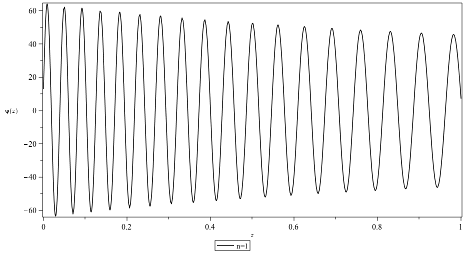
Figure 1: $\psi(z)$ versus $z$ in the radiation-dominated epoch for $A=10^{5}$, $k=0$ and $n$= 1.

Figure 2: $\psi(z)$ versus $z$ in the radiation-dominated epoch for $A=10^{5}$, $k=0$ and $1.1\leq n\leq 2$.

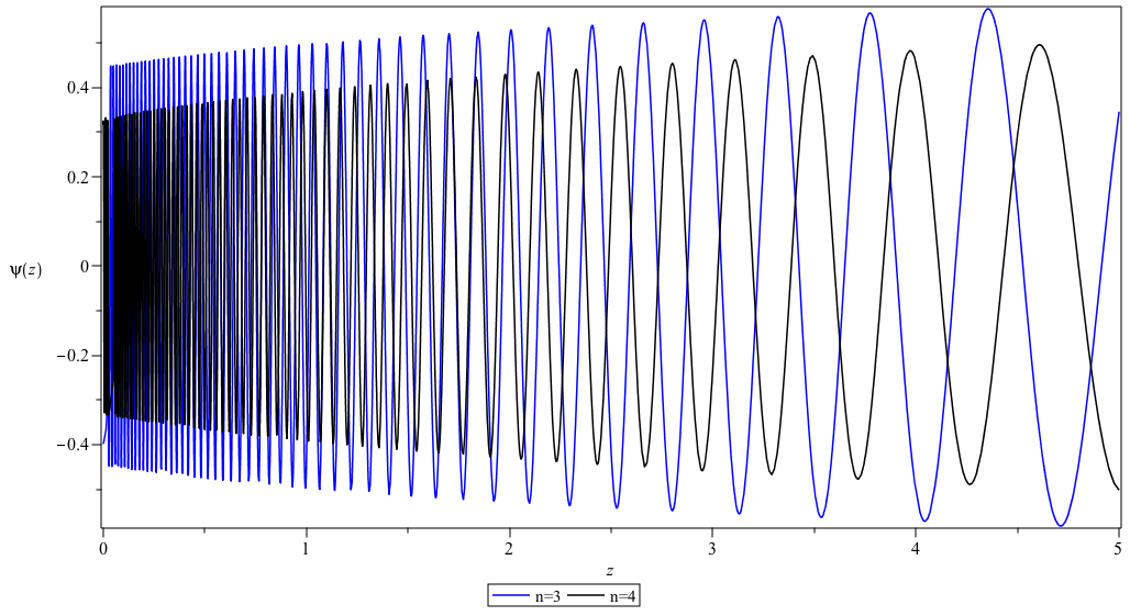
Figure 3: $\psi(z)$ versus $z$ in the radiation-dominated epoch for $A=10^{5}$, $k=0$ and $n\geq 3$.

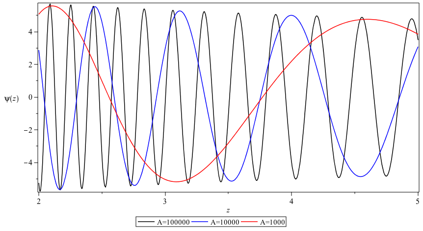
Figure 4: $\psi(z)$ versus $z$ in the radiation-dominated epoch for $n=1.3$, $k=0$.

For the case when $k=1$

For the case when $k=1$, Eq. (37) is written as

$$\psi^{\prime\prime}+\dfrac{2}{(1+z)}\psi^{\prime}+\frac{A}{(1+z)^{4}}(-1-U(z))\psi=0\;,$$ (53)

and for $n=1$, the general solution is a combination of Whittaker functions

$$\psi(z)=C_{3}\mathcal{Y}_{1}\Big{(}0,\frac{\sqrt{1-A}}{2},\frac{2\sqrt{A}}{(1+z)}\Big{)}+C_{4}\mathcal{Y}_{2}\Big{(}0,\frac{\sqrt{1-A}}{2},\frac{2\sqrt{A}}{(1+z)}\Big{)}\;.$$ (54)

We present the numerical solutions for different values of $n$ in the following Figs. 6 - 8. We noticed the oscillatory behaviour for $n=1$ only when the range of redshift begins at $z\geq 0.69$ as shown in Fig. 6. While for values of $1<n\leq 2$, oscillations observed only when the range of redshift begins at $z\geq 1$ as shown in Figs. 6 and 8. From Fig. 6, the rate of the oscillations and the amplitudes or the probabilities of finding a galaxy of mass $A=10^{5}$, are all decreasing with increasing the values of $n$. For $n\geq 3$, oscillatory behaviour is observed only for small range of the redshift as presented in Fig. 8. We also presented the numerical results for different masses $A$ in Fig. 8.

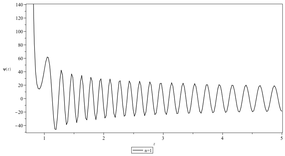
Figure 5: $\psi(z)$ versus $z$ in the radiation-dominated epoch for $A=10^{5}$, $k=1$ and $n=1$.

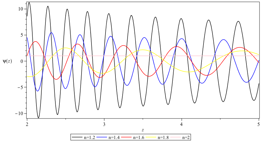
Figure 6: $\psi(z)$ versus $z$ in the radiation-dominated epoch for $A=10^{5}$, $k=1$ and $1<n\leq 2$.

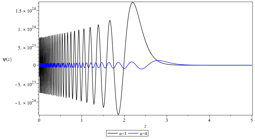
Figure 7: $\psi(z)$ versus $z$ in the radiation-dominated epoch for $A=10^{5}$, $k=1$ and $n\geq 3$.

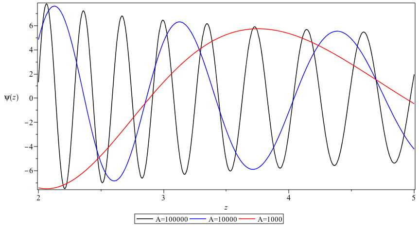
Figure 8: $\psi(z)$ versus $z$ in the radiation-dominated epoch for $k=1$ and $n=1.3$.

For the case when $k=-1$

For the case when $k=-1$, Eq. (37) is written as

$$\psi^{\prime\prime}+\dfrac{2}{(1+z)}\psi^{\prime}+\frac{A}{(1+z)^{4}}(1-U(z))\psi=0\;,$$ (55)

and for $n=1$, the general solution is a combination of Whittaker functions

$$\psi(z)=C_{5}\mathcal{Y}_{1}\Big{(}0,\frac{\sqrt{1-A}}{2},\frac{2I\sqrt{A}}{(1+z)}\Big{)}+C_{6}\mathcal{Y}_{2}\Big{(}0,\frac{\sqrt{1-A}}{2},\frac{2I\sqrt{A}}{(1+z)}\Big{)}\;.$$ (56)

We present the numerical solutions for $k=-1$ and different values of $n$ in the following Figs. 10 - 10.

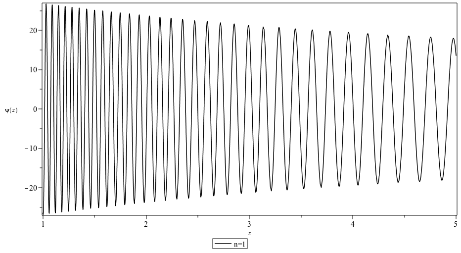
Figure 9: $\psi(z)$ versus $z$ in the radiation-dominated epoch for $A=10^{5}$, $k=-1$ and $n=1$.

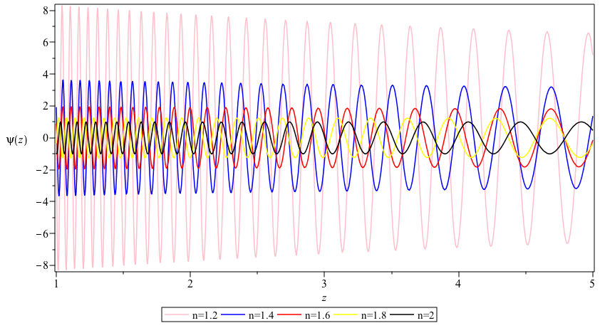
Figure 10: $\psi(z)$ versus $z$ in the radiation-dominated epoch for $A=10^{5}$, $k=-1$ and $1.1\leq n\leq 2$.

4.2 Solutions for the matter-dominated era

In this subsection, we get the solution for the the Schrödinger equation Eq. (37) in the matter-dominated era. From the expressions for the expansion, the Ricci scalar and the effective matter energy density Eqs. (45)-(46), we get

$$\dfrac{\theta f^{\prime\prime}\dot{R}}{f^{\prime}}=\dfrac{-9H^{2}(n-1)}{n}\;,$$ (57)

$$\dfrac{1}{f^{\prime}}(Rf^{\prime}-f)=\dfrac{3H^{2}(n-1)(4n-3)}{n^{2}}\;,$$ (58)

$$\dfrac{\rho_{d}}{f^{\prime}}=\dfrac{3H^{2}(-16n^{2}+26n-6)}{4n^{2}}\;.$$ (59)

Therefore, the Schrödinger equation Eq. (37)

$$U(z)=\dfrac{-2n^{2}}{9(1+z)^{2-3/n}}\Big{(}\dfrac{(-16n^{2}+26n-6)}{2n^{2}}+\dfrac{(n-1)(4n-3)}{n^{2}}+\dfrac{6(n-1)}{n}\Big{)}\;.$$

For the case when $k=0$

For the case when $k=0$, Eq. (37) is written as

$$\psi^{\prime\prime}+\dfrac{2}{(1+z)}\psi^{\prime}-\frac{A}{(1+z)^{4}}U(z)\psi=0\;,$$ (60)

the general solution is combination for Hypergeometric functions

$$\psi(z)=C_{1}\mathcal{H}\Big{(}[],[\dfrac{(3n-3)}{(4n-3)}],\dfrac{An^{2}B(1+z)^{\frac{-4n+3}{n}}}{(4n-3)^{2}}\Big{)}$$

$$+C_{2}\dfrac{1}{(1+z)}\mathcal{H}\Big{(}[],[\dfrac{(5n-3)}{(4n-3)}],\dfrac{An^{2}B(1+z)^{\frac{-4n+3}{n}}}{(4n-3)^{2}}\Big{)}\;,$$ (61)

where $B=\dfrac{-2n^{2}}{9}\Big{(}\dfrac{(-16n^{2}+26n-6)}{2n^{2}}+\dfrac{(n-1)(4n-3)}{n^{2}}+\dfrac{6(n-1)}{n}\Big{)}\;.$
For $n=1$, we get the general solution as a combination of Bessel functions as

$$\psi(z)=\dfrac{C_{1}J_{\nu}(a)(1,\dfrac{4\sqrt{A}}{3\sqrt{1+z}})}{\sqrt{(1+z)}}+\dfrac{C_{2}Y_{\nu}(a)(1,\dfrac{4\sqrt{A}}{3\sqrt{1+z}})}{\sqrt{(1+z)}}\;.$$ (62)

This solution corresponds to the solution found in [13], for the dust case where the cosmological constant was considered to be $\Lambda=0$. We set the initial conditions, $\psi(z_{in})=10^{-3}$ and $\psi^{\prime}(z_{in})=10^{-3}$, where $z_{in}=1100$. The results are presented in Figs. 12 - 14 for a specific choice of the mass $A=10^{5}$ and for different values of $n$. Fig. 12, presents the GR results for $n=1$. The probabilities of finding a galaxy of mass $A=10^{5}$ are slightly increasing with decreasing the redshift (the amplitudes or the probabilities are approximately constant for most of the cycles) for values of $1\leq n\leq 1.5$ see Fig. 12, while the probabilities are decreasing with decreasing the redshift for $n\geq 1.6$ as shown in Fig. 14.

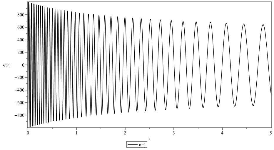
Figure 11: $\psi(z)$ versus $z$ in the matter-dominated era for $A=10^{5}$ and $k=0$.

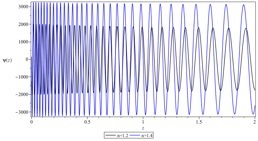
Figure 12: $\psi(z)$ versus $z$ in the matter-dominated era for $A=10^{5}$ $n>1$ and $k=0$.

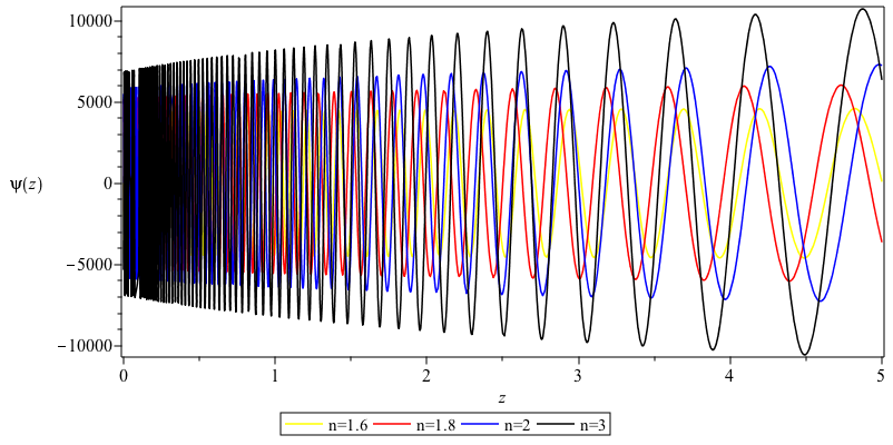
Figure 13: $\psi(z)$ versus $z$ in the matter-dominated era for $A=10^{5}$ $n>1.5$ and $k=0$.

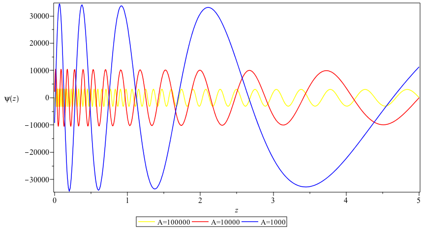
Figure 14: $\psi(z)$ versus $z$ in the matter-dominated era for $n=1.3$ and $k=0$.

For the case when $k=1$

For the case when $k=1$, Eq. (37) is written as

$$\psi^{\prime\prime}+\dfrac{2}{(1+z)}\psi^{\prime}+\frac{A}{(1+z)^{4}}(-1-U(z))\psi=0\;,$$ (63)

and for $n=1$, the general solution is a combination of Whittaker functions

$$\psi(z)=C_{3}\mathcal{Y}_{1}\Big{(}\frac{2\sqrt{A}}{9},\frac{1}{2},\frac{2\sqrt{A}}{(1+z)}\Big{)}+C_{4}\mathcal{Y}_{2}\Big{(}\frac{2\sqrt{A}}{9},\frac{1}{2},\frac{2\sqrt{A}}{(1+z)}\Big{)}\;.$$ (64)

We present the numerical solutions in the following Figs. 16 - 18. We noticed the oscillatory behaviour for $n=1$ and $1<n<2$ only when the range of redshift begins at $z\geq 2$ as shown in Figs. 16 - 16. While for values of $n\geq 1.4$, oscillations observed only when the range of redshift begins at $0<z\geq 2$ as shown in Fig. 18. We also presented the numerical results for different masses $A$ in Fig. 18

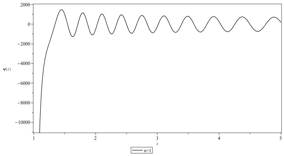
Figure 15: $\psi(z)$ versus $z$ in the matter-dominated epoch for $A=10^{5}$, $k=1$ and $n=1$.

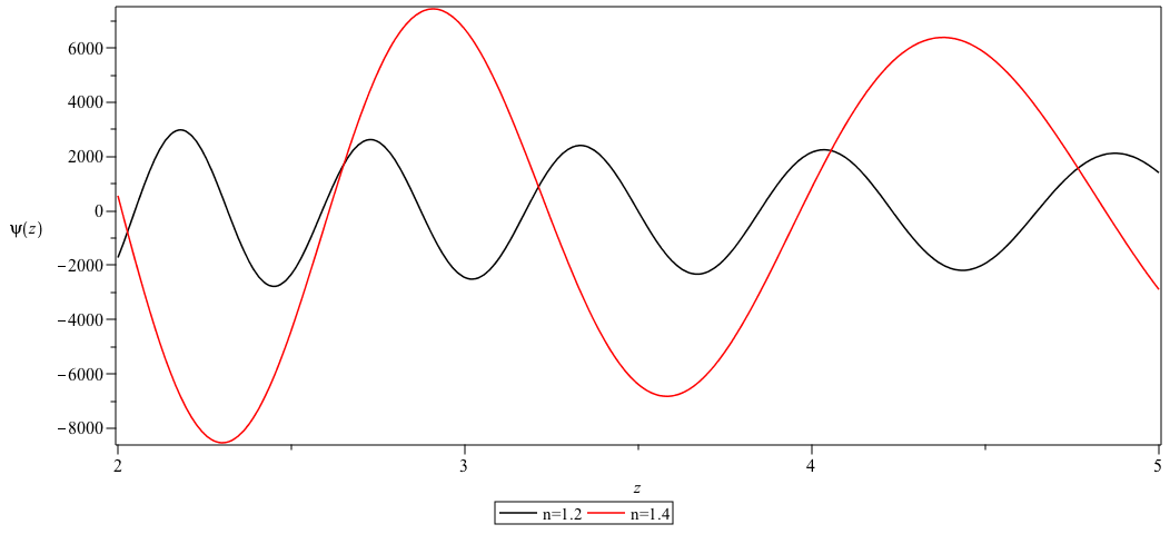
Figure 16: $\psi(z)$ versus $z$ in the matter-dominated epoch for $A=10^{5}$, $k=1$ and $1\leq n<2$.

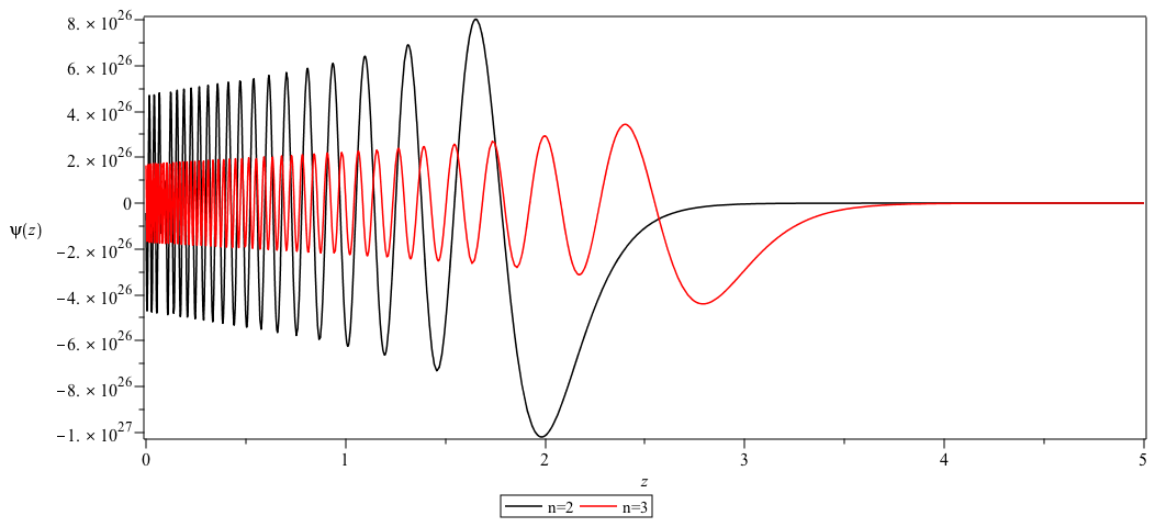
Figure 17: $\psi(z)$ versus $z$ in the matter-dominated epoch for $A=10^{5}$, $k=1$ and $n\geq 2$.

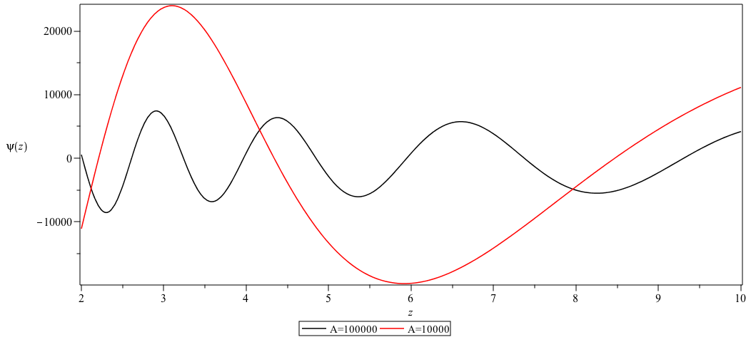
Figure 18: $\psi(z)$ versus $z$ in the matter-dominated epoch for $k=1$ and $n=1.3$.

For the case when $k=-1$

For the case when $k=-1$, Eq. (37) is written as

$$\psi^{\prime\prime}+\dfrac{2}{(1+z)}\psi^{\prime}+\frac{A}{(1+z)^{4}}(1-U(z))\psi=0\;,$$ (65)

and for $n=1$, the general solution is a combination of Whittaker functions

$$\psi(z)=C_{5}\mathcal{Y}_{1}\Big{(}-\frac{2I}{9}\sqrt{A},\frac{1}{2},\frac{2I\sqrt{A}}{(1+z)}\Big{)}+C_{6}\mathcal{Y}_{2}\Big{(}-\frac{2I}{9}\sqrt{A},\frac{1}{2},\frac{2I\sqrt{A}}{(1+z)}\Big{)}\;.$$ (66)

We present the numerical solutions in the following Figs. 20 - 20.

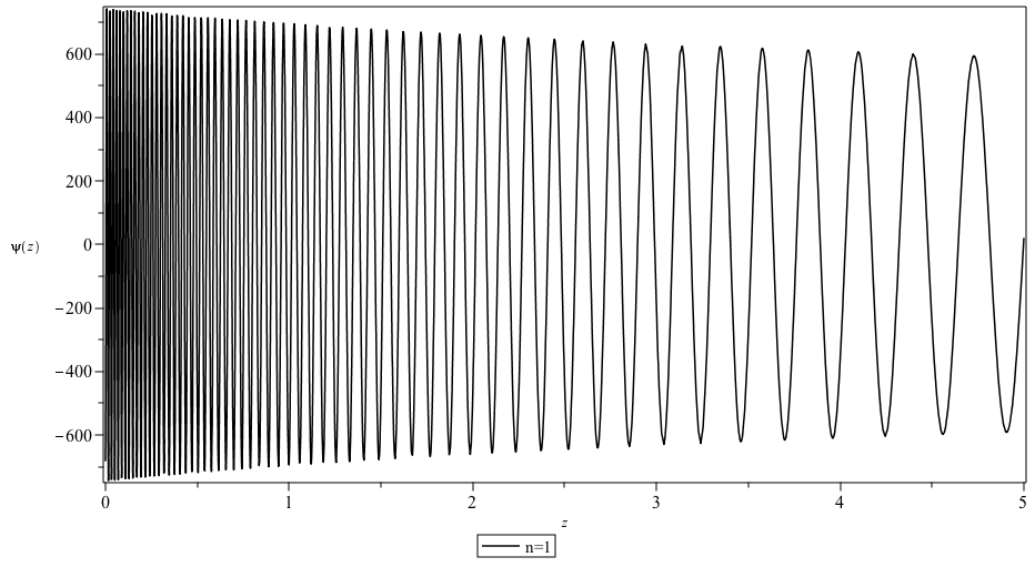
Figure 19: $\psi(z)$ versus $z$ in the matter-dominated epoch for $A=10^{5}$, $k=-1$ and $n=1$.

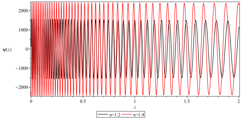
Figure 20: $\psi(z)$ versus $z$ in the matter-dominated epoch for $A=10^{5}$, $k=-1$ and $1\leq n\leq 2$.

5 Conclusions

In this paper, we studied the nature of periodic clustering of large-scale cosmic structures in the context of the $f(R)$ gravity theory. Using the $f(R)$-modified Friedmann equations, we were able to construct the cosmological Schrödinger-like equation. Following similar works in [13] (and references therein), we considered the particle dynamics of galaxies and calculated the probability of finding them at a certain redshift as eigensolutions of Schrödinger equation. We solved the Schrödinger equation for different ranges of $n$ in the $R^{n}$ model for different equation of state parameters (radiation and pure dust). For the radiation- and dust-dominated epochs in the flat universe ($k=0$) case, we got a combination of hypergeometric functions as a general solution of the Schrödinger equation. Some of the specific highlights of this work are as follows: For the radiation- and dust-dominated epochs in the flat universe ($k=0$) and $n=1$, we got a combination of Bessel functions as a general solution (which matches the one for the GR results found in [13] for $\psi(a)$) and as we have shown in Figs. 4, 4, 12 and 14, oscillatory behaviour observed for all values of $n$. However, in the radiation-dominated era, the amplitudes of such oscillations decrease with increasing the values of $n$ as in Figs. 4, 4. For the matter-dominated era, the amplitudes of such oscillations are almost constant for most of the cycles as in Fig. 12. Numerical solutions have been obtained for $k=\pm 1$ cases for both the radiation- and dust-dominated epochs. For instance, for $k=-1$, the cosmological solutions are oscillating functions but they are not periodic oscillations (only for a particular range of the redshift $z$) as in Figs. 6 - 8 and Figs. 16 - 18.
In conclusion, as we have shown in Figs. 4 to 20, for appropriate choices of the initial conditions (and for normalized parameters of the model), a breaking of homogeneity and isotropy indeed occurs on small scales as depicted by the oscillating correlations between galaxies.

References

References

- [1] De Vaucouleurs G 1970 Science 167 1203–1213
- [2] Haggerty M 1970 Physica 50 391–396
- [3] Davis S T 1992 International journal for philosophy of religion 31 13–27
- [4] Wesson P S 1975 Astrophysics and Space Science 32 315–330
- [5] Wesson P S 1978 Astrophysics and Space Science 54 489–495
- [6] Friedman A 1922 Zeitschrift für Physik 10 377–386
- [7] Morikawa M 1990 The Astrophysical Journal 362 L37–L39
- [8] Morikawa M 1991 The Astrophysical Journal 369 20–29
- [9] Broadhurst T J, Ellis R S, Koo D and Szalay A 1990 Nature 343 726–728
- [10] Durrer R and Laukenmann J 1996 Classical and Quantum Gravity 13 1069
- [11] Namane N, Sami H and Abebe A 2018 arXiv preprint arXiv:1807.11330
- [12] Namane N 2018 Studies in Quantum Cosmology Master’s thesis North-West University, South Africa
- [13] Capozziello S, Feoli A and Lambiase G 2000 International Journal of Modern Physics D 9 143–154
- [14] Rosen N 1993 International Journal of Theoretical Physics 32 1435–1440
- [15] Tifft W G 1976
- [16] Joras S E 2011 Some remarks on theories of gravity International Journal of Modern Physics: Conference Series vol 3 (World Scientific) pp 36–47
- [17] Sotiriou T P 2006 Classical and Quantum Gravity 23 5117
- [18] Sotiriou T P and Faraoni V 2010 Reviews of Modern Physics 82 451
- [19] Sotiriou T P 2007 arXiv preprint arXiv:0710.4438
- [20] Clifton T, Ferreira P G, Padilla A and Skordis C 2012 Physics Reports 513 1–189
- [21] Vitagliano V, Sotiriou T P and Liberati S 2010 Physical Review D 82 084007
- [22] Capozziello S and De Laurentis M 2011 Physics Reports 509 167–321
- [23] Busarello G, Capozziello S, De Ritis R, Longo G, Rifatto A, Rubano C and Scudellaro P 1994 Astronomy and Astrophysics 283 717
- [24] Carloni S, Dunsby P K, Capozziello S and Troisi A 2005 Classical and Quantum Gravity 22 4839