Mining Interpretable Spatio-temporal Logic Properties for Spatially Distributed Systems

Abstract

The Internet-of-Things, complex sensor networks, multi-agent cyber-physical systems are all examples of spatially distributed systems that continuously evolve in time. Such systems generate huge amounts of spatio-temporal data, and system designers are often interested in analyzing and discovering structure within the data. There has been considerable interest in learning causal and logical properties of temporal data using logics such as Signal Temporal Logic (STL); however, there is limited work on discovering such relations on spatio-temporal data. We propose the first set of algorithms for unsupervised learning for spatio-temporal data. Our method does automatic feature extraction from the spatio-temporal data by projecting it onto the parameter space of a parametric spatio-temporal reach and escape logic (PSTREL). We propose an agglomerative hierarchical clustering technique that guarantees that each cluster satisfies a distinct STREL formula. We show that our method generates STREL formulas of bounded description complexity using a novel decision-tree approach which generalizes previous unsupervised learning techniques for Signal Temporal Logic. We demonstrate the effectiveness of our approach on case studies from diverse domains such as urban transportation, epidemiology, green infrastructure, and air quality monitoring.

Keywords Distributed systems  $\cdot$ Unsupervised learning  $\cdot$ Spatio-temporal data  $\cdot$ Interpretability  $\cdot$ Spatio-temporal reach and escape logic.

1 Introduction

Due to rapid improvements in sensing and communication technologies, embedded systems are now often spatially distributed. Such spatially distributed systems (SDS) consist of heterogeneous components embedded in a specific topological space, whose time-varying behaviors evolve according to complex mutual inter-dependence relations Nenzi et al. (2018). In the formal methods community, tremendous advances have been achieved for verification and analysis of distributed systems. However, most formal techniques abstract away the specific spatial aspects of distributed systems, which can be of crucial importance in certain applications. For example, consider the problem of developing a bike-sharing system (BSS) in a “sharing economy.” Here, the system consists of a number of bike stations that would use sensors to detect the number of bikes present at a station, and use incentives to let users return bikes to stations that are running low. The bike stations themselves could be arbitrary locations in a city, and the design of an effective BSS would require reasoning about the distance to nearby locations, and the time-varying demand or supply at each location. For instance, the property “there is always a bike and a slot available at distance d from a bike station” depends on the distance of the bike station to its nearby stations. Evaluating whether the BSS functions correctly is a verification problem where the specification is a spatio-temporal logic formula. Similarly, consider the problem of coordinating the movements of multiple mobile robots, or a HVAC controller that activates heating or cooling in parts of a building based on occupancy. Given spatio-temporal execution traces of nodes in such systems, we may be interested in analyzing the data to solve several classical formal methods problems such as fault localization, debugging, invariant generation or specification mining. It is increasingly urgent to formulate methods that enable reasoning about spatially-distributed systems in a way that explicitly incorporates their spatial topology.

In this paper, we focus on one specific aspect of spatio-temporal reasoning: mining interpretable logical properties from data in an SDS. We model a SDS as a directed or undirected graph where individual compute nodes are vertices, and edges model either the connection topology or spatial proximity. In the past, analytic models based on partial differential equations (e.g. diffusion equations) Fiedler and Scheel (2003) have been used to express the spatio-temporal evolution of these systems. While such formalisms are incredibly powerful, they are also quite difficult to interpret. Traditional machine learning (ML) approaches have also been used to uncover the structure of such spatio-temporal systems, but these techniques also suffer from the lack of interpretability. Our proposed method draws on a recently proposed logic known as Spatio-Temporal Reach and Escape Logic (STREL) Bartocci et al. (2017). Recent research on STREL has focused on efficient algorithms for runtime verification and monitoring of STREL specifications Bartocci et al. (2017, 2020). However, there is no existing work on mining STREL specifications.

Mined STREL specifications can be useful in many different contexts in the design of spatially distributed systems; an incomplete list of usage scenarios includes the following applications: (1) Mined STREL formulas can serve as spatio-temporal invariants that are satisfied by the computing nodes, (2) STREL formulas could be used by developers to characterize the properties of a deployed spatially distributed system, which can then be used to monitor any subsequent updates to the system, (3) Clustering nodes that satisfy similar STREL formulas can help debug possible bottlenecks and violations in communication protocols in such distributed systems.

There is considerable amount of recent work on learning temporal logic formulas from data M. Vazquez-Chanlatte et al. (2017); Jin et al. (2015); Mohammadinejad et al. (2020a, b). In particular, the work in this paper is closest to the work on unsupervised clustering of time-series data using Signal Temporal Logic M. Vazquez-Chanlatte et al. (2017). In this work, the authors assume that the user provides a Parametric Signal Temporal Logic (PSTL) formula, and the procedure projects given temporal data onto the parameter domain of the PSTL formula. The authors use off-the-shelf clustering techniques to group parameter values and identify STL formulas corresponding to each cluster. There are a few hurdles in applying such an approach to spatio-temporal data. First, in M. Vazquez-Chanlatte et al. (2017), the authors assume a monotonic fragment of PSTL: there is no such fragment identified in the literature for STREL. Second, in M. Vazquez-Chanlatte et al. (2017), the authors assume that clusters in the parameter space can be separated by axis-aligned hyper-boxes. Third, given spatio-temporal data, we can have different choices to impose the edge relation on nodes, which can affect the formula we learn.

To address the shortcomings of previous techniques, we introduce PSTREL, by treating threshold constants in signal predicates, time bounds in temporal operators, and distance bounds in spatial operators as parameters. We then identify a monotonic fragment of PSTREL, and propose a multi-dimensional binary-search based procedure to infer tight parameter valuations for the given PSTREL formula. We also explore the space of implied edge relations between spatial nodes, proposing an algorithm to define the most suitable graph. After defining a projection operator that maps a given spatio-temporal signal to parameter values of the given PSTREL formula, we use an agglomerative hierarchical clustering technique to cluster spatial locations into hyperboxes. We improve the method of M. Vazquez-Chanlatte et al. (2017) by introducing a decision-tree based approach to systematically split overlapping hyperbox clusters. The result of our method produces axis-aligned hyperbox clusters that can be compactly described by an STREL formula that has length proportional to the number of parameters in the given PSTREL formula (and independent of the number of clusters). Finally, we give human-interpretable meanings for each cluster. We show the usefulness of our approach considering four benchmarks: COVID-19 data from LA County, Outdoor air quality data, BSS data and movements of the customer in a Food Court.

Running Example: A Bike Sharing System (BSS)

To ease the exposition of key ideas in the paper, we use an example of a BSS deployed in the city of Edinburgh, UK. The BSS consists of a number of bike stations, distributed over a geographic area. Each station has a fixed number of bike slots. Users can pick up a bike, use it for a while, and then return it to another station in the area. The data that we analyze are the number of bikes (B) and empty slots (S) at each time step in each bike station. With the advent of electric bikes, BSS have become an important aspect in urban mobility, and such systems make use of embedded devices for diverse purposes such as tracking bike usage, billing, and displaying information about availability to users over apps. Fig. 1b shows the map of the Edinburgh city with the bike stations. Different colors of the nodes represent different learned clusters as can be seen in Fig. 1a. For example, using our approach, we learn that stations in orange cluster have a long wait time, and stations in red cluster are the most undesirable stations as they have long wait time and do not have nearby stations with bike availability. If we look at the actual location of red points in Fig. 1b, they are indeed far away stations.

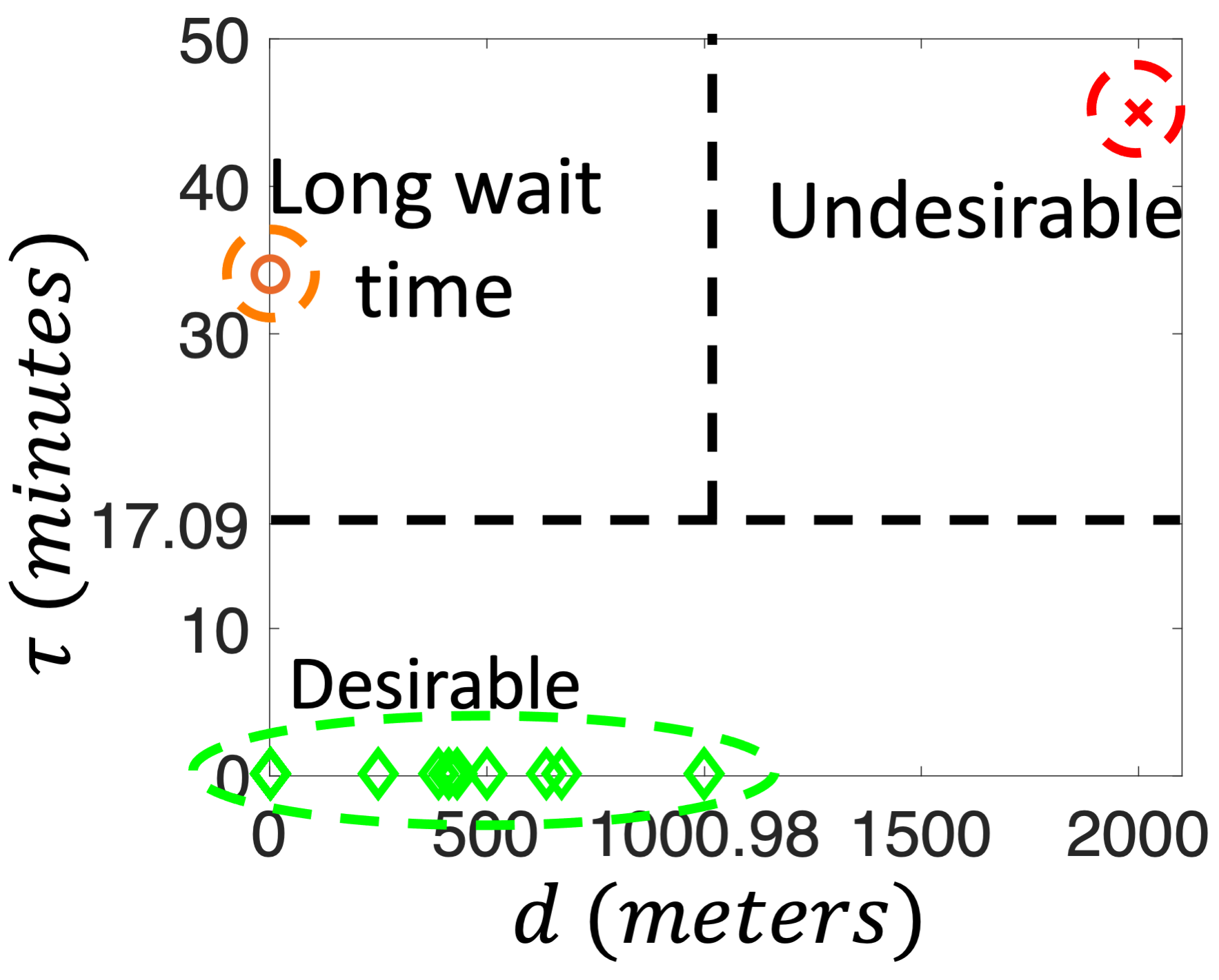
(a) Clusters learned

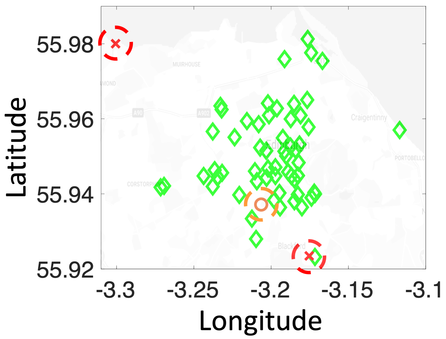
(b) BSS locations in Edinburgh

Figure 1: Interpretable clusters automatically identified by our technique.

2 Background

In this section, we introduce the notation and terminology for spatial models and spatio-temporal traces and we describe Spatio-Temporal Reach and Escape Logic (STREL).

Definition 1 (Spatial Model)

A spatial model $\mathcal{S}$ is defined as a pair $\langle L,W\rangle$, where $L$ is a set of nodes or locations and $W\subseteq L\times\mathbb{R}\times L$ is a nonempty relation associating each distinct pair $\ell_{1},\ell_{2}\in L$ with a label $w\in\mathbb{R}$ (also denoted $\ell_{1}\xrightarrow{w}\ell_{2}$).

There are many different choices possible for the proximity relation $W$; for example, $W$ could be defined in a way that the edge-weights indicate spatial proximity, communication network connectivity etc. Given a set of locations, unless there is a user-specified $W$, we note that there are several graphs (and associated edge-weights) that we can use to express spatial models. We explore these possibilities in Sec. 3. For the rest of this section, we assume that $W$ is defined using the notion of $(\delta,d)$-connectivity graph as defined in Definition 2.

Definition 2 ($(\delta,d)$-connectivity spatial model)

Given a compact metric space $M$ with the distance metric $d:M\times M\to\mathbb{R}^{\geq 0}$, a set of locations $L$ that is a finite subset of $M$, and a fixed $\delta\in\mathbb{R},\delta>0$, a $(\delta,d)$-connectivity spatial model is defined as $\langle L,W\rangle$, where $(\ell_{1},w,\ell_{2})\in W$ iff $d(\ell_{1},\ell_{2})=w$, and $w<\delta$.

Example 1

In the BSS, each bike station is a node/location in the spatial model, where locations are assumed to lie on the metric space defined by the 3D spherical manifold of the earth’s surface; each location is defined by its latitude and longitude, and the distance metric is the Haversine distance. Fig. 2b shows the $\delta$-connectivity graph of the Edinburgh BSS, with $\delta=1km$.

Definition 3 (Route)

For a spatial model $\mathcal{S}=\langle L,W\rangle$, a route $\tau$ is an infinite sequence $\ell_{0}\ell_{1}\cdots\ell_{k}\cdots$ such that for any $i\geq 0$, $\ell_{i}\xrightarrow{w_{i}}\ell_{i+1}$.

For a route $\tau$, $\tau[i]$ denotes the $i^{th}$ node $\ell_{i}$ in $\tau$, $\tau[i..]$ indicates the suffix route $\ell_{i}\ell_{i+1}...$, and $\tau(\ell)$ denotes $\min{i\mid\tau[i]=\ell}$, i.e. the first occurrence of $\ell$ in $\tau$. Note that $\tau(\ell)=\infty$ if $\forall i\tau[i]\neq\ell$. We use $\mathcal{T}(\mathcal{S})$ to denote the set of routes in $\mathcal{S}$, and $\mathcal{T}(\mathcal{S},\ell)$ to denote the set of routes in $\mathcal{S}$ starting from $\ell\in L$. We can use routes to define the route distance between two locations in the spatial model as follows.

Definition 4 (Route Distance and Spatial Model Induced Distance)

Given a route $\tau$, the route distance along $\tau$ up to a location $\ell$ denoted $d_{\mathcal{S}}^{\tau}(\ell)$ is defined as $\sum_{i=0}^{\tau(\ell)}w_{i}$. The spatial model induced distance between locations $\ell_{1}$ and $\ell_{2}$ (denoted $d_{\mathcal{S}}(\ell_{1},\ell_{2})$) is defined as: $d_{\mathcal{S}}(\ell_{1},\ell_{2})=\min_{\tau\in\mathcal{T}(\mathcal{S},\ell_{1})}d_{\mathcal{S}}^{\tau}(\ell_{2})$.

Note that by the above definition, $d_{\mathcal{S}}^{\tau}(\ell)=0$ if $\tau[0]=\ell$ and $\infty$ if $\ell$ is not a part of the route (i.e. $\tau(\ell)=\infty$), and $d_{\mathcal{S}}(\ell_{1},\ell_{2})=\infty$ if there is no route from $\ell_{1}$ to $\ell_{2}$.

Spatio-temporal Time-Series.  A spatio-temporal trace associates each location in a spatial model with a time-series trace. Formally, a time-series trace $x$ is a mapping from a time domain $\mathbb{T}$ to some bounded and non-empty set known as the value domain $\mathcal{V}$. Given a spatial model $\mathcal{S}=\langle L,W\rangle$, a spatio-temporal trace $\sigma$ is a function from $L\times\mathbb{T}$ to $\mathcal{V}$. We denote the time-series trace at location $\ell$ by $\sigma(\ell)$.

Example 2

Consider a spatio-temporal trace $\sigma$ of the BSS defined such that for each location $\ell$ and at any given time $t$, $\sigma(\ell,t)$ is $(B(t),S(t))$, where $B(t)$ and $S(t)$ are respectively the number of bikes and empty slots at time $t$.

2.1 Spatio-Temporal Reach and Escape Logic (STREL)

Syntax.  STREL is a logic that was introduced in Bartocci et al. (2017) as a formalism for monitoring spatially distributed cyber-physical systems. STREL extends Signal Temporal Logic Maler and Nickovic (2004) with two spatial operators, reach and escape, from which is possible to derive other three spatial modalities: everywhere, somewhere and surround. The syntax of STREL is given by:

$$\varphi::=true\mid\mu\mid\neg\varphi\mid\varphi_{1}\wedge\varphi_{2}\mid\varphi_{1}\>\mathrm{U}_{I}\>\varphi_{2}\mid\varphi_{1}\>\mathcal{R}_{D}\>\varphi_{2}\mid\mathcal{E}_{D}\>\varphi.$$

Here, $\mu$ is an atomic predicate (AP) over the value domain $\mathcal{V}$. Negation $\neg$ and conjunction $\wedge$ are the standard Boolean connectives, while $\mathrm{U}_{I}$ is the temporal operator until with $I$ being a non-singular interval over the time-domain $\mathbb{T}$. The operators $\mathcal{R}_{D}$ and $\mathcal{E}_{D}$ are spatial operators where $D$ denotes an interval over the distances induced by the underlying spatial model, i.e., an interval over $\mathbb{R}^{\geq 0}$.

Semantics.  A STREL formula is evaluated piecewise over each location and each time appearing in a given spatio-temporal trace. We use the notation $(\sigma,\ell)\models\varphi$ if the formula $\varphi$ holds true at location $\ell$ for the given spatio-temporal trace $\sigma$. The interpretation of atomic predicates, Boolean operations and temporal operators follows standard semantics for Signal Temporal Logic: E.g., for a given location $\ell$ and a given time $t$, the formula $\varphi_{1}\mathrm{U}_{I}\varphi_{2}$ holds at $\ell$ iff there is some time $t^{\prime}$ in $t\oplus I$ where $\varphi_{2}$ holds, and for all times $t^{\prime\prime}$ in $[t,t^{\prime})$, $\varphi_{1}$ holds. Here the $\oplus$ operator defines the interval obtained by adding $t$ to both interval end-points. We use standard abbreviations $\mathbf{F}_{I}\varphi=\mathit{true}\mathrm{U}_{I}\varphi$ and $\mathbf{G}_{I}\varphi=\neg\mathbf{F}_{I}\varphi$, for the eventually and globally operators. The reachability ($\mathcal{R}_{D}$) and escape ($\mathcal{E}_{D}$)operators are spatial operators. The formula $\varphi_{1}\mathcal{R}_{D}\varphi_{2}$ holds at a location $\ell$ if there is a route $\tau$ starting at $\ell$ that reaches a location $\ell^{\prime}$ that satisfies $\varphi_{2}$, with a route distance $d_{\mathcal{S}}^{\tau}(\ell^{\prime})$ that lies in the interval $D$, and for all preceding locations, including $\ell$, $\varphi_{1}$ holds true. The escape formula $\mathcal{E}_{D}\varphi$ holds at a location $\ell$ if there exists a location $\ell^{\prime}$ at a route distance $d_{\mathcal{S}}(\ell_{1},\ell_{2})$ that lies in the interval $D$ and a route starting at $\ell$ and reaching $\ell^{\prime}$ consisting of locations that satisfy $\varphi$. We define two other operators for notational convenience: The somewhere operator, denoted $\diamonddiamond_{D}\varphi$, is defined as $\mathit{true}\mathcal{R}_{D}\varphi$, and the everywhere operator, denoted $\boxbox_{D}\varphi$ is defined as $\neg\diamonddiamond_{D}\neg\varphi$, their meaning is described in the next example.

Example 3

In the BSS, we use atomic predicates $S>0$ and $B>10$, and the formula $\mathbf{G}_{[0,3\mathrm{hours}]}\diamonddiamond_{[0,1\mathrm{km}]}(B>10)$ is true if always within the next $3$ hours, at a location $\ell$, there is some location $\ell^{\prime}$ at most $1$ km from $\ell$ where, the number of bikes available exceed $10$. Similarly, the formula $\boxbox_{[0,1\mathrm{km}]}\mathbf{G}_{[0,30\mathrm{min}]}(S>0)$ is true at a location $\ell$ if for all locations within $1$km, for the next $30$ mins, there is no empty slot.

3 Constructing a Spatial Model

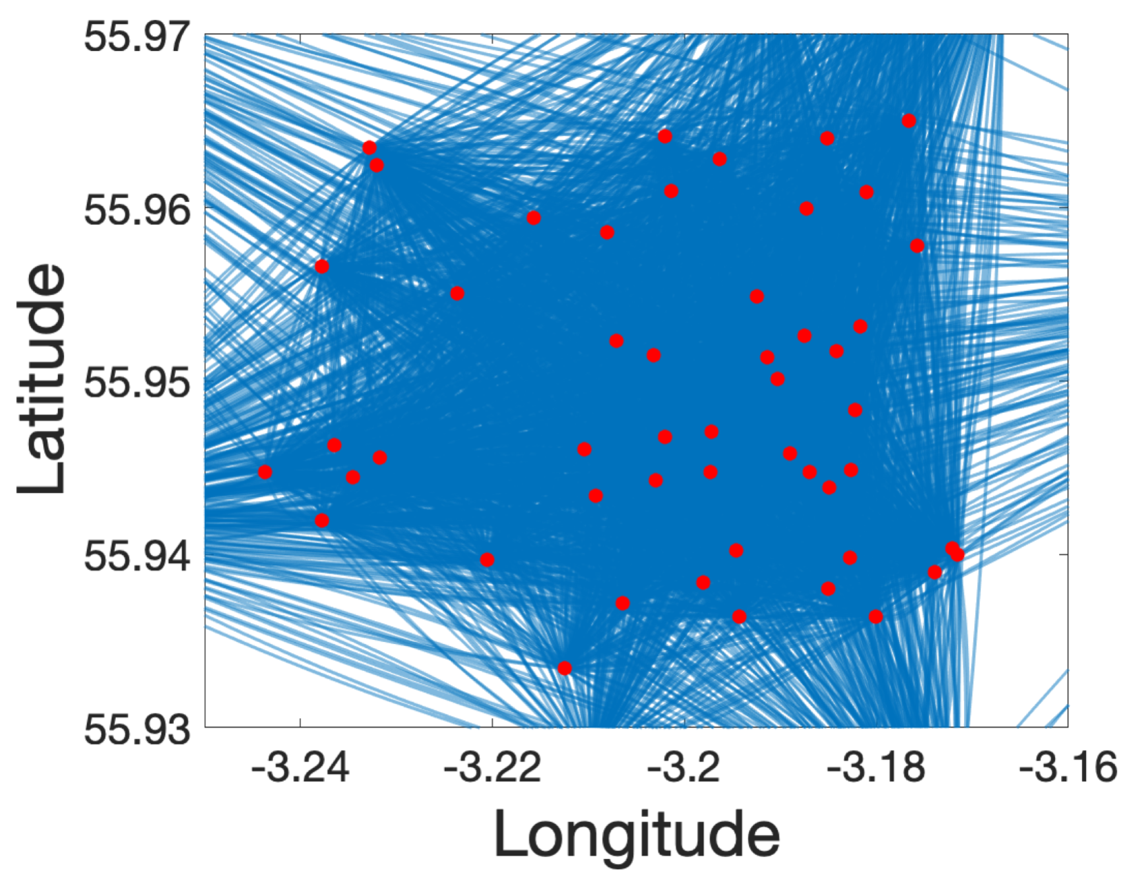
(a)

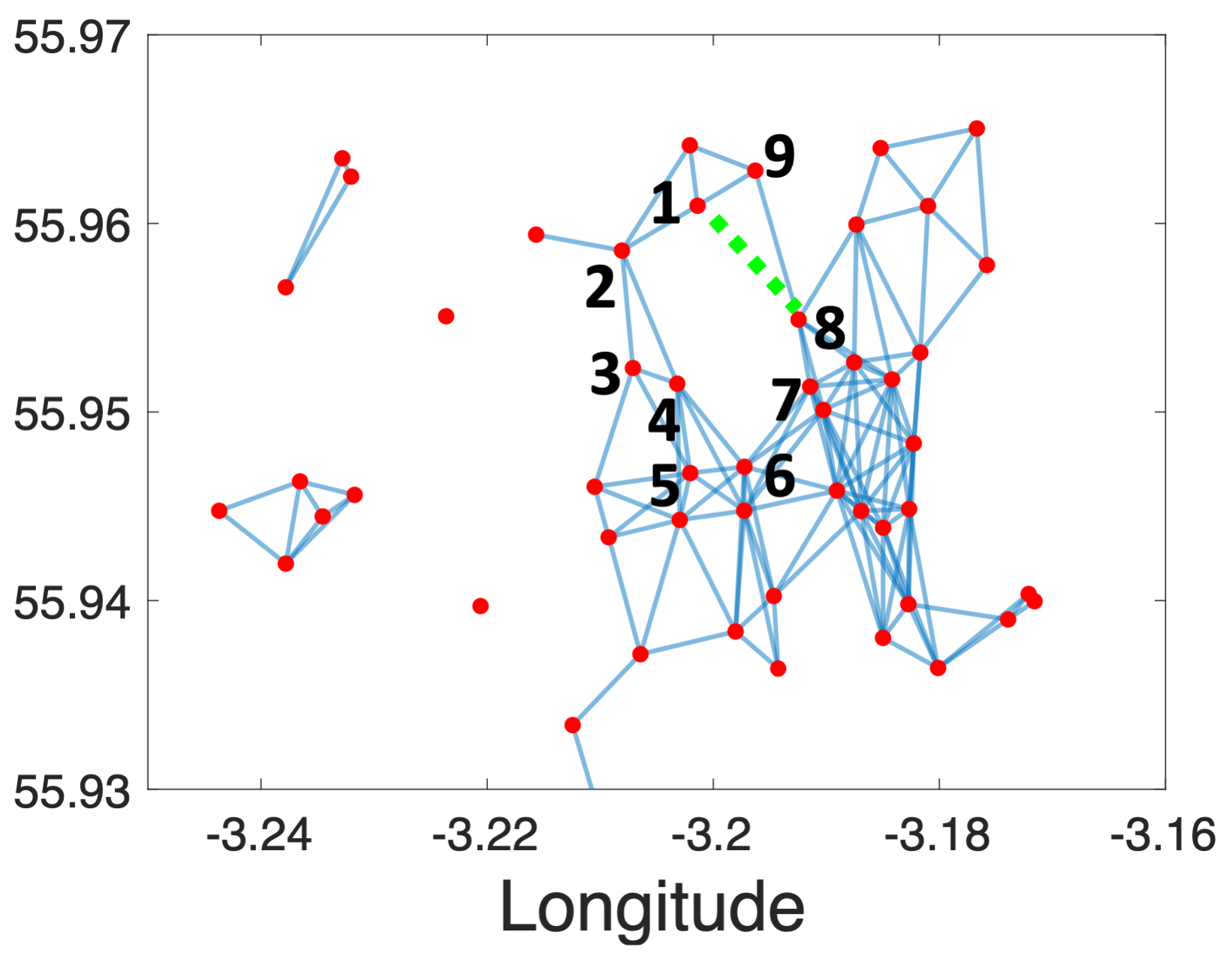
(b)

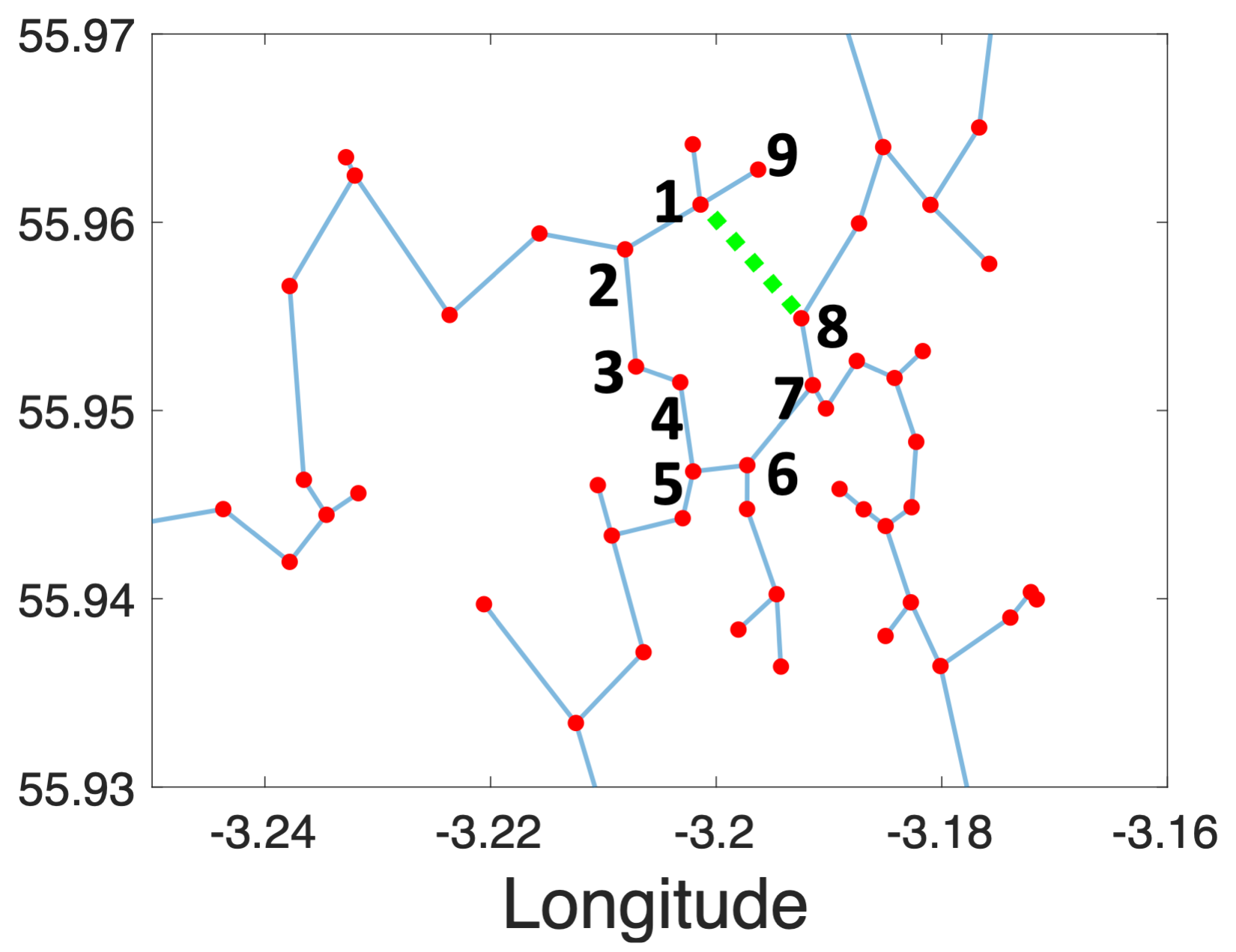
(c)

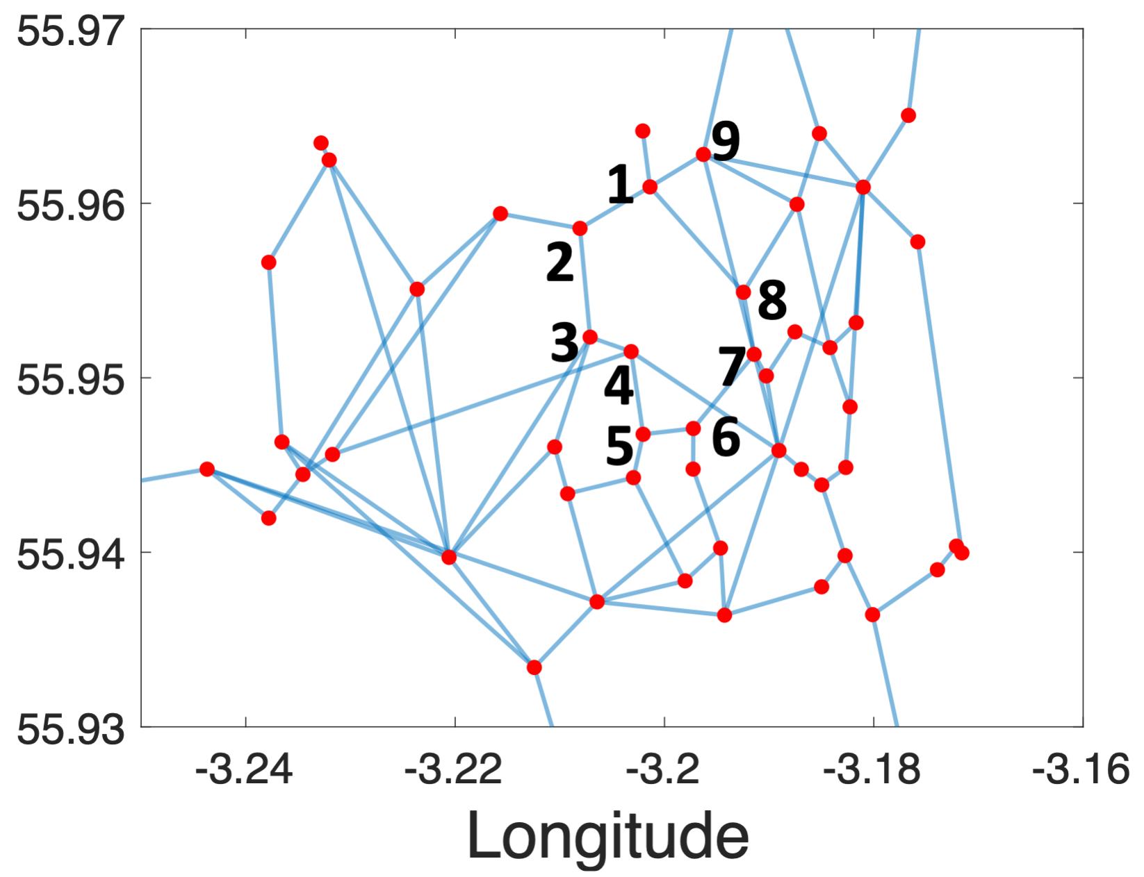
(d)

Figure 2: Different approaches for constructing the spatial model for the BSS. (a) shows an $(\infty,d_{\mathrm{hvrsn}})$-connectivity spatial model where $d_{\mathrm{hvrsn}}$ is the Haversine distance between locations. (b) shows a $(\delta,d_{\mathrm{hvrsn}})$-connectivity spatial model where $\delta=1km$. Observe that the spatial model is disconnected. (c) shows an MST-spatial model. (d) shows an $(\alpha,d_{\mathrm{hvrsn}})$ enhanced MSG spatial model with $\alpha=2$. Observe that this spatial model is sparse compared even to the $(\delta,d_{\mathrm{hvrsn}})$-connectivity spatial model.

In this section, we present four approaches to construct a spatial model, and discuss the pros and cons of each approach.

1. $(\infty,d)$-connectivity spatial model: This spatial model corresponds to the $(\delta,d)$-connectivity spatial model as presented in Definition 2, where we set $\delta=\infty$. We note that this gives us a fully connected graph, i.e. where $|W|$ is $O(|L|^{2})$. We remark that our learning algorithm uses monitoring STREL formulas as a sub-routine, and from Lemma 2 in Appendix, we can see that as the complexity of monitoring a STREL formula is linear in $|W|$, a fully connected graph is undesirable.

2. $(\delta,d)$-connectivity spatial model: This is the model presented in Definition 2, where $\delta$ is heuristically chosen in an application-dependent fashion. Typically, the $\delta$ we choose is much smaller compared to the distance between the furthest nodes in the given topological space. This gives us $W$ that is sparse, and thus with a lower monitoring cost; however, a small $\delta$ can lead to a disconnected spatial model which can affect the accuracy of the learned STREL formulas. Furthermore, this approach may overestimate the spatial model induced distance between two nodes (as in Definition 4) that are not connected by a direct edge. For instance, in Fig. 2b, nodes $1$ and $8$ are connected through the route $1\rightarrow 9\rightarrow 8$, and sum of the edge-weights along this route is larger than the actual (metric) distance of $1$ and $8$.

3. MST-spatial model: To minimize the number of edges in the graph while keeping the connectivity of the graph, we can use Minimum Spanning Tree (MST) as illustrated in Fig. 2c. This gives us $|W|$ that is $O(|L|)$, which makes monitoring much faster, while resolving the issue of disconnected nodes in the $(\delta,d)$-spatial model. However, an MST can also lead to an overestimate of the spatial model induced distance between some nodes in the graph. For example, in Fig. 2c, the direct distance between nodes $1$ and $8$ is much smaller than their route distance (through the route $1\rightarrow 2\rightarrow 3\rightarrow 4\rightarrow 5\rightarrow 6\rightarrow 7\rightarrow 8$).

4. $(\alpha,d)$-Enhanced MSG Spatial Model: To address the shortcomings of previous approaches, we propose constructing a spatial model that we call the $(\alpha,d)$-Enhanced Minimum Spanning Graph Spatial model. First, we construct an MST over the given set of locations and use it to define $W$ and pick $\alpha$ as some number greater than $1$. Then, for each distinct pair of locations $\ell_{1},\ell_{2}$, we compute the shortest route distance $d_{\mathcal{S}}(\ell_{1},\ell_{2})$ between them in the constructed MST, and compare it to their distance $d(\ell_{1},\ell_{2})$ in the metric space. If $d_{\mathcal{S}}(\ell_{1},\ell_{2})>\alpha\cdot d(\ell_{1},\ell_{2})$, then we add an edge $(\ell_{1},d(\ell_{1},\ell_{2}),\ell_{2})$ to $W$. The resulting spatial model is no longer a tree, but typically is still sparse. The complete algorithm, is provided in Algo. 1, which is a simple way of constructing an $(\alpha,d)$-enhanced MSG spatial model, and incurs a one-time cost of $O(|L|^{2}\cdot(|L|+|W|\cdot\log(|L|)))$. We believe that the time complexity can be further improved using a suitable dynamic programming based approach. In our case studies, the cost of building the enhanced MSG spatial model was insignificant compared to the other steps in the learning procedure. The runtimes of our learning approach for different kinds of spatial models on various case studies is illustrated in Table. 1. We also represent information about the number of isolated nodes in each graph. We consider the run-time greater than 30 minutes as time-out. The results demonstrate that $(\infty,d_{\mathrm{hvrsn}})$-connectivity spatial model usually results in time-out because of the large number of edges. While $(\delta,d_{\mathrm{hvrsn}})$-connectivity spatial model results in a better run-time, it has the problem of isolated nodes or dis-connectivity. MST-spatial model neither results in time-out or dis-connectivity; however, it has the problem of overestimating distances between nodes. While our approach, $(\alpha,d_{\mathrm{hvrsn}})$-Enhanced MSG Spatial Model, has a slightly worse run-time compared to MST-spatial model, it improves the distance over-approximation issue.

Case	$(\infty,d_{\mathrm{hvrsn}})-$	$(\delta,d_{\mathrm{hvrsn}})-$	MST	$(\alpha,d_{\mathrm{hvrsn}})-$
	connectivity	connectivity		Enhanced MSG
COVID-19	time-out,0	1007.44s,75	600.89s,0	813.65s,0
BSS	time-out,0	934.41s,17	519.30s,0	681.78s,0
Air Quality	time-out,0	111.36s,46	119.94s,0	136.02s,0
Food Court	170.62s,0	84.25s,0	73.53s,0	78.24s,0

Table 1: Run time of the learning algorithm (seconds), number of isolated nodes in the spatial model . , . (threshold for time-out is set to 30 minutes).

Input: A set of locations $L$ (vertices of the graph), Longitudes and Latitudes of the locations, factor $\alpha>1$

Output: $\mathcal{S}$

$\mathcal{S}=minSpanningTree(L,\mathsf{Longitudes},\mathsf{Latitudes})$// Prim’s algorithm

1

2 for $i\leftarrow 1$ to $|L|$ do

3       for $j\leftarrow i+1$ to $|L|$ do

             // Length of the shortest path between i and j

4             $shortestPathMST_{ij}=length(shortestPath(\mathcal{S},i,j))$

             // Compute the Haversine distance between i and j

5             $\mathsf{directDistance}_{ij}=d_{\mathrm{hvrsn}}(\mathsf{longitudes}[i,j],\mathsf{latitudes}[i,j])$

6             if $shortestPathMST_{ij}>\alpha\cdot directDistance_{ij}$ then  $addEdge(\mathcal{S},i,j)$

7            

8      

return $\mathcal{S}$

Algorithm 1 Algorithm to create an $(\alpha,d_{\mathrm{hvrsn}})$-Enhanced MSG Spatial Model

4 Learning STREL formulas from data

In this section, we first introduce Parametric Spatio-Temporal Reach and Escape Logic (PSTREL) and the notion of monotonicity for PSTREL formulas. Then, we introduce a projection function $\pi$ that maps a spatio-temporal trace to a valuation in the parameter space of a given PSTREL formula. We then cluster the trace-projections using Agglomerative Hierarchical Clustering, and finally learn a compact STREL formula for each cluster using Decision Tree techniques.

Parametric STREL (PSTREL).  Parametric STREL (PSTREL) is a logic obtained by replacing one or more numeric constants appearing in STREL formulas by parameters; parameters appearing in atomic predicates are called magnitude parameters $\mathcal{P}_{\mathcal{V}}$, and those appearing in temporal and spatial operators are called timing $\mathcal{P}_{\mathbb{T}}$ and spatial parameters $\mathcal{P}_{d_{\mathcal{S}}}$ respectively. Each parameter in $\mathcal{P}_{\mathcal{V}}$ take values from $\mathcal{V}$, those in $\mathcal{P}_{\mathbb{T}}$ take values from $\mathbb{T}$, and those in $\mathcal{P}_{d_{\mathcal{S}}}$ take values from $\mathbb{R}^{\geq 0}$ (i.e. the set of values that the $d_{\mathcal{S}}$ metric can take for a given spatial model). We define a valuation function $\nu$ that maps all parameters in a PSTREL formula to their respective values.

Example 4

Consider the PSTREL versions of the STREL formulas introduced in Example 3 $\varphi(\mathbf{p}_{\tau},\mathbf{p}_{d},\mathbf{p}_{c})$ = $\mathbf{G}_{[0,\mathbf{p}_{\tau}]}\diamonddiamond_{[0,\mathbf{p}_{d}]}(B>\mathbf{p}_{c})$. The valuation $\nu$: $\mathbf{p}_{\tau}\mapsto 3\mathrm{hours}$, $\mathbf{p}_{d}\mapsto 1\mathrm{km}$, and $\mathbf{p}_{c}\mapsto 10$ returns the STREL formula introduced in Example 3.

Definition 5 (Parameter Polarity, Monotonic PSTREL)

A polarity function $\gamma$ maps a parameter to an element of $\{+,-\}$, and is defined as follows:

$\displaystyle\begin{aligned} \gamma(\mathbf{p})&=+\ \ \mathrel{\stackrel{{\scriptstyle\makebox[0.0pt]{\mbox{def}}}}{{=}}}\ \ \nu^{\prime}(\mathbf{p})>\nu(\mathbf{p})\wedge(\sigma,\ell)\models\varphi(\nu(\mathbf{p}))\Rightarrow(\sigma,\ell)\models\varphi(\nu^{\prime}(\mathbf{p}))\\ \gamma(\mathbf{p})&=-\ \ \mathrel{\stackrel{{\scriptstyle\makebox[0.0pt]{\mbox{def}}}}{{=}}}\ \ \nu^{\prime}(\mathbf{p})<\nu(\mathbf{p})\wedge(\sigma,\ell)\models\varphi(\nu(\mathbf{p}))\Rightarrow(\sigma,\ell)\models\varphi(\nu^{\prime}(\mathbf{p}))\\ \end{aligned}$

The monotonic fragment of PSTREL consists of PSTREL formulas where all parameters have either positive or negative polarity.

In simple terms, the polarity of a parameter $\mathbf{p}$ is positive if it is easier to satisfy $\varphi$ as we increase the value of $\mathbf{p}$ and is negative if it is easier to satisfy $\varphi$ as we decrease the value of $\mathbf{p}$. The notion of polarity for PSTL formulas was introduced in Asarin et al. (2011), and we extend this to PSTREL and spatial operators. The polarity for PSTREL formulas $\varphi(d_{1},d_{2})$ of the form $\diamonddiamond_{[d_{1},d_{2}]}\psi$, $\psi_{1}\mathcal{R}_{[d_{1},d_{2}]}\psi_{2}$, and $\mathcal{E}_{[d_{1},d_{2}]}\psi$ are $\gamma(d_{1})=-$ and $\gamma(d_{2})=+$, i.e. if a spatio-temporal trace satisfies $\varphi(\nu(d_{1}),\nu(d_{2}))$, then it also satisfies any STREL formula over a strictly larger spatial model induced distance interval, i.e. by decreasing $\nu(d_{1})$ and increasing $\nu(d_{2})$. For a formula $\boxbox_{[d_{1},d_{2}]}\psi$, $\gamma(d_{1})=+$ and $\gamma(d_{2})=-$, i.e. the formula obtained by strictly shrinking the distance interval. The proofs are simple, and provided in Appendix for completeness.

Definition 6 (Validity Domain, Boundary)

Let $P=\mathcal{V}^{|\mathcal{P}_{\mathcal{V}}|}\times\mathbb{T}^{|\mathcal{P}_{\mathbb{T}}|}\times(\mathbb{R}^{\geq 0})^{|\mathcal{P}_{d_{\mathcal{S}}}|}$ denote the space of parameter valuations, then the validity domain $V$ of a PSTREL formula at a location $\ell$ with respect to a set of spatio-temporal traces $\Sigma$ is defined as follows: $V(\varphi(\mathbf{p}),\ell,\Sigma)=\{\nu(\mathbf{p})\mid\mathbf{p}\in P,\sigma\in\Sigma,(\sigma,\ell)\models\varphi(\nu(\mathbf{p}))\}$ The validity domain boundary $\partial V(\varphi(\varphi),\ell,\Sigma)$ is defined as the intersection of $V(\varphi,\ell,\Sigma)$ with the closure of its complement.

Spatio-Temporal Trace Projection.  We now explain how a monotonic PSTREL formula $\varphi(\mathbf{p})$ can be used to automatically extract features from a spatio-temporal trace. The main idea is to define a total order $>_{\mathcal{P}}$ on the parameters $\mathbf{p}$ (i.e. parameter priorities) that allows us to define a lexicographic projection of the spatio-temporal trace $\sigma$ at each location $\ell$ to a parameter valuation $\nu(\mathbf{p})$ (this is similar to assumptions made in Jin et al. (2015); M. Vazquez-Chanlatte et al. (2017)). We briefly remark how we can relax this assumption later. Let $\nu_{j}$ denote the valuation of the $j^{th}$ parameter.

Definition 7 (Parameter Space Ordering, Projection)

A total order on parameter indices $j_{1}>\ldots>j_{n}$ imposes a total order $\prec_{\mathrm{lex}}$ on the parameter space defined as:

$$\nu(\mathbf{p})\prec_{\mathrm{lex}}\nu^{\prime}(\mathbf{p})\Leftrightarrow\exists j_{k}\text{ s.t. }\left\{\begin{array}[]{l}\gamma(\mathbf{p}_{j_{k}})=+\Rightarrow\nu_{j_{k}}<\nu^{\prime}_{j_{k}}\\ \gamma(\mathbf{p}_{j_{k}})=-\Rightarrow\nu_{j_{k}}>\nu^{\prime}_{j_{k}}\end{array}\right.\,\mathrm{and}\ \forall m<_{\mathcal{P}}k,\nu_{m}=\nu^{\prime}_{m}.$$

Given above total order, $\pi_{\mathrm{lex}}(\sigma,\ell)=\inf_{\prec_{\mathrm{lex}}}\{\nu(\mathbf{p})\in\partial V(\varphi(\mathbf{p}),\{\sigma\}\}$.

In simple terms, given a total order on the parameters, the lexicographic projection maps a spatio-temporal trace to valuations that are least permissive w.r.t. the parameter with the greatest priority, then among those valuations, to those that are least permissive w.r.t. the parameter with the next greater priority, and so on. Finding a lexicographic projection can be done by sequentially performing binary search on each parameter dimension M. Vazquez-Chanlatte et al. (2017). It is easy to show that $\pi_{\mathrm{lex}}$ returns a valuation on the validity domain boundary. The method for finding the lexicographic projection is formalized in Algo. 2. The algorithm begins by setting the lower and upper bounds of valuations for each parameter. Then, each parameter is set to a parameter valuation that results in the most permissive STREL formula (based on the monotonicity direction). Next, for each parameter in the defined order $>_{\mathcal{P}}$ we perform bisection search to learn a tight satisfying parameter valuation. After completion of bisection search, we return the upper (lower) bound of the search interval for parameters with positive (negative) polarity.

Input: A trace $\sigma(\ell)$, a spatial model $\mathcal{S}$, a PSTREL formula $\varphi(\mathbf{p})$, a parameter set $\mathcal{P}$, monotonicity directions $\gamma(\mathbf{p})$, defined order on parameters $>_{\mathcal{P}}$, $\mathbf{\delta}>0$

// $\pi_{\mathrm{lex}}(\sigma,\ell)$ is the projection of $\sigma(\ell)$ to a point in the parameter space of $\varphi$

Output: $\pi_{\mathrm{lex}}(\sigma,\ell)$

1

// Lower and upper bounds of each parameter

2 $\nu^{l}(\mathbf{p})\leftarrow\mathbf{inf}(\mathcal{P})$, $\nu^{u}(\mathbf{p})\leftarrow\mathbf{sup}(\mathcal{P})$

3

// Initialize each parameter with a value in the parameter space that results in the most permissive formula (based on the monotonicity direction of each parameter)

4 for $i\leftarrow 1$ to $|\mathcal{P}|$ do

5       if $\gamma(\mathbf{p}_{i})==+$ then $\nu(\mathbf{p}_{i})\leftarrow\nu^{u}(\mathbf{p}_{i})$

6       else $\nu(\mathbf{p}_{i})\leftarrow\nu^{l}(\mathbf{p}_{i})$

7      

// Optimize each parameter in the defined order $>_{\mathcal{P}}$

8

9for $i\leftarrow 1$ to $|\mathcal{P}_{>}|$ do

10       while $|\nu^{u}(\mathbf{p}_{i})-\nu^{l}(\mathbf{p}_{i})|\geq\delta_{i}$ do

             $\nu(\mathbf{p}_{i})=\frac{1}{2}(\nu^{l}(\mathbf{p}_{i})+\nu^{u}(\mathbf{p}_{i}))$ // The middle point

11            

             // Compute robustness of the middle point

12             $\rho=\rho(\varphi(\nu(\mathbf{p}_{i})),\mathcal{S},\sigma,\ell,0)$;

13             if $\rho\geq 0\;\&\;\gamma(\mathbf{p}_{i})==+$ then  $\nu^{u}(\mathbf{p}_{i})\leftarrow\nu(\mathbf{p}_{i})$

14             else if $\rho\geq 0\;\&\;\gamma(\mathbf{p}_{i})==-$ then  $\nu^{l}(\mathbf{p}_{i})\leftarrow\nu(\mathbf{p}_{i})$

15             else if $\rho<0\;\&\;\gamma(\mathbf{p}_{i})==+$ then  $\nu^{l}(\mathbf{p}_{i})\leftarrow\nu(\mathbf{p}_{i})$

16             else  $\nu^{u}(\mathbf{p}_{i})\leftarrow\nu(\mathbf{p}_{i})$

17            

18      if $\gamma(p_{i})==+$ then $\nu_{final}(\mathbf{p}_{i})\leftarrow v^{u}(\mathbf{p}_{i})$

19       else $\nu_{final}(\mathbf{p}_{i})\leftarrow\nu^{l}(\mathbf{p}_{i})$

20      

return $\pi_{\mathrm{lex}}(\sigma,\ell)\leftarrow\nu_{final}(\mathbf{p})$

Algorithm 2 Lexicographic projection of spatio-temporal traces using multi-dimensional bisection search

Remark 1

The order of parameters is assumed to be provided by the user and is important as it affects the unsupervised learning algorithms for clustering that we apply next. Intuitively, the order corresponds to what the user deems as more important. For example, consider the formula $\mathbf{G}_{[0,3\mathrm{hours}]}\diamonddiamond_{[0,d]}(B>c)$. Note that $\gamma(d)=+$, and $\gamma(c)=-$. Now if the user is more interested in the radius around each station where the number of bikes exceeds some threshold (possibly $0$) within $3$hours, then the order is $d>_{\mathcal{P}}c$. If she is more interested in knowing what is the largest number of bikes available in any radius (possibly $\infty$) always within $3$hours, then $c>_{\mathcal{P}}d$.

Remark 2

Similar to Vazquez-Chanlatte et al. (2018), we can compute an approximation of the validity domain boundary for a given trace, and then apply a clustering algorithm on the validity domain boundaries. This does not require the user to specify parameter priorities. In all our case studies, the parameter priorities were clear from the domain knowledge, and hence we will investigate this extension in the future.

Clustering.  The projection operator $\pi_{\mathrm{lex}}(\sigma,\ell)$ maps each location to a valuation in the parameter space. These valuation points serve as features for off-the-shelf clustering algorithms. In our experiments, we use the Agglomerative Hierarchical Clustering (AHC) technique Day and Edelsbrunner (1984) to automatically cluster similar valuations. AHC is a bottom-up approach that starts by assigning each point to a single cluster, and then merging clusters in a hierarchical manner based on a similarity criteria. An important hyperparameter for any clustering algorithm is the number of clusters to choose. In some case studies, we use domain knowledge to decide the number of clusters. Where such knowledge is not available, we use the Silhouette metric to compute the optimal number of clusters. Silhouette is a ML method to interpret and validate consistency within clusters by measuring how well each point has been clustered. The silhouette metric ranges from $-1$ to $+1$, where a high silhouette value indicates that the object is well matched to its own cluster and poorly matched to neighboring clusters Rousseeuw (1987).

Example 5

Fig. 1a shows the results of projecting the spatio-temporal traces from BSS through the PSTREL formula $\varphi(\tau,d)$ shown in Eq. (1).

$$\varphi(\tau,d)=\mathbf{G}_{[0,3]}(\varphi_{\mathrm{wait}}(\tau)\vee\varphi_{\mathrm{walk}}(d))$$ (1)

In the above formula, $\varphi_{\mathrm{wait}}(\tau)$ is defined as $\mathbf{F}_{[0,\tau]}(B\geq 1)\wedge(\mathbf{F}_{[0,\tau]}S\geq 1)$, and $\varphi_{\mathrm{walk}}(d)$ is $\diamonddiamond_{[0,d]}(B\geq 1)\wedge\diamonddiamond_{(}S\geq 1)$. $\varphi(\tau,d)$ means that for the next 3 hours, either $\varphi_{\mathrm{wait}}(\tau)$ or $\varphi_{\mathrm{walk}}(d)$ is true. Locations with large values of $\tau$ have long wait times or with large $d$ values are typically far from a location with bike/slot availability (and are thus undesirable). Locations with small $\tau,d$ are desirable. Each point in Fig. 1a shows $\pi_{\mathrm{lex}}(\sigma,\ell)$ applied to each location and the result of applying AHC with $3$ clusters.

Let $\mathit{numC}$ be the number of clusters obtained after applying AHC to the parameter valuations. Let $C$ denote the labeling function mapping $\pi_{\mathrm{lex}}(\sigma,\ell)$ to $\{1,\ldots,\mathit{numC}\}$. The next step after clustering is to represent each cluster in terms of an easily interpretable STREL formula. Next, we propose a decision tree-based approach to learn an interpretable STREL formula from each cluster.

Learning STREL Formulas from Clusters.  The main goal of this subsection is to obtain a compact STREL formula to describe each cluster identified by AHC. We argue that bounded length formulas tend to be human-interpretable, and show how we can automatically obtain such formulas using a decision-tree approach. Decision-trees (DTs) are a non-parametric supervised learning method used for classification and regressionMitchell (1997). Given a finite set of points $X\subseteq\mathbb{R}^{m}$ and a labeling function $\mathcal{L}$ that maps each point $x\in X$ to some label $\mathcal{L}(x)$, the DT learning algorithm creates a tree whose non-leaf nodes $n_{j}$ are annotated with constraints $\phi_{j}$, and each leaf node is associated with some label in the range of $\mathcal{L}$. Each path $n_{1},\ldots,n_{i},n_{i+1}$ from the root node to a leaf node corresponds to a conjunction $\bigwedge_{j=1}^{i}h_{j}$, where $h_{j}$ = $\neg\phi_{j}$ if $h_{j+1}$ is the left child of $h_{j}$ and $\phi_{j}$ otherwise. Each label thus corresponds to the disjunction over the conjunctions corresponding to each path from the root node to the leaf node with that label.

Recall that after applying the AHC procedure, we get one valuation $\pi_{\mathrm{lex}}(\sigma,\ell)$ for each location, and its associated cluster label. We apply a DT learning algorithm to each point $\pi_{\mathrm{lex}}(\sigma,\ell)$, and each DT node is associated with a $\phi_{j}$ of the form $p_{j}\geq v_{j}$ for some $p_{j}\in\mathbf{p}$.

Lemma 1

Any path in the DT corresponds to a STREL formula of length that is $O((|\mathcal{P}|+1)\cdot|\varphi|)$.

Proof 1

Any path in the DT is a conjunction over a number of formulas of the kind $p_{j}\geq v_{j}$ or its negation. Because $\varphi(\mathbf{p})$ is monotonic in each of its parameters, if we are given a conjunction of two conjuncts of the type $p_{j}\geq v_{j}$ and $p_{j}\geq v^{\prime}_{j}$, then depending on $\gamma(p_{j})$, one inequality implies the other, and we can discard the weaker inequality. Repeating this procedure, for each parameter, we will be left with at most $2$ inequalities (one specifying a lower limit and the other an upper limit on $p_{j}$). Thus, each path in the DT corresponds to an axis-aligned hyperbox in the parameter space. Due to monotonicity, an axis-aligned hyperbox in the parameter space can be represented by a formula that is a conjunction of $|\mathcal{P}|+1$ STREL formulas (negations of formulas corresponding to the $|\mathcal{P}|$ vertices connected to the vertex with the most permissive STREL formula, and the most permissive formula itself) M. Vazquez-Chanlatte et al. (2017) (see Fig. 3a for an example in a 2D parameter space). Thus, each path in the DT can be described by a formula of length $O((|\mathcal{P}|+1)\cdot|\varphi|)$, where $|\varphi|$ is the length of $\varphi$.

Example 6

The result of applying the DT algorithm to the clusters identified by AHC (shown in dotted lines in Fig. 1a) is shown as the axis-aligned hyperboxes. Using the meaning of $\varphi(\tau,d)$ as defined in Eq. (1), we learn the formula $\neg\varphi(17.09,2100)\wedge\neg\varphi(50,1000.98)\wedge\varphi(50,2100)$ for the red cluster. The last of these conjuncts is essentially the formula $\mathit{true}$, as this formula corresponds to the most permissive formula over the given parameter space. Thus, the formula we learn is:

$$\varphi_{red}=\neg\mathbf{G}_{[0,3]}(\varphi_{\mathrm{wait}}(17.09)\vee\varphi_{\mathrm{walk}}(2100))\wedge\neg\mathbf{G}_{[0,3]}(\varphi_{\mathrm{wait}}(50)\vee\varphi_{\mathrm{walk}}(1000.98))$$

The first of these conjuncts is associated with a short wait time and the second is associated with short walking distance. As both are not satisfied, these locations are the least desirable.

Pruning the Decision Tree.  If the decision tree algorithm produces several disjuncts for a given label (e.g., see Fig. 4a), then it can significantly increase the length and complexity of the formula that we learn for a label. This typically happens when the clusters produced by AHC are not clearly separable using axis-aligned hyperplanes. We can mitigate this by pruning the decision tree to a maximum depth, and in the process losing the bijective mapping between cluster labels and small STREL formulas. We can still recover an STREL formula that is satisfied by most points in a cluster using a $k$-fold cross validation approach (see Algo. 3). The idea is to loop over the maximum depth permitted from $1$ to $N$, where $N$ is user provided, and for each depth performing $k$-fold cross validation to characterize the accuracy of classification at that depth. If the accuracy is greater than a threshold ($90\%$ in our experiments), we stop and return the depth as a limit for the decision tree. Fig. 4b illustrates the hyper-boxes obtained using this approach. For this example, we could decrease the number of hyper-boxes from 11 to 3 by miss-classifying only a few data points (less than $10\%$ of the data).

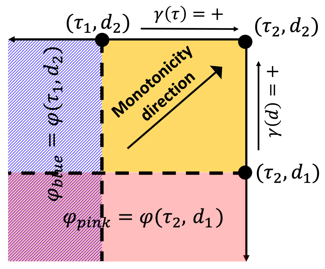
(a) $\varphi_{yellow}=\varphi(\tau_{2},d_{2})\wedge\neg\varphi_{pink}\wedge\neg\varphi_{blue}$.

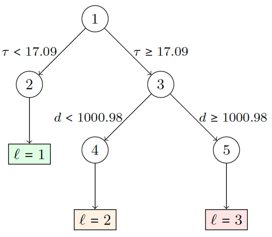
(b) The result of applying decision tree algorithm on labeled parameter valuations shown in Fig. 1a

Figure 3: Illustration of clustering on the BSS locations

Input: The learned projections $\pi$, labeling function $C$, threshold on the maximum depth of the Decision Tree $N$, parameter $K$ for k-fold cross validation method, threshold on the accuracy $ACC_{th}$

Output: The learned decision tree $DT$

// Loop over the maximum depth of Decision Tree

1 for $d\leftarrow 1$ to $N$ do

       // Compute the cross validation accuracy for $maxDepth=d$

2       $ACC_{d}=kfoldCrossValidation(\pi,C(\pi),maxDepth=d,K)$

       // Choose the max depth that gives the best cross validation accuracy

3       if $ACC_{d}>ACC_{th}$ then

             // Train a Decision Tree with the chosen max depth

4             $DT=fitDecisionTree(\pi,C(\pi),d)$

5             return $DT$

6            

7      

8return $\emptyset$;

9Function $kfoldCrossValidation(X,Y,maxDepth,K)$

       // Shuffle the data

10       $X,Y=Shuffle(X,Y)$

       // Devide the data into K subsets

11       $X(1:K),Y(1:K)=DivideToKSubsets(X,Y)$

12       $sumACC=0$

       // Train on K-1 subsets and test on 1 subset

13       for $i\leftarrow 1$ to $K$ do

14             $X_{train},Y_{train}=[X(1:i-1),X(i+1:K)],[Y(1:i-1),Y(i+1:K)]$

15             $X_{test},Y_{test}=X(i),Y(i)$

16             $DT=fitDecisionTree(X_{train},Y_{train},maxDepth)$

17             $ACC=predictDecisionTree(DT,X(i),Y(i))$

18             $sumACC=sumACC+ACC$

19            

      // Return the average accuracy

20       return $sumACC/K$

21      

Algorithm 3 K-fold cross validation approach to determine the best maximum depth of the Decision Tree

5 Case Studies

We now present the results of applying the clustering techniques developed on three benchmarks: (1) COVID-19 data from Los Angeles County, USA, (2) Outdoor Air Quality data from California, and (3) BSS data from the city of Edinburgh (running example). A summary of the computational aspects of the results is provided in Table. 2. The numbers indicate that our methods scale to spatial models containing hundreds of locations, and still learn interpretable STREL formulas for clusters.

Case	$|L|$	$|W|$	run-time (secs)	$\mathit{numC}$	$|\varphi_{\mathit{cluster}}|$
COVID-19	235	427	813.65	3	$3\cdot|\varphi|+4$
BSS	61	91	681.78	3	2 $\cdot|\varphi|+4$
Air Quality	107	60	136.02	8	$5\cdot|\varphi|+7$
Food Court*	20	35	78.24	8	$3\cdot|\varphi|+4$

Table 2: Summary of results.

COVID-19 data from LA County.  Understanding the spread pattern of COVID-19 in different areas is vital to stop the spread of the disease. While this example is not related to a software system, it is nevertheless a useful example to show the versatility of our approach to spatio-temporal data. The PSTREL formula $\varphi(c,d)=\diamonddiamond_{[0,d]}\{\mathbf{F}_{[0,\tau]}(x>c)$ allows us to number of cases exceeding a threshold $c$ within $\tau=10$ days in a neighborhood of size $d$ for a given location. Locations with small value of $d$ and large value of $c$ are unsafe as there is a large number of new positive cases within a small radius around them.

We illustrate the clustering results in Fig. 4. Each location in Fig. 4a is associated with a geographic region in LA county (shown in Fig. 4c), and the red cluster corresponds to hot spots (small $d$ and large $c$). Applying the DT classifier on the learned clusters (shown in Fig. 4a) produces 11 hyperboxes, some of which contain only a few points. Hence we apply our DT pruning procedure to obtain the largest cluster that gives us at least $90\%$ accuracy. Fig. 4b shows the results after pruning the Decision Tree. We learn the following formula:

$$\varphi_{red}=\diamonddiamond_{[0,4691.29]}(\mathbf{F}_{[0,10]}(x>3180))\vee\diamonddiamond_{[0,15000]}(\mathbf{F}_{[0,10]}(x>5611.5)),$$

This formula means that within 4691.29 meters from any red location, within 10 days, the number of new positive cases exceeds 3180. The COVID-19 data that we used is for September 2020.

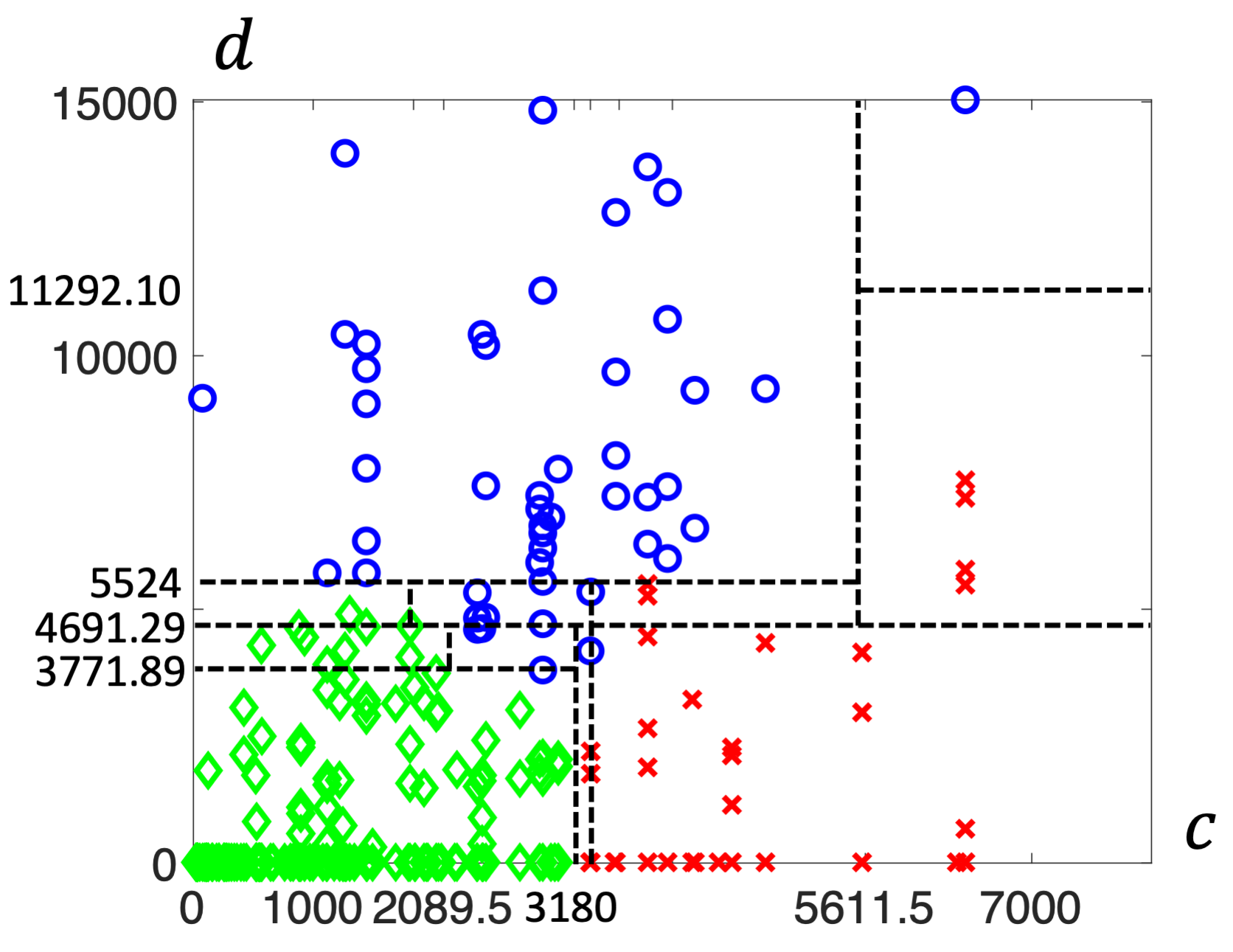
(a) The learned hyper-boxes before pruning the DT.

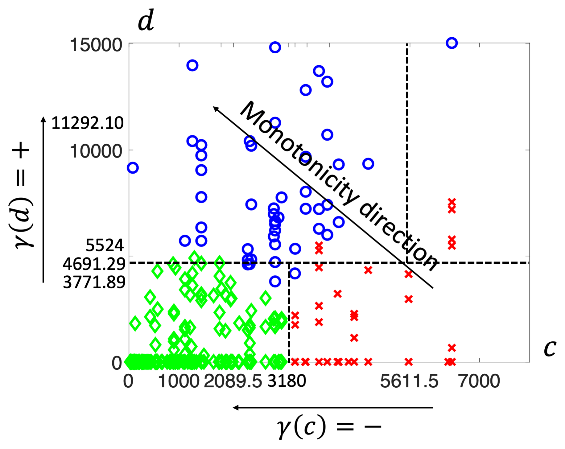
(b) The learned hyper-boxes after pruning the DT.

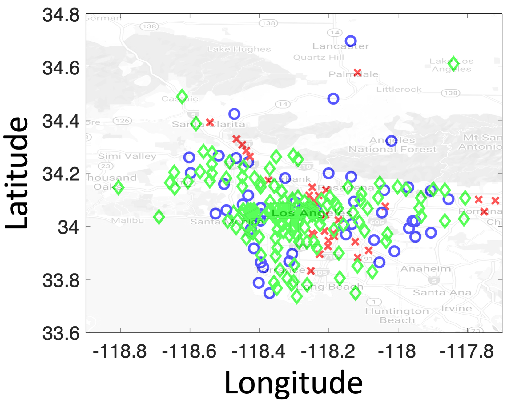
(c) Red-color points: hot spots.

Figure 4: Procedure to learn STREL formulas from COVID-19 data with template PSTREL formula $\varphi(c,d)=\diamonddiamond_{[0,d]}{}(\mathbf{F}_{[0,10]}(x>c))$

Outdoor Air Quality data from California.  We next consider Air Quality data from California gathered by the US Environmental Protection Agency (EPA). Among reported pollutants we focus on $PM2.5$ contaminant, and try to learn the patterns in the amount of $PM2.5$ in the air using STREL formulas. Consider a mobile sensing network consisting of UAVs to monitor pollution, such a STREL formula could be used to characterize locations that need increased monitoring.

We use the PSTREL formula $\varphi(c,d)$ = $\mathbf{G}_{[0,10]}(\mathcal{E}_{[d,16000]}{}(PM2.5<c))$ and project each location in California to the parameter space of $c,d$. A location $\ell$ satisfies this property if it is always true within the next 10 days, that there exists a location $\ell^{\prime}$ at a distance more than $d$, and a route $\tau$ starting from $\ell$ and reaching $\ell^{\prime}$ such that all the locations in the route satisfy the property $PM2.5<c$. Hence, it might be possible to escape to a location at a distance greater than $d$ always satisfying property $PM2.5<c$. The results are shown in Fig. 5a. Cluster 8 is the best cluster as it has a small value of $c$ and large value of $d$ which means that there exists a long route from the locations in cluster 8 with low density of $PM2.5$. Cluster 3 is the worst as it has a large value of $c$ and a small value of $d$. The formula for cluster $3$ is $\varphi_{3}$ = $\varphi(500,0)\wedge\neg\varphi(500,2500)\wedge\neg\varphi(216,0)$. $\varphi_{3}$ holds in locations where, in the next 10 days, $PM2.5$ is always less than $500$, but at least in 1 day $PM2.5$ reaches $216$ and there is no safe route (i.e. locations along the route have $PM2.5$ < 500) of length at least 2500.

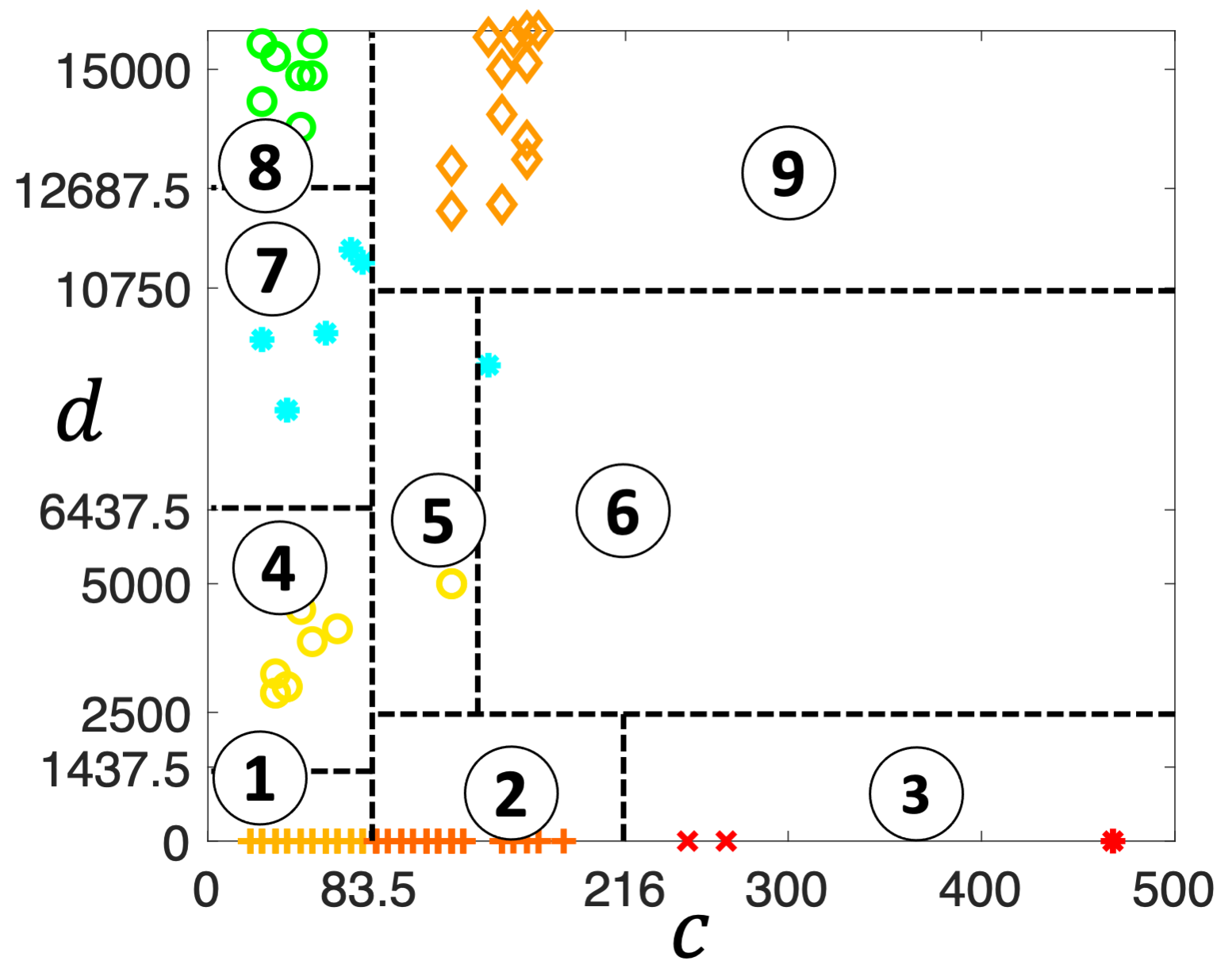
(a) The learned Hyper-boxes from Air Quality data.

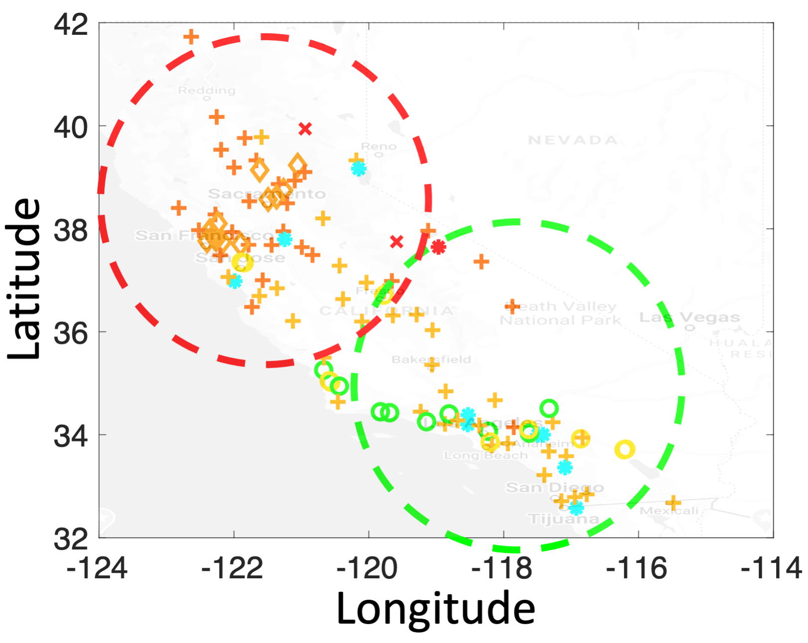
(b) Red and orange points: high density of $PM2.5$.

Figure 5: Clustering experiments on the California Air Quality Data

6 Related work and Conclusion

Traditional ML approaches for time-series clustering.  Time-series clustering is a popular area in the domain of machine learning and data mining. Some techniques for time-series clustering combine clustering methods such as KMeans, Hierarchical Clustering, agglomerative clustering and etc., with similarity metrics between time-series data such as the Euclidean distance, dynamic time-warping (DTW) distance, and statistical measures (such as mean, median, correlation, etc). Some recent works such as the works on shapelets automatically identify distinguishing shapes in the time-series data Zakaria et al. (2012). Such shapelets serve as features for ML tasks. All these approaches are based on shape-similarity which might be useful in some applications; however, for applications that the user is interested in mining temporal information from data, dissimilar traces might be clustered in the same group M. Vazquez-Chanlatte et al. (2017). Furthermore, such approaches may lack interpretablility as we showed in BSS case study.

STL-based clustering of time-series data.  There is considerable amount of recent work on learning temporal logic formulas from time-series data using logics such as Signal Temporal Logic (STL) M. Vazquez-Chanlatte et al. (2017); Jin et al. (2015); Mohammadinejad et al. (2020a, b); however, there is no work on discovering such relations on spatio-temporal data. In particular, the work in M. Vazquez-Chanlatte et al. (2017) which addresses unsupervised clustering of time-series data using Signal Temporal Logic is closest to our work. There are a few hurdles in applying such an approach to spatio-temporal data as explained in Section. LABEL:sec:intro. We address all the hurdles in the current work.

Monitoring spatio-temporal properties.  There is considerable amount of recent work such as Bartocci et al. (2017, 2020) on monitoring spatio-temporal properties. Particularly, MoonLight Bartocci et al. (2020) is a recent tool for monitoring of STREL properties, and in our current work, we use MoonLight for computing the robustness of spatio-temporal data with respect to STREL formulas. MoonLight uses $(\delta,d)$-connectivity approach for creating a spatial model, which has several issues, including dis-connectivity and distance overestimation. We resolve these issues by proposing our new method for creating the spatial graph, which we call Enhanced MSG. While there are many works on monitoring of spatio-temporal logic, to the best of our knowledge, there is no work on automatically inferring spatio-temporal logic formulas from data that we address in this work.

Conclusion.  In this work, we proposed a technique to learn interpretable STREL formulas from spatio-temporal time-series data for Spatially Distributed Systems. First, we introduced the notion of monotonicity for a PSTREL formula, proving the monotonicity of each spatial operator. We proposed a new method for creating a spatial model with a restrict number of edges that preserves connectivity of the spatial model. We leveraged quantitative semantics of STREL combined with multi-dimensional bisection search to extract features for spatio-temporal time-series clustering. We applied Agglomerative Hierarchical clustering on the extracted features followed by a Decision Tree based approach to learn an interpretable STREL formula for each cluster. We then illustrated with a number of benchmarks how this technique could be used and the kinds of insights it can develop. The results show that while our method performs slower than traditional ML approaches, it is more interpretable and provides a better insight into the data. For future work, we will study extensions of this approach to supervised and active learning.

Acknowledgments.  We thank the anonymous reviewers for their comments. The authors also gratefully acknowledge the support by the National Science Foundation under the Career Award SHF-2048094 and the NSF FMitF award CCF-1837131, and a grant from Toyota R&D North America.

Appendix

Appendix A Boolean and Quantitative Semantics of STREL

STREL is equipped with both Boolean and quantitative semantics; a Boolean semantics, $(\mathcal{S},\sigma,\ell,t)\models\varphi$, with the meaning that the spatio-temporal trace $\sigma$ in location $\ell$ at time $t$ with spatial model $\mathcal{S}$, satisfies the formula $\varphi$ and a quantitative semantics, $\rho(\varphi,\mathcal{S},\sigma,t)$, that can be used to measure the quantitative level of satisfaction of a formula for a given trajectory and space model. The function $\rho$ is also called the robustness function. The satisfaction of the whole trajectory correspond to the satisfaction at time $0$, i.e. $\rho(\varphi,\mathcal{S},\sigma)=\rho(\varphi,\mathcal{S},\sigma,0)$. Semantics for Boolean and temporal operator remain the same as STL Maler and Nickovic [2004]. We describe below the quantitative semantics of the spatial operators. Boolean semantics can be derived substituting $\min,\max$ with $\vee,\wedge$ and considering the Boolean satisfaction instead of $\rho$.

Reach

The quantitative semantics of the reach operator is:

$$\rho(\varphi_{1}\>\mathcal{R}_{[d_{1},d_{2}]}{}\>\varphi_{2},\mathcal{S},\sigma,\ell,t)=\max_{\tau\in\mathcal{T}(\mathcal{S},\ell)}\max_{\ell^{\prime}\in\tau:\left(d_{\mathcal{S}}^{\tau}(\ell^{\prime})\in[d_{1},d_{2}]\right)}\linebreak(\min(\rho(\varphi_{2},\mathcal{S},\sigma,\ell^{\prime},t),$$

$$\min_{j<\tau(\ell^{\prime})}\rho(\varphi_{1},\mathcal{S},\sigma,\tau[j],t)))$$

$(\mathcal{S},\sigma,\ell,t)$, a spatio-temporal trace $\sigma$, in location $\ell$, at time $t$, with a spatial model $\mathcal{S}$, satisfies $\varphi_{1}\>\mathcal{R}_{[d_{1},d_{2}]}{}\>\varphi_{2}$ iff it satisfies $\varphi_{2}$ in a location $\ell^{\prime}$ reachable from $\ell$ through a route $\tau$, with a length $d_{\mathcal{S}}^{\tau}(\ell^{\prime})\in[d_{1},d_{2}]$, and such that $\tau[0]=\ell$ and all its elements with index less than $\tau(\ell^{\prime})$ satisfy $\varphi_{1}$. Intuitively, the reachability operator $\varphi_{1}\mathcal{R}_{[d_{1},d_{2}]}{}\varphi_{2}$ describes the behavior of reaching a location satisfying property $\varphi_{2}$ passing only through locations that satisfy $\varphi_{1}$, and such that the distance from the initial location and the final one belongs to the interval $[d_{1},d_{2}]$.

Escape

The quantitative semantics of the escape operator is:

$$\rho(\mathcal{E}_{[d_{1},d_{2}]}{}\>\varphi,\mathcal{S},\sigma,\ell,t)=\max_{\tau\in\mathcal{T}(\mathcal{S},\ell)}\max_{\ell^{\prime}\in\tau:\left(d_{\mathcal{S}}^{\tau}[\ell,\ell^{\prime}]\in[d_{1},d_{2}]\right)}\linebreak~{}\min_{i\leq\tau(\ell^{\prime})}\rho(\varphi,\mathcal{S},\sigma,\tau[i],t).$$

$(\mathcal{S},\sigma,\ell,t)$, a spatio-temporal trace $\sigma$, in location $\ell$, at time $t$, with a spatial model $\mathcal{S}$, satisfies $\mathcal{E}_{[d_{1},d_{2}]}{}\>\varphi$ if and only if there exists a route $\tau$ and a location $\ell^{\prime}\in\tau$ such that $\tau[0]=\ell$, $d_{\mathcal{S}}^{\tau}[\tau[0],\ell^{\prime}]\in[d_{1},d_{2}]$ and all elements $\tau[0],...\tau[k]$ (with $\tau(\ell^{\prime})=k$) satisfy $\varphi$. Practically, the escape operator $\mathcal{E}_{[d_{1},d_{2}]}{}\varphi$, instead, describes the possibility of escaping from a certain region passing only through locations that satisfy $\varphi$, via a route with a distance that belongs to the interval $[d_{1},d_{2}]$.

Somewhere

$\diamonddiamond_{[d_{1},d_{2}]}{}\varphi:=true\mathcal{R}_{[d_{1},d_{2}]}{}\varphi$ holds for $(\mathcal{S},\sigma,\ell,t)$ iff there exists a location $\ell^{\prime}$ in $\mathcal{S}$ such that $(\mathcal{S},\sigma,\ell^{\prime},t)$ satisfies $\varphi$ and $\ell^{\prime}$ is reachable from $\ell$ via a route $\tau$ with length $d_{\mathcal{S}}^{\tau}[\ell^{\prime}]\in[d_{1},d_{2}]$.

Everywhere.

$\boxbox_{[d_{1},d_{2}]}{}\varphi:=\neg\diamonddiamond_{[d_{1},d_{2}]}{}\neg\varphi$ holds for $(\mathcal{S},\sigma,\ell,t)$ iff all the locations $\ell^{\prime}$ reachable from $\ell$ via a path,with length $d_{\mathcal{S}}^{\tau}[\ell^{\prime}]\in[d_{1},d_{2}]$, satisfy $\varphi$.

Surround

$\varphi_{1}\circledcirc_{[d_{1},d_{2}]}{}\varphi_{2}:=\varphi_{1}\wedge\neg(\varphi_{1}\mathcal{R}_{[d_{1},d_{2}]}{}\neg(\varphi_{1}\vee\varphi_{2}))\wedge\neg(\mathcal{E}_{[d_{2},\infty]}{}(\varphi_{1}))$ holds for $(\mathcal{S},\sigma,\ell,t)$ iff there exists a $\varphi_{1}$-region that contains $\ell$, all locations in that region satisfies $\varphi_{1}$ and are reachable from $\ell$ through a path with length less than $d_{2}$. Furthermore, all the locations that do not belong to the $\varphi_{1}$-region but are directly connected to a location in $\varphi_{1}$-region must satisfy $\varphi_{2}$ and be reached from $\ell$ via a path with length in the interval $[d_{1},d_{2}]$. Intuitively, the surround operator indicates the notion of being surrounded by a $\varphi_{2}$-region, while being in a $\varphi_{1}$-region, with some added constraints. The idea is that one cannot escape from a $\varphi_{1}$-region without passing from a node that satisfies $\varphi_{2}$ and, in any case, one has to reach a $\varphi_{2}$-node at a distance between $d_{1}$ and $d_{2}$.

Lemma 2

Let $\langle L,W\rangle$ be a spatial model where ${d_{\mathcal{S}}}_{\mathrm{min}}$ is the minimum distance between two locations and let $H_{[d_{1},d_{2}]}$ be a STREL formula where $H$ is an arbitrary spatial operator. Then, the complexity of monitoring formula is $O(k^{2}\cdot|L|\cdot|W|)$, where $k=\min\{i|i\cdot{d_{\mathcal{S}}}_{\mathrm{min}}>d_{2}\}$.

Appendix B Monotonicity Proofs for spatial operators

Lemma 3

The polarity for PSTREL formulas $\varphi(d_{1},d_{2})$ of the form $\psi_{1}\mathcal{R}_{[d_{1},d_{2}]}\psi_{2}$, $\mathcal{E}_{[d_{1},d_{2}]}\psi$, $\diamonddiamond_{[d_{1},d_{2}]}\psi$ and $\psi_{1}\circledcirc_{[d_{1},d_{2}]}\psi_{2}$ are $\gamma(d_{1})=-$ and $\gamma(d_{2})=+$, i.e. if a spatio-temporal trace satisfies $\varphi(\nu(d_{1}),\nu(d_{2}))$, then it also satisfies any STREL formula over a strictly larger spatial model induced distance interval, i.e. by decreasing $\nu(d_{1})$ and increasing $\nu(d_{2})$. For a formula $\boxbox_{[d_{1},d_{2}]}\psi$, $\gamma(d_{1})=+$ and $\gamma(d_{2})=-$, i.e. the formula obtained by strictly shrinking the distance interval.

Proof 2

To prove the above lemma, we first define some ordering on intervals. For intervals $I=[a,b]$ and $I^{\prime}=[a^{\prime},b^{\prime}]$,

$$I^{\prime}\geq I\iff a^{\prime}\leq a\;and\;b^{\prime}\geq b.$$

Followed by the defined ordering on intervals,

$$\max_{I^{\prime}}f(x)\geq\max_{I}f(x)\iff I^{\prime}\geq I$$ (2)

$$\min_{I^{\prime}}f(x)\leq\min_{I}f(x)\iff I^{\prime}\geq I$$ (3)

Assuming $d_{1}^{\prime}\leq d_{1}$ and $d_{2}^{\prime}\geq d_{2}$, from quantitative semantics of the Reach operator and equation. 2 we get:

$$\rho(\varphi_{1}\>\mathcal{R}_{[d_{1}^{\prime},d_{2}]}{}\>\varphi_{2},\mathcal{S},\sigma,\ell,t)\geq\rho(\varphi_{1}\>\mathcal{R}_{[d_{1},d_{2}]}{}\>\varphi_{2},\mathcal{S},\sigma,\ell,t),$$

$$\rho(\varphi_{1}\>\mathcal{R}_{[d_{1},d_{2}^{\prime}]}{}\>\varphi_{2},\mathcal{S},\sigma,\ell,t)\geq\rho(\varphi_{1}\>\mathcal{R}_{[d_{1},d_{2}]}{}\>\varphi_{2},\mathcal{S},\sigma,\ell,t),$$

which proves that the Reach operator is monotonically decreasing with respect to $d_{1}$ and monotonically increasing with respect to $d_{2}$. The proofs for other spatial operators are similar, and we skip for brevity.

Appendix C Case studies

C.1 COVID-19 data from LA County

COVID-19 pandemic has affected everyone’s life tremendously. Understanding the spread pattern of COVID-19 in different areas can help people to choose their daily communications appropriately which helps in decreasing the spread of the virus. Particularly, we consider COVID-19 data from LA County Kiamari et al. [2020] and use STREL formulas to understand the underlying patterns in the data. The data consists of the number of daily new cases of COVID-19 in different regions of LA County. In our analysis, we exclude the regions with more than $15\%$ missing values resulting in a total of 235 regions. For the remaining 235 regions, we fill the missing values with the nearest non-missing value. We construct the spatial model using our $(\alpha,d_{\mathrm{hvrsn}})$-Enhanced MSG approach with $\alpha=2$ which results in a total of 427 edges in the spatio-temporal graph. One of the important properties for a region is: “at some place within the radius of $d$ from the region, eventually within $\tau$ days, the number of new COVID-19 cases goes beyond a certain threshold c”. For simplicity, we fix $\tau$ to $10$ days, and we are interested in learning the tight values of $c$ and $d$ for each region in LA County. Regions with small value of $d$ and large value of $c$ are unsafe regions because there is a large number of new positive cases within a small radius around such regions. However, regions with large values of $d$ and small values of $c$ are potentially safe regions because within a large radius around such regions there is only a small number of new positive cases. This property can be specified using PSTREL formula $\varphi(c,d)=\diamonddiamond_{[0,d]}{}\{\mathbf{F}_{[0,\tau]}(x>c)$. To learn the tight values of $c$ and $d$ for each region in LA County we use the lexicographic projection approach formalized in Algo. 2 (assuming that $\tau$ is fixed to 10 days and ordering of $c>_{\mathcal{P}}d$ on parameters). This technique projects each region in LA county to a representative point in the parameter space of $\varphi$. Next, we use Agglomerative Hierarchical Clustering to cluster the regions into multiple groups with respect to $\varphi$. We use the learned parameter valuations $(c,d)$ as features for clustering algorithm with the number of clusters as $k=3$. The results are illustrated in Fig. 4.

The red cluster consists of the unsafe region or hot spots since it has small $d$ and large $c$. Each point in Fig. 4a is associated with a region in LA County illustrated in Fig. 4c. The total time for learning the clusters from spatio-temporal data is 813.65 seconds. Next, we are interested in learning an interpretable STREL formula for each cluster using our Decision Tree based approach. The result of applying the Decision Tree classifier on the learned clusters is shown as dash-lines in Fig. 4a. To do a perfect separation, the Decision Tree learns 11 hyper-boxes which some of them only contain a negligible number of data points. While using all the 11 hyper-boxes results in guaranteed STREL formulas for each cluster of points, the STREL formulas that are learned might be complicated and hence not interpretable. To mitigate this issue and improve the interpretability of the learned STREL formulas for each cluster, we try to learn an approximate STREL formula for each cluster of points using the Decision Tree pruning method proposed in Algo. 3.

We compute an STREL formula for each cluster as follows:

$$\varphi_{blue}=\varphi(0,15000)\wedge\neg\varphi(0,4691.29)\wedge\neg\varphi(5611.5,15000)=\neg\varphi(0,4691.29)\wedge$$

$$\neg\varphi(5611.5,15000)$$

$$\varphi_{green}=\varphi(0,4691.29)\wedge\neg\varphi(0,0)\wedge\neg\varphi(3180,4691.29)=\varphi(0,4691.29)\wedge$$

$$\neg\varphi(3180,4691.29)$$

$$\varphi^{1}_{red}=\varphi(3180,4691.29)\wedge\neg\varphi(8000,4691.29)\wedge\neg\varphi(3180,0)=\varphi(3180,4691.29)$$

$$\varphi^{2}_{red}=\varphi(5611.5,15000)\wedge\neg\varphi(8000,15000)\wedge\neg\varphi(5611.5,4691.29)=$$

$$\varphi(5611.5,15000)$$

$$\varphi{red}=\varphi^{1}_{red}\vee\varphi^{2}_{red}.$$

By replacing $\varphi(c,d)$ with $\diamonddiamond_{[0,d]}{}\{\mathbf{F}_{[0,10]}(x>c)\}$ in the above STREL formulas we get:

$$\varphi_{blue}=\boxbox_{[0,4691.29]}{}\{G_{[0,10]}(x=0)\}\wedge\boxbox_{[0,15000]}{}\{G_{[0,10]}(x<5611.5)\}$$

$$\varphi_{green}=\diamonddiamond_{[0,4691.29]}{}\{\mathbf{F}_{[0,10]}(x>0)\}\wedge\boxbox_{[0,4691.29]}{}\{G_{[0,10]}(x<3180)\}$$

$$\varphi^{1}_{red}=\diamonddiamond_{[0,4691.29]}{}\{\mathbf{F}_{[0,10]}(x>3180)\}$$

$$\varphi^{2}_{red}=\diamonddiamond_{[0,15000]}{}\{\mathbf{F}_{[0,10]}(x>5611.5)\}$$

$$\varphi_{red}=\varphi^{1}_{red}\vee\varphi^{2}_{red}=\diamonddiamond_{[0,4691.29]}{}\{\mathbf{F}_{[0,10]}(x>3180)\}\vee$$

$$\diamonddiamond_{[0,15000]}{}\{\mathbf{F}_{[0,10]}(x>5611.5)\}$$

The learned formula for the blue cluster is $\varphi_{blue}=\boxbox_{[0,4691.29]}{}\{G_{[0,10]}(x=0)\}\wedge\boxbox_{[0,15000]}{}\{G_{[0,10]}(x<5611.5)\}$, which means that within the radius of 4691.29 meters around the blue points, in the next 10 days, there is no new positive cases. By increasing the radius to 15000 meters there is new positive cases but the number does not exceed 5611. The learned formula for the green cluster is $\varphi_{green}=\diamonddiamond_{[0,4691.29]}{}\{\mathbf{F}_{[0,10]}(x>0)\}\wedge\boxbox_{[0,4691.29]}{}\{G_{[0,10]}(x<3180)\}$, which means that within the radius of 4691.29 meters from the green points, at some point in the next 10 days, there will be new positive cases but the number will not exceed 3180. Finally, formula $\varphi_{red}=\diamonddiamond_{[0,4691.29]}{}\{\mathbf{F}_{[0,10]}(x>3180)\}\vee\diamonddiamond_{[0,15000]}{}\{\mathbf{F}_{[0,10]}(x>5611.5)\}$ which is learned for the red cluster means that within the radius of 4691.29 meters from the red points, in the next 10 days, the number of new positive cases exceeds 3180. By increasing the radius to 15000, in some region within this radius, the number of new positive cases goes beyond 5611. Thus, the regions associated with the red points (illustrated in Fig. 4c) are the hot spots and people should avoid any unnecessary communications in these regions in the next 10 days. The COVID-19 data that we considered is for September 2020. In Fig. 6, we show the results of clustering for 3 different months in 2020, which confirms the rapid spread of the COVID-19 virus in LA county from April 2020 to September 2020.

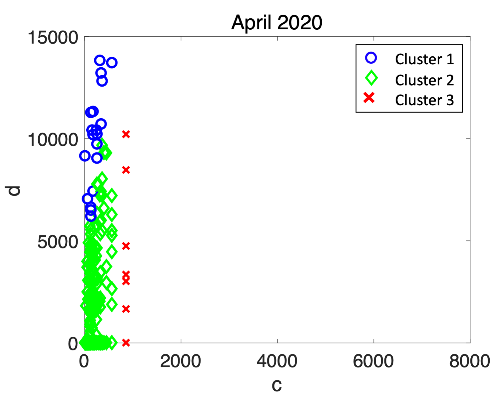
(a) Clusters learned from the COVID-19 data for April 2020.

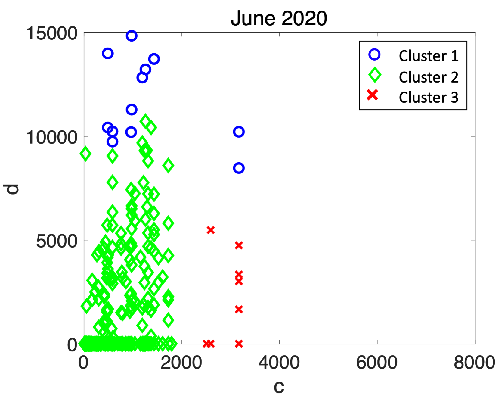
(b) Clusters learned from the COVID-19 data for June 2020.

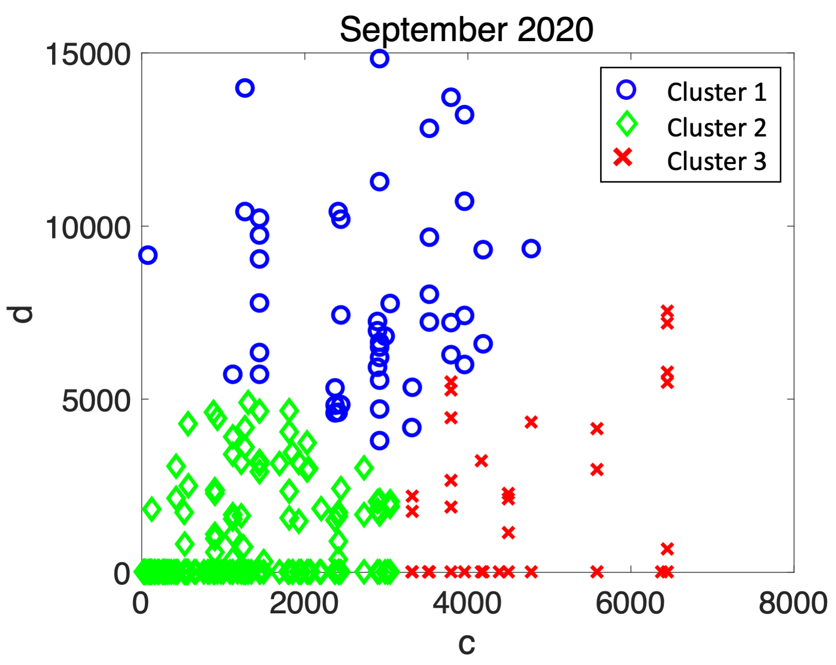
(c) Clusters learned from the COVID-19 data for September 2020.

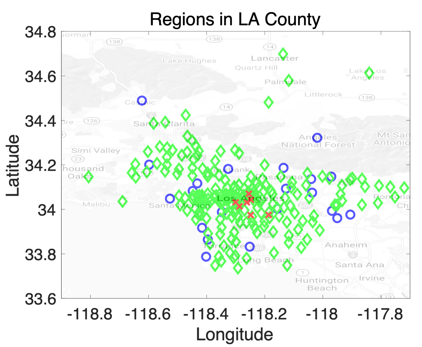
(d) Regions in LA county associated with the learned clusters from the COVID-19 data for April 2020.

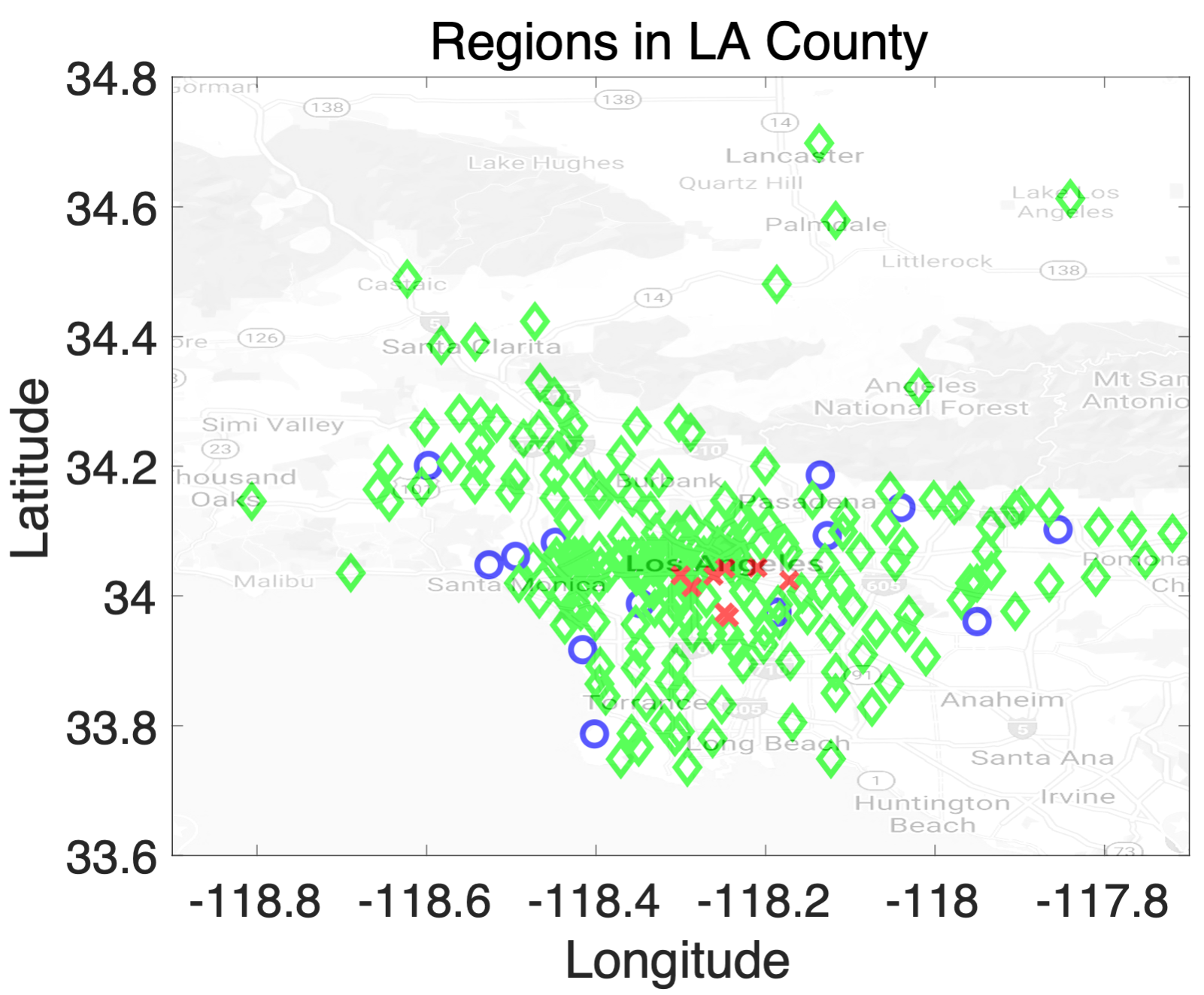
(e) Regions in LA county associated with the learned clusters from the COVID-19 data for June 2020.

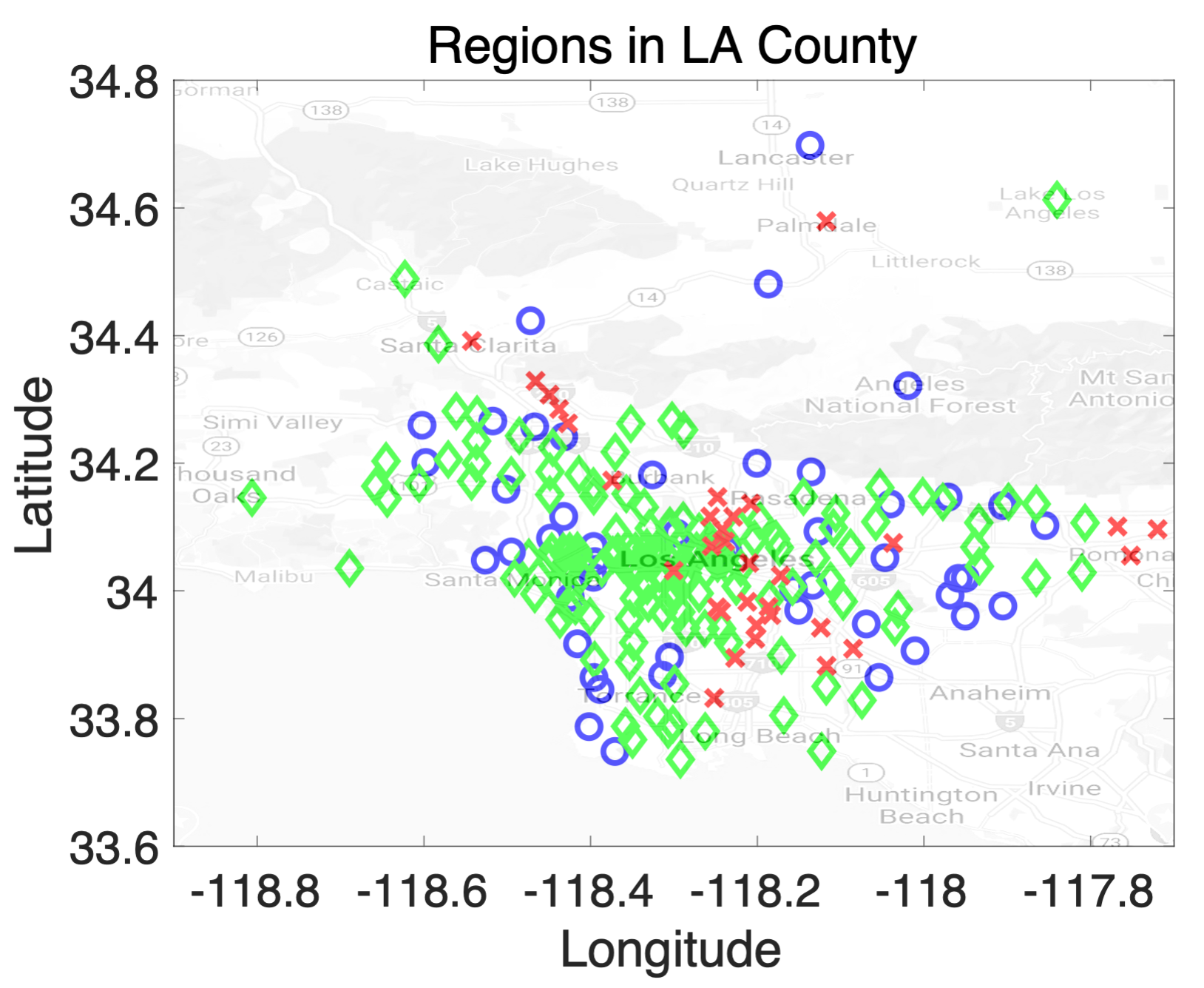
(f) Regions in LA county associated with the learned clusters from the COVID-19 data for September 2020.

Figure 6: Changing of clustering with respect to time for the COVID-19 data and PSTREL formula $\varphi(c,d)$ with $\diamonddiamond_{[0,d]}{}\{\mathbf{F}_{[0,10]}(x>c)\}$. The plots confirm the rapid spread of the COVID-19 virus in LA county from April 2020 to September 2020.

C.2 BSS data from the city of Edinburgh

Bike-Sharing System is an affordable and popular form of transportation that has been introduced to many cities such as the city of Edinburgh in recent years Kreikemeyer et al. [2020]. Each BSS consists of a number of bike stations, distributed over a geographic area, and each station has a fixed number of bike slots. The users can pick up a bike, use it for a while, and then return it to the same or another station in the area. It is important for a BSS to satisfy the demand of its users. For example, “within a short time, there should always be a bike and empty slot available in each station or its adjacent stations”. Otherwise, the user either has to wait a long time in the station or walk a long way to another far away station that has bike/slot availability. Understanding the behavior of a BSS can help users to decide on which station to use and also help operators to choose the optimal number of bikes/empty slots for each station. In this work we use STREL formulas to understand the behavior of BSS. Particularly, we consider the BSS in the city of Edinburgh which consist of 61 stations (excluding the stations with more than $15\%$ missing value). We construct the spatial model using the $(\alpha,d_{\mathrm{hvrsn}})$-Enhanced MSG approach with $\alpha=2$ resulting in a total of 91 edges in the spatial model. A BSS should have at least one of two important properties to satisfy the demand of users. The first property is: “a bike/empty slot should be available in the station within a short amount of time”. The second property is “if there is no bike/empty slot available in a station, there should be a bike/empty slot available in the nearby stations”. The first property can be described using PSTREL formula $\varphi_{wait}(\tau)=(\mathbf{F}_{[0,\tau]}Bikes\geq 1)\wedge(\mathbf{F}_{[0,\tau]}Slots\geq 1)$, which means that at some time within the next $\tau$ seconds, there will be at least one bike/empty slot available in the station. Stations with small values of $\tau$ have short wait time which is desirable for the users, and stations with large values of $\tau$ have long wait times which is undesirable. For the second case, the users might prefer to walk a short distance to nearby stations instead of waiting a long time in the current station for a bike/slot to be available; this is related to the second important property of a BSS. The associated PSTREL formula for the second property is $\varphi_{walk}(d)=(\diamonddiamond_{[0,d]}{}Bikes\geq 1)\wedge(\diamonddiamond_{[0,d]}{}Slots\geq 1)$, which means that “at some station within the radius d of the current station, there is at least one bike/empty slot available”. If the value of $d$ for a station is large, this means that the user should walk a long way to far stations to find a bike/empty slot available. We combine the two PSTREL formulas into $\varphi(\tau,d)=G_{[0,3]}\{\varphi_{wait}(\tau)\vee\varphi_{walk}(d)\}$, which means that always within the next 3 hours at least one of the properties $\varphi_{wait}(\tau)$ or $\varphi_{walk}(d)$ should hold. We try to learn the tight value of $\tau$ and $d$ for each station. Stations with small values of $\tau$ and $d$ are desirable stations. We first apply Algo. 2 with the order $d>_{\mathcal{P}}\tau$ to learn the tight parameter valuations, and then apply our clustering followed by a Decision Tree algorithm to learn separating hyper-boxes for the clusters. The results are illustrated in Fig. 1a.

Green points that have small values of $\tau$ and $d$ are desirable stations. The orange point is associated with a station with a long wait time (around $35$ minutes). The red points are the most undesirable stations as they have a long wait time and do not have nearby stations that have bike/empty slots availability. Fig. 1b shows the location of each station on map which confirms that the stations associated with the red points are far from other stations. That’s the reason for having a large value of $d$. The time that takes to learn the clusters is 681.78 seconds. Next, we try to learn an interpretable STREL formula for each cluster based on the monotonicity direction of $\tau$ and $d$ as follows:

$$\varphi_{green}=\varphi(17.09,2100)\wedge\neg\varphi(0,2100)\wedge\neg\varphi(17.09,0)=\varphi(17.09,2100)$$

$$\varphi_{orange}=\varphi(50,1000.98)\wedge\neg\varphi(17.09,1000.98)\wedge\varphi(50,0)=\varphi(50,1000.98)\wedge$$

$$\neg\varphi(17.09,1000.98)$$

$$\varphi_{red}=\varphi(50,2100)\wedge\neg\varphi(17.09,2100)\wedge\neg\varphi(50,1000.98)=\neg\varphi(17.09,2100)\wedge$$

$$\neg\varphi(50,1000.98)$$

By replacing $\varphi(\tau,d)$ with $G_{[0,3]}\{\varphi_{wait}(\tau)\vee\varphi_{walk}(d)\}$ in the above STREL formulas we get:

$$\varphi_{green}=G_{[0,3]}\{\varphi_{wait}(17.09)\vee\varphi_{walk}(2100)\}$$

$$\varphi_{orange}=G_{[0,3]}\{\varphi_{wait}(50)\vee\varphi_{walk}(1000.98)\}\wedge$$

$$\neg G_{[0,3]}\{\varphi_{wait}(17.09)\vee\varphi_{walk}(1000.98)\}$$

$$\varphi_{red}=\neg G_{[0,3]}\{\varphi_{wait}(17.09)\vee\varphi_{walk}(2100)\}\wedge$$

$$\neg G_{[0,3]}\{\varphi_{wait}(50)\vee\varphi_{walk}(1000.98)\}$$

The intuition behind the learned STREL formula for the green cluster is that always within the next 3 hours the wait time for bike/slot availability is less than 17.09 minutes, or the walking distance to the nearby stations with bike/slot availability is less than 2100 meters. Fig. 1a illustrates that the actual walking distance for green points is less than or equal to 1000.98 meters, and the reason for learning 2100 meters is that the Decision Tree tries to learn robust and relaxed boundaries for each class. The STREL formula $\varphi_{orange}$ means that for the next 3 hours at least one of the properties $\varphi_{wait}(50)$ or $\varphi_{walk}(1000.98)$ holds for the orange stations. However, for a smaller wait time equal to 17.09 seconds, at least once in the next 3 hours, both the properties $\varphi_{wait}(17.09)$ and $\varphi_{walk}(1000.98)$ do not hold. The intuition behind the learned STREL formula for the orange stations is that, the orange stations have long wait time because they satisfy the property $G_{[0,3]}\{\varphi_{wait}(50)\vee\varphi_{walk}(1000.98)\}$ and falsify the property $G_{[0,3]}\{\varphi_{wait}(17.09)\vee\varphi_{walk}(1000.98)\}$. The red points falsify the property $G_{[0,3]}\{\varphi_{wait}(17.09)\vee\varphi_{walk}(2100)\}$ which is associated with a short wait time and the property $G_{[0,3]}\{\varphi_{wait}(50)\vee\varphi_{walk}(1000.98)\}$ which is associated with the short walking distance. Therefore, the red points are the most undesirable stations.

Comparison with Traditional ML approaches. To compare our framework with traditional ML approaches, we apply KMeans clustering from tslearn library Tavenard et al. [2020], which is a library in Python for analysis of time-series data, on the BSS data which uses DTW for similarity metric. The results of clustering are represented in Fig. 7. We also apply k-Shape clustering from tslearn library on the same dataset, where the results are illustrated in Fig. 8. k-Shape is a partitional clustering algorithm that preserves the shapes of time series. While KMeans and k-Shape clustering approaches perform faster than our approach (both approaches run in less than 5 seconds), the artifacts trained by these approaches often lack interpretability despite our approach (for example, identifying stations with long wait time or far away stations). Furthermore, since our learning approach for each node/location is independent of other locations, it is possible to improve the run-time by parallelization.

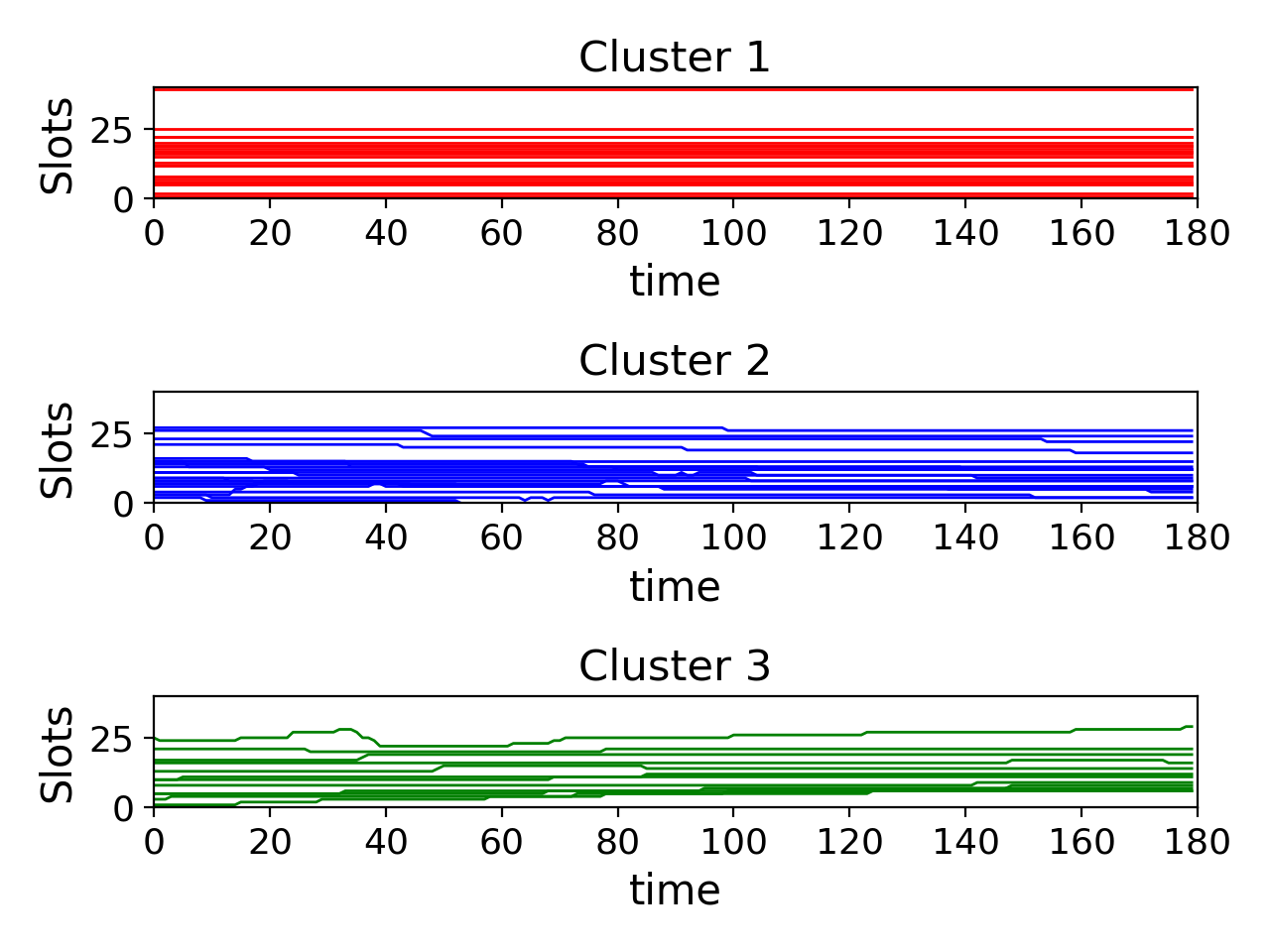
(a) Clusters learned from BSS data

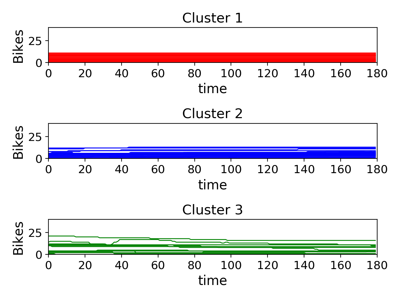
(b) Clusters learned from BSS data

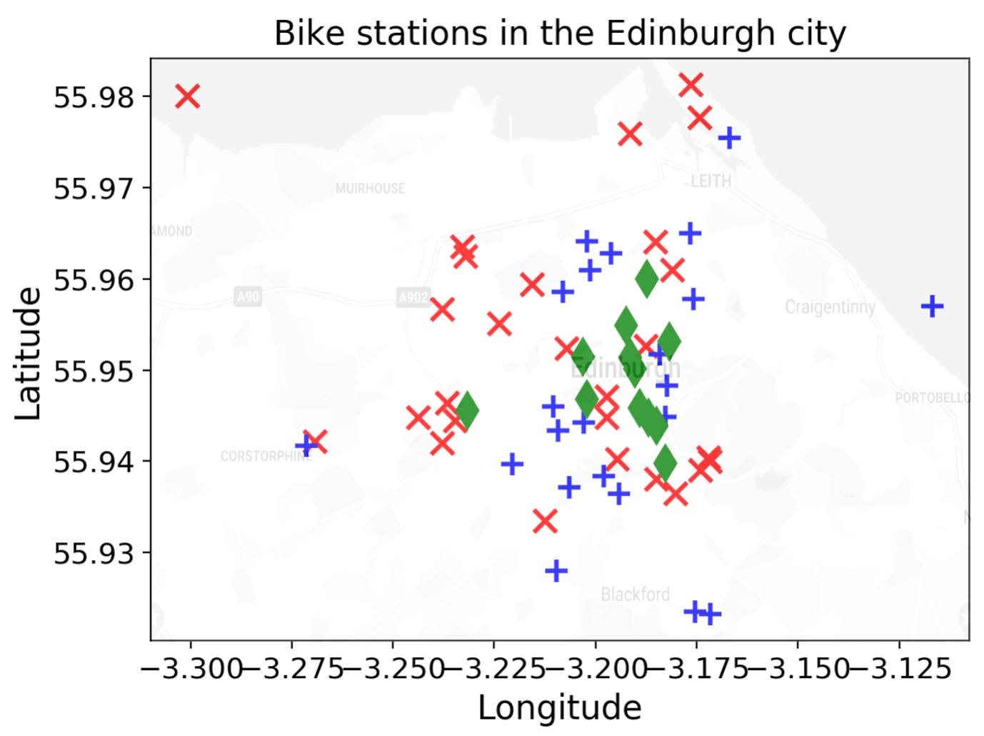
(c) Regions in Edinburgh city associated with the learned clusters.

Figure 7: Using KMeans approach from tslearn library with DTW metric to cluster BSS spatio-temporal traces.

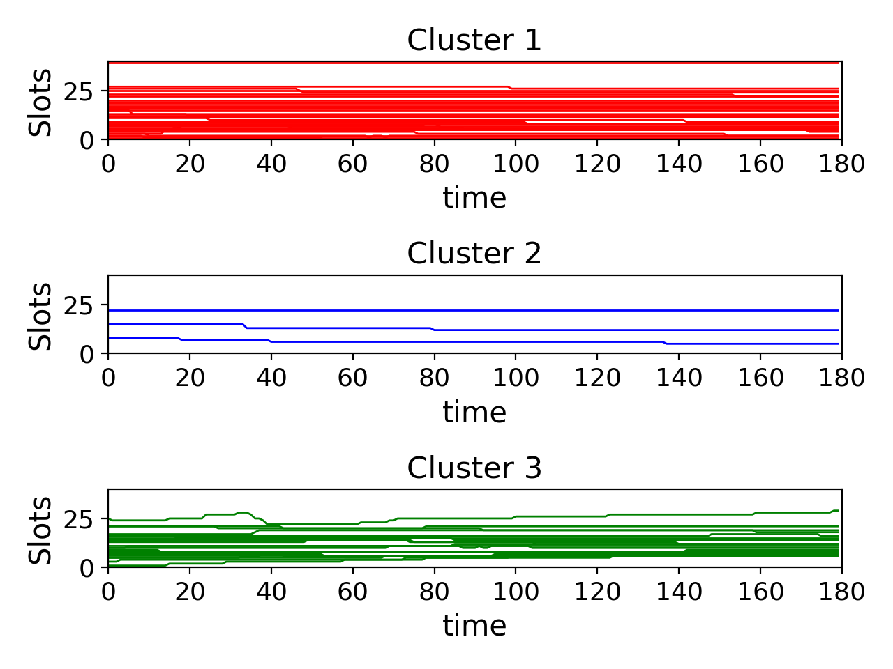
(a) Clusters learned from BSS data

(b) Clusters learned from BSS data

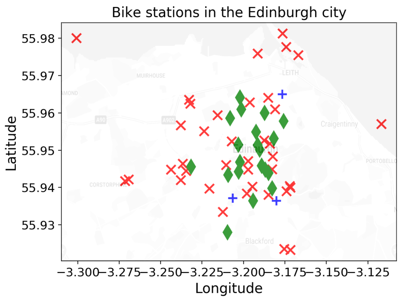
(c) Regions in Edinburgh city associated with the learned clusters.

Figure 8: Using Kshape approach from tslearn library to cluster BSS spatio-temporal traces.

C.3 Outdoor Air Quality data from California

Air pollution is one of the most important emerging concerns in environmental studies which can result in global warming and climate change. Most importantly, air pollution was ranked among the top leading cause of death in the world Gunawan et al. [2018]. For example, particulate matters smaller than $2.5\mu m$ (PM2.5) can deeply penetrate into lung and impair its functions Xing et al. [2016]. As a result, scientist are using the concentration of PM2.5 in air as the most important air quality index. Therefore, understanding the pattern of air pollutants like PM2.5 in different regions of a city is of significant importance because it can help people to take the necessary precautions such as preventing unnecessary communications in pollutant areas. In this work, we consider the Air Quality data from California that has been gathered by the United States Environmental Protection Agency (US EPA). Among reported pollutants we focus on PM2.5 contaminant, and try to learn the patterns in the amount of PM2.5 in the air using STREL formulas. The standard levels of PM2.5 are as follows: (1) $0\leq PM2.5\leq 12.0\mu g/m^{3}$ is considered as good, (2) $12.1\leq PM2.5\leq 35.4\mu g/m^{3}$: moderate, (3) $35.5\leq PM2.5\leq 55.4\mu g/m^{3}$: unhealthy for sensitive groups, and (4) $55.5\leq PM2.5$ is considered as unhealthy. To create the spatial model, we use the $(\alpha,d)$-Enhanced MSG Spatial Model approach with $\alpha=2$, resulting in a total of 160 edges. We consider the PSTREL formula $\varphi(c,d)=G_{[0,10]}\{\mathcal{E}_{[d,16000]}{}(PM2.5<c)\}$, and try to find the tight values of $c$ and $d$ for each region in California. A location $\ell$ will satisfy this property if it is always true within the next 10 days, that there exists a location $\ell^{\prime}$ at a distance more than $d$, and a route $\tau$ starting from $\ell$ and reaching $\ell^{\prime}$ such that all the locations in the route satisfy the property $PM2.5<c$. Hence, it might be possible to escape at a distance greater than $d$ always satisfying property $PM2.5<c$. The result of applying our learning method on Air Quality data with respect to this PSTREL formula is illustrated in Fig. 5a. The run-time of the algorithm is 136.02 seconds. Cluster 8 is the best cluster as it has a small value of $c$ and large value of $d$ which means that there exists a long route from the point in cluster 8 with low density of PM2.5. Cluster 3 is the worst cluster as it has a large value of $c$ and a small value of $d$, which means that the density of $PM2.5$ in these regions is extremely high. We try to learn an STREL formula for clusters 8 and 3 as follows:

$$\varphi_{3}=\varphi(500,0)\wedge\neg\varphi(500,2500)\wedge\neg\varphi(216,0)=G_{[0,10]}\{\mathcal{E}_{[0,16000]}{}(PM2.5<500)\}\wedge$$

$$\neg G_{[0,10]}\{\mathcal{E}_{[2500,16000]}{}(PM2.5<500)\}\wedge\neg G_{[0,10]}\{\mathcal{E}_{[0,16000]}{}(PM2.5<216)\}$$

$$\varphi_{8}=\varphi(83.5,12687.5)\wedge\neg\varphi(0,12687.5)\wedge\neg\varphi(83.5,15000)=\varphi(83.5,12687.5)=$$

$$G_{[0,10]}\{\mathcal{E}_{[12687.5,16000]}{}(PM2.5<83.5)\}$$

The formula $\varphi_{3}$ holds in locations where, in the next 10 days, $PM2.5$ is always less than $500$, but at least in 1 day $PM2.5$ reaches $216$ and at least in 1 day there is no safe paths reaching locations at the distance greater than 2500 where all the locations in the routes have still $PM2.5<500$. The formula $\varphi_{8}$ holds in all the locations where it is always true, within the next 10 days, that there exists a route reaching a location at a distance greater than 12687.5 m from the the current one, such that all the locations in the route have $PM2.5$ less than $83.5$

C.4 Food Court Building

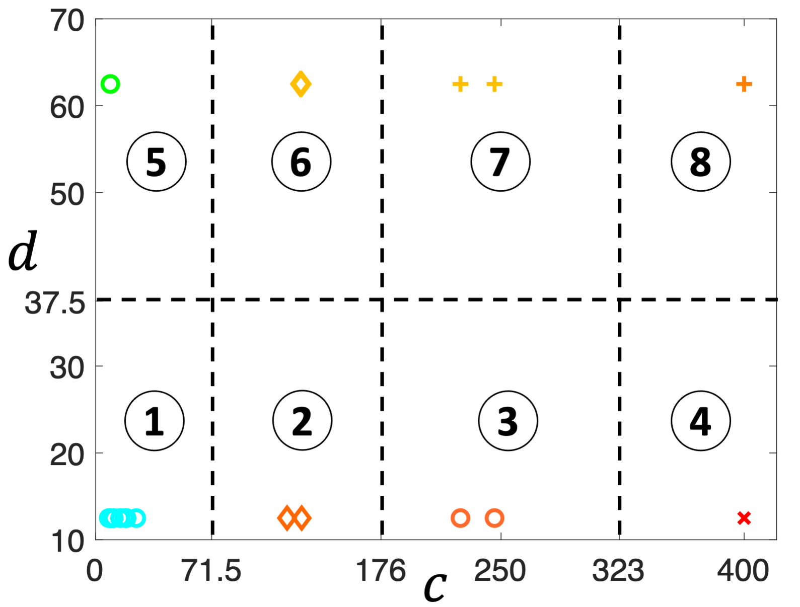
(a) Clusters learned from Food Court data.

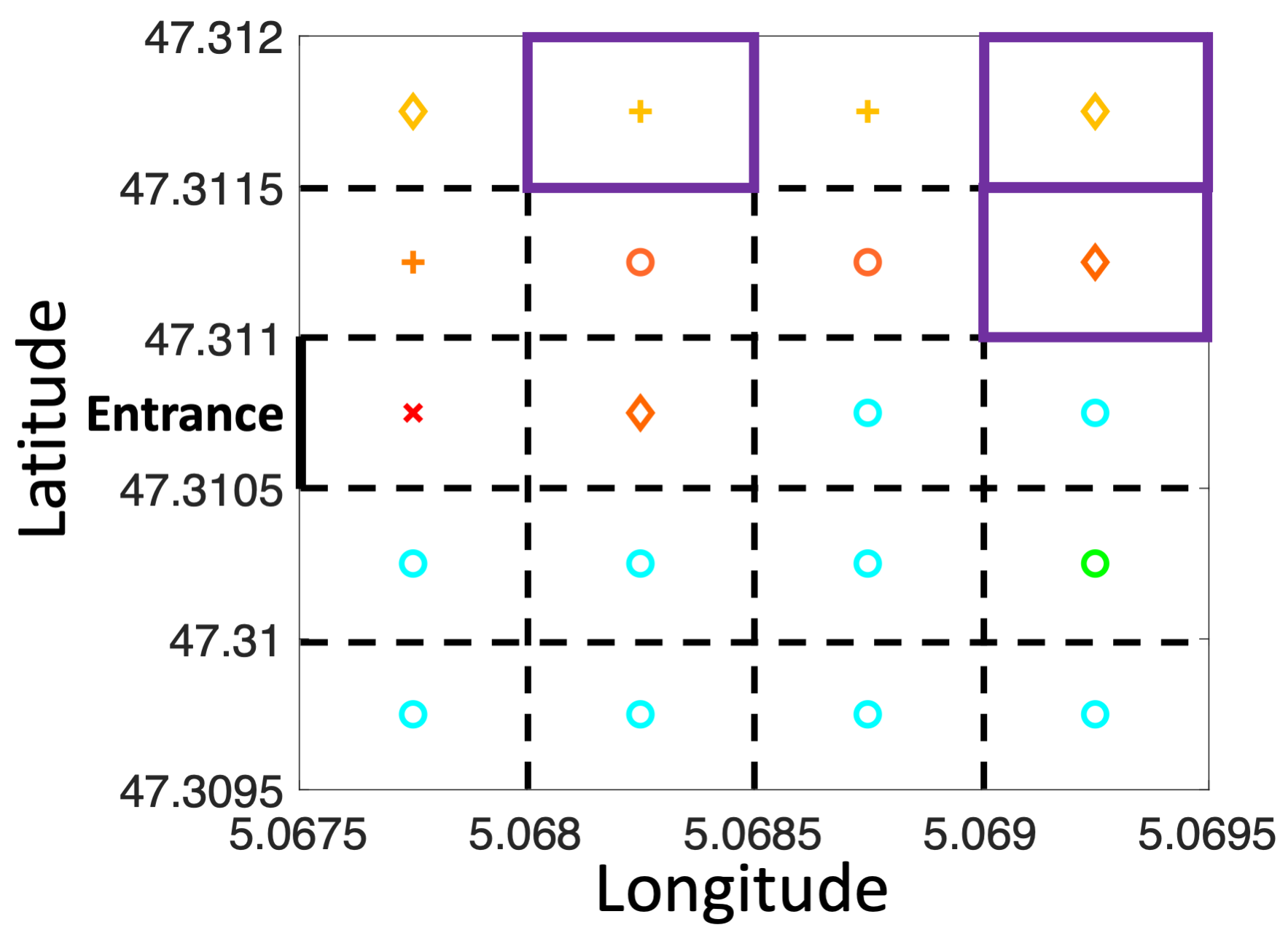
(b) Locations in the Food Court associated with the learned clusters.

Figure 9:

Here, we consider a synthetic dataset that simulates movements of customers in different areas of a food court. Due to COVID-19 pandemic, we are interested in identifying crowded areas in the food court, to help managers of the food court to have a better arrangement of different facilities (for example, keeping the popular restaurants in the food court separated) to prevent crowded area. To synthesize the dataset, we divide the food court into 20 regions, considering one of the regions as entrance, and three of them as popular restaurants. We create the dataset using the following steps: (1) we make a simplifying assumption that all of the customers enter the food court at time 0, which means that we set initial location of each customer as entrance (2) in every 10 minutes, we choose a random destination for each customer. The destination can be current location of the customer (in this case the customer does not go anywhere), one of the popular areas (we choose the probability as 0.8) or other areas of the food court. After choosing the destination for each customer, we simulate moving of the customer towards the destination with speed of $1.4m/s$, which is the average speed of walking. To create the spatial model, we assume the centers of each of the 20 regions as a node and connect the 20 nodes using the $(\alpha,d_{\mathrm{hvrsn}})$-Enhanced MSG approach with $\alpha=2$ resulting in 35 edges in the graph. The PSTREL formula $\varphi(c,d)=\diamonddiamond_{[0,d]}{}\{\mathbf{F}_{[0,3]}(numPeople>c)\}$ means that somewhere within the radius $d$ from a location, at least once in the next 3 hours, the number of people in the location exceeds the threshold $c$. Using this property, we can identify the crowded areas, and take necessary actions to mitigate the spread of COVID-19 in the Food Court area. We apply our method on the synthetic dataset that simulates the movements of customers in a Food Court, and try to learn the tight values of $d$ and $c$ for each location followed by clustering and our Decision Tree classification approach. The run-time of our learning approach is 78.24 seconds, and the results are illustrated in Fig. 9a. Cluster 4 which has a large value of $c$ and a small value of $d$ is associated with the most crowded area. We show the locations in the Food Court associated with each cluster in Fig. 9b. The results show a larger value of $c$ for the entrance and popular restaurants which confirm that these area are more crowded compared to other locations in the Food Court. Next, we try to learn an STREL formula for cluster 4 (associated with the most crowded location) and cluster 5 (associated with the most empty location) as follows:

$$\varphi_{4}=\varphi(323,37.5)\wedge\neg\varphi(323,10)\wedge\neg\varphi(420,37.5)=\varphi(323,37.5)=$$

$$\diamonddiamond_{[0,37.5]}{}\{\mathbf{F}_{[0,3]}(numPeople>323)\}$$

$$\varphi_{5}=\varphi(0,70)\wedge\neg\varphi(71.5,70)\wedge\neg\varphi(0,37.5)=\diamonddiamond_{[0,70]}{}\{\mathbf{F}_{[0,3]}(numPeople>0)\}\wedge$$

$$\boxbox_{[0,70]}{}\{G_{[0,3]}(numPeople\leq 71.5)\}\wedge\boxbox_{[0,37.5]}{}\{G_{[0,3]}(numPeople=0)\}$$

The STREL formula $\varphi_{4}$ means that somewhere within the radius 37.5 meters from the location, at least once within the next 3 hours, the number of people exceeds 323 which shows a crowded area. The learned formula for cluster 5 means that for the next 3 hours there will be no one in the radius 37.5 from the location. However, between the radius 37.5 and 70 from the location, there will be some people but the number does not exceed 72.

References

- Nenzi et al. [2018] Laura Nenzi, Luca Bortolussi, Vincenzo Ciancia, Michele Loreti, and Mieke Massink. Qualitative and quantitative monitoring of spatio-temporal properties with SSTL. LMCS, 14(4), 2018.
- Fiedler and Scheel [2003] Bernold Fiedler and Arnd Scheel. Spatio-temporal dynamics of reaction-diffusion patterns. Trends in nonlinear analysis, pages 23–152, 2003.
- Bartocci et al. [2017] Ezio Bartocci, Luca Bortolussi, Michele Loreti, and Laura Nenzi. Monitoring mobile and spatially distributed cyber-physical systems. In Proc. of MEMOCODE, 2017.
- Bartocci et al. [2020] Ezio Bartocci, Luca Bortolussi, Michele Loreti, Laura Nenzi, and Simone Silvetti. Moonlight: A lightweight tool for monitoring spatio-temporal properties. In Proc. of RV, 2020.
- M. Vazquez-Chanlatte et al. [2017] Marcell M. Vazquez-Chanlatte, J. V. Deshmukh, X. Jin, and S. A. Seshia. Logical clustering and learning for time-series data. In Proc. of CAV, 2017.
- Jin et al. [2015] Xiaoqing Jin, Alexandre Donzé, Jyotirmoy V Deshmukh, and Sanjit A Seshia. Mining requirements from closed-loop control models. IEEE Transactions on CAD, 34(11):1704–1717, 2015.
- Mohammadinejad et al. [2020a] Sara Mohammadinejad, Jyotirmoy V Deshmukh, Aniruddh G Puranic, Marcell Vazquez-Chanlatte, and Alexandre Donzé. Interpretable classification of time-series data using efficient enumerative techniques. In Proc. of HSCC, 2020a.
- Mohammadinejad et al. [2020b] Sara Mohammadinejad, Jyotirmoy V Deshmukh, and Aniruddh G Puranic. Mining environment assumptions for cyber-physical system models. In Proc. of ICCPS, 2020b.
- Maler and Nickovic [2004] Oded Maler and Dejan Nickovic. Monitoring temporal properties of continuous signals. In Formal Techniques, Modelling and Analysis of Timed and Fault-Tolerant Systems, pages 152–166. Springer, 2004.
- Asarin et al. [2011] Eugene Asarin, Alexandre Donzé, Oded Maler, and Dejan Nickovic. Parametric identification of temporal properties. In Proc. of RV, 2011.
- Vazquez-Chanlatte et al. [2018] Marcell Vazquez-Chanlatte, Shromona Ghosh, Jyotirmoy V Deshmukh, Alberto Sangiovanni-Vincentelli, and Sanjit A Seshia. Time-series learning using monotonic logical properties. In Proc. of RV, 2018.
- Day and Edelsbrunner [1984] William HE Day and Herbert Edelsbrunner. Efficient algorithms for agglomerative hierarchical clustering methods. Journal of classification, 1(1):7–24, 1984.
- Rousseeuw [1987] Peter J Rousseeuw. Silhouettes: a graphical aid to the interpretation and validation of cluster analysis. Journal of computational and applied mathematics, 20:53–65, 1987.
- Mitchell [1997] Thomas M. Mitchell. Machine Learning. McGraw-Hill, Inc., 1 edition, 1997. ISBN 0070428077, 9780070428072.
- Zakaria et al. [2012] Jesin Zakaria, Abdullah Mueen, and Eamonn Keogh. Clustering time series using unsupervised-shapelets. In 2012 IEEE 12th International Conference on Data Mining, pages 785–794. IEEE, 2012.
- Kiamari et al. [2020] Mehrdad Kiamari, Gowri Ramachandran, Quynh Nguyen, Eva Pereira, Jeanne Holm, and Bhaskar Krishnamachari. Covid-19 risk estimation using a time-varying sir-model. In Proc. of the 1st ACM SIGSPATIAL International Workshop on Modeling and Understanding the Spread of COVID-19, pages 36–42, 2020.
- Kreikemeyer et al. [2020] Justin Noah Kreikemeyer, Jane Hillston, and Adelinde Uhrmacher. Probing the performance of the edinburgh bike sharing system using sstl. In Proceedings of the 2020 ACM SIGSIM Conference on Principles of Advanced Discrete Simulation, pages 141–152, 2020.
- Tavenard et al. [2020] Romain Tavenard, Johann Faouzi, Gilles Vandewiele, Felix Divo, Guillaume Androz, Chester Holtz, Marie Payne, Roman Yurchak, Marc Rußwurm, Kushal Kolar, and Eli Woods. Tslearn, a machine learning toolkit for time series data. JMLR, 21(118):1–6, 2020.
- Gunawan et al. [2018] Teddy Surya Gunawan, Yasmin Mahira Saiful Munir, Mira Kartiwi, and Hasmah Mansor. Design and implementation of portable outdoor air quality measurement systemn using arduino. International Journal of Electrical and Computer Engineering, 8(1):280, 2018.
- Xing et al. [2016] Yu-Fei Xing, Yue-Hua Xu, Min-Hua Shi, and Yi-Xin Lian. The impact of pm2. 5 on the human respiratory system. Journal of thoracic disease, 8(1):E69, 2016.