Non-PSD Matrix Sketching with Applications to Regression and Optimization

Abstract

A variety of dimensionality reduction techniques have been applied for computations involving large matrices. The underlying matrix is randomly compressed into a smaller one, while approximately retaining many of its original properties. As a result, much of the expensive computation can be performed on the small matrix. The sketching of positive semidefinite (PSD) matrices is well understood, but there are many applications where the related matrices are not PSD, including Hessian matrices in non-convex optimization and covariance matrices in regression applications involving complex numbers. In this paper, we present novel dimensionality reduction methods for non-PSD matrices, as well as their “square-roots”, which involve matrices with complex entries. We show how these techniques can be used for multiple downstream tasks. In particular, we show how to use the proposed matrix sketching techniques for both convex and non-convex optimization, $\ell_{p}$-regression for every $1\leq p\leq\infty$, and vector-matrix-vector queries.

1 Introduction

Many modern machine learning tasks involve massive datasets, where an input matrix ${\mathbf{A}}\in\mathbb{R}^{n\times d}$ is such that $n\gg d$. In a number of cases, ${\mathbf{A}}$ is highly redundant. For example, if we want to solve the ordinary least squares problem $\min_{{\bf x}}\|{\mathbf{A}}{\bf x}-{\bf b}\|_{2}^{2}$, one can solve it exactly given only ${\mathbf{A}}^{T}{\mathbf{A}}$ and ${\mathbf{A}}^{T}{\bf b}$. To exploit this redundancy, numerous techniques have been developed to reduce the size of ${\mathbf{A}}$. Such dimensionality reduction techniques are used to speed up various optimization tasks and are often referred to as sketching; for a survey, see Woodruff et al. [2014].

A lot of previous work has focused on sketching PSD matrices. For example, the Hessian matrices in convex optimization [Xu et al., 2016], the covariance matrices ${\mathbf{X}}^{\top}{\mathbf{X}}$ in regression over the reals, and quadratic form queries ${\bf x}^{\top}{\mathbf{A}}{\bf x}$ [Andoni et al., 2016]. Meanwhile, less is understood for non-PSD matrices. These matrices are naturally associated with complex matrices: the Hessian of a non-convex optimization problem can be decomposed into ${\mathbf{H}}={\mathbf{X}}^{\top}{\mathbf{X}}$ where ${\mathbf{X}}$ is a matrix with complex entries, and a complex design matrix ${\mathbf{X}}$ has a non-PSD covariance matrix. However, almost all sketching techniques were developed for matrices with entries in the real field $\mathbb{R}$. While some results carry over to the complex numbers $\mathbb{C}$ (e.g., Tropp et al. [2015] develops concentration bounds that work for complex matrices), many do not and seem to require non-trivial extensions. In this work, we show how to efficiently sketch non-PSD matrices and extend several existing sketching results to the complex field. We also show how to use these in optimization, for both convex and non-convex problems, the sketch-and-solve paradigm for complex $\ell_{p}$-regression with $1\leq p\leq\infty$, as well as vector-matrix-vector product queries.

Finite-sum Optimization.

We consider optimization problems of the form

$$\min_{{\bf x}\in^{d}}F({\bf x})\triangleq\frac{1}{n}\sum_{i=1}^{n}f_{i}({\bf a}_{i}^{{\mathchoice{\raisebox{0.0pt}{$\displaystyle\intercal$}}{\raisebox{0.0pt}{$\textstyle\intercal$}}{\raisebox{0.0pt}{$\scriptstyle\intercal$}}{\raisebox{0.0pt}{$\scriptscriptstyle\intercal$}}}}{\bf x})+r({\bf x}),$$ (1)

where $n\gg d\geq 1$, each $f_{i}:\rightarrow$ is a smooth but possibly non-convex function, $r({\bf x})$ is a regularization term, and ${\bf a}_{i}\in^{d},i=1,\ldots,n,$ are given. Problems of the form (1) are abundant in machine learning [Shalev-Shwartz and Ben-David, 2014]. Concrete examples include robust linear regression using Tukey’s biweight loss [Beaton and Tukey, 1974], i.e., $f_{i}(\left\langle{\bf a}_{i},{\bf x}\right\rangle)={\left({\bf a}_{i}^{{\mathchoice{\raisebox{0.0pt}{$\displaystyle\intercal$}}{\raisebox{0.0pt}{$\textstyle\intercal$}}{\raisebox{0.0pt}{$\scriptstyle\intercal$}}{\raisebox{0.0pt}{$\scriptscriptstyle\intercal$}}}}{\bf x}-b_{i}\right)^{2}}/{(1+\left({\bf a}_{i}^{{\mathchoice{\raisebox{0.0pt}{$\displaystyle\intercal$}}{\raisebox{0.0pt}{$\textstyle\intercal$}}{\raisebox{0.0pt}{$\scriptstyle\intercal$}}{\raisebox{0.0pt}{$\scriptscriptstyle\intercal$}}}}{\bf x}-b_{i}\right)^{2})}$, where $b_{i}\in$, and non-linear binary classification [Xu et al., 2020], i.e., $f_{i}(\left\langle{\bf a}_{i},{\bf x}\right\rangle)=\left({1}/{\left(1+\exp\left(-{\bf a}_{i}^{{\mathchoice{\raisebox{0.0pt}{$\displaystyle\intercal$}}{\raisebox{0.0pt}{$\textstyle\intercal$}}{\raisebox{0.0pt}{$\scriptstyle\intercal$}}{\raisebox{0.0pt}{$\scriptscriptstyle\intercal$}}}}{\bf x}\right)\right)}-b_{i}\right)^{2}$, where $b_{i}\in\left\{0,1\right\}$ is the class label. By incorporating curvature information, second-order methods are gaining popularity over first-order methods in certain applications. However, when $n\gg d\geq 1$, operations involving the Hessian of $F$ constitute a computational bottleneck. To this end, randomized Hessian approximations have shown great success in reducing computational complexity ([Roosta and Mahoney, 2019, Xu et al., 2016, 2019, Pilanci and Wainwright, 2017, Erdogdu and Montanari, 2015, Bollapragada et al., 2019]).

In the context of 1, it is easy to see that the Hessian of $F$ can be written as $\nabla^{2}F({\bf x})=\sum_{i=1}^{n}f_{i}^{\prime\prime}({\bf a}_{i}^{{\mathchoice{\raisebox{0.0pt}{$\displaystyle\intercal$}}{\raisebox{0.0pt}{$\textstyle\intercal$}}{\raisebox{0.0pt}{$\scriptstyle\intercal$}}{\raisebox{0.0pt}{$\scriptscriptstyle\intercal$}}}}{\bf x}){\bf a}_{i}{\bf a}_{i}^{{\mathchoice{\raisebox{0.0pt}{$\displaystyle\intercal$}}{\raisebox{0.0pt}{$\textstyle\intercal$}}{\raisebox{0.0pt}{$\scriptstyle\intercal$}}{\raisebox{0.0pt}{$\scriptscriptstyle\intercal$}}}}/n+\nabla^{2}r({\bf x})={\mathbf{A}}^{{\mathchoice{\raisebox{0.0pt}{$\displaystyle\intercal$}}{\raisebox{0.0pt}{$\textstyle\intercal$}}{\raisebox{0.0pt}{$\scriptstyle\intercal$}}{\raisebox{0.0pt}{$\scriptscriptstyle\intercal$}}}}{\mathbf{D}}({\bf x}){\mathbf{A}}/n+\nabla^{2}r({\bf x})$, where ${\mathbf{A}}^{{\mathchoice{\raisebox{0.0pt}{$\displaystyle\intercal$}}{\raisebox{0.0pt}{$\textstyle\intercal$}}{\raisebox{0.0pt}{$\scriptstyle\intercal$}}{\raisebox{0.0pt}{$\scriptscriptstyle\intercal$}}}}=\begin{bmatrix}{\bf a}_{1},\ldots,{\bf a}_{n}\end{bmatrix}\in^{d\times n}$ and ${\mathbf{D}}({\bf x})={\textnormal{diag}}\left[f_{1}^{\prime\prime}({\bf a}_{1}^{{\mathchoice{\raisebox{0.0pt}{$\displaystyle\intercal$}}{\raisebox{0.0pt}{$\textstyle\intercal$}}{\raisebox{0.0pt}{$\scriptstyle\intercal$}}{\raisebox{0.0pt}{$\scriptscriptstyle\intercal$}}}}{\bf x})\leavevmode\nobreak\ f_{2}^{\prime\prime}({\bf a}_{2}^{{\mathchoice{\raisebox{0.0pt}{$\displaystyle\intercal$}}{\raisebox{0.0pt}{$\textstyle\intercal$}}{\raisebox{0.0pt}{$\scriptstyle\intercal$}}{\raisebox{0.0pt}{$\scriptscriptstyle\intercal$}}}}{\bf x})\leavevmode\nobreak\ \ldots\leavevmode\nobreak\ f_{n}^{\prime\prime}({\bf a}_{n}^{{\mathchoice{\raisebox{0.0pt}{$\displaystyle\intercal$}}{\raisebox{0.0pt}{$\textstyle\intercal$}}{\raisebox{0.0pt}{$\scriptstyle\intercal$}}{\raisebox{0.0pt}{$\scriptscriptstyle\intercal$}}}}{\bf x})\right]\in^{n\times n}.$ Of particular interest in this work is the application of randomized matrix approximation techniques [Woodruff et al., 2014, Mahoney, 2011, Drineas and Mahoney, 2016], in particular, constructing a random sketching matrix ${\mathbf{S}}$ to ensure that ${\mathbf{H}}({\bf x})\triangleq{\mathbf{A}}^{\mathchoice{\raisebox{0.0pt}{$\displaystyle\intercal$}}{\raisebox{0.0pt}{$\textstyle\intercal$}}{\raisebox{0.0pt}{$\scriptstyle\intercal$}}{\raisebox{0.0pt}{$\scriptscriptstyle\intercal$}}}{\mathbf{D}}^{1/2}{\mathbf{S}}^{\mathchoice{\raisebox{0.0pt}{$\displaystyle\intercal$}}{\raisebox{0.0pt}{$\textstyle\intercal$}}{\raisebox{0.0pt}{$\scriptstyle\intercal$}}{\raisebox{0.0pt}{$\scriptscriptstyle\intercal$}}}{\mathbf{S}}{\mathbf{D}}^{1/2}{\mathbf{A}}+\nabla^{2}r({\bf x})\approx{\mathbf{A}}^{\mathchoice{\raisebox{0.0pt}{$\displaystyle\intercal$}}{\raisebox{0.0pt}{$\textstyle\intercal$}}{\raisebox{0.0pt}{$\scriptstyle\intercal$}}{\raisebox{0.0pt}{$\scriptscriptstyle\intercal$}}}{\mathbf{D}}{\mathbf{A}}/n+\nabla^{2}r({\bf x})=\nabla^{2}F({\bf x})$. Notice that ${\mathbf{D}}^{1/2}{\mathbf{A}}$ may have complex entries if $f_{i}$ is non-convex.

The Sketch-and-Solve Paradigm for Regression.

In the overconstrained least squares regression problem, the task is to solve $\min_{\bf x}\|{\mathbf{A}}{\bf x}-{\bf b}\|$ for some norm $\|\cdot\|$, and here we focus on the wide class of $\ell_{p}$-norms, where for a vector $y$, $\|y\|_{p}=(\sum_{j}|y_{j}|^{p})^{1/p}$. Setting the value $p$ allows for adjusting the sensitivity to outliers; for $p<2$ the regression problem is often considered more robust than least squares because one does not square the differences, while for $p>2$ the problem is considered more sensitive to outliers than least squares. The different $p$-norms also have statistical motivations: for instance, the $\ell_{1}$-regression solution is the maximum likelihood estimator given i.i.d. Laplacian noise. Approximation algorithms based on sampling and sketching have been thoroughly studied for $\ell_{p}$-regression, see, e.g., [Clarkson, 2005, Clarkson et al., 2016, Dasgupta et al., 2009, Meng and Mahoney, 2013, Sohler and Woodruff, 2011, Woodruff and Zhang, 2013, Clarkson and Woodruff, 2017, Wang and Woodruff, 2019]. These algorithms typically follow the sketch-and-solve paradigm, whereby the dimensions of ${\mathbf{A}}$ and ${\bf b}$ are reduced, resulting in a much smaller instance of $\ell_{p}$-regression, which is tractable. In the case of $p=\infty$, sketching is used inside of an optimization method to speed up linear programming-based algorithms [Cohen et al., 2019].

To highlight some of the difficulties in extending $\ell_{p}$-regression algorithms to the complex numbers, consider two popular cases, of $\ell_{1}$ and $\ell_{\infty}$-regression. The standard way of solving these regression problems is by formulating them as linear programs. However, the complex numbers are not totally ordered, and linear programming algorithms therefore do not work with complex inputs. Stepping back, what even is the meaning of the $\ell_{p}$-norm of a complex vector $y$? In the definition above $\|y\|_{p}=(\sum_{j}|y_{j}|^{p})^{1/p}$, and $|y_{j}|$ denotes the modulus of the complex number, i.e., if $y_{j}=a+b\cdot i$, where $i=\sqrt{-1}$, then $|y_{j}|=\sqrt{a^{2}+b^{2}}$. Thus the $\ell_{p}$-regression problem is really a question about minimizing the $p$-norm of a sum of Euclidean lengths of vectors. As we show later, this problem is very different than $\ell_{p}$ regressions over the reals.

Vector-matrix-vector queries.

Many applications require queries of the form ${\bf u}^{\top}{\mathbf{M}}{\bf v}$, which we call vector-matrix-vector queries, see, e.g., Rashtchian et al. [2020]. For example, if ${\mathbf{M}}$ is the adjacency matrix of a graph, then ${\bf u}^{\top}{\mathbf{M}}{\bf v}$ answers whether there exists an edge between pair $\{{\bf u},{\bf v}\}$. These queries are also useful for independent set queries, cut queries, etc. Many past works have studied how to sketch positive definite ${\mathbf{M}}$ (see, e.g., Andoni et al. [2016]), but it remains unclear how to handle the case when ${\mathbf{M}}$ is non-PSD or has complex entries.

Contributions.

We consider non-PSD matrices and their ”square-roots”, which are complex matrices, in the context of optimization and the sketch-and-solve paradigm. Our goal is to provide tools for handling such matrices in a number of different problems, and to the best of our knowledge, is the first work to systematically study dimensionality reduction techniques for such matrices.

For optimization of 1, where each $f_{i}$ is potentially non-convex, we investigate non-uniform data-aware methods to construct a sampling matrix ${\mathbf{S}}$ based on a new concept of leverage scores for complex matrices. In particular, we propose a hybrid deterministic-randomized sampling scheme, which is shown to have important properties for optimization. We show that our sampling schemes can guarantee appropriate matrix approximations (see 4 and 5) with competitive sampling complexities. Subsequently, we investigate the application of such sampling schemes in the context of convex and non-convex Newton-type methods for 1.

For complex $\ell_{p}$-regression, we use Dvoretsky-type embeddings as well as an isometric embedding from $\ell_{1}$ to $\ell_{\infty}$ to construct oblivious embeddings from an instance of a complex $\ell_{p}$-regression problem to a real-valued $\ell_{p}$-regression problem, for $p\in[1,\infty]$. Our algorithm runs in $\mathcal{O}(({\bf nnz}({\mathbf{A}})+{\bf poly}(d/\epsilon)))$ time for constant $p\in[1,\infty)$, and $\mathcal{O}({\bf nnz}({\mathbf{A}})2^{\tilde{O}(1/\epsilon^{2})})$ time for $p=\infty$. Here ${\bf nnz}({\mathbf{A}})$ denotes the number of non-zero entries of the matrix ${\mathbf{A}}$.

For vector-matrix-vector queries, we show that if the non-PSD matrix has the form ${\mathbf{M}}={\mathbf{A}}^{\top}{\mathbf{B}}$, then we can approximately compute ${\bf u}^{\top}{\mathbf{M}}{\bf v}$ in just $\mathcal{O}({\bf nnz}({\mathbf{A}})+n/\epsilon^{2})$ time, whereas the naïve approach takes $nd^{2}+d^{2}+d$ time.

Notation.

Vectors and matrices are denoted by bold lower-case and bold upper-case letters, respectively, e.g., ${\bf v}$ and ${\mathbf{V}}$. We use regular lower-case and upper-case letters to denote scalar constants, e.g., $d$ or $L$. For a complex vector ${\bf v}$, its real and conjugate transposes are respectively denoted by ${\bf v}^{{\mathchoice{\raisebox{0.0pt}{$\displaystyle\intercal$}}{\raisebox{0.0pt}{$\textstyle\intercal$}}{\raisebox{0.0pt}{$\scriptstyle\intercal$}}{\raisebox{0.0pt}{$\scriptscriptstyle\intercal$}}}}$ and ${\bf v}^{{\mathsf{\ast}}}$. For two vectors ${\bf v},{\bf w}$, their inner-product is denoted by $\left\langle{\bf v},{\bf w}\right\rangle$. For a vector ${\bf v}$ and a matrix ${\mathbf{V}}$, $\|{\bf v}\|_{p}$, $\|{\mathbf{V}}\|$, and $\|{\mathbf{V}}\|_{F}$ denote vector $\ell_{p}$ norm, matrix spectral norm, and Frobenius norm, respectively. For $\|{\bf v}\|_{2}$, we write $\|{\bf v}\|$ as an abbreviation. Let $|{\mathbf{V}}|$ denote the entry-wise modulus of matrix ${\mathbf{V}}$. Let ${\mathbf{V}}_{i,j}$ denote the $(i,j)$-th entry, ${\mathbf{V}}_{i}={\mathbf{V}}_{i,*}$ be the $i$-th row, and ${\mathbf{V}}_{*,j}$ be the $j$-th column. The iteration counter for the main algorithm appears as a subscript, e.g., ${{{\bf p}}_{k}}$. For two symmetric matrices ${\mathbf{A}}$ and ${\mathbf{B}}$, the Löwner partial order ${\mathbf{A}}\succeq{\mathbf{B}}$ indicates that ${\mathbf{A}}-{\mathbf{B}}$ is symmetric positive semi-definite. ${\mathbf{A}}^{\dagger}$ denotes the Moore-Penrose generalized inverse of matrix ${\mathbf{A}}$. For a scalar $d$, we let ${\bf poly}(d)$ be a polynomial in $d$. We let $\text{diag}(\cdot)$ denote a diagonal matrix.

Here we give the necessary definitions.

Definition 1 (Well-conditioned basis and $\ell_{p}$ leverage scores).

An $n\times d$ matrix ${\mathbf{U}}$ is an $(\alpha,\beta,p)$-well-conditioned basis for the column span of ${\mathbf{A}}$ if (i) $(\sum_{i\in[n]}\sum_{j\in[d]}|{\mathbf{U}}_{ij}|^{p})^{1/p}\leq\alpha.$ (ii) $\text{For all }{\bf x}\in\mathbb{R}^{d},\|{\bf x}\|_{q}\leq\beta\|{\mathbf{U}}{\bf x}\|_{p},\text{ where }1/p+1/q=1.$ (iii) The column span of ${\mathbf{U}}$ is equal to the column span of ${\mathbf{A}}$. For such a well conditioned basis, $\|{\mathbf{U}}_{i*}\|_{p}^{p}$ is defined to be the $\ell_{p}$ leverage score of the $i$-th row of ${\mathbf{A}}$. The $\ell_{p}$ leverage scores are not invariant to the choice of well-conditioned basis.

Definition 2 ($\ell_{p}$ Auerbach Basis).

An Auerbach basis ${\mathbf{A}}$ of ${\mathbf{U}}\in\mathbb{R}^{n\times d}$ is such that: (i) $\text{span}({\mathbf{U}})=\text{span}({\mathbf{A}}).$ (ii) For all $j\in[d]$, $\|{\mathbf{A}}_{*j}\|_{p}=1$. (iii) For all ${\bf x}\in\mathbb{R}^{d}$, $d^{-1/q}\|{\bf x}\|_{q}\leq\|{\bf x}\|_{\infty}\leq\|{\mathbf{A}}{\bf x}\|_{p}$, where $1/p+1/q=1$

Definition 3 ($\ell_{p}$-subspace embedding).

Let ${\mathbf{A}}\in\mathbb{R}^{n\times d}$, ${\mathbf{S}}\in\mathbb{C}^{s\times n}$. We call ${\mathbf{S}}$ an $\epsilon$ $\ell_{p}$-subspace embedding if for all ${\bf x}\in\mathbb{C}^{d}$, $\|{\mathbf{A}}{\bf x}\|_{p}\leq\|{\mathbf{S}}{\mathbf{A}}{\bf x}\|_{p}\leq(1+\epsilon)\|{\mathbf{A}}{\bf x}\|_{p}$.

2 Sketching Non-PSD Hessians for Non-Convex Optimization

We first present our sketching strategies and then apply them to an efficient solution to 1 using different optimization algorithms. All the proofs are in the supplementary material.

2.1 Complex Leverage Score Sampling

Algorithm 1 Construct Leverage Score Sampling Matrix

1:  Input: ${\mathbf{D}}^{1/2}{\mathbf{A}}\in\mathbb{C}^{n\times d}$, number $s$ of samples, empty matrices ${\mathbf{R}}\in\mathbb{R}^{s\times s}$ and $\bm{\Omega}\in\mathbb{R}^{n\times s}$

2:  Compute SVD of ${\mathbf{D}}^{1/2}{\mathbf{A}}={\mathbf{U}}\bm{\Sigma}{\mathbf{V}}^{*}$

3:  for $i\in[n]$ do

4:     Calculate the $i^{th}$ leverage score $\ell_{i}=\|{\mathbf{U}}_{i,*}\|^{2}$

5:  for $j\in[s]$ do

6:     Pick row $i$ independently and with replacement with probability $p_{i}=\frac{\ell_{i}}{\sum_{i}\ell_{i}}$

7:     Set $\bm{\Omega}_{i,j}=1$ and ${\mathbf{R}}_{i,i}=\frac{1}{\sqrt{sp_{i}}}$

8:  Output: ${\mathbf{S}}={\mathbf{R}}\cdot\bm{\Omega}^{\mathchoice{\raisebox{0.0pt}{$\displaystyle\intercal$}}{\raisebox{0.0pt}{$\textstyle\intercal$}}{\raisebox{0.0pt}{$\scriptstyle\intercal$}}{\raisebox{0.0pt}{$\scriptscriptstyle\intercal$}}}$

It is well-known that leverage score sampling gives an $\epsilon$ $\ell_{2}$-subspace embedding for real matrices with high probability, see, e.g., Woodruff et al. [2014]. Here we extend the result to the complex field:

Theorem 1.

For $i\in[n]$, let $\tilde{\ell}_{i}\geq\ell_{i}$ be a constant overestimate to the leverage score of the $i^{th}$ row of ${\mathbf{B}}\in\mathbb{C}^{n\times d}$. Assume that ${\mathbf{B}}^{\mathchoice{\raisebox{0.0pt}{$\displaystyle\intercal$}}{\raisebox{0.0pt}{$\textstyle\intercal$}}{\raisebox{0.0pt}{$\scriptstyle\intercal$}}{\raisebox{0.0pt}{$\scriptscriptstyle\intercal$}}}{\mathbf{B}}\in\mathbb{R}^{d\times d}$. Let $p_{i}={\tilde{\ell}_{i}}/{\sum_{j\in[n]}\tilde{\ell}_{j}}$ and $t=cd\epsilon^{-2}\log(d/\delta)$ for a large enough constant $c$. We sample $t$ rows of $A$ where row $i$ is sampled with probability $p_{i}$ and rescaled to ${1}/{\sqrt{tp_{i}}}$. Denote the sampled matrix by ${\mathbf{C}}$. Then with probability $1-\delta$, ${\mathbf{C}}$ satisfies: ${\mathbf{B}}^{\mathchoice{\raisebox{0.0pt}{$\displaystyle\intercal$}}{\raisebox{0.0pt}{$\textstyle\intercal$}}{\raisebox{0.0pt}{$\scriptstyle\intercal$}}{\raisebox{0.0pt}{$\scriptscriptstyle\intercal$}}}{\mathbf{B}}-\epsilon{\mathbf{B}}^{*}{\mathbf{B}}\preceq{\mathbf{C}}^{\mathchoice{\raisebox{0.0pt}{$\displaystyle\intercal$}}{\raisebox{0.0pt}{$\textstyle\intercal$}}{\raisebox{0.0pt}{$\scriptstyle\intercal$}}{\raisebox{0.0pt}{$\scriptscriptstyle\intercal$}}}{\mathbf{C}}\preceq{\mathbf{B}}^{\mathchoice{\raisebox{0.0pt}{$\displaystyle\intercal$}}{\raisebox{0.0pt}{$\textstyle\intercal$}}{\raisebox{0.0pt}{$\scriptstyle\intercal$}}{\raisebox{0.0pt}{$\scriptscriptstyle\intercal$}}}{\mathbf{B}}+\epsilon{\mathbf{B}}^{*}{\mathbf{B}}.$

Theorem 2.

Under the same assumptions and notation in Theorem 1, let $t=cd\gamma\epsilon^{-2}\log(d/\delta)$, where $\gamma=\left\|\sum_{i\in[n]}\frac{\|{\mathbf{B}}_{i}\|^{2}}{\tilde{\ell}_{i}}{\mathbf{B}}_{i}^{*}{\mathbf{B}}_{i}\right\|.$ Then with probability $1-\delta$, ${\mathbf{C}}$ satisfies $\|{\mathbf{C}}^{\mathchoice{\raisebox{0.0pt}{$\displaystyle\intercal$}}{\raisebox{0.0pt}{$\textstyle\intercal$}}{\raisebox{0.0pt}{$\scriptstyle\intercal$}}{\raisebox{0.0pt}{$\scriptscriptstyle\intercal$}}}{\mathbf{C}}-{\mathbf{B}}^{\mathchoice{\raisebox{0.0pt}{$\displaystyle\intercal$}}{\raisebox{0.0pt}{$\textstyle\intercal$}}{\raisebox{0.0pt}{$\scriptstyle\intercal$}}{\raisebox{0.0pt}{$\scriptscriptstyle\intercal$}}}{\mathbf{B}}\|<\epsilon$.

Remark 1.

It is hard to directly compare Theorem 2 to the sample complexity of Xu et al. [2019], where they require $t\geq\frac{\widehat{K}^{2}}{\epsilon^{2}}\log(2d/\delta)$, $\widehat{K}\geq\|{\mathbf{B}}^{*}{\mathbf{B}}\|=\mathcal{O}(\sigma_{1}^{2})$. To apply Theorem 2 to a Hessian of the form ${\mathbf{A}}^{\mathchoice{\raisebox{0.0pt}{$\displaystyle\intercal$}}{\raisebox{0.0pt}{$\textstyle\intercal$}}{\raisebox{0.0pt}{$\scriptstyle\intercal$}}{\raisebox{0.0pt}{$\scriptscriptstyle\intercal$}}}{\mathbf{D}}{\mathbf{A}}$, one should set ${\mathbf{B}}={\mathbf{D}}^{1/2}{\mathbf{A}}$. Compared to the previously proposed sketching ${\mathbf{A}}^{\mathchoice{\raisebox{0.0pt}{$\displaystyle\intercal$}}{\raisebox{0.0pt}{$\textstyle\intercal$}}{\raisebox{0.0pt}{$\scriptstyle\intercal$}}{\raisebox{0.0pt}{$\scriptscriptstyle\intercal$}}}{\mathbf{S}}^{\mathchoice{\raisebox{0.0pt}{$\displaystyle\intercal$}}{\raisebox{0.0pt}{$\textstyle\intercal$}}{\raisebox{0.0pt}{$\scriptstyle\intercal$}}{\raisebox{0.0pt}{$\scriptscriptstyle\intercal$}}}{\mathbf{S}}{\mathbf{D}}{\mathbf{A}}$ for non-convex $F$, our proposed sketching ${\mathbf{A}}^{\mathchoice{\raisebox{0.0pt}{$\displaystyle\intercal$}}{\raisebox{0.0pt}{$\textstyle\intercal$}}{\raisebox{0.0pt}{$\scriptstyle\intercal$}}{\raisebox{0.0pt}{$\scriptscriptstyle\intercal$}}}{\mathbf{D}}^{1/2}{\mathbf{S}}^{\mathchoice{\raisebox{0.0pt}{$\displaystyle\intercal$}}{\raisebox{0.0pt}{$\textstyle\intercal$}}{\raisebox{0.0pt}{$\scriptstyle\intercal$}}{\raisebox{0.0pt}{$\scriptscriptstyle\intercal$}}}{\mathbf{S}}{\mathbf{D}}^{1/2}{\mathbf{A}}$ in practice often has better performance (see Section 2.2). We conjecture this is because ${\mathbf{B}}$ has several large singular values, but many rows have small row norms $\|{\mathbf{B}}_{i}\|^{2}\ll\tilde{\ell}_{i}$. Hence $d\gamma$ can be much smaller than $\widehat{K}^{2}$.

Note that Theorem 1 cannot be guaranteed by row norm sampling. Consider ${\mathbf{B}}={\textnormal{diag}}(\infty,1)$. Then row norm sampling will never sample the second row, yet the leverage scores of both rows are $1$. All leverage scores can be computed up to a constant factor simultaneously in $\mathcal{O}\left(({\bf nnz}({\mathbf{A}})+d^{2})\log n\right)$ time. See the appendix for details.

Hybrid of Randomized-Deterministic Sampling.

We propose Algorithm 2 to speed up the approximation of Hessian matrices by deterministically sampling the “heavy” rows. The proposed method provably outperforms the vanilla leverage score sampling algorithm under a relaxed RIP condition.

Theorem 3.

Let ${\mathbf{A}}\in\mathbb{R}^{n\times d}$ and ${\mathbf{D}}={\textnormal{diag}}(d_{1},\ldots,d_{n})\in\mathbb{R}^{n\times n}$. For any matrix ${\mathbf{A}}$ and any index set $N$, let ${\mathbf{A}}_{N}\in\mathbb{R}^{n\times d}$ be such that for all $i\in N$, $({\mathbf{A}}_{N})_{i}={\mathbf{A}}_{i}$, and all other rows of ${\mathbf{A}}_{N}$ are $0$. Suppose ${\mathbf{A}}^{\mathchoice{\raisebox{0.0pt}{$\displaystyle\intercal$}}{\raisebox{0.0pt}{$\textstyle\intercal$}}{\raisebox{0.0pt}{$\scriptstyle\intercal$}}{\raisebox{0.0pt}{$\scriptscriptstyle\intercal$}}}{\mathbf{D}}{\mathbf{A}}=\sum_{i=1}^{T}{\mathbf{E}}^{i}+{\mathbf{N}}$, where ${\mathbf{E}}^{i}={\mathbf{A}}_{E_{i}}^{\mathchoice{\raisebox{0.0pt}{$\displaystyle\intercal$}}{\raisebox{0.0pt}{$\textstyle\intercal$}}{\raisebox{0.0pt}{$\scriptstyle\intercal$}}{\raisebox{0.0pt}{$\scriptscriptstyle\intercal$}}}{\mathbf{D}}_{E_{i}}{\mathbf{A}}_{E_{i}}\in\mathbb{R}^{d\times d}$, $E_{i}$ is an index set with size $\mathcal{O}(d)$ (that is, at each outer iteration in Algorithm 2 step 3 below, we deterministically select at most $|E_{i}|=\mathcal{O}(d)$ rows). Let $E=\cup_{i=1}^{T}E_{i}$, $N=\{1,\ldots,n\}\backslash E$, ${\mathbf{N}}={\mathbf{A}}_{N}^{\mathchoice{\raisebox{0.0pt}{$\displaystyle\intercal$}}{\raisebox{0.0pt}{$\textstyle\intercal$}}{\raisebox{0.0pt}{$\scriptstyle\intercal$}}{\raisebox{0.0pt}{$\scriptscriptstyle\intercal$}}}{\mathbf{D}}_{N}{\mathbf{A}}_{N}\in\mathbb{R}^{d\times d}$.

Assume ${\mathbf{D}}_{N}^{1/2}{\mathbf{A}}_{N}$ has the following relaxed restricted isometry property (RIP) with parameter $\rho$. That is, with probability $1-1/n$ over uniformly random sampling matrices ${\mathbf{S}}$ with $t=\mathcal{O}(d\|{\mathbf{A}}^{\mathchoice{\raisebox{0.0pt}{$\displaystyle\intercal$}}{\raisebox{0.0pt}{$\textstyle\intercal$}}{\raisebox{0.0pt}{$\scriptstyle\intercal$}}{\raisebox{0.0pt}{$\scriptscriptstyle\intercal$}}}{\mathbf{D}}{\mathbf{A}}\|/\epsilon^{2})$ rows each scaled by $\sqrt{{n}/{t}}$, we have $\forall{\bf x}\not\in\text{ kernel}({\mathbf{D}}_{N}^{1/2}{\mathbf{A}}_{N}),\|{\mathbf{S}}{\mathbf{D}}_{N}^{1/2}{\mathbf{A}}_{N}{\bf x}\|=(1\pm\epsilon)\rho\|{\bf x}\|.$

Also assume that for some constant $c>1$: $c\|{\mathbf{A}}_{N}^{\mathchoice{\raisebox{0.0pt}{$\displaystyle\intercal$}}{\raisebox{0.0pt}{$\textstyle\intercal$}}{\raisebox{0.0pt}{$\scriptstyle\intercal$}}{\raisebox{0.0pt}{$\scriptscriptstyle\intercal$}}}|{\mathbf{D}}_{N}|{\mathbf{A}}_{N}\|\leq\|\sum_{i}{\mathbf{E}}^{i}\|.$ Then the sketch can be expressed as $\sum_{i}{\mathbf{E}}^{i}+{\mathbf{A}}_{N}^{\mathchoice{\raisebox{0.0pt}{$\displaystyle\intercal$}}{\raisebox{0.0pt}{$\textstyle\intercal$}}{\raisebox{0.0pt}{$\scriptstyle\intercal$}}{\raisebox{0.0pt}{$\scriptscriptstyle\intercal$}}}{\mathbf{D}}_{N}^{1/2}{\mathbf{S}}^{\mathchoice{\raisebox{0.0pt}{$\displaystyle\intercal$}}{\raisebox{0.0pt}{$\textstyle\intercal$}}{\raisebox{0.0pt}{$\scriptstyle\intercal$}}{\raisebox{0.0pt}{$\scriptscriptstyle\intercal$}}}{\mathbf{S}}{\mathbf{D}}_{N}^{1/2}{\mathbf{A}}_{N}$ and, with probability $1-\mathcal{O}({1}/{d})$, we have $\|\sum_{i}{\mathbf{E}}^{i}+{\mathbf{A}}_{N}^{\mathchoice{\raisebox{0.0pt}{$\displaystyle\intercal$}}{\raisebox{0.0pt}{$\textstyle\intercal$}}{\raisebox{0.0pt}{$\scriptstyle\intercal$}}{\raisebox{0.0pt}{$\scriptscriptstyle\intercal$}}}{\mathbf{D}}_{N}^{1/2}{\mathbf{S}}^{\mathchoice{\raisebox{0.0pt}{$\displaystyle\intercal$}}{\raisebox{0.0pt}{$\textstyle\intercal$}}{\raisebox{0.0pt}{$\scriptstyle\intercal$}}{\raisebox{0.0pt}{$\scriptscriptstyle\intercal$}}}{\mathbf{S}}{\mathbf{D}}_{N}^{1/2}{\mathbf{A}}_{N}-{\mathbf{A}}^{\mathchoice{\raisebox{0.0pt}{$\displaystyle\intercal$}}{\raisebox{0.0pt}{$\textstyle\intercal$}}{\raisebox{0.0pt}{$\scriptstyle\intercal$}}{\raisebox{0.0pt}{$\scriptscriptstyle\intercal$}}}{\mathbf{D}}{\mathbf{A}}\|\leq\epsilon.$

Remark 2.

The takeaway from Theorem 3 is that the total sample complexity of such a sampling scheme, i.e., Algorithm 2, is $\mathcal{O}(Td+d\|{\mathbf{A}}^{\mathchoice{\raisebox{0.0pt}{$\displaystyle\intercal$}}{\raisebox{0.0pt}{$\textstyle\intercal$}}{\raisebox{0.0pt}{$\scriptstyle\intercal$}}{\raisebox{0.0pt}{$\scriptscriptstyle\intercal$}}}{\mathbf{D}}{\mathbf{A}}\|/\epsilon^{2})=\mathcal{O}(d\|{\mathbf{A}}^{\mathchoice{\raisebox{0.0pt}{$\displaystyle\intercal$}}{\raisebox{0.0pt}{$\textstyle\intercal$}}{\raisebox{0.0pt}{$\scriptstyle\intercal$}}{\raisebox{0.0pt}{$\scriptscriptstyle\intercal$}}}{\mathbf{D}}{\mathbf{A}}\|)$ for constant $\epsilon$ and $T$. On the other hand, the vanilla leverage score sampling scheme requires $\Omega(d\gamma\log d)$ rows. Notice that often $\gamma\gg\|{\mathbf{A}}^{\mathchoice{\raisebox{0.0pt}{$\displaystyle\intercal$}}{\raisebox{0.0pt}{$\textstyle\intercal$}}{\raisebox{0.0pt}{$\scriptstyle\intercal$}}{\raisebox{0.0pt}{$\scriptscriptstyle\intercal$}}}{\mathbf{D}}{\mathbf{A}}\|$ because $\gamma$ involves $\|{\mathbf{A}}^{\mathchoice{\raisebox{0.0pt}{$\displaystyle\intercal$}}{\raisebox{0.0pt}{$\textstyle\intercal$}}{\raisebox{0.0pt}{$\scriptstyle\intercal$}}{\raisebox{0.0pt}{$\scriptscriptstyle\intercal$}}}|{\mathbf{D}}|{\mathbf{A}}\|$. Although $T$ is a tunable parameter, we found in the experiments that $T=1$ performs well.

Algorithm 2 Hybrid Randomized-Deterministic Sampling (LS-Det)

1:  Input: ${\mathbf{D}}^{1/2}{\mathbf{A}}\in\mathbb{C}^{n\times d}$, iteration number $T$, threshold $m$, precision $\epsilon$, number $k$ of rows left

2:  Set $k=n$

3:  for $t\in[T]$ do

4:     Calculate the leverage scores $\{\ell_{1},\ldots,\ell_{k}\}$ of ${\mathbf{D}}^{1/2}{\mathbf{A}}$

5:     for $i\in[k]$ do

6:         if $\ell_{i}\geq m$ then

7:            Select row $i$, set ${\mathbf{D}}^{1/2}{\mathbf{A}}$ to be the set of remaining rows, set $k=k-1$

8:  Sample $h=\mathcal{O}(d/\epsilon^{2})$ rows from the remaining rows using either their leverage score distribution, or uniformly at random and scaled by $\sqrt{\frac{n}{h}}$

9:  Output: The set of sampled and rescaled rows

Which Matrix to Sketch?

We give a general rule of thumb that guides which matrix we should sample to get a better sample complexity. Recall that the Hessian matrix we try to sketch is of the form ${\mathbf{A}}^{\mathchoice{\raisebox{0.0pt}{$\displaystyle\intercal$}}{\raisebox{0.0pt}{$\textstyle\intercal$}}{\raisebox{0.0pt}{$\scriptstyle\intercal$}}{\raisebox{0.0pt}{$\scriptscriptstyle\intercal$}}}{\mathbf{D}}{\mathbf{A}}$ where ${\mathbf{D}}$ is diagonal. There are two natural candidates:

$$\frac{s({\mathbf{A}}_{i})+s(({\mathbf{D}}{\mathbf{A}})_{i})}{\sum_{i}\left(s({\mathbf{A}}_{i})+s(({\mathbf{D}}{\mathbf{A}})_{i})\right)}$$ (2)

$$\frac{s(({\mathbf{D}}^{1/2}{\mathbf{A}})_{i})}{\sum_{i}s(({\mathbf{D}}^{1/2}{\mathbf{A}})_{i})}$$ (3)

for a score function $s:\mathbb{R}^{d}\to\mathbb{R}$ (e.g., leverage scores or row norms). It turns out that sampling according to 2 can lead to an arbitrarily worse upper bound than sampling using 3.

Theorem 4.

Let ${\mathbf{A}}\in\mathbb{R}^{n\times d}$. Let ${\mathbf{D}}\in\mathbb{R}^{n\times n}$ be diagonal. Let ${\mathbf{T}}$ be an $\epsilon$ $\ell_{2}$-subspace embedding for $\text{span}({\mathbf{A}},{\mathbf{D}}{\mathbf{A}})$ and ${\mathbf{S}}$ be an $\epsilon$ $\ell_{2}$-subspace embedding for $\text{span}({\mathbf{D}}^{1/2}{\mathbf{A}},({\mathbf{D}}^{1/2})^{{\mathsf{\ast}}}{\mathbf{A}})$. Sampling by 2 can give an arbitrarily worse upper bound than sampling by 3.

2.2 Application to Optimization Algorithms

As mentioned previously, to accelerate convergence of second-order methods with an inexact Hessian, one needs to construct the sub-sampled matrix such that ${\mathbf{H}}({\bf x})\approx\nabla^{2}F({\bf x})$. In randomized sub-sampling of the Hessian matrix, we select the $i$-th term in $\sum_{i=1}^{n}\nabla^{2}f_{i}({\bf x})$ with probability $p_{i}$, restricting $\sum_{i\in[n]}p_{i}=1$. Let $\mathcal{S}$ denote the sample collection and define ${\mathbf{H}}({\bf x})\triangleq\frac{1}{n|\mathcal{S}|}\sum_{i\in\mathcal{S}}\frac{1}{p_{i}}\nabla^{2}f_{i}({\bf x})+\nabla^{2}r({\bf x}).$ Uniform oblivious sampling is done with $p_{i}=1/n$, which often results in a poor approximation unless $|\mathcal{S}|\gg 1$. Leverage score sampling is in some sense an optimal data-aware sampling scheme where each $p_{i}$ is proportional to the leverage score $\ell_{i}$ (see Algorithm 1).

One condition on the quality of approximation ${\mathbf{H}}({\bf x})\approx\nabla^{2}F({\bf x})$ is typically taken to be

$$\|{\mathbf{H}}({\bf x})-\nabla^{2}F({\bf x})\|\leq\epsilon,\quad\text{for some }\;0<\epsilon\leq 1,$$ (4)

which has been considered both in the contexts of convex and non-convex Newton-type optimization methods [Roosta and Mahoney, 2019, Bollapragada et al., 2019, Xu et al., 2019, Yao et al., 2018, Liu and Roosta, 2019]. For convex settings where $\nabla^{2}F(x)\succeq{\bf 0}$, a stronger condition can be considered as

$$(1-\epsilon)\nabla^{2}F(x)\preceq{\mathbf{H}}({\bf x})\preceq(1+\epsilon)\nabla^{2}F(x),$$ (5)

which, in the context of sub-sampled Newton’s method, leads to a faster convergence rate than 4 Roosta and Mahoney [2019], Xu et al. [2016], Liu et al. [2017]. However, in all prior work, 5 has only been considered in the restricted case where each $f_{i}$ is convex. Here, using the result of Section 2.1, we show that 5 can also be guaranteed in a more general case where the $f_{i}$’s in 1 are allowed to be non-convex. We demonstrate the theoretical advantages of complex leverage score sampling in Algorithms 1 and 2 as a way to guarantee 5 and 4 in convex and non-convex settings, respectively. For the convex case, we consider sub-sampled Newton-CG [Roosta and Mahoney, 2019, Xu et al., 2016]. For non-convex settings, we have chosen two examples of Newton-type methods: the classical trust-region [Conn et al., 2000] and the more recently introduced Newton-MR method [Roosta et al., 2018]. We emphasize that the choice of these non-convex algorithms was, to an extent, arbitrary and we could instead have picked any Newton-type method whose convergence has been previously studied under Hessian approximation models, e.g., adaptive cubic regularization [Yao et al., 2018, Tripuraneni et al., 2018]. The details of these optimization methods and theoretical convergence results are deferred to the supplementary.

We verify the results of Section 2.1 by evaluating the empirical performance of the non-uniform sampling strategies proposed in the context of Newton-CG, Newton-MR and trust-region, see details in the appendix.

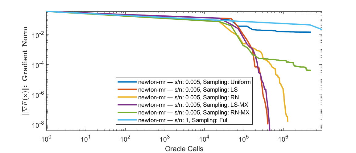
(a) $\|\nabla F(x_{k})\|$ vs. Oracle calls (Drive Diagnostics)

(b) $\|\nabla F(x_{k})\|$ vs. Oracle calls (Cover Type)

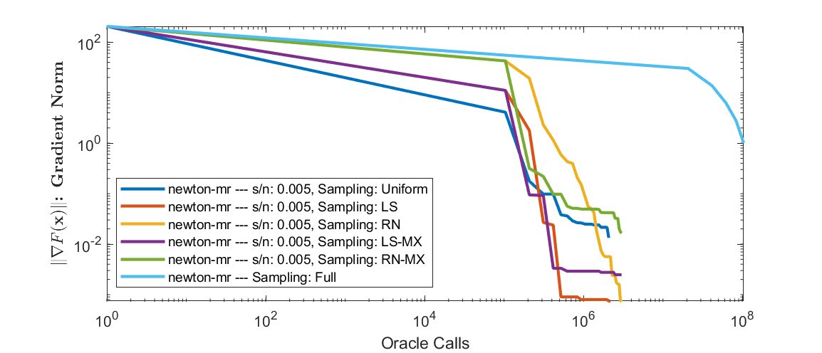
(c) $\|\nabla F(x_{k})\|$ vs. Oracle calls (UJIIndoorLoc)

Figure 1: Comparison of Newton-MR with various sampling schemes.

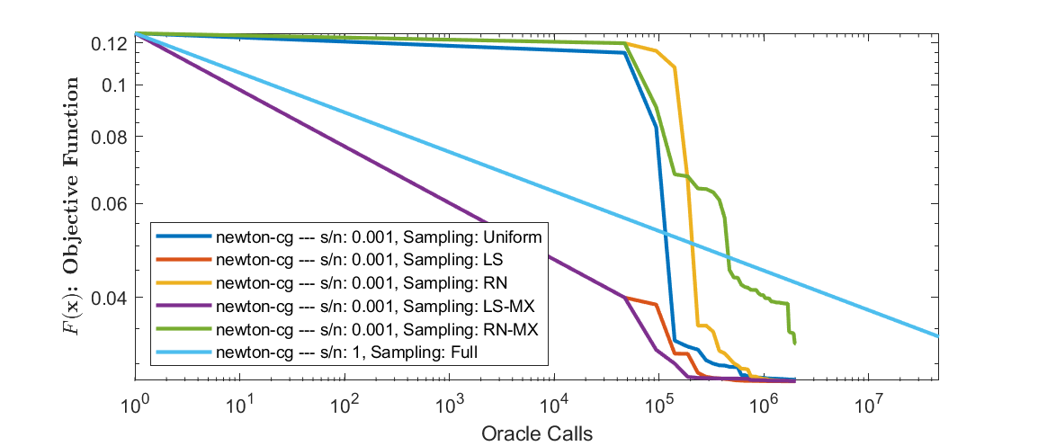
(a) $F(x_{k})$ vs. Oracle calls

(b) $\|\nabla F(x_{k})\|$ vs. Oracle calls

(c) $F(x_{k})$ vs. Oracle calls

(d) $F(x_{k})$ vs. Oracle calls

Figure 2: Comparison of (a) Newton-CG, (b) Newton-MR, and (c) Trust-region using various sampling schemes. (d) Performance of the hybrid sampling scheme.

Sub-sampling Schemes.

We focus on several sub-sampling strategies (all are done with replacement). Uniform: For this we have $p_{i}=1/n,\;i=1,\ldots,n$. Leverage Scores (LS): Complex leverage score sampling by considering the leverage scores of ${\mathbf{D}}^{1/2}{\mathbf{A}}$ as in Algorithm 1. Row Norms (RN): Row-norm sampling of ${\mathbf{D}}^{1/2}{\mathbf{A}}$ using 3 where $s(({\mathbf{D}}^{1/2}{\mathbf{A}})_{i})=|f_{i}{{}^{\prime\prime}}(\left\langle{\bf a}_{i},{\bf x}\right\rangle)|\left\|{\bf a}_{i}\right\|_{2}^{2}$. Mixed Leverage Scores (LS-MX): A mixed leverage score sampling strategy arising from a non-symmetric viewpoint of the product ${\mathbf{A}}^{{\mathchoice{\raisebox{0.0pt}{$\displaystyle\intercal$}}{\raisebox{0.0pt}{$\textstyle\intercal$}}{\raisebox{0.0pt}{$\scriptstyle\intercal$}}{\raisebox{0.0pt}{$\scriptscriptstyle\intercal$}}}}\left({\mathbf{D}}{\mathbf{A}}\right)$ using 2 with $s({\mathbf{A}}_{i})=\ell_{i}({\mathbf{A}})$ and $s(({\mathbf{D}}{\mathbf{A}})_{i})=\ell_{i}({\mathbf{D}}{\mathbf{A}})$. Mixed Norm Mixture (RN-MX): A mixed row-norm sampling strategy with the same non-symmetric viewpoint as in 2 with $s({\mathbf{A}}_{i})=\left\|({\mathbf{A}})_{i}\right\|$ and $s(({\mathbf{D}}{\mathbf{A}})_{i})=\left\|({\mathbf{D}}{\mathbf{A}})_{i}\right\|$. Hybrid Randomized-Deterministic (LS-Det): Sampling using Algorithm 2. Full: In this case, the exact Hessian is used.

Model Problems and Datasets.

We consider the task of binary classification using the non-linear least squares formulation of 1. Numerical experiments in this section are done using covertype, Drive Diagnostics, and UJIIndoorLoc from the UC Irvine ML Repository Dua and Graff [2017].

Performance Evaluation.

For Newton-MR, the convergence is measured by the norm of the gradient, and hence we evaluate it using various sampling schemes by plotting $\left\|\nabla F({{{\bf x}}_{k}})\right\|$ vs. the total number of oracle calls. For Newton-CG and trust-region, which guarantee descent in objective function, we plot $F({{{\bf x}}_{k}})$ vs. the total number of oracle calls. We deliberately choose not to use “wall-clock” time since it heavily depends on the implementation details and system specifications.

Comparison Among Various Sketching Techniques.

We present empirical evaluations of Uniform, LS, RN, LS-MX, RN-MX and Full sampling in the context of Newton-MR in Figure 1, and evaluation of all sampling schemes in Newton-CG, Newton-MR, Trust-region, and hybrid sampling on covertype in Figure 2. For all algorithms, LS and RN sampling amounts to a more efficient algorithm than that with LS-MX and RN-MX variants respectively, and at times this difference is more pronounced than other times, as predicted in Theorem 4. Meanwhile, LS and LS-MX often outperform RN and RN-MX, as proven in Theorem 1 and Theorem 2.

Evaluation of Hybrid Sketching Techniques.

To verify the result of Algorithm 2, we evaluate the performance of the trust-region algorithm by varying the terms involved in ${\mathbf{E}}$, where we call the rows with large leverage scores heavy, and denote the matrix formed by the heavy rows by ${\mathbf{E}}$. The matrix formed by the remaining rows is denoted by ${\mathbf{N}}$, see Theorem 3 for details. We do this for a simple splitting of ${\mathbf{H}}={\mathbf{E}}+{\mathbf{N}}$. We fix the overall sample size and change the fraction of samples that are deterministically picked in ${\mathbf{E}}$. The results are depicted in Figure 2. The value in brackets after LS-Det is the fraction of samples that are included in ${\mathbf{E}}$, i.e., deterministic samples. “LS-Det (0)” and “LS-Det (1)” correspond to ${\mathbf{E}}=\bm{0}$ and ${\mathbf{N}}=\bm{0}$, respectively. The latter strategy has been used in low rank matrix approximations [McCurdy, 2018]. As can be seen, the hybrid sampling approach is always competitive with, and at times strictly better than, LS-Det (0). As expected, LS-Det (1), which amounts to entirely deterministic samples, consistently performs worse. This can be easily attributed to the high bias of such a deterministic estimator.

3 Sketch-and-Solve Paradigm For Complex Regression

3.1 Theoretical Results

Recall the $\ell_{p}$-regression problem:

$$\min_{{\bf x}}\|{\mathbf{A}}{\bf x}-{\bf b}\|_{p}$$ (6)

Here we consider the complex version: ${\mathbf{A}}\in\mathbb{C}^{n\times d},{\bf b}\in\mathbb{C}^{n},{\bf x}\in\mathbb{C}^{d}$.

The inner product over the complex field can be embedded into a higher-dimensional real vector space. It suffices to consider the scalar case.

Lemma 1.

Let $x,y\in\mathbb{C}$ where $x=a+bi,y=c+di$, let $\phi:\mathbb{C}\to\mathbb{R}^{2}$ via $\phi(x)=\phi(a+bi)=[a\ \ b].$ Let $\sigma:\mathbb{C}\to\mathbb{R}^{2\times 2}$ via: $\sigma(y)=\sigma(c+di)=\begin{bmatrix}c&d\\ -d&c\end{bmatrix}$ . Then $\phi$ and $\sigma$ are bijections (between their domains and images), and we have $\phi(\bar{y}x)^{\mathchoice{\raisebox{0.0pt}{$\displaystyle\intercal$}}{\raisebox{0.0pt}{$\textstyle\intercal$}}{\raisebox{0.0pt}{$\scriptstyle\intercal$}}{\raisebox{0.0pt}{$\scriptscriptstyle\intercal$}}}=\sigma(y)\phi(x)^{\mathchoice{\raisebox{0.0pt}{$\displaystyle\intercal$}}{\raisebox{0.0pt}{$\textstyle\intercal$}}{\raisebox{0.0pt}{$\scriptstyle\intercal$}}{\raisebox{0.0pt}{$\scriptscriptstyle\intercal$}}}$

Proof of Lemma 1.

It is clear that $\phi,\sigma$ are bijections between their domains and images. $\sigma(y)\phi(x)^{\mathchoice{\raisebox{0.0pt}{$\displaystyle\intercal$}}{\raisebox{0.0pt}{$\textstyle\intercal$}}{\raisebox{0.0pt}{$\scriptstyle\intercal$}}{\raisebox{0.0pt}{$\scriptscriptstyle\intercal$}}}=\begin{bmatrix}c&d\\ -d&c\end{bmatrix}\begin{bmatrix}a\\ b\end{bmatrix}=\begin{bmatrix}ac+bd\\ cb-ad\end{bmatrix}=\phi(\bar{y}x)^{\mathchoice{\raisebox{0.0pt}{$\displaystyle\intercal$}}{\raisebox{0.0pt}{$\textstyle\intercal$}}{\raisebox{0.0pt}{$\scriptstyle\intercal$}}{\raisebox{0.0pt}{$\scriptscriptstyle\intercal$}}}.$ ∎

We apply $\sigma$ to each entry in ${\mathbf{A}}$ and concatenate in the natural way. Abusing notation, we then write: ${\mathbf{A}}^{\prime}=\sigma({\mathbf{A}})\in\mathbb{R}^{2n\times 2d}.$ Similarly, we write ${\bf x}^{\prime}=\phi({\bf x})\in\mathbb{R}^{2d},\ {\bf b}^{\prime}=\phi({\bf b})\in\mathbb{R}^{2d}.$

Fact 1.

For $1\leq p<q\leq\infty$ and ${\bf x}\in\mathbb{R}^{d}$, we have $\|{\bf x}\|_{q}\leq\|{\bf x}\|_{p}\leq d^{1/p-1/q}\|{\bf x}\|_{q}.$

Fact 2.

An $\ell_{p}$ Auerbach basis is well-conditioned and always exists.

Definition 4.

Let ${\bf x}\in\mathbb{R}^{2d}$ for some $d\in\mathbb{N}$. Define $\left|\mspace{-1.8mu}\left|\mspace{-1.8mu}\left\lvert{\bf x}\right|\mspace{-1.8mu}\right|\mspace{-1.8mu}\right|_{p,2}=\left(\sum_{i=0}^{d-1}\left({\bf x}_{2i+1}^{2}+{\bf x}_{2i+2}^{2}\right)^{p/2}\right)^{1/p}.$ Note that letting ${\bf x}\in\mathbb{C}^{d}$, we have $\|{\bf x}\|_{p}=\left|\mspace{-1.8mu}\left|\mspace{-1.8mu}\left\lvert\phi({\bf x})\right|\mspace{-1.8mu}\right|\mspace{-1.8mu}\right|_{p,2}$.

By Definition 4, we can “lift” the original $\ell_{p}$-regression to $\mathbb{R}^{2d}$ and solve $\min_{\phi({\bf x})\in\mathbb{R}^{2d}}\left|\mspace{-1.8mu}\left|\mspace{-1.8mu}\left\lvert\sigma({\mathbf{A}})\phi({\bf x})-\phi({\bf b})\right|\mspace{-1.8mu}\right|\mspace{-1.8mu}\right|_{p,2}$ instead of 6. This equivalence allows us to consider sketching techniques on real matrices with proper modification. See Algorithm 3 for details. In turn, such an embedding gives an arbitrarily good approximation with high probability, as shown in Theorem 5.

Algorithm 3 Fast Algorithm for Complex $\ell_{p}$-regression

1:  Input: ${\mathbf{A}}^{\prime}\in\mathbb{R}^{2n\times 2d},{\bf b}^{\prime}\in\mathbb{R}^{2d}$, precision $\epsilon>0$, $p\in[1,\infty]$

2:  Set $t\geq C\frac{\log(1/\epsilon){\bf poly}(d)}{\epsilon^{2}}$, $\gamma=d^{-1/q-1}$, $\sigma=\frac{\sqrt{\pi}}{2^{p/2}\Gamma((p+1)/2)}$, $\mathcal{P}=\{P=(2i+1,2i+2)\in\mathbb{R}^{2},\forall i\in\{0,\ldots,d-1\}\}$

3:  if $p\neq\infty$ then

4:     Compute the $\ell_{p}$ leverage score $\{\ell([{\mathbf{A}}^{\prime}_{1}\ \ {\bf b}^{\prime}_{1}]),\ldots,\ell([{\mathbf{A}}^{\prime}_{n}\ \ {\bf b}^{\prime}_{n}])\}$ for each row of $[{\mathbf{A}}^{\prime}\ \ {\bf b}^{\prime}]$

5:     Let $\mathcal{P}_{h}$ be the collection of $P=(a,b)\in\mathcal{P}$ such that $\ell([{\mathbf{A}}^{\prime}_{a}\ \ {\bf b}^{\prime}_{a}])\geq\gamma$ or $\ell([{\mathbf{A}}^{\prime}_{b}\ \ {\bf b}^{\prime}_{b}])\geq\gamma$. Denote the collection of all other pairs $\mathcal{P}_{l}$

6:     Rearrange $[{\mathbf{A}}^{\prime}\ \ {\bf b}^{\prime}]$ such that the rows in $\mathcal{P}_{h}$ are on top

7:     for Each $P_{i}\in\mathcal{P}_{h}$ do

8:         Sample a Gaussian random matrix ${\mathbf{G}}_{P_{i}}\in\mathbb{R}^{t\times 2}$, where each entry follows $\mathcal{N}(0,\sigma^{2})$

9:     for Each $Q_{i}\in\mathcal{P}_{l}$ do

10:         Sample Gaussian random matrix ${\mathbf{G}}_{Q_{i}}\in\mathbb{R}^{1\times 2}$, where each entry follows $\mathcal{N}(0,\sigma^{2})$

11:     Define a block diagonal matrix ${\mathbf{G}}={\textnormal{diag}}({\mathbf{G}}_{P_{1}},\ldots,{\mathbf{G}}_{P_{|\mathcal{P}_{h}|}},{\mathbf{G}}_{Q_{1}},\ldots,{\mathbf{G}}_{Q_{|\mathcal{P}_{l}|}})$

12:     Output: $\|{\mathbf{G}}{\mathbf{A}}^{\prime}{\bf y}-{\mathbf{G}}{\bf b}^{\prime}\|_{p}$

13:  else

14:     for Each $P_{i}\in\mathcal{P}$ do

15:         Sample Gaussian matrix ${\mathbf{G}}_{P_{i}}\in\mathbb{R}^{s\times 2}$ with entries from $\mathcal{N}(0,\frac{\pi}{2})$, where $s=\mathcal{O}\left(\frac{\log(1/\epsilon)}{\epsilon^{2}}\right)$

16:         Let ${\mathbf{R}}_{P_{i}}\in\mathbb{R}^{2^{s}\times s}$ where each row of ${\mathbf{R}}_{P_{i}}$ is a vector in $\{-1,+1\}^{s}$

17:     Let ${\mathbf{R}}={\textnormal{diag}}({\mathbf{R}}_{1},\ldots,{\mathbf{R}}_{|\mathcal{P}|})$, ${\mathbf{G}}={\textnormal{diag}}({\mathbf{G}}_{1},\ldots,{\mathbf{G}}_{|\mathcal{P}|})$

18:     Output: $\|{\mathbf{R}}{\mathbf{G}}{\mathbf{A}}^{\prime}{\bf y}-{\mathbf{R}}{\mathbf{G}}{\bf b}^{\prime}\|_{\infty}$

Theorem 5.

Let ${\mathbf{A}}\in\mathbb{C}^{n\times d},{\bf b}\in\mathbb{C}^{n}$. Then Algorithm 3 with input ${\mathbf{A}}^{\prime}:=\sigma({\mathbf{A}})$ and ${\bf b}^{\prime}:=\phi({\bf b})$ returns a regression instance whose optimizer is an $\epsilon$ approximation to 6, with probability at least $0.98$. The total time complexity for $p\in[1,\infty)$ is $\mathcal{O}({\bf nnz}({\mathbf{A}})+{\bf poly}(d/\epsilon))$; for $p=\infty$ it is $\mathcal{O}(2^{\tilde{}\mathcal{O}(1/\epsilon^{2})}{\bf nnz}({\mathbf{A}}))$. The returned instance can then be optimized by any $\ell_{p}$-regression solver.

Proof.

For simplicity, we let ${\mathbf{A}}\in\mathbb{R}^{2n\times 2d}$ to avoid repeatedly writing the prime symbol in ${\mathbf{A}}^{\prime}$.

Let ${\bf y}\in\mathbb{R}^{2n}$ be arbitrary. Let $P,\mathcal{P},\mathcal{P}_{l},\mathcal{P}_{h}$ be as defined in Algorithm 3. We say a pair $P=(a,b)$ is heavy if $P\in\mathcal{P}_{h}$, and light otherwise.

As an overview, when $p\in[1,\infty)$, for the heavy pairs, we use a large Gaussian matrix and apply Dvoretsky’s theorem to show the $\left|\mspace{-1.8mu}\left|\mspace{-1.8mu}\left\lvert\cdot\right|\mspace{-1.8mu}\right|\mspace{-1.8mu}\right|_{p,2}$ norm is preserved. For the light pairs, we use a single Gaussian vector and use Bernstein’s concentration. This is intuitive since the heavy pairs represent the important directions in ${\mathbf{A}}$, and hence we need more Gaussian vectors to preserve their norms more accurately; but the light pairs are less important and so the variance of the light pairs can be averaged across multiple coordinates. Hence, using one Gaussian vector suffices for each light pair. For $p=\infty$, we need to preserve the $\ell_{2}$ norm of every pair, and so in this case we apply Dvoretsky’s theorem to sketch every single pair in $\mathcal{P}$.

We split the analysis into two cases: $p\in[1,\infty)$ and $p=\infty$. In the main text we only present $p\in[1,\infty)$ and defer the other case to the appendix.

Case 1: $p\in[1,\infty)$.

For light rows:

Let ${\mathbf{U}}$ be an Auerbach basis of ${\mathbf{A}}$ and ${\bf y}={\mathbf{U}}{\bf x}$, where ${\bf x}\in\mathbb{R}^{d}$ is arbitrary. Then for any row index $i\in[n]$:

$$|{\bf y}_{i}|=|{\mathbf{U}}_{i}{\bf x}|\leq\|{\mathbf{U}}_{i}\|_{p}\|{\bf x}\|_{q}\leq d^{1/q}\|{\mathbf{U}}_{i}\|_{p}\|{\bf y}\|_{p}\Longrightarrow\frac{d^{-1/q}|{\bf y}_{i}|}{\|{\bf y}\|_{p}}\leq\|{\mathbf{U}}_{i}\|_{p}$$

where the first step is because the Auerbach basis satisfies $\|{\mathbf{U}}{\bf x}\|_{p}=\|{\bf y}\|_{p}\geq d^{-1/q}\|{\bf x}\|_{q}$. This implies that if $|{\bf y}_{i}|\geq\gamma d^{1/q}\|{\bf y}\|_{p}$, then $\|{\mathbf{U}}_{i}\|_{p}\geq\gamma$. Hence, by definition of $\gamma$, if $\|{\mathbf{U}}_{i}\|_{p}\leq d^{-1/q-1}$, then $|{\bf y}_{i}|\leq d^{-1}\|{\bf y}\|_{p}$.

For any light pair $P=(a,b)$, we sample two i.i.d. Gaussians ${\bf g}_{P}=({\bf g}_{a},{\bf g}_{b})$ from $\mathcal{N}(0,\sigma^{2})$ where $\sigma=\frac{\sqrt{\pi}}{2^{p/2}\Gamma((p+1)/2)}$. Since ${\bf g}_{a}{\bf y}_{a}+{\bf g}_{b}{\bf y}_{b}\sim\mathcal{N}(0,\|{\bf y}_{P}\|_{2}^{2}\sigma^{2})$, we have $\mathbb{E}[|{\bf g}_{a}{\bf y}_{a}+{\bf g}_{b}{\bf y}_{b}|^{p}]=\|{\bf y}_{P}\|_{2}^{p}$.

Let $\mathcal{P}_{l}$ be the set of all light pairs. We have, $\mathbb{E}[\sum_{P\in\mathcal{P}_{l}}|\langle{\bf g}_{P},{\bf y}_{P}\rangle|^{p}]=\sum_{P\in\mathcal{P}_{l}}\|{\bf y}_{P}\|_{2}^{P}.$

Let random variable $Z_{P}=|\langle{\bf g}_{P},{\bf y}_{P}\rangle|$. This is $\sigma^{2}\|{\bf y}_{P}\|_{2}^{2}$-sub-Gaussian (the parameter here can be improved by subtracting $\mu_{Z_{P}}^{2}$).

Define event $\mathcal{A}$ to be : $\max_{P\in\mathcal{P}_{l}}Z_{P}^{p}\geq\mathcal{O}((\log(|\mathcal{P}_{l}|)+{\bf poly}(d))^{p})\triangleq t$. Since the $Z_{P}$ variables are sub-Gaussian and $p\geq 1$, we have that $(\cdot)^{p}$ is monotonically increasing, so we can use the standard sub-Gaussian bound to get

$$P(\mathcal{A})<\exp\left(-{\bf poly}(d)\right).$$ (7)

Note that $p$ is a constant, justifying the above derivation.

Also note that $\text{Var}(Z_{P})=\mathcal{O}(\|{\bf y}_{P}\|^{2p}_{2})$. Condition on $\neg\mathcal{A}$. By Bernstein’s inequality, we have:

$$\begin{split}&P\left(\left|\sum_{P\in\mathcal{P}_{l}}Z_{P}^{p}-\mathbb{E}[|\sum_{P\in\mathcal{P}_{l}}Z_{P}^{p}|]\right|>\epsilon\mathbb{E}[|\sum_{P\in\mathcal{P}}Z_{P}^{p}|]\right)\\ =&P\left(\left|\sum_{P\in\mathcal{P}_{l}}Z_{P}^{p}-\sum_{P\in\mathcal{P}_{l}}\|{\bf y}_{P}\|_{2}^{p}\right|>\epsilon\sum_{P\in\mathcal{P}}\|{\bf y}_{P}\|_{2}^{p}\right)\\ \leq&\exp\left(-\frac{\epsilon^{2}(\sum_{P\in\mathcal{P}}\|{\bf y}_{P}\|_{2}^{p})^{2}}{\sum_{P\in\mathcal{P}_{l}}\|{\bf y}_{P}\|^{2p}_{2}+\epsilon t\sum_{P\in\mathcal{P}_{l}}\|{\bf y}_{P}\|_{2}^{p}}\right)\\ \leq&\exp\left(-\mathcal{O}\left(\frac{\epsilon^{2}(\sum_{P\in\mathcal{P}}\|{\bf y}_{P}\|_{2}^{p})^{2}}{\sum_{P\in\mathcal{P}_{l}}\|{\bf y}_{P}\|^{2p}_{2}}\right)\right)\\ \leq&\exp\left(-\mathcal{O}(\epsilon^{2}/\gamma)\right)=\exp\left(\mathcal{O}(-\epsilon^{2}d\log d)\right)\end{split}$$ (8)

where the last step follows from the definition of light pairs. Using that if for all $P=(a,b)\in\mathcal{P}_{l}$, $|{\bf y}_{a}|,|{\bf y}_{b}|<\mathcal{O}(d^{-1})\|{\bf y}\|_{p}$, then $\|{\bf y}_{P}\|_{2}^{p}<\mathcal{O}(d^{-1})\|{\bf y}\|_{p}^{p}$, we have

$$\sum_{P\in\mathcal{P}_{l}}\|{\bf y}_{P}\|_{2}^{2p}\leq\frac{1}{\mathcal{O}(d^{-1})}\mathcal{O}(d^{-2})\|{\bf y}\|_{p}^{2p}=\mathcal{O}(d^{-1})\|{\bf y}\|_{p}^{2p}.$$

Since $\sum_{P\in\mathcal{P}}\|{\bf y}_{P}\|_{2}^{p}\leq\mathcal{O}(\|{\bf y}\|_{p}^{p})$, we will have $\frac{(\sum_{P\in\mathcal{P}}\|{\bf y}_{P}\|_{2}^{p})^{2}}{\sum_{P\in\mathcal{P}_{l}}\|{\bf y}_{P}\|^{2p}_{2}}=\mathcal{O}(d)$.

Net argument. In the above derivation, we fix a vector ${\bf y}\in\mathbb{R}^{2n}$. Hence for the above argument to hold for all pairs, a naïve argument will not work since there are an infinite number of pairs. However, note that each pair lives in a two-dimensional subspace. Hence, we can take a finer union bound over $\mathcal{O}((1+\epsilon)^{2}/\epsilon^{2})$ items in a two-dimensional $\ell_{2}$ space using a net argument. This argument is standard, see, e.g., [Woodruff et al., 2014, Chapter 2].

Using the net argument, 8 and 7 holds with probability at least $1-\mathcal{O}(e^{-d})$ for all ${\bf y}\in\mathbb{R}^{2n}$ simultaneously. In particular, with probability at least $0.99$:

$$\sum_{P\in\mathcal{P}_{l}}|\langle{\bf g}_{P},{\bf y}_{P}\rangle|^{p}-\sum_{P\in\mathcal{P}_{l}}\|{\bf y}_{P}\|_{2}^{p}\in(\pm\epsilon)\sum_{P\in\mathcal{P}}\|{\bf y}_{P}\|_{2}^{p}.$$ (9)

For heavy rows:

Since the $\ell_{p}$ leverage scores sum to $d$, there can be at most $d/\gamma={\bf poly}(d)$ heavy rows. For each pair $P\in\mathcal{P}_{h}$, we construct a Gaussian matrix ${\mathbf{G}}_{P}\in\mathbb{R}^{s\times 2}$, where $s={\bf poly}(d/\epsilon)$. Applying Dvoretsky’s theorem for $\ell_{p}$ (Paouris et al. [2017] Theorem 1.2), with probability at least $0.99$, for all $2$-dimensional vectors ${\bf y}_{P}$, $\|{\mathbf{G}}_{P}{\bf y}_{P}\|_{p}=(1\pm\epsilon)\|{\bf y}_{P}\|_{2}$. Hence,

$$\sum_{P\in\mathcal{P}_{h}}\|{\mathbf{G}}_{P}{\bf y}_{P}\|_{p}^{p}=(1\pm\Theta(\epsilon))\sum_{P\in\mathcal{P}_{h}}\|{\bf y}_{P}\|_{2}^{p}.$$ (10)

Combining 9 and 10, we have with probability at least $0.98$, for all ${\bf y}\in\mathbb{R}^{2n}$:

$$\|{\mathbf{G}}{\bf y}\|_{p}^{p}=(1\pm\Theta(\epsilon))\sum_{P\in\mathcal{P}}\|{\bf y}_{P}\|_{2}^{p}=(1\pm\Theta(\epsilon))\left|\mspace{-1.8mu}\left|\mspace{-1.8mu}\left\lvert{\bf y}\right|\mspace{-1.8mu}\right|\mspace{-1.8mu}\right|_{p,2}^{p}$$

Letting ${\bf y}={\mathbf{U}}{\bf x}-{\bf b}$ and taking the $1/p$-th root, we obtain the final claim.

Case 2: $p=\infty$.

In this case, we first construct a sketch ${\mathbf{G}}$ to embed every pair into $\ell_{1}$. That is, for all $P\in\mathcal{P}$, construct a Gaussian matrix ${\mathbf{G}}_{p}\in\mathbb{R}^{\mathcal{O}\left(\frac{\log(1/\epsilon)}{\epsilon^{2}}\right)\times 2}$. By Dvoretsky’s theorem, with probability at least $0.99$, for all ${\bf y}_{P}\in\mathbb{R}^{2}$, we have $\|{\mathbf{G}}_{P}{\bf y}_{P}\|_{1}=(1\pm\epsilon)\|{\bf y}_{P}\|_{2}$. Hence

$$\begin{split}\text{For all ${\bf y}\in\mathbb{R}^{2n}$ and any $P\in\mathcal{P}$: }\max_{P\in\mathcal{P}}\|{\mathbf{G}}_{P}{\bf y}_{P}\|_{1}=\max_{P\in\mathcal{P}}(1\pm\epsilon)\|{\bf y}_{P}\|_{2}=\left|\mspace{-1.8mu}\left|\mspace{-1.8mu}\left\lvert{\bf y}\right|\mspace{-1.8mu}\right|\mspace{-1.8mu}\right|_{\infty,2}\end{split}$$ (11)

However, we do not want to optimize the left hand side directly.

Recall that by construction ${\mathbf{G}}={\textnormal{diag}}({\mathbf{G}}_{1},\ldots,{\mathbf{G}}_{|\mathcal{P}|})$ is a block diagonal matrix.

Construct ${\mathbf{R}}$ as in Algorithm 3. By Indyk [2001], for all $P\in\mathcal{P}$, ${\mathbf{R}}_{P}$ is an isometric embedding $\ell_{1}\hookrightarrow\ell_{\infty}$, i.e., for all ${\bf y}_{P}\in\mathbb{R}^{2}$: $\|{\mathbf{R}}_{P}{\mathbf{G}}_{P}{\bf y}_{P}\|_{\infty}=\|{\mathbf{G}}_{P}{\bf y}_{P}\|_{1}.$

Combining this with 11, we get that with probability at least $0.99$ for all ${\bf y}\in\mathbb{R}^{2n}$:

$$\|{\mathbf{R}}{\mathbf{G}}{\bf y}\|_{\infty}=(1\pm\Theta(\epsilon))\left|\mspace{-1.8mu}\left|\mspace{-1.8mu}\left\lvert{\bf y}\right|\mspace{-1.8mu}\right|\mspace{-1.8mu}\right|_{\infty,2}.$$

Letting ${\bf y}={\mathbf{U}}{\bf x}-{\bf b}$, we obtain the final claim.

Running time.

For $p\in[1,\infty)$, calculating a well-conditioned basis takes $\mathcal{O}({\bf nnz}({\mathbf{A}})+{\bf poly}(d/\epsilon))$ time. Since ${\mathbf{G}}$ is a block diagonal matrix and ${\mathbf{A}}$ is sparse, computing ${\mathbf{G}}{\mathbf{A}}$ takes $\mathcal{O}({\bf nnz}({\mathbf{A}})+{\bf poly}(d/\epsilon))$ time. Calculating ${\mathbf{G}}{\bf b}$ takes $n+{\bf poly}(d/\epsilon)$ time. Minimizing $\|{\mathbf{G}}{\mathbf{A}}{\bf x}-{\mathbf{G}}{\bf b}\|$ up to a $(1+\epsilon)$ factor takes $\mathcal{O}({\bf nnz}({\mathbf{A}})+{\bf poly}(d/\epsilon))$ time. Using the fact that $n<{\bf nnz}({\mathbf{A}})$, the total running time is $\mathcal{O}({\bf nnz}({\mathbf{A}})+{\bf poly}(d/\epsilon))$.

For the case of $p=\infty$, note that ${\mathbf{R}}$ is also a block diagonal matrix, so ${\mathbf{R}}{\mathbf{G}}$ can be computed by multiplying the corresponding blocks, which amounts to $\mathcal{O}(2^{\tilde{}\mathcal{O}(1/\epsilon^{2})}n\frac{\log(1/\epsilon)}{\epsilon^{2}})$ time. ${\mathbf{A}}$ is sparse and ${\mathbf{R}}{\mathbf{G}}$ is a block matrix so computing ${\mathbf{R}}{\mathbf{G}}{\mathbf{A}}$ takes another $\mathcal{O}(2^{\tilde{}\mathcal{O}(1/\epsilon^{2})}{\bf nnz}({\mathbf{A}}))$ time. Computing ${\mathbf{R}}{\mathbf{G}}{\bf b}$ takes $\mathcal{O}(2^{\tilde{}\mathcal{O}(1/\epsilon^{2})}n\frac{\log(1/\epsilon)}{\epsilon^{2}})$ time. Since $n<{\bf nnz}({\mathbf{A}})$, in total these take $\mathcal{O}(2^{\tilde{}\mathcal{O}(1/\epsilon^{2})}{\bf nnz}({\mathbf{A}}))$ time. This concludes the proof. ∎

Remark 3.

Definition 4 shows for sketching complex vectors in the $\ell_{p}$ norm, all one needs is an embedding $\ell_{2}\hookrightarrow\ell_{p}$. In particular, for complex $\ell_{2}$-regression, the identity map is such an embedding with no distortion. Hence, complex $\ell_{2}$-regression can be sketched exactly as for real-valued $\ell_{2}$-regression, while for other complex $\ell_{p}$-regression the transformation is non-trivial.

3.2 Numerical Evaluation

We evaluate the performance of our proposed embedding for $\ell_{1}$ and $\ell_{\infty}$ regression on synthetic data. With ${\mathbf{A}}\in\mathbb{C}^{100\times 50},{\bf b}\in\mathbb{C}^{100}$, we solve $\min_{{\bf x}\in\mathbb{C}^{50}}\|{\mathbf{A}}{\bf x}-{\bf b}\|_{1}$ or $\min_{{\bf x}\in\mathbb{C}^{50}}\|{\mathbf{A}}{\bf x}-{\bf b}\|_{\infty}$. Each entry of ${\mathbf{A}}$ and ${\bf b}$ is sampled from a standard normal distribution (the real and imaginary coefficients are sampled according to this distribution independently). Instead of picking the heavy ($\mathcal{P}_{h}$) and light ($\mathcal{P}_{l}$) pairs , we construct a $t\times 2$ (or $s\times 2$ if $p=\infty$) Gaussian matrix for each pair (that is, we treat all pairs as heavy), as it turns out in the experiments that very small $t$ or $s$ is sufficient. For $\ell_{1}$ complex regression, we test with $t=2,4,6,8,10,20$, and the result is shown in Figure 3(a). For $\ell_{\infty}$ complex regression, we test with $s=2,3,4,5,6$ as shown in Figure 3(b). In both figures, the $x$-axis represents our choice of $t$ or $s$, and the $y$-axis is the approximation error $\|\hat{\bf x}-{\bf x}^{*}\|_{2}$, where $\hat{\bf x}$ is the minimizer of our sketched regression problem.

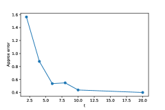
(a) $\ell_{1}$ regression

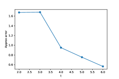
(b) $\ell_{\infty}$ regression

Figure 3: Approximation error of sketched $\ell_{p}$ regression with complex entries.

4 Sketching Vector-Matrix-Vector Queries

The sketches in Section 2 can also be used for vector-matrix-vector queries, but they are sub-optimal when there are a lot of cancellations. For example, if we have ${\mathbf{A}}^{\top}{\mathbf{D}}{\mathbf{A}}=\sum_{i=1}^{n}d_{i}{\bf a}_{i}{\bf a}_{i}^{\top}$ where ${\bf a}_{1}={\bf a}_{2}=\cdots={\bf a}_{n}$, $d_{1}=d_{2}=\cdots d_{n/2}$, and $d_{n/2+1}=d_{n/2+2}=\cdots=d_{n}$, then ${\mathbf{A}}^{\top}{\mathbf{D}}{\mathbf{A}}=0$, yet our sampling techniques need their number of rows to scale with $\|{\mathbf{A}}^{\top}|{\mathbf{D}}|{\mathbf{A}}\|_{F}$, which can be arbitrarily large. In this section, we give a sketching technique for vector-matrix-vector product queries that scales with $\|{\mathbf{A}}^{\top}{\mathbf{D}}{\mathbf{A}}\|_{F}$ instead of $\|{\mathbf{A}}^{\top}|{\mathbf{D}}|{\mathbf{A}}\|_{F}$. Therefore, for vector-matrix-vector product queries, this new technique works well, even if the matrices are complex. Such queries are widely used, including standard graph queries and independent set queries [Rashtchian et al., 2020].

In particular, we consider a vector-matrix-vector product query ${\bf u}^{\top}{\mathbf{M}}{\bf v}$, where ${\mathbf{M}}={\mathbf{A}}^{\top}{\mathbf{B}}=\sum_{i=1}^{n}{\bf a}_{i}{\bf b}_{i}^{\top}$ has a tensor product form, ${\bf a}_{i},{\bf b}_{i}\in\mathbb{C}^{d}$, for all $i\in[n]$. One has to either sketch ${\mathbf{M}}$ or compute ${\mathbf{M}}$ first. Then the queries ${\bf u}$ and ${\bf v}$ arrive [Andoni et al., 2016]. In reality, this may be due to the fact that $n\gg d$ and one cannot afford to store ${\mathbf{A}}$ and ${\mathbf{B}}$. Our approach is interesting when ${\mathbf{M}}$ is non-PSD and ${\mathbf{A}},{\mathbf{B}}$ might be complex. This can indeed happen, for example, in a graph Laplacian with negative weights [Chen et al., 2016].

Algorithm 4 Tensor Sketch For Vector-Matrix-Vector Products

1:  Input: $\{{\bf a}_{i}\}_{i=1}^{n},\{{\bf b}_{i}\}_{i=1}^{n}\subseteq\mathbb{C}^{d},{\bf u},{\bf v}\in\mathbb{C}^{d}$

2:  Let ${\mathbf{S}}:\mathbb{C}^{d}\otimes\mathbb{C}^{d}\to\mathbb{C}^{k}$ be a TensorSketch [Pham and Pagh, 2013] with $k$ hash buckets.

3:  Compute ${\bf q}=\sum_{i=1}^{n}{\mathbf{S}}({\bf a}_{i}\otimes{\bf b}_{i})\in\mathbb{C}^{k}$.

4:  Compute ${\bf p}={\mathbf{S}}({\bf u}\otimes{\bf v})\in\mathbb{C}^{k}$.

5:  Output: $\langle{\bf p},{\bf q}\rangle$

Theorem 6.

With probability at least $0.99$, for given input vectors ${\bf u},{\bf v}\in\mathbb{C}^{d}$, ${\mathbf{A}},{\mathbf{B}}\in\mathbb{C}^{n\times d}$, Algorithm 4 returns an answer $z$ such that $\left|{\bf z}-{\bf u}^{\top}{\mathbf{A}}^{\top}{\mathbf{B}}{\bf v}\right|\leq\epsilon$ in time $\tilde{}\mathcal{O}\left({\bf nnz}({\mathbf{A}})+\frac{n\|{\bf v}\|_{2}^{2}\|{\bf u}\|_{2}^{2}\|{\mathbf{A}}^{\top}{\mathbf{B}}\|_{F}^{2}}{\epsilon^{2}}\right)$.

Proof.

It is known that TensorSketches are unbiased, that is,

$$\mathbb{E}[\langle{\mathbf{S}}({\mathbf{A}}^{\top}{\mathbf{B}}),{\mathbf{S}}({\bf u}\otimes{\bf v})\rangle]={\bf u}^{\top}{\mathbf{A}}^{\top}{\mathbf{B}}{\bf v},$$

where ${\mathbf{S}}({\mathbf{A}}^{\top}{\mathbf{B}})=\sum_{i=1}^{n}{\mathbf{S}}({\bf a}_{i},{\bf b}_{i})$ follows from the linearity of TensorSketch Pham and Pagh [2013]. The variance is bounded by

$$\operatorname{Var}\left(\langle{\mathbf{S}}({\mathbf{A}}^{\top}{\mathbf{B}}),{\mathbf{S}}({\bf u}\otimes{\bf v})\rangle\right)\leq\mathcal{O}\left(\frac{1}{k}\|{\bf v}\|_{2}^{2}\|{\bf u}\|_{2}^{2}\|{\mathbf{A}}^{\top}{\mathbf{B}}\|_{F}^{2}\right),$$

see, e.g., Pham and Pagh [2013]. By Chebyshev’s inequality, setting $k=\mathcal{O}\left(\frac{\|{\bf v}\|_{2}^{2}\|{\bf u}\|_{2}^{2}\|{\mathbf{A}}^{\top}{\mathbf{B}}\|_{F}^{2}}{\epsilon^{2}}\right)$ produces an estimate of ${\bf u}^{\top}{\mathbf{A}}^{\top}{\mathbf{B}}{\bf v}$ with an additive error $\epsilon$.

Note that computing the sketches ${\mathbf{S}}({\mathbf{A}}^{\top}{\mathbf{B}})$ takes time ${\bf nnz}({\mathbf{A}})+{\bf nnz}({\mathbf{B}})+nk\log k$, and computing the inner product $\langle{\mathbf{S}}({\mathbf{A}}^{\top}{\mathbf{B}}),{\mathbf{S}}({\bf u}\otimes{\bf v})\rangle$ takes only $k$ time. As a comparison, computing ${\bf u}^{\top}{\mathbf{A}}^{\top}{\mathbf{B}}{\bf v}$ naïvely takes $nd^{2}+O(d^{2})$ time, which can be arbitrarily worse than our sketched version. Note that it is prohibitive in our setting to compute ${\bf u}^{\top}{\mathbf{A}}^{\top}$ and ${\mathbf{B}}{\bf v}$ separately. ∎

5 Conclusion

Our work highlights the many places where non-PSD matrices and their “square roots”, which are complex matrices, arise in optimization and randomized numerical linear algebra. We give novel dimensionality reduction methods for such matrices in optimization, the sketch-and-solve paradigm, and for vector-matrix-vector queries. These methods can be used for approximating indefinite Hessian matrices, which constitute a major bottleneck for second-order optimization. We also propose a hybrid sampling method for matrices that satisfy a relaxed RIP condition. We verify these numerically using Newton-CG, trust region, and Newton-MR algorithms. We also show how to reduce complex $\ell_{p}$-regression to real $\ell_{p}$-regression in a black box way using random linear embeddings, showing that the many sketching techniques developed for real matrices can be applied to complex matrices as well. In addition, we also present how to efficiently sketch complex matrices for vector-matrix-vector queries.

Acknowledgments: The authors would like to thank partial support from NSF grant No. CCF-181584, Office of Naval Research (ONR) grant N00014-18-1-256, and a Simons Investigator Award.

Appendix A Algorithms

Algorithm 5 Newton-CG With Inexact Hessian

  Input: Starting point ${{{\bf x}}_{0}}$, line-search parameter $0<\rho<1$

  for $k=0,1,2,\ldots$ until convergence do

     (approximately) Solve the following sub-problem using CG

$${{\mathbf{H}}_{k}}{\bf p}=-{{{\bf g}}_{k}}$$

     Find ${{\alpha}_{k}}$ such that

$$F({{{\bf x}}_{k+1}})\leq F({{{\bf x}}_{k}})+\rho\alpha_{k}\left\langle{{{\bf p}}_{k}},{{{\bf g}}_{k}}\right\rangle$$

     Update ${\bf x}_{k+1}={{{\bf x}}_{k}}+{{\alpha}_{k}}{{{\bf p}}_{k}}$

  Output: ${{{\bf x}}_{k}}$

Algorithm 6 Newton-MR With Inexact Hessian

1:  Input: Starting point ${{{\bf x}}_{0}}$, line-search parameter $0<\rho<1$

2:  for $k=0,1,2,\ldots$ until convergence do

3:     (approximately) Solve the following sub-problem

$$\min_{{\bf p}\in^{d}}\leavevmode\nobreak\ \leavevmode\nobreak\ \|{\bf p}\|\;\;\text{subject to}\;\;{\bf p}\in\operatorname*{arg\,min}_{\widehat{{\bf p}}\in\mathbb{R}^{d}}\left\|{{\mathbf{H}}_{k}}\widehat{{\bf p}}+{{{\bf g}}_{k}}\right\|.$$

4:     Find ${{\alpha}_{k}}$ such that

$$\left\|{{{\bf g}}_{k+1}}\right\|^{2}\leq\left\|{{{\bf g}}_{k}}\right\|^{2}+2\rho\alpha_{k}\left\langle{{{\bf p}}_{k}},{{\mathbf{H}}_{k}}{{{\bf g}}_{k}}\right\rangle$$

5:     Update ${\bf x}_{k+1}={{{\bf x}}_{k}}+{{\alpha}_{k}}{{{\bf p}}_{k}}$

6:  Output: ${{{\bf x}}_{k}}$

Algorithm 7 Trust Region with Inexact Hessian

1:  Input: Starting point ${{{\bf x}}_{0}}$, initial radius $0<\Delta_{0}<\infty$, hyper-parameters $\eta\in(0,1),\gamma>1$

2:  for $k=0,1,\ldots$ do

3:     Set the approximate Hessian, ${{\mathbf{H}}_{k}}$, as in (4)

4:     if converged then

5:         Return ${{{\bf x}}_{k}}$.

6:     (approximately) solve the following sub-problem

$$\min_{\|{\bf p}\|\leq\Delta_{k}}m_{k}({\bf p})\triangleq\left\langle\nabla F({{{\bf x}}_{k}}),{\bf p}\right\rangle+\frac{1}{2}\left\langle{\bf p},{{\mathbf{H}}_{k}}{\bf p}\right\rangle,$$

7:     Set $\rho_{k}\triangleq\dfrac{F({{{\bf x}}_{k}}+{{{\bf p}}_{k}})-F({{{\bf x}}_{k}})}{m_{t}({{{\bf p}}_{k}})}$

8:     if $\rho_{k}\geq\eta$ then

9:         ${{{\bf x}}_{k+1}}={{{\bf x}}_{k}}+{{{\bf p}}_{k}}$ and $\Delta_{k+1}=\gamma\Delta_{k}$

10:     else

11:         ${{{\bf x}}_{k+1}}={{{\bf x}}_{k}}$ and $\Delta_{k+1}=\Delta_{k}/\gamma$

12:  Output: ${{{\bf x}}_{k}}$

Appendix B Omitted Proof in Section 2

B.1 Proof of Theorem 1

This theorem and proof mimic Theorem 5 in Cohen et al. [2017].

The statistical leverage score of the $i^{th}$ row of ${\mathbf{B}}\in\mathbb{C}^{n\times d}$ can also be written as the following:

$$\ell_{i}={\mathbf{B}}_{i}({\mathbf{B}}^{*}{\mathbf{B}})^{\dagger}{\mathbf{B}}_{i}^{*}.$$

Proof.

Let ${\mathbf{B}}^{*}={\mathbf{U}}\bm{\Sigma}{\mathbf{V}}^{*}$ be the SVD of ${\mathbf{B}}^{*}$. We have $\ell_{i}={\mathbf{B}}_{i}^{*}({\mathbf{U}}\bm{\Sigma}^{-2}{\mathbf{U}}^{*}){\mathbf{B}}_{i}$.

Let $Y=\bm{\Sigma}^{-1}{\mathbf{U}}^{*}\left({\mathbf{C}}^{\mathchoice{\raisebox{0.0pt}{$\displaystyle\intercal$}}{\raisebox{0.0pt}{$\textstyle\intercal$}}{\raisebox{0.0pt}{$\scriptstyle\intercal$}}{\raisebox{0.0pt}{$\scriptscriptstyle\intercal$}}}{\mathbf{C}}-{\mathbf{B}}^{\mathchoice{\raisebox{0.0pt}{$\displaystyle\intercal$}}{\raisebox{0.0pt}{$\textstyle\intercal$}}{\raisebox{0.0pt}{$\scriptstyle\intercal$}}{\raisebox{0.0pt}{$\scriptscriptstyle\intercal$}}}{\mathbf{B}}\right){\mathbf{U}}\bm{\Sigma}^{-1}$. Then we write

$${\mathbf{Y}}=\sum_{j=1}^{t}\left(\bm{\Sigma}^{-1}{\mathbf{U}}^{*}\left({\mathbf{C}}_{j}^{\mathchoice{\raisebox{0.0pt}{$\displaystyle\intercal$}}{\raisebox{0.0pt}{$\textstyle\intercal$}}{\raisebox{0.0pt}{$\scriptstyle\intercal$}}{\raisebox{0.0pt}{$\scriptscriptstyle\intercal$}}}{\mathbf{C}}_{j}-\frac{1}{t}{\mathbf{B}}^{\mathchoice{\raisebox{0.0pt}{$\displaystyle\intercal$}}{\raisebox{0.0pt}{$\textstyle\intercal$}}{\raisebox{0.0pt}{$\scriptstyle\intercal$}}{\raisebox{0.0pt}{$\scriptscriptstyle\intercal$}}}{\mathbf{B}}\right){\mathbf{U}}\bm{\Sigma}^{-1}\right)\triangleq\sum_{j=1}^{t}{\mathbf{X}}_{j}$$

where ${\mathbf{C}}_{j}$ is the $j^{th}$ row of ${\mathbf{C}}$. Note with probability $p_{i}$

$${\mathbf{X}}_{j}=\frac{1}{t}\bm{\Sigma}^{-1}{\mathbf{U}}^{*}\left(\frac{1}{p_{i}}{\mathbf{B}}_{i}^{\mathchoice{\raisebox{0.0pt}{$\displaystyle\intercal$}}{\raisebox{0.0pt}{$\textstyle\intercal$}}{\raisebox{0.0pt}{$\scriptstyle\intercal$}}{\raisebox{0.0pt}{$\scriptscriptstyle\intercal$}}}{\mathbf{B}}_{i}-{\mathbf{B}}^{\mathchoice{\raisebox{0.0pt}{$\displaystyle\intercal$}}{\raisebox{0.0pt}{$\textstyle\intercal$}}{\raisebox{0.0pt}{$\scriptstyle\intercal$}}{\raisebox{0.0pt}{$\scriptscriptstyle\intercal$}}}{\mathbf{B}}\right){\mathbf{U}}\bm{\Sigma}^{-1}.$$

Since $\mathbb{E}[\frac{1}{p_{i}}{\mathbf{B}}_{i}^{\mathchoice{\raisebox{0.0pt}{$\displaystyle\intercal$}}{\raisebox{0.0pt}{$\textstyle\intercal$}}{\raisebox{0.0pt}{$\scriptstyle\intercal$}}{\raisebox{0.0pt}{$\scriptscriptstyle\intercal$}}}{\mathbf{B}}_{i}-{\mathbf{B}}^{\mathchoice{\raisebox{0.0pt}{$\displaystyle\intercal$}}{\raisebox{0.0pt}{$\textstyle\intercal$}}{\raisebox{0.0pt}{$\scriptstyle\intercal$}}{\raisebox{0.0pt}{$\scriptscriptstyle\intercal$}}}{\mathbf{B}}]=0$ we have $\mathbb{E}[{\mathbf{Y}}]=0$. Also we have ${\mathbf{C}}^{\mathchoice{\raisebox{0.0pt}{$\displaystyle\intercal$}}{\raisebox{0.0pt}{$\textstyle\intercal$}}{\raisebox{0.0pt}{$\scriptstyle\intercal$}}{\raisebox{0.0pt}{$\scriptscriptstyle\intercal$}}}{\mathbf{C}}={\mathbf{U}}\bm{\Sigma}{\mathbf{Y}}\bm{\Sigma}{\mathbf{U}}^{*}+{\mathbf{B}}^{\mathchoice{\raisebox{0.0pt}{$\displaystyle\intercal$}}{\raisebox{0.0pt}{$\textstyle\intercal$}}{\raisebox{0.0pt}{$\scriptstyle\intercal$}}{\raisebox{0.0pt}{$\scriptscriptstyle\intercal$}}}{\mathbf{B}}$. Because ${\mathbf{U}}\bm{\Sigma}^{2}{\mathbf{U}}^{*}={\mathbf{B}}^{*}{\mathbf{B}}$ it suffices to show that $\|{\mathbf{Y}}\|\leq\epsilon$, which gives $-\epsilon\mathbf{I}\preceq{\mathbf{Y}}\preceq\epsilon\mathbf{I}$, and consequently:

$${\mathbf{B}}^{\mathchoice{\raisebox{0.0pt}{$\displaystyle\intercal$}}{\raisebox{0.0pt}{$\textstyle\intercal$}}{\raisebox{0.0pt}{$\scriptstyle\intercal$}}{\raisebox{0.0pt}{$\scriptscriptstyle\intercal$}}}{\mathbf{B}}-\epsilon{\mathbf{B}}^{*}{\mathbf{B}}\preceq{\mathbf{C}}^{\mathchoice{\raisebox{0.0pt}{$\displaystyle\intercal$}}{\raisebox{0.0pt}{$\textstyle\intercal$}}{\raisebox{0.0pt}{$\scriptstyle\intercal$}}{\raisebox{0.0pt}{$\scriptscriptstyle\intercal$}}}{\mathbf{C}}\preceq{\mathbf{B}}^{\mathchoice{\raisebox{0.0pt}{$\displaystyle\intercal$}}{\raisebox{0.0pt}{$\textstyle\intercal$}}{\raisebox{0.0pt}{$\scriptstyle\intercal$}}{\raisebox{0.0pt}{$\scriptscriptstyle\intercal$}}}{\mathbf{B}}+\epsilon{\mathbf{B}}^{*}{\mathbf{B}}.$$

A useful tool for proving $\|{\mathbf{Y}}\|$ is small is the matrix Bernstein inequality Tropp et al. [2015]. We remark that the version we use is suitable for complex matrices as well.

Note that for any $i$, because ${\mathbf{B}}^{\mathchoice{\raisebox{0.0pt}{$\displaystyle\intercal$}}{\raisebox{0.0pt}{$\textstyle\intercal$}}{\raisebox{0.0pt}{$\scriptstyle\intercal$}}{\raisebox{0.0pt}{$\scriptscriptstyle\intercal$}}}{\mathbf{B}}$ has real entries, we have

$$\frac{1}{\ell_{i}}{\mathbf{B}}_{i}^{\mathchoice{\raisebox{0.0pt}{$\displaystyle\intercal$}}{\raisebox{0.0pt}{$\textstyle\intercal$}}{\raisebox{0.0pt}{$\scriptstyle\intercal$}}{\raisebox{0.0pt}{$\scriptscriptstyle\intercal$}}}{\mathbf{B}}_{i}\preceq\frac{1}{\ell_{i}}{\mathbf{B}}_{i}^{*}{\mathbf{B}}_{i}\preceq{\mathbf{B}}^{*}{\mathbf{B}},$$

where the first step is by the structure of $A$, and the second step follows from a known property of leverage scores (see the proof of Lemma 4 in Cohen et al. [2015a]). With this we have:

$$\frac{1}{\ell_{i}}\bm{\Sigma}^{-1}{\mathbf{U}}^{*}{\mathbf{B}}_{i}^{\mathchoice{\raisebox{0.0pt}{$\displaystyle\intercal$}}{\raisebox{0.0pt}{$\textstyle\intercal$}}{\raisebox{0.0pt}{$\scriptstyle\intercal$}}{\raisebox{0.0pt}{$\scriptscriptstyle\intercal$}}}{\mathbf{B}}_{i}{\mathbf{U}}\bm{\Sigma}^{-1}\preceq\bm{\Sigma}^{-1}{\mathbf{U}}^{*}\left({\mathbf{B}}^{*}{\mathbf{B}}\right){\mathbf{U}}\bm{\Sigma}^{-1}=\mathbf{I}.$$

Hence

$${\mathbf{X}}_{j}+\frac{1}{t}\bm{\Sigma}^{-1}{\mathbf{U}}^{*}{\mathbf{B}}^{\mathchoice{\raisebox{0.0pt}{$\displaystyle\intercal$}}{\raisebox{0.0pt}{$\textstyle\intercal$}}{\raisebox{0.0pt}{$\scriptstyle\intercal$}}{\raisebox{0.0pt}{$\scriptscriptstyle\intercal$}}}{\mathbf{B}}{\mathbf{U}}\bm{\Sigma}^{-1}\preceq\frac{1}{tp_{i}}\cdot\ell_{i}\cdot\mathbf{I}\preceq\frac{\epsilon^{2}}{c\log(d/\delta)\sum_{i}\tilde{\ell}_{i}}\cdot\frac{\sum_{i}\tilde{\ell}_{i}}{\tilde{\ell}_{i}}\ell_{i}\cdot\mathbf{I}\preceq\frac{\epsilon^{2}}{c\log(d/\delta)}\mathbf{I}.$$

In addition

$$\frac{1}{t}\bm{\Sigma}^{-1}{\mathbf{U}}^{*}{\mathbf{B}}^{\mathchoice{\raisebox{0.0pt}{$\displaystyle\intercal$}}{\raisebox{0.0pt}{$\textstyle\intercal$}}{\raisebox{0.0pt}{$\scriptstyle\intercal$}}{\raisebox{0.0pt}{$\scriptscriptstyle\intercal$}}}{\mathbf{B}}{\mathbf{U}}\bm{\Sigma}^{-1}\preceq\frac{1}{t}\bm{\Sigma}^{-1}{\mathbf{U}}^{*}{\mathbf{B}}^{*}{\mathbf{B}}{\mathbf{U}}\bm{\Sigma}^{-1}=\frac{\epsilon^{2}}{c\log(d/\delta)}\mathbf{I}.$$

These two give $\|{\mathbf{X}}_{j}\|\leq\frac{\epsilon^{2}}{c\log(d/\delta)}$. We then bound the variance of ${\mathbf{Y}}$:

$$\mathbb{E}[{\mathbf{Y}}{\mathbf{Y}}^{*}] =\mathbb{E}[{\mathbf{Y}}^{*}{\mathbf{Y}}]=t\mathbb{E}[{\mathbf{X}}_{j}{\mathbf{X}}_{j}^{*}]$$

$$\preceq\frac{1}{t}\sum_{i}p_{i}\cdot\frac{1}{p_{i}^{2}}\bm{\Sigma}^{-1}{\mathbf{U}}^{*}{\mathbf{B}}_{i}^{\mathchoice{\raisebox{0.0pt}{$\displaystyle\intercal$}}{\raisebox{0.0pt}{$\textstyle\intercal$}}{\raisebox{0.0pt}{$\scriptstyle\intercal$}}{\raisebox{0.0pt}{$\scriptscriptstyle\intercal$}}}{\mathbf{B}}_{i}{\mathbf{U}}\bm{\Sigma}^{-2}{\mathbf{U}}^{*}{\mathbf{B}}_{i}^{*}\bar{\mathbf{B}}_{i}{\mathbf{U}}\bm{\Sigma}^{-1}$$

$$\preceq\frac{1}{t}\sum_{i}\frac{\sum\tilde{\ell}_{i}}{\tilde{\ell}_{i}}\bm{\Sigma}^{-1}{\mathbf{U}}^{*}{\mathbf{B}}_{i}^{*}\left({\mathbf{B}}_{i}{\mathbf{U}}\bm{\Sigma}^{-2}{\mathbf{U}}^{*}{\mathbf{B}}_{i}^{*}\right){\mathbf{B}}_{i}{\mathbf{U}}\bm{\Sigma}^{-1}$$

$$\preceq\frac{1}{t}\sum_{i}\frac{\sum\tilde{\ell}_{i}}{\tilde{\ell}_{i}}\cdot\ell_{i}\bm{\Sigma}^{-1}{\mathbf{U}}^{*}{\mathbf{B}}_{i}^{*}{\mathbf{B}}_{i}{\mathbf{U}}\bm{\Sigma}^{-1}$$

$$\preceq\frac{\epsilon^{2}}{c\log(d/\delta)}\bm{\Sigma}^{-1}{\mathbf{U}}^{*}{\mathbf{B}}^{*}{\mathbf{B}}{\mathbf{U}}\bm{\Sigma}^{-1}\preceq\frac{\epsilon^{2}}{c\log(d/\delta)}\mathbf{I}.$$

By the stable rank matrix Bernstein inequality, we have for large enough $c$:

$$P(\|{\mathbf{Y}}\|_{2}>\epsilon)\leq\frac{4\text{tr}(\mathbf{I})}{\|\mathbf{I}\|}\exp\left(-\frac{\epsilon^{2}/2}{\frac{\epsilon^{2}}{c\log(d/\delta)}(\|\mathbf{I}\|+\epsilon/3)}\right)<\delta,$$

where we use the fact that $tr(\mathbf{I})\leq d$ and $\|\mathbf{I}\|=1$.

∎

B.2 Proof of Theorem 2

Proof.

Let ${\mathbf{B}}^{*}={\mathbf{U}}\bm{\Sigma}{\mathbf{V}}^{*}$ be the SVD of ${\mathbf{B}}^{*}$. We have $\ell_{i}={\mathbf{B}}_{i}^{*}({\mathbf{U}}\bm{\Sigma}^{-2}{\mathbf{U}}^{*}){\mathbf{B}}_{i}$. Let ${\mathbf{Y}}={\mathbf{C}}^{\mathchoice{\raisebox{0.0pt}{$\displaystyle\intercal$}}{\raisebox{0.0pt}{$\textstyle\intercal$}}{\raisebox{0.0pt}{$\scriptstyle\intercal$}}{\raisebox{0.0pt}{$\scriptscriptstyle\intercal$}}}{\mathbf{C}}-{\mathbf{B}}^{\mathchoice{\raisebox{0.0pt}{$\displaystyle\intercal$}}{\raisebox{0.0pt}{$\textstyle\intercal$}}{\raisebox{0.0pt}{$\scriptstyle\intercal$}}{\raisebox{0.0pt}{$\scriptscriptstyle\intercal$}}}{\mathbf{B}}$. Then we write

$${\mathbf{Y}}=\sum_{j=1}^{t}\left({\mathbf{C}}_{j}^{\mathchoice{\raisebox{0.0pt}{$\displaystyle\intercal$}}{\raisebox{0.0pt}{$\textstyle\intercal$}}{\raisebox{0.0pt}{$\scriptstyle\intercal$}}{\raisebox{0.0pt}{$\scriptscriptstyle\intercal$}}}{\mathbf{C}}_{j}-\frac{1}{t}{\mathbf{B}}^{\mathchoice{\raisebox{0.0pt}{$\displaystyle\intercal$}}{\raisebox{0.0pt}{$\textstyle\intercal$}}{\raisebox{0.0pt}{$\scriptstyle\intercal$}}{\raisebox{0.0pt}{$\scriptscriptstyle\intercal$}}}{\mathbf{B}}\right)\triangleq\sum_{j=1}^{t}{\mathbf{X}}_{j}.$$

Note with probability $p_{i}$

$${\mathbf{X}}_{j}=\frac{1}{t}\left(\frac{1}{p_{i}}{\mathbf{B}}_{i}^{\mathchoice{\raisebox{0.0pt}{$\displaystyle\intercal$}}{\raisebox{0.0pt}{$\textstyle\intercal$}}{\raisebox{0.0pt}{$\scriptstyle\intercal$}}{\raisebox{0.0pt}{$\scriptscriptstyle\intercal$}}}{\mathbf{B}}_{i}-{\mathbf{B}}^{\mathchoice{\raisebox{0.0pt}{$\displaystyle\intercal$}}{\raisebox{0.0pt}{$\textstyle\intercal$}}{\raisebox{0.0pt}{$\scriptstyle\intercal$}}{\raisebox{0.0pt}{$\scriptscriptstyle\intercal$}}}{\mathbf{B}}\right).$$

Now we bound the variance of ${\mathbf{Y}}$:

$$\mathbb{E}[{\mathbf{Y}}^{*}{\mathbf{Y}}] =t\mathbb{E}[{\mathbf{X}}_{j}^{*}{\mathbf{X}}_{j}]$$

$$\preceq\frac{1}{t}\sum_{i}p_{i}\frac{1}{p_{i}^{2}}{\mathbf{B}}_{i}^{*}\bar{\mathbf{B}}_{i}{\mathbf{B}}_{i}^{\mathchoice{\raisebox{0.0pt}{$\displaystyle\intercal$}}{\raisebox{0.0pt}{$\textstyle\intercal$}}{\raisebox{0.0pt}{$\scriptstyle\intercal$}}{\raisebox{0.0pt}{$\scriptscriptstyle\intercal$}}}{\mathbf{B}}_{i}$$

$$=\frac{1}{t}\sum_{i}\frac{\sum_{i}\tilde{\ell}_{i}}{\tilde{\ell}_{i}}\|{\mathbf{B}}_{i}\|^{2}{\mathbf{B}}_{i}^{*}{\mathbf{B}}_{i}$$

$$\preceq\frac{\epsilon^{2}}{c\log(d/\delta)}\mathbf{I}.$$

By the matrix Chernoff bound Gross and Nesme [2010], we have

$$\hbox{\bf{Pr}}(\|{\mathbf{Y}}\|>\epsilon)\leq 2d\exp\left(-\frac{\epsilon^{2}}{\frac{4\epsilon^{2}}{c\log(d/\delta)}}\right)=\mathcal{O}(\delta).$$

We remark that for our particular task, ${\mathbf{Y}}{\mathbf{Y}}^{*}={\mathbf{Y}}^{*}{\mathbf{Y}}$. In general this is not true. By applying the non-Hermitian matrix Bernstein inequality in Tropp et al. [2015], one can derive the same result off by a multiplicative constant factor. ∎

B.3 Theoretical results on the hybrid randomized-deterministic sampling algorithm

We first present a useful inequality from Cohen et al. [2015b] for subspace embeddings in the complex setting.

Lemma 2.

Let ${\mathbf{S}}$ be an $\epsilon$-subspace embedding for $\text{span}({\mathbf{A}},{\mathbf{B}})$, where ${\mathbf{A}},{\mathbf{B}}\in\mathbb{C}^{n\times d}$. Then we have:

$$\|{\mathbf{A}}^{*}{\mathbf{S}}^{*}{\mathbf{S}}{\mathbf{B}}-{\mathbf{A}}^{*}{\mathbf{B}}\|\leq\epsilon\|{\mathbf{A}}\|\|{\mathbf{B}}\|.$$

Proof of Lemma 2.

W.l.o.g., we assume that $\|{\mathbf{A}}\|=\|{\mathbf{B}}\|=1$, since we can divide both sides by $\|{\mathbf{A}}\|\|{\mathbf{B}}\|$. Let ${\mathbf{U}}$ be an orthonormal matrix of which the columns form a basis for $\text{span}({\mathbf{A}},{\mathbf{B}})$. Note since $\|{\mathbf{A}}\|=\|{\mathbf{B}}\|=1$, for any ${\bf x},{\bf y}$, we have ${\mathbf{A}}{\bf x}={\mathbf{U}}{\mathbf{s}}$ and ${\mathbf{B}}{\bf y}={\mathbf{U}}{\mathbf{t}}$ such that $\|{\mathbf{s}}\|\leq\|{\bf x}\|$ and $\|{\mathbf{t}}\|\leq\|{\bf y}\|$. Now:

$$\|{\mathbf{A}}^{*}{\mathbf{S}}^{*}{\mathbf{S}}{\mathbf{B}}-{\mathbf{A}}^{*}{\mathbf{B}}\|$$

$$= \sup_{\|{\bf x}\|=\|{\bf y}\|=1}\left|\langle{\mathbf{S}}{\mathbf{A}}{\bf x},{\mathbf{S}}{\mathbf{B}}{\bf y}\rangle-\langle{\mathbf{A}}{\bf x},{\mathbf{B}}{\bf y}\rangle\right|$$

$$= \sup_{\|{\mathbf{s}}\|,\|{\mathbf{t}}\|\leq 1}\left|\langle{\mathbf{S}}{\mathbf{U}}{\mathbf{s}},{\mathbf{S}}{\mathbf{U}}{\mathbf{t}}\rangle-\langle{\mathbf{U}}{\mathbf{s}},{\mathbf{U}}{\mathbf{t}}\rangle\right|$$

$$= \|{\mathbf{U}}^{*}{\mathbf{S}}^{*}{\mathbf{S}}{\mathbf{U}}-\mathbf{I}\|\leq\epsilon.$$

∎

We are now ready to prove Theorem 3.

Proof of Theorem 3.

If ${\bf x}\in\text{ker}({\mathbf{D}}_{N}^{1/2}{\mathbf{A}}_{N})$, then the statement holds trivially. Assume without loss of generality that ${\bf x}\not\in\text{ker}({\mathbf{D}}_{N}^{1/2}{\mathbf{A}}_{N})$.

We first show that

$$\|{\mathbf{A}}_{N}^{\mathchoice{\raisebox{0.0pt}{$\displaystyle\intercal$}}{\raisebox{0.0pt}{$\textstyle\intercal$}}{\raisebox{0.0pt}{$\scriptstyle\intercal$}}{\raisebox{0.0pt}{$\scriptscriptstyle\intercal$}}}{\mathbf{D}}_{N}^{1/2}{\mathbf{S}}^{\mathchoice{\raisebox{0.0pt}{$\displaystyle\intercal$}}{\raisebox{0.0pt}{$\textstyle\intercal$}}{\raisebox{0.0pt}{$\scriptstyle\intercal$}}{\raisebox{0.0pt}{$\scriptscriptstyle\intercal$}}}{\mathbf{S}}{\mathbf{D}}_{N}^{1/2}{\mathbf{A}}_{N}-{\mathbf{A}}_{N}^{\mathchoice{\raisebox{0.0pt}{$\displaystyle\intercal$}}{\raisebox{0.0pt}{$\textstyle\intercal$}}{\raisebox{0.0pt}{$\scriptstyle\intercal$}}{\raisebox{0.0pt}{$\scriptscriptstyle\intercal$}}}{\mathbf{D}}_{N}{\mathbf{A}}_{N}\|_{2}\leq\epsilon\|{\mathbf{A}}_{N}^{\mathchoice{\raisebox{0.0pt}{$\displaystyle\intercal$}}{\raisebox{0.0pt}{$\textstyle\intercal$}}{\raisebox{0.0pt}{$\scriptstyle\intercal$}}{\raisebox{0.0pt}{$\scriptscriptstyle\intercal$}}}|{\mathbf{D}}_{N}|{\mathbf{A}}_{N}\|.$$ (12)

By Lemma 2, it suffices to show that ${\mathbf{S}}$ is a subspace embedding for $\text{span}\left({\mathbf{D}}_{N}^{1/2}{\mathbf{A}}_{N},({\mathbf{D}}_{N}^{1/2})^{*}{\mathbf{A}}_{N}\right)$. Since ${\mathbf{D}}_{N}^{1/2}{\mathbf{A}}_{N}$ has the relaxed RIP, for ${\mathbf{T}}$ being a sampling matrix that randomly samples $t\triangleq O(d^{2}/\epsilon)$ rows of ${\mathbf{D}}_{N}^{1/2}{\mathbf{A}}_{N}$, we have:

$$\hbox{\bf{Pr}}\left(\forall{\bf x}:\|{\mathbf{T}}{\mathbf{D}}_{N}^{1/2}{\mathbf{A}}_{N}{\bf x}\|^{2}=\rho^{2}(1\pm\epsilon)\|{\bf x}\|^{2}\right)\geq 1-\frac{1}{n}.$$

Since ${\mathbf{S}}=\sqrt{\frac{n}{t}}{\mathbf{T}}$, this leads to

$$\|{\mathbf{S}}{\mathbf{D}}_{N}^{1/2}{\mathbf{A}}_{N}{\bf x}\|^{2}=\rho^{2}(1\pm\epsilon)\cdot\frac{n}{t}\|{\bf x}\|^{2}=(1\pm\epsilon)\|{\mathbf{D}}_{N}^{1/2}{\mathbf{A}}_{N}{\bf x}\|^{2}.$$

The reason for the last step is the following: we randomly partition ${\mathbf{D}}_{N}^{1/2}{\mathbf{A}}_{N}$ into $\frac{n}{t}$ chunks of rows, where each chunk has $t$ rows. Denote the $i^{th}$ chunk as ${\mathbf{D}}_{N_{i}}^{1/2}{\mathbf{A}}_{N_{i}}$ and correspondingly ${\mathbf{A}}_{N_{i}}$. By the relaxed RIP and union bound, we have with probability $1-\frac{1}{t}$ that all $\frac{n}{t}$ chunks have $\|{\mathbf{D}}_{N_{i}}^{1/2}{\mathbf{A}}_{N_{i}}{\bf x}\|^{2}=(1\pm\epsilon)\rho^{2}\|{\bf x}\|^{2}$. So in total:

$$\|{\mathbf{D}}_{N}^{1/2}{\mathbf{A}}_{N}{\bf x}\|^{2}=\sum_{i=1}^{n/t}\|{\mathbf{D}}_{N_{i}}^{1/2}{\mathbf{A}}_{N_{i}}{\bf x}\|^{2}=(1\pm\epsilon)\frac{n\rho^{2}}{t}\|{\bf x}\|^{2}.$$

The same proof holds for showing ${\mathbf{S}}$ is an $\epsilon$-subspace embedding for $\text{span}\left(({\mathbf{D}}_{N}^{1/2})^{*}{\mathbf{A}}_{N}\right)$.

Let $E=\cup_{i=1}^{T}E_{i}$. By 12 and the fact that $c\|{\mathbf{A}}_{N}^{\mathchoice{\raisebox{0.0pt}{$\displaystyle\intercal$}}{\raisebox{0.0pt}{$\textstyle\intercal$}}{\raisebox{0.0pt}{$\scriptstyle\intercal$}}{\raisebox{0.0pt}{$\scriptscriptstyle\intercal$}}}|{\mathbf{D}}_{N}|{\mathbf{A}}_{N}\|\leq\|\sum_{i}{\mathbf{E}}^{i}\|$:

$$\|{\mathbf{A}}_{N}^{\mathchoice{\raisebox{0.0pt}{$\displaystyle\intercal$}}{\raisebox{0.0pt}{$\textstyle\intercal$}}{\raisebox{0.0pt}{$\scriptstyle\intercal$}}{\raisebox{0.0pt}{$\scriptscriptstyle\intercal$}}}{\mathbf{D}}_{N}^{1/2}{\mathbf{S}}^{\mathchoice{\raisebox{0.0pt}{$\displaystyle\intercal$}}{\raisebox{0.0pt}{$\textstyle\intercal$}}{\raisebox{0.0pt}{$\scriptstyle\intercal$}}{\raisebox{0.0pt}{$\scriptscriptstyle\intercal$}}}{\mathbf{S}}{\mathbf{D}}_{N}^{1/2}{\mathbf{A}}_{N}-{\mathbf{A}}_{N}^{\mathchoice{\raisebox{0.0pt}{$\displaystyle\intercal$}}{\raisebox{0.0pt}{$\textstyle\intercal$}}{\raisebox{0.0pt}{$\scriptstyle\intercal$}}{\raisebox{0.0pt}{$\scriptscriptstyle\intercal$}}}{\mathbf{D}}_{N}{\mathbf{A}}_{N}\|$$

$$= \|{\mathbf{A}}_{N}^{\mathchoice{\raisebox{0.0pt}{$\displaystyle\intercal$}}{\raisebox{0.0pt}{$\textstyle\intercal$}}{\raisebox{0.0pt}{$\scriptstyle\intercal$}}{\raisebox{0.0pt}{$\scriptscriptstyle\intercal$}}}{\mathbf{D}}_{N}^{1/2}{\mathbf{S}}^{\mathchoice{\raisebox{0.0pt}{$\displaystyle\intercal$}}{\raisebox{0.0pt}{$\textstyle\intercal$}}{\raisebox{0.0pt}{$\scriptstyle\intercal$}}{\raisebox{0.0pt}{$\scriptscriptstyle\intercal$}}}{\mathbf{S}}{\mathbf{D}}_{N}^{1/2}{\mathbf{A}}_{N}-{\mathbf{A}}_{N}^{\mathchoice{\raisebox{0.0pt}{$\displaystyle\intercal$}}{\raisebox{0.0pt}{$\textstyle\intercal$}}{\raisebox{0.0pt}{$\scriptstyle\intercal$}}{\raisebox{0.0pt}{$\scriptscriptstyle\intercal$}}}{\mathbf{D}}_{N}{\mathbf{A}}_{N}+{\mathbf{A}}_{E}^{\mathchoice{\raisebox{0.0pt}{$\displaystyle\intercal$}}{\raisebox{0.0pt}{$\textstyle\intercal$}}{\raisebox{0.0pt}{$\scriptstyle\intercal$}}{\raisebox{0.0pt}{$\scriptscriptstyle\intercal$}}}{\mathbf{D}}_{E}{\mathbf{A}}_{E}-{\mathbf{A}}_{E}^{\mathchoice{\raisebox{0.0pt}{$\displaystyle\intercal$}}{\raisebox{0.0pt}{$\textstyle\intercal$}}{\raisebox{0.0pt}{$\scriptstyle\intercal$}}{\raisebox{0.0pt}{$\scriptscriptstyle\intercal$}}}{\mathbf{D}}_{E}{\mathbf{A}}_{E}\|$$

$$= \|\sum_{i=1}^{T}{\mathbf{E}}^{i}+{\mathbf{A}}_{N}^{\mathchoice{\raisebox{0.0pt}{$\displaystyle\intercal$}}{\raisebox{0.0pt}{$\textstyle\intercal$}}{\raisebox{0.0pt}{$\scriptstyle\intercal$}}{\raisebox{0.0pt}{$\scriptscriptstyle\intercal$}}}{\mathbf{D}}_{N}^{1/2}{\mathbf{S}}^{\mathchoice{\raisebox{0.0pt}{$\displaystyle\intercal$}}{\raisebox{0.0pt}{$\textstyle\intercal$}}{\raisebox{0.0pt}{$\scriptstyle\intercal$}}{\raisebox{0.0pt}{$\scriptscriptstyle\intercal$}}}{\mathbf{S}}{\mathbf{D}}_{N}^{1/2}{\mathbf{A}}_{N}-{\mathbf{A}}^{\mathchoice{\raisebox{0.0pt}{$\displaystyle\intercal$}}{\raisebox{0.0pt}{$\textstyle\intercal$}}{\raisebox{0.0pt}{$\scriptstyle\intercal$}}{\raisebox{0.0pt}{$\scriptscriptstyle\intercal$}}}{\mathbf{D}}{\mathbf{A}}\|_{2}$$

$$\leq \epsilon\|{\mathbf{A}}_{N}^{\mathchoice{\raisebox{0.0pt}{$\displaystyle\intercal$}}{\raisebox{0.0pt}{$\textstyle\intercal$}}{\raisebox{0.0pt}{$\scriptstyle\intercal$}}{\raisebox{0.0pt}{$\scriptscriptstyle\intercal$}}}|{\mathbf{D}}_{N}|{\mathbf{A}}_{N}\|\leq\frac{\epsilon}{c}\|\sum_{i}{\mathbf{E}}^{i}\|$$

$$\leq \frac{\epsilon}{c-1}\left(\|\sum_{i}{\mathbf{E}}^{i}\|-\|{\mathbf{A}}_{N}^{\mathchoice{\raisebox{0.0pt}{$\displaystyle\intercal$}}{\raisebox{0.0pt}{$\textstyle\intercal$}}{\raisebox{0.0pt}{$\scriptstyle\intercal$}}{\raisebox{0.0pt}{$\scriptscriptstyle\intercal$}}}|{\mathbf{D}}_{N}|{\mathbf{A}}_{N}\|\right)$$

$$\leq \frac{\epsilon}{c-1}\left(\|\sum_{i}{\mathbf{E}}^{i}\|-\|{\mathbf{A}}_{N}^{\mathchoice{\raisebox{0.0pt}{$\displaystyle\intercal$}}{\raisebox{0.0pt}{$\textstyle\intercal$}}{\raisebox{0.0pt}{$\scriptstyle\intercal$}}{\raisebox{0.0pt}{$\scriptscriptstyle\intercal$}}}{\mathbf{D}}_{N}{\mathbf{A}}_{N}\|\right)$$

$$\leq \frac{\epsilon}{c-1}\|{\mathbf{A}}^{\mathchoice{\raisebox{0.0pt}{$\displaystyle\intercal$}}{\raisebox{0.0pt}{$\textstyle\intercal$}}{\raisebox{0.0pt}{$\scriptstyle\intercal$}}{\raisebox{0.0pt}{$\scriptscriptstyle\intercal$}}}{\mathbf{D}}{\mathbf{A}}\|.$$

∎

B.4 Fast Computation of Leverage Scores

Despite the nice properties of leverage scores, they are data-dependent features and quite expensive to compute. In this section, we show how one can efficiently approximate all the leverage scores simultaneously.

Theorem 7.

Let ${\mathbf{B}}\in\mathbb{C}^{n\times d}$ and let ${\mathbf{S}}\in\mathbb{C}^{s\times n}$ be an $\epsilon$-subspace embedding of $\text{span}({\mathbf{B}})$. Let ${\mathbf{S}}{\mathbf{B}}={\mathbf{Q}}{\mathbf{R}}^{-1}$ be a $QR$-factorization of ${\mathbf{S}}{\mathbf{B}}$, where ${\mathbf{Q}}\in\mathbb{C}^{s\times d}$ has orthonormal columns and ${\mathbf{R}}^{-1}\in\mathbb{C}^{d\times d}$. Let ${\mathbf{G}}\in\mathbb{R}^{d\times\log n}$ be a random Gaussian matrix. We define the $i^{th}$ approximate leverage score to be: $\tilde{\ell}_{i}=\|{\bf e}_{i}^{\mathchoice{\raisebox{0.0pt}{$\displaystyle\intercal$}}{\raisebox{0.0pt}{$\textstyle\intercal$}}{\raisebox{0.0pt}{$\scriptstyle\intercal$}}{\raisebox{0.0pt}{$\scriptscriptstyle\intercal$}}}{\mathbf{B}}{\mathbf{R}}{\mathbf{G}}\|^{2}$ Then $\tilde{\ell}_{i}=(1\pm\epsilon)\ell_{i}$ for all $i$ with high probability, and all $\tilde{\ell}_{i}$ can be calculated simultaneously in $\mathcal{O}\left(({\bf nnz}({\mathbf{A}})+d^{2})\log n\right)$ time.

Proof.

Define

$$\ell_{i}^{\prime}=\|{\bf e}_{i}^{\mathchoice{\raisebox{0.0pt}{$\displaystyle\intercal$}}{\raisebox{0.0pt}{$\textstyle\intercal$}}{\raisebox{0.0pt}{$\scriptstyle\intercal$}}{\raisebox{0.0pt}{$\scriptscriptstyle\intercal$}}}{\mathbf{B}}{\mathbf{R}}\|^{2}.$$

• We first show that $\ell_{i}^{\prime}=O(1\pm\epsilon)\ell_{i}$ for all $i\in[n]$. Let ${\mathbf{B}}={\mathbf{U}}\bm{\Sigma}{\mathbf{V}}^{*}$. Since ${\mathbf{B}}{\mathbf{R}}$ has the same column space as ${\mathbf{B}}$, we have ${\mathbf{B}}{\mathbf{R}}={\mathbf{U}}{\mathbf{T}}^{-1}$, for some matrix ${\mathbf{T}}$. We have:

  $$\|{\bf x}\|=\|{\mathbf{Q}}{\bf x}\|=\|{\mathbf{S}}{\mathbf{B}}{\mathbf{R}}{\bf x}\|=(1\pm\epsilon)\|{\mathbf{B}}{\mathbf{R}}{\bf x}\|.$$

  Hence

  $$\|{\mathbf{T}}^{-1}{\bf x}\|=\|{\mathbf{U}}{\mathbf{T}}^{-1}{\bf x}\|=\|{\mathbf{B}}{\mathbf{R}}{\bf x}\|=(1\pm O(\epsilon))\|{\bf x}\|.$$

  This implies that ${\mathbf{T}}^{-1}$ is well-conditioned: all singular values of ${\mathbf{T}}^{-1}$ are of order $1\pm O(\epsilon)$. With this property:

  $$\ell_{i}^{\prime} =\|{\bf e}_{i}^{\mathchoice{\raisebox{0.0pt}{$\displaystyle\intercal$}}{\raisebox{0.0pt}{$\textstyle\intercal$}}{\raisebox{0.0pt}{$\scriptstyle\intercal$}}{\raisebox{0.0pt}{$\scriptscriptstyle\intercal$}}}{\mathbf{B}}{\mathbf{R}}\|^{2}=(1\pm O(\epsilon))\|{\bf e}_{i}^{\mathchoice{\raisebox{0.0pt}{$\displaystyle\intercal$}}{\raisebox{0.0pt}{$\textstyle\intercal$}}{\raisebox{0.0pt}{$\scriptstyle\intercal$}}{\raisebox{0.0pt}{$\scriptscriptstyle\intercal$}}}{\mathbf{B}}{\mathbf{R}}{\mathbf{T}}\|^{2}$$

  $$=(1\pm O(\epsilon))\|{\bf e}_{i}^{\mathchoice{\raisebox{0.0pt}{$\displaystyle\intercal$}}{\raisebox{0.0pt}{$\textstyle\intercal$}}{\raisebox{0.0pt}{$\scriptstyle\intercal$}}{\raisebox{0.0pt}{$\scriptscriptstyle\intercal$}}}{\mathbf{U}}\|^{2}=(1\pm O(\epsilon))\ell_{i}.$$

• The second step is to show that $\tilde{\ell}_{i}=(1\pm\epsilon)\ell_{i}^{\prime}$. Recall the Johnson-Lindenstrauss lemma: let ${\mathbf{G}}$ be as defined above. Then for all vectors ${\bf z}\in\mathbb{C}^{d}$:

  $$\hbox{\bf{Pr}}\left(\|{\bf z}^{\mathchoice{\raisebox{0.0pt}{$\displaystyle\intercal$}}{\raisebox{0.0pt}{$\textstyle\intercal$}}{\raisebox{0.0pt}{$\scriptstyle\intercal$}}{\raisebox{0.0pt}{$\scriptscriptstyle\intercal$}}}{\mathbf{G}}\|^{2}=(1\pm\epsilon)\|{\bf z}\|^{2}\right)\geq 1-\delta.$$

  We remark that the JL lemma holds for complex vectors ${\bf z}$ as in Krahmer and Ward [2011]. Now set ${\bf z}={\bf e}_{i}^{\mathchoice{\raisebox{0.0pt}{$\displaystyle\intercal$}}{\raisebox{0.0pt}{$\textstyle\intercal$}}{\raisebox{0.0pt}{$\scriptstyle\intercal$}}{\raisebox{0.0pt}{$\scriptscriptstyle\intercal$}}}{\mathbf{B}}{\mathbf{R}}$:

  $$\hbox{\bf{Pr}}\left(\|{\bf e}_{i}^{\mathchoice{\raisebox{0.0pt}{$\displaystyle\intercal$}}{\raisebox{0.0pt}{$\textstyle\intercal$}}{\raisebox{0.0pt}{$\scriptstyle\intercal$}}{\raisebox{0.0pt}{$\scriptscriptstyle\intercal$}}}{\mathbf{B}}{\mathbf{R}}{\mathbf{G}}\|^{2}=(1\pm\epsilon)\|{\bf e}_{i}^{\mathchoice{\raisebox{0.0pt}{$\displaystyle\intercal$}}{\raisebox{0.0pt}{$\textstyle\intercal$}}{\raisebox{0.0pt}{$\scriptstyle\intercal$}}{\raisebox{0.0pt}{$\scriptscriptstyle\intercal$}}}{\mathbf{B}}{\mathbf{R}}\|^{2}\right)\geq 1-\delta,$$

  and we get the desired result.

• The time complexity for such a construction is the same as the construction for real matrices, which takes $\mathcal{O}(({\bf nnz}({\mathbf{A}})+d^{2})\log n)$ time.

∎

B.5 Proof of Theorem 4

Proof.

By Lemma 2, we have that:

$$\|{\mathbf{A}}^{\mathchoice{\raisebox{0.0pt}{$\displaystyle\intercal$}}{\raisebox{0.0pt}{$\textstyle\intercal$}}{\raisebox{0.0pt}{$\scriptstyle\intercal$}}{\raisebox{0.0pt}{$\scriptscriptstyle\intercal$}}}{\mathbf{T}}^{\mathchoice{\raisebox{0.0pt}{$\displaystyle\intercal$}}{\raisebox{0.0pt}{$\textstyle\intercal$}}{\raisebox{0.0pt}{$\scriptstyle\intercal$}}{\raisebox{0.0pt}{$\scriptscriptstyle\intercal$}}}{\mathbf{T}}{\mathbf{D}}{\mathbf{A}}-{\mathbf{A}}^{\mathchoice{\raisebox{0.0pt}{$\displaystyle\intercal$}}{\raisebox{0.0pt}{$\textstyle\intercal$}}{\raisebox{0.0pt}{$\scriptstyle\intercal$}}{\raisebox{0.0pt}{$\scriptscriptstyle\intercal$}}}{\mathbf{D}}{\mathbf{A}}\|\leq\epsilon\|{\mathbf{A}}\|\|{\mathbf{D}}{\mathbf{A}}\|,$$

and

$$\|{\mathbf{A}}^{\mathchoice{\raisebox{0.0pt}{$\displaystyle\intercal$}}{\raisebox{0.0pt}{$\textstyle\intercal$}}{\raisebox{0.0pt}{$\scriptstyle\intercal$}}{\raisebox{0.0pt}{$\scriptscriptstyle\intercal$}}}{\mathbf{D}}^{1/2}{\mathbf{S}}^{\mathchoice{\raisebox{0.0pt}{$\displaystyle\intercal$}}{\raisebox{0.0pt}{$\textstyle\intercal$}}{\raisebox{0.0pt}{$\scriptstyle\intercal$}}{\raisebox{0.0pt}{$\scriptscriptstyle\intercal$}}}{\mathbf{S}}{\mathbf{D}}^{1/2}{\mathbf{A}}-{\mathbf{A}}^{\mathchoice{\raisebox{0.0pt}{$\displaystyle\intercal$}}{\raisebox{0.0pt}{$\textstyle\intercal$}}{\raisebox{0.0pt}{$\scriptstyle\intercal$}}{\raisebox{0.0pt}{$\scriptscriptstyle\intercal$}}}{\mathbf{D}}{\mathbf{A}}\|\leq\epsilon\|{\mathbf{D}}^{1/2}{\mathbf{A}}\|\|({\mathbf{D}}^{1/2})^{*}{\mathbf{A}}|\|=\epsilon\|{\mathbf{D}}^{1/2}{\mathbf{A}}\|_{2}^{2}.$$

Note that

$$\|{\mathbf{D}}^{1/2}{\mathbf{A}}\|_{2}^{2}=\lambda_{\text{max}}({\mathbf{A}}^{\mathchoice{\raisebox{0.0pt}{$\displaystyle\intercal$}}{\raisebox{0.0pt}{$\textstyle\intercal$}}{\raisebox{0.0pt}{$\scriptstyle\intercal$}}{\raisebox{0.0pt}{$\scriptscriptstyle\intercal$}}}({\mathbf{D}}^{1/2})^{*}{\mathbf{D}}^{1/2}{\mathbf{A}})$$

$$= \lambda_{\text{max}}({\mathbf{A}}^{\mathchoice{\raisebox{0.0pt}{$\displaystyle\intercal$}}{\raisebox{0.0pt}{$\textstyle\intercal$}}{\raisebox{0.0pt}{$\scriptstyle\intercal$}}{\raisebox{0.0pt}{$\scriptscriptstyle\intercal$}}}|{\mathbf{D}}|{\mathbf{A}})=\|{\mathbf{A}}^{\mathchoice{\raisebox{0.0pt}{$\displaystyle\intercal$}}{\raisebox{0.0pt}{$\textstyle\intercal$}}{\raisebox{0.0pt}{$\scriptstyle\intercal$}}{\raisebox{0.0pt}{$\scriptscriptstyle\intercal$}}}|{\mathbf{D}}|{\mathbf{A}}\|_{2}$$

$$\leq \|{\mathbf{A}}\|\||{\mathbf{D}}|{\mathbf{A}}\|=\|{\mathbf{A}}\|\|{\mathbf{D}}{\mathbf{A}}\|.$$

So sampling in the latter way is always as good as the former.

Now we give a simple example that the first sampling scheme can give an arbitrarily worse bound. Let ${\mathbf{A}}=\begin{bmatrix}a_{1}&0\\ 0&a_{2}\end{bmatrix}$ and ${\mathbf{D}}=\begin{bmatrix}d_{1}&0\\ 0&d_{2}\end{bmatrix}$, where $1=a_{1}>a_{2}$ and $1=|d_{1}|<|d_{2}|$.

Hence ${\mathbf{D}}{\mathbf{A}}=\begin{bmatrix}a_{1}d_{1}&0\\ 0&a_{2}d_{2}\end{bmatrix}$ and ${\mathbf{A}}^{\mathchoice{\raisebox{0.0pt}{$\displaystyle\intercal$}}{\raisebox{0.0pt}{$\textstyle\intercal$}}{\raisebox{0.0pt}{$\scriptstyle\intercal$}}{\raisebox{0.0pt}{$\scriptscriptstyle\intercal$}}}|{\mathbf{D}}|{\mathbf{A}}=\begin{bmatrix}|d_{1}|a_{1}^{2}&0\\ 0&|d_{2}|a_{2}^{2}.\end{bmatrix}$

By the above calculation, $\|{\mathbf{D}}^{1/2}{\mathbf{A}}\|_{2}^{2}=\max\{1,|d_{2}|a_{2}^{2}\}$, and $\|{\mathbf{A}}\|\|{\mathbf{D}}{\mathbf{A}}\|=\max\{1,|d_{2}|a_{2}\}$. Let $a_{2}=\Theta(\sqrt{1/|d_{2}|})$ and making $|d_{2}|$ arbitrarily large, we then have $\|{\mathbf{A}}\|\|{\mathbf{D}}{\mathbf{A}}\|\gg\|{\mathbf{D}}^{1/2}{\mathbf{A}}\|_{2}^{2}$. ∎

B.6 Fast Local Convergence of NEWTON-CG

Theorem 8 (Fast Local Convergence).

Let ${\mathbf{S}}$ be the leverage score sampling matrix as in Theorem 1 with precision $\epsilon$. Let $r({\bf x})=\lambda\left\|{\bf x}\right\|^{2}/2$ and $\lambda\geq 4\left\|{\mathbf{A}}\right\|^{2}h$ where $h$ is the Lipschitz continuity constant of the derivative, i.e., $|f^{{}^{\prime\prime}}_{i}(t)|\leq h$ for some $h<\infty$. Then for sub-sampled Newton-CG with initial point satisfying $\left\|{{{\bf x}}_{0}}-{{{\bf x}}^{\star}}\right\|\leq\mu/(4L)$, step-size ${{\alpha}_{k}}=1,$ and the approximate Hessian ${\mathbf{H}}={\mathbf{A}}^{\mathchoice{\raisebox{0.0pt}{$\displaystyle\intercal$}}{\raisebox{0.0pt}{$\textstyle\intercal$}}{\raisebox{0.0pt}{$\scriptstyle\intercal$}}{\raisebox{0.0pt}{$\scriptscriptstyle\intercal$}}}{\mathbf{D}}^{1/2}{\mathbf{S}}^{\mathchoice{\raisebox{0.0pt}{$\displaystyle\intercal$}}{\raisebox{0.0pt}{$\textstyle\intercal$}}{\raisebox{0.0pt}{$\scriptstyle\intercal$}}{\raisebox{0.0pt}{$\scriptscriptstyle\intercal$}}}{\mathbf{S}}{\mathbf{D}}^{1/2}{\mathbf{A}}+\lambda\mathbf{I}$ , we have the following error recursion $\left\|{{{\bf x}}_{k}}-{{{\bf x}}^{\star}}\right\|\leq C_{q}\cdot\left\|{{{\bf x}}_{k}}-{{{\bf x}}^{\star}}\right\|^{2}+C_{l}\cdot\left\|{{{\bf x}}_{k}}-{{{\bf x}}^{\star}}\right\|$, where ${{{\bf x}}^{\star}}$ is the optimal solution, $C_{q}=\frac{2L}{(1-O(\epsilon))\mu}$, $C_{l}=\frac{3\epsilon}{1-O(\epsilon)}\sqrt{\kappa}$, $L$ is the Lipschitz continuity constant of the Hessian, $\mu=\lambda_{\min}\left(\nabla^{2}F\left({{{\bf x}}^{\star}}\right)\right)>0,\quad\nu=\lambda_{\max}\left(\nabla^{2}F\left({{{\bf x}}^{\star}}\right)\right)<\infty$, and $\kappa=\nu/\mu$ is the condition number.

Proof.

Let ${\mathbf{B}}={\mathbf{D}}^{1/2}{\mathbf{A}}$, ${\mathbf{S}}$ be the sketching matrix, and ${\mathbf{C}}={\mathbf{S}}{\mathbf{D}}^{1/2}{\mathbf{A}}$. By Theorem 1, we have:

$$-\epsilon{\mathbf{A}}^{\mathchoice{\raisebox{0.0pt}{$\displaystyle\intercal$}}{\raisebox{0.0pt}{$\textstyle\intercal$}}{\raisebox{0.0pt}{$\scriptstyle\intercal$}}{\raisebox{0.0pt}{$\scriptscriptstyle\intercal$}}}|{\mathbf{D}}|{\mathbf{A}}\preceq{\mathbf{A}}^{\mathchoice{\raisebox{0.0pt}{$\displaystyle\intercal$}}{\raisebox{0.0pt}{$\textstyle\intercal$}}{\raisebox{0.0pt}{$\scriptstyle\intercal$}}{\raisebox{0.0pt}{$\scriptscriptstyle\intercal$}}}{\mathbf{D}}^{1/2}{\mathbf{S}}^{\mathchoice{\raisebox{0.0pt}{$\displaystyle\intercal$}}{\raisebox{0.0pt}{$\textstyle\intercal$}}{\raisebox{0.0pt}{$\scriptstyle\intercal$}}{\raisebox{0.0pt}{$\scriptscriptstyle\intercal$}}}{\mathbf{S}}{\mathbf{D}}^{1/2}{\mathbf{A}}-{\mathbf{A}}^{\mathchoice{\raisebox{0.0pt}{$\displaystyle\intercal$}}{\raisebox{0.0pt}{$\textstyle\intercal$}}{\raisebox{0.0pt}{$\scriptstyle\intercal$}}{\raisebox{0.0pt}{$\scriptscriptstyle\intercal$}}}{\mathbf{D}}{\mathbf{A}}\preceq\epsilon{\mathbf{A}}^{\mathchoice{\raisebox{0.0pt}{$\displaystyle\intercal$}}{\raisebox{0.0pt}{$\textstyle\intercal$}}{\raisebox{0.0pt}{$\scriptstyle\intercal$}}{\raisebox{0.0pt}{$\scriptscriptstyle\intercal$}}}|{\mathbf{D}}|{\mathbf{A}}.$$ (13)

Rewrite

$${\mathbf{A}}^{\mathchoice{\raisebox{0.0pt}{$\displaystyle\intercal$}}{\raisebox{0.0pt}{$\textstyle\intercal$}}{\raisebox{0.0pt}{$\scriptstyle\intercal$}}{\raisebox{0.0pt}{$\scriptscriptstyle\intercal$}}}|{\mathbf{D}}|{\mathbf{A}} =\sum_{i=1}^{n}|{\mathbf{D}}_{i,i}|{\mathbf{A}}^{\mathchoice{\raisebox{0.0pt}{$\displaystyle\intercal$}}{\raisebox{0.0pt}{$\textstyle\intercal$}}{\raisebox{0.0pt}{$\scriptstyle\intercal$}}{\raisebox{0.0pt}{$\scriptscriptstyle\intercal$}}}_{i}{\mathbf{A}}=\sum_{i=1}^{n}{\mathbf{D}}_{i,i}{\mathbf{A}}^{\mathchoice{\raisebox{0.0pt}{$\displaystyle\intercal$}}{\raisebox{0.0pt}{$\textstyle\intercal$}}{\raisebox{0.0pt}{$\scriptstyle\intercal$}}{\raisebox{0.0pt}{$\scriptscriptstyle\intercal$}}}_{i}{\mathbf{A}}-2\sum_{i:{\mathbf{D}}_{i,i}<0}{\mathbf{D}}_{i,i}{\mathbf{A}}^{\mathchoice{\raisebox{0.0pt}{$\displaystyle\intercal$}}{\raisebox{0.0pt}{$\textstyle\intercal$}}{\raisebox{0.0pt}{$\scriptstyle\intercal$}}{\raisebox{0.0pt}{$\scriptscriptstyle\intercal$}}}_{i}{\mathbf{A}}\preceq{\mathbf{A}}^{\mathchoice{\raisebox{0.0pt}{$\displaystyle\intercal$}}{\raisebox{0.0pt}{$\textstyle\intercal$}}{\raisebox{0.0pt}{$\scriptstyle\intercal$}}{\raisebox{0.0pt}{$\scriptscriptstyle\intercal$}}}{\mathbf{D}}{\mathbf{A}}+{\mathbf{Q}},$$

where ${\mathbf{Q}}\triangleq\lambda\mathbf{I}$ as defined in the theorem. The above inequality then holds by the definition of $\lambda$. Therefore, by 13 we have

$$-\epsilon({\mathbf{A}}^{\mathchoice{\raisebox{0.0pt}{$\displaystyle\intercal$}}{\raisebox{0.0pt}{$\textstyle\intercal$}}{\raisebox{0.0pt}{$\scriptstyle\intercal$}}{\raisebox{0.0pt}{$\scriptscriptstyle\intercal$}}}{\mathbf{D}}{\mathbf{A}}+{\mathbf{Q}})\preceq({\mathbf{A}}^{\mathchoice{\raisebox{0.0pt}{$\displaystyle\intercal$}}{\raisebox{0.0pt}{$\textstyle\intercal$}}{\raisebox{0.0pt}{$\scriptstyle\intercal$}}{\raisebox{0.0pt}{$\scriptscriptstyle\intercal$}}}{\mathbf{D}}^{1/2}{\mathbf{S}}^{\mathchoice{\raisebox{0.0pt}{$\displaystyle\intercal$}}{\raisebox{0.0pt}{$\textstyle\intercal$}}{\raisebox{0.0pt}{$\scriptstyle\intercal$}}{\raisebox{0.0pt}{$\scriptscriptstyle\intercal$}}}{\mathbf{S}}{\mathbf{D}}^{1/2}{\mathbf{A}}+{\mathbf{Q}})-({\mathbf{A}}^{\mathchoice{\raisebox{0.0pt}{$\displaystyle\intercal$}}{\raisebox{0.0pt}{$\textstyle\intercal$}}{\raisebox{0.0pt}{$\scriptstyle\intercal$}}{\raisebox{0.0pt}{$\scriptscriptstyle\intercal$}}}{\mathbf{D}}{\mathbf{A}}+{\mathbf{Q}})\preceq\epsilon({\mathbf{A}}^{\mathchoice{\raisebox{0.0pt}{$\displaystyle\intercal$}}{\raisebox{0.0pt}{$\textstyle\intercal$}}{\raisebox{0.0pt}{$\scriptstyle\intercal$}}{\raisebox{0.0pt}{$\scriptscriptstyle\intercal$}}}{\mathbf{D}}{\mathbf{A}}+{\mathbf{Q}}).$$

This form satisfies the fast convergence condition in [Xu et al., 2016, Lemma 7]. Applying their lemma leads to our conclusion. ∎

Appendix C Sketching for Optimization–More Details and Experiments

More Background on Some Optimization Methods

• Convex Optimization: Sub-sampled Newton-CG. In strongly convex settings where $\nabla^{2}F({\bf x})\succeq\mu\mathbf{I}$ for some $\mu>0$, the Hessian matrix is positive definite, and the $k\textsuperscript{th}$ iteration of the sub-sampled Newton-CG method is often written as ${{{\bf x}}_{k+1}}={{{\bf x}}_{k}}+{{\alpha}_{k}}{{{\bf p}}_{k}}$, where ${{{\bf p}}_{k}}$ is an approximate solution to the linear system ${{\mathbf{H}}_{k}}{\bf p}=-\nabla F({{{\bf x}}_{k}})$, obtained using the conjugate gradient (CG) algorithm Saad [2003], and $0<\alpha_{k}\leq 1$ is an appropriate step-size, which satisfies the Armijo-type line search Nocedal and Wright [2006] condition stating that $F({{{\bf x}}_{k+1}})\leq F({{{\bf x}}_{k}})+\rho\alpha_{k}\left\langle{{{\bf p}}_{k}},{{{\bf g}}_{k}}\right\rangle$, where $0<\rho<1$ is a given line-search parameter (see Algorithm 5 in Appendix A).

• Non-convex Optimization: Sub-sampled Newton-MR. In non-convex settings, the Hessian matrix could be indefinite and possibly rank-deficient. In light of this, in the $k\textsuperscript{th}$ iteration, Newton-MR Roosta et al. [2018] with an approximate Hessian involves iterations of the form ${{{\bf x}}_{k+1}}={{{\bf x}}_{k}}+{{\alpha}_{k}}{{{\bf p}}_{k}}$ where ${{{\bf p}}_{k}}\approx-{\left[{\mathbf{H}}_{k}\right]^{\dagger}}\nabla F({{{\bf x}}_{k}})$ is obtained by a variety of least-squares iterative solvers such as MINRES-QLP Choi et al. [2011], and $0<\alpha_{k}\leq 1$ is such that $\left\|{{{\bf g}}_{k+1}}\right\|^{2}\leq\left\|{{{\bf g}}_{k}}\right\|^{2}+2\rho\alpha_{k}\left\langle{{{\bf p}}_{k}},{{\mathbf{H}}_{k}}{{{\bf g}}_{k}}\right\rangle$ (see Algorithm 6 in Appendix A). It has been shown that Newton-MR achieves fast local and global convergence rates when applied to a class of non-convex problems known as invex Roosta et al. [2018], whose stationary points are global minima. From Liu and Roosta [2019, Corollary 1] with $\epsilon$ small enough in 4, Algorithm 6 converges to an $\epsilon_{g}$-approximate first-order stationary point $\left\|\nabla F({{{\bf x}}_{k}})\right\|\leq\epsilon_{g}$ in at most $k\in\mathcal{O}\left(\log\left(1/\epsilon_{g}\right)\right)$ iterations. Every iteration of MINRES-QLP requires one Hessian-vector product, which using the full Hessian, amounts to a complexity of $\mathcal{O}\left({\bf nnz}({\mathbf{A}})\right)$. In the worst case, MINRES-QLP requires $\mathcal{O}(d)$ iterations to obtain a solution. Putting this all together, the overall running time of Newton-MR with exact Hessian to achieve an $\epsilon_{g}$-approximate first-order stationary point is $k\in\mathcal{O}\left({\bf nnz}({\mathbf{A}})d\log\left(1/\epsilon_{g}\right)\right)$. However, with the complex leverage score sampling of Algorithm 1 (cf. Theorem 7), the running time then becomes $k\in\mathcal{O}\left(\left({\bf nnz}({\mathbf{A}})\log n+d^{3}\right)\log\left(1/\epsilon_{g}\right)\right)$.

• Non-convex Optimization: Sub-sampled Trust Region. As a more versatile alternative to line-search, trust-region Sorensen [1982], Conn et al. [2000] is an elegant globalization strategy that has attracted much attention. Recently, Xu et al. [2019] theoretically studied the variants of trust-region in which the Hessian is approximated as in 4. The crux of each iteration of the resulting algorithm is the (approximate) solution to a constrained quadratic sub-problem of the form $\min_{\|{\bf p}\|\leq\Delta_{k}}m_{k}({\bf p})\triangleq\left\langle\nabla F({{{\bf x}}_{k}}),{\bf p}\right\rangle+\frac{1}{2}\left\langle{\bf p},{{\mathbf{H}}_{k}}{\bf p}\right\rangle$, for which a variety of methods exists, e.g, CG-Steihaug Steihaug [1983], Toint [1981], and the generalized Lanczos based methods Gould et al. [1999], Lenders et al. [2016] (see Algorithm 7 in Appendix A). Suppose for $i\in[n]$, $\left\|{\bf a}_{i}\right\|^{2}\sup_{{\bf x}\in^{d}}|f_{i}^{\prime\prime}({\bf x})|\leq K_{i}$ and define $K_{\max}\triangleq\max_{i=1,\ldots,n}K_{i}$, $\widehat{K}\triangleq\sum_{i=1}^{n}K_{i}/n$. By considering uniform and row-norm sampling of ${\mathbf{D}}^{1/2}{\mathbf{A}}$ with respective sampling complexities of $|\mathcal{S}|\in\mathcal{O}(K_{\max}^{2}\epsilon^{-2}\log d)$ and $|\mathcal{S}|\in\mathcal{O}(\widehat{K}^{2}\epsilon^{-2}\log d)$, Xu et al. [2019] showed that one can guarantee 4 with high-probability, and as a result Algorithm 7 achieves an optimal iteration complexity, i.e., it converges to an $(\epsilon_{g},\epsilon_{{\mathbf{H}}})$-approximate second-order stationary point $\left\|\nabla F({{{\bf x}}_{k}})\right\|\leq\epsilon_{g}$ and $\lambda_{\text{min}}(\nabla^{2}F({{{\bf x}}_{k}}))\geq-\epsilon_{{\mathbf{H}}}$ in at most $k\in\mathcal{O}(\max\{\epsilon_{g}^{-2}\epsilon_{{\mathbf{H}}}^{-1},\epsilon_{{\mathbf{H}}}^{-3}\})$ iterations.

Sub-sampling Schemes.

Recall the following terms:

• Uniform: For this sampling, we have $p_{i}=1/n,\;i=1,\ldots,n$.

• Leverage Score (LS): Complex leverage score sampling by considering the leverage scores of ${\mathbf{D}}^{1/2}{\mathbf{A}}$ as in Algorithm 1.

• Row Norm (RN): Row-norm sampling of ${\mathbf{D}}^{1/2}{\mathbf{A}}$ using 3 where $s(({\mathbf{D}}^{1/2}{\mathbf{A}})_{i})=|f_{i}{{}^{\prime\prime}}(\left\langle{\bf a}_{i},{\bf x}\right\rangle)|\left\|{\bf a}_{i}\right\|_{2}^{2}$

• Mixed Leverage Score (LS-MX): A mixed leverage score sampling strategy arising from a non-symmetric viewpoint of the product ${\mathbf{A}}^{{\mathchoice{\raisebox{0.0pt}{$\displaystyle\intercal$}}{\raisebox{0.0pt}{$\textstyle\intercal$}}{\raisebox{0.0pt}{$\scriptstyle\intercal$}}{\raisebox{0.0pt}{$\scriptscriptstyle\intercal$}}}}\left({\mathbf{D}}{\mathbf{A}}\right)$ using 2 with $s({\mathbf{A}}_{i})=\ell_{i}({\mathbf{A}})$ and $S(({\mathbf{D}}{\mathbf{A}})_{i})=\ell_{i}({\mathbf{D}}{\mathbf{A}})$.

• Mixed Norm Mixture (RN-MX): A mixed row-norm sampling strategy with the same non-symmetric viewpoint as in 2 with $s({\mathbf{A}}_{i})=\left\|({\mathbf{A}})_{i}\right\|$ and $S(({\mathbf{D}}{\mathbf{A}})_{i})=\left\|({\mathbf{D}}{\mathbf{A}})_{i}\right\|$.

• Hybrid Randomized-Deterministic (LS-Det): Hybrid deterministic-leverage score sampling of Algorithm 2.

• Full: In this case, the exact Hessian is used.

Datasets.

The datasets used in our experiments for this section are listed in Table 1. All datasets are publicly available from the UC Irvine Machine Learning Repository Dua and Graff [2017].

Name	$n$	$d$
Drive Diagnostics	50,000	48
covertype,	581,012	54
UJIIndoorLoc	19,937	520

Table 1: Data sets used for our experiments.

Hyper-parameters.

Algorithms 5, 6 and 7 are always initialized at ${{{\bf x}}_{0}}=\bm{0}$. In all of our experiments, we run each method until either a maximum number of iterations or a maximum number of function evaluations is reached. The maximum number of CG iterations within Newton-CG, MINRES-QLP iterations within Newton-MR and CG-Steihaug within trust-region methods are all set to $100$. The parameter of line-search $\rho$ in Newton-MR is set to $10^{-4}$. For trust-region, we set $\Delta_{0}=1$, $\eta=0.8$ and $\gamma=1.2$.

Performance Evaluation.

In all of our experiments, we plot the objective value or the gradient norm vs. the total number of oracle calls of function, gradient, and Hessian-vector products. This is because comparing algorithms in terms of “wall-clock” time can be highly affected by their particular implementation details as well as system specifications. In contrast, counting the number of oracle calls, as an implementation and system independent unit of complexity, is most appropriate and fair. More specifically, after computing each function value, computing the corresponding gradient is equivalent to one additional function evaluation. Our implementations are Hessian-free, i.e., we merely require Hessian-vector products instead of using the explicit Hessian. For this, each Hessian-vector product involving ${\mathbf{A}}{\mathbf{D}}{\mathbf{A}}$ amounts to two additional function evaluations, as compared with gradient evaluation. In this light, each matrix-vector product involving ${\mathbf{D}}^{1/2}{\mathbf{A}}$ for approximating the underlying complex leverage scores is equivalent to one gradient evaluation.

Following the theory of Newton-MR, whose convergence is measured by the norm of the gradient, we evaluate Algorithm 6 with various sampling schemes by plotting $\left\|\nabla F({{{\bf x}}_{k}})\right\|$ vs. the total number of oracle calls, whereas for Algorithms 5 and 7, which guarantees descent in objective function, we plot $F({{{\bf x}}_{k}})$ vs. the total number of oracle calls.

C.1 Comparison Among Various Sketching Techniques

To verify the result of Theorem 4, in this section we present empirical evaluations of Uniform, LS, RN, LS-MX, RN-MX and Full in the context of Algorithms 5, 6 and 7. The results are depicted in Figures 4, 1 and 5. It can be clearly seen that for both algorithms, LS and LS-MX sampling amounts to a more efficient algorithm than that with RN and RN-MX variants, and at times this difference is more pronounced than other times.

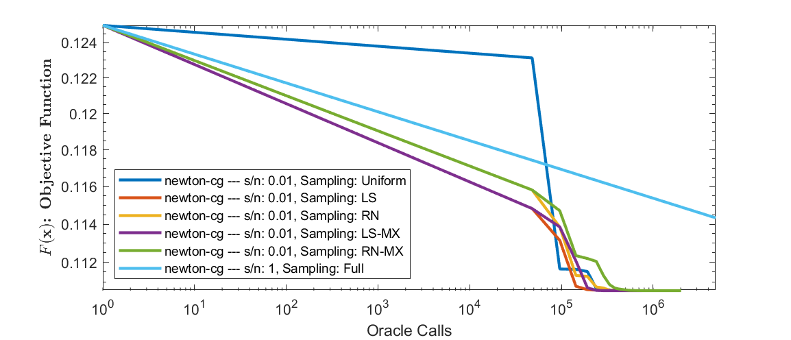
(a) $F(x_{k})$ vs. Oracle calls (Drive Diagnostics)

(b) $F(x_{k})$ vs. Oracle calls (Cover Type)

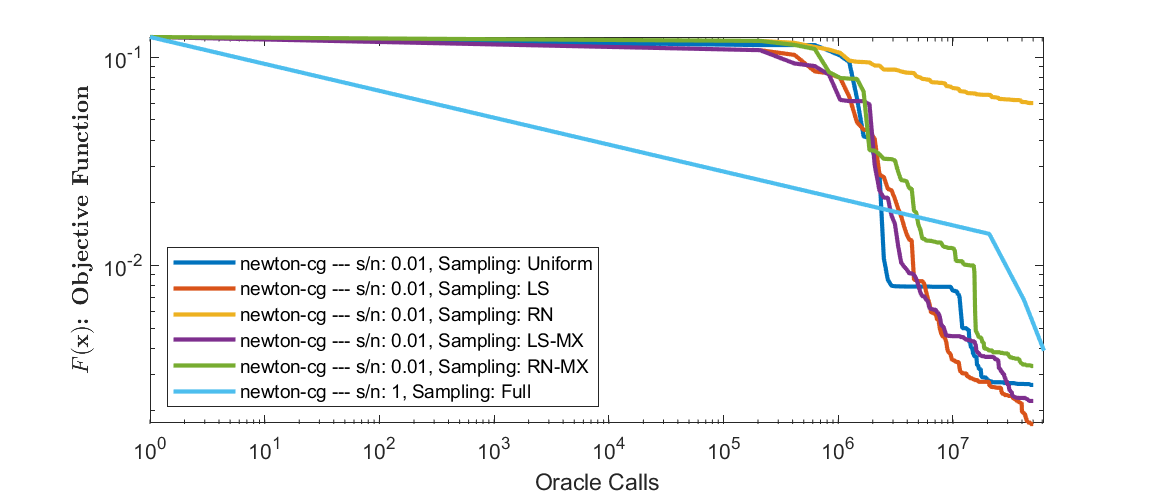
(c) $F(x_{k})$ vs. Oracle calls (UJIIndoorLoc)

Figure 4: Comparison of Newton-CG (Algorithm 5) using various sampling schemes.

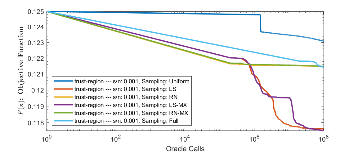
(a) $F(x_{k})$ vs. Oracle calls (Drive Diagnostics)

(b) $F(x_{k})$ vs. Oracle calls (Cover Type)

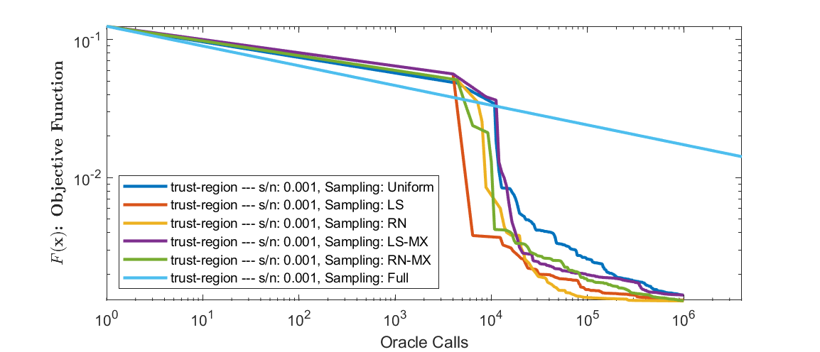
(c) $F(x_{k})$ vs. Oracle calls (UJIIndoorLoc)

Figure 5: Comparison of Trust-region (Algorithm 7) using various sampling schemes.

C.2 Evaluation of Hybrid Sketching Techniques

Here, to verify the result of Theorem 3, we evaluate the performance of Algorithm 7 by varying the terms involved in ${\mathbf{E}}$. We do this for a simple splitting of ${\mathbf{H}}={\mathbf{E}}+{\mathbf{N}}$, i.e., $T=1$ in Theorem 3. We fix the overall sample size and change the fraction of samples that are deterministically picked in ${\mathbf{E}}$. The results are depicted in Figure 6. The value in brackets in front of LS-Det is the fraction of samples that are included in ${\mathbf{E}}$, i.e., deterministic samples. “LS-Det (0)” and “LS-Det (1)” correspond to ${\mathbf{E}}=\bm{0}$ and ${\mathbf{N}}=\bm{0}$, respectively. The latter strategy has been used in low rank matrix approximations McCurdy [2018]. As it can be seen, the hybrid sampling approach is always competitive with, and at times significantly better than, LS-Det (0). As expected, LS-Det (1), which amounts to entirely deterministic samples, consistently performs worse. This can be easily attributed to the high bias of such a deterministic estimator.

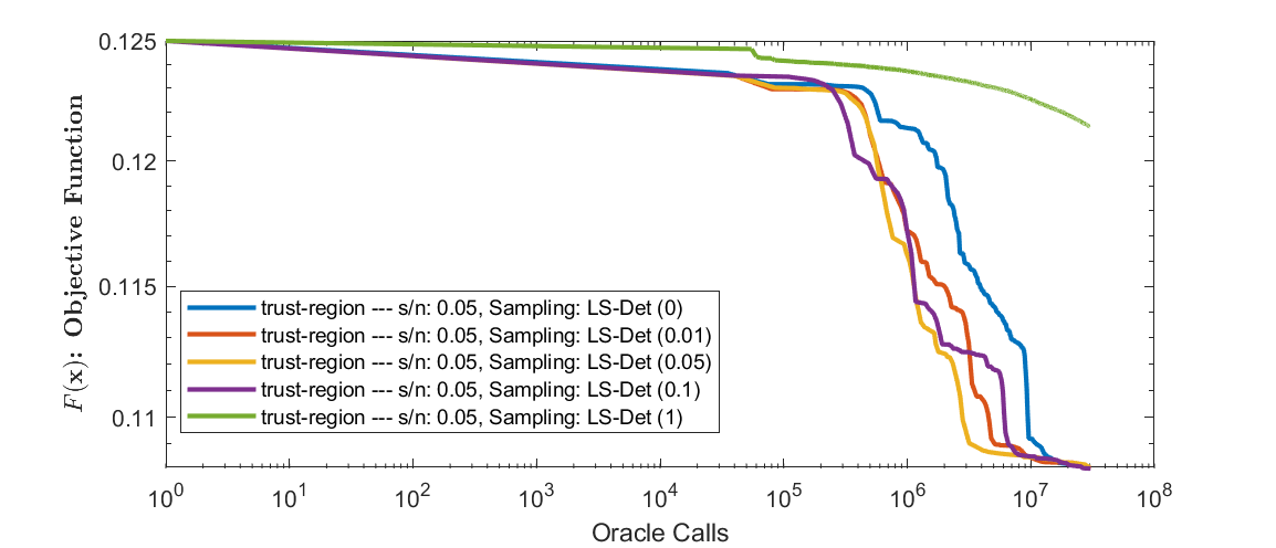
(a) $F(x_{k})$ vs. Oracle calls (Drive Diagnostics)

(b) $F(x_{k})$ vs. Oracle calls (Cover Type)

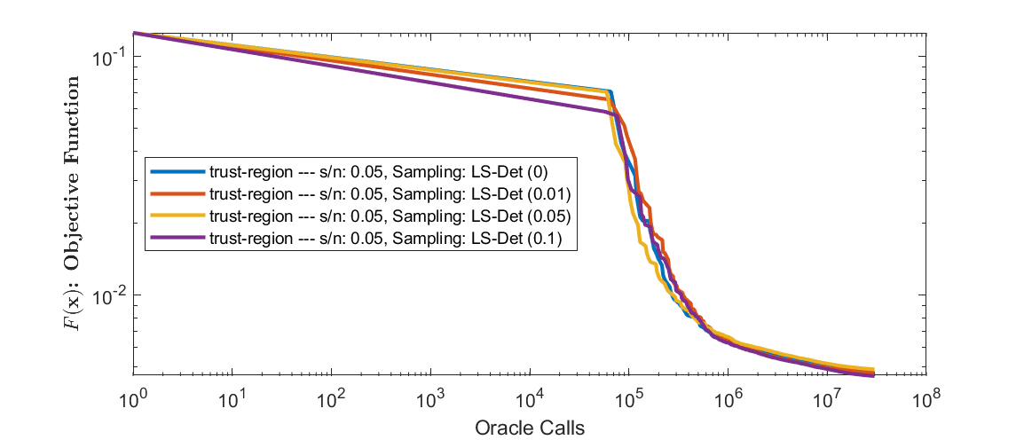
(c) $F(x_{k})$ vs. Oracle calls (UJIIndoorLoc)

Figure 6: Comparison of Algorithm 7 using hybrid randomized-deterministic sampling schemes. For all runs, the overall sample/mini-batch size for estimating the Hessian matrix is $s=0.05n$. The values in parentheses in front of LS-Det is the fraction of samples that are taken deterministically and included in ${\mathbf{E}}$.

References

- Andoni et al. [2016] Alexandr Andoni, Jiecao Chen, Robert Krauthgamer, Bo Qin, David P Woodruff, and Qin Zhang. On sketching quadratic forms. In Proceedings of the 2016 ACM Conference on Innovations in Theoretical Computer Science, pages 311–319, 2016.
- Beaton and Tukey [1974] Albert E Beaton and John W Tukey. The fitting of power series, meaning polynomials, illustrated on band-spectroscopic data. Technometrics, 16(2):147–185, 1974.
- Bollapragada et al. [2019] Raghu Bollapragada, Richard H Byrd, and Jorge Nocedal. Exact and inexact subsampled newton methods for optimization. IMA Journal of Numerical Analysis, 39(2):545–578, 2019.
- Chen et al. [2016] Yongxin Chen, Sei Zhen Khong, and Tryphon T Georgiou. On the definiteness of graph laplacians with negative weights: Geometrical and passivity-based approaches. In 2016 American Control Conference (ACC), pages 2488–2493. IEEE, 2016.
- Choi et al. [2011] Sou-Cheng T Choi, Christopher C Paige, and Michael A Saunders. MINRES-QLP: A Krylov subspace method for indefinite or singular symmetric systems. SIAM Journal on Scientific Computing, 33(4):1810–1836, 2011.
- Clarkson [2005] Kenneth L Clarkson. Subgradient and sampling algorithms for l 1 regression. In Proceedings of the sixteenth annual ACM-SIAM symposium on Discrete algorithms, pages 257–266. Society for Industrial and Applied Mathematics, 2005.
- Clarkson and Woodruff [2017] Kenneth L Clarkson and David P Woodruff. Low-rank approximation and regression in input sparsity time. Journal of the ACM (JACM), 63(6):1–45, 2017.
- Clarkson et al. [2016] Kenneth L Clarkson, Petros Drineas, Malik Magdon-Ismail, Michael W Mahoney, Xiangrui Meng, and David P Woodruff. The fast cauchy transform and faster robust linear regression. SIAM Journal on Computing, 45(3):763–810, 2016.
- Cohen et al. [2015a] Michael B Cohen, Yin Tat Lee, Cameron Musco, Christopher Musco, Richard Peng, and Aaron Sidford. Uniform sampling for matrix approximation. In Proceedings of the 2015 Conference on Innovations in Theoretical Computer Science, pages 181–190, 2015a.
- Cohen et al. [2015b] Michael B Cohen, Jelani Nelson, and David P Woodruff. Optimal approximate matrix product in terms of stable rank. arXiv preprint arXiv:1507.02268, 2015b.
- Cohen et al. [2017] Michael B Cohen, Cameron Musco, and Christopher Musco. Input sparsity time low-rank approximation via ridge leverage score sampling. In Proceedings of the Twenty-Eighth Annual ACM-SIAM Symposium on Discrete Algorithms, pages 1758–1777. SIAM, 2017.
- Cohen et al. [2019] Michael B Cohen, Yin Tat Lee, and Zhao Song. Solving linear programs in the current matrix multiplication time. In Proceedings of the 51st annual ACM SIGACT symposium on theory of computing, pages 938–942, 2019.
- Conn et al. [2000] Andrew R Conn, Nicholas IM Gould, and Philippe L Toint. Trust region methods. SIAM, 2000.
- Dasgupta et al. [2009] Anirban Dasgupta, Petros Drineas, Boulos Harb, Ravi Kumar, and Michael W Mahoney. Sampling algorithms and coresets for ell_p regression. SIAM Journal on Computing, 38(5):2060–2078, 2009.
- Drineas and Mahoney [2016] Petros Drineas and Michael W Mahoney. RandNLA: Randomized Numerical Linear Algebra. Communications of the ACM, 59(6):80–90, 2016.
- Dua and Graff [2017] Dheeru Dua and Casey Graff. UCI machine learning repository, 2017. URL http://archive.ics.uci.edu/ml.
- Erdogdu and Montanari [2015] Murat A Erdogdu and Andrea Montanari. Convergence rates of sub-sampled Newton methods. In Proceedings of the 28th International Conference on Neural Information Processing Systems-Volume 2, pages 3052–3060, 2015.
- Gould et al. [1999] Nicholas IM Gould, Stefano Lucidi, Massimo Roma, and Philippe L Toint. Solving the trust-region subproblem using the Lanczos method. SIAM Journal on Optimization, 9(2):504–525, 1999.
- Gross and Nesme [2010] David Gross and Vincent Nesme. Note on sampling without replacing from a finite collection of matrices. arXiv preprint arXiv:1001.2738, 2010.
- Indyk [2001] Piotr Indyk. Algorithmic applications of low-distortion geometric embeddings. In Proceedings 42nd IEEE Symposium on Foundations of Computer Science, pages 10–33. IEEE, 2001.
- Krahmer and Ward [2011] Felix Krahmer and Rachel Ward. New and improved johnson–lindenstrauss embeddings via the restricted isometry property. SIAM Journal on Mathematical Analysis, 43(3):1269–1281, 2011.
- Lenders et al. [2016] Felix Lenders, Christian Kirches, and Andreas Potschka. trlib: A vector-free implementation of the gltr method for iterative solution of the trust region problem. arXiv preprint arXiv:1611.04718, 2016.
- Liu et al. [2017] Xuanqing Liu, Cho-Jui Hsieh, Jason D Lee, and Yuekai Sun. An inexact subsampled proximal Newton-type method for large-scale machine learning. arXiv preprint arXiv:1708.08552, 2017.
- Liu and Roosta [2019] Yang Liu and Fred Roosta. Stability Analysis of Newton-MR Under Hessian Perturbations. arXiv preprint arXiv:1909.06224, 2019.
- Mahoney [2011] Michael W Mahoney. Randomized algorithms for matrices and data. Foundations and Trends® in Machine Learning, 3(2):123–224, 2011.
- McCurdy [2018] Shannon McCurdy. Ridge regression and provable deterministic ridge leverage score sampling. In Advances in Neural Information Processing Systems, pages 2463–2472, 2018.
- Meng and Mahoney [2013] Xiangrui Meng and Michael W Mahoney. Low-distortion subspace embeddings in input-sparsity time and applications to robust linear regression. In Proceedings of the forty-fifth annual ACM symposium on Theory of computing, pages 91–100, 2013.
- Nocedal and Wright [2006] Jorge Nocedal and Stephen Wright. Numerical optimization. Springer Science & Business Media, 2006.
- Paouris et al. [2017] Grigoris Paouris, Petros Valettas, and Joel Zinn. Random version of dvoretzky’s theorem in . Stochastic Processes and their Applications, 127(10):3187–3227, 2017.
- Pham and Pagh [2013] Ninh Pham and Rasmus Pagh. Fast and scalable polynomial kernels via explicit feature maps. In Proceedings of the 19th ACM SIGKDD international conference on Knowledge discovery and data mining, pages 239–247, 2013.
- Pilanci and Wainwright [2017] Mert Pilanci and Martin J Wainwright. Newton sketch: A near linear-time optimization algorithm with linear-quadratic convergence. SIAM Journal on Optimization, 27(1):205–245, 2017.
- Rashtchian et al. [2020] Cyrus Rashtchian, David P Woodruff, and Hanlin Zhu. Vector-matrix-vector queries for solving linear algebra, statistics, and graph problems. arXiv preprint arXiv:2006.14015, 2020.
- Roosta and Mahoney [2019] Farbod Roosta and Michael W Mahoney. Sub-sampled Newton methods. Mathematical Programming, 174(1-2):293–326, 2019.
- Roosta et al. [2018] Farbod Roosta, Yang Liu, Peng Xu, and Michael W Mahoney. Newton-MR: Newton’s Method Without Smoothness or Convexity. arXiv preprint arXiv:1810.00303, 2018.
- Saad [2003] Yousef Saad. Iterative methods for sparse linear systems, volume 82. SIAM, 2003.
- Shalev-Shwartz and Ben-David [2014] Shai Shalev-Shwartz and Shai Ben-David. Understanding machine learning: From theory to algorithms. Cambridge university press, 2014.
- Sohler and Woodruff [2011] Christian Sohler and David P Woodruff. Subspace embeddings for the l1-norm with applications. In Proceedings of the forty-third annual ACM symposium on Theory of computing, pages 755–764, 2011.
- Sorensen [1982] Danny C Sorensen. Newton’s method with a model trust region modification. SIAM Journal on Numerical Analysis, 19(2):409–426, 1982.
- Steihaug [1983] Trond Steihaug. The conjugate gradient method and trust regions in large scale optimization. SIAM Journal on Numerical Analysis, 20(3):626–637, 1983.
- Toint [1981] Philippe L Toint. Towards an efficient sparsity exploiting Newton method for minimization. Sparse matrices and their uses, page 1981, 1981.
- Tripuraneni et al. [2018] Nilesh Tripuraneni, Mitchell Stern, Chi Jin, Jeffrey Regier, and Michael I Jordan. Stochastic cubic regularization for fast nonconvex optimization. In Advances in neural information processing systems, pages 2899–2908, 2018.
- Tropp et al. [2015] Joel A Tropp et al. An introduction to matrix concentration inequalities. Foundations and Trends® in Machine Learning, 8(1-2):1–230, 2015.
- Wang and Woodruff [2019] Ruosong Wang and David P Woodruff. Tight bounds for oblivious subspace embeddings. In Proceedings of the Thirtieth Annual ACM-SIAM Symposium on Discrete Algorithms, pages 1825–1843. SIAM, 2019.
- Woodruff and Zhang [2013] David Woodruff and Qin Zhang. Subspace embeddings andell_p-regression using exponential random variables. In Conference on Learning Theory, pages 546–567, 2013.
- Woodruff et al. [2014] David P Woodruff et al. Sketching as a tool for numerical linear algebra. Foundations and Trends® in Theoretical Computer Science, 10(1–2):1–157, 2014.
- Xu et al. [2016] Peng Xu, Jiyan Yang, Farbod Roosta, Christopher Ré, and Michael W Mahoney. Sub-sampled newton methods with non-uniform sampling. In Advances in Neural Information Processing Systems, pages 3000–3008, 2016.
- Xu et al. [2019] Peng Xu, Farbod Roosta, and Michael W Mahoney. Newton-type methods for non-convex optimization under inexact Hessian information. Mathematical Programming, 2019. doi:10.1007/s10107-019-01405-z.
- Xu et al. [2020] Peng Xu, Farbod Roosta, and Michael W. Mahoney. Second-Order Optimization for Non-Convex Machine Learning: An Empirical Study. In Proceedings of the 2020 SIAM International Conference on Data Mining. SIAM, 2020.
- Yao et al. [2018] Zhewei Yao, Peng Xu, Farbod Roosta, and Michael W Mahoney. Inexact non-convex Newton-type methods. arXiv preprint arXiv:1802.06925, 2018. Under review.