Sharp convergence to steady states of Allen-Cahn

Abstract.

In our recent work we found a surprising breakdown of symmetry conservation: using standard numerical discretization with very high precision the computed numerical solutions corresponding to very nice initial data may converge to completely incorrect steady states due to the gradual accumulation of machine round-off error. We solved this issue by introducing a new Fourier filter technique for solutions with certain band gap properties. To further investigate the attracting basin of steady states we classify in this work all possible bounded nontrivial steady states for the Allen-Cahn equation. We characterize sharp dependence of nontrivial steady states on the diffusion coefficient and prove strict monotonicity of the associated energy. In particular, we establish a certain self-replicating property amongst the hierarchy of steady states and give a full classification of their energies and profiles. We develop a new modulation theory and prove sharp convergence to the steady state with explicit rates and profiles.

1. Introduction

In this paper, we consider the following one-dimensional Allen-Cahn equation posed on the periodic torus $\mathbb{T}=[-\pi,\pi]$:

$$\begin{cases}\partial_{t}u=\kappa^{2}\partial_{xx}u-f(u),\\ u\bigr{|}_{t=0}=u_{0},\end{cases}$$ (1.1)

where $\kappa>0$ measures the strength of diffusion, $f(u)=u^{3}-u=F^{\prime}(u)$, and $F(u)=(u^{2}-1)^{2}/4$ is the usual double-well potential. The function $u:\mathbb{T}\to\mathbb{R}$ represents the concentration difference of phases in an alloy and typically has values in the physical range $[-1,1]$.

In our concurrent work [18], we find a very surprising breakdown of parity in typical high-precision computation of (1.1) with very smooth initial data. For example take $\kappa=1$ and consider the equation (1.1) with the initial data $u_{0}(x)$ being an odd function of $x$ such as $u_{0}(x)=\sin x$. By simple PDE arguments the smooth solution should preserve the odd symmetry for all time. However numerical discretized solutions turn out to fail to conserve this parity and converge quickly to the spurious states $u=\pm 1$ in not very long time simulations. This striking contradiction is a manifestation of the gradual accumulation of non-negligible machine round off errors over time. To resolve this issue, we introduced a new Fourier filter method which works successfully for a class of initial data with certain symmetry and band-gap properties. By eliminating the unwanted projections into the unstable directions at each iteration, we rigorously show that the filtered solution will converge to the true steady state in long time simulations.

A natural next task is to understand the situation for general solutions without symmetries or band-gap properties. The pivotal step is to categorize the steady states of the elliptic Allen-Cahn equations and analyze in detail their spectral properties. For full generality we shall consider the steady states of (1.1) on the whole real axis, i.e.

$$\kappa^{2}u^{\prime\prime}+u-u^{3}=0\quad\mathrm{in}\quad\mathbb{R}.$$ (1.2)

In [9] De Giorgi raised the problem about proving that bounded solutions to $\Delta u=F^{\prime}(u)$ in dimensions $2\leq n\leq 8$ which are monotone in one direction, must depend only on one variable in dimension. Since then there are many works in understanding the structure of the solutions. Particularly, in dimension $n=2$ and $n=3$, Ghoussoub-Gui [14] and Ambrosio-Cabré [2] proved the conjecture respectively. Savin [22] proved the De Giorgi conjecture up to dimension 8 under some additional assumption. The same conclusion has been obtained by Wang [26] with a different method. In [10] Del Pino-Kowalczyk-Wei established the existence of a counterexample in dimensions $n\geq 9$. We refer the readers to [1] for background on De Giorgi’s conjecture, [6, 7] for the study on the symmetry properties of the solutions to the fractional Allen-Cahn equation and the recent survey [11] for some related open problems. It is known that the monotone solutions to (1.2) in any dimension are stable solutions, i.e., the second variation of the associated energy is non-negative, where the energy functional is defined as

$$E(u)=\int_{\mathbb{R}}\left(\frac{\kappa^{2}}{2}|\nabla u|^{2}+\frac{1}{4}(1-u^{2})^{2}\right)dx.$$ (1.3)

Recently, there is a new counterpart problem for the stable solutions to Allen-Cahn equation (see e.g. [22, 21, 19] and references therein). Based on the monotonicity assumption it is natural to consider the two sides limit (without loss of generality we assume the function is monotone in $x_{n}$)

$$u^{+}:=\lim_{x_{n}\to+\infty}u,\quad u^{-}:=\lim_{x_{n}\to-\infty}u.$$ (1.4)

It is known that the limit functions only depend on the previous $n-1$ variables. Savin [22] has proved if $u^{\pm}$ are $1-$D, then the original $u$ is also $1-$D. From a general perspective it is of some importance to study the stable solutions and its energy functional (1.3) in order to understand the structure of steady states. In the first part of this paper, we shall classify all the steady states of the $2\pi$-periodic solutions to (1.2). Furthermore we consider the variation on the energy of the ground state with respect to $\kappa$.

Theorem 1.1.

Let $0<\kappa<1$ and $m_{\kappa}$ be the largest positive integer such that $m_{\kappa}\kappa<1$, then equation (1.2) admits exactly $m_{\kappa}$ non-constant $2\pi$ periodic solutions up to some translation and odd reflection.

It is known that any periodic solution of (1.2) is bounded. By Modica’s estimate one can get that $|u|\leq 1$, see [20]. For convenience of the readers we shall include an elementary proof for the one dimensional case, see Proposition 2.4. By using Proposition 2.4 it suffices for us to consider periodic solutions to (1.2) satisfying $|u|<1$, since $u\equiv 1$ or $u\equiv-1$ provides the trivial global minimizers of (1.2) from an energy perspective.

To state the next result, we define the energy for $2\pi$-periodic functions $u\in H^{1}(\mathbb{T})$:

$$E_{\kappa}(u)=\int_{\mathbb{T}}\left(\frac{\kappa^{2}}{2}|\partial_{x}u|^{2}+\frac{1}{4}(1-u^{2})^{2}\right)dx.$$ (1.5)

Define

$$E_{\kappa}=\inf_{u\in\mathcal{S}}E_{\kappa}(u),$$ (1.6)

where

$$\mathcal{S}=\{\phi~{}|~{}\phi(x)\in H^{1}(\mathbb{T})~{}\mbox{solves}~{}\eqref{1.eac},~{}\phi(x)=\phi(x+2\pi)~{}\mathrm{and}~{}|\phi|<1,~{}x\in\mathbb{R}\}.$$ (1.7)

For the $2\pi$-periodic solutions of (1.2), we call $u$ a ground state if $u$ is the least energy solution. For fixed $0<\kappa<1$, by using the classification result in Proposition 2.4, we can prove that the ground state solution is unique up to a translation and reflection. To fix the symmetries it is convenient to introduce the notion of odd zero-up ground states (see Definition 3.2). In particular if a ground state solution $u$ is odd and satisfy $u^{\prime}(0)>0$, we shall call it an odd zero-up ground state and denote it by $U_{\kappa}$. For any $0<\kappa<1$, define $m_{\kappa}\geq 1$ as the unique integer such that

$$\frac{1}{m_{\kappa}+1}\leq\kappa<\frac{1}{m_{\kappa}}.$$ (1.8)

For each $j=1,\cdots,m_{\kappa}$, define (note below that $j\kappa<1$)

$$\tilde{u}_{\kappa,j}(x)=U_{j\kappa}(jx).$$ (1.9)

Then $\{\tilde{u}_{\kappa,j}\}_{j=1}^{m_{\kappa}}$ are all the possible odd zero-up solutions to (3.1). Furthermore the energies of $\tilde{u}_{\kappa,j}$ are given by

$$E_{\kappa}(\tilde{u}_{\kappa,j}) =\int_{\mathbb{T}}\Bigl{(}\frac{1}{2}(\kappa\partial_{x}{\tilde{u}_{\kappa,j}})^{2}+\frac{1}{4}(\tilde{u}_{\kappa,j}^{2}-1)^{2}\Bigr{)}dx=E_{j\kappa}(U_{j\kappa}).$$ (1.10)

With this notation, we now state the following structure theorem on the energy functional $E_{\kappa}(u)$ of the $2\pi$-periodic solutions.

Theorem 1.2.

Let $E_{\kappa}$ be defined in (1.6). Then it can be achieved for any $\kappa>0.$ In addition, we have

• $E_{\kappa}=\frac{\pi}{2}$ for $\kappa\geq 1$ and it is only achieved by the zero function;

• $E_{\kappa}$ is achieved by $U_{\kappa}$ whenever $\kappa\in(0,1)$;

• If $0<\kappa_{1}<\kappa_{2}\leq 1$, then there is strict monotonicity $E_{\kappa_{1}}<E_{\kappa_{2}}$;

• The odd zero-up ground state $U_{\kappa}$ satisfies

  $$\left|U_{\kappa}(x)-\tanh\left(\frac{x}{\sqrt{2}\kappa}\right)\right|\leq C\exp\left(-\frac{d}{\kappa}\right),$$ (1.11)

  for some universal positive constants $C$ and $d$, and

  $$\lim\limits_{\kappa\to 0}\frac{E_{\kappa}}{{\kappa}}=\frac{4}{3}\sqrt{2}>0.$$ (1.12)

• For $0<\kappa<1$, the $2\pi$-periodic solutions of problem 1.2 have the following replica property: any $2\pi$-periodic solution $u$ of (1.2) which is not identically $\pm 1$ or $0$ must coincide (after some shift and odd reflection if necessary) with $\tilde{u}_{\kappa,j}$ for some integer $j<1/\kappa$. Here $\tilde{u}_{\kappa,j}$ is defined in (1.9). Furthermore $E_{\kappa}(u)=E_{m\kappa}(U_{m\kappa}).$

From Theorem 1.1 we can see that $0$ is the only $2\pi$-periodic solution to equation (1.2) whenever $\kappa\geq 1$. This is in complete accord with numerical experiments. Furthermore when $\kappa>1$, $u(x,t)$ converges to $0$ exponentially as $O(e^{-(\kappa^{2}-1)t})$, while the convergence rate becomes $O(t^{-\frac{1}{2}})$ for $\kappa=1$. In the second part of this work, we shall rigorously prove these convergence results and identify the explicit profiles. Our strategy is quite robust and we shall illustrate it for a general fractional Allen-Cahn equation

$$\begin{cases}\partial_{t}u=-\kappa^{2}\Lambda^{\gamma}u+u-u^{3},\quad(x,t)\in\mathbb{T}\times(0,\infty),\\ u\bigr{|}_{t=0}=u_{0},\end{cases}$$ (1.13)

where $\Lambda^{\gamma}=(-\partial_{xx})^{\frac{\gamma}{2}}$ is the fractional Laplacian of order $\gamma\in(0,2].$ When $\gamma=2$ it coincides with the usual $-\partial_{xx}.$ For simplicity of presentation we state below a simple version of the obtained results in Section 4. Sharper results concerning profiles, rates etc can be found in Section 4.

Theorem 1.3 (Vanishing as $t\to\infty$).

Let $\kappa\geq 1$ and $0<\gamma\leq 2$. Assume $u_{0}$ is $2\pi$ periodic, odd and bounded. Suppose $u$ is the solution to (1.13) corresponding to the initial data $u_{0}$. If $\kappa>1$, we have

$$u(x,t)=e^{-(\kappa^{2}-1)t}\alpha_{*}\sin x+r(t),\qquad\forall\,t\geq 1,$$ (1.14)

where $\alpha_{*}$ depends on $u_{0},\gamma$ and $\kappa,$ and $\|r(t)\|_{H^{10}(\mathbb{T})}=o(e^{-(\kappa^{2}-1)t})$ as $t\to+\infty$.

For $\kappa=1$, we have

$$u(x,t)=t^{-\frac{1}{2}}\beta_{*}\sin x+r_{1}(t),\qquad\forall\,t\geq 1,$$ (1.15)

where $\beta_{*}$ depends on $u_{0},\gamma$ and $\|r_{1}(t)\|_{H^{10}(\mathbb{T})}=o(t^{-\frac{1}{2}})$ as $t\to+\infty$.

When $\kappa\in(0,1)$, the corresponding theory of convergence becomes quite involved. Indeed, from Theorem 1.1 we see that the number of steady states (up to identification of symmetry) increases as $O(1/\kappa)$ when $\kappa$ decays to zero. At the moment there is no general theory for the precise identification of the corresponding steady for arbitrary initial data. However for a class of benign initial data, we have the following precise and definite convergence results.

Theorem 1.4.

Let $0<\kappa<1$. Assume the initial data $u_{0}:\mathbb{R}\to\mathbb{R}$ is $2\pi$-periodic, odd and non-negative in $[0,\pi],$ then we have $u(x,t)\to U_{\kappa}$ or $0$ as $t\to\infty$. Moreover, if $u_{0}\neq 0$ and and $E_{\kappa}(u_{0})\leq\frac{\pi}{2}$, then $u(x,t)\to U_{\kappa}$ as $t\to\infty$ and the rate of convergence is exponential in time.

To our best knowledge Theorem 1.4 along with earlier results are the first sharp quantitative convergence results on the Allen-Cahn equation. We plan to develop this program on much more general phase field models in forthcoming works.

The rest of this paper is organized as follows. In Section 2 we introduce preliminary analysis of the steady states and examine in detail the profiles of the ground states. In Section 3 we prove Theorems 1.1 and 1.2, give full classification of the steady states and analyze their profiles and energy monotonicity. In Section 4 we study the convergence of the general parabolic Allen-Cahn equation (1.13), and prove Theorems 1.3 and 1.4. In Section 5 we give concluding remarks. The proof of Proposition 2.2 is given in the appendix.

2. Classification of steady states

The solutions to $\kappa^{2}u^{\prime\prime}+u-u^{3}=0$ are remarkably rigid, as documented by the following “patching” of nonlinear solutions.

Proposition 2.1 (Patching of nonlinear solutions via reflection).

The following hold.

• Even reflection. Suppose $\kappa>0$, and for some $\epsilon_{0}>0$ we have

  $$\kappa^{2}u^{\prime\prime}+u-u^{3}=0,\qquad\forall\,-\epsilon_{0}<x<0,$$ (2.1)

  where $u\in C^{2}((-\epsilon_{0},0))$ and we assume $\lim\limits_{x\to 0-}u^{\prime}(x)=0$. Define $u(x)=u(-x)$ for $0<x<\epsilon_{0}$. Then it holds that $u\in C^{\infty}((-\epsilon_{0},\epsilon_{0}))$ with $u^{\prime}(0)=0$ and solving the same equation on the whole interval.

• Odd reflection. Suppose $\kappa>0$, and for some $\epsilon_{0}>0$ we have

  $$\kappa^{2}u^{\prime\prime}+u-u^{3}=0,\qquad\forall\,0<x<\epsilon_{0}.$$ (2.2)

  where $u\in C^{2}((0,\epsilon_{0}))$ and we assume $\lim\limits_{x\to 0+}u(x)=0$. Define $u(x)=-u(-x)$ for $-\epsilon_{0}<x<0$. Then it holds that $u\in C^{\infty}((-\epsilon_{0},\epsilon_{0}))$ with $u(0)=0$ and solving the same equation on the whole interval.

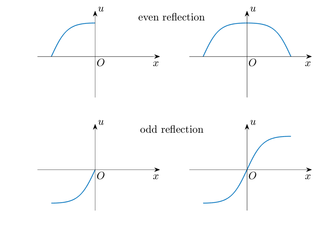
Figure 1. Even reflection and odd reflection.

Remark 2.2.

Proposition 2.1 shows that the solution is remarkably rigid. If we know the profile of $u$ on some interval $(a,b)$ with $u(a)=0,~{}u^{\prime}(b)=0$. Then the solution can be uniquely determined on a larger interval.

Proof.

We shall only prove the first case as the second case is similar. First it is not difficult to that $u$ has bounded derivatives in $[-\epsilon_{0}/2,0)$ which can be extended to $0$ from the left. The extended $u$ satisfies the equation on $(-\epsilon_{0},0)\cap(0,\epsilon_{0})$. Furthermore the equation also holds at $x=0$ up to third order derivatives. Then we can bootstrap the regularity of $u$ by using the equation and conclude that $u\in C^{\infty}$. ∎

Observe that for $u_{0}(x)=\sin x$, since $f(u)=u^{3}-u$, we have

$$u(x,t)=\sum_{\text{$m\geq 1$: {$m$ is odd}}}c_{m}(t)\sin mx.$$ (2.3)

In particular it follows that the corresponding steady state $u_{\infty}$ is odd. If $2\pi$ is the minimal period (such solution is actually the odd zero-up ground state up to a reflection if necessary, see Definition 3.2), then $u_{\infty}(0)=u_{\infty}^{\prime}(\frac{\pi}{2})=0.$ In addition, $u_{\infty}$ satisfies the steady state equation

$$\kappa^{2}u^{\prime\prime}-f(u)=0\quad\mbox{on}\quad\mathbb{T}.$$ (2.4)

We may look for the steady state such that it is monotonically increasing on $[0,\frac{\pi}{2}]$ with $u_{\infty}(0)=u_{\infty}^{\prime}(\frac{\pi}{2})=0$. Effectively by using reflection symmetry, the whole graph of $u_{\infty}$ will be determined by its graph on the interval $[0,\frac{\pi}{2}]$.

To simplify the notation we now write $u=u_{\infty}$ as the desired steady state. We consider the regime $0<\kappa<1$ (for simplicity we suppress the notational dependence of $u$ on $\kappa$). Denote $u(\frac{\pi}{2})=N<1$ and observe that we should have $N\to 1$ as $\kappa\to 0$. Multiplying $\eqref{2.steady}$ by $u^{\prime}$ and using $u^{\prime}(\frac{\pi}{2})=0$, we have

$$(u^{\prime})^{2}=\frac{1}{2{\kappa^{2}}}((u^{2}-1)^{2}-(N^{2}-1)^{2}).$$ (2.5)

If $u$ is monotonically increasing, it satisfies

$$u^{\prime}(x)=\frac{1}{\sqrt{2}{\kappa}}\sqrt{(u^{2}-1)^{2}-(N^{2}-1)^{2}},$$ (2.6)

with $u(0)=0$, $u(\frac{\pi}{2})=N$. We then obtain

$$\int_{0}^{N}\frac{1}{\sqrt{(u^{2}-1)^{2}-(1-N^{2})^{2}}}du=\frac{\pi}{2\sqrt{2}\kappa}.$$ (2.7)

For each fixed $0<\kappa<1$, there exists a unique $0<N=N(\kappa)<1$ such that the above identity holds. Furthermore one can determine the dependence of $N$ on $\kappa$. Indeed by a change of variable $u\to N\sin\theta$, the left-hand side of the above equation is denoted by

$$g(N) :=\int_{0}^{N}\frac{1}{\sqrt{(u^{2}-1)^{2}-(1-N^{2})^{2}}}du=\int_{0}^{\frac{\pi}{2}}\frac{1}{\sqrt{2-N^{2}(1+\sin^{2}\theta)}}d\theta.$$ (2.8)

Here we note that $g$ is monotonically increasing on $[0,1)$, $g(0)=\frac{\pi}{2\sqrt{2}}$ and $g(1)=\infty$. In particular we see the necessity of $\kappa<1$! Otherwise if $\kappa\geq 1$, the equation (2.4) admits the trivial solution $u\equiv 0$. For $0<\kappa\ll 1$, it is not difficult to check that

$$1-N(\kappa)=O(e^{-\frac{c}{\kappa}}).$$ (2.9)

Sharper asymptotics can certainly be derived.

We summarize the above discussion as the following proposition.

Proposition 2.3 (Characterization of a special steady state for $0<\kappa<1$).

The following hold:

1. The function $g$ defined in (2.8) is monotonically increasing on $[0,1)$, $g(0)=\frac{\pi}{2\sqrt{2}}$ and $g(N)\to\infty$ as $N\to 1$.

2. For any $0<\kappa<1$, there exists a unique $0<N_{\kappa}<1$ such that

   $$g(N_{\kappa})=\frac{\pi}{2\sqrt{2}\kappa}.$$ (2.10)

   Furthermore we have

   $$c_{1}e^{-\frac{c_{2}}{\kappa}}<1-N_{\kappa}<c_{3}e^{-\frac{c_{4}}{\kappa}},$$ (2.11)

   where $c_{i}>0$, $i=1,\cdots,4$ are absolute constants.

3. For any $0<\kappa<1$, there exists a $2\pi$-periodic $C^{\infty}$ odd function $u_{\kappa}$ such that

   • $u_{\kappa}$ is a steady state, i.e. $\kappa^{2}u_{\kappa}^{\prime\prime}-f(u_{\kappa})=0$.

   • $u_{\kappa}(0)=u_{\kappa}^{\prime}(\frac{\pi}{2})=0$, $u_{\kappa}(\frac{\pi}{2})=N_{\kappa}$, and $u_{\kappa}$ is monotonically increasing on $[0,\frac{\pi}{2}]$.

   • $u_{\kappa}(\pi-x)=u_{\kappa}(x)$ for $\frac{\pi}{2}\leq x\leq\pi$.

   Moreover for $0<\kappa\ll 1$, we have

   $$0\leq\tanh\left(\frac{x}{\sqrt{2}\kappa}\right)-u_{\kappa}(x)\leq\exp(-\frac{c_{5}}{\kappa}),\qquad\forall\,0\leq x\leq\frac{\pi}{2},$$ (2.12)

   where $c_{5}>0$ is an absolute constant.

Proof.

1. For fixed $N\in[0,1)$, taking the derivative of $g(N)$ with respect to $N$, we have

$$g^{\prime}(N)=\int_{0}^{\frac{\pi}{2}}\frac{N(1+\sin^{2}\theta)}{(2-N^{2}(1+\sin^{2}\theta))^{\frac{3}{2}}}d\theta.$$ (2.13)

It is not difficult to verify that both the numerator and denomenator are positive in $(0,\frac{\pi}{2})$, therefore, we have shown that $g^{\prime}(N)>0$ and it proves that $g$ is monotonically increasing for $N\in[0,1)$. When $N=0$, we have $g(0)=\int_{0}^{\frac{\pi}{2}}\frac{1}{\sqrt{2}}d\theta=\frac{\pi}{2\sqrt{2}}$. While as $N$ is close to $1$, we have

$$g(N) =\int_{0}^{\frac{\pi}{2}}\frac{1}{\sqrt{2-2N^{2}+N^{2}\cos^{2}\theta}}d\theta=\int_{0}^{\frac{\pi}{2}}\frac{1}{\sqrt{2-2N^{2}+N^{2}\sin^{2}\theta}}d\theta$$ (2.14)

$$>\int_{0}^{1}\frac{1}{\sqrt{2-2N^{2}+N^{2}\theta^{2}}}d\theta>\frac{1}{N}\int_{\delta}^{1}\frac{1}{\sqrt{\delta^{2}+\theta^{2}}}d\theta$$

$$>\frac{1}{N}\int_{\delta}^{1}\frac{1}{\sqrt{2}\theta}d\theta=-\frac{1}{\sqrt{2}N}\log\delta,$$

where

$$\delta=\sqrt{\frac{2-2N^{2}}{N^{2}}}\to 0,\quad\mbox{as }N\to 1.$$ (2.15)

Here, it is assumed implicitly that $N>\sqrt{\frac{2}{3}}$ so that $\delta<1$. Then, it is easy to see that $g(N)\to\infty$ as $N\to 1$.

2. The existence and uniqueness of $N_{\kappa}$ follows easily from the behavior of the function $g(\cdot)$. Now we shall show the upper and lower bounds on $N_{\kappa}$. It is clear from Step 1 that $N_{\kappa}\to 1$ as $\kappa\to 0$. If $N_{\kappa}\leq\sqrt{\frac{2}{3}}$, then $\kappa$ is bounded away from zero by an absolute constant and the desired estimate (2.11) clearly holds in this case. Thus we only need to consider the situation $N_{\kappa}>\sqrt{\frac{2}{3}}$. To ease the notation we denote $N=N_{\kappa}$ with $N>\sqrt{\frac{2}{3}}$. From (2.14), we have

$$\frac{\pi}{2\sqrt{2}\kappa}=g(N)>-\frac{1}{\sqrt{2}N}\log\delta,$$ (2.16)

which yields directly

$$1-N>\frac{N^{2}}{2+2N}e^{-\frac{N\pi}{\kappa}}.$$ (2.17)

On the other hand, using $\sin\theta>\frac{2}{\pi}\theta$, we have

$$\frac{\pi}{2\sqrt{2}\kappa} =g(N)=\int_{0}^{\frac{\pi}{2}}\frac{1}{\sqrt{2-2N^{2}+N^{2}\sin^{2}\theta}}d\theta<\int_{0}^{\frac{\pi}{2}}\frac{1}{\sqrt{2-2N^{2}+N^{2}\left(\frac{2}{\pi}\theta\right)^{2}}}d\theta$$ (2.18)

$$=\int_{0}^{1}\frac{\pi}{2N\sqrt{\delta^{2}+\tilde{\theta}^{2}}}d\tilde{\theta}=\int_{0}^{\delta}\frac{\pi}{2N\sqrt{\delta^{2}+\tilde{\theta}^{2}}}d\tilde{\theta}+\int_{\delta}^{1}\frac{\pi}{2N\sqrt{\delta^{2}+\tilde{\theta}^{2}}}d\tilde{\theta}$$

$$<\frac{\pi}{2N}-\frac{\pi}{2\sqrt{2}N}\log\delta,$$

which yields

$$1-N<\frac{N^{2}}{2+2N}e^{2\sqrt{2}-\frac{2N}{\kappa}}.$$ (2.19)

Therefore, when $N>\sqrt{\frac{2}{3}}$, we have

$$\frac{1}{3+\sqrt{6}}e^{-\frac{\pi}{\kappa}}<\frac{N^{2}}{2+2N}e^{-\frac{N\pi}{\kappa}}<1-N<\frac{N^{2}}{2+2N}e^{2\sqrt{2}-\frac{2N}{\kappa}}<\frac{e^{2\sqrt{2}}}{4}e^{-\frac{2\sqrt{2}}{\sqrt{3}\kappa}}.$$ (2.20)

3. Fix $0<\kappa<1$ and consider the function

$$h(u)=\int_{0}^{u}\frac{\sqrt{2}{\kappa}}{\sqrt{(y^{2}-1)^{2}-(1-N^{2})^{2}}}dy,\quad 0\leq u\leq N.$$ (2.21)

Clearly $h:\,[0,N]\to[0,\frac{\pi}{2}]$ is strictly monotonically increasing and bijective. The inverse map of $h(u)$ then defines the desired function $u_{\kappa}$ on the interval $[0,\frac{\pi}{2}]$. It is known that $u(\frac{\pi}{2})=N$ and $u^{\prime}(\frac{\pi}{2})=0$, by Proposition 2.1 we derive that $u$ is even respect to $x=\frac{\pi}{2},$ i.e., $u(x)=u(\pi-x)$ for $x\in\left(0,\frac{\pi}{2}\right).$

Finally to show (2.12), we denote $\theta(x)=\tanh(\frac{x}{\sqrt{2}\kappa})$. Clearly

$$\left\{\begin{aligned} &\frac{du_{\kappa}}{dx}=\frac{1}{\sqrt{2}\kappa}\sqrt{(u^{2}_{\kappa}-1)^{2}-(N^{2}-1)^{2}},\\ &\frac{d\theta}{dx}=\frac{1}{\sqrt{2}\kappa}(1-\theta^{2}),\\ &u_{\kappa}(0)=\theta(0)=0,\end{aligned}\right.$$ (2.22)

Observe that

$$\frac{du_{\kappa}}{dx}<\frac{1}{\sqrt{2}\kappa}(1-u_{\kappa}^{2}).$$ (2.23)

Denote $\eta(x)=u_{\kappa}(x)-\theta(x)$. Clearly $\eta(0)=0$ and

$$\eta^{\prime}<-\frac{1}{\sqrt{2}\kappa}(u_{\kappa}+\theta)\eta.$$ (2.24)

This implies that $\eta(x)\leq 0$ for all $0\leq x\leq\frac{\pi}{2}$. Thus

$$u_{\kappa}(x)-\theta(x)\leq 0,\qquad\forall\,0\leq x\leq\frac{\pi}{2}.$$ (2.25)

We now show the lower bound. By (2.11) we can choose an absolute constant $\delta_{0}>0$ sufficiently small such that

$$1-N^{2}<c_{3}e^{-\frac{c_{4}}{\kappa}}<\frac{1}{100}(1-\theta(x)^{2}),\qquad\forall\,0\leq x\leq\delta_{0}.$$ (2.26)

This implies

$$\sqrt{(1-u_{\kappa}(x)^{2})^{2}-(1-N^{2})^{2}}+1-\theta(x)^{2}\geq C(1-u_{\kappa}(x)^{2}+1-\theta(x)^{2}),$$ (2.27)

for $x\in[0,\delta_{0}]$ and some generic constant $C>0$. Now observe that

$$\frac{d}{dx}\eta=\frac{1}{\sqrt{2}\kappa}\frac{(1-u_{\kappa}^{2})^{2}-(1-\theta^{2})^{2}-(1-N^{2})^{2}}{\sqrt{(1-u_{\kappa}^{2})^{2}-(1-N^{2})^{2}}+1-\theta^{2}}.$$ (2.28)

Thus for $0<x\leq\delta_{0}$, we have

$$\frac{d\eta}{dx}=O(\kappa^{-1})\cdot\eta+O(e^{-\frac{b_{0}}{\kappa}}),$$ (2.29)

where $b_{0}>0$ is an absolute constant. Then for $0<x\leq b_{1}$ ($b_{1}>0$ is a sufficiently small absolute constant), we have

$$\sup_{0\leq x\leq b_{1}}|\eta(x)|\leq e^{-\frac{b_{2}}{\kappa}},$$ (2.30)

where $b_{2}>0$ is an absolute constant. Thus for $0\leq x\leq b_{1}$, we have

$$u_{\kappa}(x)-\theta(x)\geq-e^{-\frac{b_{2}}{\kappa}}.$$ (2.31)

For $b_{1}\leq x\leq\frac{\pi}{2}$, by using monotonicity, we have

$$u_{\kappa}(x)-\theta(x) \geq u_{\kappa}(b_{1})-\theta(\frac{\pi}{2})=u_{\kappa}(b_{1})-\theta(b_{1})+\theta(b_{1})-\theta(\frac{\pi}{2})$$

$$\geq-e^{-\frac{\tilde{c}_{5}}{\kappa}},$$ (2.32)

where $\tilde{c}_{5}$ is an absolute constant. The desired result then follows easily by collecting the estimates. ∎

A periodic steady state on $\mathbb{T}$ can be extended naturally to the whole space $\mathbb{R}$. Therefore, such periodic steady states can be seen as a special solution to the following steady state equation defined in $\mathbb{R}$

$$\kappa^{2}u^{\prime\prime}+u-u^{3}=0,\quad x\in\mathbb{R}.$$ (2.33)

Multiplying $\eqref{a.ac}$ by $u^{\prime}$, we derive that

$$\kappa^{2}(u^{\prime})^{2}+u^{2}-\frac{1}{2}u^{4}~{}\mbox{is a constant, denoted by}~{}C,$$ (2.34)

which can be rewritten as

$$\kappa^{2}(u^{\prime})^{2}=\frac{1}{2}(u^{2}-1)^{2}+C-\frac{1}{2}.$$ (2.35)

Concerning the solution of (2.33), we have the following result.

Proposition 2.4.

Let $u$ be a bounded solution to (2.33) and $C$ be the constant defined in (2.34), then the following hold.

1. If $C>\frac{1}{2}$, $u$ can not exist.

2. If $C=\frac{1}{2}$, then $u=\pm\tanh\frac{x+c}{\sqrt{2}\kappa}$ or $u\equiv\pm 1$.

3. If $0<C<\frac{1}{2}$, then $u$ is a periodic function and $|u|<1$.

4. If $C=0$, then $u\equiv 0.$

Proof.

Although the above conclusion is a folklore, we provide the proof for the sake of completeness in Appendix A and a graphical illustration in Figure 2. In the case of $0<C<\frac{1}{2}$, an odd periodic steady state which has its period precisely given by $2\pi$ is characterized by Proposition 2.3. ∎

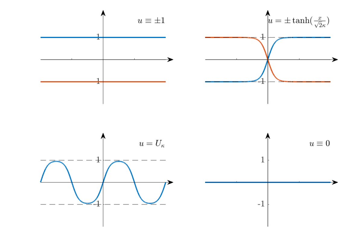
Figure 2. Classification of bounded steady states of Allen-Cahn ($\kappa=\frac{1}{2}$).

3. Classification of steady state energy

In this section, we consider the energy $E_{\kappa}(u)$ (see (1.5)) of solutions to (1.2). From the discussion of Section 2, we see that a nontrivial bounded steady state is a $2\pi$-periodic function. Therefore, we focus on the following problem

$$\kappa^{2}u^{\prime\prime}+u-u^{3}=0,\quad u(x)=u(x+2\pi)~{}\mbox{for}~{}x\in\mathbb{R}.$$ (3.1)

For simplicity of presentation, we introduce the following definition.

Definition 3.1 (Odd zero-up solution).

We shall say that $u$ is an odd zero-up solution to (3.1) if the solution $u$ is odd and $u^{\prime}(0)>0$.

Definition 3.2 (Odd zero-up ground states).

For each $0<\kappa<1$, we define $U_{\kappa}=u_{\kappa}$, where $u_{\kappa}$ is obtained in Proposition 2.3 as the odd zero-up ground state solution to (3.1). We also define the odd zero-up ground state energies $E_{\kappa}^{(0)}$ as

$$E_{\kappa}^{(0)} =\int_{\mathbb{T}}\Bigl{(}\frac{1}{2}\kappa^{2}(U_{\kappa}^{\prime}(x))^{2}+\frac{1}{4}(U_{\kappa}(x)^{2}-1)^{2}\Bigr{)}dx$$ (3.2)

$$=\int_{\mathbb{T}}\Bigl{(}\frac{1}{2}(U_{\kappa}(x)^{2}-1)^{2}-\frac{1}{4}(N_{\kappa}^{2}-1)^{2}\Bigr{)}dx,$$

where we recall $0<N_{\kappa}<1$ is the unique number satisfying

$$\int_{0}^{\frac{\pi}{2}}\frac{1}{\sqrt{2-N_{\kappa}^{2}(1+\sin^{2}\theta)}}d\theta=\frac{\pi}{2\sqrt{2}\kappa}.$$ (3.3)

For any solution of (3.1), we assume that its minimal period is $2\pi/m$ for some suitable positive integer $m$. From the proof of Proposition 2.4, it is not difficult to see that $u(x)$ has $2m$ zero points in $[x,x+2\pi)$ for any $x\in\mathbb{R}$ and $u(x)$ has odd symmetry with respect to any zero point. In addition, we can easily prove that the distance between any two consecutive zero points is same and equals to $2\pi/m$. After a suitable shift of the solution, we may assume $u(0)=0$ and $u$ is odd. On the other hand, if $u(x)$ is a solution to (3.1), obviously $u(-x)$ is also a solution. Hence, we may assume that $u^{\prime}(0)>0$ after reflection if necessary. Therefore, in this section we shall restrict our discussion on the odd zero-up solutions of equation (3.1). Concerning all the odd zero-up solutions to (3.1), we have the following classification result

Theorem 3.3 (Classification of odd zero-up solutions to (3.1)).

For any $0<\kappa<1$, define $m_{\kappa}\geq 1$ as the unique integer such that

$$\frac{1}{m_{\kappa}+1}\leq\kappa<\frac{1}{m_{\kappa}}.$$ (3.4)

Then there are only $m_{\kappa}$ odd zero-up solutions to (3.1). More precisely the following hold:

For each $j=1,\cdots,m_{\kappa}$, define (note below that $j\kappa<1$)

$$\tilde{u}_{\kappa,j}(x)=U_{j\kappa}(jx).$$ (3.5)

Then $\{\tilde{u}_{\kappa,j}\}_{j=1}^{m_{\kappa}}$ are all the possible odd zero-up solutions to (3.1). Furthermore the energies of $\tilde{u}_{\kappa,j}$ are given by

$$E_{\kappa,j} =\int_{\mathbb{T}}\Bigl{(}\frac{1}{2}(\kappa\partial_{x}{\tilde{u}_{\kappa,j}})^{2}+\frac{1}{4}(\tilde{u}_{\kappa,j}^{2}-1)^{2}\Bigr{)}dx=E_{j\kappa}^{(0)},$$ (3.6)

where $E_{j\kappa}^{(0)}$ was defined in (3.2).

Proof.

Suppose $u$ is a possible odd zero-up solution to (3.1). The crucial observation is that we must have $u$ achieves its first peak at $x=\frac{\pi}{2j}$ for some integer $j\geq 1$. Now make a change of variable $y=jx$, and $\tilde{u}(y)=u(x)$. Then clearly

$$j^{2}\kappa^{2}\frac{d^{2}}{dy^{2}}\tilde{u}-\tilde{u}+\tilde{u}^{3}=0,$$ (3.7)

$\tilde{u}(0)=0$, $\tilde{u}^{\prime}(0)>0$, and $\tilde{u}^{\prime}(\frac{\pi}{2})=0$. From the proof in Step 3 of Proposition 2.3, there exists a unique solution $u$ with $|u|<1$ solving the equation

$$u^{\prime}=\frac{1}{\sqrt{2}\kappa}\sqrt{(1-u^{2})^{2}-(1-N_{\kappa}^{2})^{2}},$$ (3.8)

with $u(0)=0$, $u^{\prime}(\frac{\pi}{2})=0$. As a consequence, we obtain that $\tilde{u}=U_{j\kappa}$. Now note that $j\kappa<1$ and this gives the constraint $j\leq m_{\kappa}$. The characterization (3.6) follows from the fact that

$$E_{\kappa,j} =\int_{\mathbb{T}}\Bigl{(}\frac{1}{2}(\tilde{u}_{\kappa,j}(x)^{2}-1)^{2}-\frac{1}{4}(N_{j\kappa}^{2}-1)^{2}\Bigr{)}dx$$

$$=\int_{\mathbb{T}}\Bigl{(}\frac{1}{2}(U_{j\kappa}(jx)^{2}-1)^{2}-\frac{1}{4}(N_{j\kappa}^{2}-1)^{2}\Bigr{)}dx,$$ (3.9)

and the fact that $U_{j\kappa}$ is $2\pi$-periodic. ∎

By Theorem 3.3 one can easily get Theorem 1.1. We notice that the $C^{0}$ estimate in the point (d) of Theorem 1.2 follows easily by (2.12). While for the point (e), one can easily prove it by some direct computations. For the left conclusions in Theorem 1.2, we rephrase it as the following result for the odd zero-up solutions

Theorem 3.4 (Monotonicity and asymptotics of odd zero-up ground state energies).

For any $\kappa>0$, define

$$\tilde{E}_{\kappa}=\inf_{u\in\mathcal{S}_{O}}\int_{\mathbb{T}}\Bigl{(}\frac{1}{2}(\kappa\partial_{x}u)^{2}+\frac{1}{4}(u^{2}-1)^{2}\Bigr{)}dx,$$ (3.10)

where

$$\mathcal{S}_{O}=\{\phi\mid\text{$\phi:\;\mathbb{T}\to\mathbb{R}$ is odd and $C^{1}$},~{}\phi^{\prime}(0)>0\}.$$ (3.11)

Then we have

• $\tilde{E}_{\kappa}=\frac{\pi}{2}$ for $\kappa\geq 1$. Furthermore

  $$\int_{\mathbb{T}}\Bigl{(}\frac{1}{2}(\kappa\partial_{x}u)^{2}+\frac{1}{4}(u^{2}-1)^{2}\Bigr{)}dx>\frac{\pi}{2}$$ (3.12)

  for any $u$ not identically zero.

• $\tilde{E}_{\kappa}=E_{\kappa}^{(0)}$ for $0<\kappa<1$. Moreover the infimum is only achieved by $U_{\kappa}$.

• If $0<\kappa_{1}<\kappa_{2}\leq 1$, then $\tilde{E}_{\kappa_{1}}<\tilde{E}_{\kappa_{2}}$.

Furthermore

$$\lim_{\kappa\to 0}\frac{E_{\kappa}^{(0)}}{{\kappa}}=\gamma_{*}=\frac{4}{3}\sqrt{2}>0.$$ (3.13)

Before proving Theorem 3.4, we establish the following important lemma.

Lemma 3.5.

Let $U_{\kappa}$ be the odd zero-up ground state to (3.1). Suppose that $0<\kappa_{1}<\kappa_{2}<1$, then we have

$$U_{\kappa_{1}}(x)>U_{\kappa_{2}}(x),\quad x\in\left(0,\frac{\pi}{2}\right].$$ (3.14)

Proof.

At first, we notice that $U_{\kappa}(0)=0$, $U^{\prime}_{\kappa}$ is monotone increasing for $x\in\left(0,\frac{\pi}{2}\right).$ By equation (2.35) we have

$$U^{\prime}_{\kappa}(x)=\frac{\sqrt{(1-U^{2}_{\kappa}(x))^{2}-(1-N^{2}_{\kappa})^{2}}}{\sqrt{2}\kappa},\quad\mbox{for}~{}x\in\left(0,\frac{\pi}{2}\right),$$ (3.15)

where $N_{\kappa}$ is the maximal value of $u_{\kappa}$ in $[0,\frac{\pi}{2}]$, i.e., $N_{\kappa}=U_{\kappa}(\frac{\pi}{2})$. By (3.15) we have

$$\int_{0}^{x}\frac{U^{\prime}_{\kappa}(x)}{\sqrt{U_{\kappa}^{4}(x)-2U_{\kappa}^{2}(x)+2N_{\kappa}^{2}-N_{\kappa}^{4}}}dx=\frac{x}{\sqrt{2}\kappa},\quad x\in\left(0,\frac{\pi}{2}\right),$$ (3.16)

which is equivalent to

$$\int_{0}^{U_{\kappa}(x)}\frac{\kappa}{\sqrt{s^{4}-2s^{2}+2N_{\kappa}^{2}-N_{\kappa}^{4}}}ds=\frac{x}{\sqrt{2}},\quad x\in\left(0,\frac{\pi}{2}\right).$$ (3.17)

If $0<\kappa_{1}<\kappa_{2}<1$, we have $1>N_{\kappa_{1}}>N_{\kappa_{2}}>0$ by equation (3.3). This implies that

$$1>2N_{\kappa_{1}}^{2}-N_{\kappa_{1}}^{4}>2N_{\kappa_{2}}^{2}-N_{\kappa_{2}}^{4}>0.$$ (3.18)

Therefore for any $s\in(0,\min\{N_{\kappa_{1}},N_{\kappa_{2}}\})$ we have

$$\frac{\kappa_{1}}{\sqrt{s^{4}-2s^{2}+2N_{\kappa_{1}}^{2}-N_{\kappa_{1}}^{4}}}<\frac{\kappa_{2}}{\sqrt{s^{4}-2s^{2}+2N_{\kappa_{2}}^{2}-N_{\kappa_{2}}^{4}}}.$$ (3.19)

Together with (3.17) we derive that $U_{\kappa_{1}}(x)>U_{\kappa_{2}}(x)$ for $x\in\left(0,\frac{\pi}{2}\right]$. This proves the lemma. ∎

Proof of Theorem 3.4..

We shall prove Theorem 3.4 point by point. For point (a), we notice that $u\equiv 0$ is the only odd zero-up solution to (3.1) whenever $\kappa\geq 1$. Then it is easy to verify that $\tilde{E}_{\kappa}=\frac{\pi}{2}$ for $\kappa\geq 1$.

Next, we consider the point (b). For any $2\pi$-periodic odd zero-up solution of (3.1) which is different by $U_{\kappa}$, we denote its minimal period by $2\pi/m$ and the solution by $u_{m},~{}m\geq 2$. Consider the function

$$v(y)=u_{m}(x),\quad y=mx.$$ (3.20)

Then it is not difficult to verify that

$$v(x)=U_{m\kappa}(x)\quad\mathrm{and}\quad x\in\left(0,\frac{\pi}{2}\right).$$ (3.21)

By Lemma 3.5, for $m\geq 2$ we have

$$U_{\kappa}(x)<U_{m\kappa}(x)\quad\mbox{for}\quad x\in\left(0,\frac{\pi}{2}\right).$$ (3.22)

On the other hand, we notice that

$$E^{(0)}_{\kappa}={} \int_{0}^{\frac{\pi}{2}}\left(2\kappa^{2}U_{\kappa}^{\prime 2}+(1-U_{\kappa}^{2})^{2}\right)dx$$ (3.23)

$$={} 2\kappa^{2}U_{\kappa}U_{\kappa}^{\prime}\mid_{x=0}^{x=\frac{\pi}{2}}+\int_{0}^{\frac{\pi}{2}}\left(-2\kappa^{2}U_{\kappa}U^{\prime\prime}_{\kappa}+(1-U_{\kappa}^{2})^{2}\right)dx$$

$$={} \int_{0}^{\frac{\pi}{2}}(1-U_{\kappa}^{4})dx.$$

Using (3.22) we have

$$E^{(0)}_{\kappa}>E^{(0)}_{m\kappa}.$$ (3.24)

By equation (3.6) we get

$$E^{(0)}_{m\kappa}=E(u_{m})=\int_{\mathbb{T}}\left(\frac{1}{2}(\kappa u_{m})^{2}+\frac{1}{4}(u_{m}^{2}-1)^{2}\right)dx.$$ (3.25)

Together with (3.24) we obtain that

$$E^{(0)}_{\kappa}=\tilde{E}_{\kappa},$$ (3.26)

and it proves the point (b).

The point (c) follows easily by point (b), Lemma 3.5 and equation (3.23).

In the end, we shall show the asymptotics as $\kappa\to 0$. By Proposition 2.3, the main part of $U_{\kappa}$ on $[-\frac{\pi}{2},\frac{\pi}{2}]$ is given by $\tanh(\frac{x}{\sqrt{2}\kappa})$. The result (3.13) then follows from a simple computation

$$\gamma_{*}={\sqrt{2}}\int_{\mathbb{R}}(\tanh^{2}y-1)^{2}dy={\sqrt{2}}\int_{\mathbb{R}}(1-\tanh^{2}y)\,d\tanh y=\frac{4}{3}{\sqrt{2}},$$ (3.27)

where $y=\frac{x}{\sqrt{2}\kappa}$. ∎

Corollary 3.6.

For any $0<\kappa<1$, if $u_{0}$ is odd, $2\pi$-periodic (monotonicity of $u_{0}$ is not required), and $E(u_{0})<E_{2\kappa}^{(0)}$, then the steady state of (1.1) is $\pm U_{\kappa}$, where $U_{\kappa}$ be the odd zero-up ground state to (3.1).

Proof.

Obviously, we have $E_{\kappa}^{(0)}\leq E(u_{0})<E_{2\kappa}^{(0)}$. From the energy dissipation property of (1.1), we can claim that $2\pi$ is the minimal period of the steady state for the initial condition $u_{0}$. ∎

4. Convergence to the steady state

In this section, we investigate the convergence rate of the solution and characterize the detailed profiles as $t\to\infty$.

4.1. Case of $0<\kappa<1$

We start this subsection with the following result on the spectrum analysis. This is crucial in showing the convergence rate is exponential

Lemma 4.1.

Let $0<\kappa<1$. Assume $U_{\kappa}$ is the odd zero-up ground state. Then for any $2\pi$-periodic odd function $\phi\in H^{1}(\mathbb{T})$ we have

$$\int_{\mathbb{T}}\kappa^{2}|\phi^{\prime}|^{2}dx+\int_{\mathbb{T}}\left(3U_{\kappa}^{2}-1\right)|\phi|^{2}dx\geq C\|\phi\|^{2}_{H^{1}(\mathbb{T})}$$ (4.1)

for some universal constant $C>0$.

Proof.

First of all, we notice that $C\geq 0$ due to the fact $U_{\kappa}$ is the odd zero-up ground state. Next, we shall prove that $C>0$ by contradiction. Suppose that $C=0$ then we can find a sequence of odd functions $\phi_{n}$ such that $\|\phi_{n}\|_{H^{1}(\mathbb{T})}=1$ and

$$\int_{\mathbb{T}}\kappa^{2}|\phi_{n}^{\prime}|^{2}dx+\int_{\mathbb{T}}\left(3U_{\kappa}^{2}-1\right)|\phi_{n}|^{2}dx\leq\frac{1}{n}.$$ (4.2)

Passing to a subsequence if necessary, we obtain there exists a nontrivial odd function $\phi_{*}\in H^{1}(\mathbb{T})$ such that $\phi_{n}$ weakly converges to $\phi_{*}$ in $H^{1}(\mathbb{T})$ and

$$\kappa^{2}\phi_{*}^{\prime\prime}+(1-3U_{\kappa}^{2})\phi_{*}=0\quad\mathrm{on}\quad\mathbb{T}.$$ (4.3)

After direct computations we see that

$$E_{\kappa}(U_{\kappa}+c\phi_{*})={} E_{\kappa}(U_{\kappa})+\frac{c^{2}}{2}\int_{\mathbb{T}}\left(\kappa^{2}|\phi_{*}^{\prime}|^{2}+(3U_{\kappa}^{2}-1)|\phi_{*}|^{2}\right)dx$$ (4.4)

$$+\int_{\mathbb{T}}\left(c^{3}U_{\kappa}\phi_{*}^{3}+\frac{c^{4}}{4}\phi_{*}^{4}\right)dx$$

for any real number $c$. Here we have used $U_{\kappa}$ is the odd zero-up ground state. Using (4.3) we see that the second term on the right hand side of (4.4) vanishes, then together with $E_{\kappa}(U_{\kappa}+c\phi_{*})\geq E_{k}(U_{\kappa})$ for any $c$, we see that

$$\int_{\mathbb{T}}U_{k}\phi_{*}^{3}=0.$$ (4.5)

It implies that $\phi_{*}$ must possess a zero point in $(0,\pi),$ denoted by $x_{*}$. By the well-known Strum Comparison Theorem (see [16, Theorem VI-1-1] for instance) we derive that any solution of the following equation must have a zero point in $(0,x_{*}),$

$$\phi^{\prime\prime}+(1-U_{\kappa}^{2})\phi=0.$$ (4.6)

However, we notice that $U_{k}$ is a solution of (4.6) and positive in $(0,\pi)$. Hence we arrive at a contradiction and the lemma is proved. ∎

With above lemma, we are now able to establish the proof of Theorem 1.4.

Proof of Theorem 1.4..

By smoothing estimates we may assume with no loss that $u_{0}\in C^{\infty}.$ It is not difficult to check that $u(x,t)$ is a $2\pi$-periodic odd function and also odd symmetric with respect to $x=\pi.$ Therefore

$$u(0,t)=u(\pi,t)\equiv 0,\quad\forall~{}t\geq 0.$$ (4.7)

Together with that $u_{0}(x)$ is non-negative in $[0,\pi]$, we conclude that $u(x,t)\geq 0$ for $x\in[0,\pi]$ by Maximum Principle, see [13, Section 2] for instance. Similarly, we have $u(x,t)\leq 0$ for $x\in[-\pi,0].$ Now by using the energy conservation we have

$$\frac{d}{dt}\left(\frac{1}{2}\|\partial_{x}u\|_{2}^{2}+\int_{\mathbb{T}}F(u)dx\right)=-\|\partial_{t}u\|_{2}^{2}.$$ (4.8)

where $F(u)=\frac{1}{4}(u^{2}-1)^{2}$. It follows that $\|\partial_{t}u\|_{L_{t}^{1}L_{x}^{2}}<\infty$ and one can extract a subsequence such that $\partial_{t}u(t_{n})\to 0$ in $L^{2}$. By using higher uniform Sobolev estimates one can obtain convergence in higher norms. In particular we can obtain $u(t_{n})\to u_{\infty}$ for some steady state of (3.1). In addition, $u_{\infty}$ is a $2\pi$-periodic odd function and non-negative for $x\in[0,\pi]$. By the proof of Theorem 1.1 we see that $0$ and $U_{\kappa}$ are the only steady states which are non-negative in $[0,\pi]$. As a consequence, we derive that $u_{\infty}$ could be either $U_{\kappa}$ or the trivial solution $0$.

If $E_{\kappa}(u_{0})\leq\frac{\pi}{2}$ and $u_{0}(x)\neq 0$, using (4.8) we see that

$$E_{\kappa}(u_{\infty})\leq E_{\kappa}(u_{0})\leq\frac{\pi}{2}.$$ (4.9)

The equality sign holds only $u_{\infty}=u_{0}$. While it is known that $E_{\kappa}(0)=\frac{\pi}{2}$ and $u_{0}\neq 0$. Then we get $u_{\infty}=U_{\kappa}$. To obtain exponential convergence, we can take $t_{n}$ sufficiently large such that $u(t_{n})$ is sufficiently close to the steady state $u_{\kappa}$. Combined with Lemma 4.1 we then obtain the exponential convergence. Thus, we finish the whole proof. ∎

Remark 4.2.

If the initial data $u_{0}$ is $2\pi$-periodic and satisfies

$$\left\{\begin{aligned} &u_{0}(x)=-u_{0}(-x),\quad\forall~{}x\in\mathbb{R},\\ &u_{0}^{\prime}(x)>0,~{}u_{0}(x)=u_{0}(\pi-x),\quad\quad~{}\forall~{}x\in\left(0,\frac{\pi}{2}\right).\end{aligned}\right.$$ (4.10)

Then by Theorem 1.4 we can prove that $u(x,t)\to U_{\kappa}$ as $t\to\infty$ whenever $E_{\kappa}(u_{0})\leq\frac{\pi}{2}.$ A typical example of the initial data satisfying (4.10) is $u_{0}(x)=\sin x$. More examples can be easily constructed along these lines.

Before we end the study for the case $\kappa\in(0,1)$, we present the following result establishing an useful property of the odd zero-up ground state. This part is of independent interest.

Lemma 4.3.

Fix $\kappa\in[\frac{1}{2},1)$ and assume $U_{\kappa}$ is the unique odd zero-up ground state for the equation

$$\kappa^{2}u^{\prime\prime}+u-u^{3}=0\quad\mbox{on}\quad\mathbb{T}=[-\pi,\pi].$$

Suppose that $u\in H^{1}(\mathbb{T})$ is an odd function on $\mathbb{T}$ with

$$E_{\kappa}(u)=\int_{\mathbb{T}}\left(\frac{1}{2}\kappa^{2}(u^{\prime})^{2}+\frac{1}{4}(u^{2}-1)^{2}\right)dx<\frac{\pi}{2}-C_{\kappa},$$ (4.11)

where $C_{\kappa}$ is a positive constant depending on $\kappa.$ Then we have

$$\min\{\|u-U_{\kappa}\|_{H^{1}(\mathbb{T})},~{}\|u+U_{\kappa}\|_{H^{1}(\mathbb{T})}\}\leq C\sqrt{E(u)-E(U_{\kappa})},$$ (4.12)

where $C>0$ is an absolute constant.

Remark 4.4.

In the special case $\kappa=0.9$, we can take $C_{\kappa}=0.001$. For the case $\kappa\in(0,\frac{1}{2})$, there are multiple steady-states and we shall address this issue elsewhere.

Proof.

We first claim that for odd $u\in H^{1}(\mathbb{T})$, when $E(u)-E(U_{\kappa})\rightarrow 0$, we must have

$$\min\{\|u-U_{\kappa}\|_{H^{1}(\mathbb{T})},~{}\|u+U_{\kappa}\|_{H^{1}(\mathbb{T})}\}\rightarrow 0.$$ (4.13)

We shall prove this by contradiction. Suppose the statement is not true, then for some $c_{0}>0$, there exists a sequence of odd functions $\{u_{n}\}$ such that

$$E(u_{n})-E(U_{\kappa})\leq\frac{1}{n},$$ (4.14)

and

$$\min\{\|u_{n}-U_{\kappa}\|_{H^{1}(\mathbb{T})},~{}\|u_{n}+U_{\kappa}\|_{H^{1}(\mathbb{T})}\}\geq c_{0}>0.$$ (4.15)

Using (4.14) we can find a universal constant $C$ such that

$$\int_{\mathbb{T}}|u^{\prime}_{n}|^{2}dx+\int_{\mathbb{T}}(1-u_{n}^{2})^{2}dx\leq C,$$ (4.16)

which implies that $\{u_{n}\}$ is a sequence of odd functions, and bounded in $H^{1}(\mathbb{T})$. Then we could select a subsequence, still denoted by $\{u_{n}\}$, such that

$$u_{n}~{}\mbox{ converge weakly to}~{}u_{*}~{}\mbox{in}~{}H^{1}(\mathbb{T}),$$ (4.17)

for some odd function $u_{*}\in H^{1}(\mathbb{T}).$ By the Rellich Lemma and lower semi-continuity of weak convergence, we have

$$E(U_{\kappa})\leq E(u_{*})\leq\liminf_{n\to+\infty}E(u_{n})=E(U_{\kappa}).$$ (4.18)

This implies that $E(U_{\kappa})=E(u_{*})$. Then we conclude that $u_{*}$ is either $U_{\kappa}$ or $-U_{\kappa}.$ Thus

$$u_{n}~{}\mbox{strongly converge to}~{}U_{\kappa}~{}\mbox{or}~{}-U_{\kappa}~{}\mbox{in}~{}H^{1}(\mathbb{T}).$$ (4.19)

This contradicts to (4.15). Therefore, the claim holds.

By using the claim, to establish (4.12), it suffices for us to consider the situation

$$\min\{\|u_{n}-U_{\kappa}\|_{H^{1}(\mathbb{T})},~{}\|u_{n}+U_{\kappa}\|_{H^{1}(\mathbb{T})}\}\ll 1.$$ (4.20)

In this case, without loss of generality we assume that $u^{\prime}(0)\geq 0$ and denote $\eta=u-U_{\kappa}$. Then it is not difficult to check that

$$E(u)-E(U_{\kappa})=\frac{1}{2}\int_{\mathbb{T}}\left[\kappa^{2}(\partial_{x}\eta)^{2}+(3U_{\kappa}^{2}-1)\eta^{2}\right]dx+O(\|\eta\|_{H^{1}}^{3})$$ (4.21)

By Lemma 4.1, we have

$$\frac{1}{2}\int_{\mathbb{T}}\left[\kappa^{2}(\partial_{x}\eta)^{2}+(3U_{\kappa}^{2}-1)\eta^{2}\right]dx\geq C\|\eta\|_{H^{1}}^{2},$$ (4.22)

where $C>0$ is an absolute constant. The desired conclusion follows easily. ∎

4.2. Case of $\kappa\geq 1$

In the case of $\kappa\geq 1$, we consider the a general Allen-Cahn equation

$$\begin{cases}\partial_{t}u=-\kappa^{2}\Lambda^{\gamma}u-(u^{3}-u),\qquad(x,t)\in\mathbb{T}\times(0,\infty),\\ u\Bigr{|}_{t=0}=u_{0},\end{cases}$$ (4.23)

where $\Lambda^{\gamma}=(-\partial_{xx})^{\gamma/2}$ is the fractional Laplacian of order $\gamma\in(0,2)$. When $\gamma=2$ it coincides with $-\partial_{xx}$.

Proposition 4.5 (Preliminary properties of steady states for $0<\gamma<1$).

Let $0<\gamma<2$ and $\kappa>0$. Suppose $\phi:\mathbb{T}\to\mathbb{R}$ is $C^{1,1}$ and satisfies

$$-\kappa^{2}\Lambda^{\gamma}\phi-(\phi^{2}-1)\phi=0.$$ (4.24)

Then $\phi\in C^{\infty}(\mathbb{T})$, and only one of the following occur:

• $\phi\equiv 1$;

• $\phi\equiv-1$ ;

• $\|\phi\|_{\infty}<1$.

Proof.

This follows from the usual maximum principle argument using the expression

$$(\Lambda^{\gamma}\phi)(x)=C_{\gamma}\sum_{n\in\mathbb{Z}}\operatorname{PV}\int_{|y|<\pi}\frac{\phi(x)-\phi(y)}{|x-y+2n\pi|^{1+\gamma}}dy.$$ (4.25)

Alternatively one can also derive the result using harmonic extension. ∎

To state the next result, we introduce the Fourier projection operators $\Pi_{1}$, $\Pi_{\geq 2}$ such that for $f=\sum_{m\geq 1}f_{m}\sin mx$ (assume the series converges sufficiently fast),

$$\Pi_{1}f=f_{1}\sin x;\qquad\Pi_{\geq 2}f=\sum_{m\geq 2}f_{m}\sin mx.$$ (4.26)

In other words $\Pi_{1}$ is the projection to the first sine-mode, and $\Pi_{\geq 2}$ simply removes the first Fourier mode in the sine series expansion.

Theorem 4.6.

Let $\kappa\geq 1$ and $0<\gamma\leq 2$. Assume $u_{0}$ is $2\pi$ periodic, odd and bounded. Suppose $u$ is the solution to (4.23) corresponding to the initial data $u_{0}$. If $\kappa>1$, we have exponential decay

$$\|u(t,\cdot)\|_{2}\leq\|u_{0}\|_{2}e^{-(\kappa^{2}-1)t},\qquad\forall~{}t\geq 0;$$ (4.27)

$$\|u(t,\cdot)\|_{H^{10}}\leq\beta_{1}e^{-(\kappa^{2}-1)t},\qquad\forall~{}t\geq\frac{1}{2};$$ (4.28)

$$\|\Pi_{\geq 2}u(t,\cdot)\|_{H^{10}}\leq\beta_{2}e^{-\eta_{1}t},\qquad\forall~{}t\geq\frac{1}{2},$$ (4.29)

where $\beta_{1}>0$, $\beta_{2}>0$ depend on ($u_{0}$, $\gamma$, $\kappa$), and $\Pi_{\geq 2}$ was defined in (4.26). The constant $\eta_{1}>\kappa^{2}-1$ is given by

$$\eta_{1}=\min\{\kappa^{2}2^{\gamma}-1,\;3(\kappa^{2}-1)\}.$$ (4.30)

For $\kappa=1$, we have algebraic decay:

$$\|u(t,\cdot)\|_{2}\leq\frac{\sqrt{\pi}\|u_{0}\|_{2}}{\sqrt{t\|u_{0}\|_{2}^{2}+\pi}},\qquad\forall~{}t\geq 0;$$ (4.31)

$$\|u(t,\cdot)\|_{H^{10}}\leq\beta_{3}t^{-\frac{1}{2}},\qquad\qquad\forall~{}t\geq\frac{1}{2};$$ (4.32)

$$\|\Pi_{\geq 2}u(t,\cdot)\|_{H^{10}}\leq\beta_{4}t^{-\frac{3}{2}},\qquad\forall~{}t\geq\frac{1}{2},$$ (4.33)

where $\beta_{3}>0$, $\beta_{4}>0$ depend on ($u_{0}$, $\gamma$).

Remark 4.7.

For $\kappa>1$, higher (i.e. $H^{m}$, $m>10$) Sobolev norms of $u$ also decay exponentially but we shall not dwell on this issue here. Note that we state the decay result for $t\geq\frac{1}{2}$ to allow the smoothing effect to kick in. The number $\frac{1}{2}$ is for convenience only and it can be replaced by any other $t_{0}>0$ with suitable adjustment of the corresponding pre-factors in the estimates.

Proof.

First we note that for bounded initial data, local and global wellposedness is not an issue and we focus solely on the decay estimates.

For the $L^{2}$ decay estimates, first we assume $u_{0}$ is smooth, and in particular has a finite sine-series expansion. It follows that $u(t)$ must have a spectral gap. By using the Poincaré inequality we have

$$\|\Lambda^{\frac{\gamma}{2}}u\|_{L^{2}(\mathbb{T})}\geq\|u\|_{L^{2}(\mathbb{T})}.$$ (4.34)

By using the above estimate and the fact that $\kappa\geq 1$, we obtain

$$\frac{1}{2}\frac{d}{dt}(\|u\|_{2}^{2}) =-\kappa^{2}\|\Lambda^{\frac{\gamma}{2}}u\|_{2}^{2}+\|u\|_{2}^{2}-\|u\|_{4}^{4}\leq-(\kappa^{2}-1)\|u\|_{2}^{2}-\|u\|_{4}^{4}$$ (4.35)

$$\leq-(\kappa^{2}-1)\|u\|_{2}^{2}-\frac{1}{2\pi}\|u\|_{2}^{4},$$

where in the last step we have used the Hölder’s inequality. Then, we derive that in the case of $\kappa>1$,

$$\|u\|_{2}\leq\|u_{0}\|_{2}\,e^{-(\kappa^{2}-1)t},$$ (4.36)

while in the case of $\kappa=1$,

$$\|u\|_{2}\leq\frac{\sqrt{\pi}\|u_{0}\|_{2}}{\sqrt{t\|u_{0}\|_{2}^{2}+\pi}}.$$ (4.37)

By a simple approximation argument, both estimates also hold under the assumption that $u_{0}\in L^{\infty}$.

We now show (4.28). First by smoothing estimates and interpolation, we have

$$\|\partial_{x}^{10}(u(t,\cdot))\|_{2}\leq\alpha_{1}e^{-\kappa_{1}t},\qquad\forall\,t\geq\frac{1}{2},$$ (4.38)

where $\alpha_{1}>0$ depends on ($u_{0}$, $\gamma$, $\kappa$), and $\kappa_{1}>0$ depends only on $\kappa$. It follows easily that

$$\|\partial_{x}^{10}(u^{3}(t,\cdot))\|_{2}\leq\alpha_{2}e^{-\kappa_{1}t}\|\partial_{x}^{10}u(t,\cdot)\|_{2},\qquad\forall\,t\geq\frac{1}{2},$$ (4.39)

where $\alpha_{2}>0$ depends on ($u_{0}$, $\gamma$, $\kappa$). We now compute for $t\geq\frac{1}{2}$,

$$\frac{1}{2}\frac{d}{dt}(\|\partial_{x}^{10}u(t,\cdot)\|_{2}^{2}) \leq-\kappa^{2}\|\Lambda^{\frac{\gamma}{2}}\partial_{x}^{10}u\|_{2}^{2}+\|\partial_{x}^{10}u\|_{2}^{2}+\|\partial_{x}^{10}(u^{3})\|_{2}\|\partial_{x}^{10}u\|_{2}$$

$$\leq(-(\kappa^{2}-1)+\alpha_{2}e^{-\kappa_{1}t})\|\partial_{x}^{10}u\|_{2}^{2}.$$ (4.40)

Integrating in time then yields (4.28).

The proof of (4.29) is similar. Note that for all $t\geq\frac{1}{2}$,

$$\|\partial_{x}^{10}\Pi_{\geq 2}(u^{3}(t,\cdot))\|_{2}\leq\|\partial_{x}^{10}(u^{3}(t,\cdot))\|_{2}\leq\alpha_{3}e^{-3(\kappa^{2}-1)t},$$ (4.41)

where $\alpha_{3}>0$ depends on ($u_{0}$, $\gamma$, $\kappa$). With this we compute:

$$\frac{1}{2}\frac{d}{dt}(\|\partial_{x}^{10}\Pi_{\geq 2}u(t,\cdot)\|_{2}^{2})$$ (4.42)

$$\leq-\kappa^{2}\|\Lambda^{\frac{\gamma}{2}}\partial_{x}^{10}\Pi_{\geq 2}u\|_{2}^{2}+\|\partial_{x}^{10}\Pi_{\geq 2}u\|_{2}^{2}+\|\partial_{x}^{10}(u^{3})\|_{2}\|\partial_{x}^{10}\Pi_{\geq 2}u\|_{2}$$

$$\leq(-(\kappa^{2}2^{\gamma}-1))\|\partial_{x}^{10}\Pi_{\geq 2}u\|_{2}^{2}+\alpha_{3}e^{-3(\kappa^{2}-1)t}\|\partial_{x}^{10}\Pi_{\geq 2}u\|_{2}.$$

Thus (4.29) follows from a simple ODE argument.

Finally (4.33) follows from working with the system

$$\partial_{t}\Pi_{\geq 2}u=-\kappa^{2}\Lambda^{\gamma}\Pi_{\geq 2}u+\Pi_{\geq 2}u-\Pi_{\geq 2}(u^{3}),$$ (4.43)

and bootstrapping estimates using (4.31). The estimate (4.32) is obvious. We omit the details. ∎

We turn now to some (by now) standard log-convexity results.

Proposition 4.8.

(Log convexity for an almost-linear model) Suppose $\mathbb{H}$ is a real Hilbert space with inner product $\langle\cdot,\cdot\rangle$ and norm $\|\cdot\|$. Let $A$ be a symmetric operator on $\mathbb{H}$ with domain $\mathcal{D}(A)$. Let $T>0$ and $u\in C_{t}^{1}([0,T],\,\mathbb{H})$ satisfy $u(t)\in\mathcal{D}(A)$ for each $0<t<T$, and

$$\|\partial_{t}u+Au\|\leq\alpha(t)\|u(t)\|,\qquad\forall\,0<t<T,$$ (4.44)

where $\alpha(t)\geq 0$ satisfies

$$\int_{0}^{T}\alpha(t)^{2}dt<\infty.$$ (4.45)

Denote $m(t)=\|u(t)\|^{2}$. Then $m$ is log-convex:

$$m(t)\leq e^{\int_{0}^{T}(4\alpha(s)+s\alpha(s)^{2})ds}m(0)^{1-\frac{t}{T}}m(T)^{\frac{t}{T}},\qquad\forall\,0\leq t\leq T.$$ (4.46)

It follows that either $m(t)\equiv 0$ on $[0,T]$ or $m(t)>0$ for all $t\in[0,T]$.

Proof.

First we assume that $m(t)>0$ for all $0\leq t\leq T$. Denote $f=\partial_{t}u+Au$ so that

$$\partial_{t}u=-Au+f.$$ (4.47)

Denote

$$b_{1}=\frac{2}{m}\langle u,f\rangle.$$ (4.48)

Then clearly

$$\frac{d}{dt}\left(\ln m+\int_{t}^{T}b_{1}(s)ds\right)=\frac{2}{m}\langle u,-Au\rangle;$$ (4.49)

and

$$\frac{1}{4}\frac{d^{2}}{dt^{2}}\left(\ln m+\int_{t}^{T}b_{1}(s)ds\right)$$ (4.50)

$$=\frac{\langle u_{t},-Au\rangle}{m}-\frac{\langle u,-Au\rangle\langle u,-Au+f\rangle}{m^{2}}$$

$$=\frac{m\|Au\|^{2}-|\langle u,-Au\rangle|^{2}}{m^{2}}+\frac{\langle f,-Au\rangle}{m}+\frac{\langle u,Au\rangle\langle u,f\rangle}{m^{2}}.$$

We decompose $Au=c_{1}u+cu^{\perp}$ where $c_{1},c\in\mathbb{R}$ and $u^{\perp}$ is a unit vector orthogonal to $u$. Plugging this into the last expression, we obtain

$$\frac{1}{4}\frac{d^{2}}{dt^{2}}\left(\ln m+\int_{t}^{T}b_{1}(s)ds\right) =\frac{c^{2}}{m}-\frac{c\langle f,u^{\perp}\rangle}{m}$$ (4.51)

$$\geq\frac{(|c|-\frac{1}{2}|\langle f,u^{\perp}\rangle|)^{2}}{m}-\frac{1}{4}\frac{|\langle f,u^{\perp}\rangle|^{2}}{m}$$

$$\geq-\frac{1}{4}\alpha(t)^{2}.$$

It follows that $r(t)$ is convex, where

$$r(t)=\ln m(t)+\underbrace{\int_{t}^{T}b_{1}(s)ds+\int_{t}^{T}\int_{\tau}^{T}\alpha^{2}(s)dsd\tau}_{=:b(t)}.$$ (4.52)

From the convexity of $r(t)$ we deduce

$$r(t)\leq(1-\frac{t}{T})r(0)+\frac{t}{T}r(T).$$ (4.53)

This implies that

$$\ln m(t)\leq(1-\frac{t}{T})\ln m(0)+\frac{t}{T}\ln m(T)+(1-\frac{t}{T})b(0)+\frac{t}{T}b(T)-b(t).$$ (4.54)

Since $b(T)=0$ and $\int_{t}^{T}\int_{s}^{T}\alpha(\tau)^{2}d\tau ds\geq 0$, we obtain

$$(1-\frac{t}{T})b(0)+\frac{t}{T}b(T)-b(t) =(1-\frac{t}{T})b(0)-b(t)$$ (4.55)

$$\leq 2\int_{0}^{T}|b_{1}(s)|ds+\int_{0}^{T}\int_{\tau}^{T}\alpha^{2}(s)dsd\tau$$

$$\leq\int_{0}^{T}(4\alpha(s)+s\alpha(s)^{2})ds.$$

Thus the desired inequality holds under the assumption that $m(t)>0$ for all $t\in[0,T]$.

Now we show how to remove this assumption. Assume that $m(t)$ is not identically zero. Since $m(t)\geq 0$ is a continuous function of $t$ and $m(t)$ is not identically zero, we may assume that there exists $t_{0}\in[0,T]$ such that $m(t_{0})>0$. By a continuity argument we can assume $t_{0}\in(0,T)$. Now denote

$$t_{+}=\sup\{t:\;t>t_{0}\text{ such that $m(s)>0$ for all $t_{0}\leq s\leq t$}\};$$ (4.56)

$$t_{-}=\inf\{t:\;t<t_{0}\text{ such that $m(s)>0$ for all $t\leq s\leq t_{0}$}\}.$$ (4.57)

If $t_{+}<T$, then we have $m(t_{+})=0$ with $m(t)>0$ for all $t_{0}\leq t<t_{+}$. By using a version of the proved inequality on the interval $[t_{0},t_{+}-\eta]$ (note that $m(t)>0$ for all $t_{0}\leq t\leq t_{+}-\eta$ and thus we can use the proved inequality with the interval $[0,T]$ now replaced by $[t_{0},t_{+}-\eta]$) and sending $\eta\to 0$, we clearly obtain a contradiction. If $t_{+}=T$ and $m(T)=0$, we also obtain a contradiction by a similar argument. By a similar reasoning we obtain $t_{-}=0$ and $m(0)>0$. Thus we have proved that $m(t)>0$ for all $t\in[0,T]$. ∎

Lemma 4.9.

For any $0<\gamma\leq 2$, there exits $\eta_{0}=\eta_{0}(\gamma)>0$ such that the following hold for any smooth $2\pi$-periodic odd function $u$ on $\mathbb{T}$:

$$\int_{\mathbb{T}}u^{3}(-\partial_{xx})^{\frac{\gamma}{2}}udx\geq\eta_{0}\|u\|_{4}^{4}.$$ (4.58)

For $\gamma=2$, we can take $\eta_{0}=3/4$.

Proof.

This follows from a general result proved in [17]. For $\gamma=2$ we give a direct proof as follows (below we write $\int_{\mathbb{T}}dx$ as $\int$)

$$\int u^{3}(-\partial_{xx}u)=3\int(\partial_{x}u)^{2}u^{2}=\frac{3}{4}\int\Bigl{(}\partial_{x}(|u|u)\Bigr{)}^{2}dx\geq\frac{3}{4}\||u|u\|_{2}^{2}=\frac{3}{4}\|u\|_{4}^{4}.$$ (4.59)

Note that in the above we took advantage of the odd symmetry since the function $v=|u|u$ is still odd on $[-\pi,\pi]$. Note that regularity is not an issue here since the function $g(z)=|z|z$ is nice. ∎

Theorem 4.10 (Log convexity of $L^{2}$ mass for the nonlinear case).

Let $\kappa>0$ and $0<\gamma\leq 2$. Assume $u_{0}$ is $2\pi$ periodic, odd and bounded. To avoid triviality assume $\|u_{0}\|_{2}>0$ so that $u_{0}$ is not identically zero. Suppose $u$ is the solution to (4.23) corresponding to the initial data $u_{0}$. Denote $m(t)=\|u(t)\|_{L_{x}^{2}(\mathbb{T})}^{2}$. Then the following hold.

• If $0<\kappa<1$, then $m(t)$ is log-convex on any interval $0\leq t_{1}<t_{2}$:

  $$m(t)\leq e^{c_{1}\cdot(t_{2}-t_{1})^{2}}m(t_{1})^{1-\frac{t-t_{1}}{t_{2}-t_{1}}}m(t_{2})^{\frac{t-t_{1}}{t_{2}-t_{1}}},\qquad\forall\,t\in(t_{1},t_{2}),$$ (4.60)

  where $c_{1}>0$ is a constant depending only on ($\|u_{0}\|_{\infty}$, $\gamma$, $\kappa$).

• If $\kappa>1$, then $m(t)$ is log-convex on any interval $0\leq t_{1}<t_{2}$:

  $$m(t)\leq c_{2}m(t_{1})^{1-\frac{t-t_{1}}{t_{2}-t_{1}}}m(t_{2})^{\frac{t-t_{1}}{t_{2}-t_{1}}},\qquad\forall\,t\in(t_{1},t_{2}),$$ (4.61)

  where $c_{2}>0$ is a constant depending only on ($\|u_{0}\|_{\infty}$, $\gamma$, $\kappa$).

• If $\kappa=1$, then $m(t)$ is log-convex on any interval $0\leq t_{1}<t_{2}$:

  $$m(t)\leq(1+t_{2}-t_{1})^{c_{3}}m(t_{1})^{1-\frac{t-t_{1}}{t_{2}-t_{1}}}m(t_{2})^{\frac{t-t_{1}}{t_{2}-t_{1}}},\qquad\forall\,t\in(t_{1},t_{2}),$$ (4.62)

  where $c_{3}>0$ is a constant depending only on ($\|u_{0}\|_{\infty}$, $\gamma$, $\kappa$).

• For each $0<\gamma\leq 2$, there is $\kappa_{0}=\kappa_{0}(\gamma)>0$ such that if $\kappa\geq\kappa_{0}$, then we have sharp log-convexity, i.e.: on any interval $0\leq t_{1}<t_{2}$:

  $$m(t)\leq m(t_{1})^{1-\frac{t-t_{1}}{t_{2}-t_{1}}}m(t_{2})^{\frac{t-t_{1}}{t_{2}-t_{1}}},\qquad\forall\,t\in(t_{1},t_{2}),$$ (4.63)

  Furthermore for $\gamma=2$, we can choose $\kappa_{0}(2)=2/\sqrt{3}$.

Proof.

First we consider the case $0<\kappa<1$. Observe that

$$\|\partial_{t}u+\kappa^{2}\Lambda^{\gamma}u-u\|_{2}\leq\|u(t)\|_{L_{x}^{\infty}}^{2}\|u(t)\|_{2}.$$ (4.64)

It is not difficult to check that

$$\sup_{0\leq t<\infty}\|u(t)\|_{L_{x}^{\infty}}\leq\tilde{c}_{1},$$ (4.65)

where $\tilde{c}_{1}>0$ depends only on ($\|u_{0}\|_{\infty}$, $\gamma$, $\kappa$). Thus the result follows from Proposition 4.8.

Now for $\kappa>1$, we observe that by using Theorem 4.6 (note that for $0<s\leq\frac{1}{2}$ we have uniform control of $L^{\infty}$-norm), it holds that

$$\|u(s)\|_{L_{x}^{\infty}}\leq\tilde{c}_{2}e^{-\theta_{1}s},\qquad\forall\,s\geq 0,$$ (4.66)

where $\tilde{c}_{2}>0$ depends only on ($\|u_{0}\|_{\infty}$, $\gamma$, $\kappa$) and $\theta_{1}$ depends only on ($\kappa$, $\gamma$). Thus

$$\tilde{\alpha}(s):=\|u(s)\|_{L_{x}^{\infty}}^{2}\leq\tilde{c}_{2}^{2}e^{-2\theta_{1}s},\qquad\forall\,s\geq 0.$$ (4.67)

On any time interval $[t_{1},t_{2}]$ with $0\leq t_{1}<t_{2}$, in order to apply Proposition 4.8, we note for $t\geq 0$,

$$\alpha(t)=\tilde{\alpha}(t_{1}+t)\leq\tilde{c}_{2}^{2}e^{-2\theta_{1}t}.$$ (4.68)

Thus the desired result follows for $\kappa>1$.

The case for $\kappa=1$ follows similarly from Theorem 4.6 and Proposition 4.8. The main observation is that $\|u(s)\|_{L_{x}^{\infty}}=O((1+s)^{-\frac{1}{2}})$ for $s\geq 0$.

Finally we turn to the proof of (4.63). We shall appeal to a more “nonlinear” proof as follows. Denote $m(t)=\|u(t)\|_{L_{x}^{2}}^{2}$ and $A=\kappa^{2}(-\partial_{xx})^{\frac{\gamma}{2}}-1$. Thus we have

$$\partial_{t}u=-Au-u^{3}.$$ (4.69)

Denote $m^{\prime}=\frac{d}{dt}m$ and $m^{\prime\prime}=\frac{d^{2}}{dt^{2}}m$. It is not difficult to check that (below $\langle\cdot,\cdot\rangle$ denotes the usual $L^{2}$ inner product, and $u_{t}=\partial_{t}u$)

$$m^{\prime}=2\langle u,u_{t}\rangle=-2\langle u,Au\rangle-2\|u\|_{4}^{4};$$ (4.70)

$$m^{\prime\prime}=-4\langle u_{t},Au\rangle-8\langle u^{3},u_{t}\rangle.$$ (4.71)

Thus

$$\frac{1}{2}m^{\prime}=\langle u,u_{t}\rangle;$$ (4.72)

$$\frac{1}{4}m^{\prime\prime}=\|u_{t}\|_{2}^{2}-\langle u^{3},u_{t}\rangle;$$ (4.73)

$$\frac{1}{4}m^{\prime\prime}m-\frac{1}{4}(m^{\prime})^{2}=\|u_{t}\|_{2}^{2}\|u\|_{2}^{2}-|\langle u,u_{t}\rangle|^{2}+(\langle u^{3},Au\rangle+\|u\|_{6}^{6})\|u\|_{2}^{2}.$$ (4.74)

It remains for us to verify

$$\langle u^{3},Au\rangle=\kappa^{2}\int_{\mathbb{T}}u^{3}(-\partial_{xx})^{\frac{\gamma}{2}}udx-\|u\|_{4}^{4}\geq 0.$$ (4.75)

This in turn follows from Lemma 4.9. ∎

Corollary 4.11 (No finite time extinction of $L^{2}$ mass).

Let $\kappa>0$ and $0<\gamma\leq 2$. Assume $u_{0}$ is $2\pi$ periodic, odd and bounded. To avoid triviality assume $\|u_{0}\|_{2}>0$ so that $u_{0}$ is not identically zero. Suppose $u$ is the solution to (4.23) corresponding to the initial data $u_{0}$. Then $\|u(t)\|_{L_{x}^{2}}>0$ for any $0\leq t<\infty$.

Proof.

This follows easily from Proposition 4.10. ∎

Theorem 4.12 (Profiles as $t\to\infty$).

Let $\kappa\geq 1$ and $0<\gamma\leq 2$. Assume $u_{0}$ is $2\pi$ periodic, odd and bounded. To avoid triviality assume $\|u_{0}\|_{2}>0$ so that $u_{0}$ is not identically zero. Suppose $u$ is the solution to (4.23) corresponding to the initial data $u_{0}$. Then the following hold.

• Case $\kappa>1$. For all $t\geq 1$, we have

  $$u(x,t)=e^{-(\kappa^{2}-1)t}\alpha_{*}\sin x+r(t),$$ (4.76)

  where the constant $\alpha_{*}$ depends on ($u_{0}$, $\gamma$, $\kappa$). The remainder term $r(t)$ has the estimate

  $$\|r(t)\|_{H^{10}}\leq\tilde{\alpha}e^{-\eta_{1}t},\qquad\forall\,t\geq 1,$$ (4.77)

  with $\tilde{\alpha}>0$ depends only on ($u_{0}$, $\gamma$, $\kappa$), and $\eta_{1}=\min\{\kappa^{2}2^{\gamma}-1,\;3(\kappa^{2}-1)\}>\kappa^{2}-1$.

• Case $\kappa=1$. For all $t\geq 1$, we have

  $$u(x,t)=t^{-\frac{1}{2}}\beta_{*}\sin x+r_{1}(t),$$ (4.78)

  where the constant $\beta_{*}$ depends on ($u_{0}$, $\gamma$). If $\beta_{*}=0$, then the remainder term $r_{1}(t)$ has the estimate

  $$\|r_{1}(t)\|_{H^{10}}\leq\tilde{\beta}t^{-1}\sqrt{\ln(t+2)},\qquad\forall\,t\geq 1,$$ (4.79)

  with $\tilde{\beta}>0$ depends only on ($u_{0}$, $\gamma$). If $\beta_{*}\neq 0$, then the remainder term $r_{1}(t)$ has the estimate

  $$\|r_{1}(t)\|_{H^{10}}\leq\tilde{\beta}t^{-\frac{3}{2}}{\ln(t+2)},\qquad\forall\,t\geq 1,$$ (4.80)

  with $\tilde{\beta}>0$ depends only on ($u_{0}$, $\gamma$).

Remark 4.13.

Clearly, Theorem 1.3 follows from above result immediately. Note that for $\kappa>1$ and generic nontrivial odd periodic $u_{0}$ we could have $\alpha_{*}=0$. An easy example is $u_{0}(x)=\sin 2x$. On the other hand, a further interesting question is to investigate whether the following scenario is possible: namely if we denote

$$\alpha_{1}(t)=\int_{\mathbb{T}}u(t,x)\sin xdx.$$ (4.81)

then for some $t=t_{c}$, $\alpha_{1}(t)=0$ for $t\geq t_{c}$, and $\alpha_{1}(t)\neq 0$ for $t<t_{c}$ with $t_{c}-t$ sufficiently small.

Proof.

We first consider $\kappa>1$. Write

$$u=\Pi_{1}u+\Pi_{\geq 2}u,$$ (4.82)

where the operators $\Pi_{1}$, $\Pi_{\geq 2}$ were defined in (4.26). By Theorem 4.6 the term $\Pi_{\geq 2}u$ has the desired decay for $t\geq 1$ and can be included in the remainder $r(t)$. Thus we only need to treat the single-mode part $\Pi_{1}u$. Denote

$$\Pi_{1}u(t)=a(t)\sin x,\qquad a(t)=\frac{1}{\pi}\int_{\mathbb{T}}\Pi_{1}u(t,x)\sin xdx;$$ (4.83)

$$\Pi_{1}(-u^{3}(t))=b(t)\sin x,\qquad b(t)=\frac{1}{\pi}\int_{\mathbb{T}}\Pi_{1}(-u^{3}(t,x))\sin xdx.$$ (4.84)

By Theorem 4.6, we have for some $\tilde{C}>0$ depending only on ($u_{0}$, $\gamma$, $\kappa$),

$$|b(t)|\leq\tilde{C}e^{-3(\kappa^{2}-1)t},\qquad\forall\,t\geq\frac{1}{2}.$$ (4.85)

Clearly we have

$$\frac{d}{dt}a(t)=-(\kappa^{2}-1)a(t)+b(t).$$ (4.86)

We then write for $t\geq 1$,

$$a(t) =e^{-(\kappa^{2}-1)(t-\frac{1}{2})}a(\frac{1}{2})+\int_{\frac{1}{2}}^{t}e^{-(\kappa^{2}-1)(t-s)}b(s)ds$$

$$=e^{-(\kappa^{2}-1)t}\Bigl{(}e^{\frac{1}{2}(\kappa^{2}-1)}a(\frac{1}{2})+\int_{\frac{1}{2}}^{\infty}e^{(\kappa^{2}-1)s}b(s)ds\Bigr{)}+\tilde{r}(t),$$ (4.87)

where

$$|\tilde{r}(t)|\leq e^{-(\kappa^{2}-1)t}\int_{t}^{\infty}e^{(\kappa^{2}-1)s}|b(s)|ds=O(e^{-3(\kappa^{2}-1)t}).$$ (4.88)

Clearly then (4.76) follows.

The proof of (4.78) is slightly more intricate. We only need to treat the piece $\Pi_{1}u$ since the part $\Pi_{\geq 2}u$ can be included in the remainder term $r_{1}(t)$. Observe that for $t\geq\frac{1}{2}$, by Theorem 4.6 we have

$$u(t)^{3}=(\Pi_{1}u(t)+\Pi_{\geq 2}u(t))^{3}=(\Pi_{1}u)^{3}+\tilde{r}(t),$$ (4.89)

where

$$\|\tilde{r}(t)\|_{H^{10}}=O(t^{-\frac{5}{2}}),\qquad\forall\,t\geq\frac{1}{2}.$$ (4.90)

Denote $\Pi_{1}u(t)=a(t)\sin x$, clearly

$$\Pi_{1}((\Pi_{1}u(t))^{3})=\frac{3}{4}a(t)^{3}\sin x.$$ (4.91)

For $a(t)$ we have the ODE

$$\frac{d}{dt}a(t)=-\frac{3}{4}a(t)^{3}+b(t),\qquad t\geq\frac{1}{2},$$

where $|b(t)|=O(t^{-\frac{5}{2}})$.

Denote $\theta(t)=a(t)^{2}$. We clearly have

$$\frac{d}{dt}\theta(t)=-\frac{3}{2}\theta(t)^{2}+O(t^{-3}).$$ (4.92)

By Proposition 4.16 proved below, we have for $t\geq 3$,

$$\theta(t)=\frac{\theta_{*}}{t}+O(t^{-2}\ln t),$$ (4.93)

Note that $\theta_{*}\geq 0$ since $\theta(t)$ is always nonnegative.

Now if $\theta_{*}=0$ we can take $\beta_{*}=0$ and the desired result follows easily. If $\theta_{*}>0$, then $|a(t)|\sim t^{-1/2}$ for $t$ large. By continuity it can only take one sign. Thus we obtain $\beta_{*}=\sqrt{\theta_{*}}$ or $\beta_{*}=-\sqrt{\theta_{*}}$. The estimate for the remainder term is trivial. We omit the details. ∎

Lemma 4.14.

Assume $T_{0}\geq 1$. Suppose $\theta:\,[T_{0},\infty)\to[0,\infty)$ is continuously differentiable and safisfy

$$0<\limsup_{t\to\infty}t\theta(t)<\infty;\qquad\theta^{\prime}(t)\geq-\frac{3}{2}\theta^{2}(t)-t^{-2.2},\quad\forall\,t>T_{0}.$$ (4.94)

Then we have

$$\liminf_{t\to\infty}t\theta(t)>0.$$ (4.95)

Proof.

It is natural to appeal to a maximum principle argument. Denote

$$2\theta_{0}=\limsup_{t\to\infty}\theta(t)t>0.$$ (4.96)

Let

$$\Omega(t)=\theta(t)-\eta_{0}t^{-1},$$ (4.97)

where $\eta_{0}>0$ satisfies

$$\eta_{0}\leq\min\{\frac{1}{2}\theta_{0},\;\frac{1}{10}\}.$$ (4.98)

By (4.96), we can choose $t_{0}>0$ sufficiently large such that

$$\theta(t_{0})\geq\frac{\theta_{0}}{t_{0}},\qquad\frac{\eta_{0}}{2t_{0}^{2}}-t_{0}^{-2.2}>0.$$ (4.99)

Note that the second condition above guarantees that

$$\frac{\eta_{0}}{2t^{2}}-t^{-2.2}>0,\qquad\forall\,t\geq t_{0}.$$ (4.100)

Now consider $\Omega(t)$ on the time interval $[t_{0},\infty)$. If $\Omega(t)>0$ for all $t\geq t_{0}$ we are done. Otherwise there exists some time $t_{1}>t_{0}$ such that $\Omega(t_{1})=0$. But then clearly

$$\theta(t_{1})=\frac{\eta_{0}}{t_{1}};\qquad\Omega^{\prime}(t_{1})=-\frac{3}{2}\frac{\eta_{0}^{2}}{t_{1}^{2}}+\frac{\eta_{0}}{t_{1}^{2}}-t_{1}^{-2.2}\geq\frac{\eta_{0}}{2t_{1}^{2}}-t_{1}^{-2.2}>0.$$ (4.101)

Thus $\Omega(t)$ continuous to be positive a little bit past $t_{1}$. This argument then guarantees that $\Omega(t)\geq 0$ for all $t\geq t_{0}$. ∎

Lemma 4.15.

Assume $T_{0}\geq 1$ and $0<\kappa_{0}<1$. Suppose $\theta:\,[T_{0},\infty)\to[0,\infty)$ satisfies

$$\theta(t)\leq\frac{\kappa_{0}}{t}\quad\mathrm{and}\quad\theta(t)\leq\frac{1}{2}\int_{t}^{\infty}\theta(s)^{2}ds+\frac{1}{2t^{2}},\qquad\forall\,t\geq T_{0}.$$ (4.102)

Then there exists a constant $C_{1}>0$ depending on $\kappa_{0}$ and $T_{0}$, such that

$$\theta(t)\leq\frac{C_{1}}{t^{2}},\qquad\forall\,t\geq T_{0}.$$ (4.103)

Proof.

We begin by noting that, if we assume

$$\theta(t)\leq\frac{\alpha}{t},\qquad\forall\,t\geq\max\{T_{0},\;\frac{1}{\alpha}\}.$$ (4.104)

then we obtain

$$\theta(t)\leq\frac{1}{2}\cdot\frac{\alpha^{2}}{t}+\frac{1}{2t^{2}}\leq\frac{\alpha^{2}}{t},\qquad\forall\,t\geq\max\{T_{0},\;\frac{1}{\alpha^{2}}\}.$$ (4.105)

Now define $\alpha_{0}=\kappa_{0}<1$, and $\alpha_{k+1}=\alpha_{k}^{2}$. Note that

$$\alpha_{k}=e^{2^{k}\ln\kappa_{0}}.$$ (4.106)

Clearly it holds that

$$\theta(t)\leq\frac{\alpha_{k}}{t},\qquad\forall\,t\geq\max\{T_{0},\;\frac{1}{\alpha_{k}}\}.$$ (4.107)

Consider $t\in[\frac{1}{\alpha_{k}},\;\frac{1}{\alpha_{k+1}}]=[\frac{1}{\alpha_{k}},\frac{1}{\alpha_{k}^{2}}]$. Clearly it holds that

$$\alpha_{k}\leq t^{-\frac{1}{2}}.$$ (4.108)

Thus we have for all $t\in[\frac{1}{\alpha_{k}},\;\frac{1}{\alpha_{k+1}}]$ with $\frac{1}{\alpha_{k}}\geq T_{0}$, it holds that

$$\theta(t)\leq t^{-\frac{3}{2}}.$$ (4.109)

Thus we have for all $t$ sufficiently large

$$\theta(t)\leq t^{-\frac{3}{2}}.$$ (4.110)

Iterating this estimate again we obtain $\theta(t)\leq O(t^{-2})$. ∎

Proposition 4.16.

Assume $T\geq 3$. Suppose $\theta:\;[T,\infty)\to[0,\infty)$ is continuously differentiable and satisfy

$$\sup_{t\geq T_{0}}t\theta(t)<\infty;\qquad\theta^{\prime}(t)=-\frac{3}{2}\theta^{2}(t)+F(t),\quad\forall\,t>T,$$ (4.111)

where for some $K_{0}>0$

$$|F(t)|\leq K_{0}t^{-3},\qquad\forall\,t\geq T.$$ (4.112)

Then there exists $\theta_{*}\in\mathbb{R}$, such that

$$\theta(t)=\frac{\theta_{*}}{t}+R(t),$$ (4.113)

where

$$\sup_{t\geq T}\frac{|R(t)|}{\frac{\ln t}{t^{2}}}<\infty.$$ (4.114)

Proof.

Note that we only need to investigate the regime $t\gg 1$. We shall discuss two cases:

Case 1. $\limsup\limits_{t\to\infty}t\theta(t)>0$. In this case we use Lemma 4.14. Clearly for $T_{0}$ sufficiently large we have

$$\theta(t)t\sim 1,\qquad\forall\,t\geq T_{0}.$$ (4.115)

From the ODE we obtain

$$\frac{d}{dt}\Bigl{(}\frac{1}{\theta}\Bigr{)}=\frac{3}{2}+O(t^{-1}).$$ (4.116)

It follows that for $T_{0}^{\prime}$ sufficiently large and all $t\geq T_{0}^{\prime}+2$,

$$\theta(t)=\frac{1}{d_{1}+d_{2}(t-T_{0}^{\prime})+O(\ln(t-T_{0}^{\prime}))},$$ (4.117)

where $d_{1}>0$, $d_{2}>0$ are constants. The desired asymptotics then follows easily.

Case 2. $\limsup_{t\to\infty}\theta(t)t=0$. In this case we make a change of variable:

$$t=N\tau,\;\theta(t)=\gamma\Theta(\tau),\quad\frac{N}{\gamma}F(t)=\tilde{F}(\tau).$$ (4.118)

Clearly

$$\frac{d}{d\tau}\Theta(\tau)=-\frac{3}{2}\gamma N\Theta^{2}+\tilde{F}(\tau),\quad\mbox{and}\quad|\tilde{F}(\tau)|\leq K_{0}\frac{1}{\gamma N^{2}}\tau^{-3}.$$ (4.119)

Thus if we take $\gamma=\frac{1}{3N}$ and $N$ sufficiently large, we obtain

$$\Theta(\tau)\leq\frac{1}{2}\int_{\tau}^{\infty}\Theta^{2}(s)ds+\frac{1}{2\tau^{2}},\qquad\forall\,\tau\geq\tau_{0},$$ (4.120)

where $\tau_{0}$ is sufficiently large. We then use Lemma 4.15 to conclude that $\Theta(\tau)=O(\tau^{-2})$. Thus in this case $\theta(t)=O(t^{-2})$. ∎

5. Concluding remarks.

In this work we considered the classification of steady states to the one-dimensional periodic Allen-Cahn equation with standard double well potential. We gave a full classification of all possible steady states and identitified their precise dependence on the diffusion coefficient in terms of energy and profiles. We found a novel self-replicating property of steady state solutions amongst the hierarchy solutions organized according to the diffusion parameter. We developed a new modulation theory around these steady states and proved sharp convergence results. We discuss below a few possible future directions.

• Classification for other models with different linear dissipations and nonlinearities. Even for the classical Allen-Cahn case, one can investigate the singular potential functions such as the logarithmic function given by

  $$f(u)=-u+\frac{1}{8}\log\frac{1+u}{1-u},$$ (5.1)

  or the sine-Gordon type

  $$f(u)=-\sin u.$$ (5.2)

  Besides the one dimensional theory, we also expect some generalizations to higher dimensions.

• Patching and extension and solutions across general interfaces. It is natural to consider extending solutions of

  $$\mathcal{L}u-f(u)=0\quad\mbox{in}\quad\Omega,$$ (5.3)

  where $\mathcal{L}$ is the linear part and $f$ denotes the nonlinear part with appropriate boundary conditions. The task is to investigate under what conditions we can extend the solution across a portion of the boundary of $\Omega$ which is assumed to be a hypersurface or even some lower dimensional interface. In one dimension the situation is simple via reflection, but the general situation certainly merits further investigation.

• Convergence theory for general initial data, and also for other equations and phase field models. These include nonlocal Allen-Cahn equations driven by general polynomials or logarithmic or even mildly singular nonlinearities, also one can investigate Cahn-Hillard equations, Molecular Beam epitaxy equation, time fractional equations and so on.

Appendix A Proof of Proposition 2.4

We prove Proposition 2.4 step by step.

(1) In the case of $C>\frac{1}{2}$, we can see that $u^{\prime}$ never changes sign and it implies that $u$ is either an increasing or a decreasing function. In addition $|u^{\prime}|$ has a positive lower bound, it implies $u$ is unbounded. Thus, there is no bounded solution.

(2) In the case of $C=\frac{1}{2}$, (2.35) becomes

$$\kappa^{2}(u^{\prime})^{2}=\frac{1}{2}(u^{2}-1)^{2}.$$ (A.1)

It is easy to check that $u=1$ or $-1$ is always a solution to the above equation. In the range $\{x\mid|u(x)|<1\}$ we solve the above ODE and get $u=\pm\tanh\frac{x+c}{\sqrt{2}\kappa}$, it defines an entire solution of (2.33). While if $\{x\mid|u(x)|>1\}$ is not empty, then we can use the ODE $u^{\prime}=\frac{1}{\sqrt{2}}(u^{2}-1)$ to derive that the solution must be unbounded. Therefore, $\{x\mid|u(x)|>1\}=\emptyset$. As a result, we get either $|u|\equiv 1$ or $u=\tanh\frac{x+c}{\sqrt{2}\kappa}$ in this case.

(3) In the case of $0<C<\frac{1}{2}$, according to (2.35), we have

$$\frac{1}{2}(u^{2}-1)^{2}+C-\frac{1}{2}\geq 0,$$ (A.2)

i.e.,

$$|u|\geq\sqrt{1+\sqrt{1-2C}}\quad\mbox{or}\quad|u|\leq\sqrt{1-\sqrt{1-2C}}.$$ (A.3)

If there exists some point $x_{1}$ such that $u(x_{1})>\sqrt{1+\sqrt{1-2C}}$ (multiplying by $-1$ if necessary), then we see from (2.35), that either $u(x)$ is strictly increasing for $x\in(x_{1},+\infty)$ and $u^{\prime}(x)$ has a positive lower bound, or strictly decreasing for $x\in(-\infty,x_{1})$ and $u^{\prime}(x)$ has a negative upper bound. Consequently, $u(x)$ is unbounded, which implies that such $x_{1}$ can not exist. Further, $u\equiv\sqrt{1+\sqrt{1-2C}}$ is obviously not the solution to (2.33). Therefore, we can claim that

$$|u|\leq\sqrt{1-\sqrt{1-2C}}.$$ (A.4)

Now we show that $u$ has local maxima and minima not at infinity. Otherwise, $u(x)$ is monotonic when $|x|$ is sufficiently large. Without loss of generality, suppose that $u(x)$ is monotone increasing for $x$ large. Then by (A.4) and (2.35) we have

$$\lim\limits_{x\to\infty}u(x)=\sqrt{1-\sqrt{1-2C}}\quad\mathrm{and}\quad\lim\limits_{x\to+\infty}u^{\prime}(x)=0.$$ (A.5)

Using (2.33) we derive that $u^{\prime\prime}(x)\neq 0$ when $u(x)$ is around $\sqrt{1-\sqrt{1-2C}}$. Contradiction arises. Thus, $u(x)$ have both local maxima and minima. Let $x=a$ be a local maximum point and $x=b$ be the closest local minimum point to $a$, then by (2.35) we get

$$u(a)=\sqrt{1-\sqrt{1-2C}}\quad\mathrm{and}\quad u(b)=-\sqrt{1-\sqrt{1-2C}}.$$ (A.6)

By reflection symmetry, $u(2b-a)=\sqrt{1-\sqrt{1-2C}}$. Repeating the reflection process we could see that $u(x)$ is a periodic function with minimal period equals to $|2b-2a|$.

(4) Finally, for the last statement, it can be obtained $|u|\geq\sqrt{2}$ or $u\equiv 0$ from (2.35). From a discussion similar to the above, $|u|\geq\sqrt{2}$ will lead to contradiction. Then we have $u\equiv 0$.

Acknowledgement

The research of T. Tang is partially supported by the Special Project on High-Performance Computing of the National Key R&D Program under No. 2016YFB0200604, the National Natural Science Foundation of China (NSFC) Grant No. 11731006, the NSFC/Hong Kong RGC Joint Research Scheme (NSFC/RGC 11961160718), and the fund of the Guangdong Provincial Key Laboratory of Computational Science and Material Design (No. 2019B030301001). The research of D. Li is supported in part by Hong Kong RGC grant GRF 16307317 and 16309518. The research of W. Yang is supported by the National Natural Science Foundation of China (NSFC) Grant No. 11801550 and No. 11871470. The research of C. Quan is supported by the National Natural Science Foundation of China (NSFC) Grant No. 11901281 and the Guangdong Basic and Applied Basic Research Foundation (2020A1515010336).

References

- [1] G. Alberti, L. Ambrosio, X. Cabré. On a long-standing conjecture of E. De Giorgi: symmetry in 3D for general nonlinearities and a local minimality property. Acta Applicandae Mathematica, 65(1), 2001: 9-33.
- [2] L. Ambrosio, X. Cabré. Entire solutions of semilinear elliptic equations in and a conjecture of De Giorgi. J Amer Math Soc, 2000, 13: 725-739.
- [3] M.T. Barlow, R.F. Bass, C.F. Gui. The Liouville property and a conjecture of De Giorgi, Comm. Pure Appl. Math. 53 (2000), no. 8, 1007-1038.
- [4] P. Bates, P. Fife, X.F. Ren, X.F. Wang, Travelling waves in a convolution model for phase transitions, Arch. Ration. Mech. Anal. 138 (1997) 105-136.
- [5] H. Berestycki, F. Hamel, R. Monneau. One-dimensional symmetry of bounded entire solutions of some elliptic equations, Duke Math. J. 103 (2000), no. 3, 375-396.
- [6] X. Cabré, Y. Sire. Nonlinear equations for fractional Laplacians, I: Regularity, maximum principles, and Hamiltonian estimates. Ann. Inst. H. Poincaré Anal. Non Linéaire 31 (2014), no. 1, 23-53.
- [7] X. Cabré, Y. Sire. Nonlinear equations for fractional Laplacians II: Existence, uniqueness, and qualitative properties of solutions. Trans. Amer. Math. Soc. 367 (2015), no. 2, 911-941.
- [8] Y. Cheng, A. Kurganov, Z. Qu, and T. Tang. Fast and stable explicit operator splitting methods for phase-field models. Journal of Computational Physics 303 (2015): 45-65.
- [9] E. De Giorgi. Convergence problems for functionals and operators. In: Proceedings of the International Meeting on Recent Methods in Nonlinear Analysis. Rome, 1978, 131-188.
- [10] M. del Pino, M. Kowalczyk, J.C. Wei. On De Giorgi’s conjecture in dimension . Ann of Math (2), 2011, 174: 1485-1569.
- [11] H. Chan, J.C. Wei. On De Giorgi’s conjecture: recent progress and open problems. Science China Mathematics 61.11 (2018): 1925-1946.
- [12] Q. Du, J. Yang. Asymptotically compatible Fourier spectral approximations of nonlocal Allen-Cahn equations. SIAM J. Numer. Anal. 54 (2016), no. 3, 1899-1919.
- [13] A. Friedman. Partial differential equations of parabolic type. Courier Dover Publications, 2008.
- [14] N. Ghoussoub, C.F. Gui. On a conjecture of De Giorgi and some related problems. Math Ann, 1998, 311: 481-491.
- [15] C.F. Gui, J. Zhang, Z.R. Du. Periodic solutions of a semi-linear elliptic equation with a fractional Laplacian. Journal of Fixed Point Theory and Applications, 19(1), (2017): 363-373.
- [16] P.F. Hsieh, Y. Sibuya. Basic theory of ordinary differential equations. Springer Science & Business Media, 2012.
- [17] D. Li. On a frequency localized Bernstein inequality and some generalized Poincaré-type inequalities. Mathematical Research Letters 20.5 (2013): 933-945.
- [18] D. Li, C.Y. Quan, T. Tang, W. Yang, On symmetry breaking of Allen-Cahn, preprint.
- [19] Y. Liu, K.L. Wang, J.C. Wei. Global minimizers of the Allen–Cahn equation in dimension Journal de Mathematiques Pures et Appliquees 108.6 (2017): 818-840.
- [20] L. Modica. A gradient bound and a Liouville theorem for nonlinear Poisson equations. Communications on pure and applied mathematics, 1985, 38.5: 679-684.
- [21] F. Pacard, J.C. Wei. Stable solutions of the Allen–Cahn equation in dimension 8 and minimal cones. Journal of Functional Analysis, 264.5 (2013): 1131-1167.
- [22] O. Savin. Regularity of flat level sets in phase transitions. Ann of Math (2), 2009, 169: 41-78.
- [23] J. Shen, T. Tang, and L.-L. Wang. Spectral methods: algorithms, analysis and applications. Vol. 41. Springer Science & Business Media, 2011.
- [24] J. Shen, J. Xu and J. Yang. The scalar auxiliary variable (SAV) approach for gradient flows. Journal of Computational Physics, 353 (2018), 407-416.
- [25] C. Xu and T. Tang. Stability analysis of large time-stepping methods for epitaxial growth models. SIAM Journal on Numerical Analysis 44, no. 4 (2006): 1759-1779.
- [26] K.L. Wang. A new proof of Savin’s theorem on Allen-Cahn equations. J. Eur. Math. Soc. 19 (2017), no. 10, 2997-3051.