Cloud Properties of Brown Dwarf Binaries Across the L/T Transition

Abstract

We present a new suite of atmosphere models with flexible cloud parameters to investigate the effects of clouds on brown dwarfs across the L/T transition. We fit these models to a sample of 13 objects with well-known masses, distances, and spectral types spanning L3-T5. Our modelling is guided by spatially-resolved photometry from the Hubble Space Telescope and the W. M. Keck Telescopes covering visible to near-infrared wavelengths. We find that, with appropriate cloud parameters, the data can be fit well by atmospheric models with temperature and surface gravity in agreement with the predictions of evolutionary models. We see a clear trend in the cloud parameters with spectral type, with earlier-type objects exhibiting higher-altitude clouds with smaller grains (0.25-0.50 $\micron$) and later-type objects being better fit with deeper clouds and larger grains ($\geq$1 $\micron$). Our results confirm previous work that suggests L dwarfs are dominated by submicron particles, whereas T dwarfs have larger particle sizes.

1 Introduction

As important opacity sources, clouds play a major role in determining the atmospheric structures, emergent spectra, and evolution of brown dwarfs. Clouds fundamentally impact the observational properties of color, magnitude, and spectra with compositions that span a diverse mix of condensates dependent upon a wide range of effective temperatures, gravities, metallicities, and pressures (Helling & Casewell, 2014; Marley & Robinson, 2015). The transition from L to T spectral types is perhaps the most well-known impact of changes in cloud opacity with observations of over 1000 field dwarfs highlighting the drastic shift in near-infrared colors from red to blue that occurs around a narrow range of effective temperatures ($\approx$1400 K) (Faherty et al., 2012; Dupuy & Liu, 2012; Leggett et al., 2002; Kirkpatrick, 2005).

Atmospheres of L dwarfs are dominated by refractory materials condensing and forming optically thick cloud layers (e.g., Tsuji et al., 1996; Allard et al., 2001; Cushing et al., 2008; Marley et al., 2002). The common species include iron (Fe), corundum (Al₂O₃), enstatite (MgSiO₃), and forsterite (Mg₂SiO₄). T dwarfs mark the disappearance of thick iron and silicate clouds from the photosphere and the appearance of methane absorption (Kirkpatrick, 2005; Marley et al., 2010; Burgasser et al., 2003). Matching observed colors and spectra of L dwarfs requires some type of cloud layer in atmosphere models (Burrows et al., 2006). Mid-T dwarfs and cooler types are often best approximated using cloud-free atmosphere models (Kirkpatrick, 2005); however, in some cases models with optically thin or inhomogeneous clouds composed of low temperature condensates (Na₂S, KCl, ZnS, MnS, Cr) can match T-dwarf photometry (Morley et al., 2012; Charnay et al., 2018).

Self-consistent, one-dimensional atmosphere models have been the most widely used to study brown dwarfs. While they do not capture the atmospheric dynamics (e.g., Showman et al., 2018; Zhang & Showman, 2014; Tan & Showman, 2019, 2021a, 2021b; Charnay et al., 2018) they do an excellent job of capturing the average properties and allow one to study the spectral trends across the brown dwarf population with a homogeneous set of modelling assumptions. The most recent model spectra have reached a high degree of realism through the development of molecular opacity databases (Freedman et al., 2008; Sharp & Burrows, 2007; Tennyson & Yurchenko, 2012), the chemistry of gas and condensate species (Lodders & Fegley, 2002), and resonance line broadening (Burrows et al., 2001; Allard et al., 2001). Incorporating parameterized clouds into atmosphere models better facilitates the interpretation of observational data, and these approaches have shown that L dwarfs and early T dwarfs are better represented by cloudy models rather than previous cloud-free models (Marley et al., 2002; Ackerman & Marley, 2001; Allard et al., 2001; Tsuji et al., 1996). In general, if appropriate input is provided, synthetic photometry, spectra, and colors generated by models are able to reproduce observational data quite well (Saumon & Marley, 2008).

Cloudy and cloud-free limits provide useful insight into the photometric and spectroscopic trends across brown dwarf spectral types, but these limiting cases do not accurately predict the scatter of colors within the L spectral type (Marley et al., 2010) and often fail to match individual brown dwarfs (Burrows et al., 2006). Liu et al. (2016) confirmed that low-gravity objects occupy a distinct region of the color-magnitude diagram separate from field brown dwarfs of the same spectral type. The complexities pose additional challenges in understanding how brown dwarfs evolve through time, especially across the L/T transition($\approx$ L8-T4), where major changes in atmospheric chemistry and dynamics occur. L dwarfs with red near-infrared colors are associated with signs of youth (Kirkpatrick et al., 2008; Cruz et al., 2009), low gravity, and/or high metallicity (McLean et al., 2003; Looper et al., 2008b; Stephens et al., 2009); whereas bluer L dwarfs are typically associated with an older age, higher gravity, and/or low metallicity (Schmidt et al., 2010; Burgasser et al., 2010; Cushing et al., 2010). Secondary influences from clouds can cause additional color dispersion, ranging from the thickness of the clouds to larger grain sizes (Knapp et al., 2004; Burgasser et al., 2008b). Although models can reproduce spectra of red L dwarfs with thick condensate clouds, there has been disagreement in effective temperatures across models (Gizis et al., 2012). The challenge is developing comprehensive atmosphere models while disentangling the effects of local cloud properties (e.g., thickness, grain size) within an atmosphere from global parameters (e.g., surface gravity, metallicity). Recent advancements use rotational modulation coupled with heterogeneous cloud models that include disequilibrium CO/CH₄ chemistry to isolate differences between cloud-induced and gravity-induced features (Lew et al., 2016, 2020).

Another approach to this problem is to investigate the properties of clouds in a sample of well-studied brown dwarf binary systems with precisely measured properties. Resolved photometry and spectroscopy for field age binaries of known distance and mass provide the clearest picture of the L-T spectral sequence as coevality can be assumed for such systems. The two components often have similar compositions, surface gravities, relatively constant radii for their age ($\geq$ 0.5 Gyr), and tend to have nearly equal masses (Dupuy & Liu, 2012). Furthermore, individually resolved brown dwarf binaires provide the most robust tests for atmospheric and evolutionary models to-date through precisely measured dynamical masses. Mass is one of the most fundamental parameters of brown dwarfs that can aid in unravelling atmospheric complexities through its influence on surface gravity and evolution; however, mass is often difficult to measure and observations are complicated by the largely unknown span of ages for field objects due to degeneracies between mass and age (Konopacky et al., 2010; Dupuy & Liu, 2017).

Testing and constraining substellar evolutionary models requires benchmark brown dwarfs–objects with independently determined masses, luminosities, and ages. Early work hinted at a luminosity problem where comparisons between dynamical masses and masses predicted by evolutionary models differed significantly (Dupuy et al., 2009; Konopacky et al., 2010; Dupuy et al., 2014). The consistency between predicted and measured masses has improved with continued astrometric monitoring (Dupuy & Liu, 2017) and models that consider cloud clearing (Saumon & Marley, 2008; Allard, 2013). A related problem exists for benchmark brown dwarfs when comparing the effective temperatures and gravities predicted by evolution models to those obtained by comparing model spectra to observed photometry or spectra. Differences in temperature as large as several hundred Kelvin and differences in gravity of an order of magnitude are not uncommon across the L/T transition (Cushing et al., 2008). Clouds can alleviate some of the discrepancy between evolutionary and atmosphere model comparisons but does not eliminate the problem completely (Wood et al., 2019). Some of the issues may be improved with very broad wavelength coverage (Briesemeister et al., 2019). In addition to refined cloud parameters, metallicity (Wood et al., 2019; Crepp et al., 2018), non-equilibrium chemistry (Barman et al., 2011; Zhang et al., 2020), or other missing physics in the models (Charnay et al., 2018) (e.g., cloud microphysics) may be remaining sources of tension.

The importance of clouds shaping observed properties across the L/T transition motivates our work to investigate cloud properties of individual brown dwarf binaries. An increase in the number of binary systems with known distance and mass across a broad range of temperatures allow us to explore the validity of previous discrepancies between predictions of atmosphere and evolutionary models.

In this paper, we test whether cloudy atmosphere models can be produced that match multi-band photometric observations to a reasonable degree. We focus on a sample of seven brown dwarf binary systems that span mid-L to mid-T in spectral type. By using a small sample size and a range of spectral types on either side of the L/T transition, we are able to explore cloud properties in finer detail across a broad range of temperature and gravity. In addition to studying the cloud properties, we determine the effective temperatures for each binary component in the sample, independent of spectral type. Near-infrared photometry can be used to estimate T_eff; however, because T_eff is a bolometric quantity, broad coverage of the spectral energy distribution (SED), especially on both sides of $\lambda_{\mathrm{max}}$, is highly desirable. We are able to determine a robust value of T_eff for these binaries for the first time using optical, spatially-resolved photometry provided by HST.

2 Brown Dwarf Binary Sample

2.1 Sample Selection

Approximately 68 visual, ultracool binaries (spectral type M7 or later) in the solar neighborhood have been identified in the last decade using high angular resolution imaging surveys conducted with the Hubble Space Telescope (HST) and ground-based adaptive optics systems (e.g., Lane et al., 2002; Liu et al., 2008; Burgasser et al., 2007). Over half of these binaries have been well-studied, undergoing extensive astrometric monitoring to determine precisely measured total and individual masses (30-115 $M_{\mathrm{Jup}}$) and robust orbits have been determined for 23 systems (Konopacky et al., 2010; Dupuy & Liu, 2017). For a discussion on the larger initial sample selection, see Burgasser et al. (2007) and for more information regarding astrometric monitoring see Konopacky et al. (2010) and Dupuy & Liu (2017).

We selected seven binary systems from the set reported in Konopacky et al. (2010). These systems include 13 objects spanning spectral types from $\approx$L4-T5 and one late-M dwarf. Since the work published Konopacky et al. (2010), distance and mass values have been updated for many objects in our sample. A summary of properties from the literature and updated masses are provided in Table 1. Distance uncertainties have been improved for all objects in our sample. Table 2 shows previously used parallaxes with updated distance calculations based on work from Dupuy & Liu (2017) and the recent GAIA DR2 release (Collaboration et al., 2018).

Table 1: Properties of Binary Sample

	Primary Component				Secondary Component
System	$M_{\mathrm{Jup}}$	log(Lbol/L⨀)	SpT	$T_{\mathrm{eff}}$ (K)	$M_{\mathrm{Jup}}$	log(Lbol/L⨀)	SpT	$T_{\mathrm{eff}}$ (K)	Age (Gyr)	Ref.
HD 130948BC	59.8${}^{+2.0}_{-2.1}$	-3.85 $\pm$ 0.06	L4 $\pm$ 1	1920${}^{+70}_{-60}$	55.6${}^{+2.0}_{-1.9}$	-3.96 $\pm$ 0.06	L4 $\pm$ 1	1800${}^{+50}_{-70}$	0.4-0.8	1,2,3
2MASS J0920+3517AB	71 $\pm$ 5	-4.270 $\pm$ 0.030	L5.5 $\pm$ 1	1621 ${}^{+32}_{-30}$	116${}^{+6}_{-8}$	-4.340 $\pm$ 0.030	L9 $\pm$ 1.5	1320 $\pm$ 250	3.1${}^{+1.5}_{-1.7}$	1
2MASS J1728+3948AB	73 $\pm$ 7	-4.29${}^{+0.04}_{-0.05}$	L5 $\pm$ 1	1600 $\pm$ 40	67 $\pm$ 5	-4.49 $\pm$ 0.04	L7 $\pm$ 1	1440 $\pm$ 40	3.4${}^{+2.8}_{-2.1}$	1
2MASS J0850+1057ABa	54 $\pm$ 8	-4.22 $\pm$ 0.18	L6.5 $\pm$ 1	1590 $\pm$ 290	54 $\pm$ 8	-4.47 $\pm$ 0.18	L8.5 $\pm$ 1.0	1380 $\pm$ 250	0.25-1.5	4
LHS2397aAB	93 $\pm$ 4	-3.34 $\pm$ 0.04	M8$\pm$ 0.5	2560 $\pm$ 50	66 $\pm$ 4	-4.48 $\pm$ 0.04	L7.5 $\pm$ 1	1440 $\pm$ 40	2.6${}^{+0.6}_{-1.0}$	1
SDSS 1021-0304ABb	52${}^{+6}_{-7}$	$\cdots$	T0 $\pm$ 1	1332 $\pm$ 100	52${}^{+6}_{-7}$	$\cdots$	T5 $\pm$ 0.5	1103 $\pm$ 100	$\cdots$	1,5
2MASS J1534-2952AB	51 $\pm$ 5	-4.91 $\pm$ 0.07	T4.5 $\pm$ 0.5	1150 ${}^{+40}_{-50}$	48 $\pm$ 5	-4.99 $\pm$ 0.07	T5 $\pm$ 0.5	1097 $\pm$ 50	3.0${}^{+0.4}_{-0.5}$	1,2

Note. — References [1] Dupuy & Liu (2017), [2] Konopacky et al. (2010), [3] Dupuy et al. (2014), [4] Burgasser et al. (2010), [5] Stephens et al. (2009)

^a Total mass and temperature from Dupuy & Liu (2017). Luminosity reported from Konopacky et al. (2010). ^b Total mass from Dupuy & Liu (2017), and temperatures calculated from Stephens et al. (2009) spectral type-temperature relationship.

Table 2: Distances of Sample

Target	Distance [pc]	Parallax [mas]	Updated Distance [pc]	$\Delta$
HD 130948BC	18.18 $\pm$ 0.08	55.73 $\pm$ 0.80	17.94 $\pm$ 0.25	1$\%$
2MASS 0920+35AB	24.3 $\pm$ 5.0	32.3 $\pm$ 0.6	31.0 $\pm$ 0.60	28$\%$
2MASS 1728+39AB	24.1 $\pm$ 2.1	36.4 $\pm$ 0.6	27.5 $\pm$ 0.47	14$\%$
2MASS 0850+10AB	38.1 $\pm$ 7.3	31.4 $\pm$ 0.6	31.8 $\pm$ 0.55	17$\%$
LHS 2397aAB	14.3 $\pm$ 0.4	69.4903 $\pm$ 0.1760	14.3905 $\pm$ 0.0364	1$\%$
SDSS 1021-03AB	$\cdots$	33.7 $\pm$ 1.2	29.7 $\pm$ 1.05	$\cdots$
2MASS 1534-29AB	13.59 $\pm$ 0.22	63.0 $\pm$ 1.1	15.9 $\pm$ 0.3	15$\%$

Note. — We provide updated distances using the most recent parallax values from Collaboration et al. (2018) and Dupuy & Liu (2017). A percent difference is calculated in column five to show improvement in precision. Note, SDSS 1021-03AB was not included in Konopacky et al. (2010).

2.2 Photometry Measurements

The years of astrometric monitoring of the brown dwarf binary components in our sample resulted in precise, spatially resolved $J$, $H$, and $K$ broad-band flux measurements. The majority of these near-infrared photometric measurements were obtained at the Keck Observatory using the NIRC2 instrument behind adaptive optics. Details on the observing and reduction procedure can be found in Konopacky et al. (2010).

To obtain photometry and astrometry, we used the package StarFinder from Diolaiti et al. (2000) (see Konopacky et al. 2010 for more details on the application for this dataset). For photometry, StarFinder provides the ratio of the fluxes of the binary components. We then use that ratio and the combined light magnitudes from 2MASS (Cutri et al., 2003) to derive individual apparent magnitude values for each component. Uncertainties are calculated by computing the RMS of the photometry from all individual images, and then propagating those uncertainties with those provided in the 2MASS catalog.

Additional photometric measurements were obtained from the Mikulski Archive for Space Telescopes (MAST). Most of the archival data are from programs 10559/PI:Bouy and 9451/PI:Brandner using Advanced Camera for Surveys (ACS) and filters F625W, F775W, F850LP. The archived data were supplemented with more recent observations using the Wide Field Camera 3 (WFC3/UVIS), 11605/PI:Barman. The filters (F625W, F775W, and F850LP) were chosen to provide Sloan-equivalent $r$, $i$, and $z$-band photometric measurements.

Data were collected in 2010 for Program 11605. We observed each target four times per filter. Both raw and calibrated data frames were retrieved post observation from MAST. Data are processed through the standard calibration pipeline for WFC3, as described in the WFC3 Data Handbook (Gennaro et al., 2019), including correction for geometric distortion.

Photometric measurements were obtained in two ways. First, we used the StarFinder algorithm to derive positions and fluxes of the components. We ran this algorithm on the distortion-corrected images. Since StarFinder requires a PSF estimate in the case of an uncrowded image like that of a binary star, we used TinyTim to generate synthetic PSFs at the proper wavelengths. Based on this PSF, StarFinder detected the components of the binary and returned a centroid and estimated flux. Based on those fluxes, we used the WFC3/UVIS zeropoints to compute the magnitudes of each source.

We also used the code written specifically for Hubble observations for photometry and astrometry, $img2xym$ (Anderson & King, 2006), modified for WFC3/UVIS. It is designed to be used with the “FLT” images, on which distortion has not been applied. It outputs the positions and fluxes of stars that it identifies based on an isolation index which describes the allowed separation between sources. Running this code on our frames provided positions and fluxes, which were converted to magnitudes using the proper zeropoints.

Uncertainties in the WFC3/UVIS fluxes were determined as they were for NIRC2 data, by fitting all data frames individually and then looking at the RMS variation. We found that StarFinder and $img2xym$ returned consistent fluxes, and hence magnitudes, for most cases. However, since a number of the binaries were very closely separated in the epoch of observation (e.g., 2MASS 0920+35AB was separated by $<$1.5 pixels), we opted to present here the results from the StarFinder analysis, as the $img2xym$ code warns about unreliable results for stars separated by $<$2 pixels.

A complete list of photometry for our sample is provided in Tables 3 and 4. In cases where the photometry was previously published, we have adopted those values here.

Table 3: HST Photometric Observations

Target	F625W	F625W	F775W	F775W	F814W	F850LP	F850LP	F1042W
Instrument	[ACS]	[WFC3]	[ACS]	[WFC3]	[WFPC2]	[ACS]	[WFC3]	[WFPC2]
2MASS 0920+35A	$\cdots$	21.14 $\pm$ 0.25	$\cdots$	18.35 $\pm$ 0.12	17.37 $\pm$ 0.18	$\cdots$	15.75 $\pm$ 0.18	$\cdots$
2MASS 0920+35B	$\cdots$	22.28 $\pm$ 0.71	$\cdots$	19.36 $\pm$ 0.36	18.25 $\pm$ 0.21	$\cdots$	16.07 $\pm$ 0.15	$\cdots$
2MASS 1728+39A	$\cdots$	$\cdots$	$\cdots$	$\cdots$	18.06 $\pm$ 0.07	$\cdots$	$\cdots$	15.60 $\pm$ 0.10
2MASS 1728+39B	$\cdots$	$\cdots$	$\cdots$	$\cdots$	18.71 $\pm$ 0.07	$\cdots$	$\cdots$	15.35 $\pm$ 0.12
LHS 2397aA	$\cdots$	17.66 $\pm$ 0.04	$\cdots$	15.75 $\pm$ 0.05	14.27 $\pm$ 0.04	$\cdots$	12.63 $\pm$ 0.05	$\cdots$
LHS 2397aB	$\cdots$	22.50 $\pm$ 0.33	$\cdots$	20.60 $\pm$ 0.34	18.69 $\pm$ 0.17	$\cdots$	16.78 $\pm$ 0.09	$\cdots$
2MASS 0850+10A	21.32 $\pm$ 0.28	$\cdots$	18.80 $\pm$ 0.24	$\cdots$	17.78 $\pm$ 0.15	16.56 $\pm$ 0.24	$\cdots$	$\cdots$
2MASS 0850+10B	22.62 $\pm$ 0.39	$\cdots$	19.96 $\pm$ 0.28	$\cdots$	19.25 $\pm$ 0.18	17.42 $\pm$ 0.26	$\cdots$	$\cdots$
SDSS 1021-03A	$\cdots$	$\cdots$	$\cdots$	20.87 $\pm$ 0.63	$\cdots$	$\cdots$	17.01 $\pm$ 0.62	$\cdots$
SDSS 1021-03B	$\cdots$	$\cdots$	$\cdots$	22.03 $\pm$ 0.64	$\cdots$	$\cdots$	17.42 $\pm$ 0.62	$\cdots$
2MASS 1534-29A	$\cdots$	$\cdots$	$\cdots$	21.11 $\pm$ 0.14	19.22 $\pm$ 0.05	$\cdots$	16.64 $\pm$ 0.36	15.39 $\pm$ 0.12
2MASS 1534-29B	$\cdots$	$\cdots$	$\cdots$	21.61 $\pm$ 0.20	19.52 $\pm$ 0.06	$\cdots$	17.04 $\pm$ 0.15	15.59 $\pm$ 0.24

Table 4: Near-IR Photometric Observations

Target	$J$	$H$	$K_{\mathrm{s}}$
HD 130948B	12.53 $\pm$ 0.07	11.76 $\pm$ 0.10	10.98 $\pm$ 0.04
HD 130948C	12.84 $\pm$ 0.08	12.05 $\pm$ 0.11	11.18 $\pm$ 0.04
2MASS 0920+35A	13.89 $\pm$ 0.17	12.92 $\pm$ 0.07	12.12 $\pm$ 0.08
2MASS 0920+35B	13.94 $\pm$ 0.33	13.01 $\pm$ 0.09	12.44 $\pm$ 0.10
2MASS 1728+39A	14.27 $\pm$ 0.09	13.11 $\pm$ 0.08	12.20 $\pm$ 0.06
2MASS 1728+39B	14.58 $\pm$ 0.09	13.56 $\pm$ 0.08	12.80 $\pm$ 0.06
LHS 2397aA	11.18 $\pm$ 0.02	10.50 $\pm$ 0.03	10.02 $\pm$ 0.02
LHS 2397aB	14.65 $\pm$ 0.08	13.61 $\pm$ 0.08	12.79 $\pm$ 0.04
2MASS 0850+10A	14.24 $\pm$ 0.07	13.27 $\pm$ 0.11	12.56 $\pm$ 0.10
2MASS 0850+10B	14.70 $\pm$ 0.14	13.70 $\pm$ 0.14	12.91 $\pm$ 0.16
SDSS 1021-03A	14.22 $\pm$ 0.09	13.48 $\pm$ 0.09	13.27 $\pm$ 0.08
SDSS 1021-03B	14.33 $\pm$ 0.09	14.27 $\pm$ 0.11	14.25 $\pm$ 0.08
2MASS 1534-29A	14.57 $\pm$ 0.08	14.48 $\pm$ 0.07	14.46 $\pm$ 0.13
2MASS 1534-29B	14.73 $\pm$ 0.12	14.83 $\pm$ 0.10	14.73 $\pm$ 0.15

Table 5: Spex Spectral Standards

SpT	Template	References
M7	VB 8	[1]
M8	VB 10	[2]
M9	LHS 2924	[3]
L0	2MASS J0345+2540	[3]
L1	2MASSW J1439+1929 (opt), 2MASSW J2130-0845	[2,4]
L2	2MASSI J04082-1450	[12]
L3	2MASSW J1146+2230 (opt), 2MASSW J1506+1321	[5,6]
L4	2MASS J21580457-1550098	[4]
L5	DENIS-P J1228.2-1547 (opt), SDSS J083506.16+195304.4	[5,7]
L6	2MASSs J0850+1057 (opt), 2MASSI J1010-0406	[5,8]
L7	DENIS-P J0205.4-1159 (opt), 2MASSI J0103+1935	[5,9]
L8	2MASSW J1632+1904	[6]
L9	DENIS-P J0255-4700	[10]
T0	SDSS J120747.17+024424.8	[11]
T1	SDSS J015141.69+124429.6	[2]
T2	SDSSp J125453.90-012247.4	[2]
T3	2MASS J1209-1004	[2]
T4	2MASSI J2254188+312349	[2]
T5	2MASS J15031961+2525196	[2]
T6	SDSSp J162414.37+002915.6	[10]
T7	2MASSI J0727+1710	[10]
T8	2MASSI J0415-0935	[2]
T9	UGPS J072227.51-054031.2	[2]

Note. — A list of all brown dwarf templates used for spectral type determination obtained from the Spex Library. All templates had complete coverage from 0.8-2.5 $\micron$. Additional optical spectral standards were included for L1, L3, L5, L6, and L7 types due to their availability in the library (denoted as opt).

References: [1] Burgasser et al. (2008a), [2] Burgasser et al. (2004), [3] Burgasser & McElwain (2006), [4] Kirkpatrick et al. (2010), [5] Burgasser et al. (2010), [6] Burgasser et al. (2007), [7] Chiu et al. (2006), [8] Reid et al. (2006), [9] Cruz et al. (2004), [10] Burgasser et al. (2006), [11] Looper et al. (2008a), [12] Cruz et al. (2017)

3 Spectral Type Classification

We derive spectral types for the nine objects in our sample using template fits to the SEDs composed of resolved photometry for each object. We then compare our inferred spectral types to spectral types determined using spatially unresolved data and reported in the literature (Dupuy & Liu, 2012, 2017).

We complied a set of brown dwarf template spectra listed in Table 5 spanning spectral types M7 to T9 to compare to the objects in our sample. Both optical and near-IR spectral templates were used when available. Template spectra come from the Spex Prism Library collected by and maintained by Burgasser (2014). Each spectral template was absolute flux calibrated using 2MASS J-band photometry, and an absolute magnitude was determined for each brown dwarf template for seven of our band-pass filters for which there is complete spectral template coverage from 0.8-2.5 $\mu$m.

$$M=-2.5\ log\frac{\int f_{\lambda}\ S(\lambda)\ d\lambda}{\int f_{\mathrm{Vega}}\ S(\lambda)\ d\lambda},$$ (1)

where $f_{\lambda}$ and $f_{\mathrm{Vega}}$ are the photon flux densities of the template spectrum and Vega, respectively, at 10 parsecs. $S(\lambda)$ is the filter response function.

We used a $\chi^{2}$ approach to find the best match

$$\chi^{2}=\overset{n}{\underset{i}{\Sigma}}\frac{(M_{\mathrm{obs,i}}-M_{\mathrm{Spex,i}}+\delta M_{\mathrm{avg}})^{2}}{\sigma^{2}_{\mathrm{obs,i}}},$$ (2)

where $n$ is the number of photometric measurements available for a given object, M_obs are our observations, M_Spex are the Spex absolute magnitudes for each spectral template, $\delta$M_avg is the average offset between the observations and Spex magnitudes, and $\sigma_{\mathrm{obs}}$ are the uncertainties for our observations. The results of our fitting and resulting component spectral types are provided in Table 6.

Table 6: Spectral Type Fitting

Target	SpT Lit.	Fit SpT	Fit Name	$\chi^{2}$
HD 130948B	L4$\pm$1	L3$\pm$1	2MASSW J1146345+223053	3.3
HD 130948C	L4$\pm$1	L5$\pm$1	SDSS J083506.16+195304.4	5.3
2MASS 0920+35A	L5.5$\pm$1	L3$\pm$3	SDSS J083506.16+195304.4	4.5
2MASS 0920+35B	L9 $\pm$1.5	L4$\pm$3	DENIS-P J0205.4-1159	0.2
2MASS 1728+39A	L5 $\pm$1	L7$\pm$1	2MASS J0103320+193536	5.4
2MASS 1728+39B	L7 $\pm$1	L9$\pm$1	DENIS-P J0255-4700	5.4
LHS 2397aA	M8$\pm$1	M8$\pm$1	VB 10	5.60
LHS 2397aB	L7.5$\pm$1	L8$\pm$1	2MASSW J1632291+190441	2.1
2MASS 0850+10A	L6.5$\pm$1	L5$\pm$2	SDSS J083506.16+195304.4	0.5
2MASS 0850+10B	L8.5$\pm$1	L6$\pm$2	2MASSs J0850359+105716	3.1
SDSS 1021-03A	T0 $\pm$1	T2$\pm$1	SDSSp J125453.90-012247.4	5.2
SDSS 1021-03B	T5 $\pm$1	T8$\pm$1	2MASSI J0415195-093506	1.6
2MASS 1534-29A	T4.5$\pm$1	T5$\pm$1	2MASS J15031961+2525196	5.4
2MASS 1534-29B	T5$\pm$1	T6$\pm$1	SDSSp J162414.37+002915.6	6.6

Note. — Previously determined spectral types for objects in our sample are listed in column two (Dupuy & Liu, 2017). Columns 3-4 provide the best-fitting brown dwarf template from Table 5. HD 130948B and 2MASS 0850+10B were both fit to optical templates for L3 and L6, respectively.

A lack of brown dwarf spectral templates with broad coverage across optical and near-infrared wavelengths limited our ability to use all of our HST data. However, the majority of spectral types we determined from our template fitting were consistent with previously reported types from the literature. Table 6 shows a summary of our results. In a few cases for the coolest objects in our sample, we found a slightly later classification by 1-2 spectral types than Dupuy & Liu (2017).

The 2MASS 0920+35AB system warrants further discussion. 2MASS 0920+35A was fit to an earlier L3 $\pm$ 3 but was consistent with literature (L5.5 $\pm$ 1). 2MASS 0920+35B was fit to L4 $\pm$ 3 discrepant from the literature value by 0.5 (L9 $\pm$ 1.5). It was difficult to determine a type for both components in this system due to similar $\chi^{2}$ values for L3, L4, L5, L7 types. Dupuy & Liu (2017) suggest 2MASS 0920+35B may be an unresolved binary partially due to a large individual mass of $116^{+7}_{-8}$ M_Jup. The trends in spectral type and local minima further strengthen the possibility that 2MASS 0920+35B is indeed composed of more than one object.

The consistency of our fitted spectral types to the types reported in the literature give us confidence that our data, taken over multiple epochs and using multiple instruments, is sound. Given the large errors on some of our fitted spectral types; however, we will defer to the more precise types reported by Dupuy & Liu (2017) whenever a spectral type is necessary.

4 Model Atmospheres

To investigate the properties of the brown dwarfs in our sample further, we use the model atmosphere code $\tt PHOENIX$ to produce grids of synthetic spectra and photometry to compare to our data. We use the one-dimensional version of $\tt PHOENIX$ which self-consistently calculates the atmospheric structure and emergent spectrum under the assumptions of hydrostatic, chemical, and radiative-convective equilibrium (Hauschildt et al., 1998). $\tt PHOENIX$ solves the radiative transfer line-by-line and maintains a frequently updated database of molecular opacities (Tennyson & Yurchenko, 2012). The atmosphere models were calculated with a sampling of 1 Å between 0.9 and 5 $\micron$. For the remaining wavelength ranges, the sampling varies from 2 to 5 Å. For clarity, the model spectra have been convolved with a Gaussian of FWHM $\approx$ 70 Å unless otherwise specified.

Solid and liquid particles suspended in an atmosphere (clouds) are arguably the most complex process to include in brown dwarf and giant planet atmosphere models. Atmospheres of substellar-mass objects span a large range of temperatures and pressures that allow the formation of a complex mixture of condensate species. Early works tackling the issues of cloud formation often focused on bracketing the extreme limits of condensate opacities by exploring cloud-free and complete chemical equilibrium clouds. Examples include the Cond and Dusty models of Allard et al. (2001) and comparable models from Burrows et al. (2001). These early works explained well the broad range of near-IR colors of brown dwarfs but were not intended to reproduce the observed properties of all objects, especially not those in or near the L/T transition.

A number of cloud models with higher degrees of parameterization were developed to expand the applicability of atmosphere models for a greater variety of brown dwarfs suspected of containing clouds. Such models have included a range of tunable parameters for solid particle growth, mixing, and sedimentation timescales as well as mean grain size, particle size distributions, and explicit limits on position and vertical extent of the cloud (see Marley et al. (2002) or Helling et al. (2008b) for a comprehensive review). For this work we are interested in quantifying the simplest set of cloud parameters capable of reproducing the SEDs of brown dwarfs across the L/T transition. New atmosphere grids were developed specifically for this study informed by previous exoplanet atmosphere grids (Barman et al., 2011, 2015; Stone et al., 2020; Miles et al., 2020) and after extensive testing of various cloud properties.

To that end we use the parameterized cloud model described in Barman et al. (2011). The model includes one cloud composed of multiple condensates, each contributing to the total opacity based on their absorption and scattering cross-sections and relative number densities. A multiplicative weighting function is applied to the chemical equilibrium number densities where the value of the function is one for P_gas $>$ P_c and decreases exponentially for P_gas $\leq$ P_c (only a single P_c value is used for each atmosphere model). This weighting function is similar to the family of models described in Burrows et al. (2006); however, here the base of the cloud is always set by the deepest model layer where the chemical equilibrium condensate number density is non-zero. Figure 1 illustrates the basic structure for a model where P_c is larger than P_gas at the cloud base. In such a situation, the condensate number densities across the cloud layers are multiplied only by the exponentially decaying part of the weighting function and, thus, are less than the chemical equilibrium values across all cloud layers. For models where P_c is smaller than P_gas at the cloud base, the condensate number densities will be equal to their chemical equilibrium values for layers between P_c and the cloud base, then dropping off for P_gas $<$ P_c. With this simple model, we can adjust the cloud’s vertical extent and particle number density with a single parameter.

The cloud opacity is included self-consistently in the overall model calculation. Each model starts from a previous model calculation that is the closest to the new model across the various parameters. After each interation, the gas and condensate chemistry and associated opacities are recalculated based on a revised temperature structure. The process is repeated as the model converges toward radiative-convective equilibrium. Figure 2 illustrates how cloud pressure influences the spectrum and temperature-pressure profile.

For simplicity, grain size is assumed to be independent of height and governed by an additional free parameter of mean particle size, $a_{0}$. A log-normal distribution of grain sizes is included based on work from Marley et al. (1999). The range of mean particle sizes in our models span 0.25-10 $\micron$. Model grains include those in the PHOENIX database that are thermodynamically permissible and included in the total cloud opacity (Ferguson et al., 2005). Figure 3 illustrates how grain size influences the spectrum when P_c is held constant at 20 bars. At 1500 K adjustments to grain size have little impact at the $J$ band near 1.3 $\mu$m. However, as objects approach the L/T transition and the temperature is decreased to 1300 K, changes in $J$-band flux are more apparent and large differences in spectral shape can be seen between the $H$ and $K$ bands when comparing cloudy versus cloud-free models.

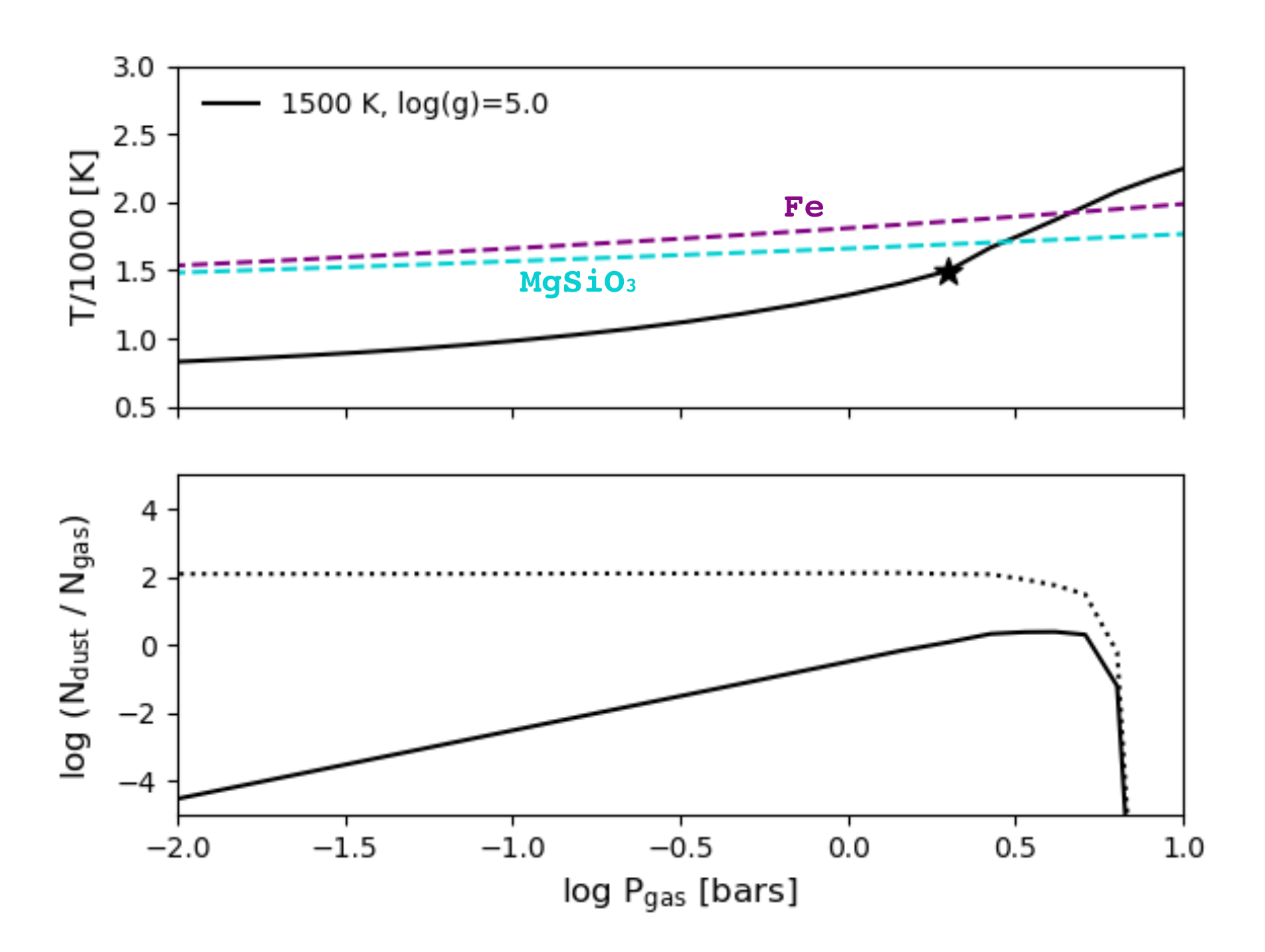
Figure 1: Top: Temperature-Pressure profile for cloudy atmosphere model with P_c=20 bars and a₀=0.25 $\mu$m. Condensation curves for iron and enstatite are shown. The star represents the location of the photosphere. Bottom: dust-to-gas ratio for pure equilibrium clouds (dotted line) and intermediate cloudy model (solid line).

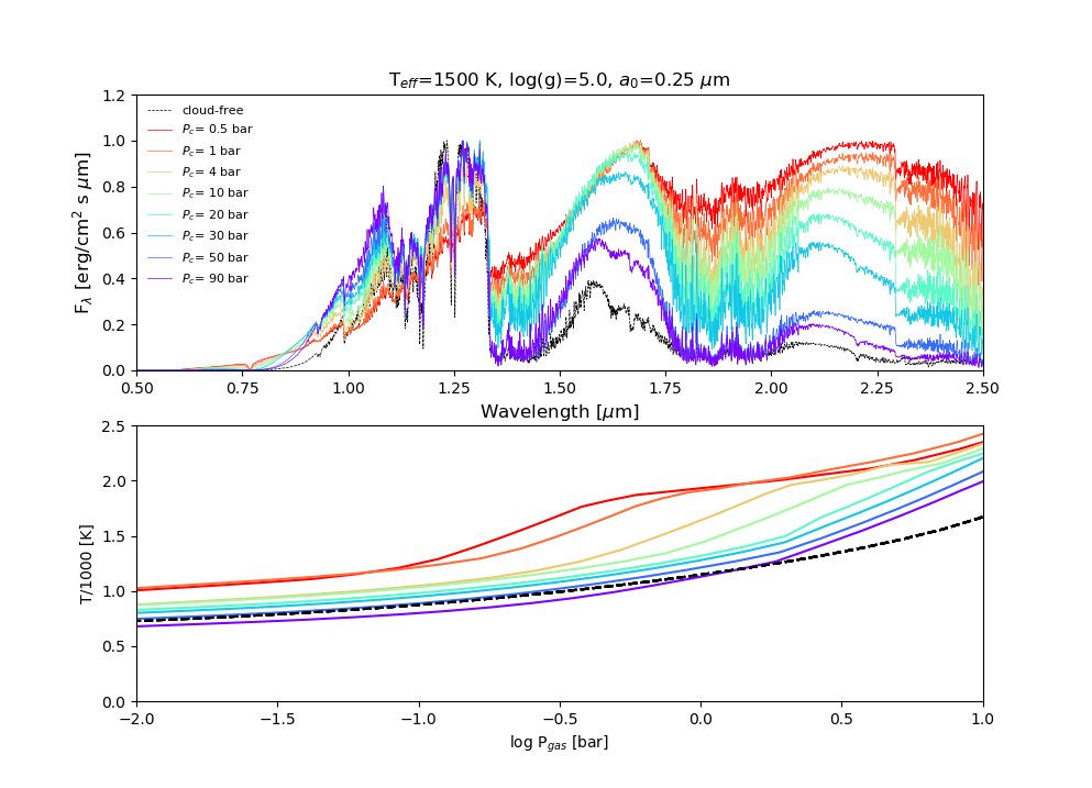
Figure 2: Comparison between model spectra and T-P profiles when cloud pressure, P_c, is varied. A cloud-free model is provided in black. Spectra were normalized and convolved with a Gaussian of FWHM$\approx$12 Å for clarity. All parameters are held constant except for cloud pressure.

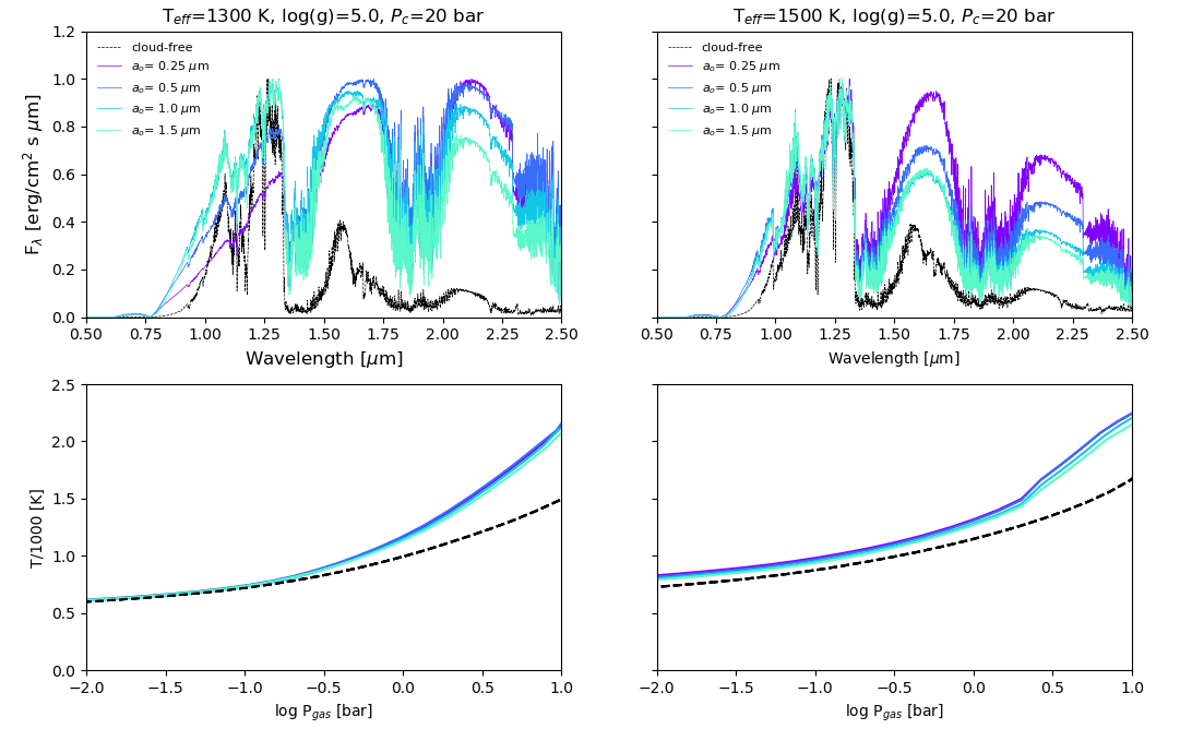
Figure 3: Comparison between model spectra and T-P profiles when mean grain size is varied. A cloud-free model is provided in black. Normalized spectra are shown for two effective temperatures. Spectra are convolved with a Gaussian of FWHM$\approx$12 Å for clarity. All parameters held constant except for grain size in each panel.

5 Results

5.1 Grid Fitting

We fit resolved photometry to model grids to better understand the nature of clouds in substellar atmospheres spanning the L/T transition. Table 7 summarizes the grid properties and includes the new grids created specifically for this work, extending cloud properties across a broader range of pressures and incorporating models with smaller mean grain sizes. All models in the grid are solar metallicity with effective temperatures ranging from 800-2000 K and surface gravities of log(g)=3.0-5.5. The conservative range of our models is suitable for objects from early L through early T dwarfs (Kirkpatrick, 2005).

We calculate synthetic photometry for all models using HST and 2MASS filter transmission curves mentioned in Section 2. A best-fitting model is determined for each object using a $\chi^{2}$ fitting approach. We take the scale factor as

$$s=(R/D)^{2},$$ (3)

where R is the radius of the object to be fit, and D is 10 parsecs for absolute magnitude.

Table 7: Model Parameter Ranges

$T_{\mathrm{eff}}$	log(g)	Pc	a0	Increments
[K]	[cm $s^{-2}$]	[bar]	[$\mu$m]
800-2000	3.5-5.5	0.5, 1, 4	1	100 K; 0.5 in log(g)
800-2000	4.75, 5.0, 5.5	10, 20, 30	0.25, 0.5, 1	100 K
1700-2000	4.5-5.5	0.1, 0.5	0.25	100 K; 0.5 in log(g)

Table 8 shows the results of our model fitting. Models are allowed at the 68% confidence level by taking $\chi^{2}$ distributed with five degrees of freedom (the four atmosphere model parameters in Table 7 and the object’s radius, which is simultaneously fit). This includes all models with $\Delta\chi^{2}<$ 11.3. Listed first is the overall best-fitting model from the cloudy atmosphere grids. We then calculate the weighted mean parameters by

$$\bar{m}=\frac{\Sigma_{i}W_{i}m_{i}}{\Sigma_{i}W_{i}},$$ (4)

where the weight $W_{i}$ for each model $m_{i}$ is given by

$$W_{i}=H_{i}e^{-0.5\chi^{2}},$$ (5)

where $H_{i}$ is a scaling factor that accounts for the uneven spacing of some atmospheric parameters on the grid, down weighting regions of dense sampling and up weighting regions of coarse sampling in proportion to the amount of parameter space covered.

We used the same approach as Stone et al. (2016) to calculate uncertainties using sided variance estimates with

$$\sigma_{m}=\frac{\Sigma_{i}W_{i}(m_{i}-\bar{m})^{2}}{\Sigma_{i}W_{i}},$$ (6)

where the sum is calculated using parameters above (+) or below (-) the mean values. In cases where the edge of the grid boundary was approached, we report an upper/lower limit for our uncertainty.

Table 8: Model Atmosphere Fits

	Best Fit					Weighted Mean
Name	Teff	log(g)	RJup	Pc	a0	Teff	log(g)	RJup	Pc	a0
HD 130948B	1400	3.5	1.68	4	1.0	1903${}^{+97}_{-4}$	4.5${}^{+0.50}_{-1.0}$	1.04${}^{+0.27}_{-0.29}$	0.22${}^{+0.28}_{-0.12}$	$\leq$ 1.0
HD 130948C	1400	4.0	1.76	4	1.0	1808${}^{+92}_{-8}$	4.5${}^{+0.59}_{-1.0}$	1.03${}^{+0.16}_{-0.34}$	0.47${}^{+0.03}_{-0.67}$	$\leq$ 1.0
2MASS 0920+35A	1300	4.75	1.50	4	1.0	1517${}^{+331}_{-194}$	4.88${}^{+0.47}_{-0.72}$	1.41${}^{+0.34}_{-0.47}$	2.9${}^{+2.9}_{-2.6}$	0.70${}^{+0.30}_{-0.43}$
2MASS 1728+39A	1500	5.5	0.95	30	0.25	1487${}^{+29}_{-131}$	5.17${}^{+0.33}_{-0.32}$	0.97${}^{+0.13}_{-0.05}$	20${}^{+10}_{-9}$	0.26${}^{+0.68}_{-0.01}$
2MASS 1728+39B	1400	4.75	0.83	20	1.0	1420${}^{+100}_{-22}$	4.99${}^{+0.43}_{-0.83}$	0.89${}^{+0.06}_{-0.09}$	8${}^{+10}_{-5}$	0.93${}^{+0.07}_{-0.44}$
LHS2397aB	1300	4.75	0.95	30	1.0	1413${}^{+93}_{-102}$	4.84${}^{+0.23}_{-0.09}$	0.81${}^{+0.12}_{-0.11}$	23${}^{+7}_{-3}$	0.54${}^{+0.46}_{-0.27}$
2MASS 0850+10A	1800	5.5	0.56	10	0.25	1717${}^{+91}_{-207}$	5.08${}^{+0.42}_{-0.63}$	0.65${}^{+0.22}_{-0.10}$	7.2${}^{+4.2}_{-6.1}$	0.36${}^{+0.55}_{-0.11}$
2MASS 0850+10B	1500	5.5	0.74	20	0.25	1423${}^{+80}_{-277}$	5.3${}^{+0.20}_{-0.69}$	0.93${}^{+0.80}_{-0.18}$	14${}^{+10}_{-7}$	0.37${}^{+0.63}_{-0.12}$
SDSS 1021-03A	1700	5.0	0.50	30	0.25	1668${}^{+37}_{-97}$	4.92${}^{+0.09}_{-0.17}$	0.52${}^{+0.09}_{-0.03}$	28${}^{+20}_{-8}$	0.36${}^{+0.57}_{-0.11}$
SDSS 1021-03B	1700	4.75	0.36	30	1.0	1698${}^{+2}_{-98}$	$\leq$ 5.5	0.36${}^{+0.06}_{-0.02}$	$\geq$ 0.1	0.96${}^{+0.04}_{-0.57}$
2MASS 1534-29A	1700	5.5	0.38	30	0.25	1699${}^{+1}_{-99}$	$\geq$ 3.5	0.38${}^{+0.02}_{-0.01}$	24${}^{+7}_{-4}$	$\leq$ 1.0
2MASS 1534-29B	1700	5.5	0.32	20	0.25	1699${}^{+1}_{-99}$	$\geq$ 3.5	0.33 $\pm$ 0.01	21${}^{+9}_{-3}$	$\leq$ 1.0

Note. — Best-fitting grid models and weighted means with 2-$\sigma$ uncertainties are provided. Weighted mean fits for HD 130948BC use a fixed range for radius 0.8-1.2 R_Jup constrained by Saumon & Marley (2008) evolutionary models. Fits in the table for 2MASS 1728+39B exclude the F814W photometric point and are discussed further in Section 6.3.

The results of our analysis are shown in Figures 4 and 5 for our sample of objects. We plot the best-fit and weighted mean grid models for each object from Table 8. These fits highlight the role clouds play in the uncertainties of effective temperature, gravity, and radius when fitting cloudy model grids to photometric observations. Three objects, 2MASS 1728+39AB and LHS 2397aB, were fit well by the grid and had properties consistent with evolutionary models shown in Figures 4 (c) and 5 (a).

Our fit of five parameters to HD 130948BC is not adequately constrained by the three photometric points used here. To help guide our fitting in subsequent sections and approach a unique solution for these objects, we applied a prior on radius (0.8-1.2 R_Jup) from evolutionary models for the weighted mean fits in Table 8. The unconstrained best-fit model and weighted fit are provided in Figure 4 (a). This shows how two atmosphere models with very different effective temperatures, gravities, and cloud properties can match $JHK$ photometric observations well. The best fits plotted in purple are much cooler than expected for early L-type objects and approach non-physical radii ($\geq$ 1.5 $R_{\mathrm{Jup}}$).

We note a few other objects where the grid fits present tension: 2MASS 0850+10AB, 2MASS 0920+35A, SDSS 1021-03AB, 2MASS 1534-29AB. Without incorporating evolutionary constraints on radius for the aforementioned systems, models allowed at 2-$\sigma$ over or under-predict effective temperature expected for a given spectral type (Leggett et al., 2002; Nakajima et al., 2004) and can result in non-physical radii. We believe this may be influenced by an unresolved component for some objects (e.g., 2MASS 0850+10A), and the cloud parameter space used in our grids does not appear to be appropriate for early-to-mid T dwarfs (e.g., 2MASS 1534-29AB). Figure 4 shows the grid fits for 2MASS 0850+10AB, SDSS 1021-03AB, and 2MASS 1534-29AB are warmer ($T_{\mathrm{eff}}$ $\geq$ 1700 K) and approach smaller than expected radii ($\leq$ 0.70 $R_{\mathrm{Jup}}$) for objects of field age (Dupuy & Liu, 2017). Conversely, the model fits for 2MASS 0920+35A shown in Figure 5 have radii larger than expected ($\geq$ 1.4 $R_{\mathrm{Jup}}$) for mid-L dwarfs (Leggett et al., 2002; Nakajima et al., 2004).

Figure 4: Best-fit (purple) and weighted mean (cyan) atmosphere models from Table 8. We chose the closest available model from our grid to the mean parameters. Corresponding synthetic photometry is plotted in same color as model spectra. Surface gravity is in cm $s^{-2}$. Spectral types included are from Dupuy & Liu (2017).

Figure 5: Best-fit (purple) and weighted mean (cyan) atmosphere models from Table 8. Only the best fits are shown for SDSS 1021-03AB and 2MASS 1534-29AB because weighted mean parameters are similar. Surface gravity is in cm $s^{-2}$. Spectral types included are from Dupuy & Liu (2017)

6 Evolutionary Model Comparisons

The addition of cloud properties in atmosphere models can lead to further degeneracies in mass and radius resulting in good fits to photometric data but producing non-physical properties given what we know of brown dwarf physics. An effective way to evaluate the quality of atmosphere model fits is by comparing the results to the bulk properties from evolutionary model predictions. We use bolometric luminosity constrained from our grid fits combined with the measured masses (Dupuy & Liu, 2017; Konopacky et al., 2010) to derive evolutionary predictions. We derive evolutionary predictions using Saumon & Marley (2008) hybrid grids for mid-to-late L dwarfs in our sample and use the Cond grids from Baraffe et al. (2003) for T dwarfs with T_eff $\lesssim$ 1300 K. Evolutionary properties are given in Table 9 and individual systems are discussed below.

We take comparisons a step further by running additional atmosphere models using a fixed value for effective temperature, gravity, and radius from evolutionary predictions in Table 9. Holding evolutionary properties constant, we ran additional models around the best-fitting cloud properties determined from our grid fits in Section 5. The goal was to determine if our cloudy atmosphere models could fit data well and remain consistent with substellar evolutionary model predictions.

Because we know the masses for these binary systems, distinguishing between different atmospheric fits becomes more reliable. We are able to eliminate model fits that may represent the data well yet result in implied masses that deviate from empirical observations. Implied mass is calculated from surface gravity and radius for a given atmosphere model. All model fits for individual systems are discussed below.

Table 9: Evolutionary Model Predictions

	Primary					Secondary
System	MJup	log($L_{\mathrm{bol}}/L_{\odot}$)	Teff	RJup	log(g)	MJup	log(${L_{\mathrm{bol}}}/{L_{\odot}}$)	Teff	RJup	log(g)	Age(Gyr)
HD 130948BC	59$\pm$1	-3.85 $\pm$ 0.09	1916${}^{+94}_{-90}$	1.05 $\pm$ 0.02	5.12 $\pm$ 0.02	56${}^{+2}_{-1}$	-3.91 $\pm$ 0.05	1851${}^{+46}_{-45}$	1.05 $\pm$ 0.02	5.10${}^{+0.02}_{-0.03}$	0.42${}^{+0.06}_{-0.04}$
2MASS 0920+35AB	71${}^{+3}_{-4}$	-4.28 $\pm$ 0.05	1604${}^{+51}_{-52}$	0.91${}^{+0.03}_{-0.01}$	5.32${}^{+0.03}_{-0.04}$	58${}^{+9}_{-7}$	-4.70 $\pm$ 0.05	1260${}^{+57}_{-52}$	0.91 $\pm$ 0.04	5.24 $\pm$ 0.10	1.82${}^{+0.35}_{-0.18}$
2MASS 1728+39AB	71${}^{+1}_{-2}$	-4.37 $\pm$ 0.04	1536${}^{+30}_{-41}$	0.90${}^{+0.02}_{-0.01}$	5.34${}^{+0.01}_{-0.04}$	68${}^{+1}_{-4}$	-4.52 $\pm$ 0.06	1417${}^{+42}_{-58}$	0.89${}^{+0.03}_{-0.01}$	5.33${}^{+0.01}_{-0.05}$	2.82${}^{+0.42}_{-1.24}$
LHS 2397aAB	92$\pm$1	-3.34$\pm$0.04	2533${}^{+41}_{-40}$	1.07 $\pm$ 0.02	5.29 $\pm$ 0.01	67${}^{+1}_{-9}$	-4.62 $\pm$ 0.02	1342${}^{+10}_{-39}$	0.88${}^{+0.04}_{-0.01}$	5.33${}^{+0.01}_{-0.10}$	3.02${}^{+0.07}_{-1.47}$
2MASS 0850+10AB	28${}^{+4}_{-5}$	-4.49 $\pm$ 0.06	1272${}^{+58}_{-57}$	1.14${}^{+0.03}_{-0.05}$	4.72${}^{+0.11}_{-0.12}$	26${}^{+5}_{-4}$	-4.54 $\pm$ 0.09	1234${}^{+79}_{-77}$	1.15${}^{+0.03}_{-0.06}$	4.70${}^{+0.09}_{-0.11}$	0.25${}^{+0.13}_{-0.09}$
SDSS 1021-03AB	29 $\pm$ 4	-4.70 $\pm$ 0.05	1219${}^{+48}_{-47}$	1.00${}^{+0.04}_{-0.03}$	4.85${}^{+0.09}_{-0.08}$	23 $\pm$ 4	-4.99 $\pm$ 0.01	1023${}^{+20}_{-24}$	1.02${}^{+0.04}_{-0.03}$	4.74${}^{+0.08}_{-0.11}$	0.47${}^{+0.08}_{-0.15}$
2MASS 1534-29AB	52 $\pm$ 3	-4.94 $\pm$ 0.02	1157${}^{+21}_{-7}$	0.83${}^{+0.02}_{-0.01}$	5.27${}^{+0.03}_{-0.04}$	47 $\pm$ 3	-5.08 $\pm$ 0.02	1062${}^{+19}_{-9}$	0.85${}^{+0.01}_{-0.02}$	5.21 $\pm$ 0.04	2.40 $\pm$ 0.07

Note. — Evolutionary model-derived properties from Saumon & Marley (2008) hybrid grids. For the T dwarfs, SDSS 1021A+B and 2MASS 1534-29A+B, evolutionary properties are from Baraffe et al. (2003) COND grids. Luminosity for LHS 2397aA is from Dupuy & Liu (2017).

6.1 HD 130948B+C

The best grid fit for the HD 130948B+C system does not match evolutionary-derived properties. This is not surprising because previous work has shown discrepancies between atmosphere grids and evolutionary properties ($\pm$ 250 K) when only $J$, $H$, and $K$ photometry are used (Dupuy et al., 2009). Barman et al. (2011) and other groups find similar issues for directly imaged planets. Additionally, limited SED coverage for this system leads to several well-fit models given grid fits are formally under-constrained. However, by fixing effective temperature, gravity, and radius using evolutionary-derived values we can fit for two cloud parameters to arrive at a more reliable solution that is formally allowed.

In Figure 6 we show our previous weighted mean grid fit compared to our new evolutionary fit with fixed $T_{\mathrm{eff}}$, log(g), and $R_{\mathrm{Jup}}$. A good fit to the data can be achieved for HD 130948B with a higher cloud and $a_{0}$=0.25 $\micron$ grain size. The fits are nearly identical, but the grid fit with lower surface gravity is inconsistent with measured mass compared to the higher surface gravity model ($M_{\mathrm{Jup}}$=14.08 and 58.68, respectively). HD 130948C is slightly cooler than the B component yet fit well with the same type of cloud and grain size. Again, the lower surface gravity model can be ruled out by implied mass ($M_{\mathrm{Jup}}$=13.54). The new evolutionary fits presented here for both objects are consistent with recent atmospheric properties determined by Briesemeister et al. (2019) which included both $J$, $H$, and $K$ photometry with additional ALES L-band spectra from 2.9–4.1 $\mu$m. Our updated fits provide additional constraints on the cloud properties of early-to-mid L type dwarfs.

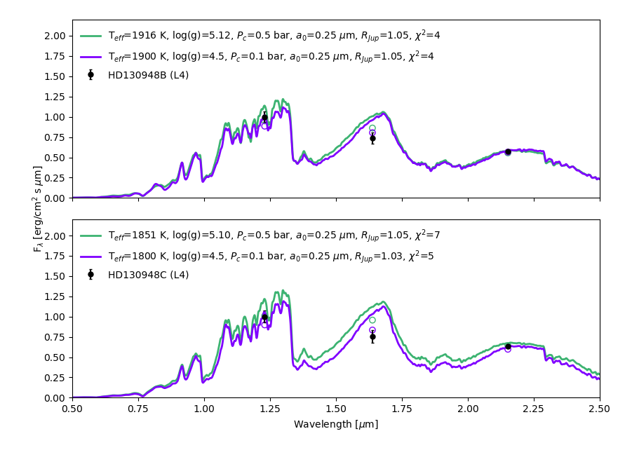
Figure 6: New evolutionary fit atmosphere models (green) compared to weighted mean grid fits (purple) for HD 130948B (top) and HD 130948C (bottom). Surface gravity is in cm $s^{-2}$.

6.2 2MASS 0850+10AB

We show our new evolutionary fits compared to our previous best-fitting grid model in Figure 7 for 2MASS 0850+10A and B. The initial grid fits significantly over-predicted temperature ($\approx$ 250-500 K) and gravity ($\approx$ 0.75 dex) while under-predicting radius compared to evolutionary predictions. Weighted mean parameters were consistent with evolutionary predictions for the secondary component but not for the primary (Table 8). Table 9 shows evolutionary predictions for this system have the lowest values of gravity (log(g) $\leq$ 4.75) for all the L dwarfs studied in this sample.

2MASS 0850+10A is fit well when bulk properties are fixed to evolutionary values and clouds include a 1 $\micron$ mean grain size. The warmer grid-based model ($T_{\mathrm{eff}}$=1800 K) can be ruled out by the larger implied mass ($M_{\mathrm{Jup}}$=40.04) and non-physical radius (0.56 $R_{\mathrm{Jup}}$) inconsistent with evolutionary models. Figure 7 shows how the grid fit for 2MASS 0850+10B compares to a cooler model with fixed evolutionary parameters. We can rule out the warmer 1500 K model because the implied mass (69.91 $M_{\mathrm{Jup}}$) is higher than the total measured mass of the entire system ($M_{\mathrm{tot}}$ = 54 $\pm$ 8 $M_{\mathrm{Jup}}$). For the $T_{\mathrm{eff}}$=1234 K model, the fit can be improved at $J$ band if the grain size is increased to 1 $\micron$, but this results in a poor fit to HST photometry near 0.75-1 $\micron$. A deeper cloud can also improve the $J$-band fit but reddens the $H$ and $K$ bands.

We believed the warmer, initial grid fit for this system, notably the primary, may have been caused by the spacing of our grid since evolutionary-predicted gravities for 2MASS 0850+10AB are near the edge of a boundary. To test this hypothesis and determine if the issue was indeed lack of sufficient grid coverage, we extended the segment of our grid that begins at log(g)=4.75 down to log(g)=4.5, including the same range of temperatures and cloud properties given in row two of Table 7. We then recalculated the grid fits for both A and B components. The best grid fit for 2MASS 0850+10A did not change with the addition of new lower gravity grid models. The weighted mean properties remained nearly identical to our previous findings and inconsistent with evolutionary predictions. The updated best grid fit for 2MASS 0850+10B resulted in an unusually cool model with a non-physical radius. Weighted mean parameters were again consistent with predictions from evolutionary models within the uncertainties, but the average gravity was still higher than expected (log(g)=5.25${}_{+0.25}^{-0.77}$).

Previous work has suggested 2MASS 0850+10A may be an unresolved binary. Burgasser et al. (2011) pointed out the object had unusually bright $J$ and $K$-band absolute magnitudes for a late L dwarf. Dupuy & Liu (2012, 2017) later determined with an updated system distance absolute magnitudes were similar to other L5-L7 dwarfs. Our HST photometry shows large differences in component brightnesses across multiple bands ($\Delta$F625W = 1.31 dex, $\Delta$F775W = 1.16 dex, $\Delta$F814W = 1.47 dex, and $\Delta$F850LP = 0.86 dex) hinting 2MASS 0850+10A might actually be composed of more than one object after all. The small total system mass of 54 $\pm$ 8 $M_{\mathrm{Jup}}$ implies 2MASS 0850+10A would be a pair of objects near the deuterium burning limit ($\approx$ 13.5 $M_{\mathrm{Jup}}$) with lower gravity (log(g)=4.3, $R_{\mathrm{Jup}}$=1.3) assuming the primary is an equal mass binary, and the B component is a more massive single object with higher gravity (log(g)=4.70, $R_{\mathrm{Jup}}$=1.15). The effective temperature in substellar evolutionary models can be quite flat for objects near 20 $M_{\mathrm{Jup}}$ at these ages due to clouds, and low-mass objects of similar effective temperatures have been known to look like mid-to-late L dwarfs (Barman et al., 2011). Fitting the A component as a binary would require more specialized atmosphere models.

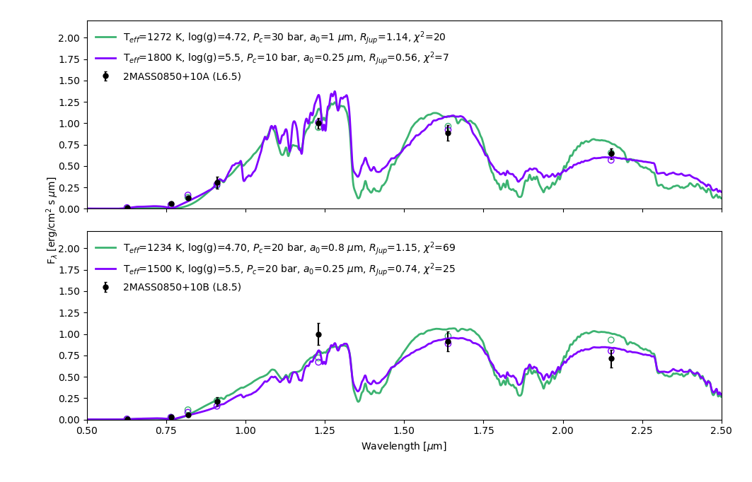
Figure 7: New evolutionary fit atmosphere models (green) compared to best grid fits (purple) for 2MASS 0850+10A (top) and 2MASS 0850+10B (bottom). Surface gravity is in cm $s^{-2}$.

6.3 2MASS 1728+39AB

The best grid fit for 2MASS 1728+39A is consistent with evolutionary predictions in temperature and radius but gravity is over-predicted resulting in an implied mass that is inconsistent with measured masses ($M_{\mathrm{Jup}}$=115.22). By fixing T_eff, log(g), and R_Jup to evolutionary predictions from Table 9 and adjusting the depth of the cloud, we are able to produce a good fit to the data shown in Figure 8. The 1536 K model has an implied mass consistent with measured mass ($M_{\mathrm{Jup}}$=71.54).

Fitting 2MASS 1728+39B was not as straightforward as fitting the A component. It was difficult to find a model fit that agreed reasonably well with the data simultaneously in both the F814W and F1042W bands even with fixed T_eff, log(g), and R_Jup to evolutionary predictions. The F814W data point was fit best by models with deeper clouds and 0.25 $\micron$ grains whereas the F1042W point preferred models with higher clouds and $\geq$ 1 $\micron$ grains. Figure 8 shows evolutionary model fits with both cloud preferences compared to our initial grid fit. The lower gravity 1400 K model can be excluded because its implied mass of $M_{\mathrm{Jup}}$=31.98 is less than half of the measured mass. For the remainder of this paper, we use the model fit that excludes the F814W photometric point as our preferred fit because it is more consistent with the majority of the photometric bands.

2MASS 1728+39AB is a flux reversal binary system, which may explain some of the difficulty finding an atmosphere model that fit in all bands. Several binary systems have been discovered with a secondary component brighter than the primary component in the 1.0-1.3 $\micron$ range (Gelino et al., 2014). In this system, the B component is brighter in the F1042W band ($\Delta_{A-B}$= 0.25 dex) but not in the $J$ or F814W bands. Looper et al. (2008a) explain the brightening could be the result of a cryptobinary, but it is often an intrinsic property of the object due to weather, unusual cloud properties, or changes in surface gravity. Surface gravity is unlikely to be the culprit because widely varying gravities requires different ages not expected for coeval binaries (Gelino et al., 2014). Our model fits suggest it may be due to differences in cloud location and particle sizes.

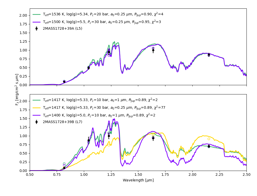
Figure 8: New evolutionary fit atmosphere models (green) compared to best grid fits (purple) for 2MASS 1728+39A (top) and 2MASS 1728+39B (bottom). Two fits for 2MASS 1728+39B are provided: one excluding the F814W photometric point (green) and one including it (gold). Surface gravity is in cm $s^{-2}$.

6.4 2MASS 0920+35AB

Dupuy & Liu (2017) suggest 2MASS 0920+35AB is a triple brown dwarf system given the large total mass of the system (187 $\pm$ 11 $M_{\mathrm{Jup}}$) with over half of the total system mass belonging to the fainter secondary (116${}^{+7}_{-8}$ $M_{\mathrm{Jup}}$). In order to obtain evolutionary predictions for the A component of this system, we follow the same approach as Dupuy & Liu (2017) and assume 2MASS 0920+35B is composed of two equal-mass, equal-luminosity components. These predictions are given in Table 9.

Figure 9 compares our best grid-fit model of 2MASS 0920+35A from Section 5 to a new model with fixed T_eff, log(g), and R_Jup from evolutionary predictions. We are able to produce a good fit to the data and remain consistent with evolutionary predictions if the B component is indeed a binary with two equal-mass, equal-luminosity components. We derive a younger age of the system at 1.82${}^{+0.35}_{-0.18}$ Gyr using SM08 evolutionary models, but our results are consistent within the uncertainties to the system age from Dupuy & Liu (2017) of 2.3${}^{+0.3}_{-0.4}$ Gyr.

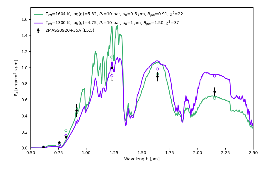
Figure 9: New evolutionary fit atmosphere model (green) compared to best grid fit (purple) for 2MASS 0920+35A. Surface gravity is in $s^{-2}$.

6.5 LHS2397aAB

We only studied the L dwarf companion in this system because the A component is a low-mass star and outside the temperature range of our grid fitting ($\geq$ 2000 K). Although the best grid-fitting model for LHS 2397aB was consistent in temperature and radius to evolutionary properties, the lower gravity resulted in an implied mass that was too small ($M_{\mathrm{Jup}}$=20.49). By fixing the bulk atmospheric properties of the object to evolutionary-derived properties from Table 9, we are able to get a good fit to the data with a new model show in Figure 10 that has an implied mass consistent with observations ($M_{\mathrm{Jup}}$=66.84).

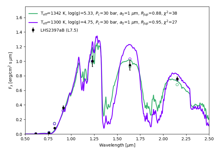
Figure 10: New evolutionary fit atmosphere model (green) compared to the best grid fit (purple) for LHS 2397aB. Surface gravity is in cm $s^{-2}$.

6.6 SDSS 1021-03AB

It became apparent our cloudy atmosphere grids did not sample enough of the parameter space in cloud pressure and grain size to accommodate early-to-mid T dwarfs, particularly at lower values of surface gravity near log(g)=4.75. $K$-band flux is sensitive to surface gravity (Saumon et al., 2012), and the cooler models in our grid more appropriate for T dwarfs predicted an overly red $H$ - $K$ color. We were able to obtain improved fits more appropriate for the SDSS 1021-03AB system by testing models outside the grid with larger grain sizes and deeper clouds.

The cloudy model fits presented here help to provide an upper limit to the location of clouds in T dwarf atmospheres, which are traditionally fit with cloud-free models (Baraffe et al., 2003). Figure 11 provides a comparison of the best grid models to new evolutionary-based models. The initial grid fits to the system have lower values of $\chi^{2}$ but significantly over-predicted temperature ($\geq$ 500 K) and under-predicted radius ($\leq$ 0.50 $R_{\mathrm{Jup}}$). Although the $J$-band flux is under-predicted by our evolutionary fit for SDSS 1021-03B, this model is still the preferred model based on mass and radius. If we allow the radius to vary, the fit at $J$-band can be improved using a model with a deeper cloud and larger grain size ($P_{c}$=100 bar, $a_{0}$=5 $\micron$) with a radius of 1.25 $R_{\mathrm{Jup}}$; however, this results in a 35 $M_{Jup}$ mass inconsistent with observations of 23 $\pm$ 4.

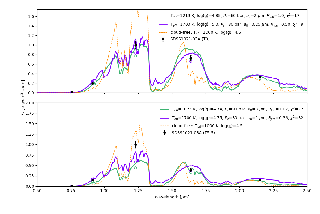
Figure 11: New evolutionary fit atmosphere models (green) compared to best grid fits (purple) for SDSS 1021-03A (top) and SDSS 1021-03B (bottom). Plotted in orange is a cloud-free model for comparison. Surface gravity is in cm $s^{-2}$.

6.7 2MASS 1534-29AB

Similar to the SDSS 1021-03AB system, the mid-T dwarfs in the 2MASS 1534-29AB system were not fit well by our cloudy atmosphere grids. Grid fits resulted in significantly over-predicted effective temperatures ($\geq$ 500 K) and small, non-physical radii ($\leq$ 0.40 $R_{\mathrm{Jup}}$) for both the A and B components.

Using cloud parameters informed from our evolutionary fits to the SDSS 1021-03AB system, we were able to test additional models and find more realistic fits for 2MASS 1534-29AB shown in Figure 12. The fits are greatly improved over the original grid-based models and help to provide upper limits to the cloud over cloud-free models.

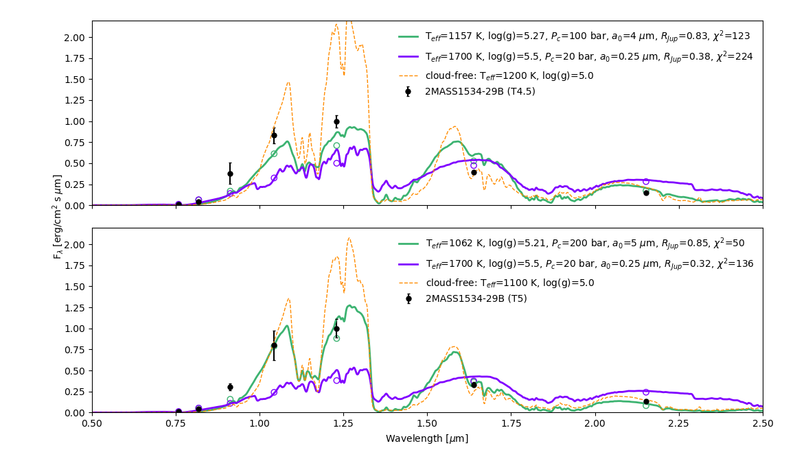
Figure 12: New evolutionary fit atmosphere models (green) compared to best grid fits (purple) for 2MASS 1534-29A (top) and 2MASS 1534-29B (bottom). Plotted in orange is a cloud-free model for comparison. Surface gravity is in cm $s^{-2}$.

7 Cloud Properties

Here we discuss detailed cloud properties from our best-fitting atmosphere models. For the remainder of the paper, we consider the best fits those constrained by evolutionary models in the previous section. Model parameters are summarized in Table 10. We also include the location of the photosphere, cloud location (top, base), cloud thickness, and peak gas-to-dust ratio in the table for reference. We adopt the approximate location of the spectrum-forming region (photosphere) where the atmospheric temperature equals the effective temperature. This location is also very close to where the Rosseland mean optical depth is $\approx$ 1.

The model cloud is composed of multiple layers of thermochemically permissible condensate species composed mostly of Fe and Mg-Si grains. Cloud opacity is determined from a heterogeneous mixture of these grains along with a number of minor contributors for which opacities are available rather than using a single grain type as representative of all cloud particles. We report the most abundant condensate species for each object in Table 11. While the table is representative of the composition at the cloud top layer, a gradient of condensates is present within the cloud.

Figure 13 illustrates how the cloud properties change in our sample for L to mid T-type dwarfs for T${}_{\mathrm{eff}}\approx$ 1900-1000 K. Cloud formation occurs higher in the atmosphere and shifts to deeper regions as effective temperature decreases. The peak dust-to-gas ratio shifts to deeper regions within the cloud for cooler objects as well. This trend emerges into two distinct clusters in the plot–one containing eight objects ($\approx$ L4-T5) and one containing four objects ($\approx$ L6-T5)–signifying a similar trend for high-gravity and low-gravity objects. It is worth noting all objects in our sample near $T_{\mathrm{eff}}$ $\leq$ 1400 K have detached convection zones from the radiative-convective boundary with a convective flux greater than 50% of the total flux. Isolated convection zones can emerge as temperatures decrease. These detached convection zones are a result of localized changes to the temperature gradient caused by the cloud opacity. Similar zones, produced for the same reason, were discussed by Burrows et al. (2006). In addition to the effective temperature and gravity, the location and vertical extent of these zones are sensitive to the detailed cloud properties (e.g., composition, particle size, and cloud morphology) that determine a cloud’s contribution to the total opacity.

Sub-micron grains (0.25-0.50 $\micron$) were the most appropriate for L4-L5.5 spectral types with temperatures of $\approx$1900-1500 K and high surface gravities (log(g) $\geq$ 5.0) and one lower gravity (log(g) $\leq$ 5.0) L8.5 dwarf. Previous work found comparable grain sizes for L dwarfs using a single grain type such as 0.4-0.6 $\micron$ for corundum and enstatite grains (Marocco et al., 2014), 0.15-0.3 $\micron$ for iron grains (Marocco et al., 2014), and a mean grain size of 0.15-0.35 $\micron$ using forsterite grains (Hiranaka et al., 2016). Rotational modulations have also suggested hazes present in L dwarf atmospheres have characteristic grain sizes of $\approx$0.28-0.4 $\micron$ (Lew et al., 2016).

Larger grain sizes ($\geq$ 1 $\micron$) were required for most spectral types later than L6.5-L7 with effective temperatures near 1400 K and cooler. The coolest and latest type objects in our sample required the largest grain sizes (2-5 $\micron$). Similarly, Zhou et al. (2018) found characteristic condensate particle sizes grew for later L types ($\geq$ L8) with larger mean grain sizes required to match observations (a₀ $\geq$ 1.0 $\mu$m).

We compare our modelled objects to the cooling and color evolution of brown dwarfs across the L/T transition using Saumon & Marley (2008) hybrid evolution models in Figure 14. Objects redder than the track were best represented by the smallest grain sizes, whereas objects bluer than the track where those that required the largest grain sizes. Reddened L dwarfs in the L5-L7.5 range can be an important indicator of youth in brown dwarfs, or the redder colors can be indicative of excess dust and clouds in the photosphere (Kirkpatrick, 2005; Filippazzo et al., 2015; Faherty et al., 2012). The reddest object in our sample, 2MASS 1728+39A, is a mid-L dwarf slightly redder than average ($J$ - $K_{s}$ = 2.07), which we believe is due to excess dust and a small cloud particle size.

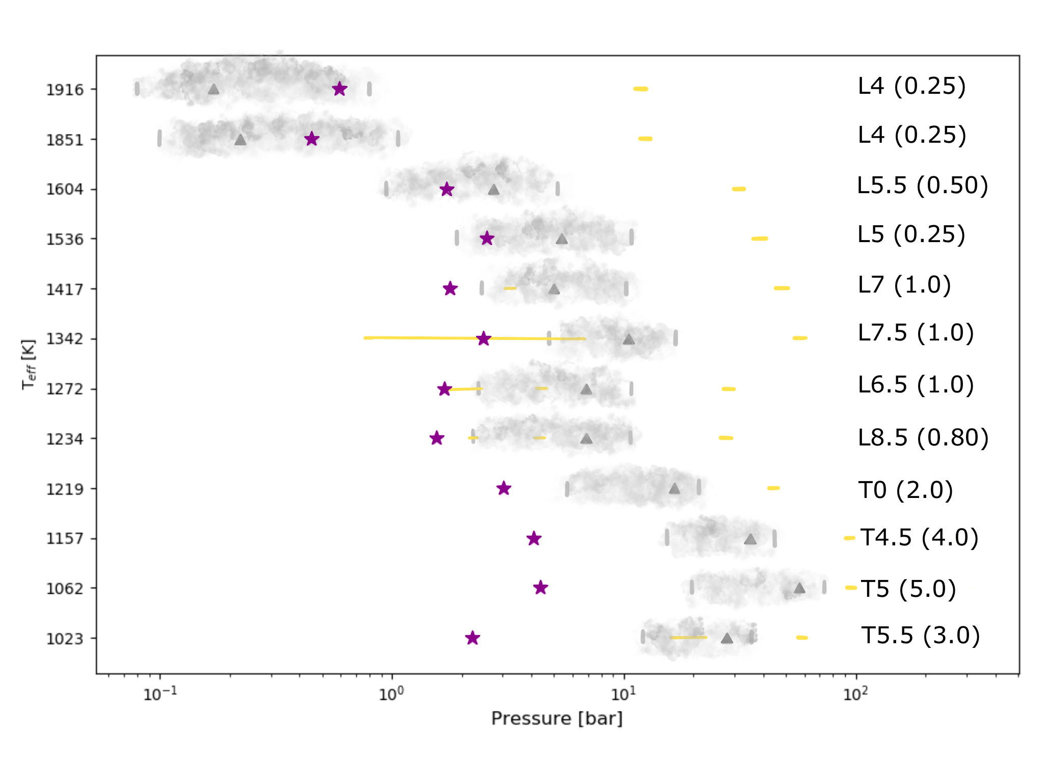
Figure 13: Summary of best-fit evolutionary model cloud progression organized by decreasing effective temperature with the warmest objects at the top. The photosphere for each model atmosphere is represented by a star. The cloud top and cloud base are denoted by light grey lines. The peak dust-to-gas ratio is represented by a grey triangle. Regions with a yellow line are indicative of convection with the right-most dash always indicating the radiative-convective boundary. Yellow regions to the left of the this boundary highlight a detached convection zone (F_conv/F_tot $\geq$ 50 %). Spectral type and the model’s mean grain size in $\micron$ is included on the right-hand side of the plot for reference.

Table 10: Summary of Evolutionary Constrained Cloud Properties

Object	Teff	log(g)	a0	Pc	Photosphere	Cloud Base	Cloud Top	Peak Dust	Hp	SpT
HD 130948B	1916	5.12	0.25	0.5	0.59	0.80	0.08	0.17	1.93	L4 $\pm$ 1
HD 130948C	1851	5.10	0.25	0.5	0.45	1.07	0.10	0.22	2.58	L4 $\pm$ 1
2MASS 0920+35A	1604	5.32	0.50	10	1.72	5.21	0.94	2.74	2.14	L5.5 $\pm$ 1
2MASS 1728+39A	1536	5.34	0.25	20	2.57	10.8	1.89	5.37	2.16	L5 $\pm$ 1
2MASS 1728+39B	1417	5.33	1.0	10	1.78	10.2	2.45	5.00	1.90	L7 $\pm$ 1
LHS2397aB	1342	5.33	1.0	30	2.49	16.7	4.79	10.5	1.53	L7.5 $\pm$ 1
2MASS 0850+10A	1272	4.72	1.0	30	1.68	10.8	2.37	6.90	1.84	L6.5 $\pm$ 1
2MASS 0850+10B	1234	4.70	0.8	20	1.56	10.7	2.24	6.84	1.90	L8.5 $\pm$ 1
SDSS 1021-03A	1219	4.85	2.0	60	3.04	21.0	5.67	16.5	1.57	T0 $\pm$ 1
2MASS 1534-29A	1157	5.27	4.0	100	4.06	44.6	15.4	34.9	1.30	T4.5 $\pm$ 1
2MASS 1534-29B	1062	5.21	5.0	200	4.35	73.6	19.6	57.2	1.48	T5 $\pm$ 1
SDSS 1021-03B	1023	4.74	3.0	90	2.21	35.4	12.1	27.8	1.26	T5.5 $\pm$ 1

Note. — Detailed model cloud properties for best evolutionary-derived atmosphere model fits from Section 6. Cloud properties are given in bars. H_p is the cloud thickness in pressure scale height. Spectral types listed are from Dupuy & Liu (2017).

Table 11: Most Abundant Condensates in Cloud Top Layer

Object	Condensates
HD 130948B	Fe (48%) — MgSiO3, Mg2SiO4, MgO, SiO2 (52%)
HD 130948C	Fe (49%) — MgSiO3, MgO, Mg2SiO4, SiO2 (51%)
2MASS 0920+35A	Fe (48%) — MgSiO3, Mg2SiO4, MgO, SiO2 (52%)
2MASS 1728+39A	Fe (49%) — MgSiO3, MgO, Mg2SiO4, SiO2 (51%)
2MASS 1728+39B	Fe (50%) — MgO, SiO2, Mg2SiO4, MgSiO3, MgAl2O4 (50%)
LHS2397aB	Fe (45%) — MgSiO3, MgO, SiO2, Mg2SiO4 (55%)
2MASS 0850+10A	Fe (49%) — MgSiO3, MgO, Mg2SiO4, SiO2 (51%)
2MASS 0850+10B	Fe (48%) — MgSiO3, Mg2SiO4, MgO, SiO2 (52%)
SDSS 1021-03A	Fe (47%) — MgSiO3, MgO, Mg2SiO4, SiO2 (53%)
2MASS 1534-29A	Fe (45%) — SiO2, MgO, Mg2SiO4, MgSiO3, MgAl2O4 (55%)
2MASS 1534-29B	Fe (46%) — SiO2, MgO, Mg2SiO4, MgSiO3, MgAl2O4 (54%)
SDSS 1021-03B	Fe (47%) — MgSiO3, MgO, SiO2, Mg2SiO4 (53%)

Note. — The most abundant dust species are listed for each object at the cloud top layer. Individual condensates species are in order from the most abundant to the least abundant and represent a combination of both solid and liquid phases. Percentages shown are for total iron grains and Mg-Si grains, respectively.

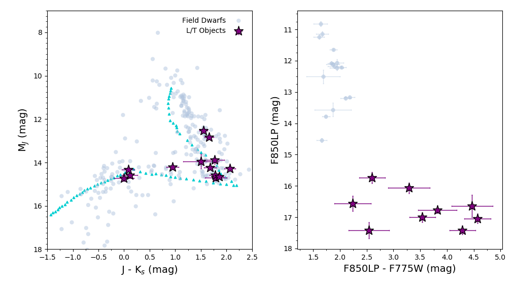
Figure 14: Color-magnitude diagrams in near-infrared and optical colors. Saumon & Marley (2008) hybrid evolutionary tracks are overplotted in turquoise triangles. Purple stars show the objects focused on in this paper. Filled light blue circles are low-mass field objects from Faherty et al. (2012) (left) and low-mass objects from Konopacky et al. (2010) (left and right). HST observations on right include both WFC3 and ACS filters.

8 Summary and Conclusion

Discrepancies between atmosphere and evolutionary model predictions play a significant role as different stages of condensate cloud evolution greatly influences the overall spectral shape. Previous grid comparisons have led to disagreements between atmosphere models and evolutionary predictions for substellar objects of known mass (e.g., Chabrier & Baraffe, 2000; Dupuy et al., 2014). We are able to produce atmosphere models that match evolutionary predictions for a sample of brown dwarfs ($\approx$ L4-T5) by allowing enough flexibility within the cloud properties.

Determining the bulk properties (e.g., effective temperature and gravity) of stellar and substellar mass objects is an important step along the way to making inferences about more specific properties, such as metallicity, or the relative abundances of key elements. These bulk properties are frequently estimated by comparing photometric or spectroscopic observations to model atmosphere predictions. For many objects such comparisons yield properties consistent with those of interior and evolution models that, at moderate to old ages, are considered reliable and less sensitive to model assumptions (Baraffe et al., 2002). Significant inconsistencies, however, can occur whenever condensate cloud formation greatly influences the overall spectral shape. This situation occurs, for example, across the L/T transition (Cushing et al., 2006) and for most young directly imaged companions (Metchev & Hillenbrand, 2006) where models with a range of temperatures, gravities, and cloud properties are capable of matching a single object’s near-IR SED equally well (Barman et al., 2011). Such ambiguity can often hinder the study of cloudy objects where mass and age are very uncertain.

In this paper we have studied a set of L/T transition ($T_{\mathrm{eff}}$ $\approx$ 1900-1000 K) brown dwarf binaries with measured masses, luminosities, and well-determined ages. For these objects comparisons to evolutionary models yield very precise estimates of the bulk properties. Overall, synthetic spectra from our cloudy atmosphere models matched spatially-resolved visible to near-IR photometry of each binary component reasonably well. The cloud parameters included in our grids appear to be most appropriate for L4-L8 field dwarfs with effective temperatures between 1900-1300 K and log(g) $\geq$ 5.0. The grid fits for these objects were the most consistent with our evolutionary-constrained atmosphere models.

With these atmosphere models we have determined a set of cloud properties across the L/T transition. The warmest objects in the sample ($\approx$1900-1500 K) were fit best by particles with mean grain sizes of 0.25-0.50 $\micron$, whereas objects cooler than 1500 K required larger mean grain sizes 0.80-5 $\micron$. Although the composition at the cloud top remained relatively close to an equal split between Fe and Mg-Si grains for the majority of objects, the overall location of the cloud top shifted to deeper regions within the atmosphere as objects cooled in effective temperature. Near 1400 K clouds began to disappear below the photosphere, which agrees with previous findings (Saumon & Marley, 2008; Marley et al., 2010).

There was some disagreement between our grid-based atmosphere models and the evolutionary-constrained atmosphere models for lower-gravity objects (log(g) $\leq$ 5.0) and the latest T dwarfs included in the sample (T4.5-T5.5; T_eff $\leq$ 1200 K). Our grid-based models tended to over-predict temperature, gravity, and under-predict radius. In addition to model-grid aspects (e.g., grid spacing and boundaries), unresolved binarity might play a role in some systems. For example 2MASS 0850+10A may be a pair of objects near the deuterium burning limit, rather than a single L-type brown dwarf, due to the large difference in brightness between A and B components, low total mass of the system, and mixed results from atmosphere model fitting. Giant exoplanets overlap with the range of effective temperatures of brown dwarfs (Faherty et al., 2016) and such objects (e.g., HR8799c) can resemble mid-L spectral types (Marois et al., 2010; Barman et al., 2011). Binarity is just one possibility and further study, both observationally and modeling, is warranted for this system.

SDSS 1021-03A is the earliest T dwarf in the sample, and evolutionary-constrained models preferred a deeper cloud (P_c=60 bar) and larger grain size ($>$ 1 $\micron$) slightly beyond the parameters in our atmosphere grids. Similarly, the later T4-T5 dwarfs (SDSS 1021-03B, 2MASS 1534-29A, 2MASS 1534-29B) required even deeper clouds (P_c=90-200 bar) and the largest grain sizes (3-5 $\micron$). Evolutionary-derived fits for these objects suggest our grids should be extended to include a larger range of cloud properties to accommodate early-to-mid T dwarfs and help constrain the limits of homogeneous cloud models for the coolest objects. We observe that condensate growth becomes more important near late-L types, leading to preferred model fits with larger mean grain sizes for T dwarfs. Other work has successfully reproduced T dwarf photometry using thin sulfide clouds (Morley et al., 2012) and inhomogeneous cloud cover with low temperature condensates (Na₂S, KCl) (Charnay et al., 2018). Near T_eff $\approx$ 1000 K cloud-free models may be a better fit to our data; however, this is the same regime in low-gravity objects where sulfide clouds appear while iron and silicate clouds are simultaneous disappearing (Morley et al., 2012; Charnay et al., 2018). A more diverse grid for these objects will be beneficial in order to untangle the relationship between condensate growth, cloud composition, and surface gravity.

Rapid color changes across the L/T transition have been interpreted as the result of patchy clouds or holes in the cloud deck (Burrows et al., 2003; Ackerman & Marley, 2001; Marley et al., 2010), a sudden collapse of the cloud deck (Tsuji & Nakajima, 2003), or an increase in sedimentation efficiency of clouds (Knapp et al., 2004). By parameterizing the sedimentation efficiency of dust particles to regulate the influence of cloud opacity on the model spectrum, one can reproduce the L/T transition (Saumon & Marley, 2008; Stephens et al., 2009). We are able to reproduce photometric changes across the L/T transition in a similar fashion by parameterizing the vertical extent and mean grain size of a uniform cloud. However, we cannot rule out the existence of patchy clouds in this sample of objects despite our homogeneous cloudy model fits because the presence of cloud holes is very subtle across the near-infrared part of the spectrum for L/T transition objects (Marley et al., 2010; Apai et al., 2013).

Other groups use a more complex treatment of grain nucleation, growth, evaporation, and/or drift. Work from Helling et al. (2008b, a) resulted in mean cloud particle sizes that increased as a function of atmospheric depth, with small particles ($\approx$ 0.01 $\micron$) in high atmospheric layers with a narrow grain size distribution that broadened to larger particle sizes ($\approx$ 100 $\micron$) and grain size distributions near the cloud base. Charnay et al. (2018) was able to reproduce the spread of near-IR colors across the L/T transition and those observed in reddened low-gravity objects by computing cloud particle radii estimated from simple microphysics. Our models use a constant grain size distribution with cloud height, but similar to more complex treatment of grains, the peak dust-to-gas ratio sinks to deeper regions within the atmosphere, eventually below observable layers.

It has been hinted at that grain size increases as objects cool across the L/T transition (Zhou et al., 2018; Knapp et al., 2004). Burrows et al. (2006) used models with homogeneous forsterite grains with sizes of 3, 10, 30, and 100 $\micron$ and identified that atmospheres with larger particles resulted in stronger $J$-band fluxes near 1400-1500 K due to the natural deepening of the cloud position in the model atmospheres. We observe something similar in our grid models across a smaller range of particle sizes (0.25-1 $\micron$) for our heterogeneous grains. Figure 3 shows $J$-band flux is greater for the largest grain sizes at 1300 K whereas $J$-band fluxes are similar at 1500 K regardless of grain size. A physical mechanism responsible for this trend in increasing grain size is not well understood. At cooler effective temperatures, it has been suggested that a larger supply of condensate vapor near the base of the cloud could result in runaway particle growth for cooler objects (Gao et al., 2018).

Photometry has limited sensitivity; therefore, future steps will be to improve atmospheric constraints with resolved spectroscopy. Cloud location, mean grain size, surface gravity, and metallicity impact our understanding substellar atmospheres as a function of temperature. Decoupling the degeneracies between these interwoven features is essential to explain observations of objects, particularly across the L/T transition. This work provides valuable insight into the complex evolution of cloud opacity for a range of well-studied brown dwarf binaries. Ideally, the goal is to be able to construct reliable atmosphere models that can account for the drastic color change and physical properties of substellar objects without a reliance on evolutionary models to infer the properties of individual objects. We plan to extend our cloudy grids to both lower and higher cloud top pressures with additional grain sizes to accommodate the earliest and latest spectral types. Additional exploration of cloud properties is warranted for the warmest and coolest objects for binaries where our atmosphere grids lacked coverage.

Future work would greatly benefit from additional observations, especially at the shortest wavelength portion of the SED. Photometric bands near 0.8-1 $\micron$ appear important when investigating flux reversal binary systems and provide insight to differing grain size preferences at optical and near-infrared wavelengths. The next generation of telescopes with higher sensitivity and wavelength coverage will be essential in providing high-quality spectra required to fine tune cloud parameters and address lingering inconsistencies, such as broad, continuous wavelength coverage from the James Webb Space Telescope’s NIRSpec instrument (0.6-5.3 $\micron$). Furthermore, variability has been detected in brown dwarfs at the transition region (Radigan, 2014) and will be an important factor for cloud formation and evolution going forward. Rotation-modulated spectral variations will be a key approach toward a more in-depth grasp of the evolving cloud structure in low-mass objects (Apai et al., 2013, 2017). Understanding the relationship between grain size distribution and effective temperature will require a multidimensional approach to grain kinetics and growth connected to convective cloud structure. Atmospheric retrieval results can be compared to those of self-consistent models to better understand the nature of discrepancies (e.g., heterogeneous cloud layers, particle sizes, cloud composition, haze layers). Relatively few brown dwarfs spanning the L/T transition have known masses, and the release of future Gaia data will increase parallax precision by 30% (Collaboration et al., 2020). Objects with independently constrained properties from dynamical mass and luminosity measurements are the strongest candidates for future model comparisons.

9 Acknowledgements

L. S. B. is extremely grateful for Kyle Pearson and many helpful discussions of this work. We would also like to thank the anonymous referee for a constructive report. Support for program 11605 was provided by NASA through a grant from the Space Telescope Science Institute, which is operated by the Associations of Universities for Research in Astronomy, incorporated under NASA contract NAS5-26555. This work was also supported by NSF grants 1405505 and 1614492. Material presented in this work is supported by the National Aeronautics and Space Administration under Grants/Contracts/Agreements No.NNX17AB63G issued through the Astrophysics Division of the Science Mission Directorate. This research makes use of data products from 2MASS, a joint project of the University of Massachusetts and the Infrared Processing and Analysis Center/California Institute of Technology, funded by the National Aeronautics and Space Administration and the National Science Foundation. Some of the data presented herein were also obtained at the W. M. Keck Observatory, which is operated as a scientific partnership among the California Institute of Technology, the University of California, and the National Aeronautics and Space Administration. The Observatory was made possible by the generous financial support of the W. M. Keck Foundation. The authors also recognize and acknowledge the very significant cultural role and reverence that the summit of Mauna Kea has always had within the indigenous Hawaiian community. We are most fortunate to have the opportunity to conduct observations from this mountain. Additionally, this research has benefited from the SpeX Prism Library, maintained by Adam Burgasser at http://www.browndwarfs.org/spexprism.

References

- Ackerman & Marley (2001) Ackerman, A. S., & Marley, M. S. 2001, The Astrophysical Journal, 556, 872, doi: 10.1086/321540
- Allard (2013) Allard, F. 2013, Proceedings of the International Astronomical Union, 8, 271, doi: 10.1017/S1743921313008545
- Allard et al. (2001) Allard, F., Hauschildt, P. H., Alexander, D. R., Tamanai, A., & Schweitzer, A. 2001, The Astrophysical Journal, 556, 357, doi: 10.1086/321547
- Anderson & King (2006) Anderson, J., & King, I. R. 2006, PSFs, Photometry, and Astronomy for the ACS/WFC, Tech. rep., STsCI. http://adsabs.harvard.edu/cgi-bin/nph-data_query?bibcode=2006acs..rept....1A&link_type=ABSTRACT%5Cnpapers://fedb1a86-f693-4042-a040-86e952d868c2/Paper/p1757
- Apai et al. (2013) Apai, D., Radigan, J., Buenzli, E., et al. 2013, Astrophysical Journal, 768, doi: 10.1088/0004-637X/768/2/121
- Apai et al. (2017) Apai, D., Karalidi, T., Marley, M. S., et al. 2017, Science, 357, 683, doi: 10.1126/science.aam9848
- Baraffe et al. (2002) Baraffe, I., Chabrier, G., Allard, F., & Hauschildt, P. H. 2002, Astronomy and Astrophysics, 382, 563, doi: 10.1051/0004-6361:20011638
- Baraffe et al. (2003) Baraffe, I., Chabrier, G., Barman, T. S., Allard, F., & Hauschildt, P. H. 2003, Astronomy and Astrophysics, 402, 701, doi: 10.1051/0004-6361:20030252
- Barman et al. (2015) Barman, T. S., Konopacky, Q. M., Macintosh, B., & Marois, C. 2015, Astrophysical Journal, 804, 1, doi: 10.1088/0004-637X/804/1/61
- Barman et al. (2011) Barman, T. S., MacIntosh, B., Konopacky, Q. M., & Marois, C. 2011, Astrophysical Journal Letters, 735, 2, doi: 10.1088/2041-8205/735/2/L39
- Baron & Hauschildt (2007) Baron, E., & Hauschildt, P. H. 2007, Astronomy and Astrophysics, 468, 255, doi: 10.1051/0004-6361:20066755
- Briesemeister et al. (2019) Briesemeister, Z. W., Skemer, A. J., Stone, J. M., et al. 2019, The Astronomical Journal, 157, 244, doi: 10.3847/1538-3881/ab1901
- Burgasser et al. (2008a) Burgasser, A., Liu, M. C., Ireland, M. J., Cruz, K. L., & Dupuy, T. J. 2008a, Astrophysical Journal, 681, 579
- Burgasser (2014) Burgasser, A. J. 2014, in Astronomical Society of India Conference Series, Vol. 11, Astronomical Society of India Conference Series, 7–16. https://arxiv.org/abs/1406.4887
- Burgasser et al. (2011) Burgasser, A. J., Bardalez-Gagliuffi, D. C., & Gizis, J. E. 2011, Astronomical Journal, 141, doi: 10.1088/0004-6256/141/3/70
- Burgasser et al. (2010) Burgasser, A. J., Cruz, K. L., Cushing, M., et al. 2010, Astrophysical Journal, 710, 1142, doi: 10.1088/0004-637X/710/2/1142
- Burgasser et al. (2006) Burgasser, A. J., Geballe, T. R., Leggett, S. K., Kirkpatrick, J. D., & Golimowski, D. A. 2006, The Astrophysical Journal, 637, 1067, doi: 10.1086/498563
- Burgasser et al. (2003) Burgasser, A. J., Kirkpatrick, J. D., Liebert, J., & Burrows, A. 2003, The Astrophysical Journal, 594, 510, doi: 10.1086/376756
- Burgasser et al. (2008b) Burgasser, A. J., Looper, D. L., Kirkpatrick, J. D., Cruz, K. L., & Swift, B. J. 2008b, The Astrophysical Journal, 674, 451, doi: 10.1086/524726
- Burgasser et al. (2007) Burgasser, A. J., Looper, D. L., Kirkpatrick, J. D., & Liu, M. C. 2007, The Astrophysical Journal, 658, 557, doi: 10.1086/511518
- Burgasser & McElwain (2006) Burgasser, A. J., & McElwain, M. W. 2006, The Astronomical Journal, 131, 1007, doi: 10.1086/499042
- Burgasser et al. (2004) Burgasser, A. J., McElwain, M. W., Kirkpatrick, J. D., et al. 2004, The Astronomical Journal, 127, 2856, doi: 10.1086/383549
- Burrows et al. (2001) Burrows, A., Hubbard, W. B., Lunine, J. I., & Liebert, J. 2001, Reviews of Modern Physics, 73, 719, doi: 10.1103/RevModPhys.73.719
- Burrows et al. (2006) Burrows, A., Sudarsky, D., & Hubeny, I. 2006, The Astrophysical Journal, 640, 1063
- Burrows et al. (2003) Burrows, A., Sudarsky, D., & Lunine, J. I. 2003, The Astrophysical Journal, 596, 587, doi: 10.1086/377709
- Chabrier & Baraffe (2000) Chabrier, G., & Baraffe, I. 2000, Annual Review of Astronomy and Astrophysics, 38, 337
- Charnay et al. (2018) Charnay, B., Bézard, B., Baudino, J. L., et al. 2018, The Astrophysical Journal, 854, 172, doi: 10.3847/1538-4357/aaac7d
- Chiu et al. (2006) Chiu, K., Fan, X., Leggett, S. K., et al. 2006, The Astronomical Journal, 131, 2722, doi: 10.1086/501431
- Collaboration et al. (2018) Collaboration, G., Brown, A. G. A., Vallenari, A., et al. 2018, Astronomy and Astrophysics, 616, 1
- Collaboration et al. (2020) Collaboration, G., Brown, A., Vallenari, A., et al. 2020, Astronomy and Astrophysics Astrophysics, 61, 1. https://arxiv.org/abs/2012.01533v1
- Crepp et al. (2018) Crepp, J. R., Principe, D. A., Wolff, S., et al. 2018, arXiv, 853, 192, doi: 10.3847/1538-4357/aaa2fd
- Cruz et al. (2004) Cruz, K. L., Burgasser, A. J., Reid, I. N., & Liebert, J. 2004, The Astrophysical Journal, 604, L61
- Cruz et al. (2009) Cruz, K. L., Kirkpatrick, J. D., & Burgasser, A. J. 2009, Astronomical Journal, 137, 3345, doi: 10.1088/0004-6256/137/2/3345
- Cruz et al. (2017) Cruz, K. L., Núñez, A., Burgasser, A. J., et al. 2017, The Astronomical Journal, 155, 34, doi: 10.3847/1538-3881/aa9d8a
- Cushing et al. (2010) Cushing, M. C., Saumon, D., & Marley, M. S. 2010, Astronomical Journal, 140, 1428, doi: 10.1088/0004-6256/140/5/1428
- Cushing et al. (2006) Cushing, M. C., Roellig, T. L., Marley, M. S., et al. 2006, The Astrophysical Journal, 648, 614, doi: 10.1086/505637
- Cushing et al. (2008) Cushing, M. C., Marley, M. S., Saumon, D., et al. 2008, The Astrophysical Journal, 678, 1372, doi: 10.1086/526489
- Cutri et al. (2003) Cutri, R. M., Skrutskie, M. F., van Dyk, S., et al. 2003, 2MASS All Sky Catalog of point sources, Tech. rep., The IRSA 2MASS All-Sky Point Source Catalog, NASA/IPAC Infrared Science Archive. https://ui.adsabs.harvard.edu/#abs/2003tmc..book.....C/abstract
- Diolaiti et al. (2000) Diolaiti, E., Bendinelli, O., Bonaccini, D., et al. 2000, Astronomy and Astrophysics Supplement Series, 147, 335, doi: 10.1051/aas:2000305
- Dupuy & Liu (2012) Dupuy, T. J., & Liu, M. C. 2012, Astrophysical Journal, Supplement Series, 201, doi: 10.1088/0067-0049/201/2/19
- Dupuy & Liu (2017) —. 2017, The Astrophysical Journal Supplement Series, 231, 15, doi: 10.3847/1538-4365/aa5e4c
- Dupuy et al. (2009) Dupuy, T. J., Liu, M. C., & Bowler, B. P. 2009, Astrophysical Journal, 706, 328, doi: 10.1088/0004-637X/706/1/328
- Dupuy et al. (2014) Dupuy, T. J., Liu, M. C., & Ireland, M. J. 2014, Astrophysical Journal, 790, doi: 10.1088/0004-637X/790/2/133
- Faherty et al. (2012) Faherty, J. K., Burgasser, A. J., Walter, F. M., et al. 2012, Astrophysical Journal, 752, doi: 10.1088/0004-637X/752/1/56
- Faherty et al. (2016) Faherty, J. K., Riedel, A. R., Cruz, K. L., et al. 2016, The Astrophysical Journal Supplement Series, 225, 10, doi: 10.3847/0067-0049/225/1/10
- Ferguson et al. (2005) Ferguson, J. W., Alexander, D. R., Allard, F., et al. 2005, The Astrophysical Journal, 623, 585, doi: 10.1086/428642
- Filippazzo et al. (2015) Filippazzo, J. C., Rice, E. L., Faherty, J., et al. 2015, Astrophysical Journal, 810, doi: 10.1088/0004-637X/810/2/158
- Freedman et al. (2008) Freedman, R. S., Marley, M. S., & Lodders, K. 2008, The Astrophysical Journal Supplement Series, 174, 504, doi: 10.1086/521793
- Gao et al. (2018) Gao, P., Marley, M. S., & Ackerman, A. S. 2018, The Astrophysical Journal, 855, 86, doi: 10.3847/1538-4357/aab0a1
- Gelino et al. (2014) Gelino, C. R., Smart, R. L., Marocco, F., et al. 2014, Astronomical Journal, 148, 4, doi: 10.1088/0004-6256/148/1/6
- Gennaro et al. (2019) Gennaro, M., Baggett, S., & Bajaj, V. 2019, A characterization of persistence at short times in the WFC3/IR detector. II, Tech. rep., STsCI. https://ui.adsabs.harvard.edu/#abs/2018wfc..rept....5G/abstract
- Gizis et al. (2012) Gizis, J. E., Faherty, J. K., Liu, M. C., et al. 2012, Astronomical Journal, 144, 1, doi: 10.1088/0004-6256/144/4/94
- Hauschildt (1993) Hauschildt, P. H. 1993, Journal of Quantitative Spectroscopy and Radiative Transfer, 50, 301, doi: https://doi.org/10.1016/0022-4073(93)90080-2
- Hauschildt et al. (1998) Hauschildt, P. H., Allard, F., & Baron, E. 1998, The Astrophysical Journal, 512, 377, doi: 10.1086/306745
- Hauschildt & Baron (2006) Hauschildt, P. H., & Baron, E. 2006, Astronomy and Astrophysics, 451, 273, doi: 10.1051/0004-6361:20053846
- Helling & Casewell (2014) Helling, C., & Casewell, S. 2014, Astronomy and Astrophysics Review, 22, 1, doi: 10.1007/s00159-014-0080-0
- Helling et al. (2008a) Helling, C., Woitke, P., & Thi, W. F. 2008a, Astronomy and Astrophysics, 485, 547, doi: 10.1051/0004-6361:20078220
- Helling et al. (2008b) Helling, C., Ackerman, A., Allard, F., et al. 2008b, Monthly Notices of the Royal Astronomical Society, 391, 1854, doi: 10.1111/j.1365-2966.2008.13991.x
- Hiranaka et al. (2016) Hiranaka, K., Cruz, K. L., Douglas, S. T., Marley, M. S., & Baldassare, V. F. 2016, The Astrophysical Journal, 830, 1, doi: 10.3847/0004-637X/830/2/96
- Kirkpatrick (2005) Kirkpatrick, J. D. 2005, Annual Review of Astronomy and Astrophysics, 43, 195, doi: 10.1146/annurev.astro.42.053102.134017
- Kirkpatrick et al. (2008) Kirkpatrick, J. D., Cruz, K. L., Barman, T. S., et al. 2008, The Astrophysical Journal, 689, 1295, doi: 10.1086/592768
- Kirkpatrick et al. (2010) Kirkpatrick, J. D., Looper, D. L., Burgasser, A. J., et al. 2010, Astrophysical Journal, Supplement Series, 190, 100, doi: 10.1088/0067-0049/190/1/100
- Knapp et al. (2004) Knapp, G. R., Leggett, S. K., Fan, X., et al. 2004, The Astrophysical Journal, 3553
- Konopacky et al. (2010) Konopacky, Q. M., Ghez, A. M., Barman, T. S., et al. 2010, Astrophysical Journal, 711, 1087, doi: 10.1088/0004-637X/711/2/1087
- Krist et al. (2011) Krist, J. E., Hook, R. N., & Stoehr, F. 2011, in Optical Modeling and Performance Predictions V, ed. M. A. Kahan, Vol. 8127, International Society for Optics and Photonics (SPIE), 166–181, doi: 10.1117/12.892762
- Lane et al. (2002) Lane, B. F., Osorio, M. R. Z., Britton, M. C., Martin, E. L., & Kulkarni, S. R. 2002, The Astrophysical Journal, 560, 390, doi: 10.1086/322506
- Leggett et al. (2002) Leggett, S. K., Golimowski, D. A., Fan, X., et al. 2002, The Astrophysical Journal, 564, 452, doi: 10.1086/324037
- Lew et al. (2016) Lew, B. W. P., Apai, D., Zhou, Y., et al. 2016, The Astrophysical Journal Letters, 829, 1, doi: 10.3847/2041-8205/829/2/L32
- Lew et al. (2020) Lew, B. W. P., Apai, D., Marley, M., et al. 2020, arXiv, doi: 10.3847/1538-4357/abb81d
- Liu et al. (2016) Liu, M. C., Dupuy, T. J., & Allers, K. N. 2016, The Astrophysical Journal, 833, 1, doi: 10.3847/1538-4357/833/1/96
- Liu et al. (2008) Liu, M. C., Dupuy, T. J., & Ireland, M. J. 2008, The Astrophysical Journal, 689, 436, doi: 10.1086/591837
- Lodders & Fegley (2002) Lodders, K., & Fegley, B. 2002, Icarus, 155, 393, doi: 10.1006/icar.2001.6740
- Looper et al. (2008a) Looper, D. L., Kirkpatrick, J. D., & Burgasser, A. J. 2008a, The Astronomical Journal, 134, 1162, doi: 10.1086/520645
- Looper et al. (2008b) Looper, D. L., Kirkpatrick, J. D., Cutri, R. M., et al. 2008b, The Astrophysical Journal, 686, 528, doi: 10.1086/591025
- Marley et al. (1999) Marley, M. S., Gelino, C., Stephens, D., Lunine, J. I., & Freedman, R. 1999, The Astrophysical Journal, 513, 879, doi: 10.1086/306881
- Marley & Robinson (2015) Marley, M. S., & Robinson, T. D. 2015, Annual Review of Astronomy and Astrophysics, 53, 279, doi: 10.1146/annurev-astro-082214-122522
- Marley et al. (2010) Marley, M. S., Saumon, D., & Goldblatt, C. 2010, Astrophysical Journal Letters, 723, 117, doi: 10.1088/2041-8205/723/1/L117
- Marley et al. (2002) Marley, M. S., Seager, S., Saumon, D., et al. 2002, The Astrophysical Journal, 568, 335, doi: 10.1086/338800
- Marocco et al. (2014) Marocco, F., Day-jones, A. C., Lucas, P. W., et al. 2014, Monthly Notices of the Royal Astronomical Society, 439, 372, doi: 10.1093/mnras/stt2463
- Marois et al. (2010) Marois, C., Zuckerman, B., Konopacky, Q. M., Macintosh, B., & Barman, T. 2010, Nature, 468, 1080, doi: 10.1038/nature09684
- McLean et al. (2003) McLean, I. S., McGovern, M. R., Burgasser, A. J., et al. 2003, The Astrophysical Journal, 596, 561, doi: 10.1086/377636
- Metchev & Hillenbrand (2006) Metchev, S. A., & Hillenbrand, L. A. 2006, The Astrophysical Journal, 651, 1166, doi: 10.1086/507836
- Miles et al. (2020) Miles, B. E., Skemer, A. J. I., Morley, C. V., et al. 2020, The Astronomical Journal, 160, 63, doi: 10.3847/1538-3881/ab9114
- Morley et al. (2012) Morley, C. V., Fortney, J. J., Marley, M. S., et al. 2012, Astrophysical Journal, 756, doi: 10.1088/0004-637X/756/2/172
- Nakajima et al. (2004) Nakajima, T., Tsuji, T., & Yanagisawa, K. 2004, The Astrophysical Journal, 607, 499, doi: 10.1086/383299
- Radigan (2014) Radigan, J. 2014, Astrophysical Journal, 797, doi: 10.1088/0004-637X/797/2/120
- Reid et al. (2006) Reid, I. N., Lewitus, E., Burgasser, A. J., & Cruz, K. L. 2006, The Astrophysical Journal, 639, 1114, doi: 10.1086/499484
- Saumon et al. (2012) Saumon, D., Bergeron, P., Lunine, J. I., Hubbard, W. B., & Burrows, A. 2012, The Astrophysical Journal, 424, 333
- Saumon & Marley (2008) Saumon, D., & Marley, M. S. 2008, The Astrophysical Journal, 689, 1327, doi: 10.1086/592734
- Schmidt et al. (2010) Schmidt, S. J., West, A. A., Burgasser, A. J., Bochanski, J. J., & Hawley, S. L. 2010, Astronomical Journal, 139, 1045, doi: 10.1088/0004-6256/139/3/1045
- Sharp & Burrows (2007) Sharp, C. M., & Burrows, A. 2007, The Astrophysical Journal Supplement Series, 168, 140, doi: 10.1086/508708
- Showman et al. (2018) Showman, A. P., Tan, X., & Zhang, X. 2018, The Astronomical Journal, 883, 4, doi: 10.3847/1538-4357/ab384a
- Stephens et al. (2009) Stephens, D. C., Leggett, S. K., Cushing, M. C., et al. 2009, Astrophysical Journal, 702, 154, doi: 10.1088/0004-637X/702/1/154
- Stone et al. (2016) Stone, J. M., Eisner, J., Skemer, A., et al. 2016, The Astrophysical Journal, 829, 39, doi: 10.3847/0004-637x/829/1/39
- Stone et al. (2020) Stone, J. M., Barman, T., Skemer, A. J., et al. 2020, The Astronomical Journal, 160, 11. https://arxiv.org/abs/2010.02928
- Tan & Showman (2019) Tan, X., & Showman, A. P. 2019, The Astrophysical Journal, 874, 111, doi: 10.3847/1538-4357/ab0c07
- Tan & Showman (2021a) —. 2021a, Monthly Notices of the Royal Astronomical Society, 502, 2198, doi: 10.1093/mnras/stab097
- Tan & Showman (2021b) —. 2021b, Monthly Notices of the Royal Astronomical Society, 502, 678, doi: 10.1093/mnras/stab060
- Tennyson & Yurchenko (2012) Tennyson, J., & Yurchenko, S. N. 2012, Monthly Notices of the Royal Astronomical Society, 425, 21, doi: 10.1111/j.1365-2966.2012.21440.x
- Tsuji & Nakajima (2003) Tsuji, T., & Nakajima, T. 2003, The Astrophysical Journal, 151
- Tsuji et al. (1996) Tsuji, T., Ohnaka, K., Aoki, W., & Nakajima, T. 1996, Astronomy and Astrophysics, 308, L29. https://arxiv.org/abs/arXiv:1011.1669v3
- Wood et al. (2019) Wood, C. M., Boyajian, T., von Braun, K., et al. 2019, The Astrophysical Journal, 873, 83, doi: 10.3847/1538-4357/aafe01
- Zhang & Showman (2014) Zhang, X., & Showman, A. P. 2014, Astrophysical Journal Letters, 788, 2, doi: 10.1088/2041-8205/788/1/L6
- Zhang et al. (2020) Zhang, Z., Liu, M. C., Marley, M. S., Line, M. R., & Best, W. M. 2020, arXiv, 1. https://arxiv.org/abs/2011.12294
- Zhou et al. (2018) Zhou, Y., Apai, D., Metchev, S., et al. 2018, The Astronomical Journal, 155, 132, doi: 10.3847/1538-3881/aaabbd