Numerical renormalization group-based approach to secular perturbation theory

Abstract

Perturbation theory is a crucial tool for many physical systems, when exact solutions are not available, or nonperturbative numerical solutions are intractable. Naive perturbation theory often fails on long timescales, leading to secularly growing solutions. These divergences have been treated with a variety of techniques, including the powerful dynamical renormalization group (DRG). Most of the existing DRG approaches rely on having analytic solutions up to some order in perturbation theory. However, sometimes the equations can only be solved numerically. We reformulate the DRG in the language of differential geometry, which allows us to apply it to numerical solutions of the background and perturbation equations. This formulation also enables us to use the DRG in systems with background parameter flows, and therefore, extend our results to any order in perturbation theory. As an example, we apply this method to calculate the soliton-like solutions of the Korteweg-de Vries equation deformed by adding a small damping term. We numerically construct DRG solutions which are valid on secular time scales, long after naive perturbation theory has broken down.

I Introduction

The career of a physicist consists of treating the harmonic oscillator in ever-increasing levels of abstraction, according to Sidney Coleman [1]. Although a joke, the truth is that perturbation theory is an indispensable tool in physics. Perturbation theory allows us to gain insights into problems that are too difficult to solve exactly, too expensive to solve numerically, or we demand more control than is afforded by numerical simulations. Entire textbooks focus just on various methods in perturbation theory [2, 3, 4, 5]. In the literature, one can find a plethora of applications of the perturbative approach which include critical phenomena in condensed matter systems [6, 7, 8, 9, 10, 11], particle physics [12, 13, 14], and gravitation and cosmology [15, 16, 17, 18].

However, caution is always warranted when applying naive perturbation theory. There are many ways in which traditional perturbation theories can fail. In this paper, we are interested in breakdown on secularly long timescales (typically proportional to an inverse power of a control parameter), even when the dynamical system is known to be bounded [5, 2, 3]. There are many approaches to secular perturbation theory, tailored to specific situations, for example the Poincaré-Lindstedt method for problems with periodic solutions [5, 2]. Many of these disparate approaches have been subsumed by the method of the dynamical renormalization group (DRG) [9, 19, 20, 21]. In the DRG, constant parameters of the background solutions are promoted to time-dependent functions, which satisfy so-called beta function flow equations. By making the “constants” vary with time, the secular growth can be exactly canceled.

Although DRG includes RG in the name, this is renormalization in a Gell-Mann-Low sense [22], which is still perturbative, unlike the non-perturbative Wilsonian or Callan-Symanzik [23, 24, 25] point of view. DRG relies on the existence of an attractor manifold of an unperturbed problem to control the calculation of a deformed problem. Despite being perturbative, DRG can still re-sum solutions that include non-perturbative effects.

For systems that have self-similar solutions, there has been work on the RG approach [7, 26], including some numerical work [8, 27, 28]. However, the majority of the existing DRG literature (that we are aware of) has been applied to analytical problems, and there has not been a general numerical approach to the DRG outside of self-similarity. This creates a limitation: one does not always have the luxury of a self-similar solution, or an analytical solution at background or at linear order. In this case, neither the analytical DRG nor the previous numerical approaches can be applied.

In this paper, we propose a general numerical approach to the DRG. To do so, we have reformulated the DRG in the language of differential geometry. This extends the envelope picture of [19, 21]. The key insight is this: The details of the secular growth of the naive perturbation solution encode the time dependence (beta functions) and reparameterizations (alpha functions) of the solution parameters. Because of our geometric formulation, we can equally well apply the DRG to problems which already experience a background parameter flow. Our formulation also makes it mechanical to see how to continue to arbitrary perturbation order.

As a proof-of-concept, we apply this procedure to solve a deformation to the Korteweg-de Vries (KdV) equation [29, 30]. We find solutions which are valid over secular timescales, long after naive perturbation theory has broken down. To do so, we promote the velocity of the one-soliton KdV solution into a time-dependent function. We extract its reparameterization and flow functions directly from diverging, naive perturbative solutions. We present several checks: of the DRG approach itself, without reference to the true (nonperturbative) numerical solution; and also against the true solution. The renormalized solution’s velocity, amplitude, and width all agree with the true solution.

Although a deformation to the KdV equation could be treated analytically, we find this system ideal as our proof of concept for numerical DRG. Our numerical simulations do not take advantage of the existence of analytical solutions, so we are demonstrating the “full” case of numerical DRG on top of numerical background solutions. Meanwhile, we are also able to assess how well the numerical DRG performs by comparing with analytics.

We expect this method to be applicable to a variety of problems. One of our motivations is in gravitational physics, namely in modeling small deformations of Einstein’s theory of general relativity (GR). Like the KdV equation, GR has stable nonlinear solutions (black holes), and an attractor manifold (the space of binary black hole inspirals). Also like the KdV equation, adding a deformation will lead to effects on secularly long timescales. This similarity motivated our use of the KdV equation as a model problem, before applying the numerical DRG to the more complicated problem of beyond-GR calculations.

The organization of this manuscript is as follows. In Section II, we first give an analytical example to describe the DRG method. We then give our geometric formulation, which can be applied to numerical problems. This procedure extracts the RG flow and reparameterization functions directly from the naive perturbative solution. In Section III, we introduce the KdV equation and perturb it to its damped form, also known as the Korteweg-de Vries-Burgers (KdVB) equation, showing all the elements needed to extract the parameter flow generators. In Section IV, we present the results of our extraction scheme, and solve the flow equations to find the renormalized parameters’ evolution. Once the bare parameters are replaced by the flowing parameters in the one-soliton KdV solution, we reconstruct a renormalized solution and compare it with the nonperturbative KdVB solution. We also approach the problem using an alternative parameterization, to test if the dimensionality of the parameter space was increased by the perturbation. In Section V, we discuss a potential application of this renormalization-based method to the calculation of gravitational waves from theories beyond GR. Finally, in Section VI, we discuss and conclude.

II RG flow and first-order perturbation theory

In this section, we present a procedure to build solutions free from secular divergences. This procedure only requires knowledge of the naive perturbative solution. Throughout, we use the Einstein summation convention for repeated indices.

II.1 Analytical example

To demonstrate the concepts and features of this procedure, we condense and simplify the results of Galley and Rothstein [31] as an example. Consider the equations of motion for a binary system, where the leading order is Newtonian gravity, and the perturbation at order $\varepsilon$ is due to post-Newtonian radiation reaction. The radial and angular equations of motion read

$$\ddot{r}-r^{2}\omega= -\frac{M}{r^{2}}$$ (1)

$$+\varepsilon\left[\frac{64M^{3}\nu}{15r^{4}}\dot{r}+\frac{16M^{2}\nu}{5r^{3}}\dot{r}^{3}+\frac{16M^{2}\nu}{5r}\dot{r}\omega^{2}\right]$$

$$r\dot{\omega}+2\dot{r}\omega= -\varepsilon\left[\frac{24M^{3}\nu}{5r^{3}}\omega+\frac{8M^{2}\nu}{5r^{2}}\dot{r}^{2}\omega+\frac{8M^{2}\nu}{5}\omega^{3}\right]\,.$$

The background solutions are simply elliptic Keplerian orbits. For small eccentricity $e\ll 1$, these are given by

$$r^{(0)}(t) =R_{0}+A\sin\phi_{\circ}(t)\,,$$ (2)

$$\omega^{(0)}(t) =\Omega_{0}-\frac{2\Omega_{0}A}{R_{0}}\sin\phi_{\circ}(t)\,,$$ (3)

$$\phi_{\circ}(t) =\Omega_{0}(t-t_{0})+\Phi_{0}\,,$$ (4)

$$\phi^{(0)}(t) =\phi_{\circ}(t)+\frac{2A}{R_{0}}\cos\phi_{\circ}(t)\,,$$ (5)

where $\Omega_{0}^{2}\equiv M/R_{0}^{3}$ and $A=eR_{0}$. Here we have introduced the auxiliary phase for a circular orbit, $\phi_{\circ}(t)$, and an orbital phase $\phi(t)$. We will collect the four solution parameters into a single “vector” $\vec{\lambda}\equiv(R_{0},\Omega_{0},A,\phi_{\circ})$; the reason for using $\phi_{\circ}$ rather than $\Phi_{0}$ as a flowing parameter will become apparent below.

The effects of radiation reaction appear with leading coefficient $\nu\Omega_{0}^{5}R_{0}^{5}\ll 1$, which is counted by powers of $\varepsilon$. To solve perturbatively, we pose

$$r(t) =r^{(0)}(t)+\varepsilon r^{(1)}(t)\,,$$ (6)

$$\omega(t) =\omega^{(0)}(t)+\varepsilon\omega^{(1)}(t)\,.$$ (7)

Plugging this in to the differential equation and collecting at order $\varepsilon^{1}$, we get the linearized differential equations

$$\ddot{r}^{(1)}-3\Omega_{0}^{2}r^{(1)} =2R_{0}\Omega_{0}\omega^{(1)}\,,$$ (8)

$$R_{0}\dot{\omega}^{(1)}+2\Omega_{0}\dot{r}^{(1)} =-\frac{32}{5}\nu R_{0}^{6}\Omega_{0}^{7}\,.$$ (9)

The solutions to these equations have homogeneous and particular pieces, and the total solution is [31]

$$r(t) =R_{0}+A\sin\left(\Omega_{0}(t-t_{0})+\Phi_{0}\right)-\varepsilon\left[\frac{64\nu}{5}\Omega_{0}^{6}R_{0}^{6}(t-t_{0})-\frac{64\nu}{5}\Omega_{0}^{5}R_{0}^{6}\sin\Omega_{0}(t-t_{0})\right]\,,$$ (10)

$$\omega(t) =\Omega_{0}-\frac{2\Omega_{0}A}{R_{0}}\sin\left(\Omega_{0}(t-t_{0})+\Phi_{0}\right)+\varepsilon\left[\frac{96\nu}{5}\Omega_{0}^{7}R_{0}^{5}(t-t_{0})-\frac{128\nu}{5}\Omega_{0}^{6}R_{0}^{5}\sin\Omega_{0}(t-t_{0})\right]\,,$$ (11)

$$\phi(t) =\Phi_{0}+\Omega_{0}(t-t_{0})+\frac{2A}{R_{0}}\cos\left(\Omega_{0}(t-t_{0})+\Phi_{0}\right)+\varepsilon\left[\frac{48\nu}{5}R_{0}^{5}\Omega_{0}^{7}(t-t_{0})^{2}+\frac{128\nu}{5}\Omega_{0}^{5}R_{0}^{5}\cos\Omega_{0}(t-t_{0})\right]\,,$$ (12)

where the expression $\phi(t)$ comes by direct integration of $\omega(t)$. There are two important features to observe in the $\mathcal{O}(\varepsilon)$ pieces of these solutions. The first term in the square brackets is a linear-in-time divergence for $\omega(t)$ and $r(t)$, and a quadratic divergence for $\phi(t)$. Those diverging terms suggest two new secular timescales: one from $\omega(t)$ (and $r(t)$), which scales as $\varepsilon^{-1}$, and another from $\phi(t)$ scaling as $\varepsilon^{-1/2}$. Nominally, $T_{\mathrm{sec}}\sim\varepsilon^{-1/2}$ is the shortest timescale where secular divergences need to be controlled; but it is essential to describe in which circumstances each of the two timescales appears. A traditional approach to handling these new time scales would be the method of multiple scales [3, 2]. However we will follow the DRG approach, which does not require a priori the knowledge of how “slow” and “fast” times are related.

The second term in the square brackets can be absorbed by a redefinition of the initial values which are collected in $\vec{\lambda}(t_{0})\equiv(R_{0},\Omega_{0},A,\Phi_{0})$. Absorbing the last term in Eqs. (10-12) is accomplished by making an infinitesimal diffeomorphism of the initial values according to

$$\vec{\lambda}(t_{0})\to\vec{\lambda}(t_{0})+\varepsilon\vec{\alpha}(\vec{\lambda})\,,$$ (13)

with the specific solution

$$\vec{\alpha}=\left(0;0;\frac{64\nu}{5}R^{6}_{0}\Omega^{5}_{0}\cos\Phi_{0};-\frac{64\nu}{5A}R^{6}_{0}\Omega^{5}_{0}\sin\Phi_{0}\right)\,.$$ (14)

Now to control the secular divergence, we promote $\vec{\lambda}$ to a function of time, renaming its components to be the “renormalized” solution parameters $\vec{\lambda}_{\text{R}}=(R_{\text{R}}(t),\Omega_{\text{R}}(t),A_{\text{R}}(t),\Phi_{\text{R}}(t))$. We promote the solution,

$$r(t) =R_{\mathrm{R}}(t)+A_{\mathrm{R}}(t)\sin\Phi_{\mathrm{R}}(t)\,,$$ (15)

$$\omega(t) =\Omega_{\mathrm{R}}(t)-\frac{2\Omega_{\mathrm{R}}(t)A_{\mathrm{R}}(t)}{R_{\mathrm{R}}(t)}\sin\Phi_{\mathrm{R}}(t)\,,$$ (16)

$$\phi(t) =\Phi_{\text{R}}(t)+\frac{2A_{\text{R}}(t)}{R_{\text{R}}(t)}\cos\Phi_{\text{R}}(t)\,.$$ (17)

The new $\vec{\lambda}$ satisfies a “beta function” flow equation,

$$\frac{d\vec{\lambda}_{\text{R}}}{dt}=\vec{\beta}(\vec{\lambda}_{\text{R}})=\vec{\beta}^{(0)}(\vec{\lambda}_{\text{R}})+\varepsilon\vec{\beta}^{(1)}(\vec{\lambda}_{\text{R}})\,.$$ (18)

In the background solution, $\phi_{\circ}(t)$ was already flowing, which is why we included it in $\vec{\lambda}$ instead of the constant $\Phi_{0}$. The background beta function was simply

$$\vec{\beta}^{(0)}=(0;0;0;\Omega_{\text{R}})\,.$$ (19)

Ref. [31] found that the first order beta function is

$$\vec{\beta}^{(1)}=\left(-\frac{64\nu}{5}R^{6}_{\text{R}}\Omega^{6}_{\text{R}};\frac{96\nu}{5}\Omega^{7}_{\text{R}}R^{5}_{\text{R}};0;0\right)\,.$$ (20)

These can be integrated explicitly, finding simple algebraic solutions for $(R_{\text{R}}(t),\Omega_{\text{R}}(t),A_{\text{R}}(t),\Phi_{\text{R}}(t))$ (see Eqs. (4.42)–(4.45) in [31]). Let us also point out here that the two nonzero components in Eq. (20) are not independent: their relationship can be found by taking a differential of Kepler’s law $\Omega_{0}^{2}\equiv M/R_{0}^{3}$. We will return to this feature in our numerical example in Sec. IV.2.

There are two equivalent ways to find the first order beta functions. Galley and Rothstein followed the typical Wilsonian approach of introducing appropriate counterterms which absorb the secular divergences. A more pedestrian approach from the point of view of the differential equation is as follows. For sufficiently short times, $\varepsilon(t-t_{0})\ll 1$, the evolution of the parameters is linear in time. Including the $\vec{\alpha}$ reparameterization, this is equivalent to replacing $\vec{\lambda}(t)$ with

$$\vec{\lambda}_{\mathrm{R}}(t)=\vec{\lambda}(t)+\varepsilon\vec{\alpha}+\varepsilon(t-t_{0})\vec{\beta}^{(1)}+\mathcal{O}(\varepsilon^{2})\,,$$ (21)

where $\vec{\lambda}(t)$ satisfies the background flow equation. In our promoted solutions, Eqs. (15) and (16), insert these flowing quantities (the treatment of $\phi(t)$ in Eq. (12) is more subtle, because of the background flow of $\phi_{\circ}$, and will be explained in the next section). Next, re-expand in powers of $\varepsilon$. Finally, read off functions of $\vec{\alpha}$ and $\vec{\beta}^{(1)}$ that will match the homogeneous solutions and secularly-divergent terms at $\mathcal{O}(\varepsilon)$ in Eqs. (10) and (11). Performing this coefficient-matching gives the same components as in Eqs. (14) and (20).

This example demonstrates the analytical approach to the dynamical renormalization group, which we will promote to a numerical approach. We will revisit the problem of secular divergence in a binary inspiral in the discussion in Sec. V.

II.2 General formalism

Figure 1: Flows in parameter space $\Lambda$ are mapped to the flows in solution space $\mathcal{S}$ via the solution map $\varphi^{(0)}$. The flow is an integral curve of the vector field $\vec{\beta}$ (in blue), whereas the vector field $\vec{\alpha}$ (in orange) generates an infinitesimal transformation (diffeomorphism) redefining the initial coordinate. Every point $\varphi^{(0)}(\lambda)\in\mathcal{S}$ corresponds to an entire solution, expanded at right. The tangent space $T_{\varphi^{(0)}(\lambda)}\mathcal{S}$ consists of homogeneous solutions $\varphi^{(1)}$ to the differential equation linearized about $\varphi^{(0)}(\lambda)$, which correspond to shifts in parameter space.

We now present the general framework for the DRG, in a form that is amenable to a numerical implementation. The analytical approach has been treated extensively, see e.g. [19, 21]. Suppose we want to solve the differential equation

$$\frac{d\varphi^{A}}{dt}=F^{A}[\varphi^{B},t]+\varepsilon P^{A}[\varphi^{B},t]\,,$$ (22)

which is an $\mathcal{O}(\varepsilon)$ deformation of an equation which we already know how to solve (at $\varepsilon=0$). Here capital Latin indices label the degrees of freedom (or fields) in the differential equation. In the case of a partial differential equation (PDE), $F^{A}$ and $P^{A}$ can also depend on spatial derivatives of the $\varphi^{A}$ fields. In this work we will focus on the autonomous case, so there is no explicit time dependence in $F$ or $P$.

In our approach, we rely on the existence of an “attractor,” “invariant,” or “slow” manifold for the space of solutions. We assume that the $\varepsilon P$ deformation is mild enough that it does not affect the existence of a slow manifold (this can be rather subtle for PDEs, for example if including $P$ changes the principal part of the system). The solutions are labelled by some parameters (or collective coordinates) $\lambda^{i}$ in a space $\Lambda$ of finite dimension $m$, which we may also denote as $\vec{\lambda}$. The solutions to the background ($\varepsilon=0$) equations are

$$\varphi^{A}=\varphi^{(0)A}(t,\lambda^{i})\,,$$ (23)

and possibly spatial dependence in the case of a PDE. We can think of $\varphi^{(0)}:\Lambda\to\mathcal{S}$ as a map from parameter space to the solution space $\mathcal{S}$, as seen in Fig. 1. As seen in the previous section [Eq. (19)], the background parameters may have their own flow equations,

$$\frac{d\vec{\lambda}}{dt}=\vec{\beta}^{(0)}(\vec{\lambda})\,,$$ (24)

referred to as the “beta functions” of the system. The $\vec{\beta}$ vector field is depicted as the blue field in the left panel of Fig. 1. These beta functions will be corrected at order $\varepsilon$, leading to a secular divergence in the integral curves of the background and foreground beta functions.

The naive perturbation theory treatment of Eq. (22) would pose the ansatz

$$\varphi^{A}=\varphi^{(0)A}+\varepsilon\varphi^{(1)A}\,,$$ (25)

which then leads to the system of differential equations

$$\frac{d\varphi^{(0)A}}{dt}-F^{A}[\varphi^{(0)}]={} 0\,,$$ (26)

$$\frac{d\varphi^{(1)A}}{dt}-F^{(1)A}[\varphi^{(1)};\varphi^{(0)}]={} P^{A}[\varphi^{(0)}]\,.$$ (27)

Here, $F^{(1)}$ is a linear differential operator that is the linearization of $F$, namely,

$$F^{(1)A}[\varphi^{(1)};\varphi^{(0)}]=\frac{d}{d\varepsilon}F^{A}[\varphi^{(0)}+\varepsilon\varphi^{(1)}]\Bigg{|}_{\varepsilon=0}\,.$$ (28)

The linear differential equation Eq. (27) generically leads to secular divergences in $\varphi^{(1)}$ [as seen for example in Eqs. (10) and (11)], and it is these divergences that we seek to renormalize.

First, the solution $\varphi^{(1)}$ may contain pieces that live in the space of homogeneous solutions to the perturbation equation (27). These homogeneous solutions can be absorbed by perturbative shifts of the initial parameters $\vec{\lambda}(t_{0})$ via

$$\vec{\lambda}(t_{0})\to\vec{\lambda}(t_{0})+\varepsilon\vec{\alpha}(\vec{\lambda})\,.$$ (29)

The $\vec{\alpha}$ vector field is depicted as the orange field in Fig. 1. A perturbative shift of the initial parameters yields another nearby solution of the background system Eq. (26), and therefore the difference is a homogeneous solution of the first order perturbation equation,

$$\varphi^{(0)A}(t,\lambda^{i}+\varepsilon\alpha^{i})=\varphi^{(0)A}(t,\lambda^{i})+\varepsilon\alpha^{i}\frac{\delta\varphi^{(0)A}}{\delta\lambda^{i}}\,,$$ (30)

$$\frac{d}{dt}\varphi^{(0)A}(t,\lambda^{i}+\varepsilon\alpha^{i})-F^{A}[\varphi^{(0)A}(t,\lambda^{i}+\varepsilon\alpha^{i})]=0\,,$$ (31)

$$\varepsilon\alpha^{i}\left(\frac{d}{dt}\frac{\delta\varphi^{(0)A}}{\delta\lambda^{i}}-F^{(1)A}\left[\frac{\delta\varphi^{(0)A}}{\delta\lambda^{i}};\varphi^{(0)}\right]\right)=0\,.$$ (32)

This first order shift is generated by the functions that we called $\delta\varphi^{(0)A}/\delta\lambda^{i}$, which have a clear interpretation in differential geometry (in terms of the differential of a map) that we discuss below.

Besides the homogeneous solutions, there is another source of secular divergence in naive perturbation theory. The true solution at finite $\varepsilon$ need not stay on the background solution manifold $\mathcal{S}$ seen in Fig. 1, but there is a curve within $\mathcal{S}$ that is closest to the true solution. When this closest curve is pulled back to the parameter manifold $\Lambda$, its flow need not coincide with the background flow generated by $\vec{\beta}^{(0)}$. Therefore we need to allow for the possibility of the flow of $\vec{\lambda}$ changing at first order, giving the renormalized $\vec{\lambda}_{\text{R}}$ solution,

$$\frac{d\vec{\lambda}_{\text{R}}}{dt}=\vec{\beta}^{(0)}(\vec{\lambda}_{\text{R}})+\varepsilon\vec{\beta}^{(1)}(\vec{\lambda}_{\text{R}})\,.$$ (33)

In the absence of a background flow, short timescales satisfy $(t-t_{0})\ll T_{\text{sec}}$, where $T_{\text{sec}}\sim(\varepsilon\beta^{(1)})^{-1}$ is the timescale of secular divergence of naive perturbation theory. Thus, for sufficiently short time intervals we write

$$\vec{\lambda}_{\text{R}}=\vec{\lambda}+\varepsilon\vec{\alpha}+\varepsilon(t-t_{0})\vec{\beta}^{(1)}+\mathcal{O}(\varepsilon^{2})\,.$$ (34)

Now there are two ways to write the first order solution: one following naive perturbation theory [from Eq. (25)], and one renormalized, where the correct choice of $\beta^{(1)}$ will ensure that the first order solution is bounded in time. For small times, we equate these two,

$$\varphi^{(0)A}(\vec{\lambda})+\varepsilon\varphi^{(1)A}=\varphi^{(0)A}(\vec{\lambda}_{\text{R}})+\varepsilon\varphi_{\perp}^{(1)A}\,,$$ (35)

$$\varphi^{(1)A}=\left[\alpha^{i}+(t-t_{0})\beta^{(1)i}\right]\frac{\delta\varphi^{(0)A}}{\delta\lambda^{i}}+\varphi_{\perp}^{(1)A}\,.$$ (36)

Let us emphasize that this matching is the key to our formulation of DRG: the details of the secular growth in naive perturbation theory encode the data for renormalization, $\vec{\alpha}$ and $\vec{\beta}^{(1)}$. This gives us the condition for finding $\vec{\alpha}$ and $\vec{\beta}^{(1)}$: keep the residual $\varphi^{(1)A}_{\perp}$ bounded in time. We take this to mean minimizing its norm in an appropriate function space, for example,

$$\left\|\varphi_{\perp}^{(1)}\right\|^{2} =\int\left|\varphi_{\perp}^{(1)A}\right|^{2}dt\,,$$ (37)

$$\left\|\varphi_{\perp}^{(1)}\right\|^{2} =\int\left|\varphi^{(1)A}-\left[\alpha^{i}+(t-t_{0})\beta^{(1)i}\right]\frac{\delta\varphi^{(0)A}}{\delta\lambda^{i}}\right|^{2}dt\,,$$

where the norm $|\cdot|$ inside the integral can e.g. include a spatial integral, when solving a PDE.

II.2.1 Differential geometry formulation of DRG

Before providing details of such minimization, we give a geometrical interpretation for this procedure. Above we presented the procedure only to first order in $\varepsilon$ and first order in a time difference $\Delta t=t-t_{0}\ll T_{\text{sec}}$. However, we can promote this to all orders by recognizing that the $\vec{\alpha}$ and $\vec{\beta}$ vector fields generate diffeomorphisms of parameter space. The geometric version of the reparametrization $\vec{\lambda}\to\vec{\lambda}+\varepsilon\vec{\alpha}$ is a diffeomorphism generated by flowing along the vector field $\vec{\alpha}$ by parameter $\varepsilon$. This $\alpha$ can be generalized to higher orders, for example defining $\vec{A}=\varepsilon\vec{\alpha}^{(1)}+\varepsilon^{2}\vec{\alpha}^{(2)}+\ldots$, and then flowing along the integral curves of $\vec{A}$ by parameter 1. Likewise, the time-dependent flow under the beta function equation corresponds to a flow along the $\vec{\beta}$ vector field by parameter $(t-t_{0})$.

Let us write $\Phi^{V}_{s}:\mathcal{M}\to\mathcal{M}$ to represent the flow along integral curves of the tangent vector field $V\in\mathcal{X}(\mathcal{M})$, by a parameter $s$ [33]. From Fig. 1, we see that the desired flow in parameter space should be the composition

$$\lambda_{\text{R}}(t)=\Phi^{{\beta}}_{t-t_{0}}\circ\Phi^{A}_{1}\left[\lambda(t_{0})\right]\,.$$ (38)

It will be convenient to represent $\lambda_{0}\equiv\lambda(t_{0})$ in terms of undoing the background $\vec{\beta}^{(0)}$ flow, namely,

$$\lambda(t) =\Phi^{\beta^{(0)}}_{t-t_{0}}\left[\lambda(t_{0})\right]\,,$$ (39)

$$\lambda(t_{0}) =\Phi^{-\beta^{(0)}}_{t-t_{0}}\left[\lambda(t)\right]\,.$$ (40)

Therefore, the renormalized flow, as a function of the background flow, is stated as

$$\lambda_{\text{R}}(t)=\Phi^{{\beta}}_{t-t_{0}}\circ\Phi^{A}_{1}\circ\Phi^{-\beta^{(0)}}_{t-t_{0}}\left[\lambda(t)\right]=\Phi^{V}_{1}[\lambda(t)]\,,$$ (41)

and this will be the argument to the background solution map, $\varphi^{(0)}$. Here we used the fact that diffeomorphisms form a group, so the composition can be rewritten as the flow under a single vector field $\vec{V}$, which can be determined using the Baker-Campbell-Hausdorff (BCH) theorem below.

Figure 2: Illustration of the differential map $d\varphi^{(0)}:T\Lambda\to T\mathcal{S}$. The parameter space coordinate basis vectors $\partial/\partial\lambda^{i}$ can be pushed forward to span the tangent space at $T_{\varphi(\lambda)}S$, giving the basis functions $\delta\varphi^{(0)}/\delta\lambda^{i}$. The first order solution has a projection into the tangent space, $\varphi^{(1)}_{\parallel}=\varphi^{(1)}-\varphi^{(1)}_{\perp}$; this projection is decomposed with the basis functions, yielding the components of $\vec{\alpha}$ and $\vec{\beta}$.

There is also a clear geometric meaning for the functions $\delta\varphi^{(0)A}/\delta\lambda^{i}$ which appear in the norm, Eq. (37), which we will minimize. The map $\varphi^{(0)}:\Lambda\to\mathcal{S}$ induces a map called the differential, $d\varphi^{(0)}:T\Lambda\to T\mathcal{S}$, from the tangent space at $\lambda$ to the tangent space at the image $\varphi^{(0)}(\lambda)$. This is illustrated in Fig. 2. The tangent space at the image consists of solutions to the linearization of the background differential equation (when linearized about the solution $\varphi^{(0)}(\lambda)$), as demonstrated in traditional notation in Eq. (32). The matching performed in Eq. (35) can be written geometrically as finding the decomposition

$$\varphi^{(1)}=d\varphi^{(0)}(\vec{V})+\varphi_{\perp}^{(1)}\,,$$ (42)

where $\varphi_{\perp}^{(1)}$ lies outside of the vector space $T_{\varphi^{(0)}(\lambda)}\mathcal{S}$. The differential $d\varphi^{(0)}$ can be thought of as a matrix, where the $i$th column, $\delta\varphi^{(0)A}/\delta\lambda^{i}$, is a vector in $T_{\varphi^{(0)}(\lambda)}\mathcal{S}$, which corresponds to the change in the solutions under an infinitesimal shift in the $\lambda^{i}$ direction in parameter space. The solution to the linear perturbation problem in Eq. (27) is also a vector in $T_{\varphi^{(0)}(\lambda)}\mathcal{S}$, and the minimization procedure that we employ decomposes this vector as a linear combination of these appropriate basis functions. This procedure is essentially a fit of the data, $\varphi^{(1)}$, with the functional form given by $d\varphi^{(0)}(\vec{V})$, and the fit parameters being the values of $\vec{\alpha}$, $\vec{\beta}^{(1)}$, and potentially higher order coefficients. The orders of $t-t_{0}$ and $\varepsilon$ kept in calculating $\vec{V}$ will affect the quality of this fit.

To determine the generator $\vec{V}$ of the composition, we apply the BCH theorem [34]. If a function $f$ is right-composed with a diffeomorphism $\Phi^{V}_{s}$, this is equivalent to the left-action of the exponential of the Lie derivative acting on it,

$$\exp(\mathcal{L}_{sV})\cdot f=f\circ\Phi^{V}_{s}\,.$$ (43)

We want to find the vector field $V$ which generates

$$\exp(\mathcal{L}_{V})\cdot f=f\circ\Phi^{{\beta}}_{t-t_{0}}\circ\Phi^{A}_{1}\circ\Phi^{-\beta^{(0)}}_{t-t_{0}}\,,$$ (44)

$$\exp(\mathcal{L}_{V})=\exp(\mathcal{L}_{-(t-t_{0})\beta^{(0)}})\cdot\exp(\mathcal{L}_{A})\cdot\exp(\mathcal{L}_{(t-t_{0})\beta})\,.$$ (45)

Here we will demonstrate with just the first few terms of the BCH theorem, namely,

$$\exp(\mathcal{L}_{C})={} \exp(\mathcal{L}_{A})\cdot\exp(\mathcal{L}_{B})\,,$$ (46)

$$C={} A+B+\frac{1}{2}[A,B]$$

$${}+\frac{1}{12}[A,[A,B]]-\frac{1}{12}[B,[A,B]]+\ldots\,.$$ (47)

Applying the BCH formula to the two compositions in Eq. (45) gives us

$$\begin{split}\vec{V}={}&\varepsilon\Big{\{}\vec{\alpha}^{(1)}+(t-t_{0})\vec{\beta}^{(1)}+(t-t_{0})\left[\vec{\alpha}^{(1)},\vec{\beta}^{(0)}\right]\\ &{}+\frac{1}{2}(t-t_{0})^{2}\left[\vec{\beta}^{(0)},\left[\vec{\beta}^{(0)},\vec{\alpha}^{(1)}\right]-\vec{\beta}^{(1)}\right]\Big{\}}\\ &{}+\mathcal{O}(\varepsilon t^{3},\varepsilon^{2})\,.\end{split}$$ (48)

Notice that when $\vec{\beta}^{(0)}\neq 0$, the components of $\vec{V}$ at a point $\lambda$ depend on components of derivatives of $\vec{\alpha}^{(1)}$ and $\vec{\beta}^{(1)}$. Namely, to this order, we need all of the values

$$\alpha^{(1)i}\ ,\ \beta^{(1)i}\ ,\ \beta^{(0)k}\alpha^{(1)j}_{,k}\ ,\ \beta^{(0)k}\beta^{(1)j}_{,k}\,,$$

$$\beta^{(0)i}\beta^{(0)k}_{,i}\alpha^{(1)j}_{,k}\ ,\ \beta^{(0)k}\beta^{(0)i}\alpha^{(1)j}_{,ki}\,,$$ (49)

where we have introduced the notation of the parameter “comma derivative”, $f_{,i}\equiv\partial_{i}f=\partial f/\partial\lambda^{i}$. We emphasize here that all of these are simply constant coefficients in a Taylor expansion at a background point $\vec{\lambda}_{0}$.

It is convenient to collect all of these yet-to-be-determined constant coefficients in a vector of vectors, $\psi^{j(\mu)}$, where $\mu$ labels the collection of coefficients to be extracted. We collect the remaining dependence on time and the background flow in the vector of matrices $\mathcal{T}^{i(\mu)}_{j}$,

$$V^{i}=\varepsilon\mathcal{T}^{i(\mu)}_{j}\psi^{j(\mu)}\,.$$ (50)

For this example, the vector $\psi^{j(\mu)}$ contains the flows $\psi^{(0)}\equiv\vec{\beta}^{(1)}$ and $\psi^{(1)}\equiv\vec{\alpha}^{(1)}$, and the others are given by

$$\psi^{j(2)}\equiv{} \beta^{(0)k}\beta^{(1)j}_{,k},$$ (51)

$$\psi^{j(3)}\equiv{} \beta^{(0)k}\alpha^{(1)j}_{,k},$$ (52)

$$\psi^{j(4)}\equiv{} \beta^{(0)i}\beta^{(0)k}_{,i}\alpha^{(1)j}_{,k},$$ (53)

$$\psi^{j(5)}\equiv{} \beta^{(0)k}\beta^{(0)i}\alpha^{(1)j}_{,ki},$$ (54)

$$\mathcal{T}^{i(0)}_{j}\equiv{} (t-t_{0})\delta^{i}_{j}+\frac{1}{2}(t-t_{0})^{2}\beta^{(0)i}_{,j},$$ (55)

$$\mathcal{T}^{i(1)}_{j}\equiv{} \delta^{i}_{j}+(t-t_{0})\beta^{(0)i}_{,j}$$ (56)

$${}+\frac{1}{2}(t-t_{0})^{2}\bigg{(}\beta^{(0)k}_{,j}\beta^{(0)i}_{,k}-\beta^{(0)k}\beta^{(0)i}_{,jk}\bigg{)},$$

$$\mathcal{T}^{i(2)}_{j}= -\mathcal{T}^{i(4)}_{j}=-\mathcal{T}^{i(5)}_{j}\equiv-\frac{1}{2}(t-t_{0})^{2}\delta^{i}_{j},$$ (57)

$$\mathcal{T}^{i(3)}_{j}\equiv{} -(t-t_{0})\delta^{i}_{j}-(t-t_{0})^{2}\beta^{(0)i}_{,j}\,.$$ (58)

Notice that in the special case where there is no background flow, $\vec{\beta}^{(0)}=0$, there is a great simplification: higher order terms in the Taylor expansion would not be needed.

We insert this into the matching procedure of Eq. (35), which we repeat here for convenience. With the infinitesimally shifted flow $\vec{\lambda}_{\text{R}}=\vec{\lambda}+\vec{V}+\mathcal{O}(\varepsilon^{2},\varepsilon t^{3})$, the two different ways to write the first order solution are

$$\varphi^{(0)A}(\vec{\lambda})+\varepsilon\varphi^{(1)A}=\varphi^{(0)A}(\vec{\lambda}_{\text{R}})+\varepsilon\varphi_{\perp}^{(1)A}\,,$$ (59)

$$\varphi^{(1)A}-\left[\mathcal{T}^{i(\mu)}_{j}\psi^{j(\mu)}\right]\frac{\delta\varphi^{(0)A}}{\delta\lambda^{i}}=\varphi_{\perp}^{(1)A}\,.$$ (60)

To determine the coefficients in $\psi$, we propose minimizing the norm of $\varphi^{(1)A}_{\perp}$ by defining a “cost function”

$$I=\left\|\varphi^{(1)A}_{\perp}\right\|^{2}=\int\left|\varphi^{(1)A}-\left[\mathcal{T}^{i(\mu)}_{j}\psi^{j(\mu)}\right]\frac{\delta\varphi^{(0)A}}{\delta\lambda^{i}}\right|^{2}dt\,,$$ (61)

using a Euclidean norm for the components labeled by $A$, and which may also involve a spatial integration in the case of solving PDEs. Let us define

$$e^{(\mu)A}_{j}\equiv\mathcal{T}^{i(\mu)}_{j}\frac{\delta\varphi^{(0)A}}{\delta\lambda^{i}}$$ (62)

as a convenient linear combination of the basis functions $\delta\varphi^{(0)}/\delta\lambda$, and time/background dependence in $\mathcal{T}$. With respect to these vectors, the cost function becomes a quadratic form,

$$I={} \int\left|\varphi^{(1)A}-\psi^{j(\mu)}e^{(\mu)A}_{j}\right|^{2}dt,$$

$$={} \mathbb{M}^{(\mu)(\nu)}_{ij}\psi^{i(\mu)}\psi^{j(\nu)}-2\mathbb{V}^{(\nu)}_{i}\psi^{i(\nu)}+\mathbb{D}\,,$$ (63)

where the coefficients $\mathbb{M}^{(\mu)(\nu)}_{ij}$, $\mathbb{V}^{(\nu)}_{i}$ and $\mathbb{D}$ read

$$\mathbb{M}^{(\mu)(\nu)}_{ij} =\int\left(e^{(\mu)A}_{i}e^{(\nu)A}_{j}\right)dt\,,$$ (64)

$$\mathbb{V}^{(\nu)}_{i} =\int\left(e^{(\nu)A}_{i}\varphi^{(1)A}\right)dt\,,$$ (65)

$$\mathbb{D} =\int\left(\varphi^{(1)A}\varphi^{(1)A}\right)dt\,,$$ (66)

where summation is implied on repeated $A$ indices. If $\mathbb{M}^{(\mu)(\nu)}_{ij}$ is an invertible and positive definite matrix, then the optimization

$$\frac{\partial I}{\partial\psi^{i(\mu)}}=0\,,$$ (67)

minimizes the cost functional for a fixed value of $(\mu)$. Such minimization only needs the inversion of $\mathbb{M}^{(\mu)(\nu)}_{ij}$, which yields

$$\psi^{i(\mu)}=\left(\mathbb{M}^{-1}\right)^{(\mu)(\nu)ij}\mathbb{V}^{(\nu)}_{j}\,.$$ (68)

At every point in the background parameter space, performing this minimization yields values of $\vec{\alpha}^{(1)}$, $\vec{\beta}^{(1)}$, and possibly higher derivative corrections from Eqs. (51–54). If higher derivatives are extracted, these must be consistent with the $\lambda$-dependence of $\vec{\alpha}^{(1)}$ and $\vec{\beta}^{(1)}$. It is essential to mention that not all of the extracted components of $\psi^{i(\mu)}$ are relevant to provide a “good fit” of the perturbative solutions. Hence, it is worthwhile to assess how each component of the flow affects the quality of the fit. In the hypothetical case in which the fit of the perturbative solution fails, it is important to revise the expansion order kept [e.g. in Eq. (48)], and potentially include more terms in the fit.

We can extend the perturbative scheme to consider higher-order corrections in $\varepsilon$, recalling that (as every perturbative scheme) it is necessary to solve for all the parameters, flows, and derivative corrections at lower perturbative orders, as they are sources for higher orders. Even though extending our procedure to higher perturbative orders is not an objective of this paper, we will try to explain how this procedure might work. There are two alternative approaches one could follow. The first one repeats the method described above, expanding order-by-order, and extracting $\vec{\alpha}$, $\vec{\beta}$ (including their corresponding auxiliary higher-derivative corrections) up to the perturbative order required. The perturbative equations of motion in Eq. (27) need to be expanded to higher order. The second option is identical except, at each order, replacing the flow of $\vec{\lambda}(t)$ with the renormalized flow $\vec{\lambda}_{\text{R}}(t)$ [thus replacing the background solution in Eq. (27) with the renormalized solution $\varphi^{(0)}(\vec{\lambda}_{\text{R}})$] built from all lower orders. In either of these cases, it is always essential to construct the naive perturbative solution in order to understand how it diverges in powers of $(t-t_{0})$. Knowing this ensures that the renormalized parameter flow contains sufficient terms to reconstruct the solutions at every perturbative order.

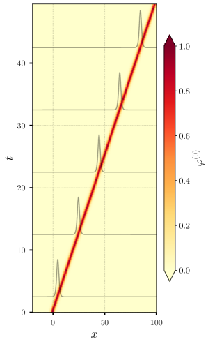
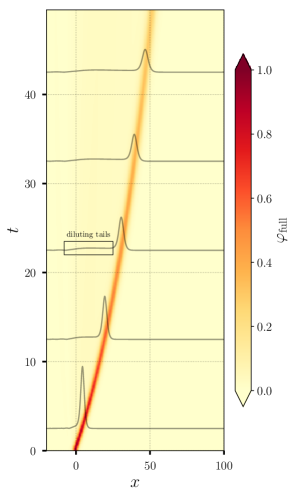
Figure 3: Left panel: Density plot and constant-time profiles (in black) of the analytic soliton solution in Eq. (72) for $v=2$. Right panel: Numerical solution of the KdVB equation for $\varepsilon=0.1$ using as an initial condition the same $v=2$ KdV soliton plotted in the left panel. The full solution can be approximated by a decelerating soliton with decreasing amplitude and increasing width, which can be captured by a renormalized solution $\varphi^{(0)}(\vec{\lambda}_{\text{R}})$. There is also a small step in the full solution (dubbed as “diluting tails” in the black rectangle), which makes the solution asymmetric. This tail is present in the residual $\varphi^{(1)}_{\perp}$ [see Eq. (60) and Fig. 6], and could be used to improve the renormalized solution.

To close this section, we summarize the algorithm one follows to build the renormalized solution at first order in $\varepsilon$:

1. Compute the differentials $\delta\varphi^{(0)A}/\delta\lambda^{i}$ for all parameters $\lambda^{i}$ whose flows you may attempt to renormalize. These differentials may be computed analytically, if an analytical solution is available, or numerically. Notice what powers of $(t-t_{0})$ appear in each basis function.

2. Solve the equations of motion in Eq. (27) and evaluate the naive perturbative solution, at many background points $\vec{\lambda}_{0}$ in the parameter space. Notice what powers of $(t-t_{0})$ appear in the naive perturbative solution $\varphi^{(1)A}$.

3. Consider a candidate set of parameters to try to fit. This will have to be determined individually for each problem, either by understanding the phenomenology of this problem, or by examining the features of $\varphi^{(1)A}$ and $\delta\varphi^{(0)A}/\delta\lambda^{i}$, and the different powers of $(t-t_{0})$ that appear in each. This will inform what order needs to be kept in expanding Eq. (45) using the BCH theorem [an example being Eq. (48)].

4. Build the cost function in Eq. (61) and extract $\psi$ for every simulation (each corresponding to a point $\vec{\lambda}_{0}$ in the parameter space). Examine $\varphi_{\perp}^{(1)A}$ to assess the quality of the fit of the perturbative solution as a combination of the basis function and the extracted flows. If the residual $\varphi^{(1)A}_{\perp}$ still exhibits secularly-growing features, go back to item 3 and consider more parameters, or expanding $\vec{V}$ to higher order in $(t-t_{0})$.

5. Once the fit has captured all the secularly-growing features, we can trust the extracted values of $\vec{\alpha}^{(1)}$ and $\vec{\beta}^{(1)}$, which can then be interpolated over the $\Lambda$ space. Solve the flow equations in Eq. (33) using $\vec{\lambda}_{\text{R}}(t_{0})=\vec{\lambda}_{0}+\varepsilon\vec{\alpha}^{(1)}(\vec{\lambda}_{0})$ as initial conditions for the renormalized parameters. The renormalized solution is $\varphi^{(0)}(\vec{\lambda}_{\text{R}})$, where $\vec{\lambda}_{\text{R}}$ solves the flow equations.

III Perturbing the KdV equation
and DRG extraction procedure

We now proceed to our main example, which is treating the Korteweg-de Vries-Burgers (KdVB) equation fully, using naive perturbation theory (which suffers from secular divergence), and with the numerical dynamical renormalization group approach. The one-dimensional KdVB equation [29] can be written as

$$\partial_{t}\varphi=-6\varphi\partial_{x}\varphi-\partial^{3}_{x}\varphi+\varepsilon\partial^{2}_{x}\varphi\,.$$ (69)

Dropping the third derivative term gives Burgers’ equation, while setting $\varepsilon=0$ gives the KdV equation. The KdV equation is integrable and admits soliton solutions. Throughout, we will treat the $\varepsilon$ term as a deformation of the KdV equation. This is a dissipation or diffusion term acting on a soliton, as seen in Fig. 3. It does not modify the principal part of the PDE, and thus does not affect the well-posedness of the problem.

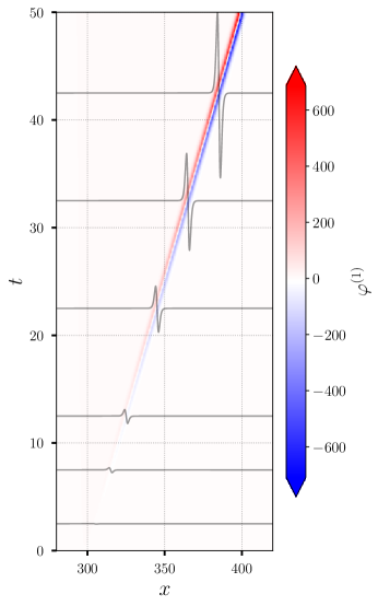
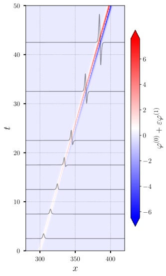
Figure 4: Left panel: Density plot and constant-time profiles (in black) with the solution of the perturbation equation in Eq. (75) for $v=2$. Right panel: Calculation of field at the first-order expansion in Eq. (25) for $\varepsilon=0.01$ following the standard prescription for perturbation theory. Secular divergences are visible in the amplitude at times $t\sim 1/\varepsilon$. In this figure, the range of the $x$-axis is different from Fig. 3 (this is simply a shift, allowed by translation invariance of the KdVB equation).

From now on, we use $\varphi_{\mathrm{full}}$ when referring to the full solution of the KdVB equation in Eq. (69). Using the naive perturbation ansatz, $\varphi=\varphi^{(0)}+\varepsilon\varphi^{(1)}$, we expand the solution up to the first order in $\varepsilon$. The background equation of motion is the well-known KdV equation,

$$\partial_{t}\varphi^{(0)}=-6\varphi^{(0)}\partial_{x}\varphi^{(0)}-\partial^{3}_{x}\varphi^{(0)}\,.$$ (70)

We are interested in background solutions which are a single soliton, of the form

$$\varphi^{(0)} =\frac{v}{2}\operatorname{sech}^{2}\left[\frac{\sqrt{v}}{2}(x-x_{0}-vt)\right]\,,$$ (71)

$$\varphi^{(0)} =\frac{v}{2}\operatorname{sech}^{2}\left[\frac{\sqrt{v}}{2}(x-x_{\mathrm{c}}(t))\right]\,.$$ (72)

This solution is parameterized by the two-dimensional parameter space of $\vec{\lambda}=(x_{0};v)$, where $x_{0}$ is the initial peak position, or $\vec{\lambda}=(x_{\text{c}};v)$, where the instantaneous peak position $x_{\mathrm{c}}$ is given by

$$x_{\mathrm{c}}(t)=x_{0}+\int_{t_{0}}^{t}v(t^{\prime})\,dt^{\prime}\,.$$ (73)

Using $x_{0}$ or $x_{\text{c}}$ as a coordinate choice in parameter space affects whether the background beta function vanishes or not. In the $x_{0}$ coordinate, $\vec{\beta}^{(0)}=0$. However, the time derivative of Eq. (73) shows that

$$\frac{dx_{\text{c}}}{dt}=v,\quad\vec{\beta}^{(0)}=v\frac{\partial}{\partial x_{\text{c}}}\,,$$ (74)

i.e., the parameter $v$ determines the zeroth-order beta function for the peak position $x_{\text{c}}$. This is analogous to how $\Omega_{0}$ generates the flow of $\phi_{\circ}(t)$ in Sec. II.1. Throughout we will use $x_{\text{c}}$, since at first order $\varepsilon$, we will anyway develop a non-zero beta function.

Since the KdVB equation is translation invariant, the dynamics can not depend on $x_{0}$, except for a trivial translation. Aside from the initial position, the one-soliton solution of Eq. (70) is determined by the velocity $v$, which simultaneously controls the amplitude ($v/2$), the width (proportional to $v^{-1/2}$), and the motion of the peak position (found by the integral in Eq. (73)).

We obtained numerical solutions for Eq. (69) and the perturbation equation [Eq. (75), below] using a pseudospectral method for space and the method of lines for time integration. We provide full details of the numerical method in Appendix A, the space and time scales involved, and the sources of error in the extraction of the beta functions (discussed in Sec. IV).

In Fig. 3, we plot the solutions for Eqs. (69) and (70), using a KdV soliton as an initial condition released at $x_{0}=0.0$ and $v=2.0$ in both of them. In the KdVB equation, the perturbative damping coefficient is $\varepsilon=0.1$. A key observation of the full solution is that, in principle, it is reasonable to build an approximate solution by modifying all the shape parameters of $\varphi^{(0)}$ – i.e., the amplitude, the width, the position, and velocity of the solitonic peaks – by time-dependent functions. This intuition provides us with a motivation to build such an approximate solution, which we will call $\varphi_{\mathrm{ren}}$ from now on, where the “bare” shape parameters are promoted to become functions of time. The main idea is that the initial conditions and the flow in time of the promoted parameters can be found by the renormalization procedure shown in Sec. II. Later in Sec. IV, we will also show that it is consistent to build $\varphi_{\mathrm{ren}}$ by renormalizing the bare $(x_{c};v)$ in the analytic KdV soliton of Eq. (72), rather than promoting the amplitude and width to independent parameters.

It is reasonable to expect that the renormalized solution does not contain all the information of the KdVB solution, such as the small step growing horizontally behind the decaying peak. These deviations, shown in a rectangle in the right panel of Fig. 3, become smaller as the damping parameter $\varepsilon$ reduces. We will show below that such deviations can be tabulated by computing the residual $\varphi^{(1)}_{\perp}$ as defined in Eq. (60). We defer to future work the problem of refining the renormalized solution with these small deviations.

We now proceed to (naive) first-order perturbation theory, where the equation of motion reads

$$\partial_{t}\varphi^{(1)}=\mathrm{KdV}^{(1)}\left[\varphi^{(1)}\right]+P\,.$$ (75)

Here the linear operator $\mathrm{KdV}^{(1)}$ acting on $\varphi^{(1)}$, and the source term $P$, are background-dependent, given by

$$\mathrm{KdV}^{(1)}\left[\varphi^{(1)}\right] \equiv\left[-6\varphi^{(0)}\partial_{x}-6\left(\partial_{x}\varphi^{(0)}\right)-\partial^{3}_{x}\right]\varphi^{(1)}\,,$$

$$P \equiv\partial^{2}_{x}\varphi^{(0)}\,.$$ (76)

It is important to keep in mind the explicit space/time dependence of $\varphi^{(0)}$ when solving this PDE for $\varphi^{(1)}$. In Fig. 4, we show the solution $\varphi^{(1)}$ of Eq. (75), and the reconstruction $\varphi^{(0)}+\varepsilon\varphi^{(1)}$ in naive perturbation theory, using $\varepsilon=0.01$. In this case, the perturbative solution has initial conditions $\varphi^{(1)}(t=0,x)=0$, and the background solution is taken to be a KdV soliton with $v=2.0$ started at $x_{0}=300.0$ at time $t=0$.

At early times, linear perturbation theory captures the effects of the damping term in slowing down the soliton. However, the perturbative solution eventually grows to an amplitude of $1/\varepsilon$, signaling the breakdown of naive perturbation theory. Similarly, the peak position differs by $\mathcal{O}(1)$ (in units of the soliton width) on a secular timescale $T_{\text{sec}}\sim\varepsilon^{-1/2}$. The first step to build an improved solution is to find which parameters need to be renormalized, by studying how the naive solution grows in time. We can compare the diverging features of $\varphi^{(1)}$ and the differentials $\delta\varphi^{(0)}/\delta\lambda^{i}$ to determine the vectors $\vec{\alpha}^{(1)}$ and $\vec{\beta}^{(1)}$ in order to renormalize the solution.

Space and time-translational invariance, as is the case of all symmetries, play an important role in determining the structure of the beta functions and, consequently, the renormalized parameters’ dependence. The solitonic solutions of Eqs. (69) and (70) are translational invariant since none of the terms contained in the equations of motion have an explicit spatial dependence. We expect, therefore, that the renormalized parameters do not depend on the peak position $x_{\text{c}}$. We also make the choice that the background kinematic relationship between $v$ and $x_{\text{c}}$ [Eq. (74)] continues to hold at higher orders in perturbation theory. Therefore we assume that the alpha and beta vectors take the form

$$\vec{\alpha}^{(1)}=\alpha^{v}(v)\frac{\partial}{\partial v},\quad\vec{\beta}^{(1)}=\beta^{v}(v)\frac{\partial}{\partial v}\,,$$ (77)

i.e. that we only renormalize the velocity. In principle, we can also add the shift $\alpha^{x_{\text{c}}}(v)\partial_{x_{\text{c}}}$, but this does not change our results drastically.

As in Sec. II, we construct the first-order solution in two ways: using naive perturbation theory, and with renormalized (flowing) parameters,

$$\varphi=\varphi^{(0)}+\varepsilon\varphi^{(1)}\quad\text{and}\quad\varphi=\varphi^{(0)}(\vec{\lambda}_{\text{R}}(t))+\varepsilon\varphi^{(1)}_{\perp}\,.$$ (78)

Here $\varphi^{(0)}$ is the one-soliton KdV solution in Eq. (72), $\varphi^{(1)}$ is the perturbative solution of Eq. (75), and $\varphi^{(1)}_{\perp}$ is the residual to be minimized. For short times, the renormalized parameters $\vec{\lambda}_{\text{R}}(t)\equiv\left(x^{\text{R}}_{\text{c}}(t);v_{\text{R}}(t)\right)$ can be computed by using the BCH formula as in Eq. (48),

$$\vec{\lambda}_{\text{R}} =\vec{\lambda}+\vec{V}\,,$$

$$\vec{V} =\varepsilon\left(\alpha^{v}\Delta t+\frac{\beta^{v}}{2}\Delta t^{2}\,;~{}\alpha^{v}+\beta^{v}\Delta t\right)\,,$$ (79)

where we made use of the background flow of Eq. (74). We find that the renormalized peak position $x_{\text{c}}(t)$ (derived from the composite flow in Eq. (45)) is consistent with our physical intuition of a point particle moving with constant acceleration. Here $\varepsilon\alpha^{v}$ gives an initial velocity shift, and $\varepsilon\beta^{v}$ gives an acceleration (the background moves at constant velocity). The form of the background flow and the dependence in Eqs. (74) and (77) have canceled all of the derivative corrections in Eqs. (51–54).

In analogy to the procedure in Eq. (60), we match the two expressions in Eq. (78) at first order in $\varepsilon$,

$$\varphi^{(1)}_{\perp}={} \varphi^{(1)}-d\varphi^{(0)}(\vec{V})\,,$$ (80)

where we must use (79), and the differential map,

$$d\varphi^{(0)}(\vec{V})\equiv{} \frac{\delta\varphi^{(0)}}{\delta x_{\mathrm{c}}}\left(\alpha^{v}\Delta t+\frac{\beta^{v}}{2}\Delta t^{2}\right)$$

$$+\frac{\delta\varphi^{(0)}}{\delta v}\left(\alpha^{v}+\beta^{v}\Delta t\right)\,.$$ (81)

The components of the differential map appearing are

$$\frac{\delta\varphi^{(0)}}{\delta v} =\frac{1}{2}\operatorname{sech}^{2}\xi\left[1+\xi\tanh\xi\right]\,,$$ (82)

$$\frac{\delta\varphi^{(0)}}{\delta x_{\mathrm{c}}} =\frac{v^{3/2}}{2}\operatorname{sech}^{2}\xi\tanh\xi\,,$$ (83)

where $\xi\equiv\sqrt{v}(x-x_{\mathrm{c}})/2$ and $x_{\mathrm{c}}=x_{0}+v\Delta t$. Now we have all the elements necessary extract $\alpha^{v}$ and $\beta^{v}$, for any value of $v$, by optimizing the cost functional in Eq. (63). In general, by dimensional analysis, the coefficients multiplying $\vec{\alpha}$ will always have a smaller power of $\Delta t$ than the corresponding coefficients multiplying $\vec{\beta}$. This means that at longer integration times, the optimization routine is more sensitive to $\vec{\beta}$ than it is to $\vec{\alpha}$.

IV Results

This section presents the results of the numerical DRG extraction procedure described in Sec. III for the KdVB problem. We use the extracted values of $\alpha^{v}$ and $\beta^{v}$ to build the renormalized solution $\varphi_{\mathrm{ren}}$. Our approach is not restricted to the original 2D parameterization of the one-soliton KdV solution, as written in Eqs. (72). We later consider the case of having additional independent shape parameters, such as the amplitude and the width of the soliton peak. We will also test if the renormalized solution is a good approximation by comparing it with the single-peaked solution of the KdVB equation.

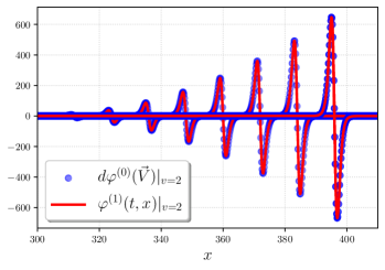
Figure 5: The perturbative solution $\varphi^{(1)}$ for $v=2$, and extracted $d\varphi^{(0)}(\vec{V})$, as functions of $(x,t)$, shown at different instants of time. The extracted values of $\alpha^{v}$ and $\beta^{v}$ make $d\varphi^{(0)}(\vec{V})$ a good fit to the perturbative solution.

IV.1 Original KdV parameterization

$v$	$\beta^{v}$	$\sigma_{\beta^{v}}$ (conv.)	$\sigma_{\beta^{v}}$ (RE)	$\alpha^{v}$	$\sigma_{\alpha^{v}}$ (conv.)	$\sigma_{\alpha^{v}}$ (RE)	$T_{\max}$
0.0625	$-1.010\times 10^{-3}$	$4.352\times 10^{-8}$	$3.050\times 10^{-5}$	$4.482\times 10^{-2}$	$4.287\times 10^{-5}$	$6.484\times 10^{-3}$	2400
0.125	$-4.184\times 10^{-3}$	$2.976\times 10^{-7}$	$2.170\times 10^{-6}$	$8.828\times 10^{-2}$	$1.809\times 10^{-4}$	$2.780\times 10^{-4}$	1500
0.25	$-1.667\times 10^{-2}$	$9.255\times 10^{-7}$	$2.064\times 10^{-5}$	$1.334\times 10^{-1}$	$7.459\times 10^{-4}$	$2.688\times 10^{-3}$	2000
0.5	$-6.672\times 10^{-2}$	$1.236\times 10^{-6}$	$6.887\times 10^{-6}$	$1.887\times 10^{-1}$	$2.980\times 10^{-4}$	$4.469\times 10^{-3}$	600
0.75	$-1.500\times 10^{-1}$	$9.266\times 10^{-7}$	$3.667\times 10^{-4}$	$2.311\times 10^{-1}$	$1.117\times 10^{-4}$	$5.953\times 10^{-3}$	300
1.0	$-2.667\times 10^{-1}$	$1.654\times 10^{-6}$	$2.250\times 10^{-5}$	$2.668\times 10^{-1}$	$1.991\times 10^{-4}$	$4.499\times 10^{-3}$	300
1.25	$-4.167\times 10^{-1}$	$2.587\times 10^{-6}$	$1.729\times 10^{-5}$	$2.982\times 10^{-1}$	$3.116\times 10^{-4}$	$3.629\times 10^{-3}$	300
1.5	$-6.000\times 10^{-1}$	$3.724\times 10^{-6}$	$1.406\times 10^{-5}$	$3.237\times 10^{-1}$	$4.490\times 10^{-4}$	$3.098\times 10^{-3}$	300
1.75	$-8.167\times 10^{-1}$	$5.064\times 10^{-6}$	$1.160\times 10^{-5}$	$3.530\times 10^{-1}$	$6.115\times 10^{-4}$	$2.666\times 10^{-3}$	300
2.0	$-1.067\times 10^{0\phantom{-}}$	$6.599\times 10^{-6}$	$9.526\times 10^{-6}$	$3.774\times 10^{-1}$	$7.989\times 10^{-4}$	$2.338\times 10^{-3}$	300

Table 1: Values of $\beta^{v}$ and $\alpha^{v}$ extracted at different values of $v$, as depicted in Fig. 8, and their corresponding uncertainties. Convergence errors are denoted $\sigma(\text{conv.})$ (see Appendix A), and Richardson extrapolation errors are denoted $\sigma(\text{RE})$, as depicted in Fig. 7. The values of $T_{\max}$ satisfy the condition for the soliton to translate much more than one width, $T_{\max}\gg v^{-3/2}$.

In the setup described in Sec. III, which considers a 2D parameter space $\vec{\lambda}\equiv(x_{\mathrm{c}},v)$, we made the ansatz to fit only the two components $\vec{\psi}=(\beta^{v},\alpha^{v})$. Consequently, the cost function $I$ to be minimized reduces to a 2-dimensional quadratic form

$$I={} \left[{\begin{array}[]{cc}\beta^{v}&\alpha^{v}\end{array}}\right]\left[\begin{array}[]{cc}\mathbb{M}^{(0)(0)}&\mathbb{M}^{(0)(1)}\\ \mathbb{M}^{(1)(0)}&\mathbb{M}^{(1)(1)}\end{array}\right]\left[\begin{array}[]{c}\beta^{v}\\ \alpha^{v}\end{array}\right]$$ (89)

$${}-2\left[{\begin{array}[]{cc}\beta^{v}&\alpha^{v}\end{array}}\right]\left[\begin{array}[]{c}\mathbb{V}^{(0)}\\ \mathbb{V}^{(1)}\end{array}\right]+\mathbb{D}\,.$$ (93)

Here $\mathbb{D}$ does not participate in the optimization procedure. We compute the matrix and vector coefficients of the vector of differentials $\vec{e}\equiv(e^{\beta};e^{\alpha})$, as detailed in Eq. (62),

$$\vec{e}=\bigg{(}\frac{\delta\varphi^{(0)}}{\delta x_{\mathrm{c}}}\frac{\Delta t^{2}}{2}+\frac{\delta\varphi^{(0)}}{\delta v}\Delta t;~{}\frac{\delta\varphi^{(0)}}{\delta x_{\mathrm{c}}}\Delta t+\frac{\delta\varphi^{(0)}}{\delta v}\bigg{)}\,,$$ (94)

yielding the coefficients in Eq. (89),

$$\mathbb{M}^{(\mu)(\nu)} =\int_{L}dx\int_{t=t_{0}}^{t=T_{\max}}dt\>e^{(\mu)}e^{(\nu)}\,,$$ (95)

$$\mathbb{V}^{(\mu)} =\int_{L}dx\int_{t=t_{0}}^{t=T_{\max}}dt\>\varphi^{(1)}e^{(\mu)}\,,$$ (96)

where $L$ is the length of the simulation box, and $T_{\max}$ is the total evolution time of the perturbative solution. We find the vector of optimum values containing $\beta^{v}$ and $\alpha^{v}$ by performing the same matrix inversion introduced in Eq. (68); since the matrix is just $2\times 2$, this is

$$\begin{bmatrix}\beta^{v}\\ \alpha^{v}\end{bmatrix}=\frac{1}{\det\mathbb{M}}\begin{bmatrix}\mathbb{M}^{(1)(1)}&-\mathbb{M}^{(0)(1)}\\ -\mathbb{M}^{(1)(0)}&\mathbb{M}^{(0)(0)}\end{bmatrix}\mathbb{V}\,.$$ (97)

Once we have the extracted values of $\alpha^{v}$ and $\beta^{v}$, it is crucial to test the quality of the linear decomposition of $\varphi^{(1)}$ in terms of the basis functions in Eqs. (82) and (83). From the definition of $\varphi^{(1)}_{\perp}$ in Eq. (80), we compare $\varphi^{(1)}$ and $d\varphi^{(0)}(\vec{V})$ in Fig. 5, showing a good fit of the perturbative solution as a linear decomposition in basis functions for $v=2.0$. The quality of the fit is due to both the correct choice of basis functions and the correct values of $\alpha^{v}$ and $\beta^{v}$. The quality of the fit also shows if we have considered an appropriate time-dependence of the infinitesimal shift $\vec{V}$. We define the relative difference

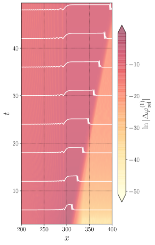
Figure 6: Color: The relative difference $\Delta\varphi^{(1)}_{\mathrm{rel}}$ for $v=2$ remains small for the duration of the simulation. White curves: The residual $|\varphi^{(1)}_{\perp}|$ (not scaled by the max) at different times, growing in spatial extent. This feature coincides with the bump due to the “diluting tails” in the right panel of Fig. 3.

$$\Delta\varphi^{(1)}_{\mathrm{rel}}(t,x)\equiv\frac{\varphi^{(1)}_{\perp}(t,x)}{\max_{x^{\prime}}\varphi^{(1)}(t,x^{\prime})},$$ (98)

to corroborate the goodness of the fit even at late times. In Fig. 6, we observe that the relative difference is never greater than $10^{-5}$ for $T_{\max}=50$. Interestingly, the residual $\varphi^{(1)}_{\perp}$ (plotted in white) has the same shape as the “diluting tails” shown in the right panel of Fig. 3, suggesting that it is possible to also recover the “instantaneous” perturbative features (those not captured by renormalization) of the full solution with a refinement of this method.

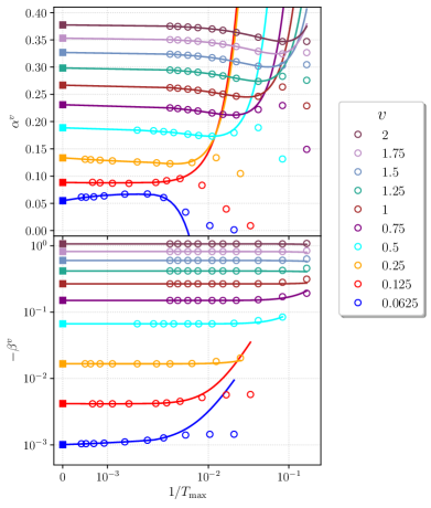
Figure 7: Quadratic RE in the limit $1/T_{\max}\to 0$. The extrapolated values (filled squares) correspond to the values of $\alpha^{v}$ and $\beta^{v}$ in Table 1. The extrapolating polynomial (solid line) is a quadratic in powers of $T_{\max}^{-1}$, hence the unphysical blowup to the right.

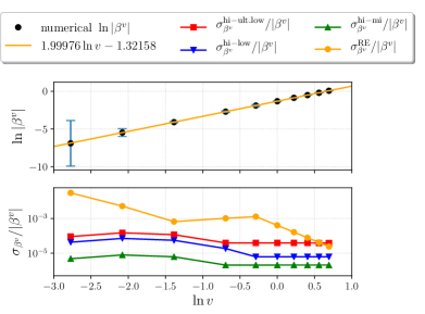
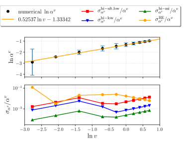
Figure 8: Power law fits to the Richardson-extrapolated values of $\beta^{v}$ and $\alpha^{v}$, as a function of $v$. Upper panels: Best fit for the alpha and beta functions (in orange) with enlarged error bars (in blue), estimated as due to RE. Error bars were enlarged by a factor of $10^{2}$ for $\ln|\beta^{v}|$, and by a factor of $10$ for $\ln\alpha^{v}$. Lower panels: Magnitude of the fractional errors from different sources. $\sigma^{\text{RE}}$ is the difference between the values of $\alpha^{v}$ and $\beta^{v}$ extracted by RE, and the values at finite $T_{\max}$ (the last column of Table 1). Convergence errors are obtained by comparing the extracted quantities at four different resolutions, named high (hi), mid (mi), low (low), and ultra-low (ult.low). The error bars in the upper panels are $\sigma^{\text{RE}}$, which are larger than convergence errors.

The upper limit in the integration time ($T_{\max}$ in Eqs. (95) and (96)) plays a significant role in evaluating the stability of the extracted alpha and beta functions. If $T_{\max}$ is too short, the specific choice of initial conditions becomes a dominant feature of the solution. Therefore, it is prudent to evaluate the perturbative solution $\varphi^{(1)}$ for a sufficiently long time. A minimal consistency condition for the evolution of the system is that, knowing the that the width of the soliton is roughly given by $v^{-1/2}$, $T_{\max}\gg v^{-3/2}$ ensures that the perturbative solution has displaced a distance much larger than a single soliton width. We perform the integration for a variety of values of $T_{\max}$, and then use (quadratic) Richardson extrapolation (RE) [35, 36] in powers of $T_{\max}^{-1}$ to find the generators $\beta^{v}$ and $\alpha^{v}$ in the limit $T_{\max}\to\infty$, and estimate their corresponding errors, for different values of $v$. In Fig. 7, we show the way the RE works, finding the values of $\alpha^{v}$ and $\beta^{v}$ (in colored squares) reported in Table 1. From this figure, we notice how the extracted values of $\alpha^{v}$ and $\beta^{v}$ smoothly converge to the extrapolated values as $T_{\max}\to\infty$. Moreover, it is clear that the extracted values of $\beta^{v}$ and $\alpha^{v}$ (empty circles) do not show large variations as $T_{\max}$ grows. We observe that all of the values of $\beta^{v}$ are negative, in agreement with the notion of a decelerating peak, as shown by the non-linear solution plotted the in the right panel of Fig. 3. We estimate the errors arising from RE (denoted $\sigma\text{(RE)}$) from the difference between the extrapolated values and the extracted values from the largest $t=T_{\max}$ of each simulation.

Table 1 shows the values of $\alpha^{v}$ and $\beta^{v}$ extrapolated from each of the simulations, and their corresponding errors. The main sources of error are (a) the numerical calculation of the perturbative solution $\varphi^{(1)}$, and (b) the fact that simulations are evaluated at finite (but large) values of $T_{\max}$. Even when these sources of error can be combined, we chose to treat them independently. The numerical convergence error is further discussed in Appendix A.

For a general application of the numerical DRG, one would have to rely on interpolation of $\vec{\alpha}^{(1)},\vec{\beta}^{(1)}$ over the $\vec{\lambda}$ parameter space, in order to numerically solve the $\beta$ function equations. For our particular problem of the KdVB equation, we can make an argument that $\alpha^{v}(v)$ and $\beta^{v}(v)$ will be pure power laws in $v$ (this analytical argument only came after our numerical explorations). The background ($\varepsilon=0$) KdV equation has a scaling symmetry, such that if $\varphi(t,x)$ is a solution, then so is $\gamma^{2}\varphi(\gamma^{3}t,\gamma x)$. This corresponds to a simultaneous change of length and time units, under which velocity should change to be $\gamma^{-2}v$; and dimensional analysis shows that $\varepsilon$ should change to be $\gamma^{-1}\varepsilon$. We expect the renormalized solution will inherit the background’s symmetry. We allow some undetermined transformations $\alpha^{v}\to\gamma^{c}\alpha^{v}$ and $\beta^{v}\to\gamma^{d}\beta^{v}$. Applying the scaling transformation to the infinitesimal flow, we have

$$v \to v+\varepsilon(\alpha^{v}+\beta^{v}\Delta t)\,,$$ (99)

$$\gamma^{-2}v \to\gamma^{-2}v+\gamma^{-1}\varepsilon(\gamma^{c}\alpha^{v}+\gamma^{d}\beta^{v}\gamma^{3}\Delta t)\,.$$ (100)

We find the powers $c$ and $d$ in order to make this homogeneous in $\gamma$, namely, $c=-1$ and $d=-4$. This is satisfied with $\alpha^{v}\propto v^{1/2}$ and $\beta^{v}\propto v^{2}$. As we were completing this manuscript, we learned of Ref. [37], whose results also imply a power-law for $\beta^{v}$. Therefore, instead of using interpolating functions, we fit power laws for $\alpha^{v}$ and $\beta^{v}$.

Given the extrapolated values in Table 1, we use the ansatz

$$\ln|\beta^{v}|=m\ln v+b\,,$$ (101)

and similarly for $\alpha^{v}$. The best fit power law is plotted in the upper panels of Fig. 8. The fractional error bars are plotted in the bottom panels, which are too small to see without magnification in the top panels; we omit error bars in later plots. The quality of the fit needs to be as good as possible, since errors in the fit will incur secular errors in the renormalized solution. Later, in Sec. IV.3, we will compare the renormalized solution against the full solution of the KdVB equation.

We used the standard non-linear fit routine curve_fit in scipy [38], with weights coming from the estimated RE errors (the convergence errors are much smaller, as seen in the lower panels of Fig. 8; see Appendix A for full details on convergence testing). The curve_fit routine returns the optimal fits, in Table 2, and covariance matrix estimates on the two parameters $(m,b)$ for each of the two fits,

$$\Sigma^{2}_{\beta^{v}} =\begin{bmatrix}8.7\times 10^{-9}&-5.5\times 10^{-9}\\ -5.5\times 10^{-9}&3.6\times 10^{-9}\end{bmatrix},$$ (102)

$$\Sigma^{2}_{\alpha^{v}} =\begin{bmatrix}4.8\times 10^{-6}&5.1\times 10^{-6}\\ 5.1\times 10^{-6}&1.3\times 10^{-5}\end{bmatrix}\,.$$ (103)

These fits agree (very well for $\beta^{v}$, less so for $\alpha^{v}$) with the scaling argument for the power laws $\beta^{v}\propto v^{2}$ and $\alpha^{v}\propto v^{1/2}$. The quality of both fits improves (more substantially for $\alpha^{v}$) if we omit the point with $v=0.0625$.

	$m$	$b$
$\beta^{v}$	$1.99976\pm 9.3\times 10^{-5}$	$-1.32158\pm 6.0\times 10^{-5}$
$\alpha^{v}$	$0.52537\pm 2.2\times 10^{-3}$	$-1.33342\pm 3.6\times 10^{-3}$

Table 2: Linear regression coefficients and errors for $\ln|\beta^{v}|$ and $\ln\alpha^{v}$ as functions of $\ln v$.

With these $\alpha$ and $\beta$ functions in hand, we can now construct the renormalized solution $\varphi_{\text{ren}}=\varphi^{(0)}(\vec{\lambda}_{\text{R}})$ as a semi-analytic expression of the form

$$\varphi^{(0)}(\vec{\lambda}_{\text{R}})=\frac{v_{\text{R}}(t)}{2}\operatorname{sech}^{2}\left[\frac{\sqrt{v_{\text{R}}(t)}}{2}(x-x^{\text{R}}_{\mathrm{c}}(t))\right]\,.$$ (104)

This approximate solution is simply constructed by replacing $v\rightarrow v_{\text{R}}(t),~{}x_{c}(t)\to x_{c}^{\text{R}}(t)$ in the background solution of Eq. (72), where these components of $\vec{\lambda}_{\text{R}}$ satisfy the flow equations

$$\frac{dv_{\text{R}}}{dt} =0+\varepsilon\beta^{v}(v_{\text{R}})=-\varepsilon\,e^{b}\,v_{\text{R}}^{m}\,,$$ (105)

$$\frac{dx_{c}^{\text{R}}}{dt} =v_{\text{R}}+\varepsilon\beta^{x_{c}}=v_{\text{R}}\,,$$ (106)

subject to the initial condition $v_{\text{R}}(t_{0})=v_{0}+\varepsilon\alpha^{v}(v_{0})$ reparameterized by $\alpha^{v}$, whereas $x_{c}^{\text{R}}(t_{0})$ is not shifted, according to the argument above Eq. (77). The values in Table 2 suggest that the analytical $\beta$ function is

$$\beta^{v}=-\frac{4}{15}v^{2}\,.$$ (107)

As we were completing this manuscript, we learned of an analytical calculation in [37] which implies this same $\beta$ function. If one takes a time derivative of their Eq. (53), and performs some algebra, one can recover our Eq. (107).

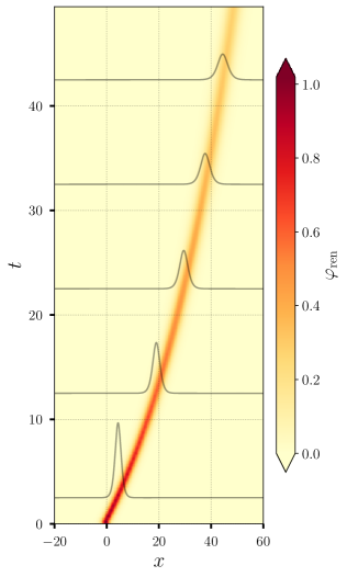
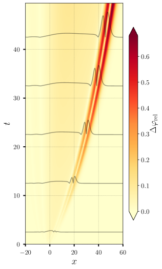
Figure 9: Left panel: Renormalized solution in Eqs. (104) for $v=2$ and $\varepsilon=0.1$ built from the solution of the renormalized flow of Eqs. (105–106). Here the damping effects can be clearly noticed as the peak decelerates, its amplitude attenuates, and it becomes broader. Right panel: Fractional difference between the renormalized and full solutions. The small difference between the position of the peaks is visible in the separation of the two red density profiles. The peaks of the renormalized and full solutions have very similar amplitudes. At $t=50$ (much longer than $\varepsilon^{-1/2}$), the distance between the peaks is roughly half a peak width.

In Fig. 9, we show the renormalized solution for $\varepsilon=0.1$, and compare it with the one-soliton solution of the KdVB equation. From the left panel of this figure, it is clear that the amplitude of the renormalized solution does not increase as the naive perturbative solution plotted in the right panel of Fig. 4. Moreover, this evolving solution is not substantially different from the KdVB solution depicted in the right panel of Fig. 3, except for the absence of the small step dubbed as “diluting tails” in the evolution of $\varphi_{\text{full}}$. In the right panel, we depict the difference between the renormalized expression and the full solution by introducing a fractional difference variable, $\Delta\varphi_{\mathrm{rel}}$, defined as

$$\Delta\varphi_{\mathrm{rel}}(t,x)\equiv\frac{\varphi_{\mathrm{full}}(t,x)-\varphi_{\mathrm{ren}}(t,x)}{\max_{x^{\prime}}\varphi_{\mathrm{full}}(t,x^{\prime})},$$ (108)

where the expression in the denominator corresponds to the decreasing amplitude of the peak at each instant of time. The main differences between the full and the renormalized solutions are the presence of diluting tails in the solution (a horizontally-growing “bump” to the left of the two peaks, which was also visible in the black rectangle of the right panel of Fig. 3), and the secular position error between the peaks. It is interesting to note that the magnitude of the “diluting tails” coincides with the residual $\varphi^{(1)}_{\perp}$ multiplied by $\varepsilon$, as plotted in Fig. 6.

The initial shift $v\rightarrow v+\varepsilon\alpha^{v}$ changes the initial soliton’s amplitude, velocity, and width by a small amount compared to the original shape parameters. At time $t=0$, this small change only amounts to around 3% of the amplitude. However, if we had omitted the $\alpha^{v}$ reparameterization, the maximum fractional error $\Delta\varphi_{\mathrm{rel}}$ secularly grows, increasing by $10\%$ by $t=50$, due to starting with the wrong initial velocity.

The main question about the renormalized solution is whether it captures secular effects of the true solution, which has several secular timescales. For quantities whose background flow vanishes, the estimate $T_{\text{sec}}\sim(\varepsilon\beta^{(1)})^{-1}$ of Sec. II.2 is still valid. These quantities include the velocity, and derived features such as the width and amplitude. Investigating our solution, we find that the velocity error is bounded, even on much longer times, $t\gg(\varepsilon\beta^{(1)})^{-1}$. The amplitude and width follow the same behavior. These differences will be further detailed in Sec. IV.3.

However, the peak position is sensitive to an even shorter timescale, due to the “deceleration” of the peak, and this leads to the dominant error. The background flow Eq. (74) generates the acceleration-like term $\varepsilon\Delta t^{2}$ in the infinitesimal generator $\vec{V}$ in Eq. (79). This leads to the shorter secular time scale

$$T_{\text{sec}}\sim\frac{1}{\sqrt{\varepsilon\beta^{v}}}\,.$$ (109)

Notice that the difference between the renormalized peak position and the full solution is only half the peak’s width at $t=50$. This time $t=50$ is vastly longer than the secular time $(\varepsilon\beta^{v})^{-1/2}\approx 1.9$ for $v=2$ and $\varepsilon=0.1$. Naive perturbation theory had already failed by this time $T_{\text{sec}}$. Thus, the renormalized solution presented in Eq. (104) represents $\varphi_{\text{full}}$ far better than the naive perturbative expression $\varphi^{(0)}+\varepsilon\varphi^{(1)}$ in Eq. (25).

In what remains of this section, we will introduce the amplitude, width, and peak position as additional independent parameters of the system. We evaluate their corresponding alpha and beta functions using (a) our minimization scheme, and (b) by direct evaluation of the KdVB solution (in Sec. IV.3). We will verify that the renormalized solution can be written using only two flowing parameters, $(x_{c}(t),v)\rightarrow(x^{\text{R}}_{c}(t),v_{\text{R}}(t))$, similar to the background KdV soliton. This also allows us to perform a more detailed comparison of the features between the renormalized and full solutions. The reader can safely skip these subsections to learn about different applications of this technique in Sec. V.

IV.2 Alternative parameterizations:
the multiparameter case

One potential unknown in the numerical DRG procedure is whether the parameterization for the renormalized solution is sufficiently general. It can happen that the background problem has one dimensionality, but upon being perturbed, the dimensionality increases [21]. In this subsection, we check if this happens in our KdV example by proposing a higher-dimensional parameterization for the background KdV soliton. This allows us to confirm that our previous two-dimensional parameterization was actually sufficient, by testing the consistency between different parameters’ flows. We parametrize the zeroth-order solution by labelling the shape parameters as

$$\varphi^{(0)}=\mathcal{A}\operatorname{sech}^{2}\left[\mathcal{M}\left(x-x_{\mathrm{c}}\right)\right]\,,$$ (110)

where we can identify the amplitude $\mathcal{A}=v/2$ and inverse width $\mathcal{M}=\sqrt{v}/2$, in terms of the original parameters of the KdV solution. If these background relationships are maintained upon renormalization, then we would have the relationships

$$\alpha^{\mathcal{A}} =\frac{\alpha^{v}}{2}\,, \alpha^{\mathcal{M}} =\frac{\alpha^{v}}{4\sqrt{v}}\,,$$ (111)

$$\beta^{\mathcal{A}} =\frac{\beta^{v}}{2}\,, \beta^{\mathcal{M}} =\frac{\beta^{v}}{4\sqrt{v}}\,.$$ (112)

If these relationships are maintained, then the flows are tangent to a 2-dimensional solution manifold described by $(x_{\mathrm{c}};v)$, within the ambient 4-dimensional space $\vec{\lambda}=(\mathcal{A};\mathcal{M};x_{c};v)$. This is similar to the example in Sec. II.1, where we saw that the $R_{\text{R}}$ and $\Omega_{\text{R}}$ components of the $\beta$ function in Eq. (20) are not independent – they are related by preserving the form of Kepler’s law.

To check the dimensionality, we calculate the first-order beta functions for $\mathcal{A}$ and $\mathcal{M}$ following the same renormalization-based scheme suggested in Sec. II, as well as in previous instances of the current subsection. To do so, first we pose the $\vec{\alpha},\vec{\beta}$ ansatz

$$\vec{\beta}^{(0)}=v\frac{\partial}{\partial x_{\text{c}}}\,,$$ (113)

$$\vec{\alpha}^{(1)}=\alpha^{\mathcal{A}}(v)\frac{\partial}{\partial\mathcal{A}}+\alpha^{\mathcal{M}}(v)\frac{\partial}{\partial\mathcal{M}}+\alpha^{v}(v)\frac{\partial}{\partial v}\,,$$ (114)

$$\vec{\beta}^{(1)}=\beta^{\mathcal{A}}(v)\frac{\partial}{\partial\mathcal{A}}+\beta^{\mathcal{M}}(v)\frac{\partial}{\partial\mathcal{M}}+\beta^{v}(v)\frac{\partial}{\partial v}\,,$$ (115)

where the addition of a shift in the initial peak position $\alpha^{x_{\text{c}}}(v)\partial_{x_{\text{c}}}$ does not alter our results significantly. This gives the flow equations

$$\frac{d\mathcal{A}_{\text{R}}}{dt} =0+\varepsilon\beta^{\mathcal{A}}(v_{\text{R}})\,, \frac{d\mathcal{M}_{\text{R}}}{dt} =0+\varepsilon\beta^{\mathcal{M}}(v_{\text{R}})\,,$$ (116)

$$\frac{dv_{\text{R}}}{dt} =0+\varepsilon\beta^{v}(v_{\text{R}})\,, \frac{dx^{\text{R}}_{\text{c}}}{dt} =v_{\text{R}}+\varepsilon\beta^{x_{\text{c}}}=v_{\text{R}}\,,$$ (117)

that is, $(\mathcal{A};\mathcal{M};v)$ have vanishing background flows, and the flow of $x_{c}$ maintains its kinematic meaning.

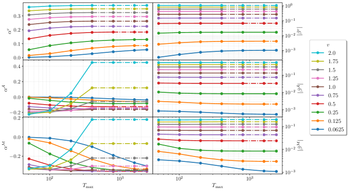
Figure 10: All the values of $\alpha$ and $\beta$ for different values of $T_{\max}$. Dashed lines represent the intervals of $T_{\max}$ where the values of $\alpha$ or $\beta$ have not been computed. All the beta functions have converged to a fixed value before the dashed lines, but $\alpha^{\mathcal{A}}$ and $\alpha^{\mathcal{M}}$ have not converged to stable values at large $T_{\max}$. This indicates that we have not found their correct time dependence at the infinitesimal level.

Now we compute the first-order deformation flow $\vec{V}$ using the BCH theorem in Eq. (II.2.1), which in the $(\mathcal{A};\mathcal{M};x_{\text{c}};v)$ coordinates is given by

$$\vec{\lambda}_{\text{R}}={} \vec{\lambda}+\vec{V}\,,$$

$$\vec{V}={} \varepsilon\big{(}\alpha^{\mathcal{A}}+\beta^{\mathcal{A}}\Delta t;~{}\alpha^{\mathcal{M}}+\beta^{\mathcal{M}}\Delta t;$$

$$\quad\alpha^{v}\Delta t+\frac{\beta^{v}}{2}\Delta t^{2};~{}\alpha^{v}+\beta^{v}\Delta t\big{)}\,.$$ (118)

Next we compute the differentials by taking partial derivatives of Eq. (110), which are given by

$$\frac{\delta\varphi^{(0)}}{\delta\mathcal{A}}=\operatorname{sech}^{2}\xi,$$ (119)

$$\frac{\delta\varphi^{(0)}}{\delta\mathcal{M}}=-4\mathcal{M}\xi\operatorname{sech}^{2}\xi\tanh\xi,$$ (120)

$$\frac{\delta\varphi^{(0)}}{\delta x_{\mathrm{c}}}=4\mathcal{M}^{3}\operatorname{sech}^{2}\xi\tanh\xi,$$ (121)

$$\frac{\delta\varphi^{(0)}}{\delta v}=0\,.$$ (122)

Here $\xi\equiv\sqrt{v}(x-x_{\mathrm{c}})/2$, and $x_{\mathrm{c}}=x_{0}+v\Delta t$ follows from the background flow definitions in Eqs. (74) and (113). It is worth mentioning that the new parameterization splits the original dependence in $v$, seen in Eq. (72), between $\mathcal{A}$ and $\mathcal{M}$. The only $v$ dependence is in the implicit background flow of the peak position $x_{c}$ – there is no explicit $v$ dependence. This causes the differential $\delta\varphi^{(0)}/\delta v$ to vanish in Eq. (122).

To extract $\vec{\alpha}^{(1)}$ and $\vec{\beta}^{(1)}$, we reuse the previous numerically-computed naive first-order solutions of Eq. (75), with the same velocities as before. We calculate $\varphi^{(1)}_{\perp}$ as the residual after fitting the perturbative solution $\varphi^{(1)}$ as a linear combination of basis functions, in the same way detailed in Sec. II, and build a new cost function $I$ for this case,

$$I={} \int_{L}dx\int_{t_{0}}^{T_{\max}}dt\>\bigg{\{}\varphi^{(1)}-\frac{\delta\varphi^{(0)}}{\delta x_{\mathrm{c}}}\left(\alpha^{v}\Delta t+\frac{\beta^{v}}{2}\Delta t^{2}\right)$$

$$-\left[\frac{\delta\varphi^{(0)}}{\delta\lambda^{j}}\left(\alpha^{j}+\beta^{j}\Delta t\right)\right]\bigg{\}}^{2}\,.$$ (123)

Here $j$ sums over the parameters in the subspace $\vec{\lambda}=(\mathcal{A};\mathcal{M};v)$. As before we minimize $I$, looking for the critical point $\delta I/\delta\vec{\psi}=0$, giving the six-dimensional vector $\vec{\psi}=(\vec{\alpha}^{(1)},\vec{\beta}^{(1)})$.

Examining the extracted values $\vec{\alpha}^{(1)}$ and $\vec{\beta}^{(1)}$, as functions of $T_{\max}$, is crucial to verify if the time dependence and perturbative order proposed in Eq. (IV.2) is sufficient to capture the parameter flows. In Fig. 10, we show that all the beta functions smoothly converge to fixed values when $T_{\max}$ is sufficiently long, which provides clear evidence of finding the correct time dependence in $\vec{V}$. Interestingly, there are no significant differences between (a) the values of $\alpha^{v}$ and $\beta^{v}$ extracted from the minimization procedure in the 2D parameter case (in Sec. IV.1), and (b) the ($\alpha^{v},\beta^{v}$) values extracted using the 4D parameterization in this section. The dashed lines represent values of $T_{\max}$ longer than the simulation time, where the alpha and beta functions have not been extracted.

In all of the cases we plotted, the beta functions have converged to a stable value within the simulation time. Meanwhile, even though $\alpha^{v}$ is stable with $T_{\max}$, the same cannot be said about all of the alpha functions: $\alpha^{\mathcal{A}}$ and $\alpha^{\mathcal{M}}$ have not converged to stable values by a time $T_{\max}\approx 10^{3}$. This may be due to the minimization of $I$ being more sensitive to $\beta^{i}$ than to $\alpha^{i}$, since, by dimensional analysis, there is one more factor of $\Delta t$ in front of $\beta^{i}$. It is possible that this parameterization is insufficient, or that going to higher order in $\varepsilon$ or $\Delta t$ would improve the convergence of these $\alpha$’s.

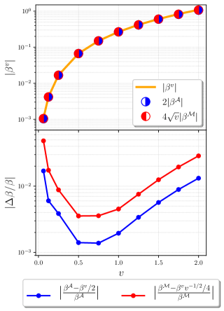
Figure 11: Testing tangent flows in parameter space as a function of $v$. In the upper panel, we observe that $\beta^{v}$, $2\beta^{\mathcal{A}}$, and $4\sqrt{v}\beta^{\mathcal{M}}$ are consistent with the relations in Eq. (112). In the lower panel, we plot the relative deviations in the reconstructed $\beta^{\mathcal{A}}$ and $\beta^{\mathcal{M}}$ against the appropriate function of $\beta^{v}$ if the flow is tangent; the deviations are of the order of 1%.

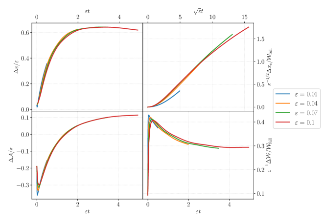
Figure 12: Comparing the shape parameters of the KdVB solution (for four $\varepsilon$ values) versus the parameters of the renormalized solution $\varphi_{\text{ren}}$, as functions of time. The errors in peak velocity $\Delta v$ and amplitude $\Delta\mathcal{A}$ are bounded in time, and proportional to $\varepsilon$, even for times significantly larger than $1/\sqrt{\varepsilon}$. The error in peak position $\Delta x_{c}$ (in units of width) is linear in time and linear in $\varepsilon$ at late times, due to the bounded velocity error. $\Delta\mathcal{W}/\mathcal{W}_{\text{full}}$ is linear in $\varepsilon$, bounded, and approaches a constant for $t\gg 1/\sqrt{\varepsilon}$.

Since $\alpha^{\mathcal{A}}$ and $\alpha^{\mathcal{M}}$ have not converged, we can not check the consistency conditions in Eq. (111). But, we can check the $\beta$ function tangency conditions in Eq. (112). In the upper panel of Fig. 11, we show $|\beta^{v}|$ and what should be two equivalent expressions, if tangency is satisfied: $2|\beta^{\mathcal{A}}|$, and $4\sqrt{v}|\beta^{\mathcal{M}}|$. In the lower panel, we plot the fractional errors $|(\beta^{v}/2-\beta^{\mathcal{A}})/\beta^{\mathcal{A}}|$ and $|(v^{-1/2}\beta^{v}/4-\beta^{\mathcal{M}})/\beta^{\mathcal{M}}|$, finding that the deviations from a tangent flow are very small. The errors in the tangency conditions for $v<0.5$ can be reduced by increasing the resolution (though this is computationally expensive, since we must increase $T_{\max}$ as $v$ becomes smaller).

The conclusion seems to be that the $\beta$ functions for the flow are consistent with being tangent to the two-dimensional submanifold. Meanwhile, the $\alpha$ functions setting the initial conditions can not be tested for consistency, since only $\alpha^{v}$ has converged. This type of test would be prudent when applying the numerical DRG, unless one knows a priori the functional form of the renormalized solutions.

IV.3 Comparing DRG $\alpha$ and $\beta$ functions
against the full KdVB solution

In this subsection, we extract the amplitude, width, position, and velocity of the peak from the single-peaked solution of the full KdVB equation of Eq. (69), as well as their evolution in time. The study of the full solution enables us to explore the $\varepsilon$-dependence of DRG, and the accuracy of the $\alpha$ and $\beta$ functions extracted using the procedure described in Section II. To do so, we first need to determine the peak position, amplitude, and width at each time of both $\varphi_{\text{ren}}$ and $\varphi_{\mathrm{full}}$. For the renormalized solution, we numerically integrate the flow Eqs. (105) and (106) using our numerical fits. This immediately gives $v_{\text{R}}(t)$ and $x^{\text{R}}_{c}(t)$. We get the renormalized amplitude $\mathcal{A}_{\text{R}}=v_{\text{R}}/2$ from the background relationship. For the width, we use the full width at half max (FWHM): the difference in $x$ values where the value of $\varphi(x)$ is half of its peak value. From the form of the soliton solution, this is given by

$$\mathcal{W}_{\text{R}}=\frac{4\cosh^{-1}\sqrt{2}}{\sqrt{v_{\text{R}}(t)}}\approx\frac{3.525}{\sqrt{v_{\text{R}}(t)}}\,.$$ (124)

We caution that although the symbol $\mathcal{M}$ used throughout Sec. IV.2 has units of inverse width, it is not exactly the reciprocal of the FWHM $\mathcal{W}$ that we use in this section – they differ by a multiplicative constant.

To find the same parameters from the full solution, we use Fourier interpolation [39] to evaluate $\varphi_{\text{full}}$ at points not tabulated in the collocation grid. We use Newton’s method to root-solve for the peak location $x^{\text{full}}_{c}(t)$, determined by

$$\frac{\partial\varphi_{\text{full}}}{\partial x}\bigg{|}_{x=x^{\text{full}}_{\mathrm{c}}}=0\,.$$ (125)

We can calculate the instantaneous velocity $v^{\text{full}}$ of the peak for $\varphi_{\mathrm{full}}$ by calculating the numerical time derivative of the peak position. In our implementation, we used a fourth-order accurate finite difference (we only evaluate at interior times so that we only need to implement the central finite difference). Once we find the peak position, we obtain the amplitude of the peak at each time,

$$\mathcal{A}_{\mathrm{full}}(t)=\varphi_{\text{full}}(t,x^{\text{full}}_{c}(t))\,,$$ (126)

again using spectral interpolation.

Calculating the FWHM of the peak $\mathcal{W}_{\text{full}}$ from $\varphi_{\mathrm{full}}$ requires finding the set of two points $x_{1/2(>)}$ and $x_{1/2(<)}$, to the right and left of the peak, satisfying

$$\varphi_{\mathrm{full}}(t,x_{1/2(\lessgtr)})=\frac{\mathcal{A}_{\mathrm{full}}(t)}{2}$$ (127)

at each instant of time. We again use Fourier interpolation and Newton root-polishing. Then the FWHM at a given instant of time is $\mathcal{W}_{\mathrm{full}}=x_{1/2(>)}-x_{1/2(<)}$. Notice that the peak is asymmetric due to the presence of the “diluting tails” in the full solution.

Once we have calculated the values of the shape parameters from both the full and the renormalized solutions, we compare our results by defining the difference

$$\Delta\mathcal{W}\equiv\mathcal{W}_{\mathrm{full}}-\mathcal{W}_{\text{R}}\,,$$ (128)

and similarly for the amplitude $\mathcal{A}$, the peak velocity $v$, and the peak position $x_{c}$. In Fig. 12, we show the evolution of the errors of all of these quantities, at four different values of the perturbation parameter $\varepsilon$, for simulations with $v=2$. We see that $\Delta v$, $\Delta\mathcal{A}$, and the relative error $\Delta\mathcal{W}/\mathcal{W}_{\text{full}}$ are bounded in time. We scale these three quantities by $\varepsilon^{-1}$, showing that each is proportional to $\varepsilon$. Similarly we used $\varepsilon t$ as the time axis for these three panels, showing that our solutions are valid at secularly-large times, $t\gg\varepsilon^{-1}\gg\varepsilon^{-1/2}$. For the values of $\varepsilon$ reported in the figure, we observe that the difference $\Delta\mathcal{W}$ is never larger than 4.5% of the FWHM $\mathcal{W}_{\text{full}}$.

Meanwhile, the position error in units of width $\Delta x_{c}/\mathcal{W}_{\text{full}}$ is proportional to $\varepsilon$ but growing linearly in time, due to error in the initial velocity (we discuss this more below). Still, the position error is at most half a width by time $t=50$, as seen in Fig. 20.

From the extracted position $x^{\text{full}}_{c}$, we can also try to directly reconstruct $\beta^{v}$. Still using the kinematic intuition of the flow of $x_{c}$, we use another finite difference to compute

$$\frac{1}{\varepsilon}\frac{d^{2}x^{\text{full}}_{\mathrm{c}}}{dt^{2}}=\frac{1}{\varepsilon}\frac{dv^{\text{full}}}{dt}=\beta^{v}_{\text{full}}\,.$$ (129)

In Fig. 13, we compare the reconstructed beta functions using the acceleration of the peak position for different values of $\varepsilon$, with the numerical DRG beta function plotted in the left panel of Fig. 8. We solved the full KdVB equation for each $\varepsilon$ to a maximum time of $T_{\max}=50$. Therefore, the length of the curves increases as the damping $\varepsilon$ grows: the larger the value of $\varepsilon$, the wider the range of velocities explored before the fixed $T_{\max}$. The curves with different values of $\varepsilon$ converge towards the numerical DRG curve as $\varepsilon\to 0$, confirming the validity of our procedure. Figure 13 uses the kinematical velocity $v$ as the horizontal axis, rather than the $v$ coordinate, which is related by the $\alpha^{v}$ diffeomorphism. From this dataset alone we can not perform this reparameterization; however, if we use $\alpha^{v}_{\text{full}}$ found below, and plot $v-\varepsilon\alpha^{v}_{\text{full}}(v)$ on the horizontal instead of $v$, then all of the curves coincide.

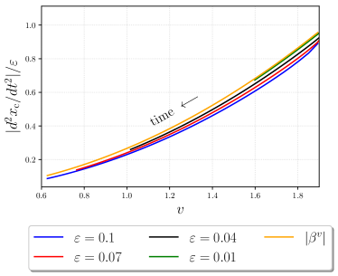
Figure 13: Using the kinematic definition of the peak velocity, we reconstruct the beta function from the peak position of the full solution $\varphi_{\text{full}}$, at different values of $\varepsilon$ (using Eq. (129)). These converge to the DRG-computed $|\beta^{v}|$ (extracted in Sec. IV.1) as $\varepsilon$ becomes smaller. We note that if the horizontal axis is reparameterized to be $v-\varepsilon\alpha^{v}_{\text{full}}(v)$, all of the curves coincide.

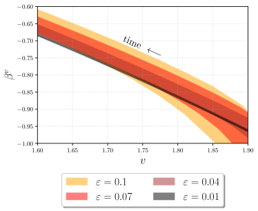
Figure 14: Convergence of the beta function curves in Eqs. (129-131) built from the different shape parameters. The colored regions, containing all of the alternative forms of the beta function, expand as $\varepsilon$ becomes larger.

We can similarly numerically extract $\beta^{v}$ from time derivatives of $\mathcal{W}_{\text{full}}$ and $\mathcal{A}_{\text{full}}$. From Eq. (124), we should have

$$\beta_{\text{full}}^{v}\approx-\frac{\varepsilon^{-1}}{2\cosh^{-1}\sqrt{2}}v_{\text{full}}^{3/2}\frac{d\mathcal{W}_{\mathrm{full}}}{dt}\,.$$ (130)

Here the approximate equality is due to the peaks of the full solution not being symmetric. Similarly, from the original parameterization of the amplitude, we should have

$$\beta_{\text{full}}^{v}=\frac{2}{\varepsilon}\frac{d\mathcal{A}_{\mathrm{full}}}{dt},$$ (131)

which is also seen in Eq. (112).

In Fig. 14, we plot the spread of the curves representing all of the “equivalent” forms of $\beta^{v}$ [from Eq. (129), (130), and Eq. (131)]. For each choice of $\varepsilon$, we shaded the areas containing all of the curves with a different color. Notice that the curves tend to spread more as $\varepsilon$ becomes larger, and therefore the colored regions grow in the same manner. As before, the case $\varepsilon=0.01$ limits the range of velocities, and determines the size of the horizontal axis in which all the regions can be compared. The DRG-extracted value of $\beta^{v}$ (yellow curve in Fig. 13) overlaps with the region shaded in black in Fig. 14 after reparameterizing the horizontal axis with $\alpha^{v}_{\text{full}}$. Therefore this result is consistent with the system being described by the two-dimensional flow, as seen in Sec. IV.2.

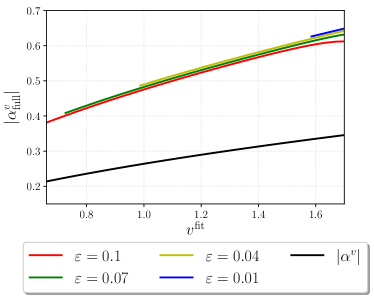
Figure 15: Mismatch between $\alpha^{v}$, extracted using the DRG, and $\alpha^{v}_{\text{full}}$, extracted by fitting the full solution (at four different values of $\varepsilon$). There is an unexplained ratio of approximately 2 between them.

We can also determine $\alpha_{\text{full}}^{v}$ from $\varphi_{\text{full}}$. To do so, we parameterize each time snapshot of the full solution of Eq. (69) as

$$\varphi_{\mathrm{full}}=\frac{v^{\mathrm{fit}}}{2}\operatorname{sech}^{2}\left[\frac{\sqrt{v^{\mathrm{fit}}}}{2}(x-x^{\mathrm{fit}}_{\mathrm{c}})\right]\,,$$ (132)

and fit $v^{\mathrm{fit}}$ and $x^{\mathrm{fit}}_{\mathrm{c}}$ using curve_fit. We can reconstruct the reparameterization $\alpha_{\text{full}}^{v}$ by computing the difference

$$|\alpha_{\mathrm{full}}^{v}|=\frac{1}{\varepsilon}\bigg{|}v^{\mathrm{fit}}-\frac{dx^{\mathrm{fit}}_{\mathrm{c}}}{dt}\bigg{|}\,.$$ (133)

That is, the reparameterization captures the difference between the kinematical velocity $dx^{\text{fit}}/dt$ versus the shape parameter named $v^{\text{fit}}$. In Fig. 15, we plot this quantity versus the DRG-extracted value of $\alpha^{v}$ (in the right panel of Fig. 8). Our results show that there is no convergence towards the renormalized alpha function as $\varepsilon\rightarrow 0$, as in the case for the beta function $\beta^{v}$. The slope seems to be correct, but the value of the alpha function extracted using our renormalization procedure is smaller than $|\alpha^{v}_{\mathrm{full}}|$ by a factor of 2. If we use $\alpha^{v}_{\text{full}}$ as a shift in the initial velocity to reconstruct the renormalized solution, we notice a slight reduction in the relative error, compared to what is reported in the right panel of Fig. 9. We do not currently understand the origin of this difference. We leave the resolution of this mismatch for a future project.

V Potential applications

As already surveyed in several textbooks [4, 5, 2, 3] and articles [9, 19, 21], there are a wide range of physical problems where secular effects need to be captured properly. The DRG unifies several approaches to secular perturbation theory and can thus be applied to any such secular problem. We expect our addition of a numerical formulation of DRG will further extend its applicability to include problems which can only be solved numerically. One potential application is to compute the beta functions for long-lived cosmological solutions, such as oscillons [40, 41, 42, 43, 44, 45]. It might be possible to produce oscillons (quasibreathers) from continuous deformations of the sine-Gordon breather [46]. Concretely, our method can be applied to find an estimated lifetime of such oscillons.

Our original motivation to implement the numerical DRG arose from a certain problem in gravitational physics. We are interested in the gravitational waves emitted by black hole binary systems. As we have already seen in Sec. II.1, the post-Newtonian regime (where $1/c$ is a perturbation parameter) can be treated using the DRG analytically. As an update of the results in [31], the work of Yang and Leibovich uses the DRG to include spin-orbit effects in the inspiral [47]. The extreme mass-ratio inspiral (EMRI) problem [48], which is treated perturbatively in powers of the small mass ratio, should also be amenable to the DRG. There are several secular timescales in the EMRI problem, all of which need to be controlled (see e.g. [49]).

The specific problem of interest is in how the inspiral and resulting gravitational waves are modified by the presence of corrections to Einstein’s theory of general relativity [50]. For most beyond-GR theories, the status of the initial value problem is open, though it is expected that most of these theories lack a good initial value formulation [51]. Instead, the only sound way to treat such a theory is as a perturbation around GR, where a parameter $\varepsilon$ controls the strength of the deformation away from GR; this is the viewpoint of effective field theory (however, for a different nonperturbative proposal, see [52, 53, 54]). This is also in line with observations, which to date are consistent with the predictions of general relativity [55].

Indeed, treating beyond-GR theories as perturbations to GR has been successful for finding stationary solutions [56, 57], where there are no secular effects; and even for addressing the post-Newtonian regime of the binary inspiral problem, which does suffer from secular effects (Refs. [58, 57] treated these secular effects with traditional secular perturbation theory, rather than the DRG).

The challenge now is to handle the late inspiral and merger phase of a binary black hole system in a beyond-GR theory such as dynamical Chern-Simons gravity (dCS) [59]. The merger phase can only be treated with full numerical relativity, not by any analytical means. The beyond-GR perturbation is similarly treated numerically, expanded about the nonlinear GR solution [60, 61, 62, 63]. This perturbative solution however suffers from secular growth, as predicted in [60] and confirmed in [61, 62, 63]. Similarly, secular growth appears when applying naive perturbation theory to Einstein-dilaton-Gauss-Bonnet gravity [63].

The origin of this secular growth is easy to understand. The background (GR) solution inspirals at a particular rate; the correction to GR includes a change in the energy radiated, thus changing the rate of inspiral. This also has a simple analogy with the KdV equation, which motivated this study. Both the KdV problem and the binary black hole inspirals in GR have nonlinear background solutions, and these background solutions both have non-vanishing flows $\vec{\beta}^{(0)}$. In both cases, the perturbation removes energy from the system, causing the true speed (of the soliton or inspiral) to deviate from the background speed.

It is this secular growth that we seek to control. As a reminder, the initial-value problem for most beyond-GR theories can only be formulated in naive perturbation theory. Below we sketch this naive perturbation theory approach, which breaks down, and then how the numerical DRG will be used to renormalize the secularly-growing solutions. We do not claim that this is the only or the best approach to this problem. Indeed if there was another viable approach available (e.g. that proposed in [52, 53, 54]), it would be prudent to compare the independent methods to assess their merits. However, no other general-purpose approach is available which has been shown to simulate arbitrary beyond-GR theories.

The equations of motion of such beyond-GR theories can be cast as a deformation of Einstein’s field equations,

$$G_{ab}+\varepsilon C_{ab}=8\pi T_{ab}\,,$$ (134)

where $C_{ab}$ is generating the correction to GR, and is controlled by the parameter $\varepsilon$. The metric is expanded as an ordinary perturbation series,

$$g_{ab} =g^{(0)}_{ab}+\varepsilon g^{(1)}_{ab}+\mathcal{O}(\varepsilon^{2})\,,$$ (135)

and similarly for any other degrees of freedom. The background solution $g^{(0)}_{ab}$ satisfies the nonlinear Einstein field equations (and already contains gravitational waves). The correction due to beyond-GR effects, $g^{(1)}_{ab}$, satisfies the linearization of Eq. (134) and can be integrated alongside $g^{(0)}_{ab}$, as was first demonstrated in [61]. It is this $g^{(1)}_{ab}$ which suffers from secular growth, as seen in [62].

Let us review the ingredients needed to implement the numerical DRG in this case. The first necessary condition is that the problem can be described by a finite-dimensional attractor manifold. This may not be clear since GR is a field theory and thus has an infinite number of degrees of freedom. But, as long as the initial data is close to a binary of black holes, any small gravitational fluctuations will radiate away rapidly, leaving a system with a finite-dimensional solution manifold, parameterized by the two black holes’ masses, spins, and separation (here we ignore eccentricity). In this finite-dimensional parameter space $\Lambda$, so-called surrogate models [64, 65] have been highly successful in giving a faithful numerical model for the asymptotic waveform at infinity, which we will denote as simply

$$h^{\text{Surr}}[\vec{\lambda}]\,,$$ (136)

where $\vec{\lambda}\in\Lambda$ are the system parameters. This quantity may come from a spline interpolant (or other reduced order model), and therefore we also have access to the differentials

$$\frac{\delta h^{\text{Surr}}}{\delta\vec{\lambda}}\,,$$ (137)

which are then also spline interpolants. The parameters $\vec{\lambda}$ already experience a background flow, $d\vec{\lambda}/dt=\vec{\beta}^{(0)}(\vec{\lambda})$, since the binary inspirals, and the spins (and orbit) precess. Using this background flow, we can build the infinitesimal flow $\vec{V}$ using the BCH theorem, and thus have a model for $h^{(1)}_{\parallel}$, the secularly-growing part of $g^{(1)}_{ab}$, in terms of the first-order $\vec{\alpha}^{(1)}$ and $\vec{\beta}^{(1)}$. Finally, since we have access to the numerical first-order solution $g^{(1)}_{ab}$, we fit the model $h^{(1)}_{\parallel}$, getting numerical $\vec{\alpha}^{(1)}$ and $\vec{\beta}^{(1)}$ as fit parameters, for some individual beyond-GR simulation. After fitting, we also have the residuals $h^{(1)}_{\perp}$.

If we repeat the fit for many beyond-GR simulations, we can then interpolate $\vec{\alpha}^{(1)}$ and $\vec{\beta}^{(1)}$. Finally, we can solve the deformed flow equations

$$\frac{d\vec{\lambda}_{\text{R}}}{dt}=\vec{\beta}^{(0)}+\varepsilon\vec{\beta}^{(1)}\,,$$ (138)

to find $\vec{\lambda}_{\text{R}}(t)$. This renormalized flow captures the different rate of inspiral due to the beyond-GR effects. Finally, we can evaluate the renormalized asymptotic waveforms,

$$h_{\text{R}}=h^{\text{Surr}}[\vec{\lambda}_{\text{R}}(t)]\,,$$ (139)

which do not suffer any secular effects. Although this captures most of the beyond-GR effects, there are still $\mathcal{O}(\varepsilon)$ “instantaneous” corrections in $h^{(1)}_{\perp}$, which should also be incorporated.

VI Discussion

In this paper, we proposed a systematic numerical method to applying the dynamical renormalization group to finite- or infinite-dimensional dynamical systems, even in situations when analytical perturbation theory is not possible. To make this possible, we formulated the DRG in the language of differential geometry, in Sec. II.2. From the geometric point of view, naive perturbation theory finds tangent vectors in solution space, which are then integrated together to find the whole DRG flow. This geometric formulation is general enough that the DRG can be applied to systems that already have a background flow in parameter space, so that the DRG may be iterated to higher order.

As a proof of concept, in Sections III and IV, we applied this method to the Korteweg-de Vries equation, deforming it to the Korteweg-de Vries-Burgers equation. We used naive perturbation theory, numerically, and as expected, found secularly-growing solutions. We fit these solutions using appropriate basis functions, which are computed from derivatives of the background solution with respect to parameters, $\delta\varphi^{(0)}/\delta\vec{\lambda}$, along with knowledge of the background flow $\vec{\beta}^{(0)}$. By minimizing an appropriate cost functional, we extract values of the generators $\vec{\alpha}^{(1)}$ and $\vec{\beta}^{(1)}$, for each numerical simulation. Just finding these values already gives deep information about the structure of parameter space. Now one can numerically solve the deformed parameter flow $d\vec{\lambda}_{\text{R}}/dt=\vec{\beta}^{(0)}+\varepsilon\vec{\beta}^{(1)}$, for example by interpolating through parameter space. Finally we find the renormalized solution $\varphi^{(0)}[\vec{\lambda}_{\text{R}}(t)]$.

This example highlights a number of key features of the numerical DRG approach. Most importantly, we have controlled the secular divergence on the shortest timescale in the problem, $T_{\text{sec}}\sim\varepsilon^{-1/2}$. The numerical beta function we extracted is highly suggestive of a power law $\propto v^{2}$, in agreement with an analytical calculation suggested by [37] (a numerical fit to the power law index differs only in the fourth decimal place). Despite the excellent agreement in the beta function, the reparameterization generator $\alpha^{v}$ seems to disagree with an independent check we performed in Sec. IV.3. Nonetheless, even using this wrong value of $\alpha$ gives results that are better than using no $\alpha$ reparameterization at all, and the solution is still valid on secularly long times. Finally, in Sec. IV.2 we demonstrated how to test if the perturbation has increased the dimensionality of the parameter space, by considering a more general parameterization to the one-soliton KdV solution. For the KdV problem, we found that solutions lie in a submanifold with the original dimensionality, so dimensionality was not increased.

There are a plethora of potential applications for the numerical DRG. We discussed some possibilities in Sec. V, including finding oscillon lifetimes, secular divergences in extreme mass-ratio inspirals, and gravitational waves from beyond-GR theories. There are also still unanswered questions raised by the KdV example of this work. For example, we do not yet understand the apparent factor of two discrepancy in the $\alpha$ function, found in Sec. IV.3. Our example demonstrated control of the secular effects, which are most important for the breakdown of perturbation theory, but there are also “instantaneous” perturbative effects that we did not include. We noticed in Sec. IV.1 that both the residual $\varphi^{(1)}_{\perp}$ and the true solution $\varphi_{\text{full}}$ contain “diluting tails.” However in this work we restricted attention to the renormalization procedure and the solution $\varphi_{\text{ren}}=\varphi^{(0)}(\vec{\lambda}_{\text{R}}(t))$, so we made no effort to capture the $\mathcal{O}(\varepsilon)$ instantaneous effects. The formalism to include information from $\varphi^{(1)}_{\perp}$ still needs to be developed.

Appendix A Numerical setup and errors in the alpha and beta functions

In this Appendix, we describe the numerical setup to evolve the first-order perturbations of the KdV equation in Eq. (75) and the full KdVB equation in Eq. (69). We followed a standard algorithm described by Boyd [39] to solve the KdVB equation, and depicted it in Fig. 16. This is pseudospectral in space, using the Fourier basis, and the method of lines for time evolution. The essence of this algorithm is to compute the time derivative by finding real-space operations (like products) in the collocation basis, but computing any derivatives in the spectral domain, and afterwards transform back to the collocation domain for time evolution. We use fftw3 [66] in our implementation to perform fast Fourier transforms (FFTs) and their inverses. As every spectral approach, working in the Fourier domain has several benefits:

• It simplifies the representation of spatial derivatives as multiplying by powers of the wavevector $k$.

• It does not require any explicit preparation of boundary conditions since these are periodic by definition.

• The output data allows spectrally accurate operations, such as spatial differentiation, integration along the x-axis, and interpolation.

We exploited all of these advantages during the post-processing phase of our simulation results. It is also possible to build a code with perfectly matched layers, in addition to periodic boundary conditions. This procedure prevents the re-entry of fast/high frequency modes in the simulation box after transforming oscillatory modes into decaying modes by analytic continuation [67]. We will use such an implementation in a future project.

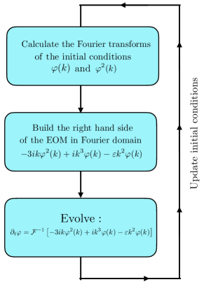
Figure 16: Simplified scheme showing the solution algorithm for the KdVB equation in Eq. (69), the solution for the perturbation $\varphi^{(1)}$ follows a similar process. The symbol $\mathcal{F}^{-1}$ denotes the inverse Fourier transform.

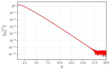
Figure 17: Left panel: Power spectrum of $\varphi_{\mathrm{full}}$ at $t=50$, corresponding to the final snapshot of the numerical evolution from Eq. (69). We considered a KdV soliton as an initial condition with $v=2$. Right panel: Power spectrum of the perturbation solution of Eq. (75) at $T_{\max}=300$, where the background is a $v=2$ soliton. In both panels, we observe that the high frequency contribution remains in the levels of round-off errors in double precision.

We use the method of lines for the collocation data to evolve in the time domain. Our time integration routine is an explicit eighth-order accurate Gauss-Legendre integrator [68], which is A-stable and symplectic for Hamiltonian problems. In order to understand the time scales involved, we write the space and time Fourier transform of the linear operator $\mathrm{KdV}^{(1)}$, with “frozen coefficients,” to derive the high-frequency dispersion relation from the homogeneous part of Eq. (75),

$$\omega\varphi^{(1)}_{k}=\left[6k\varphi^{(0)}+6i\partial_{x}\varphi^{(0)}-k^{3}\right]\varphi^{(1)}_{k},$$ (140)

where the background and its derivatives are smooth and bounded functions. For $v<10$, the dominant contribution to the dispersion relation comes from the third spatial derivative (the contribution of the two other terms is comparable to $k^{3}$ only when $v\geq 10$). Therefore we find the time step for evolution is limited by the Courant-Friedrichs-Lewy condition, in this case,

$$\Delta t_{\mathrm{CFL}}\approx\frac{1}{k_{\max}^{3}}.$$ (141)

As there are real and imaginary parts of the frequency, we can observe the presence of attenuated oscillatory modes propagating to the left with a phase velocity proportional to $k^{2}$. It is important to notice their presence since it is possible for these modes to travel and propagate through the periodic domain and deform the solitonic peak and the perturbative solution. If it is not controlled, the propagation of these oscillatory modes introduces oscillations in all the evolution plots of the shape parameters shown in Figs. 12 and 13. In order to avoid or minimize those effects, we use a large simulation domain with length $L=2560$ to allow the attenuation of oscillatory modes as these propagate.

From the solitonic initial condition in Eq. (72) we notice that as the parameter $v$ grows, the peak becomes more acute and hence the solution has more power in higher frequencies. This not only results in smaller time steps for resolving the system correctly, but the solution becomes prone to develop high-frequency instabilities. Thus, the selection of the range of parameter values for $v$ demands us to proceed with caution. The largest $v$ probed in our study is $v=2$. In the left panel of Fig. 17, we plot the power spectrum of the final snapshot at $t=50$ of the full KdVB solution. Here we used the KdV soliton in Eq. (72) with $v=2$ as the initial condition. In the right panel, we plot the power spectrum at $T_{\max}=300$ for the perturbative solution, where the background is a KdV soliton with $v=2$, and the initial conditions for the perturbation vanish at time $t=0$. The floor at high-frequencies corresponds to round-off error at the level of machine precision, showing that our results are free of high-frequency instabilities. Still, the convergence error grows with $v$, as can be seen in Table 1.

	$v\geq 0.5$		$v<0.5$
Resolutions	$\Delta t$	# of nodes	$\Delta t$	# of nodes
high (hi)	$0.00005$	$2^{14}$	$0.0001$	$2^{14}$
mid (mi)	$0.0001$	$2^{14}$	$0.001$	$2^{13}$
low (low)	$0.001$	$2^{13}$	$0.002$	$2^{13}$
ultra-low (ult.low)	$0.002$	$2^{13}$	$0.01$	$2^{12}$

Table 3: Resolutions and their corresponding values for the time step and the number of collocation points in Fourier grid. These are the same resolution levels used to produce the convergence errors represented in Fig. 8.

Depending on the resolution, we used either $N=2^{12}$, $N=2^{13}$, or $N=2^{14}$ collocation nodes on an equally spaced Fourier grid. We calculated the perturbative solution $\varphi^{(1)}$ at four different resolutions specified in Table 3 with the purpose of finding the convergence errors for all the extracted alpha and beta values. In the range of $v<0.5$, where the solution peaks are wider and have a slower propagation, it is convenient to shift the resolutions to also consider $2^{12}$ collocation points with a time-step $\Delta t=0.01$. As can seen in the table, in the range of $v<0.5$, such a new configuration becomes the ultra low resolution, the “u-low” case for $v\geq 0.5$ is now the “low” resolution and each of the remaining resolutions for $v\geq 0.5$ are promoted to be the next highest resolution for $v<0.5$.

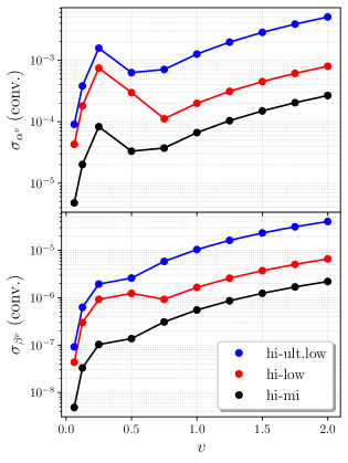
Figure 18: Convergence plots for $\alpha^{v}$ and $\beta^{v}$ as functions of the solution parameter $v$. The differences between the values of $\beta^{v}$ and $\alpha^{v}$ reduce as the quantities are extracted from better resolved datasets. The differences $\sigma_{\alpha^{v}}$ and $\sigma_{\beta^{v}}$, reported in Table 1, correspond to the error curves in red.

Extracting the values of the beta functions requires spatial integration of the coefficients in Eqs. (95) and (96) along the full simulation domain, which can be computed spectrally accurately by using the Fourier transform,

$$\int_{-L/2}^{L/2}f(x)dx=L\,\tilde{f}(k=0)\,,$$ (142)

where $\tilde{f}(k)$ is the Fourier transform of the integrand. For the time integrals we used the standard Simpson integration rule, which is second-order accurate.

All the derivatives of the background solution (i.e., $\delta\varphi^{(0)}/\delta\lambda^{i}$) reported in this paper are computed from analytic expressions, and thus do not introduce errors in the extraction. From the evaluation of the expressions in Eq. (97) at different resolutions, it is possible to calculate the alpha and beta functions using Eq. (68) at each resolution for every tabulated value of the varying parameter. The convergence errors reported in Table 1 (dubbed as $\sigma_{\alpha^{v},\beta^{v}}~{}(\text{conv.})$) were computed as follows. First, we compute $\alpha$ and $\beta$ at all the resolutions in Table 3. Secondly, we calculate the differences of the values of $\alpha^{v}$ and $\beta^{v}$ extracted at the highest resolution with the corresponding values at the other three lower resolutions. These differences are plotted in Fig. 18. Notice that the errors decrease as the resolution increases, forming a clear convergence pattern for all values of $v$. To be extremely conservative, we used the difference hi-low, plotted in red in Fig. 18, as the convergence errors. The vast majority of the values shown in Fig. 18 are significantly smaller than the RE error reported in Table 1. These values were plotted as a complement to the results visible in the lower panels of Fig. 8, showing in detail the convergence errors $\sigma_{\alpha^{v}}~{}\text{(conv.)}$ and $\sigma_{\beta^{v}}~{}\text{(conv.)}$ evaluated at different resolutions. In the future, we may instead perform independent Richardson extrapolation at each resolution; and then check convergence of the Richardson extrapolants across resolutions.

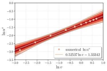
Figure 19: Using an enlarged version of the covariance matrix in Eq. (102) (multiplied by $500$), we represent the region where the extracted alpha function can be found.

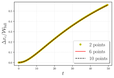
Figure 20: Comparing the peak position of the renormalized solution with the peak position of $\varphi_{\mathrm{full}}$ in a ratio with the width. The renormalized solution is generated by picking 2, 6, and 10 different values of $\beta^{v}$ from Table 1 and $\alpha^{v}|_{v=2}$ at $\varepsilon=0.1$ to reparameterize the initial velocity. Changing the number of points does not introduce any significant difference in the error variable $\Delta x_{\text{c}}/\mathcal{W}_{\text{full}}$.

The values of $\alpha^{v}$, $\beta^{v}$, and their Richardson extrapolation errors all entered into the power law fits, producing the optimal values in Table 2 and estimated “covariance matrices” in Eqs. (102) and (103). These are not statistical covariances, all being due to systematic errors; nonetheless we can interpret them as Gaussian distributions in order to show the region of the $(\ln v,\ln\alpha^{v})$ plane where the true $\alpha^{v}$ may be found. This is plotted in Fig. 19, using the package fgivenx [69]. To produce a visible output, it was necessary to multiply the covariance matrix by a factor of $500$ for $\ln\alpha^{v}$. The same can be applied to find the possible region for $\beta^{v}$ in the $(\ln v,\ln|\beta^{v}|)$ plane, in the context of a pure power law $\beta$ function.

In the right panel of Fig. 9, for $\varepsilon=0.1$, we observe that the greatest difference between the renormalized and the full solution comes from a shift in the peak position $x_{\mathrm{c}}$. Here we test whether this is due to errors in our fits for $\alpha^{v}$ and $\beta^{v}$, or due to truncation errors in the time integration when solving the numerical DRG equations for $(v_{\text{R}}(t),x^{\text{R}}_{c}(t))$. To assess the importance of truncation error in the DRG time integration, we performed the integration with $\Delta t=0.5,~{}0.01$ and $0.001$, using the same underlying power-law fits for $\alpha^{v}$ and $\beta^{v}$ as reported in Table 2. We did not observe any visible differences between the outcomes for the different time step choices. This is a clear indication of the subdominance of the integration error. To assess if the power law fit errors are under-reported, we changed the number of points for fitting $\ln|\beta^{v}|$ as a linear function of $\ln v$. The left panel of Fig. 8 already provides enough evidence of the linear relation between these variables. Therefore, in principle we only require two points of the sample in Table 1 to determine the coefficients $m$ and $b$. We reconstructed $\beta^{v}$ as a function of $v$ choosing two, six, and ten of the points in the table (the points $v=0.125$ and $v=2$ are considered in all three cases, we did not include the extremum $v=0.0625$ in the case with 2 points since it has the largest relative error). We then integrated the coupled system in Eqs. (105) and (106) for all of the beta functions generated by each of these choices, and plot the results in Fig. 20 (normalized by the width $\mathcal{W}_{\text{full}}$, computed as in Sec. IV.3). The results are not affected by changing the number of points included in the fit, again suggesting that the fits are not the responsible for the error $\Delta x_{c}$. Having ruled out either of these possibilities, we suspect that the main source of this error comes from the mismatch between $\alpha^{v}$ and $\alpha^{v}_{\text{full}}$ discussed in Sec. IV.3.

References

- Coleman [2018] S. Coleman, Lectures of Sidney Coleman on Quantum Field Theory, edited by B. G.-g. Chen, D. Derbes, D. Griffiths, B. Hill, R. Sohn, and Y.-S. Ting (WSP, Hackensack, 2018).
- Bender and Orszag [1999] C. Bender and S. Orszag, Advanced Mathematical Methods for Scientists and Engineers I: Asymptotic Methods and Perturbation Theory, Advanced Mathematical Methods for Scientists and Engineers (Springer, 1999).
- Kevorkian and Cole [1981] J. Kevorkian and J. Cole, Perturbation Methods in Applied Mathematics, Applied Mathematical Sciences (Springer, 1981).
- Goldstein et al. [2002] H. Goldstein, C. Poole, and J. Safko, Classical Mechanics (Addison Wesley, San Francisco, 2002).
- José and Saletan [1998] J. V. José and E. J. Saletan, Classical Dynamics: A Contemporary Approach (Cambridge University Press, 1998).
- Abrikosov [1957] A. Abrikosov, The magnetic properties of superconducting alloys, Journal of Physics and Chemistry of Solids 2, 199 (1957).
- Goldenfeld [1992] N. Goldenfeld, Lectures on phase transitions and the renormalization group (CRC Press, Boca Raton, 1992).
- Chen and Goldenfeld [1995] L.-Y. Chen and N. Goldenfeld, Numerical renormalization-group calculations for similarity solutions and traveling waves, Phys. Rev. E 51, 5577 (1995).
- Chen et al. [1996] L.-Y. Chen, N. Goldenfeld, and Y. Oono, The Renormalization group and singular perturbations: Multiple scales, boundary layers and reductive perturbation theory, Phys. Rev. E 54, 376 (1996), arXiv:hep-th/9506161 .
- Bellac and Barton [1991] M. Bellac and G. Barton, Quantum and Statistical Field Theory, Oxford Science Publ (Clarendon Press, 1991).
- Als-Nielsen and Birgeneau [1977] J. Als-Nielsen and R. J. Birgeneau, Mean field theory, the Ginzburg criterion, and marginal dimensionality of phase transitions, American Journal of Physics 45, 554 (1977).
- Dyson [1952] F. J. Dyson, Divergence of perturbation theory in quantum electrodynamics, Phys. Rev. 85, 631 (1952).
- Kadanoff [1977] L. P. Kadanoff, Lectures on the Application of Renormalization Group Techniques to Quarks and Strings, International School on Statistical Mechanics: Critical Phenomena Sitges, Spain, May 23-June 5, 1976, Rev. Mod. Phys. 49, 267 (1977).
- Weinberg [2005] S. Weinberg, The Quantum theory of fields. Vol. 1: Foundations (Cambridge University Press, 2005).
- Misner et al. [1973] C. W. Misner, K. S. Thorne, and J. A. Wheeler, Gravitation (W. H. Freeman, San Francisco, 1973).
- Mukhanov et al. [1992] V. F. Mukhanov, H. A. Feldman, and R. H. Brandenberger, Theory of cosmological perturbations. Part 1. Classical perturbations. Part 2. Quantum theory of perturbations. Part 3. Extensions, Phys. Rept. 215, 203 (1992).
- Ma and Bertschinger [1995] C.-P. Ma and E. Bertschinger, Cosmological perturbation theory in the synchronous and conformal Newtonian gauges, Astrophys. J. 455, 7 (1995), arXiv:astro-ph/9506072 [astro-ph] .
- Burgess et al. [2010] C. P. Burgess, L. Leblond, R. Holman, and S. Shandera, Super-Hubble de Sitter Fluctuations and the Dynamical RG, JCAP 03, 033, arXiv:0912.1608 [hep-th] .
- Kunihiro [1995] T. Kunihiro, A Geometrical formulation of the renormalization group method for global analysis, Prog. Theor. Phys. 94, 503 (1995), [Erratum: Prog.Theor.Phys. 95, 835 (1996)], arXiv:hep-th/9505166 .
- Kuramoto [1989] Y. Kuramoto, On the Reduction of Evolution Equations in Extended Systems, Progress of Theoretical Physics Supplement 99, 244 (1989).
- Ei et al. [2000] S.-I. Ei, K. Fujii, and T. Kunihiro, Renormalization group method for reduction of evolution equations: Invariant manifolds and envelopes, Annals Phys. 280, 236 (2000), arXiv:hep-th/9905088 [hep-th] .
- Higashijima and Nishijima [1980] K. Higashijima and K. Nishijima, Renormalization Groups of Gell-mann-low and of Callan-symanzik, Prog. Theor. Phys. 64, 2179 (1980).
- Callan [1970] C. G. Callan, Jr., Broken scale invariance in scalar field theory, Phys. Rev. D 2, 1541 (1970).
- Symanzik [1971] K. Symanzik, Small distance behavior analysis and Wilson expansion, Commun. Math. Phys. 23, 49 (1971).
- Symanzik [1970] K. Symanzik, Small distance behavior in field theory and power counting, Commun. Math. Phys. 18, 227 (1970).
- [26] J. Bricmont and A. Kupiainen, Renormalizing partial differential equations (Springer Berlin Heidelberg) pp. 83–115, chao-dyn/9411015 .
- Betelú et al. [2000] S. Betelú, D. Aronson, and S. Angenent, Renormalization study of two-dimensional convergent solutions of the porous medium equation, Physica D: Nonlinear Phenomena 138, 344–359 (2000), patt-sol/9908006 .
- Braga et al. [2020] G. a. A. Braga, F. Furtado, V. Isaia, and L. Lee, Numerical renormalization group algorithms for self-similar asymptotics of partial differential equations, Multiscale Modeling & Simulation 18, 131 (2020).
- Canosa and Gazdag [1977] J. Canosa and J. Gazdag, The Korteweg-de Vries-Burgers equation, Journal of Computational Physics 23, 393 (1977).
- Olver [1993] P. Olver, Applications of Lie groups to differential equations, Graduate texts in mathematics (Springer-Verlag, 1993).
- Galley and Rothstein [2017] C. R. Galley and I. Z. Rothstein, Deriving analytic solutions for compact binary inspirals without recourse to adiabatic approximations, Phys. Rev. D95, 104054 (2017), arXiv:1609.08268 [gr-qc] .
- Kuehn [2015] C. Kuehn, Multiple Time Scale Dynamics, Applied Mathematical Sciences (Springer, 2015).
- Lee [2013] J. M. Lee, Smooth manifolds, in Introduction to Smooth Manifolds (Springer, New York, NY, 2013).
- Achilles and Bonfiglioli [2012] R. Achilles and A. Bonfiglioli, The early proofs of the theorem of Campbell, Baker, Hausdorff, and Dynkin, Archive for history of exact sciences 66, 295 (2012).
- Richardson [1911] L. F. Richardson, The approximate arithmetical solution by finite differences of physical problems involving differential equations, with an application to the stresses in a masonry dam, Philosophical Transactions of the Royal Society of London. Series A, Containing Papers of a Mathematical or Physical Character 210, 307 (1911).
- Press et al. [1992] W. H. Press, S. A. Teukolsky, W. T. Vetterling, and B. P. Flannery, Numerical Recipes in FORTRAN: The Art of Scientific Computing.
- Tu and Cheng [2002] T. Tu and G. Cheng, Renormalization group theory for perturbed evolution equations, Phys. Rev. E 66, 046625 (2002), cond-mat/0106087 .
- Virtanen et al. [2020] P. Virtanen, R. Gommers, T. E. Oliphant, M. Haberland, T. Reddy, D. Cournapeau, E. Burovski, P. Peterson, W. Weckesser, J. Bright, S. J. van der Walt, M. Brett, J. Wilson, K. J. Millman, N. Mayorov, A. R. J. Nelson, E. Jones, R. Kern, E. Larson, C. J. Carey, İ. Polat, Y. Feng, E. W. Moore, J. VanderPlas, D. Laxalde, J. Perktold, R. Cimrman, I. Henriksen, E. A. Quintero, C. R. Harris, A. M. Archibald, A. H. Ribeiro, F. Pedregosa, P. van Mulbregt, and SciPy 1.0 Contributors, SciPy 1.0: Fundamental Algorithms for Scientific Computing in Python, Nature Methods 17, 261 (2020).
- Boyd [2001] J. P. Boyd, Chebyshev and Fourier Spectral Methods (Dover Publications, Mineola, NY, 2001).
- Amin et al. [2012] M. A. Amin, R. Easther, H. Finkel, R. Flauger, and M. P. Hertzberg, Oscillons After Inflation, Phys. Rev. Lett. 108, 241302 (2012), arXiv:1106.3335 [astro-ph.CO] .
- Lozanov and Amin [2019] K. D. Lozanov and M. A. Amin, Gravitational perturbations from oscillons and transients after inflation, Phys. Rev. D 99, 123504 (2019), arXiv:1902.06736 [astro-ph.CO] .
- Amin et al. [2018] M. A. Amin, J. Braden, E. J. Copeland, J. T. Giblin, C. Solorio, Z. J. Weiner, and S.-Y. Zhou, Gravitational waves from asymmetric oscillon dynamics?, Phys. Rev. D 98, 024040 (2018), arXiv:1803.08047 [astro-ph.CO] .
- Ollé et al. [2021] J. Ollé, O. Pujolàs, and F. Rompineve, Recipes for oscillon longevity, Journal of Cosmology and Astroparticle Physics 2021 (09), 015.
- Zhang et al. [2020] H.-Y. Zhang, M. A. Amin, E. J. Copeland, P. M. Saffin, and K. D. Lozanov, Classical Decay Rates of Oscillons, JCAP 07, 055, arXiv:2004.01202 [hep-th] .
- Cyncynates and Giurgica-Tiron [2021] D. Cyncynates and T. Giurgica-Tiron, Structure of the oscillon: The dynamics of attractive self-interaction, Phys. Rev. D 103, 116011 (2021), arXiv:2104.02069 [hep-ph] .
- Ablowitz et al. [1973] M. J. Ablowitz, D. J. Kaup, A. C. Newell, and H. Segur, Method for solving the sine-Gordon equation, Phys. Rev. Lett. 30, 1262 (1973).
- Yang and Leibovich [2019] Z. Yang and A. K. Leibovich, Analytic Solutions to Compact Binary Inspirals With Leading Order Spin-Orbit Contribution Using The Dynamical Renormalization Group, Phys. Rev. D 100, 084021 (2019), arXiv:1908.05688 [gr-qc] .
- Poisson et al. [2011] E. Poisson, A. Pound, and I. Vega, The Motion of point particles in curved spacetime, Living Rev. Rel. 14, 7 (2011), arXiv:1102.0529 [gr-qc] .
- Miller and Pound [2021] J. Miller and A. Pound, Two-timescale evolution of extreme-mass-ratio inspirals: waveform generation scheme for quasicircular orbits in Schwarzschild spacetime, Phys. Rev. D 103, 064048 (2021), arXiv:2006.11263 [gr-qc] .
- Berti et al. [2015] E. Berti et al., Testing General Relativity with Present and Future Astrophysical Observations, Class. Quant. Grav. 32, 243001 (2015), arXiv:1501.07274 [gr-qc] .
- Lehner and Pretorius [2014] L. Lehner and F. Pretorius, Numerical Relativity and Astrophysics, Ann. Rev. Astron. Astrophys. 52, 661 (2014), arXiv:1405.4840 [astro-ph.HE] .
- Cayuso et al. [2017] J. Cayuso, N. Ortiz, and L. Lehner, Fixing extensions to general relativity in the nonlinear regime, Phys. Rev. D 96, 084043 (2017), arXiv:1706.07421 [gr-qc] .
- Allwright and Lehner [2019] G. Allwright and L. Lehner, Towards the nonlinear regime in extensions to GR: assessing possible options, Class. Quant. Grav. 36, 084001 (2019), arXiv:1808.07897 [gr-qc] .
- Cayuso and Lehner [2020] R. Cayuso and L. Lehner, Nonlinear, noniterative treatment of EFT-motivated gravity, Phys. Rev. D 102, 084008 (2020), arXiv:2005.13720 [gr-qc] .
- Abbott et al. [2019] B. P. Abbott et al. (LIGO Scientific, Virgo), Tests of General Relativity with the Binary Black Hole Signals from the LIGO-Virgo Catalog GWTC-1, Phys. Rev. D 100, 104036 (2019), arXiv:1903.04467 [gr-qc] .
- Yunes and Stein [2011] N. Yunes and L. C. Stein, Non-Spinning Black Holes in Alternative Theories of Gravity, Phys. Rev. D 83, 104002 (2011), arXiv:1101.2921 [gr-qc] .
- Yagi et al. [2013] K. Yagi, L. C. Stein, N. Yunes, and T. Tanaka, Isolated and Binary Neutron Stars in Dynamical Chern-Simons Gravity, Phys. Rev. D 87, 084058 (2013), [Erratum: Phys.Rev.D 93, 089909 (2016)], arXiv:1302.1918 [gr-qc] .
- Yagi et al. [2012] K. Yagi, L. C. Stein, N. Yunes, and T. Tanaka, Post-Newtonian, Quasi-Circular Binary Inspirals in Quadratic Modified Gravity, Phys. Rev. D 85, 064022 (2012), [Erratum: Phys.Rev.D 93, 029902 (2016)], arXiv:1110.5950 [gr-qc] .
- Alexander and Yunes [2009] S. Alexander and N. Yunes, Chern-Simons Modified General Relativity, Phys. Rept. 480, 1 (2009), arXiv:0907.2562 [hep-th] .
- Okounkova et al. [2017] M. Okounkova, L. C. Stein, M. A. Scheel, and D. A. Hemberger, Numerical binary black hole mergers in dynamical Chern-Simons gravity: Scalar field, Phys. Rev. D96, 044020 (2017), arXiv:1705.07924 [gr-qc] .
- Okounkova et al. [2019a] M. Okounkova, M. A. Scheel, and S. A. Teukolsky, Evolving Metric Perturbations in dynamical Chern-Simons Gravity, Phys. Rev. D99, 044019 (2019a), arXiv:1811.10713 [gr-qc] .
- Okounkova et al. [2019b] M. Okounkova, L. C. Stein, J. Moxon, M. A. Scheel, and S. A. Teukolsky, Numerical relativity simulation of GW150914 beyond general relativity, arXiv:1911.02588 [gr-qc] .
- Okounkova [2020] M. Okounkova, Numerical relativity simulation of GW150914 in Einstein dilaton Gauss-Bonnet gravity, Phys. Rev. D 102, 084046 (2020), arXiv:2001.03571 [gr-qc] .
- Blackman et al. [2017] J. Blackman, S. E. Field, M. A. Scheel, C. R. Galley, C. D. Ott, M. Boyle, L. E. Kidder, H. P. Pfeiffer, and B. Szilágyi, Numerical relativity waveform surrogate model for generically precessing binary black hole mergers, Phys. Rev. D 96, 024058 (2017), arXiv:1705.07089 [gr-qc] .
- Varma et al. [2019] V. Varma, S. E. Field, M. A. Scheel, J. Blackman, L. E. Kidder, and H. P. Pfeiffer, Surrogate model of hybridized numerical relativity binary black hole waveforms, Phys. Rev. D99, 064045 (2019), arXiv:1812.07865 [gr-qc] .
- Frigo and Johnson [2005] M. Frigo and S. G. Johnson, The Design and Implementation of FFTW3, IEEE Proc. 93, 216 (2005).
- Frolov et al. [2017] A. V. Frolov, J. T. Gálvez Ghersi, and A. Zucca, Unscreening scalarons with a black hole, Phys. Rev. D 95, 104041 (2017), arXiv:1704.04114 [gr-qc] .
- Butcher [1964] J. C. Butcher, Implicit Runge-Kutta Processes, Mathematics of Computation 18, 50 (1964).
- Handley [2018] W. Handley, fgivenx: A Python package for functional posterior plotting, The Journal of Open Source Software 3, 849 (2018), arXiv:1908.01711 [astro-ph.IM] .